Longitudinal Data Analysis-PRINT - YorkU Math and Stats · 1 SPIDA 2009 Mixed Models with R...
77
1 SPIDA 2009 Mixed Models with R Longitudinal Data Analysis with Mixed Models Georges Monette 1 June 2009 e-mail: [email protected] web page: http://wiki.math.yorku.ca/SPIDA_2009 1 with thanks to many contributors: Ye Sun, Ernest Kwan, Gail Kunkel, Qing Shao, Alina Rivilis, Tammy Kostecki-Dillon, Pauline Wong, Yifaht Korman, Andrée Monette and others 2 Contents Summary: .............................................................................................. 5 Take 1: The basic ideas ........................................................................ 9 A traditional example ...................................................................... 10 Pooling the data ('wrong' analysis) .................................................. 12 Fixed effects regression model ........................................................ 23 Other approaches ............................................................................. 36 Multilevel Models............................................................................ 37 From Multilevel Model to Mixed Model ........................................ 40 Mixed Model in R: .......................................................................... 45 Notes on interpreting autocorrelation ........................................... 54 Some issues concerning autorcorrelation ..................................... 55 Mixed Model in Matrices ................................................................ 59 Fitting the mixed model ................................................................... 62 Comparing GLS and OLS ............................................................... 65 Testing linear hypotheses in R ........................................................ 67
Transcript of Longitudinal Data Analysis-PRINT - YorkU Math and Stats · 1 SPIDA 2009 Mixed Models with R...

1
SPID
A 2
009
Mix
ed M
odel
s with
R
Long
itudi
nal D
ata
Ana
lysi
s
w
ith M
ixed
Mod
els
Geo
rges
Mon
ette
1 Ju
ne 2
009
e-m
ail:
geor
ges@
york
u.ca
w
eb p
age:
http
://w
iki.m
ath.
york
u.ca
/SPI
DA
_200
9
1 w
ith th
anks
to m
any
cont
ribut
ors:
Ye
Sun,
Ern
est K
wan
, Gai
l Kun
kel,
Qin
g Sh
ao, A
lina
Riv
ilis,
Tam
my
Kos
teck
i-Dill
on, P
aulin
e W
ong,
Yifa
ht K
orm
an, A
ndré
e M
onet
te a
nd o
ther
s
2
Contents
�
Sum
mar
y: ...
......
......
......
......
......
......
......
......
......
......
......
......
......
......
......
. 5�
Take
1: T
he b
asic
idea
s ....
......
......
......
......
......
......
......
......
......
......
......
.. 9�
A tr
aditi
onal
exa
mpl
e ....
......
......
......
......
......
......
......
......
......
......
......
10�
Pool
ing
the
data
('w
rong
' ana
lysi
s) ...
......
......
......
......
......
......
......
.....
12�
Fixe
d ef
fect
s reg
ress
ion
mod
el ...
......
......
......
......
......
......
......
......
.....
23�
Oth
er a
ppro
ache
s ....
......
......
......
......
......
......
......
......
......
......
......
......
. 36�
Mul
tilev
el M
odel
s.....
......
......
......
......
......
......
......
......
......
......
......
.....
37�
From
Mul
tilev
el M
odel
to M
ixed
Mod
el ..
......
......
......
......
......
......
.. 40
�
Mix
ed M
odel
in R
: ....
......
......
......
......
......
......
......
......
......
......
......
.... 4
5�N
otes
on
inte
rpre
ting
auto
corr
elat
ion .
......
......
......
......
......
......
......
54�
Som
e is
sues
con
cern
ing
auto
rcor
rela
tion .
......
......
......
......
......
......
55�
Mix
ed M
odel
in M
atric
es ...
......
......
......
......
......
......
......
......
......
......
. 59�
Fitti
ng th
e m
ixed
mod
el ...
......
......
......
......
......
......
......
......
......
......
.... 6
2�C
ompa
ring
GLS
and
OLS
.....
......
......
......
......
......
......
......
......
......
.... 6
5�Te
stin
g lin
ear h
ypot
hese
s in
R ..
......
......
......
......
......
......
......
......
......
67�
3
Mod
elin
g de
pend
enci
es in
tim
e ....
......
......
......
......
......
......
......
......
... 7
3 �G
-sid
e vs
. R-s
ide.
......
......
......
......
......
......
......
......
......
......
......
......
.....
75�
Sim
pler
Mod
els..
......
......
......
......
......
......
......
......
......
......
......
......
......
78�
BLU
PS: E
stim
atin
g W
ithin
-Sub
ject
Eff
ects
.....
......
......
......
......
......
80�
Whe
re th
e EB
LUP
com
es fr
om :
look
ing
at a
sing
le su
bjec
t .....
.. 90
�
Inte
rpre
ting
G ..
......
......
......
......
......
......
......
......
......
......
......
......
......
.. 98
�
Diff
eren
ces b
etw
een
lm (O
LS) a
nd lm
e (m
ixed
mod
el) w
ith
bala
nced
dat
a ....
......
......
......
......
......
......
......
......
......
......
......
......
.....
106 �
Take
2: L
earn
ing
less
ons f
rom
unb
alan
ced
data
.....
......
......
......
......
. 108
�
R c
ode
and
outp
ut ...
......
......
......
......
......
......
......
......
......
......
......
.....
113�
Bet
wee
n, W
ithin
and
Poo
led
Mod
els .
......
......
......
......
......
......
......
. 115
�
The
Mix
ed M
odel
......
......
......
......
......
......
......
......
......
......
......
......
.. 12
4�A
serio
us a
pro
blem
? a
sim
ulat
ion
......
......
......
......
......
......
......
......
129
�
Split
ting
age
into
two
varia
bles
......
......
......
......
......
......
......
......
.....
132�
Usi
ng 'l
me'
with
a c
onte
xtua
l mea
n ....
......
......
......
......
......
......
......
. 143
�
Sim
ulat
ion
Rev
isite
d ...
......
......
......
......
......
......
......
......
......
......
......
147
�
Pow
er ...
......
......
......
......
......
......
......
......
......
......
......
......
......
......
......
... 1
50�
Som
e lin
ks ..
......
......
......
......
......
......
......
......
......
......
......
......
......
......
.. 15
1�
4
A fe
w b
ooks
......
......
......
......
......
......
......
......
......
......
......
......
......
......
.. 15
2 �A
ppen
dix:
Rei
nter
pret
ing
wei
ghts
......
......
......
......
......
......
......
......
.... 1
53�
5
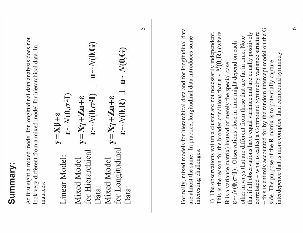
Sum
mar
y: A
t firs
t sig
ht a
mix
ed m
odel
for l
ongi
tudi
nal d
ata
anal
ysis
doe
s not
lo
ok v
ery
diff
eren
t fro
m a
mix
ed m
odel
for h
iera
rchi
cal d
ata.
In
mat
rices
: Li
near
Mod
el:
2~
(,
)N
��
�y
X�
��
0I
Mix
ed M
odel
fo
r Hie
rarc
hica
l D
ata:
2
~(
,)
~(
,)
NN
��
��
�y
X�Zu
��
0I
u0G
Mix
ed M
odel
fo
r Lon
gitu
dina
l D
ata:
~
(,
)~
(,
)N
N�
��
�y
X�Zu
��
0R
u0G
6
Form
ally
, mix
ed m
odel
s for
hie
rarc
hica
l dat
a an
d fo
r lon
gitu
dina
l dat
a ar
e al
mos
t the
sam
e. I
n pr
actic
e, lo
ngitu
dina
l dat
a in
trodu
ces s
ome
inte
rest
ing
chal
leng
es:
1) T
he o
bser
vatio
ns w
ithin
a c
lust
er a
re n
ot n
eces
saril
y in
depe
nden
t. Th
is is
the
reas
on fo
r the
bro
ader
con
ditio
ns th
at
~(
,)
N�
0R
(whe
re
R is
a v
aria
nce
mat
rix) i
nste
ad o
f mer
ely
the
spec
ial c
ase:
2
~(
,)
N�
I�
0.
Obs
erva
tions
clo
se in
tim
e m
ight
dep
end
on e
ach
othe
r in
way
s tha
t are
diff
eren
t fro
m th
ose
that
are
far i
n tim
e. N
ote
that
if a
ll ob
serv
atio
ns h
ave
equa
l var
ianc
e an
d ar
e eq
ually
pos
itive
ly
corr
elat
ed –
wha
t is c
alle
d a
Com
poun
d Sy
mm
etry
var
ianc
e st
ruct
ure
– th
is is
ent
irely
acc
ount
ed fo
r by
the
rand
om in
terc
ept m
odel
on
the
G
side
. The
pur
pose
of t
he R
mat
rix is
to p
oten
tially
cap
ture
in
terd
epen
ce th
at is
mor
e co
mpl
ex th
an c
ompo
und
sym
met
ry.

7
2) T
he m
ean
resp
onse
may
dep
end
on ti
me
in w
ays t
hat a
re fa
r mor
e co
mpl
ex th
an is
typi
cal f
or o
ther
type
s of p
redi
ctor
s. D
epen
ding
on
the
time
scal
e of
the
obse
rvat
ions
, it m
ay b
e ne
cess
ary
to u
se
poly
nom
ial m
odel
s, as
ympt
otic
mod
els,
Four
ier a
naly
sis (
orth
ogon
al
trigo
nom
etric
func
tions
) or s
plin
es th
at a
dapt
to d
iffer
ent f
eatu
res o
f th
e re
latio
nshi
p in
diff
eren
t per
iods
of t
imes
. 3)
The
re c
an b
e m
any
parti
ally
con
foun
ded
'cloc
ks' i
n th
e sa
me
anal
ysis
: per
iod-
age-
coho
rt ef
fect
s, ag
e an
d tim
e re
lativ
e to
a fo
cal
even
t suc
h as
giv
ing
birth
, inj
ury,
aro
usal
from
com
a, e
tc.
8
4) S
ome
phen
omen
a su
ch a
s per
iodi
c pa
ttern
s may
mor
e ap
prop
riate
ly
be m
odel
ed w
ith fi
xed
effe
cts (
FE) i
f the
y ar
e de
term
inis
tic (e
.g.
seas
onal
per
iodi
c va
riatio
n) o
r with
rand
om e
ffec
ts (R
E), t
he R
mat
rix
in p
artic
ular
, if t
hey
are
stoc
hast
ic (r
ando
m c
yclic
var
iatio
n su
ch a
s su
nspo
t cyc
les o
r, pe
rhap
s, ci
rcad
ian
cycl
es).
Thes
e sl
ides
focu
s on
the
sim
ple
func
tions
of t
ime
and
the
R si
de.
Lab
3 in
trodu
ces m
ore
com
plex
form
s for
func
tions
of t
ime.

9
Take
1: T
he b
asic
idea
s
10
A tr
aditi
onal
exa
mpl
e
Figu
re 1
: Pot
hoff
and
Roy
den
tal m
easu
rem
ents
in b
oys a
nd g
irls
.
Bal
ance
d da
ta:
�ev
eryo
ne m
easu
red
at
the
sam
e se
t of a
ges
�co
uld
use
a cl
assi
cal
repe
ated
mea
sure
s an
alys
is
Som
e te
rmin
olog
y:
Clu
ster
: the
set o
f ob
serv
atio
ns o
n on
e su
bjec
t O
ccas
ion:
obs
erva
tions
at
a g
iven
tim
e fo
r eac
h su
bjec
t
age
distance
202530
89
1012
14
M16
M05
89
1012
14
M02
M11
89
1012
14
M07
M08
M03
M12
M13
M14
M09
202530
M15
202530
M06
M04
M01
M10
F10
F09
F06
F01
F05
202530
F07
202530
F02
89
1012
14
F08
F03
89
1012
14
F04
F11
11
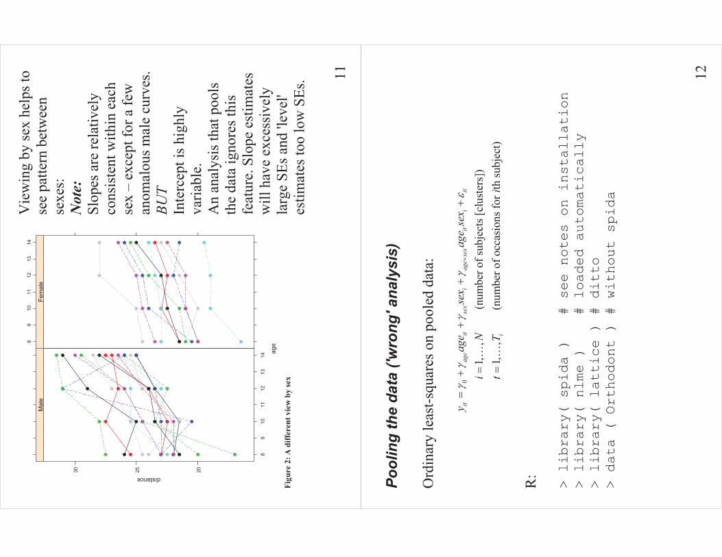
Figu
re 2
: A d
iffer
ent v
iew
by
sex
Vie
win
g by
sex
help
s to
see
patte
rn b
etw
een
sexe
s:
Not
e:Sl
opes
are
rela
tivel
y co
nsis
tent
with
in e
ach
sex
– ex
cept
for a
few
an
omal
ous m
ale
curv
es.
BUT
Inte
rcep
t is h
ighl
y va
riabl
e.
An
anal
ysis
that
poo
ls
the
data
igno
res t
his
feat
ure.
Slo
pe e
stim
ates
w
ill h
ave
exce
ssiv
ely
larg
e SE
s and
'lev
el'
estim
ates
too
low
SEs
.
age
distance
202530
89
1011
1213
14
Mal
e
89
1011
1213
14
Fem
ale
12
Pool
ing
the
data
('w
rong
' ana
lysi
s)
Ord
inar
y le
ast-s
quar
es o
n po
oled
dat
a:
0
1,,
(num
ber o
f sub
ject
s [cl
uste
rs])
1,,
(num
ber o
f occ
asio
ns fo
r th
subj
ect)
itag
eit
sex
iag
ese
xit
iit
i
yag
ese
xag
ese
xi
Nt
Ti
��
��
�
��
��
�
� �� �
R:
> library( spida ) # see notes on installation
> library( nlme ) # loaded automatically
> library( lattice ) # ditto
> data ( Orthodont ) # without spida

13
> head(Orthodont)
distance age Subject Sex
1 26.0 8 M01 Male
2 25.0 10 M01 Male
3 29.0 12 M01 Male
4 31.0 14 M01 Male
5 21.5 8 M02 Male
6 22.5 10 M02 Male
> dd <- Orthodont
> tab(dd, ~Sex)
Sex
Male Female Total
64 44 108
> dd$Sub <- reorder( dd$Subject, dd$distance)
# for plotting
14
##
OLS
Pool
ed M
odel
> fit <- lm ( distance ~ age * Sex , dd)
> summary(fit)
. . .
Coefficients:
Estimate Std. Error t value Pr(>|t|)
(Intercept) 16.3406 1.4162 11.538 < 2e-16 ***
age 0.7844 0.1262 6.217 1.07e-08 ***
SexFemale 1.0321 2.2188 0.465 0.643
age:SexFemale -0.3048 0.1977 -1.542 0.126
Residual standard error: 2.257 on 104 degrees of freedom
Multiple R-squared: 0.4227, Adjusted R-squared: 0.4061
F-statistic: 25.39 on 3 and 104 DF, p-value: 2.108e-12
Note that both SexFemale and age:SexFemale have
large p-values. Are you tempted to just drop
both of them?

15
Check the joint hypothesis that they are
BOTH 0.
> wald( fit, "Sex")
numDF denDF F.value p.value
Sex
2
104
14.9
7688
<.0
0001
Coefficients Estimate Std.Error DF t-value p-value
SexFemale 1.032102 2.218797 104 0.465163 0.64279
age:SexFemale -0.304830 0.197666 104 -1.542143 0.12608
This analysis suggests that we could drop one
or the other but not both! Which one should we
choose? To respect the principle of marginality
we should drop the interaction, not the main
effect of Sex. This leads us to:
16
> fit2 <- lm( distance ~ age + Sex ,dd )
> summary( fit2 )
Coefficients:
Estimate Std. Error t value Pr(>|t|)
(Intercept) 17.70671 1.11221 15.920 < 2e-16 ***
age 0.66019 0.09776 6.753 8.25e-10 ***
SexFemale -2.32102 0.44489 -5.217 9.20e-07 ***
and we conclude there is an effect of Sex of
jaw size but did not find evidence that the
rate of growth is different.
Revisiting the graph we saw earlier:
17
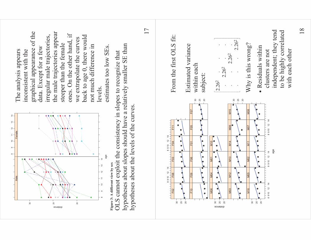
Fi
gure
3: A
diff
eren
t vie
w b
y se
x
The
anal
ysis
app
ears
in
cons
iste
nt w
ith th
e gr
aphi
cal a
ppea
ranc
e of
the
data
. Exc
ept f
or a
few
irr
egul
ar m
ale
traje
ctor
ies,
the
mal
e tra
ject
orie
s app
ear
stee
per t
han
the
fem
ale
ones
. On
the
othe
r han
d, if
w
e ex
trapo
late
the
curv
es
back
to a
ge 0
, the
re w
ould
no
t muc
h di
ffer
ence
in
leve
ls.
estim
ates
too
low
SEs
.
OLS
can
not e
xplo
it th
e co
nsis
tenc
y in
slop
es to
reco
gniz
e th
at
hypo
thes
es a
bout
slop
es sh
ould
hav
e a
rela
tivel
y sm
alle
r SE
than
hy
poth
eses
abo
ut th
e le
vels
of t
he c
urve
s.
age
distance
202530
89
1011
1213
14
Mal
e
89
1011
1213
14
Fem
ale
18
From
the
first
OLS
fit:
Estim
ated
var
ianc
e w
ithin
eac
h su
bjec
t:
22
22
2.26
..
..
2.26
..
..
2.26
..
..
2.26
�
�
�
�
�
�
�
�
��
Why
is th
is w
rong
?
�R
esid
uals
with
in
clus
ters
are
not
in
depe
nden
t; th
ey te
nd
to b
e hi
ghly
cor
rela
ted
with
eac
h ot
her
age
distance
202530
89
1012
14
M16
M05
89
1012
14
M02
M11
89
1012
14
M07
M08
M03
M12
M13
M14
M09
202530
M15
202530
M06
M04
M01
M10
F10
F09
F06
F01
F05
202530
F07
202530
F02
89
1012
14
F08
F03
89
1012
14
F04
F11

19
Fi
tted
lines
in ‘d
ata
spac
e’.
ag
e
distance 202530
89
1011
1213
14
Mal
e
89
1011
1213
14
Fem
ale
20
Det
erm
inin
g th
e in
terc
ept a
nd sl
ope
of
each
line
ag
e
distance 15202530
05
10
Mal
e
15202530
Fem
ale

21
Fitte
d lin
es in
‘d
ata’
spac
e
ag
e
distance 152025
05
10
Mal
e
Fem
ale
22
Fitte
d ‘li
nes’
in
‘bet
a’ sp
ace
��ag
e
��0 16.0
16.5
17.0
17.5
0.4
0.5
0.6
0.7
0.8
0.9
M
ale
Fe
mal
e

23
Fixe
d ef
fect
s re
gres
sion
mod
el
See
Pa
ul D
. Alli
son
(200
5) F
ixed
Effe
cts R
egre
ssio
n M
etho
ds fo
r Lo
ngitu
dina
l Dat
a U
sing
SAS
. SA
S In
stitu
te –
a g
reat
boo
k on
bas
ics
of m
ixed
mod
els!
�Tr
eat S
ubje
ct a
s a fa
ctor
�Lo
se S
ex u
nles
s it i
s con
stru
cted
as a
Sub
ject
con
trast
�Fi
ts a
sepa
rate
OLS
mod
el to
eac
h su
bjec
t:
itia
geit
iti
age
y�
��
��
��
R
: >
24
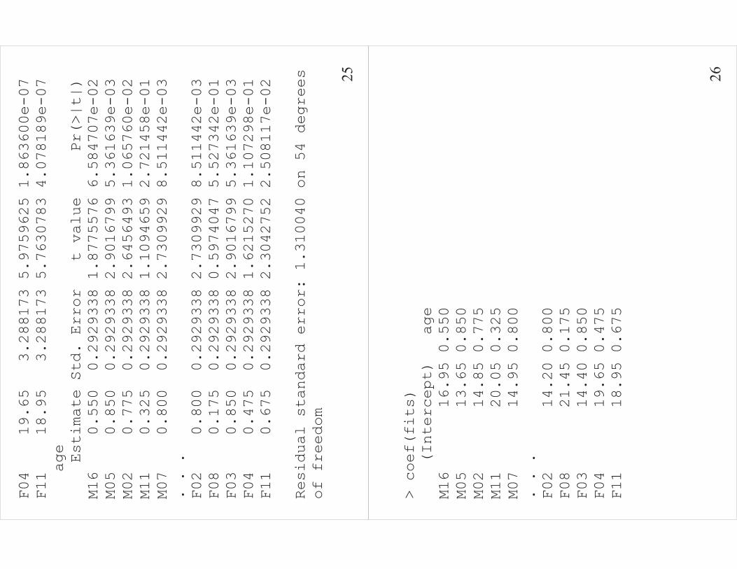
## Fixed model
> fits <- lmList(distance ~ age | Subject,dd)
> summary(fits)
Call:
Model: distance ~ age | Subject
Data: dd
Coefficients:
(Intercept)
Estimate Std. Error t value Pr(>|t|)
M16 16.95 3.288173 5.1548379 3.695247e-06
M05 13.65 3.288173 4.1512411 1.181678e-04
M02 14.85 3.288173 4.5161854 3.458934e-05
M11 20.05 3.288173 6.0976106 1.188838e-07
. . .
F02 14.20 3.288173 4.3185072 6.763806e-05
F08 21.45 3.288173 6.5233789 2.443813e-08
F03 14.40 3.288173 4.3793313 5.509579e-05
25
F04 19.65 3.288173 5.9759625 1.863600e-07
F11 18.95 3.288173 5.7630783 4.078189e-07
age
Estimate Std. Error t value Pr(>|t|)
M16 0.550 0.2929338 1.8775576 6.584707e-02
M05 0.850 0.2929338 2.9016799 5.361639e-03
M02 0.775 0.2929338 2.6456493 1.065760e-02
M11 0.325 0.2929338 1.1094659 2.721458e-01
M07 0.800 0.2929338 2.7309929 8.511442e-03
. . .
F02 0.800 0.2929338 2.7309929 8.511442e-03
F08 0.175 0.2929338 0.5974047 5.527342e-01
F03 0.850 0.2929338 2.9016799 5.361639e-03
F04 0.475 0.2929338 1.6215270 1.107298e-01
F11 0.675 0.2929338 2.3042752 2.508117e-02
Residual standard error: 1.310040 on 54 degrees
of freedom
26
> coef(fits)
(Intercept) age
M16 16.95 0.550
M05 13.65 0.850
M02 14.85 0.775
M11 20.05 0.325
M07 14.95 0.800
. . .
F02 14.20 0.800
F08 21.45 0.175
F03 14.40 0.850
F04 19.65 0.475
F11 18.95 0.675
27
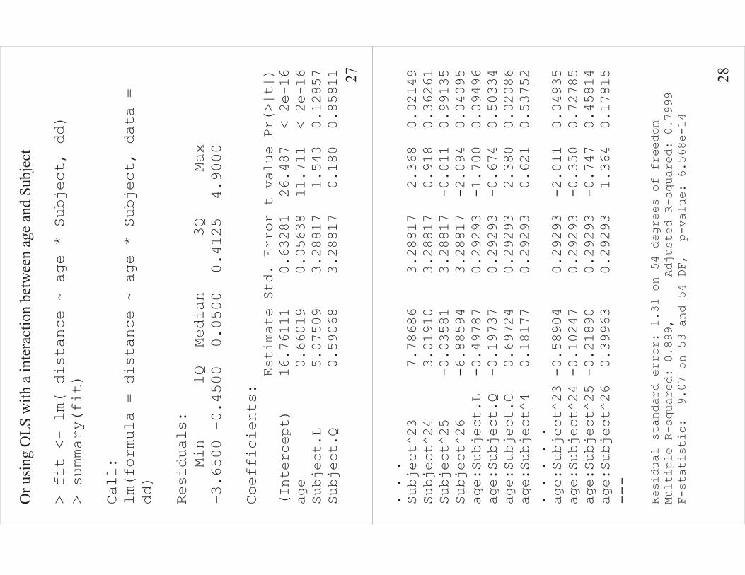
Or u
sing
OLS
with
a in
tera
ctio
n be
twee
n ag
e an
d Su
bjec
t
> fit <- lm( distance ~ age * Subject, dd)
> summary(fit)
Call:
lm(formula = distance ~ age * Subject, data =
dd)
Residuals:
Min 1Q Median 3Q Max
-3.6500 -0.4500 0.0500 0.4125 4.9000
Coefficients:
Estimate Std. Error t value Pr(>|t|)
(Intercept) 16.76111 0.63281 26.487 < 2e-16
age 0.66019 0.05638 11.711 < 2e-16
Subject.L 5.07509 3.28817 1.543 0.12857
Subject.Q 0.59068 3.28817 0.180 0.85811
28
. . .
Subject^23 7.78686 3.28817 2.368 0.02149
Subject^24 3.01910 3.28817 0.918 0.36261
Subject^25 -0.03581 3.28817 -0.011 0.99135
Subject^26 -6.88594 3.28817 -2.094 0.04095
age:Subject.L -0.49787 0.29293 -1.700 0.09496
age:Subject.Q -0.19737 0.29293 -0.674 0.50334
age:Subject.C 0.69724 0.29293 2.380 0.02086
age:Subject^4 0.18177 0.29293 0.621 0.53752
. . . . .
age:Subject^23 -0.58904 0.29293 -2.011 0.04935
age:Subject^24 -0.10247 0.29293 -0.350 0.72785
age:Subject^25 -0.21890 0.29293 -0.747 0.45814
age:Subject^26 0.39963 0.29293 1.364 0.17815
---
Residual standard error: 1.31 on 54 degrees of freedom
Multiple R-squared: 0.899, Adjusted R-squared: 0.7999
F-statistic: 9.07 on 53 and 54 DF, p-value: 6.568e-14

29
> predict( fit)
1 2 3 4 5 6 7 8 9 10
24.90 26.80 28.70 30.60 21.05 22.60 24.15 25.70 22.00 23.50
11 12 13 14 15 16 17 18 19 20
25.00 26.50 26.10 26.45 26.80 27.15 20.45 22.15 23.85 25.55
. . . .
101 102 103 104 105 106 107 108
17.15 18.05 18.95 19.85 24.35 25.70 27.05 28.40
> dd$distance.ols <- predict( fit )
> some( dd)
Grouped Data: distance ~ age | Subject
distance age Subject Sex Sub distance.ols
3 29.0 12 M01 Male M01 28.70
28 26.5 14 M07 Male M07 26.15
45 21.5 8 M12 Male M12 21.25
60 30.0 14 M15 Male M15 29.25
65 21.0 8 F01 Female F01 20.25
78 24.5 10 F04 Female F04 24.40
83 22.5 12 F05 Female F05 22.90
93 23.0 8 F08 Female F08 22.85
30
Estim
ated
var
ianc
e fo
r ea
ch su
bjec
t:
22
22
1.31
..
..
1.31
..
..
1.31
..
..
1.31
�
�
�
�
�
�
�
�
��
Prob
lem
s:
� N
o es
timat
e of
sex
effe
ct
� C
an't
gene
raliz
e to
po
pula
tion,
onl
y to
'new
' ob
serv
atio
ns fr
om sa
me
subj
ects
age
distance
202530
89
1012
14
M16
M05
89
1012
14
M02
M11
89
1012
14
M07
M08
M03
M12
M13
M14
M09
202530
M15
202530
M06
M04
M01
M10
F10
F09
F06
F01
F05
202530
F07
202530
F02
89
1012
14
F08
F03
89
1012
14
F04
F11

31
� C
an't
pred
ict f
or n
ew
subj
ect.
� C
an c
onst
ruct
sex
effe
ct b
ut C
I is f
or
diff
eren
ce b
etw
een
sexe
s in
this
sam
ple
�
No
auto
corr
elat
ion
in
time
ag
e
distance
202530
89
1012
14
M16
M05
89
1012
14
M02
M11
89
1012
14
M07
M08
M03
M12
M13
M14
M09
202530
M15
202530
M06
M04
M01
M10
F10
F09
F06
F01
F05
202530
F07
202530
F02
89
1012
14
F08
F03
89
1012
14
F04
F11
32
Fitt
ed li
nes i
n da
ta
spac
e �
Fem
ale
lines
low
er
and
less
stee
p �
Patte
rns w
ithin
Sex
es
not s
o ob
viou
s.
ag
e
distance
202530
89
1011
1213
14
Mal
e
89
1011
1213
14
Fem
ale
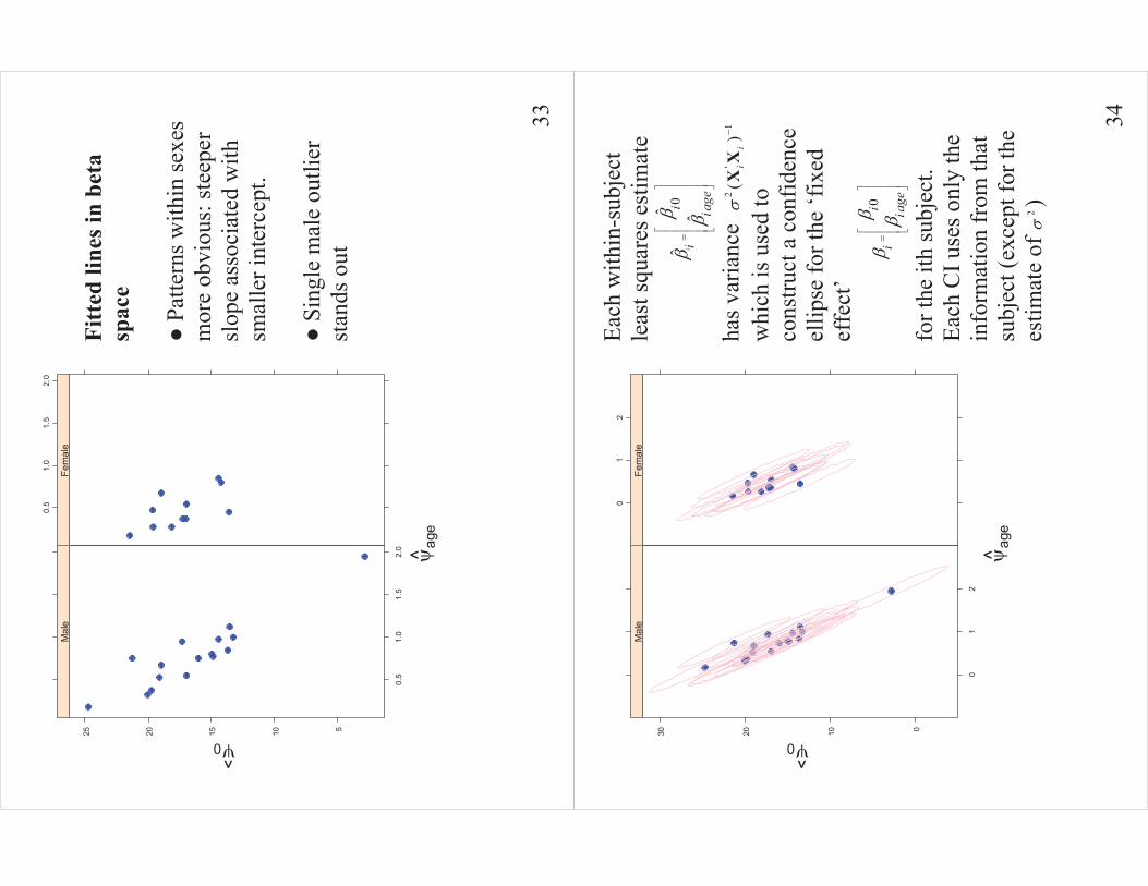
33
Fitt
ed li
nes i
n be
ta
spac
e �
Patte
rns w
ithin
sexe
s m
ore
obvi
ous:
stee
per
slop
e as
soci
ated
with
sm
alle
r int
erce
pt.
� Si
ngle
mal
e ou
tlier
st
ands
out
��ag
e
��0
510152025
0.5
1.0
1.5
2.0
Mal
e
0.5
1.0
1.5
2.0
Fem
ale
34
Each
with
in-s
ubje
ct
leas
t squ
ares
est
imat
e 0ˆ
ˆˆ
ii
iia
ge
��
��
�
�
��
�
�
�
has v
aria
nce
'
1(
)i
i�
��
XX
w
hich
is u
sed
to
cons
truct
a c
onfid
ence
el
lipse
for t
he ‘f
ixed
ef
fect
’ 0i
iia
ge
��
��
�
��
�
�
�
for t
he it
h su
bjec
t. Ea
ch C
I use
s onl
y th
e in
form
atio
n fr
om th
at
subj
ect (
exce
pt fo
r the
es
timat
e of
��)
��ag
e
��0
0102030
01
2
Mal
e
01
2
Fem
ale
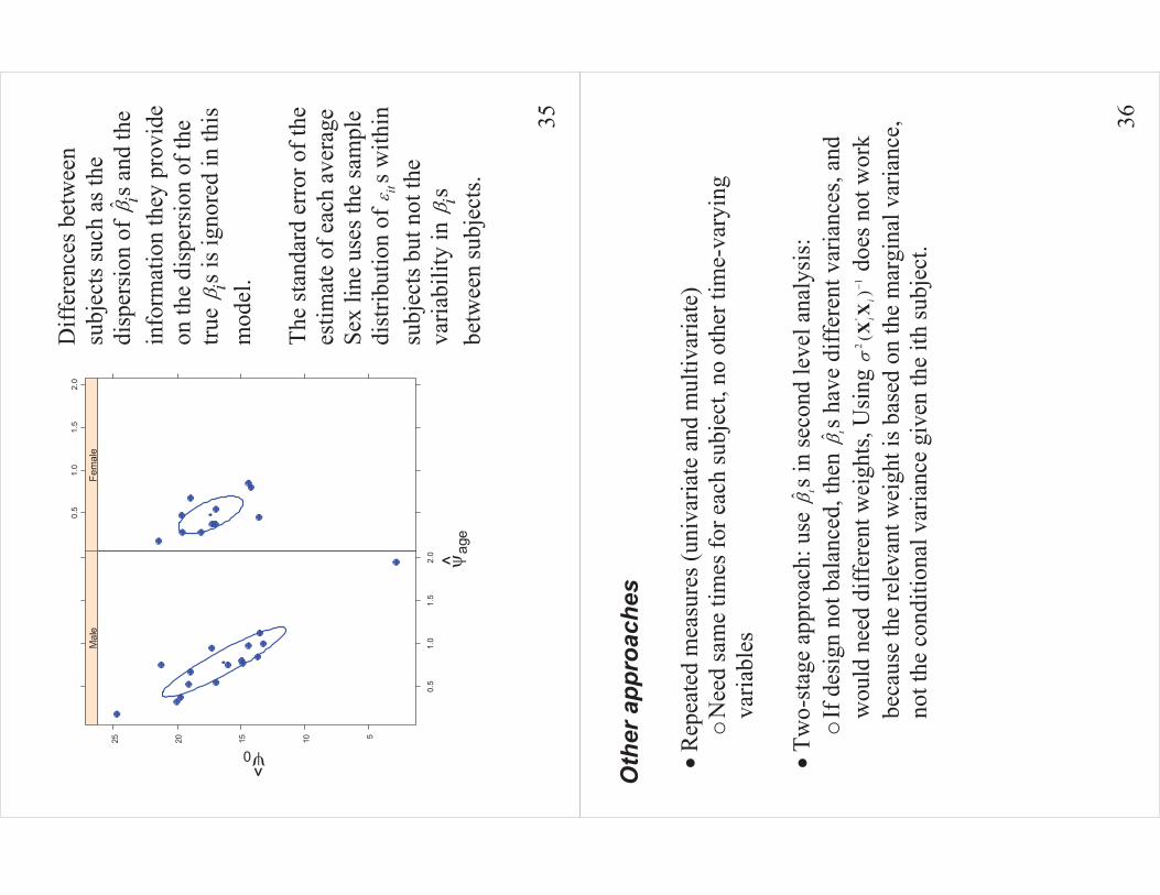
35
D
iffer
ence
s bet
wee
n su
bjec
ts su
ch a
s the
di
sper
sion
of
ˆ i�s a
nd th
e in
form
atio
n th
ey p
rovi
de
on th
e di
sper
sion
of t
he
true
i�s i
s ign
ored
in th
is
mod
el.
The
stan
dard
err
or o
f the
es
timat
e of
eac
h av
erag
e Se
x lin
e us
es th
e sa
mpl
e di
strib
utio
n of
it�s w
ithin
su
bjec
ts b
ut n
ot th
e va
riabi
lity
in
i�s
betw
een
subj
ects
.
��ag
e
��0
510152025
0.5
1.0
1.5
2.0
Mal
e
0.5
1.0
1.5
2.0
Fem
ale
36
Oth
er a
ppro
ache
s
�R
epea
ted
mea
sure
s (un
ivar
iate
and
mul
tivar
iate
) o
Nee
d sa
me
times
for e
ach
subj
ect,
no o
ther
tim
e-va
ryin
g va
riabl
es
�
Two-
stag
e ap
proa
ch: u
se
��s i
n se
cond
leve
l ana
lysi
s:
oIf
des
ign
not b
alan
ced,
then
��s h
ave
diff
eren
t var
ianc
es, a
nd
wou
ld n
eed
diff
eren
t wei
ghts
, Usi
ng
'1
()
ii
��
�X
X d
oes n
ot w
ork
beca
use
the
rele
vant
wei
ght i
s bas
ed o
n th
e m
argi
nal v
aria
nce,
no
t the
con
ditio
nal v
aria
nce
give
n th
e ith
subj
ect.
37
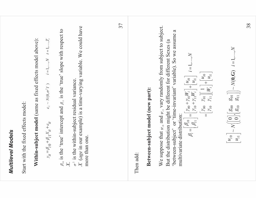
Mul
tilev
el M
odel
s St
art w
ith th
e fix
ed e
ffec
ts m
odel
:
With
in-s
ubje
ct m
odel
(sam
e as
fixe
d ef
fect
s mod
el a
bove
):
1it
itit
ii
yX
��
��
��
�
~(0
,)
iN
I�
��
�
1,
,1,
,i
iN
tT
��
��
0i� is
the
‘true
’ int
erce
pt a
nd
1i� is
the
‘true
’ slo
pe w
ith re
spec
t to
X.
�� is
the
with
in-s
ubje
ct re
sidu
al v
aria
nce.
X
(age
in o
ur e
xam
ple)
is a
tim
e-va
ryin
g va
riabl
e. W
e co
uld
have
m
ore
than
one
.
38
Then
add
:
Bet
wee
n-su
bjec
t mod
el (n
ew p
art)
:
W
e su
ppos
e th
at
0i�
and
1i
� v
ary
rand
omly
from
subj
ect t
o su
bjec
t.
But
the
dist
ribut
ion
mig
ht b
e di
ffer
ent f
or d
iffer
ent S
exes
(a
‘bet
wee
n-su
bjec
t’ o
r ‘tim
e-in
varia
nt’ v
aria
ble)
. So
we
assu
me
a m
ultiv
aria
te d
istri
butio
n:
0
11
11
11
1
1,,
1
ii
ii
ii
i
i ii
uW
iN
uW
u uW
��
��
��
�
��
��
���
��
��
����
�
��
�
�
�
�
�
�
�
�
�
��
��
��
�
�
�
�
�
�
�
�
�
��
��
��
��
��
��
��
�
0
11
1
0~
,~
(,
)1,
,0
i iug
gN
Ni
Ng
gu
����
��
��
�
�
�
��
�
�
�
��
�
�
�
��
��
��
��
�0
G�
39
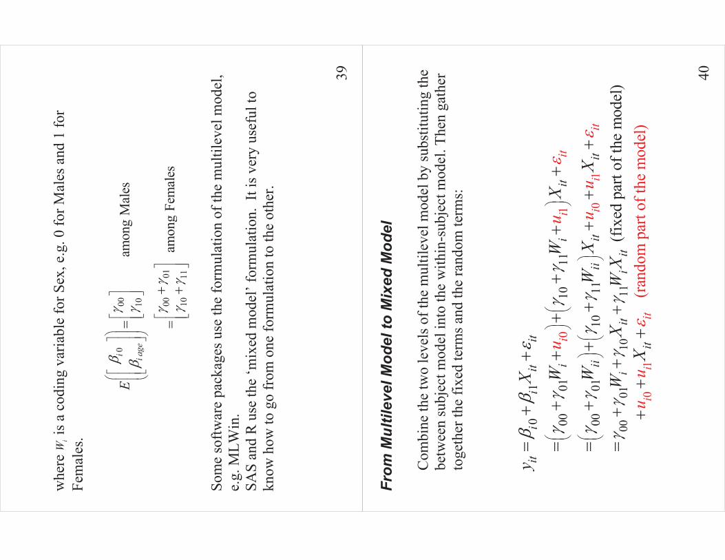
w
here
i
W is
a c
odin
g va
riabl
e fo
r Sex
, e.g
. 0 fo
r Mal
es a
nd 1
for
Fem
ales
.
0
1 11
amon
g M
ales
amon
g Fe
mal
es
i iage
E�
� ��
��
��
�� � ����
��
��
�
�
��
�
�
��
�
�
��
��
��
�
�
�
��
�
��
�
Som
e so
ftwar
e pa
ckag
es u
se th
e fo
rmul
atio
n of
the
mul
tilev
el m
odel
, e.
g. M
LWin
. SA
S an
d R
use
the
‘mix
ed m
odel
’ for
mul
atio
n. I
t is v
ery
usef
ul to
kn
ow h
ow to
go
from
one
form
ulat
ion
to th
e ot
her.
40
From
Mul
tilev
el M
odel
to M
ixed
Mod
el
C
ombi
ne th
e tw
o le
vels
of t
he m
ultil
evel
mod
el b
y su
bstit
utin
g th
e be
twee
n su
bjec
t mod
el in
to th
e w
ithin
-sub
ject
mod
el. T
hen
gath
er
toge
ther
the
fixed
term
s and
the
rand
om te
rms:
01
01
11
0
1
1
1
11
1
(fixe
d pa
rt of
the
m(ra
ndom
par
tod
el o
f t)
i
i
i
ii
itit
iti
i
ii
it
iiii
itit
iti
it
it
iti
i
it
it
WW
uu
uu
yX W
WX
WW
XX
XX
Xuu
��
��
��
�
��
��
��
��
�
�
�
��
��
��
��
��
��
��
��
��
��
��
��
����
��
� ����
��
����
��
��
��
��
��
�
��
��
��
�
��
��
�
��
�he
mod
el)

41
A
nato
my
of th
e fix
ed p
art:
1
1
(Inte
rcep
t)(b
etw
een-
sub j
ect,
time-
inva
riant
var
iabl
e)(w
ithin
-sub
ject
, tim
e-va
ryin
g va
riabl
e)(c
ross
-leve
l int
erac
tion)
i it
iitW
WX X�
� ��
��
�� �
��
��
Inte
rpre
tatio
n of
the
fixed
par
t: th
e pa
ram
eter
s ref
lect
pop
ulat
ion
aver
age
valu
es.
Ana
tom
y of
the
rand
om p
art:
For o
ne o
ccas
ion:
01
ii
iit
itt
uu
X�
��
��
Putti
ng th
e ob
serv
atio
ns o
f one
subj
ect t
oget
her:
42
0 1
1 2
11
22 3
3 4
3 44
1 1 1 1
i i
i
ii
ii
ii
ii i
i
ii
i i i
u u
u
X X X X
�
��
��
��
��
�
�
�
�
�
�
�
�
�
�
�
�
�
�
�
�
�
��
�
�
�
�
��
��
�
��
�
�
� ��
��
�
Not
e: th
e ra
ndom
-eff
ects
des
ign
uses
onl
y tim
e-va
ryin
g va
riabl
es
Dis
tribu
tion
assu
mpt
ion:
~(0
,)
inde
pend
ent o
f ~
(0,
)i
ii
uN
N�
GR
��
w
here
, so
far,
iI
��
�R

43
Not
es:
�
G (u
sual
ly) d
oes n
ot v
ary
with
i. It
is u
sual
ly a
free
pos
itive
de
finite
mat
rix o
r it m
ay b
e a
stru
ctur
ed p
os-d
ef m
atrix
. M
ore
on G
late
r. �
iR
(usu
ally
) doe
s cha
nge
with
i –
as it
mus
t if
iTis
not
co
nsta
nt.
iR
is e
xpre
ssed
as a
func
tion
of p
aram
eter
s. Th
e si
mpl
est e
xam
ple
is
ii
nn
iI
��
�
R. L
ater
we
will
use
i
R to
in
clud
e au
to-r
egre
ssiv
e pa
ram
eter
s for
long
itudi
nal
mod
elin
g.
�
We
can’
t est
imat
e G
and
Rdi
rect
ly. W
e es
timat
e th
em
thro
ugh:
'V
ar(
)i
ii
ii�
��
�V
ZG
ZR
�
44
�So
me
thin
gs c
an b
e pa
ram
etriz
ed e
ither
on
the
G-s
ide
or o
n th
e R
-sid
e. If
they
’re
done
in b
oth,
you
lose
iden
tifia
bilit
y.
Ill-c
ondi
tioni
ng d
ue “
colli
near
ity”
betw
een
the
G- a
nd R
-si
de m
odel
s is a
com
mon
pro
blem
.
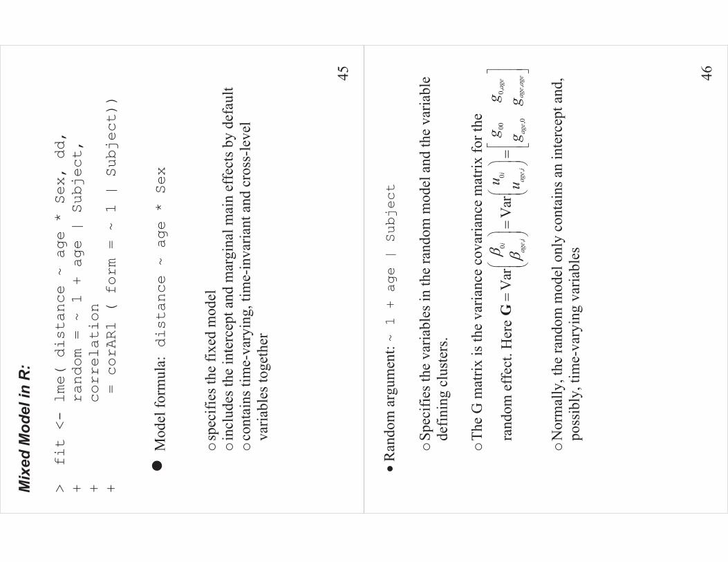
45
Mix
ed M
odel
in R
:
> fit <- lme( distance ~ age * Sex, dd,
+ random = ~ 1 + age | Subject,
+ correlation
+ = corAR1 ( form = ~ 1 | Subject))
�M
odel
form
ula: distance ~ age * Sex
osp
ecifi
es th
e fix
ed m
odel
o
incl
udes
the
inte
rcep
t and
mar
gina
l mai
n ef
fect
s by
defa
ult
oco
ntai
ns ti
me-
vary
ing,
tim
e-in
varia
nt a
nd c
ross
-leve
l va
riabl
es to
geth
er
46
�R
ando
m a
rgum
ent: ~ 1 + age | Subject
o
Spec
ifies
the
varia
bles
in th
e ra
ndom
mod
el a
nd th
e va
riabl
e de
finin
g cl
uste
rs.
o
The
G m
atrix
is th
e va
rianc
e co
varia
nce
mat
rix fo
r the
rand
om e
ffec
t. H
ere
000,
00
,,
,,0
Var
Var
age
ii
age
age
age
iag
ei
age
gg
u ug
g� �
�
��
��
�
��
��
��
��
�
��
��
��
��
�G
o
Nor
mal
ly, t
he ra
ndom
mod
el o
nly
cont
ains
an
inte
rcep
t and
, po
ssib
ly, t
ime-
vary
ing
varia
bles
47
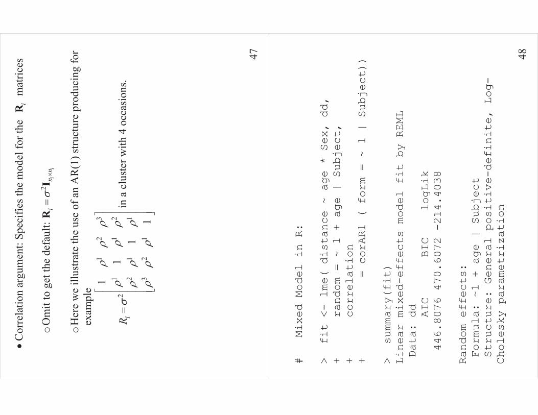
�C
orre
latio
n ar
gum
ent:
Spec
ifies
the
mod
el fo
r the
iR
mat
rices
o
Om
it to
get
the
defa
ult:
ii
nn
i�
�
�R
I
oH
ere
we
illus
trate
the
use
of a
n A
R(1
) stru
ctur
e pr
oduc
ing
for
exam
ple
12
3
11
2
21
1
32
1
11
11
iR
��
��
��
��
��
��
�
�
�
�
�
�
�
�
�
��
� in
a c
lust
er w
ith 4
occ
asio
ns.
48
# Mixed Model in R:
> fit <- lme( distance ~ age * Sex, dd,
+ random = ~ 1 + age | Subject,
+ correlation
+ = corAR1 ( form = ~ 1 | Subject))
> summary(fit)
Linear mixed-effects model fit by REML
Data: dd
AIC BIC logLik
446.8076 470.6072 -214.4038
Random effects:
Formula: ~1 + age | Subject
Structure: General positive-definite, Log-
Cholesky parametrization

49
StdDev Corr
(Intercept)
3.37
3048
2 (Intr)
00gage
0.29
0767
3 -0
.831
1101
0100
11/
gr
gg
g�
Residual 1.0919754
Correlation Structure: AR(1)
Formula: ~1 | Subject
Parameter estimate(s):
Phi
-0.4
7328
correlation between adjoining obervations
50
Fixed effects: distance ~ age * Sex
Value Std.Error DF t-value p-value
(Intercept) 16.152435 0.9984616 79 16.177323 0.0000
age 0.797950 0.0870677 79 9.164702 0.0000
SexFemale 1.264698 1.5642886 25 0.808481 0.4264
age:SexFemale -0.322243 0.1364089 79 -2.362334 0.0206
Correlation: among gammas
(Intr) age SexFml
age -0.877
SexFemale -0.638 0.559
age:SexFemale 0.559 -0.638 -0.877
Standardized Within-Group Residuals:
Min Q1 Med
Q3 Max
-3.288886631 -0.419431536 -0.001271185
0.456257976 4.203271248
Number of Observations: 108
51
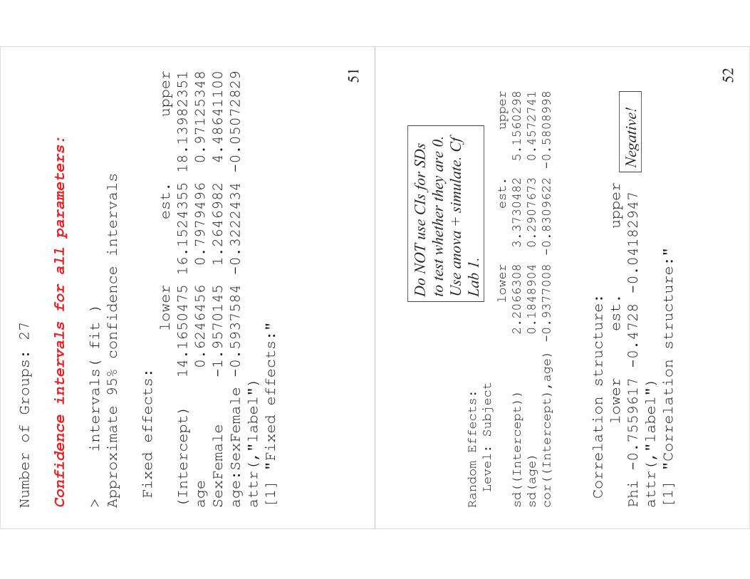
Number of Groups: 27
Confidence intervals for all parameters:
> intervals( fit )
Approximate 95% confidence intervals
Fixed effects:
lower est. upper
(Intercept) 14.1650475 16.1524355 18.13982351
age 0.6246456 0.7979496 0.97125348
SexFemale -1.9570145 1.2646982 4.48641100
age:SexFemale -0.5937584 -0.3222434 -0.05072829
attr(,"label")
[1] "Fixed effects:"
52
Random Effects:
Level: Subject
lower est. upper
sd((Intercept)) 2.2066308 3.3730482 5.1560298
sd(age) 0.1848904 0.2907673 0.4572741
cor((Intercept),age) -0.9377008 -0.8309622 -0.5808998
Correlation structure:
lower est. upper
Phi -0.7559617 -0.4728 -0.04182947
attr(,"label")
[1] "Correlation structure:"
Do
NO
T us
e C
Is fo
r SD
s to
test
whe
ther
they
are
0.
Use
ano
va +
sim
ulat
e. C
f La
b 1.
Neg
ativ
e!
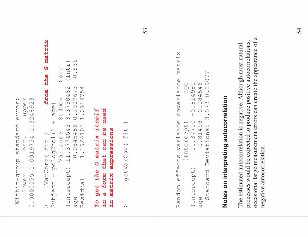
53
Within-group standard error:
lower est. upper
0.9000055 1.0919754 1.3248923
> VarCorr( fit )
from the G matrix
Subject = pdLogChol(1 + age)
Variance StdDev Corr
(Intercept) 11.3774543 3.3730482 (Intr)
age 0.0845456 0.2907673 -0.831
Residual 1.1924103 1.0919754
To get the G matrix itself
in a form that can be used
in matrix expressions
> getVarCov( fit )
54
Random effects variance covariance matrix
(Intercept) age
(Intercept) 11.37700 -0.814980
age -0.81498 0.084546
Standard Deviations: 3.373 0.29077
Not
es o
n in
terp
retin
g au
toco
rrel
atio
n Th
e es
timat
ed a
utoc
orre
latio
n is
neg
ativ
e. A
lthou
gh m
ost n
atur
al
proc
esse
s wou
ld b
e ex
pect
ed to
pro
duce
pos
itive
aut
ocor
rela
tions
, oc
casi
onal
larg
e m
easu
rem
ent e
rror
s can
cre
ate
the
appe
aran
ce o
f a
nega
tive
auto
corr
elat
ion.
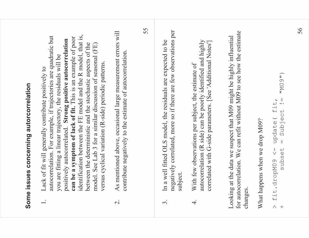
55
Som
e is
sues
con
cern
ing
auto
rcor
rela
tion
1.
Lack
of f
it w
ill g
ener
ally
con
tribu
te p
ositi
vely
to
auto
corr
elat
ion.
For
exa
mpl
e, if
traj
ecto
ries a
re q
uadr
atic
but
yo
u ar
e fit
ting
a lin
ear t
raje
ctor
y, th
e re
sidu
als w
ill b
e po
sitiv
ely
auto
corr
elat
ed.
Stro
ng p
ositi
ve a
utoc
orre
latio
n ca
n be
a sy
mpt
om o
f lac
k of
fit.
This
is a
n ex
ampl
e of
poo
r id
entif
icat
ion
betw
een
the
FE m
odel
and
the
R m
odel
, tha
t is,
betw
een
the
dete
rmin
istic
and
the
stoc
hast
ic a
spec
ts o
f the
m
odel
. See
Lab
3 fo
r a si
mila
r dis
cuss
ion
of se
ason
al (F
E)
vers
us c
yclic
al v
aria
tion
(R-s
ide)
per
iodi
c pa
ttern
s.
2.A
s men
tione
d ab
ove,
occ
asio
nal l
arge
mea
sure
men
t err
ors w
ill
cont
ribut
e ne
gativ
ely
to th
e es
timat
e of
aut
ocor
rela
tion.
56
3.In
a w
ell f
itted
OLS
mod
el, t
he re
sidu
als a
re e
xpec
ted
to b
e ne
gativ
ely
corr
elat
ed, m
ore
so if
ther
e ar
e fe
w o
bser
vatio
ns p
er
subj
ect.
4.
With
few
obs
erva
tions
per
subj
ect,
the
estim
ate
of
auto
corr
elat
ion
(R si
de) c
an b
e po
orly
iden
tifie
d an
d hi
ghly
co
rrel
ated
with
G-s
ide
para
met
ers.
[See
'Add
ition
al N
otes
'] Lo
okin
g at
the
data
we
susp
ect t
hat M
09 m
ight
be
high
ly in
fluen
tial
for a
utoc
orre
latio
n. W
e ca
n re
fit w
ithou
t M09
to se
e ho
w th
e es
timat
e ch
ange
s. W
hat h
appe
ns w
hen
we
drop
M09
?
> fit.dropM09 <- update( fit,
+ subset = Subject != "M09")

57
> summary( fit.dropM09 )
Linear mixed-effects model fit by REML
Data: dd
Subset: Subject != "M09"
AIC BIC logLik
406.3080 429.7545 -194.1540
. .
.
.
.
Correlation Structure: AR(1)
Formula: ~1 | Subject
Parameter estimate(s):
Phi
-0.1246035
still negative
. .
. .
. .
58
> intervals( fit.dropM09 )
Approximate 95% confidence intervals
. . . .
Correlation structure:
lower est. upper
Phi -0.5885311 -0.1246035 0.4010562
attr(,"label")
but not significantly
[1] "Correlation structure:"

59
Mix
ed M
odel
in M
atric
es
In th
e ith
clu
ster
:
11
1
0
1
1
0 1
11
11
22
22
33
33
44
44
11
11
11
11
ii
i
i
i
itit
iit
it
ii
ii
ii
ii
ii
ii
ii
ii
ii
ii
ii
ii
itu
u
u
W
u
Wy
XX
X
yW
XW
XX
yW
XW
XX
yW
XW
XX
yW
XW
XX
��
�� � � � �
���
���
� �� �� � �
�
�
�
�
�
�
�
�
�
�
�
�
�
�
�
�
�
�
�
�
�
�
�
�
��
��
��
�
�
�
�
��
�
��
��
��
�
��
1 2 3 4i i i i
ii
ii
i
� � � ��
�
�
�
�
�
��
�
��
�y
Xu
��
��
[Cou
ld w
e fit
this
mod
el in
clu
ster
i?]
whe
re
'
~(
,)
~(
,)
~(
,)
i
i
ii
ii
ii
ii
i
NN N
��
��
�0
Gu
�u
�0
R�
0�
G�
R
60
For t
he w
hole
sam
ple
1
11
11
0
0N
NN
NN
�
�
�
�
�
�
�
�
�
�
�
�
�
�
�
�
�
��
��
�
��
�
�
�
�
�
�
�
�
��
�
��
�u
�
u
yX
��
yX
��
�
��
��
��
��
Fina
lly m
akin
g th
e co
mpl
ex lo
ok d
ecep
tivel
y si
mpl
e:
�
��
��
u�
yX
��
X�
�

61
��
�
��
u�
yX
��
X�
�
with
1V
ar(
)
Var
()
Var
()
'
N
�
�
�
�
�
�
��
��
� ��
��
�
R0
R0
R
G � V
� u �u
� �GZ
R�
�
��
��
62
Fitti
ng th
e m
ixed
mod
el
Use
Gen
eral
ized
Lea
st S
quar
es o
n
~(
,'
)N
�y
X��G
ZR
11
1ˆ
ˆˆ
''
GLS
��
��
��
��
��
�X
VX
XV
y
We
need
ˆG
LS�
to g
et V
and
vic
e ve
rsa
so o
ne a
lgor
ithm
iter
ates
from
on
e to
the
othe
r unt
il co
nver
genc
e.
Ther
e ar
e tw
o m
ain
way
s of f
ittin
g m
ixed
mod
els w
ith n
orm
al
resp
onse
s:
63
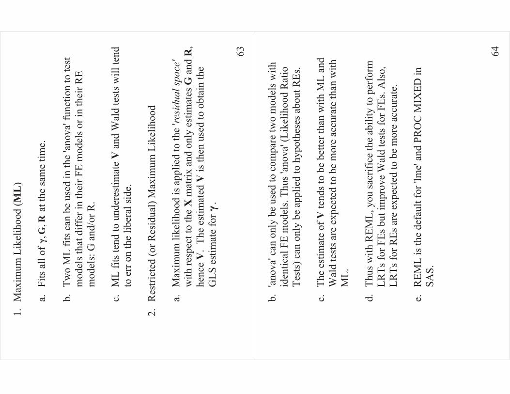
1.M
axim
um L
ikel
ihoo
d (M
L)
a.
Fits
all
of
,,
�G
R a
t the
sam
e tim
e.
b.
Two
ML
fits c
an b
e us
ed in
the
'anov
a' fu
nctio
n to
test
m
odel
s tha
t diff
er in
thei
r FE
mod
els o
r in
thei
r RE
mod
els:
G a
nd/o
r R.
c.
ML
fits t
end
to u
nder
estim
ate
V a
nd W
ald
test
s will
tend
to
err
on
the
liber
al si
de.
2.
Res
trict
ed (o
r Res
idua
l) M
axim
um L
ikel
ihoo
d
a.M
axim
um li
kelih
ood
is a
pplie
d to
the
'resi
dual
spac
e' w
ith re
spec
t to
the
X m
atrix
and
onl
y es
timat
es G
and
R,
henc
e V
. Th
e es
timat
ed V
is th
en u
sed
to o
btai
n th
e G
LS e
stim
ate
for
�.
64
b.'an
ova'
can
only
be
used
to c
ompa
re tw
o m
odel
s with
id
entic
al F
E m
odel
s. Th
us 'a
nova
' (Li
kelih
ood
Rat
io
Test
s) c
an o
nly
be a
pplie
d to
hyp
othe
ses a
bout
REs
.
c.Th
e es
timat
e of
V te
nds t
o be
bet
ter t
han
with
ML
and
Wal
d te
sts a
re e
xpec
ted
to b
e m
ore
accu
rate
than
with
M
L.
d.
Thus
with
REM
L, y
ou sa
crifi
ce th
e ab
ility
to p
erfo
rm
LRTs
for F
Es b
ut im
prov
e W
ald
test
s for
FEs
. Als
o,
LRTs
for R
Es a
re e
xpec
ted
to b
e m
ore
accu
rate
.
e.R
EML
is th
e de
faul
t for
'lm
e' an
d PR
OC
MIX
ED in
SA
S.
65
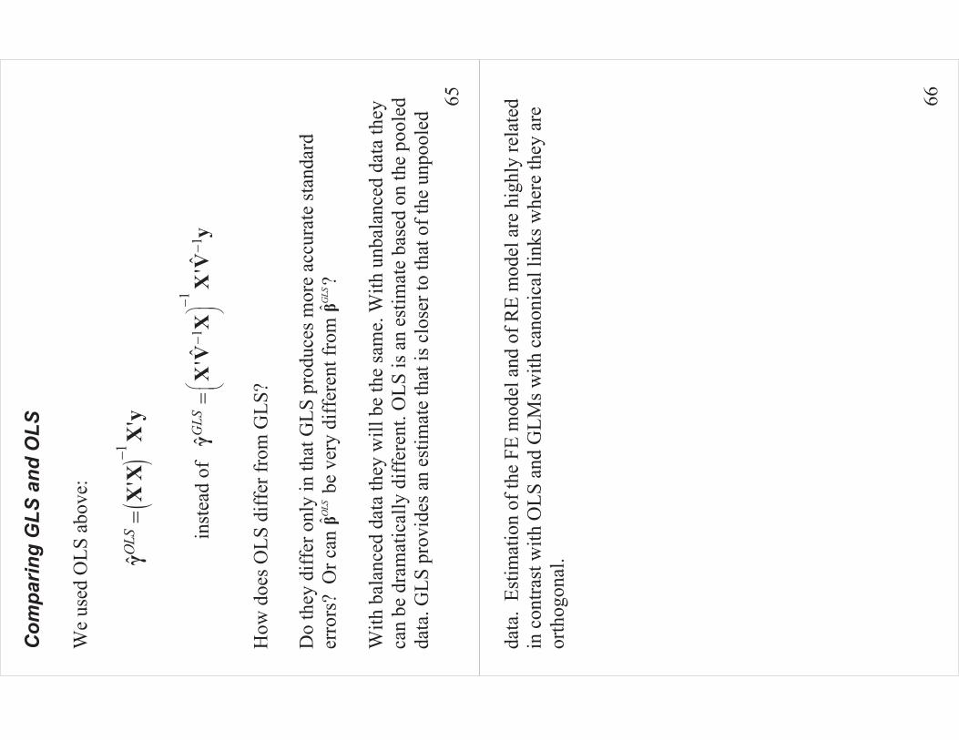
Com
parin
g G
LS a
nd O
LS
We
used
OLS
abo
ve:
!1
ˆ'
'O
LS�
��
XX
Xy
inst
ead
of
11
1ˆ
ˆˆ
''
GLS
��
��
��
��
��
�X
VX
XV
y
How
doe
s OLS
diff
er fr
om G
LS?
Do
they
diff
er o
nly
in th
at G
LS p
rodu
ces m
ore
accu
rate
stan
dard
er
rors
? O
r can
ˆO
LS�
be
very
diff
eren
t fro
m ˆ
GLS
�?
With
bal
ance
d da
ta th
ey w
ill b
e th
e sa
me.
With
unb
alan
ced
data
they
ca
n be
dra
mat
ical
ly d
iffer
ent.
OLS
is a
n es
timat
e ba
sed
on th
e po
oled
da
ta. G
LS p
rovi
des a
n es
timat
e th
at is
clo
ser t
o th
at o
f the
unp
oole
d
66
data
. Es
timat
ion
of th
e FE
mod
el a
nd o
f RE
mod
el a
re h
ighl
y re
late
d in
con
trast
with
OLS
and
GLM
s with
can
onic
al li
nks w
here
they
are
or
thog
onal
.

67
Test
ing
linea
r hyp
othe
ses
in R
H
ypot
hese
s inv
olvi
ng li
near
com
bina
tion
of th
e fix
ed e
ffec
ts
coef
ficie
nts c
an b
e te
sted
with
a W
ald
test
. The
Wal
d te
st is
ba
sed
on th
e no
rmal
app
roxi
mat
ion
for m
axim
um li
kelih
ood
estim
ator
s usi
ng th
e es
timat
ed v
aria
nce-
cova
rianc
e m
atrix
. U
sing
the
'wal
d' fu
nctio
n al
one
disp
lays
the
estim
ated
fixe
d ef
fect
s coe
ffic
ient
s and
Wal
d-ty
pe c
onfid
ence
inte
rval
s as w
ell a
s a
test
that
all
true
coef
ficie
nts a
re e
qual
0 (t
his i
s rar
ely
of a
ny
inte
rest
).
68
> wald (fit)
numDF denDF F.value p.value
4 24 952.019 <.00001
Coefficients Estimate Std.Error DF t-value p-value
(Intercept) 16.479081 1.050894 76 15.681019 <.00001
age 0.769464 0.089141 76 8.631956 <.00001
SexFemale 0.905327 1.615657 24 0.560346 0.58044
age:SexFemale -0.290920 0.137047 76 -2.122774 0.03703
Cont
inua
tion
:
Coefficients Lower 0.95 Upper 0.95
(Intercept) 14.386046 18.572117
age 0.591923 0.947004
SexFemale -2.429224 4.239878
age:SexFemale -0.563872 -0.017967
69
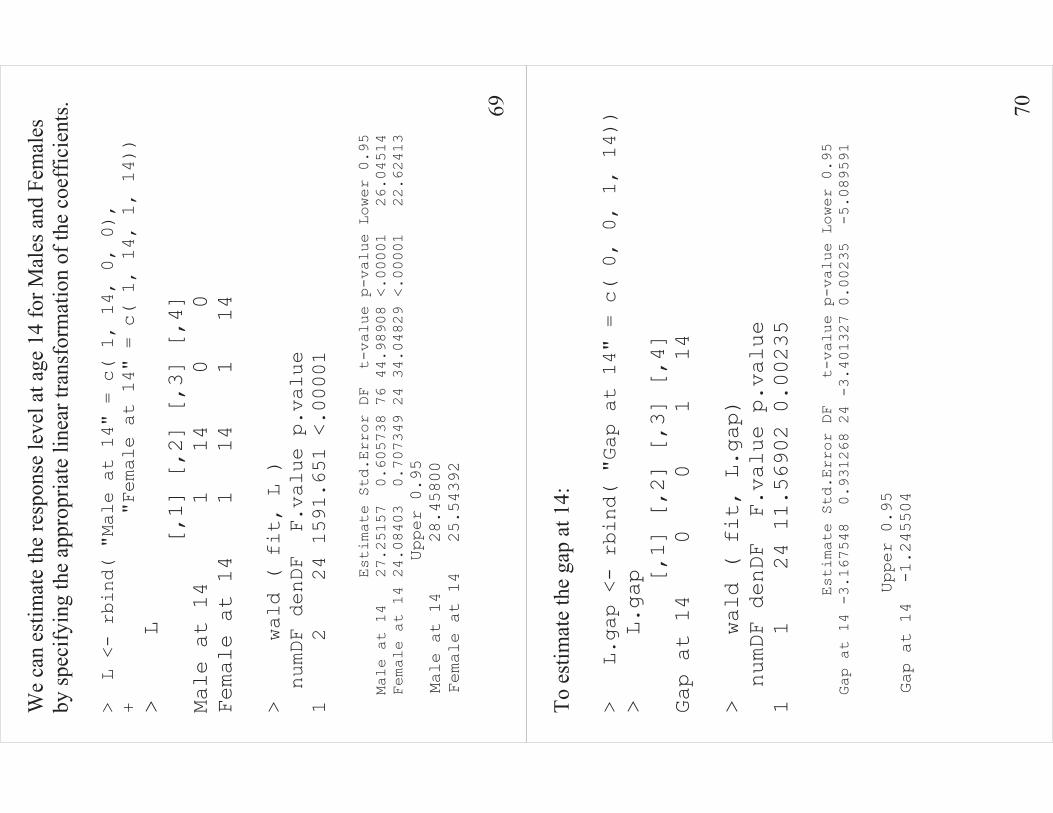
We
can
estim
ate
the
resp
onse
leve
l at a
ge 1
4 fo
r Mal
es a
nd F
emal
es
by sp
ecify
ing
the
appr
opria
te li
near
tran
sfor
mat
ion
of th
e co
effic
ient
s. > L <- rbind( "Male at 14" = c( 1, 14, 0, 0),
+ "Female at 14" = c( 1, 14, 1, 14))
> L
[,1] [,2] [,3] [,4]
Male at 14 1 14 0 0
Female at 14 1 14 1 14
> wald ( fit, L )
numDF denDF F.value p.value
1 2 24 1591.651 <.00001
Estimate Std.Error DF t-value p-value Lower 0.95
Male at 14 27.25157 0.605738 76 44.98908 <.00001 26.04514
Female at 14 24.08403 0.707349 24 34.04829 <.00001 22.62413
Upper 0.95
Male at 14 28.45800
Female at 14 25.54392
70
To e
stim
ate
the
gap
at 1
4:
> L.gap <- rbind( "Gap at 14" = c( 0, 0, 1, 14))
> L.gap
[,1] [,2] [,3] [,4]
Gap at 14 0 0 1 14
> wald ( fit, L.gap)
numDF denDF F.value p.value
1 1 24 11.56902 0.00235
Estimate Std.Error DF t-value p-value Lower 0.95
Gap at 14 -3.167548 0.931268 24 -3.401327 0.00235 -5.089591
Upper 0.95
Gap at 14 -1.245504
71
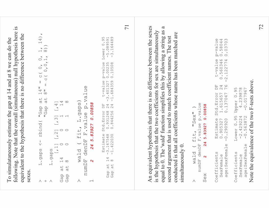
To si
mul
atan
eous
ly e
stim
ate
the
gap
at 1
4 an
d at
8 w
e ca
n do
the
follo
win
g. N
ote
that
the
over
all (
sim
ulta
neou
s) n
ull h
ypot
hesi
s her
e is
eq
uiva
lent
to th
e hy
poth
esis
that
ther
e is
no
diff
eren
ce b
etw
een
the
sexe
s.
> L.gaps <- rbind( "Gap at 14" = c( 0, 0, 1, 14),
+ "Gap at 8" = c( 0,0,1, 8))
> L.gaps
[,1] [,2] [,3] [,4]
Gap at 14 0 0 1 14
Gap at 8 0 0 1 8
> wald ( fit, L.gaps)
numDF denDF F.value p.value
12 24 5.83927
0.00858
Estimate Std.Error DF t-value p-value Lower 0.95
Gap at 14 -3.167548 0.931268 24 -3.401327 0.00235 -5.089591
Gap at 8 -1.422030 0.844256 24 -1.684359 0.10508 -3.164489
72
An
equi
vale
nt h
ypot
hesi
s tha
t the
re is
no
diff
eren
ce b
etw
een
the
sexe
s is
the
hypo
thes
is th
at th
e tw
o co
effic
ient
s for
sex
are
sim
ulta
neou
sly
equa
l to
0. T
he 'w
ald'
func
tion
sim
plifi
es th
is b
y al
low
ing
a st
ring
as a
se
cond
arg
umen
t tha
t is u
sed
to m
atch
coe
ffic
ient
nam
es. T
he te
st
cond
ucte
d is
that
all
coef
ficie
nts w
hose
nam
e ha
s bee
n m
atch
ed a
re
sim
ulta
neou
sly
0.
> wald ( fit, "Sex" )
numDF denDF F.value p.value
Sex
2 24 5.83927
0.00858
Coefficients Estimate Std.Error DF t-value p-value
SexFemale 0.905327 1.615657 24 0.560346 0.58044
age:SexFemale -0.290920 0.137047 76 -2.122774 0.03703
Coefficients Lower 0.95 Upper 0.95
SexFemale -2.429224 4.239878
age:SexFemale -0.563872 -0.017967
Not
e th
e eq
uiva
lenc
e of
the
two
F-te
sts a
bove
.
73
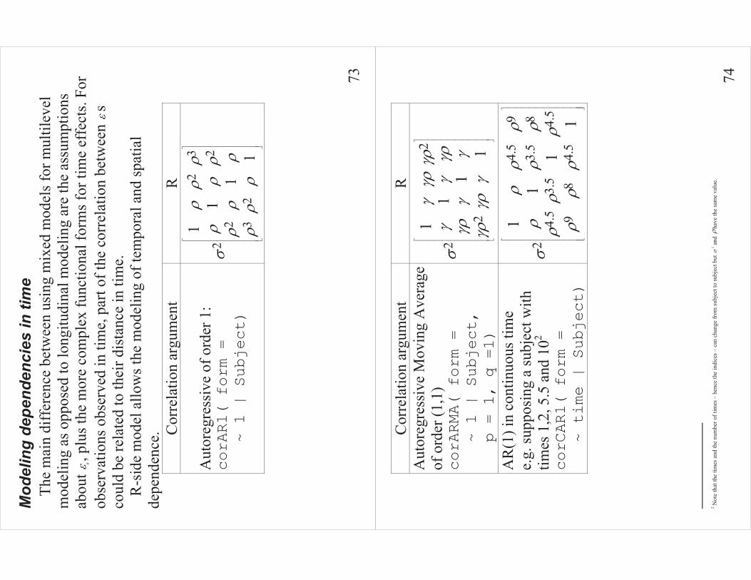
Mod
elin
g de
pend
enci
es in
tim
e Th
e m
ain
diff
eren
ce b
etw
een
usin
g m
ixed
mod
els f
or m
ultil
evel
m
odel
ing
as o
ppos
ed to
long
itudi
nal m
odel
ing
are
the
assu
mpt
ions
ab
out
it�, p
lus t
he m
ore
com
plex
func
tiona
l for
ms f
or ti
me
effe
cts.
For
obse
rvat
ions
obs
erve
d in
tim
e, p
art o
f the
cor
rela
tion
betw
een
�s
coul
d be
rela
ted
to th
eir d
ista
nce
in ti
me.
R
-sid
e m
odel
allo
ws t
he m
odel
ing
of te
mpo
ral a
nd sp
atia
l de
pend
ence
. Cor
rela
tion
argu
men
t R
Aut
oreg
ress
ive
of o
rder
1:
corAR1( form =
~ 1 | Subject)
23 2
22 3
2
11
11
��
��
��
��
��
��
�
�
�
�
�
�
�
�
�
�
�
�
��
74
Cor
rela
tion
argu
men
t R
A
utor
egre
ssiv
e M
ovin
g A
vera
ge
of o
rder
(1,1
) corARMA( form =
~ 1 | Subject,
p = 1, q =1)
2
2
211
11
���
���
���
���
��
����
�
�
�
�
�
�
�
�
�
�
�
�
��
AR
(1) i
n co
ntin
uous
tim
e e.
g. su
ppos
ing
a su
bjec
t with
tim
es 1
,2, 5
.5 a
nd 1
02 corCAR1( form =
~ time | Subject)
4.5
93.
58
24.
53.
54.
59
84.
5
11
11
��
��
��
��
��
��
�
�
�
�
�
�
�
�
�
�
�
�
�
��
2 Not
e th
at th
e tim
es a
nd th
e nu
mbe
r of t
imes
– h
ence
the
indi
ces –
can
cha
nge
from
subj
ect t
o su
bjec
t but
2
�an
d �
have
the
sam
e va
lue.

75
G-s
ide
vs. R
-sid
e
�A
few
thin
gs c
an b
e do
ne w
ith e
ither
side
. But
don
’t do
it w
ith
both
in th
e sa
me
mod
el. T
he re
dund
ant p
aram
eter
s will
not
be
iden
tifia
ble.
For
exa
mpl
e, th
e G
-sid
e ra
ndom
inte
rcep
t mod
el is
‘a
lmos
t’ eq
uiva
lent
to th
e R
-sid
e co
mpo
und
sym
met
ry m
odel
.
�W
ith O
LS th
e lin
ear p
aram
eter
s are
orth
ogon
al to
the
varia
nce
para
met
er. C
ollin
earit
y am
ong
the
linea
r par
amet
ers i
s det
erm
ined
by
the
desi
gn, X
, and
doe
s not
dep
end
on v
alue
s of p
aram
eter
s.
Com
puta
tiona
l pro
blem
s due
to c
ollin
earit
y ca
n be
add
ress
ed b
y or
thog
onal
izin
g th
e X
mat
rix.
�
With
mix
ed m
odel
s the
var
ianc
e pa
ram
eter
s are
gen
eral
ly n
ot
orth
ogon
al to
eac
h ot
her a
nd, w
ith u
nbal
ance
d da
ta, t
he li
near
pa
ram
eter
s are
not
orth
ogon
al to
the
varia
nce
para
met
ers.
76
�G
-sid
e pa
ram
eter
s can
be
high
ly c
ollin
ear e
ven
if th
e X
mat
rix is
or
thog
onal
. Cen
terin
g th
e va
riabl
es o
f the
RE
mod
el a
roun
d th
e “p
oint
of m
inim
al v
aria
nce”
will
hel
p bu
t the
resu
lting
des
ign
mat
rix m
ay b
e hi
ghly
col
linea
r.
�G
-sid
e an
d R
-sid
e pa
ram
eter
s can
be
high
ly c
ollin
ear.
The
degr
ee
of c
ollin
earit
y m
ay d
epen
d on
the
valu
e of
the
para
met
ers.
�Fo
r exa
mpl
e, o
ur m
odel
iden
tifie
s �
thro
ugh:
2
3 22
0001
210
113
2
11
31
11
11
11
ˆ1
13
11
31
13
1
gg
gg
��
��
��
��
��
��
�
�
�
�
�
�
�
� �
�
� �
�
�
� �
�
�
� �
�
�
� �
�
�
��
��
�
�
�
�
��
�
��
� ��
��
�V
For v
alue
s of
� ab
ove
0.5,
the
Hes
ssia
n is
ver
y ill
-con
ditio
ned.
The
le
sson
may
be
that
to u
se A
R, A
RM
A m
odel
s eff
ectiv
ely,
you
nee
d at
leas
t som
e su
bjec
ts o
bser
ved
on m
any
occa
sion
s.
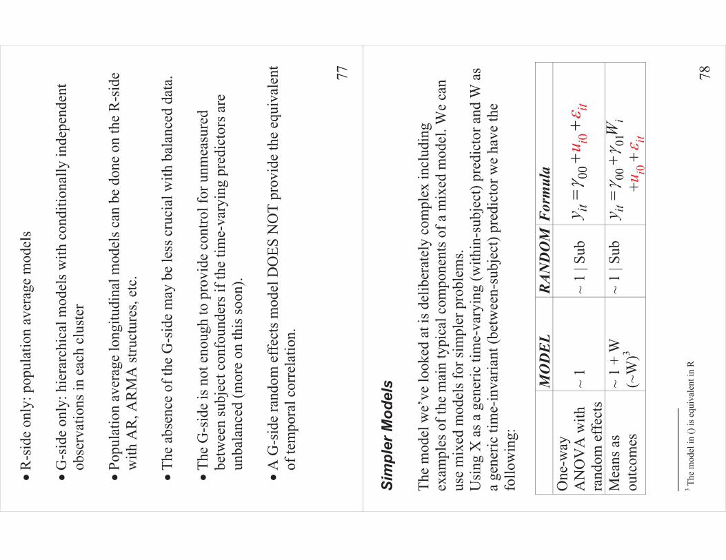
77
�R
-sid
e on
ly: p
opul
atio
n av
erag
e m
odel
s �
G-s
ide
only
: hie
rarc
hica
l mod
els w
ith c
ondi
tiona
lly in
depe
nden
t ob
serv
atio
ns in
eac
h cl
uste
r
�Po
pula
tion
aver
age
long
itudi
nal m
odel
s can
be
done
on
the
R-s
ide
with
AR
, AR
MA
stru
ctur
es, e
tc.
�
The
abse
nce
of th
e G
-sid
e m
ay b
e le
ss c
ruci
al w
ith b
alan
ced
data
.
�Th
e G
-sid
e is
not
eno
ugh
to p
rovi
de c
ontro
l for
unm
easu
red
betw
een
subj
ect c
onfo
unde
rs if
the
time-
vary
ing
pred
icto
rs a
re
unba
lanc
ed (m
ore
on th
is so
on).
�
A G
-sid
e ra
ndom
eff
ects
mod
el D
OES
NO
T pr
ovid
e th
e eq
uiva
lent
of
tem
pora
l cor
rela
tion.
78
Sim
pler
Mod
els
The
mod
el w
e’ve
look
ed a
t is d
elib
erat
ely
com
plex
incl
udin
g ex
ampl
es o
f the
mai
n ty
pica
l com
pone
nts o
f a m
ixed
mod
el. W
e ca
n us
e m
ixed
mod
els f
or si
mpl
er p
robl
ems.
Usi
ng X
as a
gen
eric
tim
e-va
ryin
g (w
ithin
-sub
ject
) pre
dict
or a
nd W
as
a ge
neric
tim
e-in
varia
nt (b
etw
een-
subj
ect)
pred
icto
r we
have
the
follo
win
g:
M
OD
EL
RAN
DO
M F
orm
ula
One
-way
A
NO
VA
with
ra
ndom
eff
ects
~
1 ~
1 | S
ub
0iit
itu
y�
���
��
�
Mea
ns a
s ou
tcom
es
~ 1
+ W
(~
W)3
~ 1
| Sub
0
i
ii
it
tu
Wy
��
���
���
��
�
3 The
mod
el in
() is
equ
ival
ent i
n R

79
One
-way
A
NC
OV
A w
ith
rand
om e
ffec
ts
~ 1
+ X
(~X
) ~
1 | S
ub
0
1
iit
itit
uy
X�
� ���
���
� �
Ran
dom
co
effic
ient
s m
odel
~
1 +
X (~
X)
~ 1+
X|S
ub
1
01
ii
itit it
itu
uy
X X�
��
���
��
��
�
Inte
rcep
ts a
nd
slop
es a
s ou
tcom
es
~ 1
+ X
+
W +
X:W
(~
X*W
)
~ 1+
X|S
ub
1
1 01
i
ii
itit
iit
itit
W
uu
Wy
XX
X
��
��
�
����
�
��� �
�
�� �
Non
- ran
dom
sl
opes
~
1 +
X
+ W
+ X
:W
(~ X
*W)
~ 1
| Sub
0
1
1
i
i
itit
iit itW
Wy
XX
�
��
��
� ��
���
��� ��
�
�
80
BLU
PS: E
stim
atin
g W
ithin
-Sub
ject
Effe
cts
We’
ve se
en h
ow to
est
imat
e �
, G a
nd R
. Now
we
cons
ider
0 1i
ii�
��
��
�
�
��
.
We’
ve a
lread
y es
timat
ed
i� u
sing
the
fixed
-eff
ects
mod
el w
ith a
OLS
re
gres
sion
with
in e
ach
subj
ect.
Cal
l thi
s est
imat
or:
i�. H
ow g
ood
is
it?
1'
ˆV
ar(
)i
ii
i�
��
��
��
��
��
��
XX
Can
we
do b
ette
r? W
e ha
ve a
noth
er ‘e
stim
ator
’ of
i�.
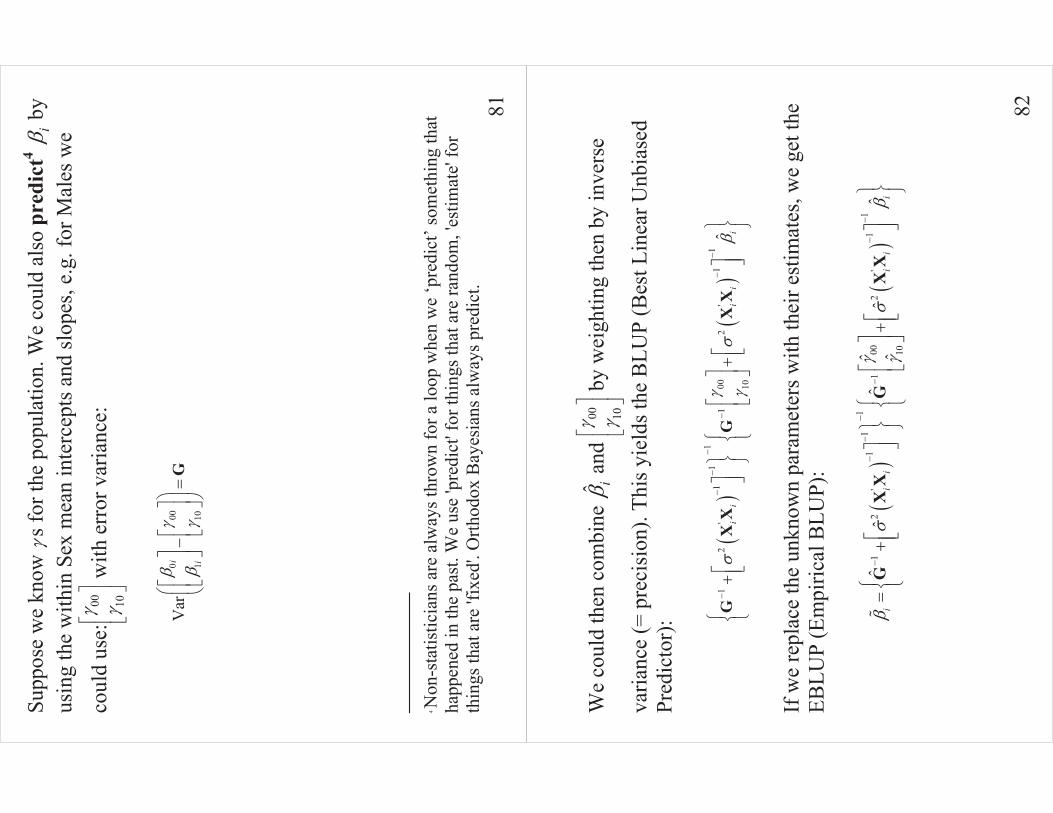
81
Supp
ose
we
know
�s f
or th
e po
pula
tion.
We
coul
d al
so p
redi
ct4
i� b
y us
ing
the
with
in S
ex m
ean
inte
rcep
ts a
nd sl
opes
, e.g
. for
Mal
es w
e co
uld
use:
1� ��� �
�
�
�� w
ith e
rror
var
ianc
e:
0
00
110
Var
i i
��
��
��
�
�
��
��
�
�
��
��
��
G
4 Non
-sta
tistic
ians
are
alw
ays t
hrow
n fo
r a lo
op w
hen
we
‘pre
dict
’ som
ethi
ng th
at
happ
ened
in th
e pa
st. W
e us
e 'p
redi
ct' f
or th
ings
that
are
rand
om, '
estim
ate'
for
thin
gs th
at a
re 'f
ixed
'. O
rthod
ox B
ayes
ians
alw
ays p
redi
ct.
82
We
coul
d th
en c
ombi
ne
i� a
nd
1� ��� �
�
�
�� b
y w
eigh
ting
then
by
inve
rse
varia
nce
(= p
reci
sion
). Th
is y
ield
s the
BLU
P (B
est L
inea
r Unb
iase
d Pr
edic
tor)
:
!
!
11
11
11
'1
'
1
ˆi
ii
ii
��
��
�
��
��
���
��
��
�
"#
�
"#
�
�
��
$%
$%
�
�
�
��
��
&'
��
&'
GX
XG
XX
If w
e re
plac
e th
e un
know
n pa
ram
eter
s with
thei
r est
imat
es, w
e ge
t the
EB
LUP
(Em
piric
al B
LUP)
:
!
!
11
11
11
'1
'
1ˆˆ
ˆˆ
ˆˆ
ˆi
ii
ii
i
��
��
��
��
��
���
��
��
�
"#
�
"#
�
�
��
�$
%$
%�
�
�
�
��
�&
'�
�&
'G
XX
GX
X�

83
The
EBLU
P ‘o
ptim
ally
’ com
bine
s the
info
rmat
ion
from
the
ith c
lust
er
with
the
info
rmat
ion
from
the
othe
r clu
ster
s. W
e bo
rrow
stre
ngth
fr
om th
e ot
her c
lust
ers.
The
proc
ess ‘
shrin
ks’
i� to
war
ds
1ˆ ˆ� ��� �
�
�
�� a
long
a p
ath
dete
rmin
ed b
y th
e
locu
s of o
scul
atio
n of
the
fam
ilies
of e
llips
es w
ith sh
ape
Gar
ound
1ˆ ˆ� ��� �
�
�
��
and
shap
e
!1'
ˆi
i�
��
�
�
��
XX
aro
und
i�.
84
� Th
e sl
ope
of th
e B
LUP
is c
lose
to th
e po
pula
tion
slop
e bu
t th
e le
vel o
f the
BLU
P is
cl
ose
to th
e le
vel o
f the
B
LUE
This
sugg
ests
that
G h
as
a la
rge
varia
nce
for
inte
rcep
ts a
nd a
smal
l va
rianc
e fo
r slo
pes
age
distance
202530
89
1012
14
M16
M05
89
1012
14
M02
M11
89
1012
14
M07
M08
M03
M12
M13
M14
M09
202530
M15
202530
M06
M04
M01
M10
F10
F09
F06
F01
F05
202530
F07
202530
F02
89
1012
14
F08
F03
89
1012
14
F04
F11
Pop
nB
LUE
BLU
P
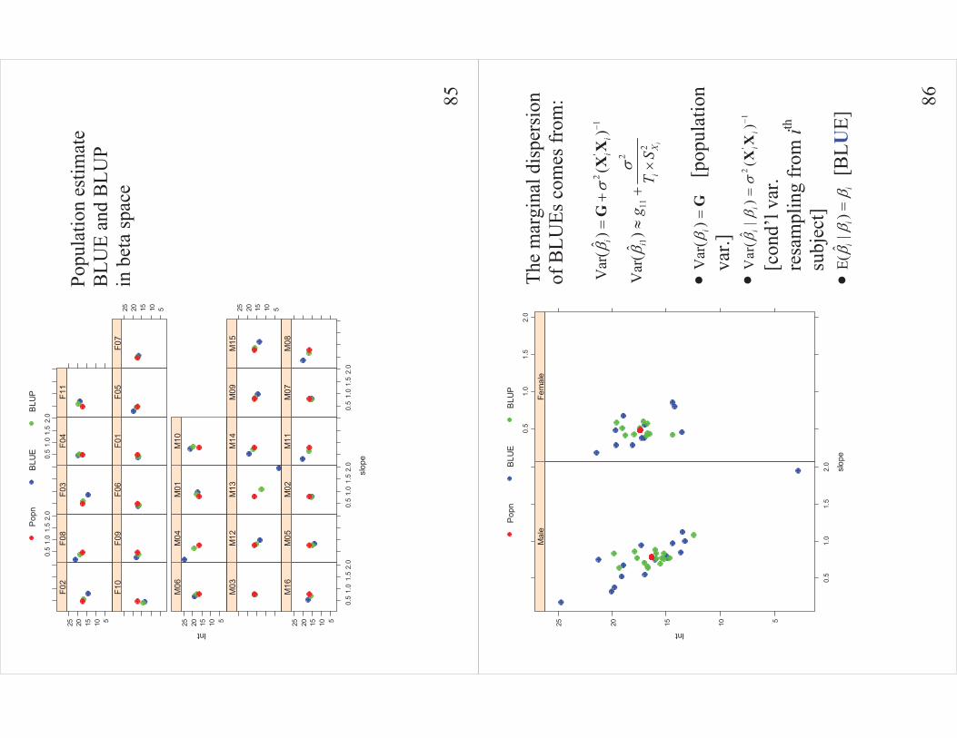
85
Popu
latio
n es
timat
e B
LUE
and
BLU
P in
bet
a sp
ace
slop
e
Int
510152025
0.5
1.0
1.5
2.0
M16
M05
0.5
1.0
1.5
2.0
M02
M11
0.5
1.0
1.5
2.0
M07
M08
M03
M12
M13
M14
M09
510152025M
15510152025
M06
M04
M01
M10
F10
F09
F06
F01
F05
510152025F0
7510152025
F02
0.5
1.0
1.5
2.0
F08
F03
0.5
1.0
1.5
2.0
F04
F11
Pop
nB
LUE
BLU
P
86
The
mar
gina
l dis
pers
ion
of B
LUEs
com
es fr
om:
2
'1
2
111
2
ˆV
ar(
)(
)
ˆV
ar(
)i
ii
i
ii
X
gT
S
��
��
��
�
(�
GX
X
�V
ar(
) i��
G
[pop
ulat
ion
var.]
�
2'
1ˆ
Var
(|
)(
)i
ii
i�
��
��
XX
[c
ond’
l var
. re
sam
plin
g fr
om ith
su
bjec
t] �
ˆE(
|)
ii
i�
��
� [
BLU
E]
slop
e
Int
510152025
0.5
1.0
1.5
2.0
Mal
e
0.5
1.0
1.5
2.0
Fem
ale
Pop
nB
LUE
BLU
P
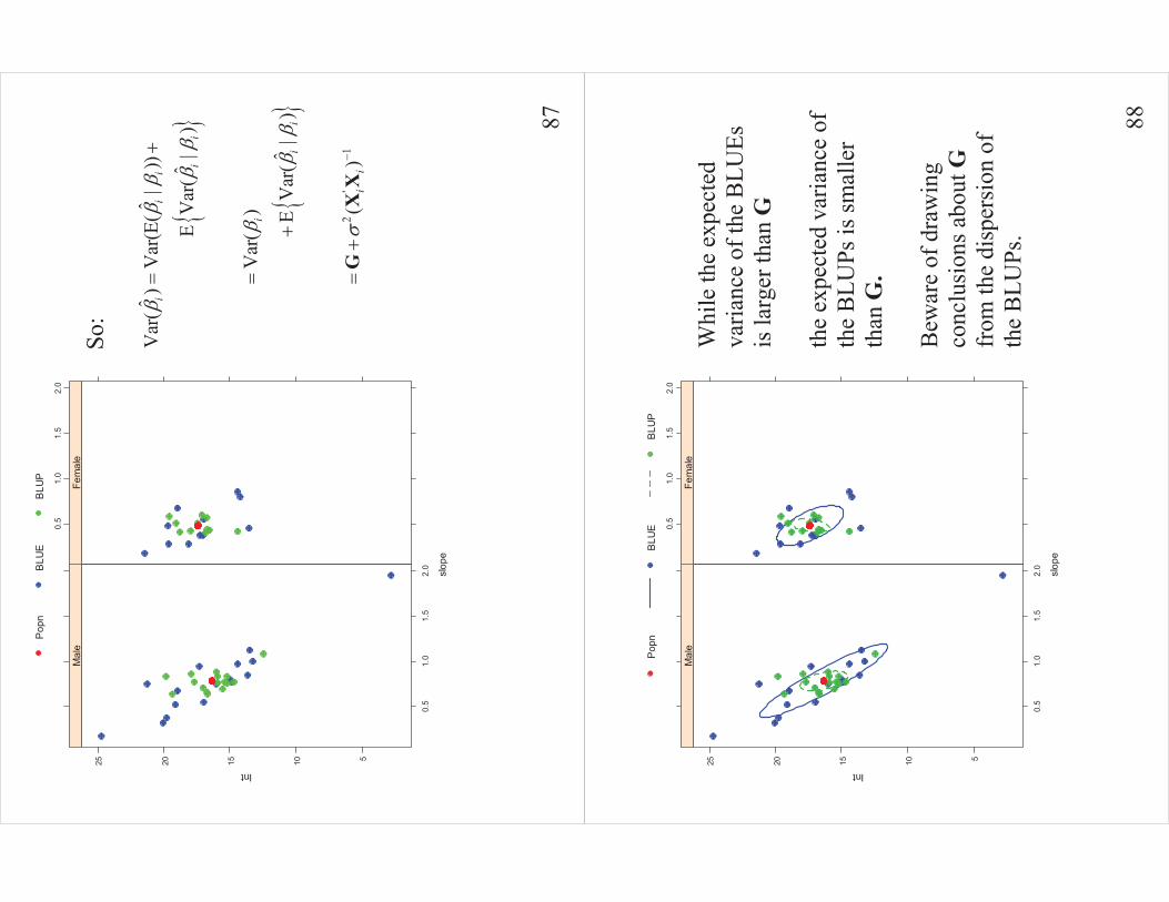
87
So:
)*
)*
2'
1
ˆˆ
Var
()
Var
(E(
|)) ˆ
EV
ar(
|)
Var
()
ˆE
Var
(|
)
()
ii
i ii
i
ii
ii
��
� ��
�
��
��
��
�
�
��
GX
X
slop
e
Int
510152025
0.5
1.0
1.5
2.0
Mal
e
0.5
1.0
1.5
2.0
Fem
ale
Pop
nB
LUE
BLU
P
88
W
hile
the
expe
cted
va
rianc
e of
the
BLU
Es
is la
rger
than
G
the
expe
cted
var
ianc
e of
th
e B
LUPs
is sm
alle
r th
an G
. B
ewar
e of
dra
win
g co
nclu
sion
s abo
ut G
fr
om th
e di
sper
sion
of
the
BLU
Ps.
sl
ope
Int
510152025
0.5
1.0
1.5
2.0
Mal
e
0.5
1.0
1.5
2.0
Fem
ale
Pop
nB
LUE
BLU
P

89
The
estim
ate
of G
can
be
uns
tabl
e an
d of
ten
colla
pses
to si
ngul
arity
le
adin
g to
non
-co
nver
genc
e fo
r man
y m
etho
ds.
Poss
ible
rem
edie
s:
- Rec
entre
X n
ear p
oint
of
min
imal
var
ianc
e,
- Use
a sm
alle
r G
- Cha
nge
the
mod
el
sl
ope
Int
510152025
0.5
1.0
1.5
2.0
Mal
e
0.5
1.0
1.5
2.0
Fem
ale
Pop
nB
LUE
BLU
P
90
Whe
re th
e EB
LUP
com
es fr
om :
look
ing
at a
sin
gle
subj
ect
N
ote
that
the
EBLU
P’s
slop
e is
clo
se to
the
slop
e of
the
popu
latio
n es
timat
e (i.
e. th
e m
ale
popu
latio
n co
nditi
onin
g on
bet
wee
n-su
bjec
t pre
dict
ors)
whi
le
the
leve
l of t
he li
ne is
cl
ose
to le
vel o
f the
B
LUE.
Th
e re
lativ
e pr
ecis
ions
of
the
BLU
E an
d of
the
popu
latio
n es
timat
e on
sl
ope
and
leve
l ar
e re
flect
ed th
roug
h th
e sh
apes
of G
and
2
'1
()
ii
��
XX
M11 ag
e
distance
222324252627
89
1011
1213
14
Pop
nB
LUE
BLU
P
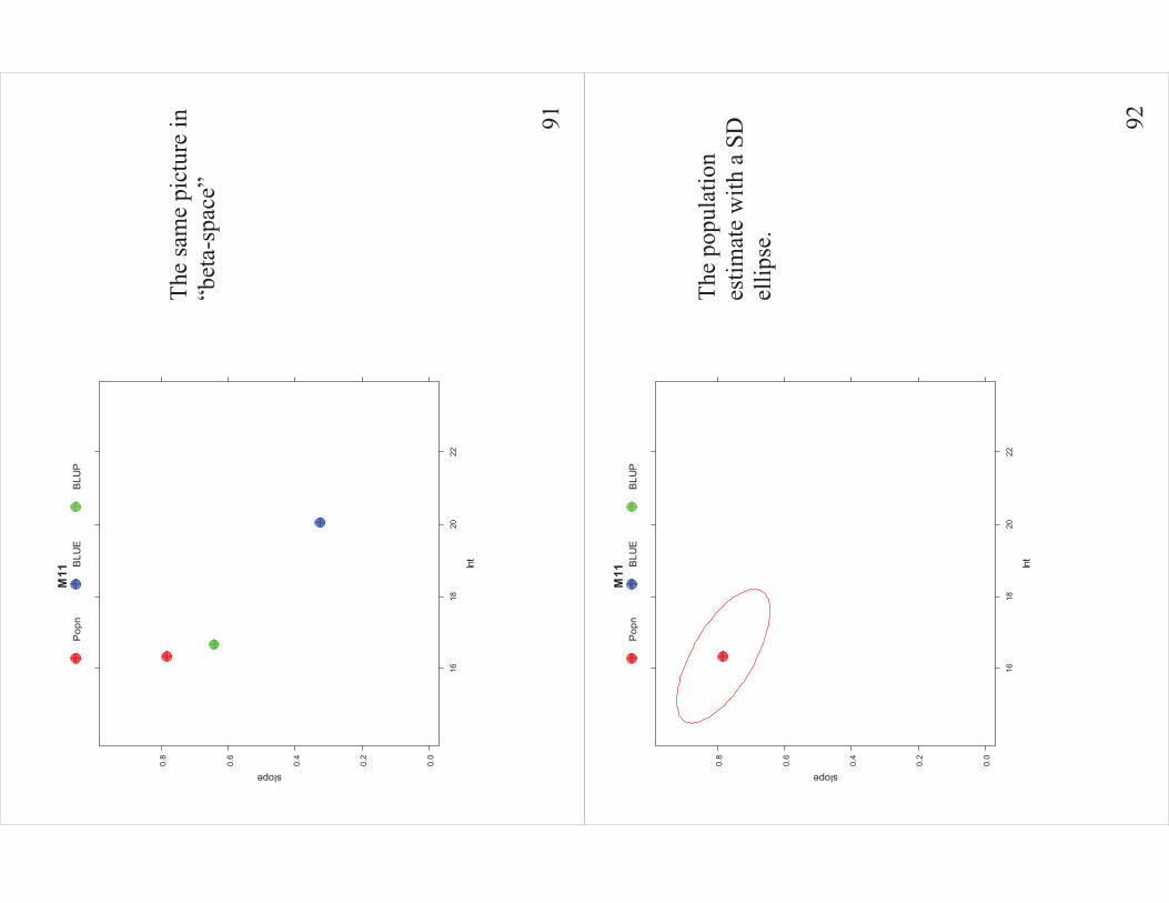
91
Th
e sa
me
pict
ure
in
“bet
a-sp
ace”
M11
Int
slope
0.0
0.2
0.4
0.6
0.8
1618
2022
Pop
nB
LUE
BLU
P
92
The
popu
latio
n es
timat
e w
ith a
SD
el
lipse
.
M11
Int
slope
0.0
0.2
0.4
0.6
0.8
1618
2022
Pop
nB
LUE
BLU
P
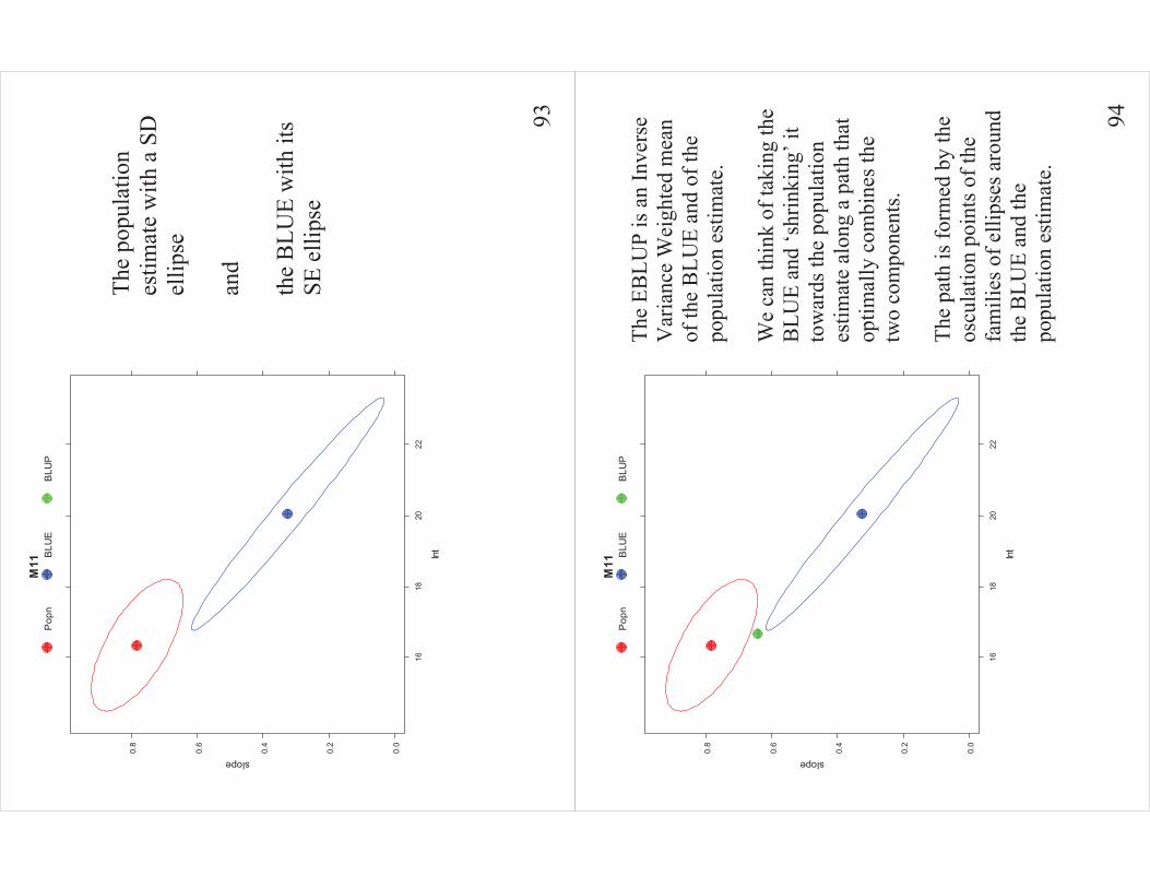
93
The
popu
latio
n es
timat
e w
ith a
SD
el
lipse
an
d
the
BLU
E w
ith it
s SE
elli
pse
M11
Int
slope
0.0
0.2
0.4
0.6
0.8
1618
2022
Pop
nB
LUE
BLU
P
94
The
EBLU
P is
an
Inve
rse
Var
ianc
e W
eigh
ted
mea
n of
the
BLU
E an
d of
the
popu
latio
n es
timat
e.
We
can
thin
k of
taki
ng th
e B
LUE
and
‘shr
inki
ng’ i
t to
war
ds th
e po
pula
tion
estim
ate
alon
g a
path
that
op
timal
ly c
ombi
nes t
he
two
com
pone
nts.
The
path
is fo
rmed
by
the
oscu
latio
n po
ints
of t
he
fam
ilies
of e
llips
es a
roun
d th
e B
LUE
and
the
popu
latio
n es
timat
e.
M11
Int
slope
0.0
0.2
0.4
0.6
0.8
1618
2022
Pop
nB
LUE
BLU
P
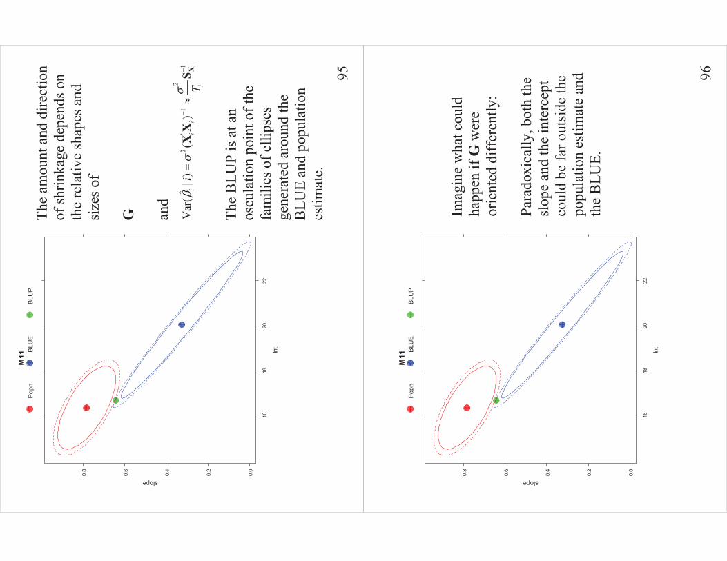
95
The
amou
nt a
nd d
irect
ion
of sh
rinka
ge d
epen
ds o
n th
e re
lativ
e sh
apes
and
si
zes o
f G
an
d 2
2'
11
ˆV
ar(
|)
()
ii
ii
i
iT�
��
��
�(
XX
XS
The
BLU
P is
at a
n os
cula
tion
poin
t of t
he
fam
ilies
of e
llips
es
gene
rate
d ar
ound
the
BLU
E an
d po
pula
tion
estim
ate.
M11
Int
slope
0.0
0.2
0.4
0.6
0.8
1618
2022
Pop
nB
LUE
BLU
P
96
Im
agin
e w
hat c
ould
ha
ppen
if G
wer
e or
ient
ed d
iffer
ently
: Pa
rado
xica
lly, b
oth
the
slop
e an
d th
e in
terc
ept
coul
d be
far o
utsi
de th
e po
pula
tion
estim
ate
and
the
BLU
E.
M11
Int
slope
0.0
0.2
0.4
0.6
0.8
1618
2022
Pop
nB
LUE
BLU
P
97
Whe
n is
a B
LU
P a
BL
UPP
ER
? Th
e ra
tiona
le b
ehin
d B
LUPs
is b
ased
on
exch
ange
abili
ty. N
o ou
tsid
e in
form
atio
n sh
ould
mak
e th
is c
lust
er st
and
out f
rom
the
othe
rs a
nd th
e m
ean
of th
e po
pula
tion
dese
rves
the
sam
e w
eigh
t in
pred
ictio
n fo
r thi
s cl
uste
r as i
t des
erve
s for
any
oth
er c
lust
er th
at d
oesn
’t st
and
out.
If a
clu
ster
stan
ds o
ut so
meh
ow, t
hen
the
BLU
P m
ight
be
a B
LUPP
ER.
98
Inte
rpre
ting
G
The
para
met
ers o
f G g
ive
the
varia
nce
of th
e in
terc
epts
, the
var
ianc
e of
the
slop
es a
nd th
e co
varia
nce
betw
een
inte
rcep
ts a
nd th
e sl
opes
. W
ould
it m
ake
sens
e to
ass
ume
that
the
cova
rianc
e is
0 to
redu
ce th
e nu
mbe
r of p
aram
eter
s in
the
mod
el?
To a
ddre
ss th
is, c
onsi
der t
hat t
he
varia
nce
of th
e he
ight
s of i
ndiv
idua
l reg
ress
ion
lines
a fi
xed
valu
e of
X
is:
11
0001
1011
200
0111
Var
()
Var
1
11
2
XX g
gX
gg
Xg
gX
gX
��
���
��
��
�
��
�
��
� �
�
��
� �
��
��
��
�
�
� � �
�
� � �
�
��
�
�� � �
��

99
Sum
mar
izin
g:
2
100
0111
Var
()
2X
gg
Xg
X�
��
���
��
�
is q
uadr
atic
func
tion
of X
.
So
1V
ar(
)X
��
��
��
has
a m
inim
um a
t 01 11g g
�
and
the
min
imum
var
ianc
e is
2 01
0011g
gg
�
10
0
Thus
, ass
umin
g th
at th
e co
varia
nce
is 0
is e
quiv
alen
t to
assu
min
g th
at th
e m
inim
um v
aria
nce
occu
rs w
hen
X=
0. T
his i
s an
ass
umpt
ion
that
is n
ot in
varia
nt w
ith lo
catio
n tra
nsfo
rmat
ions
of
X. I
t is s
imila
r to
rem
ovin
g a
mai
n ef
fect
that
is m
argi
nal t
o an
in
tera
ctio
n in
a m
odel
, som
ethi
ng th
at sh
ould
not
be
done
with
out a
th
orou
gh u
nder
stan
ding
of i
ts c
onse
quen
ces.
Ex
ampl
e: L
et
20 1� �� �
�
�
��
�
� �
��
� a
nd
10.5
11
0.1
�
��
�
��
�G
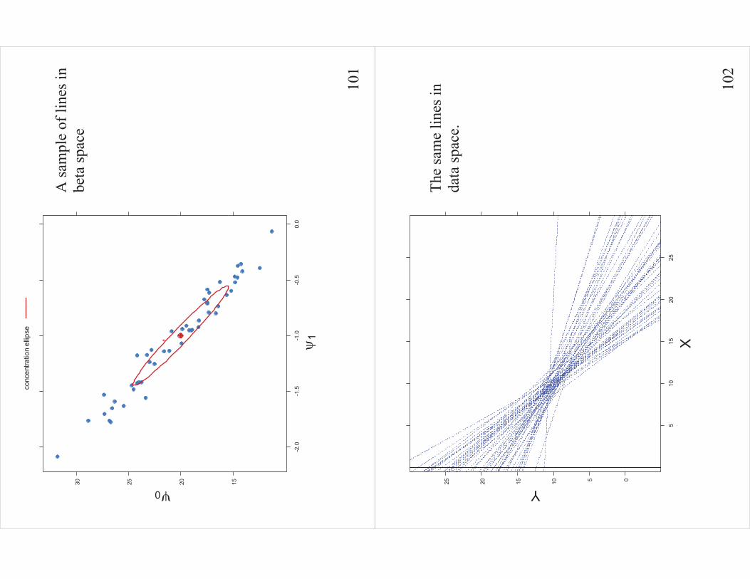
10
1
A sa
mpl
e of
line
s in
beta
spac
e
��1
��0 15202530
-2.0
-1.5
-1.0
-0.5
0.0
conc
entra
tion
ellip
se
10
2
The
sam
e lin
es in
da
ta sp
ace.
X
Y 0510152025
510
1520
25
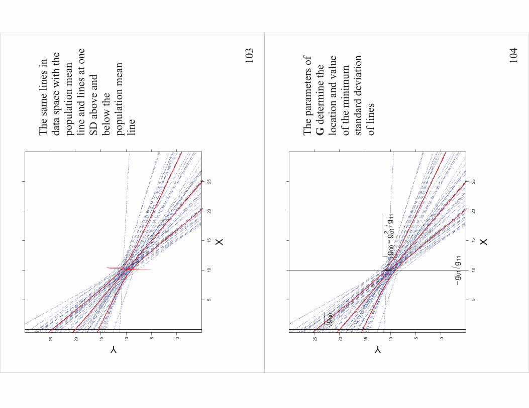
10
3
The
sam
e lin
es in
da
ta sp
ace
with
the
popu
latio
n m
ean
line
and
lines
at o
ne
SD a
bove
and
be
low
the
popu
latio
n m
ean
line
X
Y 0510152025
510
1520
25
10
4
The
para
met
ers o
f G
det
erm
ine
the
loca
tion
and
valu
e of
the
min
imum
st
anda
rd d
evia
tion
of li
nes
X
Y 0510152025
510
1520
25
��g 0
1g 1
1
�g 0
0
�g 0
0�
g 012
g 11

10
5
With
two
time-
vary
ing
varia
bles
with
rand
om e
ffec
ts, t
he G
mat
rix
wou
ld lo
ok li
ke:
000
0102
110
1112
220
2122
Var
i i i
gg
gg
gg
gg
g
� � �
��
�
�
��
�
�
��
�
�
��
�
�
��
�
�
��
��
��
���
Th
e po
int o
f min
imum
var
ianc
e is
loca
ted
at:
1
1011
12
2122
20gg
gg
gg
�
�
��
�
�
�
�
��
��
10
6
Diff
eren
ces
betw
een
lm (O
LS) a
nd lm
e (m
ixed
mod
el) w
ith
bala
nced
dat
a Ju
st lo
okin
g at
regr
essi
on c
oeff
icie
nts:
> fit.ols <- lm( distance ~ age * Sex, dd)
> fit.mm <- lme( distance ~ age * Sex, dd,
+ random = ~ 1 + age | Subject)
> summary(fit.ols)
Call:
lm(formula = distance ~ age * Sex, data = dd)
Residuals:
Min 1Q Median 3Q Max
-5.6156 -1.3219 -0.1682 1.3299 5.2469
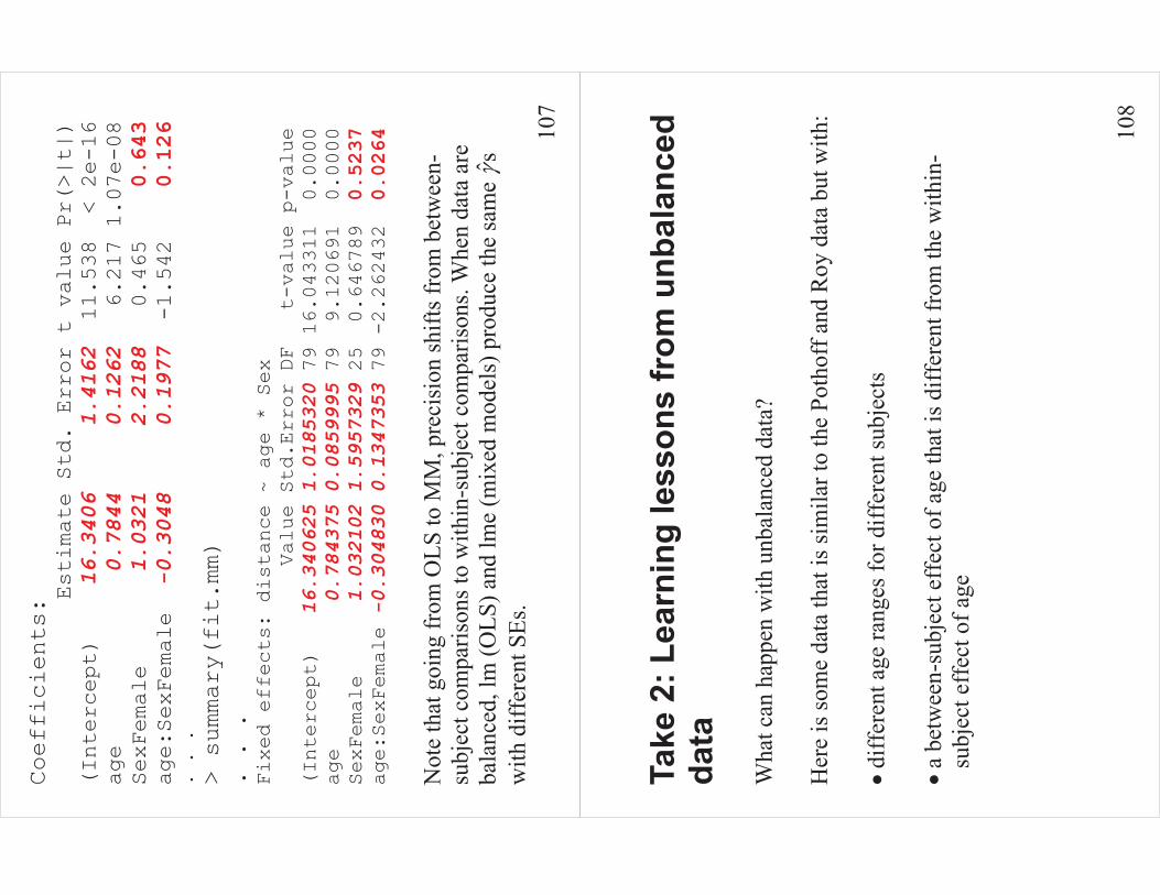
10
7
Coefficients:
Estimate Std. Error t value Pr(>|t|)
(Intercept)
16.3406 1.4162 11.538 < 2e-16
age
0.7844 0.1262 6.217 1.07e-08
SexFemale
1.0321 2.2188 0.465
0.643
age:SexFemale
-0.3048 0.1977 -1.542
0.126
. . .
> summary(fit.mm)
. . .
Fixed effects: distance ~ age * Sex
Value Std.Error DF t-value p-value
(Intercept)
16.340625 1.0185320 79 16.043311 0.0000
age
0.784375 0.0859995 79 9.120691 0.0000
SexFemale
1.032102 1.5957329 25 0.646789
0.5237
age:SexFemale-0.304830 0.1347353 79 -2.262432
0.0264
Not
e th
at g
oing
from
OLS
to M
M, p
reci
sion
shift
s fro
m b
etw
een-
subj
ect c
ompa
rison
s to
with
in-s
ubje
ct c
ompa
rison
s. W
hen
data
are
ba
lanc
ed, l
m (O
LS) a
nd lm
e (m
ixed
mod
els)
pro
duce
the
sam
e � s
w
ith d
iffer
ent S
Es.
10
8
Take
2: L
earn
ing
less
ons
from
unb
alan
ced
data
Wha
t can
hap
pen
with
unb
alan
ced
data
?
Her
e is
som
e da
ta th
at is
sim
ilar t
o th
e Po
thof
f and
Roy
dat
a bu
t with
: �
diff
eren
t age
rang
es fo
r diff
eren
t sub
ject
s �
a be
twee
n-su
bjec
t eff
ect o
f age
that
is d
iffer
ent f
rom
the
with
in-
subj
ect e
ffec
t of a
ge
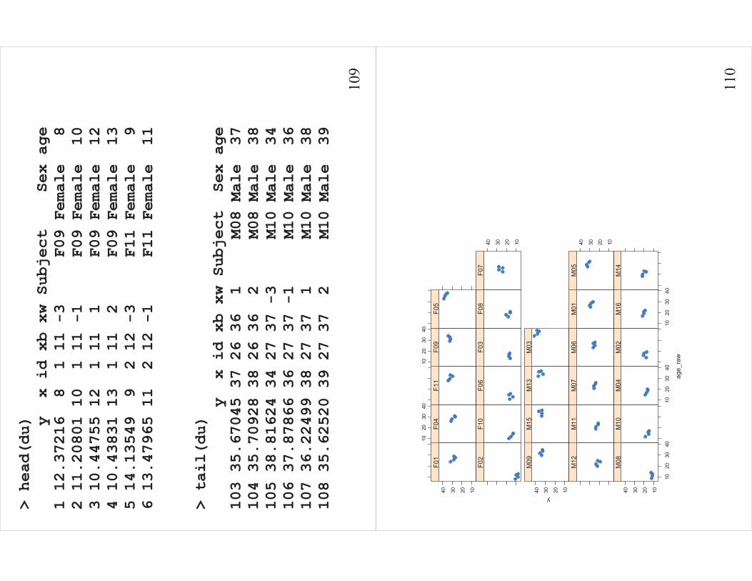
10
9
> he
ad(d
u)
y
x id
xb
xw S
ubje
ct
Se
x ag
e 1
12.3
7216
8
1 1
1 -3
F09
Fem
ale
8
2 11
.208
01 1
0 1
11
-1
F
09 F
emal
e 1
0 3
10.4
4755
12
1 1
1 1
F09
Fem
ale
12
4 10
.438
31 1
3 1
11
2
F
09 F
emal
e 1
3 5
14.1
3549
9
2 1
2 -3
F11
Fem
ale
9
6 13
.479
65 1
1 2
12
-1
F
11 F
emal
e 1
1
> ta
il(d
u)
y
x
id x
b xw
Sub
ject
Se
x ag
e 10
3 35
.670
45 3
7 26
36
1
M
08 M
ale
37
104
35.7
0928
38
26 3
6 2
M08
Mal
e 3
8 10
5 38
.816
24 3
4 27
37
-3
M
10 M
ale
34
106
37.8
7866
36
27 3
7 -1
M10
Mal
e 3
6 10
7 36
.224
99 3
8 27
37
1
M
10 M
ale
38
108
35.6
2520
39
27 3
7 2
M10
Mal
e 3
9
11
0
ag
e_ra
w
y
10203040
1020
3040
M08
M10
1020
3040
M04
M02
1020
3040
M16
M14
M12
M11
M07
M06
M01
10203040M
0510203040
M09
M15
M13
M03
F02
F10
F06
F03
F08
10203040F0
710203040
F01
1020
3040
F04
F11
1020
3040
F09
F05
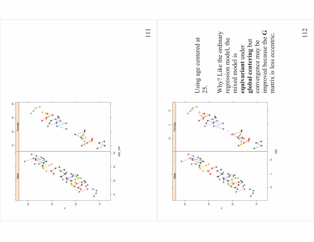
11
1
age_
raw
y
10203040
1020
3040
Mal
e
1020
3040
Fem
ale
11
2
Usi
ng a
ge c
ente
red
at
25.
Why
? Li
ke th
e or
dina
ry
regr
essi
on m
odel
, the
m
ixed
mod
el is
eq
uiva
rian
t und
er
glob
al c
ente
ring
but
co
nver
genc
e m
ay b
e im
prov
ed b
ecau
se th
e G
m
atrix
is le
ss e
ccen
tric.
age
y
10203040
-10
010
Mal
e
-10
010
Fem
ale

11
3
R c
ode
and
outp
ut
> fit <- lme( y ~ age * Sex, du,
+ random = ~ 1 + age| Subject)
> summary( fit )
Linear mixed-effects model fit by REML
Data: du
AIC BIC logLik
374.6932 395.8484 -179.3466
Random effects:
Formula: ~1 + age | Subject
Structure: General positive-definite, Log-
Cholesky parametrization
StdDev Corr
(Intercept) 9.32672995 (Intr)
age 0.05221248 0.941
Residual 0.50627022
11
4
Fixed effects: y ~ age * Sex
Value Std.Error DF t-value p-value
(Intercept) 40.26568 2.497546 79 16.122095 0.0000
age -0.48066 0.035307 79 -13.613685 0.0000
SexFemale -14.01875 3.830956 25 -3.659333 0.0012
age:SexFemale 0.05239 0.055373 79 0.946092 0.3470
Correlation:
(Intr) age SexFml
age -0.007
SexFemale -0.652 0.005
age:SexFemale 0.005 -0.638 0.058
Standardized Within-Group Residuals:
Min Q1 Med Q3 Max
-2.10716969 -0.54148659 -0.02688422 0.59030024 2.14279806
Number of Observations: 108
Number of Groups: 27
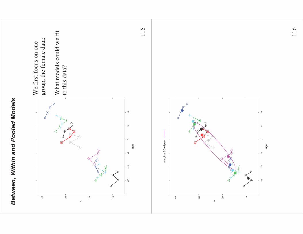
11
5
Bet
wee
n, W
ithin
and
Poo
led
Mod
els
W
e fir
st fo
cus o
n on
e gr
oup,
the
fem
ale
data
: W
hat m
odel
s cou
ld w
e fit
to
this
dat
a?
age
y
10203040
-15
-10
-50
510
11
6
age
y
10203040
-15
-10
-50
510
mar
gina
l SD
ellip
se

11
7
Reg
ress
ing
with
the
po
oled
dat
a –
igno
ring
Subj
ect –
yie
lds t
he
mar
gina
l (un
cond
ition
al)
estim
ate
of th
e sl
ope:
P�
ag
e
y
10203040
-15
-10
-50
510
mar
gina
l reg
ress
ion
line
11
8
We
coul
d re
plac
e ea
ch
Subj
ect b
y its
mea
ns fo
r x
and
y an
d us
e th
e re
sulti
ng
aggr
egat
ed d
ata
with
one
po
int f
or e
ach
Subj
ect.
ag
e
y
10203040
-15
-10
-50
510

11
9
ag
e
y
10203040
-15
-10
-50
510
disp
ersi
on e
llipse
of s
ubje
ct m
eans
12
0
Perf
orm
ing
a re
gres
sion
on
the
aggr
egat
ed d
ata
yiel
ds th
e ‘b
etw
een-
subj
ect’
regr
essi
on, i
n so
me
cont
exts
cal
led
an
‘eco
logi
cal r
egre
ssio
n’
estim
atin
g, in
som
e co
ntex
ts, t
he
'com
posi
tiona
l eff
ect'
of
age.
ag
e
y
10203040
-15
-10
-50
510
regr
essi
on o
n su
bjec
t mea
ns =
eco
logi
cal r
egre
ssio
n

12
1
We
can
com
bine
all
with
in-s
ubje
ct re
gres
sion
s to
get
a c
ombi
ned
estim
ate
of th
e w
ithin
-sub
ject
sl
ope.
Thi
s is t
he e
stim
ate
obta
ined
with
a fi
xed-
effe
cts m
odel
usi
ng a
ge
and
Subj
ect a
dditi
vely
. Eq
uiva
lent
ly, w
e ca
n pe
rfor
m a
regr
essi
on u
sing
(th
e w
ithin
-sub
ject
re
sidu
als o
f y m
inus
mea
n y)
on
(age
min
us m
ean
age)
. Q
: Whi
ch is
bet
ter:
� +,
W�or
P�?
.
age
y
10203040
-15
-10
-50
510
with
in-s
ubje
ct re
gres
sion
12
2
A: N
one.
The
y an
swer
di
ffer
ent q
uest
ions
. Ty
pica
lly,
P� w
ould
be
used
for p
redi
ctio
n ac
ross
th
e po
pula
tion;
W� fo
r ‘c
ausa
l’ in
fere
nce
cont
rolli
ng fo
r bet
wee
n-su
bjec
t con
foun
ders
, as
sum
ing
that
all
conf
ound
ers a
ffec
t all
obse
rvat
ions
sim
ilarly
.
age
y
10203040
-15
-10
-50
510
with
in-s
ubje
ct re
gres
sion

12
3
Th
e re
latio
nshi
p am
ong
estim
ator
s:
P� c
ombi
nes
� + a
nd
W�:
!
!1
PB
WB
BW
Wˆ
ˆˆ
WW
WW
��
��
��
�
The
wei
ghts
dep
end
only
on
the
desi
gn (
X m
atrix
), no
t of e
stim
ated
var
ianc
es
of th
e re
spon
se.
age
y
10203040
-15
-10
-50
510
betw
een-
subj
ect
mar
gina
lw
ithin
-sub
ject
12
4
The
Mix
ed M
odel
Th
e m
ixed
mod
el
estim
ate5 a
lso
com
bine
s � +
and
W�:
!
!
1M
MM
MB
W
MM
BB
WW
ˆ
ˆˆ
WW
WW
�
��
��
�
�
but w
ith a
low
er w
eigh
t on
� +:
MM
00B
BB
00
00//
//
1
Tg
TW
WW
Tg
Tg
��
���
�
��
��
��
Not
e th
at
MM
BB
WW
,
5 Usi
ng a
rand
om in
terc
ept m
odel
age
y
10203040
-15
-10
-50
510
betw
een-
subj
ect
mar
gina
lm
ixed
mod
elw
ithin
-sub
ject
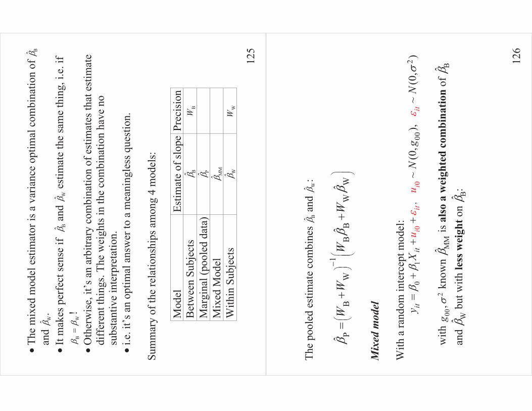
12
5
�
The
mix
ed m
odel
est
imat
or is
a v
aria
nce
optim
al c
ombi
natio
n of
�+
and
W�.
�It
mak
es p
erfe
ct se
nse
if �
+ a
nd
W� e
stim
ate
the
sam
e th
ing,
i.e.
ifW
��
+�
! �
Oth
erw
ise,
it’s
an
arbi
trary
com
bina
tion
of e
stim
ates
that
est
imat
e di
ffer
ent t
hing
s. Th
e w
eigh
ts in
the
com
bina
tion
have
no
subs
tant
ive
inte
rpre
tatio
n.
�i.e
. it’s
an
optim
al a
nsw
er to
a m
eani
ngle
ss q
uest
ion.
Su
mm
ary
of th
e re
latio
nshi
ps a
mon
g 4
mod
els:
Mod
el
Estim
ate
of sl
ope
Prec
isio
nB
etw
een
Subj
ects
� +
B
W
Mar
gina
l (po
oled
dat
a)P�
M
ixed
Mod
el
MM
�
W
ithin
Sub
ject
s W�
WW
12
6
The
pool
ed e
stim
ate
com
bine
s � +
and
W�:
1
PB
WB
BW
Wˆ
ˆˆ
WW
WW
��
��
��
��
��
��
��
��
�
��
��
Mix
ed m
odel
With
a ra
ndom
inte
rcep
t mod
el:
1
00
,00
~(0
,),
~(0
,)
ii
iti
itit
tu
uy
XN
gN
��
��
��
��
��
�
with
00
,g
�� k
now
n M
M�
is a
lso
a w
eigh
ted
com
bina
tion
of �
+
and
W� b
ut w
ith le
ss w
eigh
t on
� +:

12
7
MM
BB
00
B
//
Bet
wee
n-Su
bjec
tInf
orm
atio
nW
ithin
-Sub
ject
Info
rmat
ion
mon
oton
eTW
WT
g
fW
��
�
�
��
��
��
��
��
�
�
MM
� is
bet
wee
n W� a
nd
P�, i
.e. i
t doe
s bet
ter t
han
P� in
the
sens
e of
bei
ng c
lose
r to
W�bu
t is n
ot e
quiv
alen
t to
W�.
�
With
bal
ance
d da
ta
WM
MP
Pˆ
ˆˆ
ˆ�
��
��
��
�A
s 001
0T
g�
�
-
, M
MW
ˆˆ
��
-, s
o a
mix
ed m
odel
est
imat
es th
e
with
in e
ffec
t asy
mpt
otic
ally
in T
– w
hich
is th
e cl
uste
r siz
e N
OT
the
num
ber o
f clu
ster
s.
12
8
�
As
001T
g�
�
-
.,
MM
Bˆ
ˆ�
�-
. Thu
s the
mix
ed m
odel
est
imat
e fa
ils
to c
ontro
l for
bet
wee
n-su
bjec
t con
foun
ding
fact
ors.
Not
e th
at
this
doe
s not
cap
ture
the
who
le st
ory
beca
use
W� a
nd
B� a
re n
ot
inde
pend
ent o
f 00g. I
f 00
0g
� th
en
BW
��
�so
that
M
MB
W�
��
��
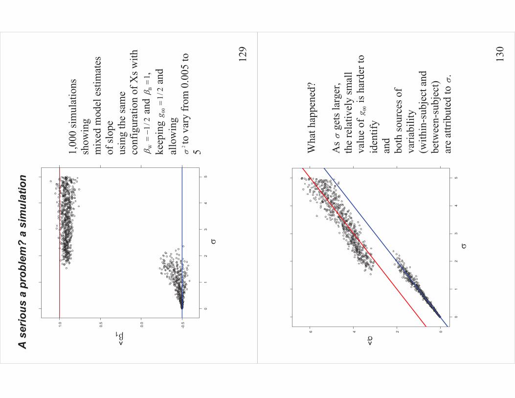
12
9
A s
erio
us a
pro
blem
? a
sim
ulat
ion
1,00
0 si
mul
atio
ns
show
ing
mix
ed m
odel
est
imat
es
of sl
ope
usin
g th
e sa
me
conf
igur
atio
n of
Xs w
ith
W1/
2�
��
and
B
1�
�,
keep
ing
001/
2g
� a
nd
allo
win
g
��to
var
y fr
om 0
.005
to
5
��
��1 -0.50.0
0.5
1.0
01
23
45
13
0
W
hat h
appe
ned?
A
s � g
ets l
arge
r,
the
rela
tivel
y sm
all
valu
e of
00g
is h
arde
r to
iden
tify
an
d
both
sour
ces o
f va
riabi
lity
(w
ithin
-sub
ject
and
be
twee
n-su
bjec
t)
are
attri
bute
d to
�.
��
�� 0246
01
23
45
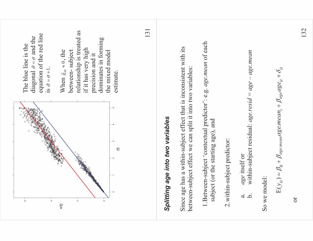
13
1
The
blue
line
is th
e di
agon
al �
��
and
the
equa
tion
of th
e re
d lin
e is
ˆ1
��
��
. W
hen
00ˆ0
g(
, the
be
twee
n- su
bjec
t re
latio
nshi
p is
trea
ted
as
if it
has v
ery
high
pr
ecis
ion
and
it do
min
ates
in fo
rmin
g th
e m
ixed
mod
el
estim
ate.
��
�� 0246
01
23
45
13
2
Split
ting
age
into
two
varia
bles
Si
nce
age
has a
with
in-s
ubje
ct e
ffec
t tha
t is i
ncon
sist
ent w
ith it
s be
twee
n-su
bjec
t eff
ect w
e ca
n sp
lit it
into
two
varia
bles
:
1.B
etw
een-
subj
ect ‘
cont
extu
al p
redi
ctor
’: e.
g. a
ge.m
ean
of e
ach
subj
ect (
or th
e st
artin
g ag
e), a
nd
2.w
ithin
-sub
ject
pre
dict
or:
a.
age
itsel
f or
b.w
ithin
-sub
ject
resi
dual
: age
.resi
d =
age
– a
ge.m
ean
So w
e m
odel
:
.E(
).
age
mea
nag
eit
iit
ity
agem
ean
age
��
��
��
��
�
or
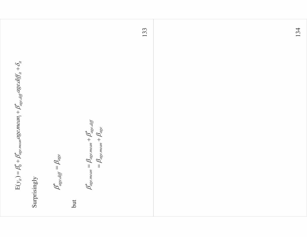
13
3
*
**
.0
.E(
).
.ag
emea
nit
iit
itag
ediff
yag
emea
nag
ediff
��
��
��
��
Su
rpris
ingl
y
*.
age
aged
iff�
��
bu
t
**
..
.
.
agem
ean
agem
ean
aged
iff
agem
ean
age
��
��
��
�
��
13
4
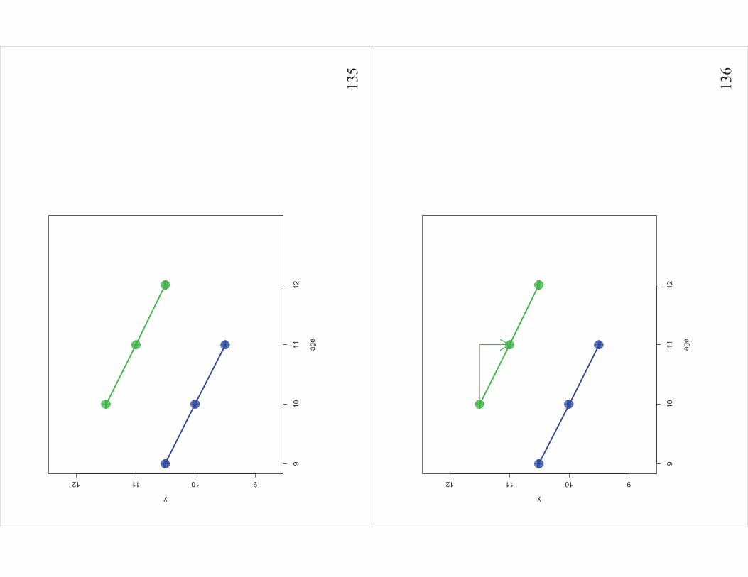
13
5
910
1112
9101112
age
y 13
6
910
1112
9101112
age
y
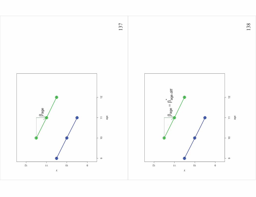
13
7
910
1112
9101112
age
y
��ag
e
13
8
910
1112
9101112
age
y
��ag
e�
� age.
diff
*
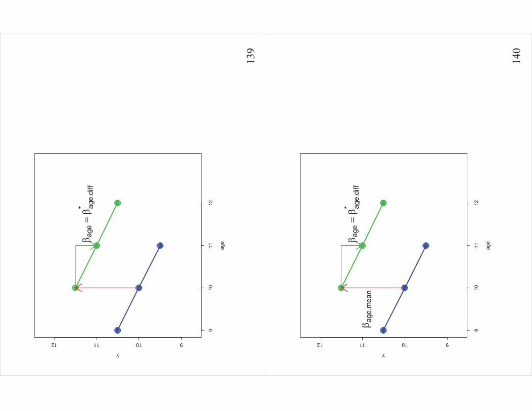
13
9
910
1112
9101112
age
y
��ag
e�
� age.
diff
*
14
0
910
1112
9101112
age
y
��ag
e�
� age.
diff
*
��ag
e.m
ean
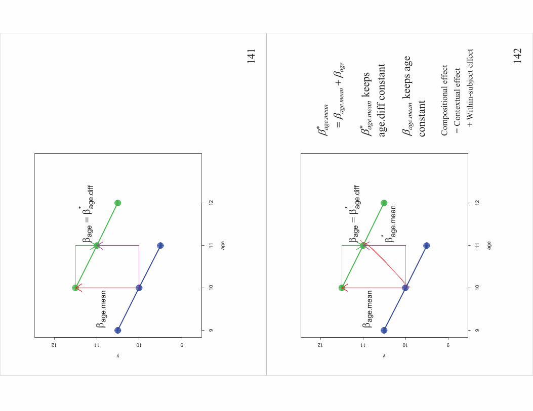
14
1
910
1112
9101112
age
y
��ag
e�
� age.
diff
*
��ag
e.m
ean
14
2
*
.
.
agem
ean
agem
ean
age
��
��
�
*
.ag
emea
n�
kee
ps
age.
diff
con
stan
t
.ag
emea
n�
kee
ps a
ge
cons
tant
910
1112
9101112
age
y
��ag
e�
� age.
diff
*
��ag
e.m
ean
��ag
e.m
ean
*
Com
posi
tiona
l eff
ect
= C
onte
xtua
l effe
ct
+ W
ithin
-sub
ject
effe
ct
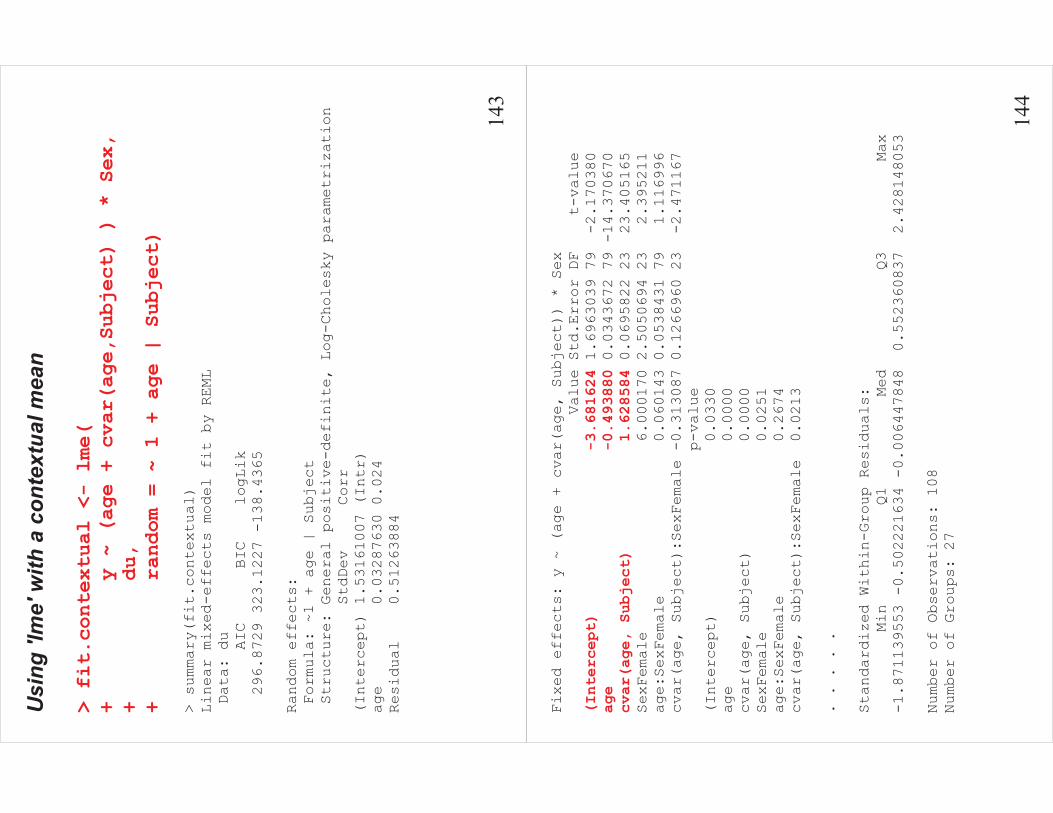
14
3
Usi
ng 'l
me'
with
a c
onte
xtua
l mea
n
> fit.contextual <- lme(
+ y ~ (age + cvar(age,Subject) ) * Sex,
+ du,
+ random = ~ 1 + age | Subject)
> summary(fit.contextual)
Linear mixed-effects model fit by REML
Data: du
AIC BIC logLik
296.8729 323.1227 -138.4365
Random effects:
Formula: ~1 + age | Subject
Structure: General positive-definite, Log-Cholesky parametrization
StdDev Corr
(Intercept) 1.53161007 (Intr)
age 0.03287630 0.024
Residual 0.51263884
14
4
Fixed effects: y ~ (age + cvar(age, Subject)) * Sex
Value Std.Error DF t-value
(Intercept) -3.681624
1.6963039 79 -2.170380
age -0.493880
0.0343672 79 -14.370670
cvar(age, Subject) 1.628584
0.0695822 23 23.405165
SexFemale 6.000170 2.5050694 23 2.395211
age:SexFemale 0.060143 0.0538431 79 1.116996
cvar(age, Subject):SexFemale -0.313087 0.1266960 23 -2.471167
p-value
(Intercept) 0.0330
age 0.0000
cvar(age, Subject) 0.0000
SexFemale 0.0251
age:SexFemale 0.2674
cvar(age, Subject):SexFemale 0.0213
. . . . .
Standardized Within-Group Residuals:
Min Q1 Med Q3 Max
-1.871139553 -0.502221634 -0.006447848 0.552360837 2.428148053
Number of Observations: 108
Number of Groups: 27
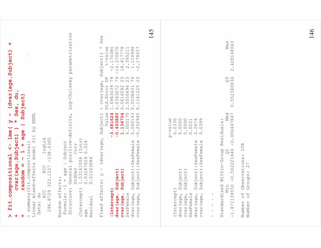
14
5
> fit.compositional <- lme( y ~ (dvar(age,Subject) +
+ cvar(age,Subject) ) * Sex, du,
+ random = ~ 1 + age | Subject)
> summary(fit.compositional)
Linear mixed-effects model fit by REML
Data: du
AIC BIC logLik
296.8729 323.1227 -138.4365
Random effects:
Formula: ~1 + age | Subject
Structure: General positive-definite, Log-Cholesky parametrization
StdDev Corr
(Intercept) 1.53161006 (Intr)
age 0.03287629 0.024
Residual 0.51263884
Fixed effects: y ~ (dvar(age, Subject) + cvar(age, Subject)) * Sex
Value Std.Error DF t-value
(Intercept) -3.681624
1.6963039 79 -2.170380
dvar(age, Subject) -0.493880
0.0343672 79 -14.370670
cvar(age, Subject) 1.134704
0.0616092 23 18.417778
SexFemale 6.000170 2.5050694 23 2.395211
dvar(age, Subject):SexFemale 0.060143 0.0538431 79 1.116996
cvar(age, Subject):SexFemale -0.252945 0.1161225 23 -2.178257
14
6
p-value
(Intercept) 0.0330
dvar(age, Subject) 0.0000
cvar(age, Subject) 0.0000
SexFemale 0.0251
dvar(age, Subject):SexFemale 0.2674
cvar(age, Subject):SexFemale 0.0399
. . . . .
Standardized Within-Group Residuals:
Min Q1 Med Q3 Max
-1.871139550 -0.502221640 -0.006447847 0.552360836 2.428148063
Number of Observations: 108
Number of Groups: 27

14
7
Sim
ulat
ion
Rev
isite
d 1,
000
sim
ulat
ions
us
ing
the
sam
e m
odel
s as t
he
earli
er si
mul
atio
n,
i.e.
the
sam
e co
nfig
urat
ion
of X
s w
ith
W1/
2�
��
and
B
1�
�,
keep
ing
001/
2g
�
and
al
low
ing
�
�to
var
y fr
om
0.00
5 to
5
��
��W�B -1.0
-0.50.0
0.5
1.0
01
23
45
14
8
Her
e a
mix
ed
mod
el is
use
d w
ith
mea
n ag
e by
su
bjec
t and
the
with
in-s
ubje
ct
resi
dual
of a
ge
from
mea
n ag
e.
��
��W�B -1.0
-0.50.0
0.5
1.0
01
23
45
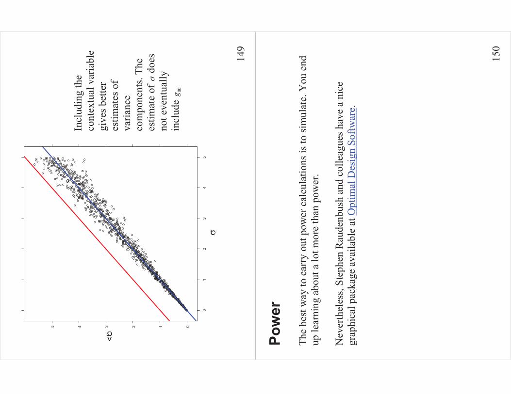
14
9
Incl
udin
g th
e co
ntex
tual
var
iabl
e gi
ves b
ette
r es
timat
es o
f va
rianc
e co
mpo
nent
s. Th
e es
timat
e of
� d
oes
not e
vent
ually
in
clud
e 00g
��
�� 012345
01
23
45
15
0
Pow
er Th
e be
st w
ay to
car
ry o
ut p
ower
cal
cula
tions
is to
sim
ulat
e. Y
ou e
nd
up le
arni
ng a
bout
a lo
t mor
e th
an p
ower
. N
ever
thel
ess,
Step
hen
Rau
denb
ush
and
colle
ague
s hav
e a
nice
gr
aphi
cal p
acka
ge a
vaila
ble
at O
ptim
al D
esig
n So
ftwar
e .
15
1
Som
e lin
ks
�
Ther
e is
a v
ery
good
cur
rent
bib
liogr
aphy
as w
ell a
s man
y ot
her
reso
urce
s at t
he U
CLA
Aca
dem
ic T
echn
olog
y Se
rvic
es si
te. S
tart
your
vis
it at
ht
tp://
ww
w.a
ts.u
cla.
edu/
stat
/sas
/topi
cs/re
peat
ed_m
easu
res.h
tm
�
Ano
ther
impo
rtant
site
is th
e C
entre
for M
ultil
evel
Mod
elin
g,
curr
ently
at t
he U
nive
rsity
of B
risto
l:
http
://w
ww
.cm
m.b
risto
l.ac.
uk/le
arni
ng-tr
aini
ng/m
ultil
evel
-m-
supp
ort/n
ews.s
htm
l
152
A fe
w b
ooks
�Pi
nhei
ro, J
ose
C. a
nd B
ates
, Dou
glas
M. (
2000
) Mix
ed-E
ffect
sM
odel
s in
S an
d S-
PLU
S. S
prin
ger
�
Fitz
mau
rice,
Gar
rett
M.,
Laird
, Nan
M.,
War
e, Ja
mes
H. (
2004
) Ap
plie
d Lo
ngitu
dina
l Ana
lysi
s, W
iley.
�A
lliso
n, P
aul D
. (20
05) F
ixed
Effe
cts R
egre
ssio
n M
etho
ds fo
r Lo
ngitu
dina
l Dat
a U
sing
SAS
, SA
S In
stitu
te.
�
Litte
ll, R
amon
C. e
t al.
(200
6) S
AS fo
r Mix
ed M
odel
s (2nd
ed.
), SA
S In
stitu
te.
�
Sing
er, J
udith
D. a
nd W
illet
t, Jo
hn B
. (20
03)
Appl
ied
Long
itudi
nal
Dat
a An
alys
is :
Mod
elin
g C
hang
e an
d Ev
ent O
ccur
renc
e. O
xfor
d U
nive
rsity
Pre
ss.
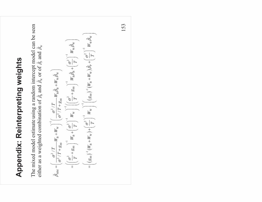
15
3
App
endi
x: R
eint
erpr
etin
g w
eigh
ts
The
mix
ed m
odel
est
imat
e usin
g a
rand
om in
terc
ept m
odel
can
be
seen
ei
ther
as a
wei
ghte
d co
mbi
natio
n of
�+ a
nd
W� o
r of
P� a
nd
W�
!
!
!
!
1
MM
BW
BB
WW
0000
11
11
1
00B
W00
BB
WW
11
11
00B
WW
00B
WP
//
ˆˆ
ˆ/
/
ˆˆ
ˆ
TT
WW
WW
Tg
Tg
gW
Wg
WW
TT
TT
gW
WW
gW
WT
T
��
��
��
�
��
��
��
��
�
��
�
��
��
��
��
��
�
��
��
��
��
��
��
��
��
��
��
��
��
��
��
��
��
��
��
��
��
��
��
��
��
��
��
��
��
��
��
��
��
��
��
��
��
��
��
��
�
��
��
�
��
��
�1
WWˆ
W�
��
��
��
��
��
��
�

![[ME] Multilevel Mixed Effects - Stata · PDF file[XT] Stata Longitudinal-Data/Panel-Data Reference Manual [ME] Stata Multilevel Mixed-Effects Reference Manual [MI] Stata Multiple-Imputation](https://static.fdocuments.in/doc/165x107/5a78a96c7f8b9a7b698e4b38/me-multilevel-mixed-effects-stata-xt-stata-longitudinal-datapanel-data-reference.jpg)