Long waves and short cycles in a model of

endogenous financial fragility

Soon Ryoo∗

October 4, 2010

Abstract

This paper presents a stock-flow consistent macroeconomic model in

which financial fragility in firm and household sectors evolves endoge-

nously through the interaction between real and financial sectors. Changes

in firms’ and households’ financial practices produce long waves. The Hopf

bifurcation theorem is applied to clarify the conditions for the existence of

limit cycles, and simulations illustrate stable limit cycles. The long waves

are characterized by periodic economic crises following long expansions.

Short cycles, generated by the interaction between effective demand and

labor market dynamics, fluctuate around the long waves.

Keyword cycles, long waves, financial fragility, stock-flow consistency

JEL classification E12, E32, E44

1 Introduction

A financial crisis hit the U.S and world economy in 2008. Giant financial in-stitutions have collapsed. Stock markets have tumbled, and exchange rates arein turmoil. Governments and central banks around the world have respondedby implementing bailout plans for troubled financial institutions and cutting in-terest rates to contain the financial panic, and expansionary fiscal packages are

∗Assistant Professor of Economics, Adelphi University, Garden City, NY 11530, USA,

email: sryoo@adelphi.edu. I would like to thank Peter Skott for his guidance, suggestions and

comments at all stages of this paper. I gratefully acknowledge helpful comments from two

anonymous referees, James Crotty, James Heintz, and participants in UMASS-New School

Graduate Workshop 2008. Any errors are mine. Published in Journal of Economic Behavior

and Organization. 2010. 74(3). 163-186

1

being pushed through to prop up aggregate demand. Hyman Minsky’s FinancialInstability Hypothesis offers an interesting perspective on these developments,which came after a long period of financial deregulation, rapid securitizationand the development of a range of new financial instruments and markets.1

According to Minsky’s financial instability hypothesis, a capitalist economycannot lead to a sustained full employment equilibrium and serious businesscycles are unavoidable due to the unstable nature of capitalist finance (Min-sky, 1986, 173). An initially robust financial system is endogenously turnedinto a fragile system as a prolonged period of good years induces firms andbankers to take riskier financial practices. During expansions, an investmentboom generates a profit boom but this induces investors and banks to adoptmore speculative financial arrangements. This is typically reflected in risingdebt finance, which eventually turns out to be unsustainable because the risingdebt changes cash flow relations and leads to various types of financial dis-tress. Minsky suggests that this kind of endogenous change in financial fragilitycan generate debt-driven long expansions followed by deep depressions (Minsky1964, 1995). In Minsky’s theory of long waves, short cycles fluctuate around thelong waves produced by endogenous changes in financial structure. Thus, thedistinction between short cycles and long waves is an important characteristicof Minsky’s cycle theory.

In spite of difficulties inherent in the formalization of Minsky’s theories,Minsky’s financial instability hypothesis has inspired a number of researchers tomodel the dynamic interaction between real and financial sectors. Taylor andO’Connell (1985), Foley (1986), Semmler (1987), Jarsulic (1989), Delli Gatti etal. (1994), Skott (1994), Dutt (1995), Keen (1995) and Flaschel et al. (1998,Ch.12) are early contributions. Recent studies include Setterfield (2004), Nasicaand Raybaut (2005), Lima and Meirelles (2007), and Fazzari et al. (2008).

This paper presents a stock-flow consistent model where firms’ and house-holds’ financial practices evolve endogenously through the interaction betweenreal and financial sectors. The interaction between changes in firms’ and house-holds’ financial practices produces long waves. The resulting long waves arecharacterized by periodic economic crises following long expansions. Short cy-cles, generated by the interaction between effective demand and labor marketdynamics, fluctuate around the long waves.

Compared to the previous literature, this paper has three distinct features:1Wray (2008), Cynamon and Fazzari (2008) and Crotty (2009), among others, provide per-

spectives on how shaky are the foundations of these ‘sophisticated’ developments in financial

markets.

2

First, the model in this paper is stock-flow consistent.2 Financial stocksare explicitly introduced and their implications for income and financial flowsare carefully modeled. In particular, unlike the previous studies listed above,capital gains from holding stocks are not assumed away and enter the definitionof the rate of return on equity. The rate of return on equity defined in thisway provides a basis of households’ portfolio decision. Firms’ and households’financial decisions jointly determine stock prices and the rate of return on equityin equilibrium. Thus, stock markets receive a careful treatment in this modeland play a central role in producing cycles.

Second, this paper pays attention to both firms’ and households’ financialdecisions. Minsky’s own account of financial instability tends to privilege thefirm sector as a source of fragility.3 Most previous studies follow this traditionand tend to neglect the role of households’ financial decisions in creating insta-bility and cycles. Some of the previous studies, including Taylor and O’Connell(1985), Delli Gatti et al. (1994), and Flaschel et al. (1998, Ch.12), do notsuffer from this kind of limitation but analyze households’ portfolio decision aswell. However, their neglect of the role of capital gains in households’ portfoliodecision makes it difficult to analyze the implication of households’ financialdecisions and stock market behavior for instability and cycles. In contrast tothese models, the model in this paper analyzes both households’ and firms’financial decisions. Capital gains and stock markets are considered explicitlyin a stock-flow consistent framework. The interactions between households andfirms turn out to be critical to the behavior of the system. The model consists oftwo subsystems: firms’ debt dynamics and households’ portfolio dynamics. Oneinteresting result of our analysis is that two stable subsystems can be combinedto produce instability and cycles in the whole system (See section 3). Thus,the resulting instability and cycles are genuinely attributed to the interactionbetween sectors rather than characteristics of one particular sector.

Lastly, existing Minskian models do not distinguish long waves from shortcycles and the periodicity of cycles in those models is ambiguous. Our modelis explicit in this matter. It produces two distinct cycles: long waves and short

2See Skott (1981), Godley and Cripps (1983) and Taylor (1985) for early introductions of

explicit stock-flow relations in a post-Keynesian / structuralist context. Simulation exercises

based on the stock-flow consistent framework have been flourishing since Lavoie and Godley

(2001-2).3Minsky’s neglect of the household sector is explained by his observation that “[H]ousehold

debt-financing of consumption is almost always hedge financing.” (1982, p. 32) This position,

however, has been challenged by some Minskian explanations of the sub-prime mortgage crisis

(e.g. Wray 2008 and Kregel 2008).

3

cycles. Long waves are produced by the interaction between firms’ and house-holds’ financial decisions, while short cycles are generated by the interactionbetween effective demand and labor market dynamics. The key idea underlyingMinsky’s financial instability hypothesis is that firms’, bankers’, and house-holds’ financial practices change endogenously. In the real world characterizedby complexity and uncertainty, agents’ financial practices are largely affectedby norms and conventions, which include borrowing and lending standards aswell as portfolio investors’ attitude to risks and uncertainty. Changes in thesenorms and conventions take time and tend to exhibit inertia. The long-termtrend in these elements would not be greatly disturbed by ups and downs dur-ing a course of short-run business cycles.4 Thus we interpret Minsky’s financialinstability hypothesis as a basis of long waves rather than a theory of short runbusiness cycles.5 Some of Minsky’s own writings support our interpretation. Forinstance, Minsky argues that (i) “The more severe depressions of history occurafter a period of good economic performance, with only minor cycles disturb-ing a generally expanding economy”(Minsky, 1995, p.85); (ii) the “mechanismwhich has generated the long swings centers around the cumulative changes infinancial variables that take place over the long-swing expansions and contrac-tions”(Minsky, 1964). To the best of our knowledge, our model is the first tointegrate an analysis of Minskian long waves with that of short cycles.

The analysis of the implications of financial behavior for instability and cy-cles in this paper complements a previous study on financialization and finance-led growth in Skott and Ryoo (2008) where the emphasis is on the effects ofchanges in financial behavior on long-run steady growth path with little atten-tion to questions of stability and fluctuations.

The rest of the paper is structured as follows. Section 2 sets up a stock-flow consistent model. Section 3 analyzes how the interaction between firms’and households’ financial practices produces long waves. Section 4 briefly in-troduces a model of short cycles into the current context. Section 5 combinesour model of long waves with the short-cycle model and provides simulationresults. Section 6 examines some alternative specifications. Section 7, finally,

4As pointed out by a referee, ‘financial behaviour in Minsky is clearly based on borrowing

and lending norms, and norms (like all institutions) are relatively inert and hence slow to

evolve. On this basis, it is surely more plausible to think that the drama of the financial

instability hypothesis is more likely to play itself out over the course of a long wave rather

than a single business cycle.’5It is surprising that Minsky’s theory of long waves has received little attention not only by

mainstream but also by heterodox economists. Palley (2009) recently called for understanding

Minsky’s theory through the lens of long term swings.

4

offers some concluding remarks.

2 Model

This section presents a model. Firms make decisions concerning accumulation,financing, and pricing/output; households make consumption and portfolio de-cisions; banks accept deposits and make loans. It is assumed that there areonly two types of financial assets - equity and bank deposits - and banks are theonly financial institution. It is assumed that the available labor force grows ata constant rate6 and long run growth is constrained by the availability of labor.

2.1 Firms

2.1.1 The finance constraint

Firms have three sources of funds in our framework: profits, new issue of equityand debt finance. Using these funds, firms make investments in real capital, payout dividends and make interest payments. Algebraically,

pI + Div + iM = Π + vN + M (1)

where I, Π, Div, M , and N are real gross investment, gross profits, dividends,bank loans and the number of shares, respectively. Bank loans carry the nominalinterest rate (i). p represents the price of investment goods as well as the generalprice of output in this one-sector model. All shares are assumed to have thesame price v.7

We assume that firms’ dividend payout is determined as a constant fractionof profits net of depreciation and real interest payments. The dividend payoutrate is denoted as 1 − sf and, consequently, sf represents firms’ retention rate.Thus, we have

Div = (1 − sf )(Π − δpK − rM) (2)

where K and δ are real capital stock and the rate of depreciation of real capital.r represents the real interest rate, r = i− p, where p is the inflation rate. Lavoieand Godley (2001-2002) and Dos Santos and Zezza (2007), among others, use thespecifications similar to (2) regarding firms’ retention policy. The real interestrate, rather than, the norminal rate, enters in the specification of dividend

6We assume that there is no technical progress but the model can easily accommodate

Harrod neutral technical progress7A dot over a variable refers to a time derivative (y = dy/dt).

5

payments, (2). Using the real interest rate in equation (2) may be justified iffirms treat the capital gain on existing debt from inflation (= pM) as a sourceof profit.8 Apart from the plausibility of this justification, specification (2)helps our analysis avoid possible complications due to the effect of inflation.Equation (2), in conjunction with the assumption of exogenous real interestrate (see section 2.2 below), makes dividend payments unaffected by a changein the inflation rate. This kind of inflation neutrality ceases to hold if the realinterest rate is replaced by the nominal rate in (2).9

New equity issue can be represented by the growth of the number of shares(N) or by the share of investment financed by new issues denoted as x. Skott(1989) and Foley and Taylor (2004) use the former and Lavoie and Godley(2001-2002) the latter. Two measures, however, are related to each other inthe following manner. It should be noted that x (and N) is not treated as aconstant parameter in this paper.

vNN = xpI (3)

Substituting (2) into (1), we get

pI − δpK = sf (Π − δpK − rM) + vNN + M(M − p) (4)

Scaling by the value of capital stock (pK), we have10

K ≡ g = sf (πuσ − δ − rm) + x(g + δ) + m + gm (5)

where π, u, and m are the profit share (π ≡ ΠpY ), the utilization rate (u ≡

YYF

, YF is full capacity output) and the debt-capital ratio (m ≡ MpK ). The

technical output/capital ratio, σ (≡ YF

K ), is assumed to be fixed. Equation (5)has a straightforward interpretation: firms’ investment (g) is financed by threesources: retained earnings, sf (πuσ − δ − rm), new equity issue, x(g + δ) andbank loans, m + gm. Given this finance constraint, firms’ financial behavior ischaracterized by sf , x (or N) and m. Most theories treat the rates of firms’retention and equity issue as parameters and debt finance as an accommodating

8This interpretation is provided by an anonymous referee.9In Fazzari et al.(2008), inflation plays a crucial role in generating a turning point of a

cycle: an investment boom leads to tightening labor market and increasing wage inflation.

The resulting price inflation raises the nominal interest rate, given the assumption that the

real rate is fixed. The increase in the nominal rate squeezes firms’ cash flow, which constrains

firms’ investment. Thus the inflation-cash flow-investment nexus is the key element of their

money non-neutrality result.10Equation (5) is obtained by dividing equation (4) by pK and then applying equation (3)

and some definitions ( IK

− δ ≡ g, ΠpK

≡ πuσ, MpK

≡ m, and M − p ≡ m + K).

6

variable (Skott 1989, Lavoie and Godley 2001-2002 and Dos Santos and Zezza2007). This paper assumes that the retention rate (sf ) is exogenous as in theabove literature but both the rate of equity issue (x or N) and the leverageratio m are endogenous. However, our way of treating equity finance and debtfinance is not symmetric.

Debt finance evolves through endogenous changes in firms’ and banks’ finan-cial practices which are directly influenced by the relationship between firms’profitability and leverage ratio (see section 2.1.2 below). With debt finance de-termined in this way, equity finance (x) serves as a buffer in the sense that oncethe other sources of finance − the retention and debt finance policies − andinvestment plans are determined, equity issues fill the gap between the fundsneeded for the investment plans and the funds available from retained earningsand bank loans. In this regard, equity finance is seen as a residual of firms’financing constraint.

Formally, for a given set of parameters sf , σ, δ and r, the trajectories ofendogenous variables g, π, u, m and m determine the required ratio of equityfinance to gross investment:

x =g − sf (πuσ − δ − rm) − m − gm

g + δ(6)

Our assumption that x is a residual suggests that firms cannot control theshare of investment financed by equity issues. In the present model, the tra-jectory of x is determined by a number of parameters including those describ-ing household consumption/portfolio behavior and banks’ loan supply decision.Firms’ desire to issue or buy back equities inconsistent with the trajectory of x

implied by the underlying parameters will be frustrated in the equity market.Our assumption regarding equity finance implies that x is treated as a fast

variable in our dynamical system, while the other methods of finance are mod-eled as an exogenous variable (sf ) or a state variable (m). As Figure 1 shows,in the U.S., the share of investment financed by equity issues - x - has substan-tially changed over time. The movement in the ratio appears to be very flexible.This was even more prominent when there were significant stock buybacks, i.e.the rate of net issue of equity was negative (x < 0). For instance, the share offixed investment financed by equity issues was nearly zero in 1982 but reached-42% in 1985. It then bounced back to a positive rate, 4.3% in 1991, and hitthe historical low, -71.5% in 2007. Firms have extensively used stock buybacksas a distributional mechanism since the 1980s, which, in our opinion, tends toincrease the flexibility of movements in the equity finance variable.

Increasing stock buybacks, in parallel to the reduction in the retention rate

7

-.8

-.6

-.4

-.2

.0

.2

1960 1970 1980 1990 2000

Figure 1: The Ratio of Net Issues of Equities to Fixed Investment (1952-2007)

Notes: Net issues of nonfinancial corporate equities divided by nonfarm nonfinancial

corporate (gross) fixed investment

Sources:Federal Reserve Board, Flow of Funds Accounts of the United States, Table

F.213 and Table F.102. Author’s calculation.

in the past decades, have received growing attention in the so-called financial-ization literature. Many studies on this issue have suggested that there havebeen structural changes in firms’ management and financial strategy in favorof shareholders. Most formal analyses of this subject have examined steadystate implications of changes in firms’ retention and equity finance policies, as-suming these changes in the policies can be represented by parametric shifts inthe corresponding exogenous variables (sf or x).11 Our specification of equityfinance as an endogenous variable provides another interesting interpretation ofincreasing stock buybacks. Equation (9) shows that increases in profitability(πuσ − δ − rm) and debt finance (m + gm) reduce the value of x, since theytend to relax firms’ budget constraints, other things equal. Given this relation,the observed shareholder value oriented management such as increasing stockbuybacks may be a consequence of a prolonged period of a debt driven profitboom. The present model, in fact, produces a result in which a long upswingdriven by rising firms’ debt finance and a stock market boom is accompaniedby a substantial decline in x.

There appears to be no reason to believe that the retention rate sf remainsconstant over time. The retention rate has gradually changed in the U.S. econ-

11See Skott and Ryoo (2008) for the related literature and a critical analysis of macroeco-

nomic implications of these developments.

8

omy. It was 75% in 1952 and had increased until it reached 88% in 1979. Theretention rate has fallen to about 70% in the past three decades (Skott andRyoo, 2008). This gradual pattern of the changes in the retention rate overthe long period may be best captured by modeling sf as a state variable alongwith other key state variables such as firm debt ratio and household portfoliocomposition. For instance, firms’ profit-interest ratio, the key determinant offirms’ liability structure (see section 2.1.2), may also affect firms’ desired re-tention rate by changing their perception of the margin of safety. Thus firms’high profitability relative to payment commitments may motivate them notonly to raise debt finance but also to pay out more dividends to shareholders.12

These kinds of laxer financial practices induced by strong profitability tend tostimulate aggregate demand and may contribute to the mechanism of a longexpansion because an increase in dividend income tends to raise consumptionthrough its direct effect on household income as well as its indirect effect onhousehold stock market wealth.13 In this setting, the two key developmentsassociated with financialization, falling sf and x, represent merely a phase of along cycle of endogenous changes in financial practices, as briefly suggested inSkott and Ryoo (2008). Although the endogeneity of the retention rate wouldproduce interesting results, we leave out this extension for the future research.sf will be assumed to be constant throughout this paper.

2.1.2 Endogenous changes in firms’ liability structure

Endogenous changes in firms’ liability structure, which are captured by changesin firms’ debt-capital ratio (m), are central in this paper, and a Minskian per-spective suggests that the debt-capital ratio evolves according to sustainedchanges in firms’ profitability relative to their payment obligations on debt.Changes in profitability that are perceived as highly temporary have only lim-ited effects on desired leverage. I, therefore, distinguish cyclical movements in

12This line of reasoning can be formalized as the following dynamic equation: sf =

ψ“

s∗f` ρT

rm

´

− sf

”

where ψ′(·) > 0, ψ(0) = 0 and s∗f′(·) < 0. s∗f (·) is the desired reten-

tion rate. This equation represents the sluggish adjustment of firms’ retention policy. The

present model, along with this dynamic equation, can generate the paths of sf and x declining

during a long expansion (our simulation results are available upon request).13Minsky acknowledged this kind of mechanism in the following remark: “During a run of

good times, the well-being of share owners improves because dividends to share ownership

increases and share prices rise to reflect both the higher earnings and optimistic prospects.

The rise in stockholder’s wealth leads to increased consumption by dividend receivers, which

leads to a further rise in profits. This relation between profits and consumption financed by

profit income is one factor making for upward instability.” (Minsky, 1986, 152)

9

profitability from the trend in average profitability and assume that changes inliability structure are determined by the trend of profitability.14

The perception of strong profitability relative to payment commitments dur-ing good years, Minsky argues, induces bankers and businessmen to adopt riskierfinancial practices which typically results in increases in the leverage ratio. Fol-lowing Minsky’s idea (Minsky, 1982, 1986), we assume that changes in the ratioof profit to debt service commitments drive changes in the debt structure. For-mally,

m = τ( ρT

rm

); τ ′(·) > 0 (7)

where ρT represents the trend rate of profit15and τ is an increasing function.During a period of good years when the level of profit is sufficiently high com-pared to interest payment obligations, firms’ and bankers’ optimism, reinforcedby their success, tends to make them adopt riskier financial arrangements whichinvolve higher leverage ratios. Moreover, a high profit level compared to debtservicing is typically associated with a low probability of default which helpsbankers maintain their optimism. The opposite is true when the ratio of profit tointerest payments is low. Firms’ failure to repay debt obligations - defaults andbankruptcies in the firm sector - put financial institutions linked to those firmsin trouble as well. This situation, which is often manifested in a system-widecredit crunch, tends to force firms and bankers to reduce firms’ indebtedness.

2.1.3 Accumulation

In general, capital accumulation is affected by several factors including prof-itability, utilization, Tobin’s q, the level of internal cash flows, the real interestrates and the debt ratio, but there is no consensus among theorists concerningthe sensitivity of firms’ accumulation behavior to changes in the various argu-ments. This paper follows a Harrodian perspective in which capacity utilizationhas foremost importance in firms’ accumulation behavior (Harrod, 1939). Theperspective assumes that firms have a desired rate of utilization. In the shortrun, the actual rate of utilization may deviate from the desired rate since firms’demand expectations are not always met and capital stocks slowly adjust. Ifthe actual rate exceeds the desired rate, firms will accelerate accumulation toincrease their productive capacity and if the actual rate is smaller than the de-sired rate, they will slow down accumulation to reduce the undesired reserve ofexcess productive capacity. However, in the long run, it is not reasonable to as-

14See section 3.1 for more discussion.15A definition of the trend rate of profit will be provided in section 3.

10

sume that the actual rate can persistently deviate from the desired rate becausecapital stocks can flexibly adjust to maintain the desired rate. This perspectivenaturally distinguishes the short-run accumulation function from the long-runaccumulation function.16

60

70

80

90

100

1950 1960 1970 1980 1990 2000

(a) Capacity Utilization: Total Index

60

70

80

90

100

1970 1975 1980 1985 1990 1995 2000 2005

(b) Capacity Utilization: Manufacturing (SIC)

Figure 2: Capacity Utilization. U.S (1948-2008)

Sources: Federal Reserve Board, Industrial Production and Capacity Utilization

A simple version of the long-run accumulation function can be written as

u = u∗ (8)

where u∗ is an exogenously given desired rate of utilization. (8) represents theidea that in the long run, the utilization rate must be at what firms want it tobe and capital accumulation is perfectly elastic so as to maintain the desiredrate. The strict exogeneity of the desired rate in (8) may exaggerate realitybut tries to capture mild variations of the utilization rate in the long-run. Forinstance, Figure 2 (a) and (b) plot the rate of capacity utilization in the U.S. forthe industrial sector and the manufacturing sector, respectively. The Hodrick-Prescott filtered series (dotted lines) are added to capture the long-run variationsin the utilization rate. The figures show that the degree of capacity utilizationis subject to significant short-run variations but exhibits only mild variationsaround 80% in the long-run.

In this paper, we use the long run accumulation function (8) to analyze longwaves: as long as we are interested in cycles over a fairly long period of time,

16This Harrodian perspective is elaborated in Skott (1989, 2008a, 2008b) in greater detail.

11

the assumption that the actual utilization rate is on average at the desired rateis a reasonable approximation.

This specification of long-run accumulation leaves out some possible deter-minants of investment, including the direct impact on investment of financialvariables such as cash flow and asset prices. Direct effects of this kind, whichhave been emphasized by the Minsky literature,17 are not necessary to generatelong waves in this paper. The key mechanism leading to long waves in thismodel is the effect of financial variables on aggregate demand. In the baselinemodel in sections 2-5, the demand effect of financial variables works primarilythrough households’ consumption demand. Section 6.2 extends the analysis toinclude a direct effect of financial variables on investment. This extension doesnot affect the qualitative conclusions.

The long run accumulation function (8) leaves the growth rate of capital, g,undetermined. The long-run average of g, however, will be approximately equalto the natural rate of growth, n, if the economy fluctuates around a steadygrowth path with a constant employment rate. As section 4 will show, thesystem of short cycles in the present model indeed produces the fluctuations of g

around n. Thus in the analysis of long waves, we assume that g is approximatedby its long run average n. Our analysis in section 4 will provide a justificationfor this procedure.

In the analysis of short cycles, u = u∗ will not be a reasonable assumptionany longer and it will be replaced by a short-run accumulation function (seesection 4).

2.2 Banks

It should be noted that equation (7) represents both bankers’ and firms’ fi-nancial practices. In other words, equation (7) is a reduced form of bank-firminteractions18 regarding the determination of firms’ liability structure. Thus

17The direct financial effects on investment play an important role in some Minskian models.

For instance, Taylor and O’Connell (1985) assumes that investment depends on the demand

price of capital assets, following Minksy’s two-price system approach. Delli Gatti et al. (1994)

and Fazzari et al. (2008) both assume that investment depends on cash flow in a nonlinear

way. Skott (1994) suggests that investment depends on hybrid variables such as ‘fragility’ and

‘tranquility’ which reflect financial conditions underlying investment decisions.18Banks and firms may map the profit-interest ratio to the debt ratio in a different manner.

For instance, banks’ willingness to lend, on the one hand, may be captured by mB = τB

` ρTrm

´

where τ ′B(·) > 0 and mB represents changes in firms’ leverage allowed by bankers. Firms’ loan

demand, on the other hand, may be represented by mF = τF

` ρTrm

´

where τ ′F (·) > 0 and mF

refers to changes in firms’ leverage implied by firms’ loan demand. If the actual movement of

the debt-capital ratio is assumed to be a non-decreasing function of τB(·) and τF (·), the τ(·)

12

bankers play important roles in shaping firms’ financial structure in this model.Banks’ role in the determination of firms’ debt structure has system-wide

implications as well. For a given profit-interest ratio, equation (7) determinesthe trajectory of the debt-capital ratio m. At any moment, the amount of loanssupplied to firms will be M = mpK. It is assumed that neither households norfirms hold cash, the loan and deposit rates are equal and there are no costsinvolved in banking. With these assumptions, the amount of loans to the firmsector must equal the total deposits of the household sector.

M = MH (9)

where MH represents households’ deposit holdings. Thus deposits are generatedendogenously through banks’ loan making process. Deposits created in this wayaffect households’ wealth, thereby changing the level of effective demand (Seesection 2.3 below).

Banks’ adjustment of the volume of loan supply during the course of cyclesmay have implications for their pricing behavior regarding interest rates. Forinstance, banks may have a tendency to raise loan interest rates as increasesin the volume of loans raise the probability of default risks. At the same time,financial innovations may offset this tendency by making the supply of financemore elastic.19 This consideration is likely more important in the long run thanin the short run. Monetary authority’s responses add more complications tothese developments. Its concern about inflation may or may not be dominatedby the development of its own euphoric expectations.

Precise modeling of banks’ pricing behavior, however, is beyond the scope ofthis paper. For the sake of simplicity, we assume that banks effectively controlthe real interest rate r. While the actual movements of interest rates are affectedby financial market conditions as well as various institutional changes and policyresponses, the assumption of perfectly elastic loan supply at a given interest rateappears to fit well with the focus of this paper on the endogenous adjustmentof the size of bank balance sheet especially in the longer run.

function can be defined as m = T`

τB

` ρTrm

´

, τF

` ρTrm

´´

≡ τ` ρT

rm

´

with T1 ≥ 0 and T2 ≥ 0. A

special case is obtained if the T -function is chosen as a lower envelope of τB(·) and τF (·).19“During periods of tranquil expansion, profit-seeking financial institutions invent and

reinvent “new” forms of money, substitutes for money in portfolios, and financial techniques

for various types of activity: financial innovation is a characteristic of our economy in good

times.” (Minsky, 1986, 178)

13

2.3 Households

Households receive wage income, dividends in return for their stock holdingsand interest income. Thus, household real disposable income denoted as Y H isgiven as: Y H = W+Div+rMH

p .Households hold stocks and deposits and household wealth is denoted as

NWH , where NWH = vNH+MH

p . Although the possibility of negative MH

cannot be excluded,20 this paper only concerns the case in which MH turns outto be positive. In other words, the household sector as a whole is in a net creditposition against the rest of the economy. This does not exclude the possibility inwhich some households are in a debtor position, but any such debt is assumedto be netted out for the household sector as a whole.21

Based on their income and wealth, households make consumption and port-folio decisions. We adopt a conventional specification of consumption function.(e.g. Ando and Modigliani, 1963)

C = C(Y H , NWH); CY H > 0 , CNW H > 0 (10)

For simplification, we assume that the function takes a linear form. We thenhave, after normalizing by capital stock and simple manipulations,

C

K= c1[uσ − δ − sf (πuσ − δ − rm)] + c2q (11)

where uσ − δ − sf (πuσ − δ − rm) is household income scaled by capital stockand Tobin’s q captures household wealth. c1 and c2 are household propensitiesto consume out of income and wealth. Note that the expression of householdincome, uσ − δ − sf (πuσ − δ − rm), implies that an increase in interest raiseshousehold income, other things equal. A dollar of interest increases householdincome by the same amount directly but decreases dividend income indirectlyby 100 × (1 − sf ) cents since it decreases firms’ net profits. The net effect willbe an increase in household income by 100× sf cents. If the real interest rate isconstant as in this paper, an increase in the debt ratio (m) tends to stimulateconsumption demand by raising household income.

In addition to consumption/saving decisions, households make portfolio de-cisions. We denote the equity-deposit ratio as α, where α ≡ vNH

MH .We assume that the composition of households’ portfolio is affected by their

views on stock market performance. Applying a Minskian hypothesis to house-hold behavior, it is assumed that during good years, households tend to hold a

20In this case, the absolute value of MH represents households’ net indebtedness against

the rest of the economy.21To introduce the implications of household debt, the model may have to be extended to

allow heterogeneity among households.

14

greater proportion of financial assets in the form of riskier assets. In our two-asset framework, equity represents a risky asset and deposits a safe asset. Thus,a rise in fragility during good years is captured by a rise in α. We introducea new variable z to represent the degree of households’ optimism about stockmarkets. We can normalize the variable z so that z = 0 corresponds to the statewhere households’ perception of tranquility is neutral and there is no changein α. Given this framework, the evolution of α is determined by an increasingfunction of z.

α = ζ(z); ζ(0) = 0, ζ ′(z) > 0 (12)

The next question is what determines households’ views about stock markets, z.It is natural to assume that household portfolio decisions, the division of theirwealth into stocks and deposits, will be affected by the difference between therates of return on stocks and deposits.

Our specification of the process in which households form their views onstock markets emphasizes historical elements in financial markets. Thus, thepast trajectories of rates of return on assets matter in the formation of z. Inaddition to the history of rates of return, the history of household portfolio de-cisions (α’s) may affect current households’ views on stock markets if currenthousehold portfolio decisions are largely influenced by their habits and con-ventions. As a crude approximation of this perception formation process, thefollowing exponential decay specification is introduced:

z =∫ t

−∞exp [−λ(t − ν)]κ (re

ν − r, αν) dν (13)

where re is the real rate of return on equity, κre ≡ ∂κ(re−r,α)∂re > 0 and κα ≡

∂κ(re−r,α)∂α < 0. In expression (13), κ (re

ν − r, αν) represents the informationregarding the state of asset markets at time ν. The higher the rate of return onequity relative to the deposit rate of interest, the more optimistic households’view on stock markets becomes (κre > 0). However, other things equal, ahigher proportion of their financial wealth in the form of stock holdings (highα) tempers the desire of further increases in equity holdings, i.e. κα < 0.

Information on asset markets at different times enters in the formation ofz with different weights. The term, exp [−λ(t − ν)], represents these weights,implying that a more remote past receives a smaller weight in the formation ofhouseholds’ perception of tranquility. Thus, λ may be seen as the rate of lossof relevance or loss of memory of past events. The higher λ, the more quickly

15

eroded is the relevance of past events.22 23

Differentiation of (14) with respect to t yields the following differential equa-tion:

z = κ (re − r, α) − λz (14)

Two dynamic equations (12) and (14), along with the equation describing theevolution of firms’ liability structure, (7), are essential building blocks for ourmodel of long waves. To proceed, we need to see how the rate of return onequity, re, is determined. re is defined as follows:

re ≡ Div + ΓvNH

=(1 − sf )(Π − δpK − rM) + (v − p)vNH

vNH(15)

where Γ is capital gains adjusted for inflation (Γ ≡ (v − p)vNH).The rate of return on equity is determined by stock market equilibrium.

Stock market equilibrium requires that the number of shares supplied by firmsequals that of shares held by households, N = NH , which implies N = NH in

22As pointed out by a referee, equation (13) implies that the weights on the history of α

are the same as those on re − r. This implicit assumption is not reasonable, but (13) can be

modified to allow different weights on the history of α and re − r in an additively separable

form. This modification increases the dimension of the resulting dynamical system, making

the qualitative analysis more cumbersome. The author, however, found that with introducing

the different weights an even wider range of parameter values successfully generate the cyclical

pattern proposed in this paper. This result is not surprising because the dimension of the

parameter set increases along with the change in the specification.23If the history of α does not matter for household portfolio decisions, (12) and (13) may

be modified as follows:

α = ζ(α∗ − α) (12a)

α∗ =

Z t

−∞exp [−λ(t − ν)]κ (re

ν − r) dν (13a)

where κ′(·) > 0 and α∗ is the desired equity-deposit ratio. (13a) tells us that households’

desired portfolio is determined by the trajectory of the difference between the rates of return

on equity and deposit. This desired ratio may not be instantaneously attained so that the

adjustment of the actual to the desired ratio takes time. (12a) represents this kind of lagged

adjustment of the actual equity-deposit ratio toward the desired ratio. In spite of different

interpretations, the two specifications, (12)-(13) and (12a)-(13a), are qualitatively similar. To

see this, let z ≡ α∗ − α. Then z = α∗ − α. Differentiating (13a) with respect to t, we have

α∗ = κ(re) − λα∗ = κ(re) − λ(α + z). Therefore, we can rewrite (12a) and (13a) to:

α = ζ(z) (12b)

z = κ(re) − λα − ζ(z) − λz (14a)

With (12b)-(14a), the qualitative analysis of the existence of a limit cycle is more complicated

than the case in the main text. To guarantee the existence of a limit cycle by way of the Hopf

bifurcation, more assumptions about the higher order derivatives of the underlying functions

are required.

16

terms of the change in the number of shares. Firms issue new shares wheneverretained earnings and bank loans fall short of the funds needed to carry theirinvestment plans. Thus firms’ finance constraint (1) implies that:

N =1v[pI + Div + iM − Π − M ] (16)

Simple algebra shows that capital gains can be expressed as follows:

Γ = (v − p)vNH = (α + m + K)vNH − vNH (17)

(α + m + K)vNH represents the total increase in the real value of stock marketwealth24 but some of the increase is attributed to the increase in the numberof shares (= vNH). To get the measure of capital gains, the latter should bededucted from the total increase.

Using N = NH , substituting (16) in (17) and plugging this result in (15),we get the new expression for re:

re =Π − iM + M + (α + m + K)vNH − pI

vNH(18)

Normalizing by pK, we get the expression for re as a function of π, u, m, m, α

and α:

re =πuσ − δ − rm + (1 + α)[m + mg)] + αm − g

αm(19)

≡ re(π, u, g,m, α, m, α) (20)

Substituting this expression in the dynamic equation (14), we have:

z = κ [re(π, u, g,m, α, m, α) − r, α] − λz (21)

(21) shows that households’ views of tranquility are affected by a number ofvariables and the relationship is complex. We consider several cases accordingto the property of (21) in section 3.

2.4 Goods market equilibrium

The equilibrium condition for the goods market is that CK + I

K = YK , and

the definition of q implies that q = (1 + α)m. Using these expressions, theequilibrium condition for the goods market can be written as:

c1[uσ − δ − sf (πuσ − δ − rm)] + c2(1 + α)m + g + δ = uσ (22)

24Note that α + m + K = v + N − p.

17

We take the profit share (π) as endogenous and the equilibrium value of π canbe found for given values of u, g, m and α. Explicitly, we have:

π =g − (1 − c1)(uσ − δ) + c2(1 + α)m + c1sf (δ + rm)

c1sfuσ(23)

≡ π(u, g,m, α) (24)

As u, g, m and α evolve over time, the profit share changes as well. The Har-rodian investment function adopted in this paper emphasizes a high sensitivityof investment to changes in the utilization rate. Specifically, it assumes thatinvestment is more sensitive than saving to variations in the utilization rate.This Harrodian assumption has an implication for the effect of changes in uti-lization on profitability: utilization has a positive effect on the profit share andthe magnitude will be quantitatively large.25 The large effect of changes in uti-lization on the profit share plays an important role in generating short cycles.(See section 4)

It is also readily seen that changes in the debt ratio and the equity-depositratio positively affect the profit share. Increases in the debt ratio or the equity-deposit ratio raise consumption demand though changes in disposable incomeor wealth, thereby increasing the profit share.26

2.5 Summary of the system of long waves

The model contains a number of behavioral relations. It may be useful tosummarize the key equations. The system of long waves is a three dimensionaldynamical system (7), (12) and (14), which consists of three state variables,m (firms’ liability structure: the debt-capital ratio), α (household portfoliocomposition: the equity-deposit ratio) and z (households’ confidence in stockmarkets).

m = τ( ρT

rm

), τ ′(·) > 0 (7)

α = ζ(z), ζ ′ > 0 (12)

z = κ (re − r, α) − λz, κre > 0; κα < 0 (14)

As long as the other two endogenous variables, ρT (the trend rate of cor-porate profitability) and re (the rate of return on equity), are determined as afunction of the state variables, the above dynamical system is closed.

25If∂(I/K)

∂u> (1 − c1)σ + c1sf πσ =

∂(S/K)∂u

, then ∂π∂u

=∂(I/K)

∂u−(1−c1)σ−c1sf πσ

c1sf uσ> 0.

26 ∂π∂m

=c1sf r+c2(1+α)

c1sf uσ> 0 and ∂π

∂α= c2m

c1sf uσ> 0

18

Goods market equilibrium determines the current rate of profit as a functionof u, m, and α. The trend rate of profit, ρT , is determined as a function of m

and α after adding the long run accumulation function u = u∗ (See section 3.1below). ρT is increasing in m and α.

ρT = ρT (m,α); ρT m > 0, ρT α > 0 (24A)

The rate of return on equity is determined by stock markets.

re = re(π(u∗, n,m, α), u∗, n,m, α, m, α) (20A)

where (20) is evaluated at u = u∗ and g = n. The rate of return on equityresponds to various arguments and its behavior appears to be complex. In anycase, m, α, and z determine re.

3 Long Waves

This section shows how endogenous changes in firms’ and households’ financialpractices generate long waves. Our model of long waves consists of two subsys-tems: one describes changes in firms’ liability structure and the other specifieschanges in households’ portfolio composition. Section 3.1 analyzes the evolu-tion of firms’ liability structure, assuming households’ portfolio composition isfrozen. Section 3.2 examines households’ portfolio dynamics, given the assump-tion that firms’ liability structure does not change. Section 3.3 combines twosubsystems and shows how long waves emerge from the interaction between twosubsystems.

3.1 Long-Run Debt Dynamics

This section analyzes the long-run evolution of firms’ debt structure. For con-venience, we reproduce equation (7).

m = τ( ρT

rm

)where τ ′(·) > 0 (7)

Regarding the shape of τ in (7), Minsky’s discussion suggests that the prosper-ity during tranquil years tends to induce firms and bankers to gradually raisethe leverage ratio; the rise in the leverage ratio, however, cannot be sustainedbecause it worsens the profit/interest relation. Minsky points out that the fi-nancial system is prone to crises as the ratio of profit to interest traverses acritical level (Minsky, 1995). The resulting systemic crisis may prompt a rapid

19

de-leveraging process. To capture this idea, we assume that τ ′(·) takes relativelysmall positive values within a narrow bound when ρT

rm is above a threshold level(good years), whereas it takes relatively large negative values when ρT

rm is be-low the threshold level (bad years). When falling profit/interest ratio passesthrough the threshold level, m sharply falls reflecting a rapid de-leveraging pro-cess. Thus, τ ′(·) is likely to be very large when ρT

rm = τ−1(0). Figure 3 reflectsthis assumption.

T

rm

m

()

1(0)

Figure 3: Debt-Capital Ratio and Profit-Interest Ratio

As briefly discussed in section 2.1.2, we use the trend rate of profit ρT asa basis of the evolution of firms’ liability structure. Behind equation (7) is theidea that firms’ liability structure evolves endogenously over time and that thekey determinant of the evolution is firms’ and banks’ perception of tranquility.The level of firms’ profit relative to payment commitments on liabilities is anindicator of firms’ performance and solvency status. Movements of the profitrate in general include both trend and cyclical components. It seems reasonableto assume that the long-run evolution of firms’ liability structure is primarilydetermined by the trend of the profit rate rather than the current profit rate.27

27This perspective is in line with Minsky’s statement that “[T]he inherited debt reflects

the history of the economy, which includes a period in the not too distant past in which the

economy did not do well. Acceptable liability structures are based on some margin of safety

so that expected cash flows, even in periods when the economy is not doing well, will cover

contractual debt payments”(Minsky, 1982, 65).

20

The driving force of the short-run cyclical movements in the current profitrate is changes in capacity utilization while the desired rate, u∗, provides agood approximation of the long-run average of actual rates of utilization. Thussetting the utilization rate at the desired rate, the short-run cyclical componentin the profit rate is effectively eliminated. In addition, the long-run average ofg can be approximated by n if the growth rate of capital fluctuates around thenatural rate. We then have:

ρT = π(u∗, n,m, α)u∗σ

=n − (1 − c1)(u∗σ − δ) + c2(1 + α)m + c1sf (δ + rm)

c1sf(25)

The trend rate of profit defined as (25) depends positively on the debt-capitalratio m and the equity-deposit ratio α (∂ρT

∂m > 0 and ∂ρT

∂α > 0). The profit-interest ratio, the key determinant of the liability structure, is written as

ρT

rm=

n − (1 − c1)(u∗σ − δ) + c2(1 + α)m + c1sf (δ + rm)c1sfrm

(26)

(26) implies that for a given value of α, the profit-interest ratio is uniquely de-termined by the debt-capital ratio m. Note that an increase in m raises thenumerator (profits) as well as the denominator (interest payments) of this ratio.Minsky’s implicit assumption that a rising debt ratio causes the profit-interestratio to deteriorate is satisfied only if the numerator rises slowly relative to thedenominator as m increases. Formally, the latter condition requires ∂ρT

∂m < ρT

m :the level of profits generated by a marginal increase in debt, due to the expan-sionary effect on aggregate demand of debt, falls short of the current profit-debtratio. In our linear specification of consumption function, this condition willhold if the ‘autonomous’ component of profits - the part of profits which is in-dependent of variations in m - is positive.28 Thus Minsky’s implicit assumptionis met if a sufficient level of demand, which is not entirely explained by thepositive effect of debt on demand, exists so that firms can make positive profitseven when m = 0.29 In the present model, the condition can be written in terms

28This proposition in the linear case can be generalized to any consumption function that

is homogenous of degree one with respect to household income and wealth. If consumption

function violates this homogeneity assumption, then the positiveness of ‘autonomous’ profits

does not guarantee the inverse relationship between m and ρTrm

. In particular, if the expan-

sionary effect of the debt ratio on profitability is excessively strong at a high level of m due

to the strong nonlinearity of consumption function, then the increase in m may increase the

profit-interest ratio.29The case in which m = 0 is just hypothetical especially in the present model where the

existence of debt is the basis of endogenous money creation. m = 0 amounts to the assumption

of non-monetary economy in the present context.

21

of parameters:n − (1 − c1)(u∗σ − δ) + c1sfδ > 0 (27)

Condition (27) may or may not be satisfied for plausible parameter values.30

For instance, if household marginal propensity consume c1 is relatively low, theinequality in (27) can be reversed. However, we will assume that condition(27) holds in order to keep track of the dynamic implications of the Minsky’sassumption of the inverse relationship between the profit-interest ratio and thedebt ratio.31

Using (7) and (26), m can be written as a function of m and α.

m = τ

(n − (1 − c1)(u∗σ − δ) + c2(1 + α)m + c1sf (δ + rm)

c1sfrm

)≡ F(m

−, α+)

(28)(28), along with the condition (27), implies that for any value of α, (i) F isdecreasing in m, (ii) there exists a unique value of the debt ratio m∗(α) such thatif m = m∗(α), m = 0, and (iii) m∗(α) depends positively on α, i.e. m∗′(α) > 0.By setting m to zero and solving for m, we obtain the algebraic expression form∗(α):

m∗(α) ≡ n − (1 − c1)(u∗σ − δ) + c1sfδ

[τ−1(0) − 1]c1sfr − c2(1 + α)(29)

It is straightforward from properties (i), (ii) and (iii) that (assuming α con-stant) our dynamic specification of Minsky’s financial instability hypothesis im-plies that firms’ debt structure monotonically converges to a stable fixed pointm∗. The intuition is simple. When the actual debt ratio (m) is lower thanm∗(α), the corresponding profit-interest ratio is greater than the threshold levelat which the debt ratio does not change. This will induce firms to raise thedebt ratio. The same kind of event will happen as long as m < m∗(α): m willeventually converge to m∗(α). The opposite will happen when the debt ratio isgreater than the critical level (m > m∗(α)).

Given assumption (28), a stable dynamics is inevitable in a one-dimensionalcontinuous time framework. Moving from a continuous to a discrete time frame-work may change the picture so that firms’ debt dynamics alone can produce

30To illustrate, suppose that n = 0.03, u∗ = 0.8, σ = 0.5, δ = 0.1 and sf = 0.75. Given

these parameter values, condition (27) requires that c1 > 0.72, which may or may not be met

in practice.31The implications of the violation of (27) are relatively lucid. For a given value of α, the

debt ratio will increase or decrease forever depending on the initial condition. The adjustment

of α tends to amplify this kind of unstable dynamics, which most likely yields exploding

trajectories.

22

long-run cyclical movements. In this paper, however, we explore another av-enue toward long waves by integrating firms’ debt dynamics into households’portfolio dynamics.

3.2 Household Portfolio Dynamics

The other subsystem of our model of long waves, which describes households’portfolio dynamics, consists of two dynamic equations:

α = ζ(z) (12)

z = κ (re − r, α) − λz (14)

Analogously to the analysis of firms’ debt dynamics, we are interested in thelong-run evolution of household portfolio decisions and, to simplify the analysiswe abstract from the effect of short-run variations in capacity utilization. Therate of return on equity evaluated at u = u∗ equals

re|u=u∗ =ρT (m,α) − δ − rm + (1 + α)[F(m,α) + mn] + ζ(z)m − n

αm(30)

Given this expression for re, equation (14) becomes

z = κ (re|u=u∗ − r, α) − λz ≡ G(m,α, z) (31)

(12), (28), and (31) constitute a three-dimensional dynamical system. To betterunderstand the mechanics of this three dimensional system, let us take a lookat the subsystem (12) and (31), assuming that m is fixed. By differentiating(31) with respect to α and z, the effects of α and z on z are given by:

Gα = κre

∂re

∂α+ κα S 0 (32)

Gz = κre

∂re

∂z− λ = κre

ζ ′

α− λ S 0 (33)

The effect of changes in α on z, Gα in (32), is decomposed into two parts. First,changes in α affect the rate of return on equity, which influences households’views on stock markets, κre

∂re

∂α . The effect of an increase in α on re, ∂re

∂α , canbe negative or positive in the steady state. Second, an increase in α mitigatesthe desire for further increases in equity holdings (κα < 0). Thus, the overalleffect depends on the precise magnitude of these two effects.

The effect of z on z is also unclear. On the one hand, an increase in house-holds’ optimism about stock markets accelerates stock holdings, which raisescapital gains and the rate of return on equity. The increase in re reinforces

23

their optimism (κre∂re

∂z > 0). On the other hand, the degree of optimism willerode at a speed of λ, holding re and α constant. Thus, the net effect is am-biguous.

Let JH be the Jacobian matrix evaluated at the fixed point of (12) and (31).The ambiguity of the signs of Gα and Gz yields four cases. Table 1 summarizesit.

Table 1: Classifying Fixed Points

Gz < 0 Gz > 0

Gα < 0Case I Stable

Tr(JH) < 0 and Det(JH) > 0

Case II Unstable

Tr(JH) > 0 and Det(JH) > 0

Gα > 0Case III Saddle

Tr(JH) < 0 and Det(JH) < 0

Case IV Saddle

Tr(JH) > 0 and Det(JH) < 0

A locally stable steady state in the subsystem is obtained when Gz and Gα

are both negative (Case I). In this case, λ is large relative to κre∂re

∂z , and κre∂re

∂α

is negative or, if positive, relatively small compared to the absolute value of κα.Thus, to get a locally stable steady state for households’ portfolio dynamics,the positive effect of changes in α and z on z via the rate of return on equityneeds to remain relatively small in the neighborhood of the steady state.

Moving from Case I, as λ gets smaller than κre∂re

∂z (Gz > 0), keeping thecondition Gα < 0, the steady state becomes locally unstable, yielding Case II.In this case, a high optimism further boosts households’ optimistic views onstock markets, creating destabilizing forces. The locally unstable steady state,along with nonlinearities of (12) and (31), can produce limit cycles as long asλ is not too small. Thus, in this case, households’ portfolio dynamics alone cangenerate persistent long waves.

If Gα > 0, i.e. κre∂re

∂α is larger than |κα|, then the fixed point of the house-holds’ portfolio dynamics becomes a saddle point, regardless of the sign of Gz

(Case III and IV). In both Case III and IV, a high level of equity holdings createsincreasing optimism (Gα > 0), making the steady state a saddle point. How-ever, Case IV is distinguished from Case III because it is an exceptional case:it turns out that the destabilizing force in Case IV is too strong to produce alimit cycle for the three dimensional full system ((12), (28), and (31)), whereas,in all other three cases I, II, and III, an appropriate choice of parameter valuescan produce a limit cycle for the full system. The next section analyzes the fullsystem of long waves.

24

3.3 Full Dynamics: Long Waves

We now put together firms’ debt and households’ portfolio dynamics and obtainthe following three dimensional dynamical system:

m = F(m,α) (28)

α = ζ(z) (13)

z = G(m,α, z) (31)

Let us first consider the Jacobian matrix of the system evaluated in the steadystate.

J =

Fm Fα 00 0 ζ ′

Gm Gα Gz

=

− + 00 0 +− +/− +/−

(34)

Gα and Gz are ambiguously signed but the partial derivative of G with respectto m is likely to be negative:

Gm = κre

∂re

∂m(35)

where

∂re

∂m=

[∂ρT

∂m m − ρT

]+ (1 + α)mFm + n + δ

αm2(36)

in the steady state. The sign of (36) may appear to be indeterminate: while∂ρT

∂m m − ρT is negative due to assumption (27) and (1 + α)mFm is negativesince Fm < 0, n + δ is positive. The discussion of the shape of τ(·) in section3.1, however, suggests that Fm is large in magnitude at the steady state growthpath.32 Thus, at the steady state, the negative terms in the numerator in (36)dominate, and the rate of return on equity will decrease as firms’ indebtednessincreases in the neighborhood of the steady state. Thus, we have Gm = κre

∂re

∂m <

0.We are interested in the conditions under which the system exhibits limit cy-

cle behavior. As sections 3.1 and 3.2 showed, the specification of firms’ financialdecisions, (28), leads to asymptotically stable dynamics, whereas households’portfolio dynamics ((12) and (31)) produces several cases in Table 1. Our ana-lytic result suggests that if households’ portfolio dynamics are neither stronglystabilizing nor strongly destabilizing, our baseline system of (12), (28) and (31)

32If τ ′(·) is large at ρTrm

= τ−1(0), the derivative of F(m, α) with respect to m is strongly

negative at m = m∗(α), i.e. |Fm| is large. In a limiting case where the de-leveraging process

is instantaneous at m∗(α), Fm → −∞.

25

tends to generate limit cycles. Our analysis of limit cycles is based on the Hopfbifurcation theorem. The Hopf bifurcation occurs if the nature of the systemexperiences the transition from stable fixed point to stable cycle as we graduallychange a parameter value of a dynamical system (Medio, 1992, section 2.7). wewill use λ as the parameter for the analysis of bifurcation.33 Proposition 134

provides the main results of our analysis of long waves:

Proposition 1 Consider the three dimensional system of (12), (28) and (31)and the Jacobian matrix (34) where the partial derivatives are taken at the steadystate values. Let

b ≡(|Fm|2 − ζ ′Gα) −

√(|Fm|2 − ζ ′Gα)2 + 4ζ ′|Fm||Gm|Fα

2|Fm|< 0

(I) (Case I and Case II) Suppose that Gz < min{|Fm|, ζ′|Gα|

|Fm|

}35 and

Gα < 0. Then a Hopf bifurcation occurs at λ = λ∗ ≡ κre∂re

∂z + |b|.As λ falls passing through λ∗, the system with a stable steady state losesits stability, giving rise to a limit cycle.

(II) (Case III) Suppose that Gz < 0 and 0 < Gα < min{

|Fm||Gz|ζ′ , Fα|Gm|

|Fm|

}.

Then a Hopf bifurcation occurs at λ = λ∗ ≡ κre∂re

∂z +|b|. As λ falls passingthrough λ∗, the system with a stable steady state loses its stability, givingrise to a limit cycle.

(III) (Case IV) Suppose that Gα > 0 and Gz > 0. Then the steady state isunstable. There exists no limit cycle by way of Hopf bifurcation.

Part (I) in the proposition suggests that the existence of a limit cycle re-quires at least three conditions: first, the mitigation effect of a high proportionof equity holdings on increasing optimism (|κα|) is sufficiently large so thatGα < 036; second, households’ optimistic or pessimistic view of stock marketsis not excessively persistent (Gz < min

{|Fm|, ζ′|Gα|

|Fm|

}); third, the rate of loss

33λ is particularly useful for the analysis not only because it is of obvious behavioral im-

portance but also because it provides analytic tractability due to the fact that changes in λ

do not affect steady state values.34The proof of Proposition I is found in Appendix A but the proof is concerned about only

the existence of a limit cycle. The computation of the coefficient that shows whether the

limit cycle is stable is very complicated and hard to interpret. Therefore, we extensively use

simulation exercises to observe the stability of cycles.35Note that Case I automatically satisfies the second condition since Gz < 0 in Case I.36Or the positive effect of changes in α on z via its effect on the rate of return on equity

should not be too large.

26

0.4 0.5 0.60.10

0.2

0.4

0.5

1

1.5

Debt Capital Ratio (m)

Equity/Deposit Ratio(

)

Household

Optimism

(z)

Long Expansion

Downturn

of relevance of past events (λ) should not be too large (λ < λ∗).37 The secondand third conditions imply that for the existence of a limit cycle, λ should beof appropriate magnitude:

κre

∂re

∂z− min

{|Fm|, ζ ′|Gα|

|Fm|

}< λ < κre

∂re

∂z+ |b| (37)

All of these conditions imply that to get a limit cycle, households’ portfoliodynamics should be neither strongly stabilizing nor strongly destabilizing.

One interesting aspect of Part (I) in Proposition I is that the interactionbetween two stable subsystems - firms’ debt and households’ portfolio dynamics- can generate an unstable steady state and a limit cycle (Case I). Thus, in thiscase, the source of the resulting long waves lies purely in the interaction betweenboth firm and household sectors. Figure 4 depicts the emergence of a limit cyclein this case in a three dimensional space. Figure 5 shows the trajectories of thedebt-capital ratio and the equity-deposit ratio in this case.

The debt-capital ratio and the equity-deposit ratio steadily increase duringa long boom.38 This expansion, however, is followed by a sharp fall in m andα, which have significant negative impacts on effective demand and trigger anabrupt downturn in the real sector (See section 4 below).

37If λ exceeds λ∗, then the system will be stabilized.38The functions and parameter values for this simulation, which are also used for the sim-

ulation in section 5, are found in Appendix B. A sufficiently long period of time (from t = 0

to t = 30000) is taken in all simulation exercises in this paper.

27

.30

.35

.40

.45

.50

.55

.60

.65

00 25 50 75 00 25 50

(a) Debt-Capital Ratio: Firrms

0.6

0.8

1.0

1.2

1.4

1.6

00 25 50 75 00 25 50

(b) Equity-Deposit Ratio: Households

Figure 5: Long Waves

Part (I) also covers Case II where the subsystem of households’ portfoliodynamics is unstable. As shown in 3.2, in Case II, portfolio dynamics alonecan create a limit cycle. Part (I) in the proposition suggests that the systemcan still have a limit cycle when the portfolio dynamics is combined with firms’debt dynamics. Then what is the implication of introducing the debt dynamicsinto portfolio dynamics? The qualitative analysis does not tell much aboutthe answer to this question. Numerical experiments, however, provide a casein which the amplitude and period of long waves get significantly larger as wemove from the 2D subsystem of portfolio dynamics to the full 3D system.

Part (II) in the proposition concerns Case III where the household portfoliosubsystem yields a saddle point steady state. Thus, this part of Proposition 1shows how stabilizing debt dynamics and households’ portfolio dynamics withsaddle property are combined to produce a limit cycle. Not surprisingly, notall saddle cases can generate a limit cycle. First, the destabilizing effect thatmakes the fixed point in the 2D household subsystem saddle − the magnitudeof Gα − should be mild: Gα < min

{|Fm||Gz|

ζ′ , Fα|Gm||Fm|

}. Second, Gz should

be negative. If it is positive (Gz > 0), the condition for the saddle point,Gα > 0, eliminates the possibility of the emergence of a limit cycle a la the Hopfbifurcation. Proposition 1-(III) makes this point. Intuitively, if both Gα > 0 andGz > 0 (Case IV), the portfolio dynamics in the household sector is excessivelydestabilizing in the sense that stabilizing forces in firms’ debt dynamics cannotcontain such a strong destabilizing effect.

To understand the mechanism behind the long waves, it is illuminating tocompare the full system with the subsystem of debt dynamics. As seen in

28

A

C

B

m

T

rm

-1(0)

Figure 6: The relationship between the debt-capital ratio and the profit-interest

ratio

section 3.1, with households’ portfolio composition (α) fixed, the debt-capitalratio (m) monotonically converges to its steady state value m∗(α). The mainreason for this convergence was the inverse relation between m and ρT

rm : a risingdebt-capital ratio causes firms’ profit-interest ratio to deteriorate for any givenα. However, once households’ portfolio composition evolves endogenously, thiskind of strict inverse relationship breaks down because changes in α also affectρT

rm .Figure 6 illustrates this point, where the horizontal dotted line represents

the threshold level (= τ−1(0)) of the profit-interest ratio that makes m zero. Inthe area above the horizontal line, the debt-capital ratio increases and in thearea below the line, it decreases. With α held fixed, the movement along thecurve AB is not possible since for any given α, a rise in m is incompatible witha rise in ρT

rm . However, increases in α fueled by households’ optimism during anexpansion have a positive effect on the profit-interest ratio by raising aggregatedemand. Thus, from A to B, the economy experiences increases in both α and

29

m.39 However, households’ optimistic views on stock markets eventually fadeas both m and α increase. As a result, the negative effect of a rise in the debtratio starts to be dominant at some point and the profit-interest ratio beginsfalling (point B). Because the profit-interest ratio is still above the thresholdlevel, the debt ratio keeps increasing and the profit-interest ratio falls alongthe curve BC. When the profit-interest ratio passes through point C, the debt-capital ratio starts to fall. When the economy reaches point A, a new cyclebegins.

m

m

Expansion m m

Contraction m m

t

m,m

A

B

D

C

Figure 7: Actual and Desired Debt Ratios

Figure 7 depicts the same story from a slightly different angle. The solidline plots a trajectory of the actual debt-capital ratio over time and the dottedline a trajectory of the desired debt ratio (m∗ ≡ m∗(α) in (29)). For a givenvalue of α, the debt dynamics, (28), implies that the actual debt ratio m tendsto gravitate toward the desired ratio m∗(α). However, when α changes, thedesired ratio becomes a moving target of the actual ratio. From this view, aperiod of expansion (contraction) is the time when the actual ratio is below(above) the desired ratio, i.e. m < m∗ (m > m∗) and consequently the actual

39The positive effect of the rise in α on the profit-interest ratio dominates the negative effect

of the rise in m and consequently the profit-interest ratio also increases during this period.

30

debt ratio is increasing (decreasing). In words, a stock market boom (rising α)tends to raise the tolerable level of the debt-capital ratio which the actual ratiois chasing. When the relation between m and m∗ is reversed, a long downturnbegins (See point C in Figure 7). The endogeneity of the desired debt ratio (orthe acceptable liability structure) plays a pivotal role in Minsky’s explanationof boom and bust cycles.

As Minsky put it, “[B]orrowing and lending take place on the basis of mar-gins of safety.”(Minsky, 1982, 74) The ratio of gross profits to cash paymentobligations on debts is “the fundamental margin of safety.” The profit-interestratio, ρT

rm , in the present model represents this fundamental margin of safety,and the τ -function the relation between the liability structure and the marginof safety. The nonlinearity of the τ -function plays a crucial role in producingthe asymmetric pattern of long waves. During good times, the economy oper-ates to the right of τ−1(0) in Figure 3, where the debt ratio increases due tothe sufficient margin of safety. Slow increases in the debt ratio tend to erodethe margin of safety but the asset market boom more than offsets this negativeeffect initially. Thus ρT

rm increases and the economy moves further to the right.Since m changes much more slowly in the region to the right of τ−1(0) thanto the left of it, the economy will stay in that region much longer than in theother. As the stock market boom subsides and begins to fall, the margin ofsafety starts to decline quickly since the stock market development reinforcesthe negative effect of rising debt ratio on the margin of safety. As the marginof safety is eroded and traverses the barrier given by τ−1(0), the systemic cri-sis can occur along with a detrimental de-leveraging process. The asymmetricshape of the τ -function represents this kind of rapid de-leveraging mechanism:m is very large when ρT

rm < τ−1(0). The margin of safety would be recoveredquickly due to the sharp decline in m if the stock market condition remainedtranquil. The reality is that stock market crashes exacerbate the problem ofthe malfunctioning banking system. It will take some time until the economyreaches the turning point, bypassing the point of τ−1(0) from the left to theright. Thus our τ function shows how the fundemantal margin of safety andfirms’ liability structure interacts to creat a Minskian boom-bust cycle.

4 A Model of Short Cycles

The model of long waves in section 3.3 can be combined with a model of shortcycles. In our analysis of long waves, the degree of capacity utilization is setat its long run average. However, when it comes to short cycles, the utilization

31

rate can deviate from the desired rate due to falsified demand expectations andslow adjustment of capital stocks. Thus we introduce the following short-runaccumulation function:

K ≡ g = ϕ(u − u∗); ϕ′(·) ≫ 0, ϕ(0) = n (38)

The strong positive effect of utilization on accumulation in (38) embodiesthe Harrodian accelerator principle.

By plugging (38) into (23), we derive the profit share that ensures goodsmarket equilibrium, which depends positively on u, m, and α.

π = π(u+, m

+, α+) (39)

Regarding firms’ pricing/output decisions, this paper adopts a Marshallian ap-proach elaborated in Skott (1989). The Keynesian literature often assumes thatprices are sticky while output adjusts instantaneously and costlessly to absorbdemand shocks but the Marshallian approach assumes the opposite. Outputdoes not adjust instantaneously due to a production lag and substantial ad-justment costs.40 In this framework, fast adjustments in prices and the profitshare establish product market equilibrium for a given level of output. In acontinuous-time setting, sluggish output adjustment can be approximated byassuming that output is predetermined at each moment and that firms choosethe rate of growth of output, rather than the level of output. Then outputgrowth is determined by comparing the costs and benefits involved in the out-put adjustment which in turn are determined by the labor market conditionsand the profit signal in the goods market, respectively. Thus we can formulate:

Y = h(π, e); hπ > 0, he < 0 (40)

where e is the employment rate. A higher profitability induces firms to expandoutput more rapidly whereas the tightened labor market gives firms negativeincentives to expand production.41 Assuming a fixed-coefficient Leontief tech-nology, Y = min{σK, νL}, the employment rate can be expressed as: e = Y/ν

L,

where ν is constant labor productivity and L is available labor force whichexponentially grows at a constant natural rate n. From this definition,

e = Y − n (41)

40For instance, increases in production and employment require substantial search, hiring

and training costs. Hiring or layout costs include not only explicit costs but also hidden costs

such as a deterioration in industrial relations and morale.41For more details about the behavioral foundation of (39), see Skott (1989, Ch.4).

32

The definition of u yields:u = Y − K (42)

Putting together (38) - (42), we get the following system of short cycles.

u = h(π(u+,m

+, α+), e

−) − ϕ(u

+− u∗) (43)

e = h(π(u+,m

+, α+), e

−) − n (44)

When m and α are fixed, the system of (43) and (44) exhibits essentially thesame dynamic properties as Skott (1989). As Skott shows, under plausibleassumptions, the system of (43) and (44) ensures the existence of a steadygrowth equilibrium and the steady state is locally asymptotically unstable unlessthe negative effect of employment on output expansion is implausibly large.Once the boundedness of the trajectories is proved, the system (43) and (44)will generate a limit cycle a la the Poincare-Bendixson theorem (See Skott 1989,Appendix 6C for the proof).

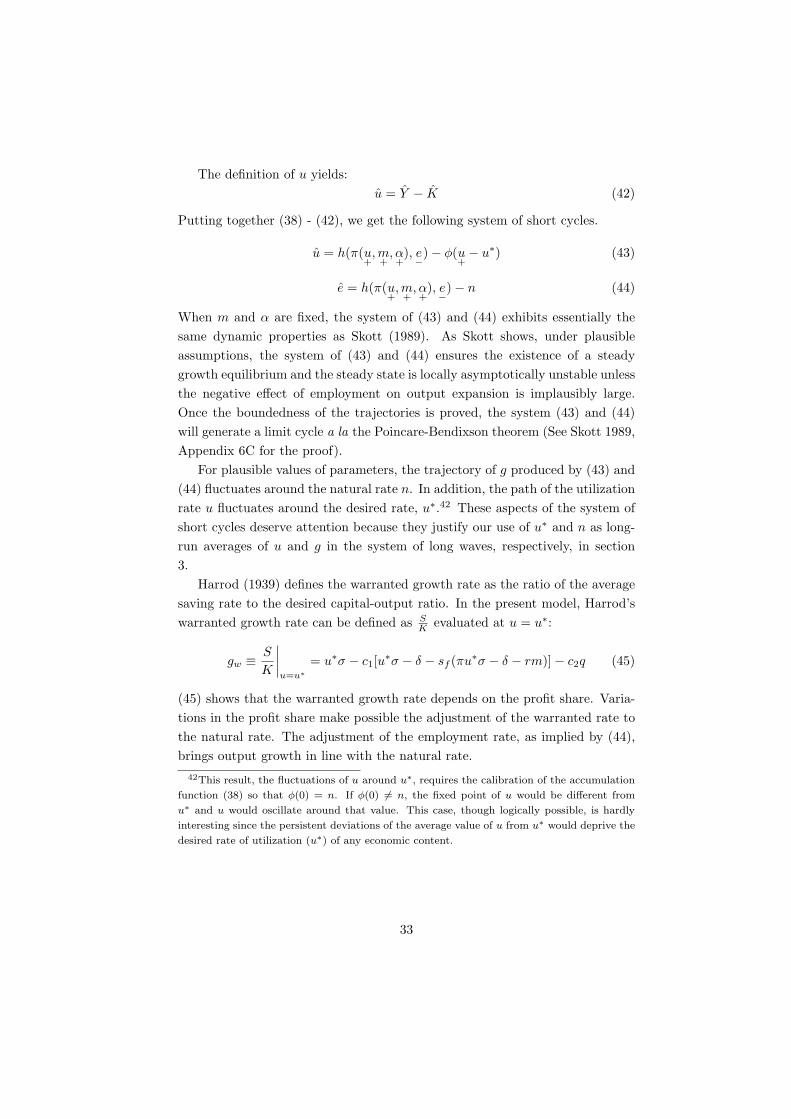
For plausible values of parameters, the trajectory of g produced by (43) and(44) fluctuates around the natural rate n. In addition, the path of the utilizationrate u fluctuates around the desired rate, u∗.42 These aspects of the system ofshort cycles deserve attention because they justify our use of u∗ and n as long-run averages of u and g in the system of long waves, respectively, in section3.

Harrod (1939) defines the warranted growth rate as the ratio of the averagesaving rate to the desired capital-output ratio. In the present model, Harrod’swarranted growth rate can be defined as S

K evaluated at u = u∗:

gw ≡ S

K

∣∣∣∣u=u∗

= u∗σ − c1[u∗σ − δ − sf (πu∗σ − δ − rm)] − c2q (45)

(45) shows that the warranted growth rate depends on the profit share. Varia-tions in the profit share make possible the adjustment of the warranted rate tothe natural rate. The adjustment of the employment rate, as implied by (44),brings output growth in line with the natural rate.

42This result, the fluctuations of u around u∗, requires the calibration of the accumulation

function (38) so that ϕ(0) = n. If ϕ(0) = n, the fixed point of u would be different from

u∗ and u would oscillate around that value. This case, though logically possible, is hardly

interesting since the persistent deviations of the average value of u from u∗ would deprive the

desired rate of utilization (u∗) of any economic content.

33

5 Putting the pieces together: Long Waves and

Short Cycles

This section puts all of the elements together in order to integrate long waveswith short cycles and presents our simulation results.43 Our full model of longwaves and short cycles is a five dimensional dynamical system that consists of(12), (28), (31), (43), and (44). We have seen that (12), (28), and (31) providea model of long waves, whereas (43) and (44) generate a mechanism of shortcycles. 44

A

B

Downturn

Long Expansion

e

(b) Long Waves and Short Cycles(a) Short Cycles without Long-Run Dynamics

m, fixed

e

Figure 8: Comparison

As seen in section 4, if m and α are fixed, (43) and (44) produce a limitcycle under plausible conditions. It can be shown that the resulting limit cycleexhibits a clockwise movement in e-u space, or alternatively, in e-π space. Fig-ure 8 (a) presents an example of the limit cycle on the e-π space. The system of(12), (28) and (31), however, generates long waves of the debt-capital ratio (m)and the equity-deposit ratio (α), which are represented in Figure 5. As m and α

change endogenously, the limit cycle in Figure 8 (a) breaks down and the clock-wise movement of e and π spirals up to the northeast or down to the southwest,

43Parameter values and functions used for this simulation are available in Appendix B. The

simulation in this section is based on Case I in Table 1. Simulation results in other cases are

available upon request.44By using (25) as our definition of trend profitability based on u = u∗, the system of long

waves becomes independent of that of short cycles, while the latter depends on the former.

Issues regarding the relation between long and short cycles will be discussed in section 6.1.

34

depending on the direction of changes in m and α. Figure 8 (b) illustrates this.The upward spiral from A to B represents a long expansion driven by increasesin the debt-capital ratio and the equity-deposit ratio, whereas the downwardspiral from B to A an economic downturn prompted by sharp decreases in m

and α.

.0

.1

.2

.3

.4

.5

.6

00 25 50 75 00 25 50

(a) Profit Share

-.1

.0

.1

.2

.3

00 25 50 75 00 25 50

Gross Rates Net Rates

(b) Profit Rate

0.84

0.88

0.92

0.96

1.00

00 25 50 75 00 25 50

(c) Employment Rate

-.6

-.4

-.2

.0

.2

.4

00 25 50 75 00 25 50

(d) Rate of Return on Equity

Figure 9: Simulation Paths I

During each long expansion, the profit share exhibits a strong upward move-ment with mild cyclical fluctuations around the trend (Figure 9 (a)). The similarpattern characterizes the movements in the profit rates (Figure 9 (b)). Duringcrises, the rate of profit net of depreciation and interest payment (πuσ−δ−rm)tumbles even to negative rates. Changes in the debt structure have large im-pacts on the real sector performance through its effect on profitability. Thisis prominently shown in the behavior of the employment rate (Figure 9 (c)).Figure 9 (d) depicts a trajectory of the rate of return on equity. During longbooms, the rate of return on equity is strong and sound on average but during

35

crises, it suddenly drops to significantly negative rates.

.76

.77

.78

.79

.80

.81

.82

.83

.84

00 25 50 75 00 25 50

Hodrick-Prescott Filtered Series

(a) Capacity Utilization

-.02

.00

.02

.04

.06

00 25 50 75 00 25 50

Hodrick-Prescott Filtered Series

(b) Output Growth

-.02

.00

.02

.04

.06

00 25 50 75 00 25 50

Hodrick-Prescott Filtered Series

(c) Capital Accumulation

.68

.72

.76

.80

.84

00 25 50 75 00 25 50

(d) Ration of Consumption to Disposable Income

Figure 10: Simulation Paths II

Figure 10 (b) shows the growth rate of output where the Hodrick-Prescottfiltered trend is added.45 A financial sector induced crisis triggers a deep re-cession in the real sector which is reflected in the negative growth rates duringperiodic deep downturns. Capacity utilization and capital accumulation followthe pattern similar to that of output growth(Figure 10 (a) and (c)). Figure10 (d), finally, plots the ratio of consumption to household income. The seriesfollows the basic long waves/short cycles patten as shown in the profit shareand the employment rate but the movement in the consumption/income ratiois noticeably smooth compared to other simulated series.46

45The filtered series is only for illustrative purpose since it simply smoothes the original

series and it does not adequately capture asymmetric features and structural breaks in the

original series.46The long run behavior of consumption is closely related to the movement in house-

hold net worth to income ratio: CY H = c1Y H+c2NW H

Y H = c1 + c2NW H

Y H where NW H

Y H =

36

6 Alternative specifications

6.1 Direct effect of financial variables on investment

This subsection introduces the direct effect of financial variables on investment.In our Harrodian framework, this can be achieved by assuming desired uti-lization depends on financial variables. Financial variables may affect firms’desired capital stock by changing the cost of finance. Two financial variablesare of interest: Tobin’s q and cash flow, denoted as c. An increase in q tendsto reduce the cost of finance, thereby increasing firms’ desired capital stock.This kind of traditional cost of capital channel may be captured by the inverserelationship between desired utilization and q. In imperfect capital markets, thelevel of cash flow may also affect the cost of finance because internal funds arecheaper than external finance due to the existence of external finance premiumor the financial accelerator (e.g. see Fazzari et al. 1988; Bernanke, Gertler, andGilchrist,1996). Thus imperfect capital markets may yield the inverse relation-ship between desired utilizatin and cash flow. Based on these considerations,the long-run accumulation function (8) is rewritten as

u = u∗(q, c), u∗q ≡ ∂u∗

∂q< 0, u∗

c ≡ ∂u∗

∂c< 0, (46)

and the short-run accumulation function (38) is correspondingly modified to

g = ϕ (u − u∗(q, c)) , ϕ′(·) > 0, ϕ(0) = n (47)

where c = sf (πuσ − δ − rm) and q = (1 + α)m.Using equations, (11) and (47), the goods market equilibrium condition be-

comes:c1(uσ − δ − c) + c2q + ϕ (u − u∗(q, c)) + δ = uσ (48)

As long as |u∗c | = c1

ϕ′ , π can be written as a function of u, m and α with the aidof the implicit function theorem (Note that c is a function of π). In the newshort-run investment specification, the expression for the Harrodian assumption- investment is more sensitive than saving to variations in the utilization rate -is slightly modified to

∂(I/K)∂u

= ϕ′ · (1 + |u∗c |sfπσ) > (1 − c1)σ + sfπσ =

∂(S/K)∂u

(49)

Changes in the actual rate of utilization directly affect accumulation throughthe flexible accelerator mechanism. In addition, changes in actual utilization

(1+α)muσ−sf (πuσ−δ−rm)

.

37

influence accumulation indirectly because they change the level of cash flow,which affect the desired utilization rate. The indirect effect reinforces the directeffect. Assuming the Harrodian condition (49), it can be shown that if the effectof cash flow on desired utilization is not too large, i.e. |u∗

c | < c1ϕ′ ,47 the profit

share, π, is increasing in u, m and α.

π = π∗(u,m, α), π∗u > 0, π∗

m > 0, π∗α > 0 (50)

Furthermore, the examination of the partial derivatives of π with respectto its arguments reveals that the positive effects of u, m, and α on π are allstronger in the new investment specification than in the case of the constantrate of desired utilization. The main intuition for this result is that changes inu, m, and α have additional demand effects since increases in these variablestend to reduce desired utilization, thereby stimulating accumulation.

Trend profitability is obtained by substituting u = u∗(q, c) into (48). Wethen have:

c1(u∗(q, c)σ − δ − c) + c2q + n + δ = u∗(q, c)σ (51)

where c = sf (ρ∗T − δ − rm) and q = (1 + α)m. If |u∗c | < c1

(1−c1)σ,48 then the

trend rate of profit can be expressed as an increasing function of α and m:

ρ∗T = ρ∗T (m, α), ρ∗Tm > 0, ρ∗Tα > 0 (52)

It can be shown that as in the short run case, the new specification of long-run accumulation, (46), strengthens the expansionary effects of m and α on ρT

in the original specification.In this paper, the key characteristics of the trend rate of profit (25) and the

actual profit share (39) are their positive dependence on m and α. It has beenshown that these properties of ρT - and π- functions remain unaffected by intro-ducing the direct effect of financial variables on firms’ accumulation behavior.Moreover, these expansionary effects get stronger as the direct financial effectson investment are allowed.

Simulation results are qualitatively similar to the baseline model but the newspecification implies that desired capacity utilization gradually declines duringa long boom and suddenly jumps as a crisis hits the economy. Not surprisingly,

47This condition implies that saving is more sensitive than investment to variations in π.

This condition is critical for the stability of (ultra) short-run product market equilibrium.

Apart from the stability issue, the violation of this condition produces an empirically implau-

sible result such as the profit share decreasing in capacity utilization.48Assuming the Harrodian assumption holds in the case of constant desired utilization,

|u∗c | < c1

ϕ′ implies |u∗c | < c1

(1−c1)σ.

38

the deviation of the actual rate of utilization from the desired rate exhibits apattern similar to that in the case of the fixed rate of desired utilization.

6.2 Relation between long waves and short cycles

In section 5, long waves were strictly separated from short cycles because trendprofitability defined as (25) was not affected by changes in the actual utilizationrate. This formal separability should not disguise the important role of shortcycles in producing long waves. The long waves in the present model are gen-erated based on the assumption that u∗ and n provide a good approximationof the long run averages of actual movements in utilization and accumulation.This assumption can be justified only when the system of short cycles actuallyproduces the fluctuations of u and g around u∗ and n. The system of shortcycles in the present model does this job, thereby making firms’ and bankers’long-term expectations consistent with the actual trajectories of the economy.If the system of short cycles fails to produce the fluctuations of u and g aroundu∗ and n, this consistency requirement will not be satisfied. In sum, the sys-tem of short cycles is not subsidiary but it plays a pivotal role in providingfirms and bankers with an anchor of their long-term expectations of corporateprofitability.

The assumption that trend profitability is not affected by acutal utilization,however, appears to be strong. The formal separation of long waves from shortcycles ceases to hold once changes in the actual capacity utilization rate affecttrend profitability. Then the question is, how robust are the analytic results inthe previous sections once this strict separation is relaxed?

Any reasonable definition of trend profitability requires a conceptual distinc-tion between the long run and the short run components of actual movementsin the profit rate. The actual profit rate is defined as ρ ≡ π(u,m, α)uσ. Theactual rate of profit is affected by changes in financial practices (m or α) andchanges in the utilization rate (u). The approach taken in the earlier part of thispaper treats changes in u as entirely short-run cyclical factors while it considerschanges in m and α as long-run factors. This was the basis of the definitionof trend profitability in equation (25), but one may argue that changes in theutilization rate contain both trend and cyclical components. For instance, sup-pose that the trend utilization rate, denoted as uT , follows an averaging processgiven by (53).

uT = µ(u − uT ) (53)

where µ represents the adjustment speed. This adjustment process yields an

39

alternative measure of trend profitability, (ρAT ):

ρAT ≡ π(uT ,m, α)uT σ (54)

The constant desired utilization rate (u∗) is replaced by the trend utilizationrate (uT ). If the long-run evolution of firms’ liability structure is determined byρA

T rather than ρT , then the system of long waves is no longer strictly separablefrom that of short cycles because the actual utilization rate affects the trendutilization rate, which in turn influences trend profitability in (54).

Analytic results depend on the value of µ. Two polar cases of (53) are ofinterest: (i) µ → 0 with uT = u∗ and (ii) µ → ∞. It is readily seen thatcase (i) is equivalent to the approach taken in the earlier part of this paper,which leads to the strict separability of long waves from short cycles. Case (ii),µ → ∞, implies that the trend utilization rate instantaneously adjusts to theactual rate and thus trend profitability is always equal to the actual profit rate.Thus case (ii) undermines the conceptual distinction between trend and actualprofitability.

If the value of µ is small enough, one can get a sufficiently smooth trend ofcapacity utilization and trend profitability given by (54). The analytic resultsbased on the assumption that u = u∗ in the previous sections remain unaffectedif µ is sufficiently small. The trend rate of utilization gradually adjusts itselftoward actual utilization but the link between the trend rate of utilization andthe desired rate will not break down because the interaction between the goodsmarket and the labor market in the short cycle system will prevent actual uti-lization from diverging away from desired utilization indefinitely. Thus both uT

and u will fluctuate around u∗.

7 Conclusion

The U.S. economy is going through a deep recession triggered by the biggestfinancial crisis since the Great Depression. A Minskian perspective suggeststhat the explanation of this crisis should be found in endogenous changes infinancial fragility.

This study has modeled a Minskian theory of long waves. The model clarifiesthe underlying mechanism of endogenous changes in financial fragility and theinteraction between real and financial sectors. At a theoretical level, the studyprovides a promising way of integrating two types of instability principles: Min-sky’s Financial Instability Hypothesis and Harrod’s Instability Principle. Whileboth principles provide a source of cycles, they have distinct frequencies and

40

amplitudes in this model. The Minskian instability hypothesis creates longwaves and the Harrodian instability principle produces short cycles. The limitto the upward trend created by Minskian instability is imposed by financial cri-sis, while explosive trajectories implied by Harrodian instability are containedby stabilizing labor market dynamics.49 When two principles are combined intoa coherent stock-flow consistent framework, the proposed pattern of long wavesand short cycles emerges.

A purely mathematical model of this kind may clarify the logic of interactionsbut clearly has many limitations. The depth of the current crisis and the timeneeded to initiate a new cycle depend on institutional and policy dimensions.Minsky devotes a large part of his analysis to the institutional and historicaldevelopments of financial markets and policy responses. Thus, the patterns oflong waves are heavily affected by these elements. The full account of long wavesand crises is possible only when one takes a serious look at these dimensions.

Disregarding the historical contingencies of actual movements, it may beuseful to extend the model in a number of directions. First, it may be desirableto give a more detailed treatment to banks’ behavior. The assumption of thefixed real interest rate may be too simple to characterize banks’ pricing behav-ior over the course of cycles. The financial sector may have to be disaggregatedto address the issues regarding securitization, a key aspect of the recent finan-cial crisis. Bankers’ perception of tranquility is possibly affected by their ownprofitability. Next, this paper did not explore the implications of households’indebtedness. Instead, it has focused on an increasing share of stocks (riskierasset) in households’ financial wealth as an indicator of increasing fragility inthe household sector. It would be interesting to see the effect of the introductionof the evolution of household debt into the model. Third, the proposed modelis inflation neutral in the sense that the decisions on real quantities such asinvestment, consumption and output expansion are made with no reference toinflation and the banking sector holds the real interest rate at a constant level.In some account of Minskian ideas (e.g Fazzari et al., 2008), changes in the in-flation rate play an important role. Finally, the assumption of a closed economyin this paper is another major limitation. Unfettered international capital flows,in contrast to the belief of its proponents, have created growing instability andglobal imbalances (Blecker, 1999). Several authors suggest that Minsky’s theory

49The following quote from Minsky (1995, 84) is suggestive: “As reasonable values of the

parameters of the endogenous interactions lead to an explosive endogenous process, and as

explosive expansions and contractions rarely occur, then constraints by devices such as the

relative inelasticity of finance or an inelastic labor supply need to be imposed and be effective

in generating what actually happens.”

41

can be extended to an international context (e.g. Wolfson, 2002 and Arestis andGlickman, 2002), but few attempts have been made to formalize the ideas andto propose precise mechanisms behind them. Addressing these issues is left forfuture research.

References

[1] Ando, A., Modigliani, F., 1963. The life cycle hypothesis of saving: Aggre-gate implications and tests. American Economic Review 53, 55-84.

[2] Arestis, P., Glickman, M., 2002, Financial crisis in Southeast Asia: dis-pelling illusion the Minskian way. Cambridge Journal of Economics 26,237-260.

[3] Bernanke, B., Gertler, M., Gilchrist, S., 1996. The Financial acceleratorand the flight to quality. The Review of Economics and Statistics 78, 1-15.

[4] Blecker, R., 1999. Taming Global Finance: A better Architecture forGrowth and Equity. Washington DC: Economic Policy Institute.

[5] Crotty, J., 2009. Structural causes of the global financial crisis: A criti-cal assessment of the ‘new financial architecture’. Cambridge Journal ofEconomics 33, 563-580.

[6] Cynamon, B. Z., Fazzari, S. M., 2008. Household debt in the consumer age:Source of growth-risk of collapse. Capitalism and Society 3.

[7] Delli Gatti, D. Gallegati, M., Gardini, L., 1994. Complex dynamics in asimple macroeconomic model with financing constraints. In: Dymski, G.,Pollin, R. (Eds.). New Perspectives in Monetary Macroeconomics: Ex-plorations in the Tradition of Hyman Minsky. Ann Arbor: University ofMichigan Press. 51-77.

[8] Dos Santos, C.H., Zezza, G., 2007. A simplified, benchmark, stock-flowconsistent Post-Keynesian growth model. Metroeconomica 59, 441-478.

[9] Dutt, A.K., 1995. Internal finance and monopoly power in capitalisteconomies: A reformulation of Steindl’s growth model. Metroeconomica46, 16-34.

[10] Fazzari, S., Ferri, P., Greenberg, E., 2008. Cash flow, investment, andKeynes-Minsky cycles. Journal of Economic Behavior and Organization65, 555-572.

42

[11] Fazzari, S.M., Hubbard, R. G., Peterson, B.C., 1988. Financing constraintsand corporate investment. Brookings Papers on Economic Activity 1, 141-195.

[12] Flaschel, P., Franke, R., Semmler, W., 1998. Dynamic Macroeconomics:Instability, Fluctuation, and Growth in Monetary Economies. The MITPress.

[13] Foley, D. K., 1986. Liquidity-profit rate cycles in a capitalist economy.Journal of Economic Behavior and Organization 8, 363-376.

[14] Foley, D. K., Taylor, L., 2006. A heterodox growth and distribution model.In: Salvadori, N. (Ed). Economic Growth and Distribution: On the Natureand Causes of the Wealth of Nations. Edward Elgar. 75-99.

[15] Godley, W., Cripps, F., 1983. Macroeconomics, Oxford: Fontana and Ox-ford University Press.

[16] Harrod, R., 1939. An Essay in Dynamic Theory. The Economic Journal 49,14-33.

[17] Jarsulic, M., 1989. Endogenous credit and endogenous business cycle. Jour-nal of Post Keynesian Economics 12, 35-48

[18] Keen, S., 1995. Finance and economic breakdown: modeling Minsky’s “fi-nancial instability hypothesis.” Journal of Post Keynesian Economics 17,607-635

[19] Kregel, J., 2008. Minsky’s cushions of safty: Systemic risk and the crisis inthe U.S. subprime mortgage market. Public Policy Brief No.93A, The LevyEconomics Institute of Bard College.

[20] Lavoie, M., Godley, W., 2001-2002. Kaleckian models of growth in a co-herent stock-flow monetary framework: a Kaldorian view. Journal of PostKeynesian Economics 24, 277-311.

[21] Lima, G. T., Meirelles, A., 2007. Macrodynamics of debt regimes, financialinstability and growth. Cambridge Journal of Economics 31, 563-580.

[22] Medio, A., 1992. Chaotic Dynamics: Theory and Applications to Eco-nomics. Cambridge University Press.

43

[23] Minsky, H.P., 1964. Longer waves in financial relations: Financial factorsin the more severe depressions. The American Economic Review, Papersand Proceedings of the Seventy-sixth Annual Meeting of the AmericanEconomic Association 54, 324-335.

[24] Minsky, H.P., 1982. Can “It” Happen Again? - Essays on Instability andFinance. M.E. Sharpe, Inc.

[25] Minsky, H. P., 1986. Stabilizing an Unstable Economy. Yale UniversityPress.

[26] Minsky, H.P., 1995. Longer waves in financial relations: Financial factorsin the more severe depressions II. Journal of Economic Issues 29, 83-96.

[27] Nasica, E., Raybaut, A., 2005. Profits, confidence, and public deficits:modelling Minsky’s institutional dynamics. Journal of Post Keynesian Eco-nomics 28, 135-155.

[28] Palley, I. T. 2009, A theory of minsky super-cycles and financial crises,05-2009, IMK at the Hans Boeckler Foundation, Macroeconomic PolicyInstitute.

[29] Semmler, W., 1987. A macroeconomic limit cycle with financial pertuba-tions. Journal of Economic Behavior and Organization 8, 469-495.

[30] Setterfield, M., 2004. Financial fragility, effective demand and the businesscycle. Review of Political Economy 16, 207-223.

[31] Skott, P., 1981. On the ‘Kaldorian saving function’. Kyklos 34, 563-81.

[32] Skott, P., 1989. Conflict and Effective Demand in Economic Growth. Cam-bridge: Cambridge University Press.

[33] Skott, P., 1994. On the modelling of systemic financial fragility. In: Dutt,A. K. (Ed). New Directions in Analytic Political Economy. Aldershot, UKand Brookfield, US, Edward Elgar. 49-76.

[34] Skott, P., 2008a. Theoretical and empirical shortcomings of the Kaleckianinvestment function. Working paper series 2008-14, Department of Eco-nomics, University of Massachusetts Amherst.

[35] Skott, P., 2008b. Growth, instability and cycles: Harrodian and Kaleck-ian models of accumulation and income distribution. Working paper series2008-14, Department of Economics, University of Massachusetts Amherst.

44

[36] Skott, P., Ryoo, S., 2008. Macroeconomic implications of financialisation.Cambridge Journal of Economics 32, 827-862.

[37] Taylor, L., 1985. A stagnationist model of economic growth. CambridgeJournal of Economics 9, 383-403.

[38] Taylor, L., O’Connell, S.A., 1985. A Minsky crisis. The Quarterly Journalof Economics 100, 871-885.

[39] Wolfson, M. H., 2002. Minsky’s thoery of financial crises in a global context.Journal of Economic Issues 36, 393-400.

[40] Wray, L. R., 2008. Financial markets meltdown: What can we learn fromMinsky. Public Policy Brief No.94, The Levy Economics Institute of BardCollege.

45

Appendix A: Proof of Proposition 1

To prove the existence of a limit cycle for the system of (12), (28), and (31),we need to show that the Jacobian matrix (34) evaluated at (m(λ), α(λ), z(λ),λ), where (m(λ), α(λ), z(λ)) is a fixed point of the system,50 should have thefollowing properties:

• The Jacobian matrix has a pair of complex conjugate eigenvalues β(λ) ±θ(λ)i such that β(λ∗) = 0, θ(λ∗) = 0, and β′(λ∗) = 0 and no othereigenvalues with zero real part exist at (m(λ∗), α(λ∗), z(λ∗) , λ∗)

where λ∗ is a Hopf bifurcation point.To apply the above condition for the Hopf bifurcation to the current context,

we will use the fact that the Jacobian matrix will have a negative real root anda pair of pure imaginary roots if and only if:

(R1) Tr(J) = Fm + Gz < 0

(R2) J1 + J2 + J3 = FmGz − ζ ′ · Gα > 0

(R3) Det(J) = −ζ ′ · (FmGα − FαGm) < 0

(R4) −Tr(J)(J1 + J2 + J3) + Det(J) = −(Fm + Gz)(FmGz − ζ ′ · Gα) − ζ ′ ·(FmGα − FαGm) = 0

Let us denote the eigenvalues of the Jacobian matrix as µ(λ) and β(λ)±θ(λ)i.

Proof of (I) Suppose that Gα < 0. Then (R3) is always met. In orderto satisfy (R1) and (R2), we should have Gz < min

{|Fm|, ζ′|Gα|

|Fm|

}. (R4) is

quadratic in Gz. (R4) can be rewritten as:

a1G2z + a2Gz + a3 = 0 (A1)

where

a1 ≡ −Fm > 0

a2 ≡ −(F2m − ζ ′Gα) S 0

a3 ≡ ζ ′FαGm < 0

Solving (A1) for Gz, we obtain one negative and one positive real roots. Letus select the negative root51, which is given as:

50Note that in our case the fixed point is independent of the value of λ.51It can be shown that the positive root is irrelevant for the analysis.

46

b ≡(|Fm|2 − ζ ′Gα) −

√(|Fm|2 − ζ ′Gα)2 + 4ζ ′|Fm||Gm|Fα

2|Fm|< 0 (A2)

Since Gz = κre∂re

∂z −λ, the value of λ that satisfies (R4) is: λ = κre∂re

∂z + |b|. Let

λ∗ ≡ κre∂re

∂z + |b|. We have shown that if Gz < min{|Fm|, ζ′|Gα|

|Fm|

}and λ = λ∗,

then the Jacobian matrix has a negative real root and a pair of imaginary roots:µ(λ∗) < 0, β(λ∗) = 0, and θ(λ∗) = 0. To prove λ∗ is indeed the bifurcationpoint, we still need to show that β′(λ∗) = 0. To prove β′(λ∗) = 0, let us use thefollowing fact:

µ(λ) + 2β(λ) = Fm + Gz

2µ(λ)β(λ) + β(λ)2 + θ(λ)2 = FmGz − ζ ′ · Gα

µ(λ)[β(λ)2 + θ(λ)2] = −ζ ′ · (FmGα − FαGm)

Totally differentiating both sides with respect to λ, we get 1 2 02β(λ) 2[µ(λ) + β(λ)] 2θ(λ)

[β(λ)2 + θ(λ)2] 2µ(λ)β(λ) 2µ(λ)θ(λ)

µ′(λ)

β′(λ)θ′(λ)

=

−1|Fm|

0

(A3)

The right hand side of (A3) is obtained using the fact that ∂Gz

∂λ = −1 and λ

does not affect all other partial derivatives than Gz. Evaluating (A3) at λ = λ∗,we have: 1 2 0

0 2µ(λ∗) 2θ(λ∗)θ(λ∗)2 0 2µ(λ∗)θ(λ∗)

µ′(λ∗)

β′(λ∗)θ′(λ∗)

=

−1|Fm|

0

Solving this for β′(λ∗), we finally get:

β′(λ∗) =2µ(λ∗)θ(λ∗)|Fm| − 2θ(λ∗)3

4µ(λ∗)2θ(λ∗) + 4θ(λ∗)3< 0 since µ(λ∗) < 0

Thus, β′(λ∗) is strictly negative.

Proof of (II) Suppose that Gα > 0 and Gz < 0. Then (R1) is always satisfied.To meet (R2) and (R3), we need Gα < min

{|Fm||Gz|

ζ′ , Fα|Gm||Fm|

}. The rest of the

proof is essentially the same as that of (I).

47

Proof of (III) Routh-Hurwitz necessary and sufficient conditions for the localstability of a three dimensional system are (R1), (R2) and (R3) with replacingthe equality in (R4) by the inequality: −Tr(J)(J1 + J2 + J3) + Det(J) > 0.Suppose that Gα > 0 and Gz > 0. Then (R2) is always violated and the fixedpoint is unstable. At the same time, since (R2) is not met, it is impossible toget a limit cycle a la the Hopf bifurcation.

Appendix B: Functions and Parameter Values in

Simulation

g = γ0 + γ1u (B1)

I

K= g + δ (B2)

Y = h(π, e) = h0 +h1

1 + exp[−h2(π + h3 ln(h4 − e) + h5))](B3)

m = τ( ρT

rm

)= τ0 +

τ1 − τ0

1 + exp[−τ2

(ρT

rm − τ3

)]

(B4)

where ρT = π(u∗, m, α)u∗σ and u∗ =1γ1

(n − γ0)

α = ζ(z) = ζ0 +ζ1 − ζ0

1 + exp[−ζ2(z − ζ3)](B5)

z = κ (re|u=u∗ − r, α) − λz = κ0 + κ1(re|u=u∗ − r) − κ2α − λz (B6)

where re|u=u∗ =ρT − δ − rm + (1 + α)(m + mn) + αm − n

αm.

48

Table 2: Parameter Values

γ0 γ1 h0 h1 h2 h3 h4 h5 σ

-0.93 1.2 -0.03 0.085 40 0.4 1.1 0.435 0.5

n δ sf r c1 c2 κ0 κ1 κ2

0.03 0.1 0.75 0.03 0.8 0.04 0.083 0.03 0.08

λ ζ0 ζ1 ζ2 ζ3 τ0 τ1 τ2 τ3

0.04 -0.22 0.025 55 -0.069 -0.125 0.0055 25 8.4

49