Long Run Effects of Youth Training Programs: Experimental ...ftp.iza.org/dp9784.pdf · IZA...

DI

SC

US

SI

ON

P

AP

ER

S

ER

IE

S

Forschungsinstitut zur Zukunft der ArbeitInstitute for the Study of Labor

Long Run Effects of Youth Training Programs:Experimental Evidence from Argentina

IZA DP No. 9784

February 2016

María Laura AlzúaGuillermo CrucesCarolina Lopez

Long Run Effects of Youth Training Programs:

Experimental Evidence from Argentina

María Laura Alzúa CEDLAS-FCE-UNLP

and CONICET

Guillermo Cruces

CEDLAS-FCE-UNLP, CONICET and IZA

Carolina Lopez CEDLAS-FCE-UNLP

and CONICET

Discussion Paper No. 9784 February 2016

IZA

P.O. Box 7240 53072 Bonn

Germany

Phone: +49-228-3894-0 Fax: +49-228-3894-180

E-mail: [email protected]

Any opinions expressed here are those of the author(s) and not those of IZA. Research published in this series may include views on policy, but the institute itself takes no institutional policy positions. The IZA research network is committed to the IZA Guiding Principles of Research Integrity. The Institute for the Study of Labor (IZA) in Bonn is a local and virtual international research center and a place of communication between science, politics and business. IZA is an independent nonprofit organization supported by Deutsche Post Foundation. The center is associated with the University of Bonn and offers a stimulating research environment through its international network, workshops and conferences, data service, project support, research visits and doctoral program. IZA engages in (i) original and internationally competitive research in all fields of labor economics, (ii) development of policy concepts, and (iii) dissemination of research results and concepts to the interested public. IZA Discussion Papers often represent preliminary work and are circulated to encourage discussion. Citation of such a paper should account for its provisional character. A revised version may be available directly from the author.

IZA Discussion Paper No. 9784 February 2016

ABSTRACT

Long Run Effects of Youth Training Programs: Experimental Evidence from Argentina*

We study the effect of a job training program for low income youth in Cordoba, Argentina. The program included life-skills and vocational training, as well as internships with private sector employers. Participants were allocated by means of a public lottery. We rely on administrative data on formal employment, employment spells and earnings, to establish the effects of the program in the short term (18 months), but also – exceptionally for programs of this type in Latin America and in developing countries in general – in the medium term (33 months) and in the long term (48 months). The results indicate sizable gains of about 8 percentage points in formal employment in the short term (about 32% higher than the control group), although these effects dissipate in the medium and in the long term. Contrary to previous results for similar programs in the region, the effects are substantially larger for men, although they also seem to fade in the long run. Program participants also exhibit earnings about 40% higher than those in the control group, and an analysis of bounds indicates that these gains result from both higher employment levels and higher wages. The detailed administrative records also allow us to shed some light on the possible mechanisms underlying these effects. A dynamic analysis of employment transitions indicates that the program operated through an increase in the persistence of employment rather than from more frequent entries into employment. The earnings effect and the higher persistence of employment suggest that the program was successful in increasing the human capital of participants, although the transient nature of these results may also reflect better matches from a program-induced increase in informal contacts or formal intermediation. JEL Classification: J08, J24, J68, O15 Keywords: youth labor training programs, youth unemployment, field experiment Corresponding author: Guillermo Cruces CEDLAS - Centro de Estudios Distributivos, Laborales y Sociales Facultad de Ciencias Económicas Universidad Nacional de La Plata Calle 6 entre 47 y 48, 5to. piso, oficina 516 1900 La Plata Argentina E-mail: [email protected] * We want to thank the editor, David Reiley, and three anonymous referees for their insightful and constructive comments. We would also like to thank Marcelo Bergolo, Xuan Cheng, Carlos Flores, Leonardo Gasparini, Paul Gertler, Catrihel Greppi, Robert Jensen, Marco Manacorda, Oscar Mitnik, Ricardo Perez-Truglia, Elena Heredero Rodríguez and Yuri Soares for their comments, as well as seminar participants at Universidad de San Andrés, Université de Neuchatel MIF-IDB, AAEP (Universidad Nacional de Rosario, 2013), LACEA Labor Network Conference (Univesity of Maryland, 2013), IZA/SOLE Trasatlantic Meeting of Labor Economist (Buch/Ammersee, Germany, 2013) and IZA Labor and Development Conference (Universidad del Pacífico, Lima, 2014). We would also like to thank Julián Amendolaggine, Nicolás Badaracco and Paula Corti for excellent research assistance, and Lisa Ubelaker Andrade for editing this document. We also thank Susan Pezzulo at the International Youth Foundation, which provided and acknowledge financial support for the evaluation, as well as help with logistics and data gathering from Marta Novick, Diego Schleser and Lucía Tumini (Ministerio de Trabajo, Empleo y Seguridad Social de la Nación), and Félix Mitnik, Luciano Donadi and Leandra Bernard (Agencia para el Desarrollo de Córdoba). This research was partially supported by the “Labor markets for inclusive growth in Latin America” project executed by CEDLAS with the support from Canada’s International Development Research Centre (IDRC).

1 Introduction

Youth unemployment is a pervasive phenomenon in Latin American. Unemployment amongyouth is three times greater than for adults, labor informality is the norm (Gasparini et al.,2011), and, with little work experience, young people find insertion into the labor market difficult(e.g. Pallais, 2014). Governments and aid agencies have explored training programs as a potentialsolution to this problem in developing countries, following the extensive experience of active labormarket policies carried out in more advanced economies. Policy interventions have centered onat-risk youth, including low income youth who have not completed their education, are poor orhave experienced poverty, and are either unemployed or working under precarious conditions (seeVezza, 2014, for an overview of these initiatives in Latin America). Despite the ubiquity of theseprograms and a longstanding literature on their evaluation, there is relatively limited evidenceon their long term effects, and on the mechanisms through which they operate in developingcountries. This is the motivation of our study of entra21 , a job training program for low incomeyouth in Cordoba, Argentina. We present evidence on the programs’ effect on employment andearnings. Moreover, the use of detailed monthly administrative data on employment and earningscollected over a relatively long period of time allows us to disentangle the plausible mechanismsthrough which the program operates. For instance, whether the positive employment effects ofthe program can be attributed to labor market intermediation or if they reflect real gains inparticipants’ human capital.

In a meta-study of active labor market programs, Card et al. (2010) indicate that trainingprograms in Europe and the United States have, at best, a moderate impact, and that they aregenerally most effective for women and for older workers. Moreover, firm-based training oftenexhibits better results than classroom training, and programs with work experience in the privatesector tend to be more effective than public sector-based programs. In terms of methodology,there is a substantial literature on the evaluation of training programs by means of randomizedcontrolled trials, covering initiatives such as the National Supported Work (NSW), Job Corps andthe Job Training Partnership Act (JTPA) in the United States. González-Velosa et al. (2012)review the available evidence for Latin America, and they highlight the fact that most programsin the region are not evaluated, and when they are, the resulting studies often consist of quasi-experimental evaluations. However, there is a growing literature that has provided experimentalevidence regarding the effectiveness of these programs in Latin America and other developingcountries.

Attanasio et al. (2011) present the results form an experimental evaluation of Colombia’syouth training program, Jóvenes en Acción, implemented in 2005. This program targeted un-employed youth (aged between 18 and 30) from poor households. The program consisted of sixmonths of vocational training. The evidence suggests that the program had positive effects onwomen’s wages (an increase of 19.8%). Moreover, women were also more likely to be employed,

2

especially in formal employment, following participation. For men, program participation hadlittle effect on employment levels, and quality of employment was not affected either. Card etal. (2011) and Ibarrarán et al. (2014) present the evaluation of several cohorts of Programa Ju-ventud y Empleo, a youth training program in the Dominican Republic, by means of randomizedcontrolled trials. This program targeted young people who had not completed high school andfell between the ages of 18 and 29. It aimed to increase the employability of vulnerable youththrough technical/vocational courses and life-skills training. Results for the 2004 cohort (Cardet al., 2011) indicate no significant impact on employment and a modest impact on wages con-ditional on having a job. Evidence obtained from the 2008 Programa Juventud y Empleo cohortindicates that the program had small or null effects on overall employment, with small impactson formal jobs and salaries for those employed (Ibarrarán et al., 2014). Ibarrarán et al. (2015)present a 6 year follow-up of the same cohort based on survey data, and while they still fail to findany effects on average employment, they report significant impacts on the probability of holdinga formal job in the longer term, which seem to be sustained and growing over time.

An original feature of our work is the use of administrative data for the evaluation of longerterm impacts of a job training program in a developing country. These features were present instudies of programs in developed countries. For instance, Couch (1992) studied the long termeffects of the United States’ National Supported Work program on earnings, and found that theearnings gains from the program offset its costs among one of its targets groups (low incomefamilies), but did not have a long term effect on participant youths’ earnings. Schochet et al.(2008), in turn, study the effects of the United States’ Job Corps based on 4 year survey data and9 year administrative (tax returns) data follow ups. While the program increased participant’searnings in the few years after the programs, these results were not sustained over the longerhorizon of analysis allowed by the administrative data. Since the circulation of our first draft in2012, there have been several new efforts to study the longer term efforts of training programsin developing countries. Attanasio et al. (2015) present a longer term study of the impact of theJóvenes en Acción program in Colombia, first studied in Attanasio et al. (2011). The programwas carried out in 2005, and the authors rely on social security contributions data to study itseffects during the period 2008 to 2014. They find that the program had a positive and significanteffect on participants, who were more likely to hold a formal job, had higher earnings (11.8%)than those in the control group, and also a higher likelihood to work for a large firm. Kugler etal. (2015) study the effects of the same program in the longer term on educational outcomes.They find that beyond providing vocational training the program also induced higher levels offormal education, with a higher probability of completing secondary schooling and attendingtertiary education. Our paper is also related to Hirshleifer et al.’s (2015) experimental study ofa vocational training program for the unemployed in Turkey. As in our study, these authors useadministrative data to follow beneficiaries for up to three years after the program. They find no

3

effects of training on employment and only moderate effects on the quality of employment in theshort run, but these effects dissipate after three years.

The program on which we focus, entra21, differs in some aspects from the programs listedabove. It is a regional initiative carried out in different countries. Although governments canparticipate in its implementation, the program is based in the private sector and it is usually runby non-governmental organizations (usually business associations). In addition to not being anational program, it is usually smaller and more costly than similar government initiatives. Theprogram’s main objective is to improve the employment opportunities of at-risk youth by buildingtheir technical skills and life-skills through courses and work experience in the private sector. Theprogram included a regionally standardized classroom-based life-skills training module, as wellas vocational training and internships coordinated with private sector employers. The edition ofthe entra21 program that we study was administered by a public-private non-profit set up byprofessional and business associations and Cordoba’s Municipality (Argentina), in close coordi-nation with private sector employers. Our experimental impact evaluation is based on the firstcohort of the program, for which participants were assigned to a treatment or a control groupthrough a public lottery. We rely on detailed monthly administrative social security records forprogram participants, including formal employment status (the programs’ main intended out-come), employment spells and earnings. While most evaluations of this type in Latin Americacover only the short term impact of similar programs, these administrative records allow us tocompare outcomes from up to eight years before the program, and to establish its effects in theshort term (18 months after the program), in the medium term (33 months after the program)and in the long term (48 months).1

The results indicate sizable gains of about 8 percentage points in formal employment withrespect to the control group in the short term (about 32% higher), although these average effectstend to dissipate in both the medium and in the long term. Program participants also exhibitsubstantially higher earnings (up to 50% higher than those in the control group), and an analysisof bounds indicates that these gains result both from higher employment levels and from higherwages. Contrary to what has been found for similar programs in the region (e.g., Attanasio et al.,2011; Card et al., 2011; Ibarrarán et al., 2014), the effects of entra21 on employment and earningsare substantially stronger for men. The effects for men persist in the medium run, but seem tofade in the long run, as in the Job Corps program in the United States (Schochet et al., 2008). Inaddition to these results, we also exploit the detailed panel data structure of the administrativerecords to shed light on the mechanisms through which the program increases employment andearnings. A dynamic analysis of employment transitions indicates that the program operates

1Card et al.’s (2010) meta-review classifies the time frame of programs of this type as “short-term impact” (oneyear after the completion of the program), “medium-term estimate” (approximately 2 years after completion), and“longer-term (3 year) impacts”. We refer to our effects after 18 months as short term, 33 months as medium term,and 48 months as long term. We do not select the more parsimonious 36 months cut-off for the medium termbecause we only have earnings information for 33 months after the program ended.

4

mainly by increasing the persistence of formal employment (especially for men) rather than byfostering entries into formal employment. Beneficiaries also exhibit a higher probability of stayingwith the same employer over time.

Youth labor training programs are usually justified as remedies for when the well-documented(Card, 1999; Carlsson et al., 2015) schooling-skills-employment/earnings nexus fails. They aredesigned to build human capital and foster the acquisition of cognitive and, more recently, non-cognitive skills, and their main expected outcome is improved employment. However, theseprograms can also facilitate the contact of beneficiaries with the labor market, providing workexperience, implicit or explicit labor market intermediation, contacts and references for futureemployment. These effects could be present even if the programs fail to build or reinforce ben-eficiaries’ skills and human capital. If training programs increase participants’ human capital,beneficiaries become more employable and more productive once employed, which should thenbe reflected in higher employment levels, in more persistent employment, and in higher laborearnings levels for those employed. Alternatively, these programs may not affect beneficiaries’human capital and productivity, but they may be successful in contacting them with future em-ployers. In this case, we could expect higher employment but not higher earnings from trainingprograms. Our results on employment transitions in entra21 indicate that the program operatedby helping individuals keep their jobs once they were employed, rather than by helping themfind jobs. This is compatible with a situation in which the program enhanced the productivityof participants rather than just providing the means to become employed. Moreover, our resultson earnings bounds indicate that entra21 beneficiaries obtained higher wages once they were em-ployed. Taken together, these results suggest that the program was successful in increasing thehuman capital of participants. However, the employment effects are relatively short lived. Thediscussion in Section 5 below suggests alternative interpretations, for instance that higher pro-ductivity or better matches may also have resulted from a program-induced increase in informalcontacts or formal intermediation.

This paper adds to the body of evidence on the impact of youth training programs in devel-oping countries and to the literature on active labor market policies in general. We also illustratehow useful experimental evaluations can be carried out even with small sample sizes by com-bining them with rich administrative records that offer precise measurements of the outcomes ofinterest and their dynamics over long periods of time. The use of this type of data is still rela-tively uncommon in studies on developing countries. Moreover, this type of data also allows usto further probe the mechanisms through which the program operates by studying the dynamicsof employment transitions.

This papers is organized as follows: Section 2 describes the program and the random assign-ment process of potential beneficiaries to the treatment and the control group. Section 3 describesthe data sources and the variables in the analysis. It also presents an analysis of baseline char-

5

acteristics and experimental balance in the sample, and details the estimation strategy for theempirical results. Section 4 presents the empirical results on labor market outcomes. Section 5discusses these results and provides some concluding remarks.

2 Program Description and Experimental Design

2.1 Program Description

entra21 is a regional initiative of job training programs for low income youth in Latin Amer-ica. The program is financed by the Multilateral Investment Fund (MIF, based in Washington,DC) and administered at the regional level by the International Youth Foundation (IYF). IYFpartners with local organizations, mostly in the private sector (non governmental organizations,professional and business associations), which are the program’s implementers. The programspecifically targets vulnerable, unemployed youths who have some secondary schooling. It differsin some aspects from the training programs in Latin America mentioned in the introduction. Al-though governments can participate in its implementation, one of the hallmarks of the program isthe private sector’s very active involvement in its various project components, especially in termsof influencing the programs’ training methods and curricula. In addition to not being a nationalprogram, it is usually smaller, and more costly than the typical government program.

entra21 was implemented in several countries in the region. The local organization in chargeof the version of the program examined here is the Agencia para el Desarrollo Económico de laCiudad de Córdoba (ADEC), a public-private non-profit set up by professional and business asso-ciations and Cordoba’s Municipality.2 ADEC executed the program, with funding from MIF, IYF,the government of the province of Cordoba and the Municipality of the city of Cordoba. ADECestablished partnerships with other governmental and civil society organizations to implementPhase II of the entra21 program, and with the Municipality’s Secretaría de Desarrollo Socialy Empleo (SDSE) and the province’s Ministerio de Desarrollo Social (MDS), which providedlogistic support for the program.

The program’s main objective is to improve the employment opportunities of at-risk youthby building their technical skills and life-skills through courses and work experience in the pri-vate sector. Program administrators highlight that entra21 aims to increase the probability offinding “good quality” jobs in the formal sector, with the objective of reducing joblessness andinformality, which are very high among young and vulnerable individuals in the region. The localimplementing agency in Cordoba set the program eligibility requirements along entra21 ’s regionalguidelines. To be considered eligible, individuals had to be unemployed or underemployed, be-

2Cordoba is Argentina’s second most populous province, and the metropolitan area of the city of Cordoba,the province’s capital, is the country’s second largest with about 1.3 million inhabitants, according to the 2010Census.

6

tween the ages of 18 and 30, be a high school dropout or graduate, and have a total family incomebelow the poverty line.

entra21 ’s higher cost (compared to other training programs in Latin America) is due to thenumber of training hours provided, which is greater than that of most training programs inthe region. The training includes a regionally standardized classroom-based life-skills trainingmodule, as well as vocational training and internships coordinated with private sector employers.In addition to basic information, communications technology, and life skills training, the classroomcomponent offered training in a specific profession, metier, or skill considered to be in demand byactual firms, as well as general labor market related skills. The participants also took part in aninternship to acquire on-the-job skills. Courses were offered in the following fields: cooking andcatering, sales and administration, and factory workers (“operarios”). Coursework was divided indifferent modules: 100 hours of technical classroom training, 64 hours of life skills training, and 16extra hours which varied from basic skills to extra classroom technical training according to eachtype of course. Classroom training took place between mid-November 2010 and February 2011,and was followed by the internship phase (although several participants started internships beforecompleting their coursework and did both concurrently).3 For the internship, firms were offereda small monthly monetary incentive from the municipal government to cover basic workplaceinsurance. The program was promoted as offering a free recruiting service for firms with no legalobligation of continuing an employment relationship after the end of the internship. Firms wererequired to employ the intern for up to 4 months, with a maximum of 20 hours per week, to paya proportion of the minimum wage according to hours worked, to provide a workplace mentor,and to issue a written certificate of the work experience and training for the intern at the end ofthe period.

2.2 Experimental Design and the Random Assignment Process

We designed an experimental evaluation strategy for this first cohort of the Cordoba edition ofentra21 , in close coordination with the implementing agencies. Since there was only a limitednumber of places available and, from the onset, the program was expected to be over-subscribed,participants from the first cohort were assigned to a treatment or a control group through a publiclottery. ADEC advertised the program in low income neighborhoods, and it was also promotedby the municipal (SDSE) and the provincial (MDS) governments, and these efforts stressed thefact that the program aimed to include a large number of young women. Individuals signing upfor the program received a personal visit by a representative of the implementing agency whoconducted a baseline survey to gather information on participants and to establish eligibility.

3As a benchmark, the Jóvenes en Acción program in Colombia included 3 months of classroom training and a3-month apprenticeship in a job (Kugler et al., 2015), whereas the Dominican Republic’s Juventud y Empleo hada maximum duration of 350 hours for classroom training, and 2 months internships (Card et al., 2011).

7

In total, 560 young people applied to the program and 407 were eligible for the first cohort oftrainees.

This rather small sample makes it unlikely that the program had general equilibrium effects onemployment or earnings, or that employed individuals in the treatment group might have displacedothers in the control group. These effects would have contaminated our simple experimentalidentification. However, these considerations should be taken into account in the eventual scaling-up of the program to a larger population.

A second concern might be the representativeness of the applicants’ sample. The EPH nationalhousehold survey for Cordoba for the second semester of 2010 indicates that 17.9% of those agedbetween 18 and 30 and with up to incomplete secondary schooling worked formally, and a further35.2% of that group were informally employed. The first figure is close to the range of formalemployment from administrative data for our sample of about 13.5% in this period (see thenext section). The pool of applicants was not representative of Cordoba’s youth, but it wasfairly representative of those from low income backgrounds. It is still possible, however, that theapplicants were among the most motivated of this group, and thus the scaling-up of the programmight not induce positive effects of the same magnitude as those documented below.

All eligible applicants were entered in a lottery drawing which designated those who wouldbe offered to participate in the program (the treatment group) and those who would becomepart of the control group.4 The lottery took place on November 9th, 2010 with the presenceof public officials and members of the several organizations that collaborated in the program(training partners, business associations, etc.), and to stress the transparency of the process, apublic notary certified the draw. Applicants were made aware of the method of assignment intotreatment and control groups. They accepted the selection process’ terms and provided consentfor the implementing agency and the evaluation team to track their future labor market and otherrelated outcomes for the purpose of the program’s impact evaluation.

From the 407 eligible applicants, 220 were randomly assigned to participate in the programthrough this public lottery (for an expected intake of about 200). The remaining 187 were excludedfrom the program. Out of the total of 220 assigned to treatment group, 146 participated in theprogram, while the 74 remaining either declined participation at the beginning of the trainingor could not be reached by the implementing agency. A total of 106 participants completed thetraining phase, although several others participated partially in the training and/or internship.In terms of power calculations, the sample size of 220 individuals in the treatment group and187 in the control group only permits the detection of relatively large effects in employment –about 8 percentage points, which amounts to an effect size of 0.30. The strategies to maximize

4The random assignment was a simple lottery that divided applicants between a treatment and a controlgroup. While, the high persistence of formal employment (the main outcome variable) implied that we could haveimplemented some form of stratification, Bruhn and McKenzie (2009) highlight that for samples of 300 or moreall commonly used methods of randomization perform similarly.

8

the statistical power of the estimates are discussed in the following section.Given the timing of the program, we define the pre-program (or pre-treatment) period as up

to the third quarter 2010 (Q3-2010), and the post-treatment refers spans from the second quarterof 2011 to the first quarter of 2015 (Q2-2011 to Q1-2015). We exclude from the analysis themonths during which beneficiaries were undergoing training and participating in internships (thefourth quarter of 2010 and the first quarter of 2011).

3 Data Sources and Baseline Characteristics

3.1 Data Sources

We obtained detailed baseline (pre-program) information about the applicants and their house-holds from the program’s application form, which served as the program’s targeting tool. Wedesigned this application form as a short questionnaire based on the national periodical house-hold survey. This survey was administered by the SDSE and the MDS to the 560 applicants. Weuse this information to verify the balance in observable socio-economic and demographic charac-teristics between the treatment and control groups for the 407 eligible individuals in our sample,and as controls in the estimations.

The main input to gauge the impact of the program on the expected outcomes is derived fromadministrative records. The SIPA (Sistema Integrado Previsional Argentino) is an integrateddatabase setup jointly by the social security administration, ANSES (Administración Nacionalde Seguridad Social), and the national tax authority (AFIP - Administración Federal de IngresosPúblicos), which records each registered workers’ earnings and employment status on a monthlybasis. The database was originally setup to track workers’ “contributions” for their social insur-ance benefits (basically, payroll taxes earmarked for health and unemployment insurance, andpayments into individual retirement accounts or the public pay-as-you-go pension system), andit has grown to include other related information such as participation in welfare programs. Wematched each individual’s national identification number to this database, and were able to ob-tain complete records on registered employment spells and the resulting gross labor earnings fromJanuary 2003 to November 2013, and for monthly employment status only (i.e., without grossearnings) for the period from January 2014 to March 2015. Since the oldest individuals in oursample were about 20 years old in 2003, we concentrate the analysis of employment and earningsfrom January 2008 onwards. The database was provided to us with the employers’ tax identifi-cation number, although this identifier was masked for privacy reasons (also for the period fromJanuary 2003 to November 2013). We thus do not have detailed information about the employers,but we are able to tell whether individuals in our sample stay with the same employer over time.

Relying on these administrative records provides a detailed and precise record of employmentstatus and earning levels for program participants, spanning 8 years before and 4 years after the

9

program. As discussed above, most evaluations of training programs in Latin America rely onfollow-up surveys that suffer from attrition and cover only short term effects. However, it shouldbe stressed that by their nature, these administrative records only provide information on formal(or registered) employment and on earnings derived from this type of employment. It is likelythat some individuals in our sample engage in informal employment, for which we do not haveany information. Despite this limitation, the analysis presented below can still contribute to ourunderstanding of the impact of youth labor training programs. On the one hand, the trade-offis between more detailed information on short term outcomes at one point in time (with someattrition and measurement error), and more complete and precisely measured information on amonthly basis that allows us to analyze outcomes in the short, medium and long run, and to studyemployment transitions and dynamics in general. On the other hand, the program’s objectivewas to improve the employment opportunities of at-risk youth and to increase the probability offinding “good quality” (i.e., formal) jobs, so that the administrative records allow us to study theprogram’s main intended outcome.5

3.2 Baseline Characteristics and Experimental Balance

Table 1 provides descriptive statistics of a series of individual and household characteristics andpre-treatment outcomes for our sample, the 407 eligible applicants. As can be observed, around29% of the program participants are male, the average age at the time of application was 23.55, andmore than 70% have, at most, a high-school degree with no tertiary education. Most applicantswere single (69%) and only 19% had children. The p-values in the last column indicate thatindividual characteristics are balanced between the treatment and control groups.

[INSERT TABLE 1 ABOUT HERE]

Panel B in Table 1 presents summary statistics of pre-treatment levels for the main outcomes:formal employment status (an indicator variable equal to one if the individual appears in theadministrative database as employed in a given month or quarter) and gross labor earnings.Average employment levels between the first quarter of 2003 and the fourth quarter of 2007are low at 7% for the treatment group and about 5% for the control group, which could beexpected given the long time span of the administrative database (the average age of participantsin 2003 was 16). The difference between the treatment and control groups for this variable isnot statistically significant at standard levels (p-value of 0.13). The same variable computed forthe more immediate pre-treatment period, from the first quarter of 2008 to the third quarter of2010, indicates higher employment levels of 0.16 and 0.12 for the treatment and control groupsrespectively. These formal employment levels are higher than for the previous period, which

5The Appendix provides detailed definitions of all outcome variables discussed in this section, as well as adescription of the different time frames we use for each outcome.

10

could be expected given the applicants’ age, but still relatively low. This is compatible withthe applicants’ age and disadvantaged socio-economic background. The difference between thetreatment and control groups for this period is statistically significant (p-value of 0.07), and amore in-depth analysis indicates that the difference was statistically significant for the last twoquarters of 2009 and the first quarter of 2010, that is, only for 3 out of the 11 quarters before theprogram started (the evolution of this variable is depicted in panel A, Figure 1). We present theresults from a multivariate test of balance in pre-treatment outcomes and characteristics below.

Panel B in Table 1 also presents summary statistics for earnings for the two pre-treatmentperiods for which we have information. These values are expressed in real Argentine pesos usingJanuary 2011 as the base month. Average monthly earnings were around 400 U.S. dollars duringthe period Q1-2008/Q3-2010 for individuals who were afterward selected into the treatment group,and about $366 for the earlier period (Q1-2003/Q4-2007). There were no statistical differencesin earnings for either period between subjects in the treatment and control groups who wereemployed.

The last row of the table presents the p-value from an experimental balance test implementedon the variables in Table 1. The test is a likelihood-ratio test for equality of means betweengroups, which amounts to a version of Hotelling’s T-squared generalized means test that allowsfor heterogeneous covariance matrices across groups. The p-value of 0.302 implies that we cannotreject the null hypothesis that the means of the variables in Table 1 are equal between the twogroups when tested jointly.6 Given this result, and the public lottery that assigned applicants tothe treatment and control groups, we attribute this difference to chance. There are 16 variables inthe table, which implies that we can expect statistically significant differences to appear randomly,especially since our sample of 407 is relatively small. The observable individual characteristicsin panel A and in most pre-treatment outcomes appear to be balanced. Only three out of thirtypre-treatment quarters for which we have information appear to have a statistically significantdifference in employment between the two groups. Moreover, as described in the previous section,the random assignment process was transparent and conducted by means of a public lotterycertified by a notary. In order to gain precision in our estimates of the program’s effects, we exploitthese differences and include controls for pre-treatment employment levels, for other relevant pre-treatment outcomes, and for individual characteristics in the regressions presented below (Dufloet al., 2008).7

6The null for Hotelling’s test and for the likelihood ratio test is that a set of means is equal between twogroups. The former assumes that the covariance matrices in the two groups are the same, whereas the secondallows for heterogeneous covariance matrices across groups.

7The results are robust to the exclusion of these controls, as documented in the Appendix table. Moreover,we also constructed inverse probability weights to correct for any imbalances in pre-treatment outcomes andcharacteristics between the treatment and control groups. The results using these weights are quantitatively verysimilar and qualitatively the same as those presented below (results not shown).

11

3.3 Estimation

Most of the results presented below are derived from OLS regressions where the regressor ofinterest is the indicator of whether an eligible applicant was randomly selected to participate inthe program (treatment group) or not to participate in the program (control group). As discussedabove, we include controls for individual characteristics and pre-treatment outcomes to controlfor minor chance imbalances in the randomization and to gain precision in our estimates.8 Mostof the regressions presented below are of the form:

Yi = α + βTreatmentGroupi + δXi + εi (1)

where Yi indicates the outcome of interest (employment, earnings) for each individual i in thesample, α is the constant, TreatmentGroupi the indicator for being assigned to the treatmentgroup (TreatmentGroup = 1) or the control group (TreatmentGroup = 0) and Xi is a vectorof individual characteristics (including the individual’s age, sex, educational achievement andmarital status), pre-treatment average employment for the period Q1-2008/Q3-2010 (included inall regressions), and the pre-treatment level of the dependent variable Yi. The estimate of β fromregressions of this type corresponds to an intention to treat (ITT) estimator. We also carry out ananalysis of heterogeneous effects by sex and by age group for some of the outcomes of interest byincluding interactions between the treatment group indicator and the relevant variables, althoughthe small sample size implies that this analysis might be limited in terms of statistical power.

For the main outcomes summarized in Table 2, we also computed the effect of the programfrom regressions of the outcomes of interest as a function of actual participation in the program,D, of the form: Yi = α + βDi + δXi + εi, with participation D instrumented by the randomassignment variable TreatmentGroup. Since in the case of entra21 none of the individuals in thecontrol group ended up participating in the program, this one sided non-compliance implies thatthe estimate of β in the instrumental variables regression captures the treatment on the treated(TOT) effect of the program (Angrist et al., 1996). This amounts to up-scaling the ITT effectsby the first stage effect of the instrument on the participation variable.9 However, we follow mostof the training evaluation literature and concentrate the discussion on the ITT effects. On theone hand, ITT is arguably the policy relevant parameter: since in most cases individuals are freeto decide whether to take up a program or not, ITT provides policy makers with the effect ofoffering a program. Moreover, the selection of individuals into the program after the randomassignment and the different alternatives for defining actual participation (e.g., some training,

8When we exclude these controls and conduct simple comparisons of means between the treatment and thecontrol groups, the results are qualitatively the same and quantitatively very similar for all outcomes discussedbelow, although there are some minor losses in precision in some cases (but also some gains in others). Theequivalent results for the main results (Table 2) are presented in the online appendix (Table F.1).

9A total of 106 out of 220 individuals in the treatment group completed all phases of the program, so thescaling up factor is 0.481. This first stage effect of Z on D is significant at the 1% level.

12

all the training phase, training and internship phases, etc.) complicates the interpretation of theTOT effects (Flores et al., 2012; Hirshleifer et al., 2015).

We construct the dependent variables in these regressions as averages or other statistics ofthe underlying indicators for different spells of the administrative panel data. For our mainresults, we also estimate regressions exploiting the full nature of the panel, following McKenzie’s(2012) discussion of evaluations in the context of long panels. McKenzie (2012) shows that aspecification including pre-treatment averages of the outcomes as controls, time controls, and thefull panel of the outcome variable as the dependent variable in the post-treatment period can havemore power than simple post-treatment estimation and other alternatives, such as difference-in-differences. However, the gains in efficiency of this ANCOVA estimation depend on the level ofautocorrelation of the outcome variable, which in our case is very high (for instance, about 0.8 forquarterly employment). For this reason, we opt to use aggregates of the outcomes as dependentvariables in most of our results.

The analysis presented below presents the effect of the program on the main outcomes of in-terest for different post-treatment time frames. The program’s assignment lottery was conductedin November 2010. The training started shortly afterward and was completed by February 2011.Most participants had completed their internships by March 2011. In keeping with the analysisof programs of this type, we consider observations up to the third quarter of 2010 as the pre-treatment period, and exclude from the analysis the fourth quarter of 2010 and the first quarterof 2011, when participants were undergoing training and/or internships.10 We carry out theanalysis in terms of short run effects, which refer to the first third of our post-treatment period(the quarterly average outcomes for the period between the second quarter of 2011 and the thirdquarter of 2012, and the effect computed for outcomes in the third quarter of 2012); the mediumrun effects, which refer to the second third of the post-treatment period (the quarterly average ofoutcomes for the period between the fourth quarter of 2012 and the fourth quarter of 2013, as wellas outcomes from the fourth quarter of 2013 only); the long run effects (for employment), whichrefer to the last third of the post-treatment period (the quarterly average of outcomes for theperiod between the first quarter of 2014 and the first quarter of 2015, as well as outcomes fromthe first quarter of 2015 only) and the average effect over the whole period of analysis (from thesecond quarter of 2011 to the fourth quarter of 2013, for earnings, and from the second quarterof 2011 to the first quarter of 2015, for employment).

10All the results presented below are robust to the exclusion of the second quarter of 2011 from the analysis,when a minority of participants were still engaged in the program’s internships.

13

4 Employment and Labor Earnings

4.1 Employment Levels

Training programs are designed to build human capital and foster the acquisition of skills, andtheir main expected outcome is employment improvement. However, these programs can alsofacilitate the contact of beneficiaries with the labor market, providing work experience, implicitor explicit labor market intermediation, contacts and references for future employment. Theseeffects could be present even if the programs fail to build or reinforce beneficiaries’ skills andhuman capital. However, distinguishing between these two set of effects is not evident. Thissection summarizes basic results on the impact of entra21 on employment levels, and then buildson estimates of the program effects on labor earnings and employment transitions to discuss whichof these effects may be at play in this program.


Table 2 presents the impact of the program on the main outcomes of interest for the timeframes detailed above. Panel A presents the main benchmark results for employment. The resultsin the first column indicate that the program was successful in increasing formal employment inthe short run: individuals in the control group exhibit a 7.96 percentage points higher probabilityof being in formal employment over this period (significant at the 5% level), which representsa 31.8% increase with respect to the control group’s mean rate. This short term effect is evenstronger when we compute it for the endpoint of the first third of the post-treatment period, thethird quarter of 2012: the difference is 10.2 percentage points, a 41.5% increase with respect tothe control group.

The estimates in the last columns of panel A in Table 2 indicate that these short term effectsdissipate in the medium and in the long run. The effects for the Q4-2012/Q4-2013 average andfor the endpoint of the medium run, the fourth quarter of 2013, are still positive but lower (0.0434and 0.0382 respectively) and not statistically significant at standard levels. The same is true forthe programs’ effects on employment for the Q1-2014/Q1-2015 average and for the endpoint of thewhole period, the first quarter of 2015, which are also still positive but substantially lower (0.0142and 0.0171 respectively) and not statistically significant at standard levels. The combination ofstrong short term effects and weaker medium and long run effects still results in a positive effectof 4.78 percentage points for the overall period, but this effect is not statistically significant, asindicated by the coefficient in the “Average Post Treatment” column of the table. As expectedfrom the first stage coefficient, the impact is almost twice as high for all the TOT estimates,and these results have the same pattern of statistical significance as the ITT effects. Finally,the final column presents results following McKenzie’s (2012) ANCOVA estimation strategy, thatis, a panel data regression for the whole post treatment period, which includes time (quarter)

14

controls, the average of the pre-treatment outcome (employment for the period Q1-2010 to Q3-2010), and with standard errors clustered at the individual level. Despite the substantially highernumber of observations (6,512 versus 407), the clustering at the individual level and the highauto-correlation of the outcome variable imply that the increase in power does not seem to beenough. This procedure yields similar estimates as those for the “Average Post Treatment”: theeffect of the program on employment is 0.0417 and not statistically significant at standard levels.11

[INSERT FIGURE 1 ABOUT HERE]

These results for employment indicate that the effects of the program tend to fade over time.This is apparent by inspection of panel A in Figure 1. The employment trends indicate thatemployment levels increased for all applicants to the program at the time of application, butsubstantially more for those selected to participate, although the gap between the treatmentand control groups falls substantially around the end of 2012 (the boundary of our “short term”period). However, this may not be true for all participant groups. For instance, evidence fromexisting evaluations of training programs in Latin America indicate disparities by gender and byage-group. Table 3 presents a breakup of the previous results for formal employment along thesedimensions, including interactions in the main regression. We present first the treatment effectfor the main group, then the difference between the treatment effects for the two subgroups, andfinally, for comparison, the difference in levels between the two subgroups in the control group.


Panel A in Table 3 presents this breakup of the ITT estimates of program impact on employ-ment by gender. The results indicate a comparatively large treatment effect for men of 24.46percentage points for the average of the Q2-2011/Q3-2012 period, 19.92 percentage points forthe average of the Q4-2012/Q4-2013 period, and 14.14 percentage points for the average of theQ1-2014-Q1-2015 period, with an average effect for the whole post-treatment period of 19.82percentage points (all statistically significant at standard levels). These effects seem to decreaseover time. This is confirmed by the estimates for the last quarters of our three subperiods, whichindicate a difference of 12.38 percentage points in Q1-2015, not statistically significant at stan-dard levels. The table also indicates large and statistically significant differences between thetreatment effects (i.e., the treatment-control differences conditional on the control variables) formen and women. In fact, these large negative differences indicate the lack of significant effects onemployment for women for all of the subperiods and quarters considered.12 The differences in em-ployment between men and women in the control group are relatively small and not statistically

11We also computed the programs’ effects for the sub-periods by means of ANCOVA estimates, and we foundvery similar results as with the “Average” columns in Table 2 (results not reported).

12The coefficients for women can be derived by adding up the effect for men and the treatment effect difference.They are all small (ranging from a positive 1.54 to a negative 4.29 percentage points) and not statistically significantat standard levels.

15

significant. These heterogeneous results by gender may in part be explained by the differencesbetween men and women at baseline. Young men who postulated to the program were on aver-age about 1.2 years younger than women candidates (22.85 compared to 24.03), they had a lowerprobability of having children (19.5% compared to 22.6%) and of cohabiting (21.9% compared to26.5%), they also had higher average educational achievements (for instance, 36.72% had com-pleted secondary school, compared to 31.2% for women), and they had substantially higher levelsof pre-intervention formal employment (the probability of having ever been employed formallybefore the program was twice as large for men than for women). The program might have beenmore effective for younger, more educated beneficiaries and more experienced participants, andthis may explain the difference in results between male and female participants.

The results in panel B of Table 3 partially confirm this. Following the same structure as inthe previous panel in the same table, we find positive and statistically significant effects for theyounger group (those aged 18 to 24 at the baseline) of more than 10 percentage points for theshort and medium term and for the average of the whole post-treatment period, although theseeffects are not statistically significant for the longer term subperiod, Q1-2014 to Q1-2015. Thedifference in treatment effects between the two groups is not statistically significant in the shortand medium run, and the negative and significant effects for the period Q1-2014 to Q1-2015indicates implicitly a negative treatment effect of about 6 percentage points for the older group(although this difference is not statistically significant at standard levels). Finally, the results inthe table indicate that there are no significant differences in employment between the two agegroups in the control group.

These heterogeneous results complement the main results for formal employment from panelA in Table 2: they show that effects are stronger for male and for younger participants overthe whole period than the average effect for the full sample, and they remain strong for maleparticipants in the medium run, although they seem to wind down in the long run.

4.2 Monthly Labor Earnings

Another important dimension of the impact of labor training programs is their potential effect onreal labor earnings. Panel B in Figure 1 presents the evolution of earnings (in real January 2011Argentine pesos) from the first quarter of 2008 to the fourth quarter of 2013. There appears to bea post-treatment divergence between the two groups, with substantially higher levels and steepertrajectories for those in the treatment group. Panel B in Table 2 reports the ITT estimates ofthe program’s effects on real earnings for the same sub-periods discussed earlier. The patternof results is similar to that of formal employment: there are sizable and statistically significanteffects in the short run: differences of 332.23 pesos (about $83 USD, significant at the 1% level) foraverage monthly earnings for Q2-2011/Q3-2012, and of 328.18 pesos (about $82 USD, significantat the 5% level) for the third quarter of 2012 (first and second column). The effects on average

16

earnings are still positive but smaller and not statistically significant for Q4-2012/Q4-2013 andfor Q4-2013 (179 and 98.96, third and fourth column), with an average effect for all the short andmedium term post-treatment period of 265.19 pesos (about $62.3 USD), significant at the 5%level (seventh column).13 As with employment, the results from the McKenzie’s (2012) ANCOVAestimates in the last column are very similar in size and statistically significance to those of the“Average Post Treatment”.


Panels A and B in Table 4, in turn, present the heterogeneous impact of the program onmonthly earnings by gender and by age group, respectively. While there are almost no statisticallysignificant differences by age group, the impact of the program on earnings is markedly strongerfor men than it is for women. In fact, the treatment effect for men and the difference betweentreatment effects between men and women indicate a virtually nil effect on women’s earnings(implied coefficients ranging from -171.31 to 12.99 pesos, none of them statistically significant).

The estimates of the program’s effects on earnings presented in Tables 2 (panel B) and 4 (pan-els A and B) have a mechanical relationship with those for employment. Increases in total laborearnings can be caused by higher employment levels, by increases in earnings for those alreadyemployed, or by both. The total impact is a combination of productivity gains and changes in em-ployment composition. If the program increases participants’ human capital, beneficiaries becomemore employable and more productive once employed, which would be reflected in both higheremployment and higher labor earnings levels for those employed. Alternatively, the program maynot have an effect on human capital and thus it would not change beneficiaries’ productivity,but it may be successful in contacting beneficiaries with future employers. In this case, we couldexpect higher employment but not higher earnings. Since the estimates we presented so far arebased on outcomes that include zero incomes (i.e., those who are not employed), the positiveimpact on earnings alone does not allow us to separate the employment effect from any directimpact on earnings.

We follow Attanasio et al.’s (2011) approach,14 which makes additional assumptions basedon the distribution of earnings and employment for the control group in order to estimate theprogram’s impact on productivity.15 They divide the sample of individuals in four groups: thosewho work regardless of program participation (what Angrist and Imbens, 1994, refer to as “alwaystakers”), those who would never work, those who begin to work because of the program (what

13The same pattern of results holds when we consider additional earnings aggregates, for instance, boundingextreme values at the 99th percentile of the earnings distribution in the control group, or using an inverse hyperbolicsine transformation as in Hirshleifer et al. (2015) (results not reported).

14Lee (2009), Chen and Flores (2012) and Blanco et al. (2013) have proposed several alternatives that separatethese effects and obtain bounds for treatment effects on labor earnings in the case of training and similar activelabor market policies.

15The procedure to construct these bounds is derived in Appendix B of Attanasio et al. (2011).

17

Angrist and Imbens, 1994, label as “compliers”) and those who stop working because of theprogram. Randomization ensures that the size of each group is independent of assignment totreatment. Using the monotonicity assumption, individuals who would work without the programwould also work if they did the training. This allows us to decompose the effect of the programas the sum of the effect on the earnings of compliers plus the effect on the earnings of alwaystakers. We can estimate the productivity gain from the program and the change in composition.The previous results show that average earnings increased, but we cannot conclude whetherthis is due to productivity gains or to changes in employment. The bounds are determined byestimating the productivity effects and the distribution of wages in the control group, and theyare presented in panel C of Table 4. The bounds computed for the average earnings over thewhole post-treatment period (fifth column) are large and positive, and the lower bound with themonotonicity assumption only is negative, it is close to zero (-24.33). To narrow the interval,we also consider an additional assumption: non-program earnings of those who always work areat least as high as the non-program earnings of individuals who are no longer unemployed. Thebounds with this additional assumption are tighter, and indicate an effect on monthly earningsbetween 576.75 and 1,177.82 pesos for the average over the whole post-treatment period.

We interpret this result as limited evidence that the program increased earnings for thoseemployed, over and above its effect on employment. This evidence and that of positive employ-ment effects seems to support the hypothesis that the program managed to increase beneficiaries’productivity.

4.3 Employment Transitions

The discussion so far is in line with that of most studies of training programs in Latin America:while we are able to gauge the effect over a longer period, we presented the impact of the programat one, two or three post-treatment subperiods using follow-up information. However, the richadministrative data we use can be further exploited to establish some of the mechanisms throughwhich the program generates its positive impacts on formal employment. To do this, we usethe full panel data structure of monthly information from the administrative records to estimatemodels of employment transitions, spells and related outcomes.16


Table 5 presents the results from an analysis of the program’s impact on simple indicators ofemployment transitions and individual aggregates of employment over time. Panel A presentsthe results from a regression where the dependent variable indicates whether the individual was

16Card et al. (2011) also carry out an analysis of this type, although theirs is based on retrospective informationcollected at a single point in time after the program. They reconstruct employment spells and transitions fromthis information.

18

employed in any month within each period, for the first third of the post-treatment subperiod(first column), the second third (second column), the last subperiod (third column) and the wholetreatment period (fourth column). Focusing on the latter, we observe that 58.29% of individuals inthe control group were formally employed for at least one month over the 16 quarters considered,and that this proportion was 8.05 percentage points higher for the treatment group (a 13.81%increase, significant at the 10% level). The same effect appears for the first two thirds of thepost-treatment period, and it is again stronger in the short term.

The dependent variables in the regressions presented in panels B and C of Table 5 representbasic summaries of employment transitions. In panel B, the dependent variable is an indicatorof whether individuals ever entered formal employment in each period,17 whereas the dependentvariable in panel C is an indicator of whether individuals ever left formal employment. Thecoefficients for the overall post-treatment period (fourth column) are positive for both dependentvariables, but relatively small and not statistically significant.

The dependent variables in Table 5 represent summary statistics of employment transitionsover the post-treatment period. We also estimate a dynamic model using the full monthly paneldata on employment. We follow Card et al. (2011) and estimate a simple dynamic model of theform:

Yit = α+ βTreatmentGroup× Yi,t−1 + ρTreatmentGroup× (1 − Yi,t−1) + θYi,t−1 + δXi + φt + εit (2)

where Yit is employment, the outcome of interest (taking values 0 or 1), Yi,t−1 is the same outcomein the previous month, and TreatmentGroupi, as above, is the indicator for being assigned to thetreatment group. The coefficient β on the interaction between the treatment group indicator andthe outcome in the previous period captures the degree of persistence of formal employment (i.e.,the probability of continuing in employment once the individual is employed). The coefficient ρon the interaction between the treatment group indicator and the transformation 1−Yi,t−1 (whichindicates whether individual i was not employed in the previous period) captures what we label asan access effect (i.e., the probability of entering employment when the individual is unemployed).The coefficient θ captures the overall degree of dependence of current employment status onthat of the previous period for individuals in both the treatment and the control group. Wealso include controls φt for every month, a set of individual characteristics Xi as controls, and wecluster standard errors by individual. While this analysis is relatively common in the evaluation oftraining programs (see for instance Card et al., 2011), we should be careful with the interpretationof the results. The original random assignment of applicants to treatment and control groupsonly warrants the identification of overall post-treatment outcomes, whereas in these regressions

17This dependent variable differs from that in Panel A in that individuals that were always employed everymonth in a given sub-period are not classified as having entered into formal employment.

19

we include lagged post-treatment outcomes in the right hand side. While this is useful in terms ofillustrating the post-treatment employment dynamics, the causal interpretation of the coefficientsis no longer warranted by the random assignment, since the inclusion of Yi,t−1might lead to the“bad controls” problem described by Angrist and Pischke (2008, Chapter 3).


The results from this model are presented in Table 6 for the first third of the post-treatmentperiod (first column), the second third (second column), the last third (third column) and thewhole treatment period (fourth column). Panel A presents the results for the full sample. Besidesa strong dependence of current employment with respect to the previous month, the persistenceand access effects are small and not statistically significant, with the exception of the persistenceeffect for the short run of 0.0346, significant at the 10% level.

Panel B presents the results of the same model when restricting the sample to female ap-plicants. The persistence effect over the second third of the post-treatment period is negativeand significant, -0.0362 (significant at the 10% level) which indicates a small negative effect forwomen in the medium term. There is also a negative and significant coefficient for the whole posttreatment period (-0.0236, significant at the 10% level) for women.

Panel C, in turn, presents the results for men in our sample. The short term persistenceeffects are much larger (0.0996) and significant at the 1% level. While the persistence effect forthe medium and long term is close to zero and not significant, the short term effect still drivesa positive and statistically significant effect of 0.0384 (significant at the 5% level) for the wholepost-treatment period. The pattern is similar for younger individuals (panel D), although theshort term persistence effect is weaker than that for men (0.0560), and the resulting coefficientfor the whole period is smaller (0.0206) and not statistically significant. The program does notseem to have altered significantly the employment transitions of older individuals (panel E) forthe whole post treatment period, although we find a negative and significant coefficient thatindicates persistence effects in the long run (-0.0403, significant at the 10% level).


Finally, Table 7 presents the results from a simpler setup that complements the previousanalysis of transitions. The table presents the differential probability of staying with the sameemployer between two points in time for individuals in the treatment and control groups.18 Thetable presents this analysis for three periods of time: from the third quarter of 2010 to thethird quarter of 2011 (that is, right before the start of the program and about 6 months after

18For privacy reasons, we cannot identify the employers, but we can match anonymised indicators of theemployers’ tax identification numbers to establish whether workers changed jobs or stayed in the same firms overtime.

20

its end), from the fourth quarter of 2011 to the fourth quarter of 2012 (corresponding roughlyto the short term after the intervention), and form the fourth quarter of 2011 to the fourthquarter of 2013 (i.e., spanning about two years after the program). The results indicate that theindividuals in the treatment group did not have a higher probability of returning to their pre-intervention employers when compared to those in the control group (first column). The resultsin the second column, however, indicate that males and younger members of the treatment grouphad a significantly higher probability of remaining with the same employer they had after theend of the program for a year. The pattern of results for this outcome, however, is consistentwith that of other outcomes: the coefficients in the third column are substantially smaller andnot statistically significant, indicating that the positive employment retention results for the firstyear of the program dissipated after two years.

These results indicate that the program operates by helping individuals keep their jobs oncethey are employed rather than by helping them find a job, but only in the short term. Thisis compatible with a situation in which the program enhances the productivity of participantsrather than just providing the means to find new jobs.

5 Discussion and ConclusionsThe results for entra21 discussed in this paper indicate that the program successfully increasedthe employment levels and the earnings of beneficiaries over the short run, with sizable gainsthat persisted over the medium run but fell and seem to dissipate in the longer run for men. Ananalysis of employment transitions indicates that the program operated by helping individualskeep their jobs once they are employed rather than by helping them find jobs. Moreover, ananalysis of earnings bounds indicates that beneficiaries obtained higher wages once employed.Both results are compatible with a situation in which the program enhanced the productivityof participants, and suggest that the program was successful in increasing the human capital ofparticipants. However, these effects were relatively short lived, and may also have resulted froma situation in which the program provided the means to find new jobs through more contactsor through formal intermediation, or through better matches, without necessarily affecting thehuman capital of beneficiaries. For instance, the increase in potential employment opportunitiesinduced by the program implies that employees could afford to be more selective, and thus endup in jobs they liked more. A stronger motivation derived from a highly esteemed job may havetranslated into better work performance, and thus higher productivity, increasing tenure andwages at a given firm without directly affecting the worker’s human capital. A related explanationis that the program’s training on non-cognitive abilities and life skills may have resulted in achange of attitudes for participants that could benefit them in the labor market, both directly(i.e., increased valuation of having a career, a steady job, etc.) or indirectly (i.e., higher self

21

esteem).19 The increase in persistence of employment, in this case, would be the result of achange in beneficiaries’ appraisal of labor market opportunities and trajectories. There are alsoother plausible alternative explanations for these findings.20 As discussed below, individuals inthe treatment group may get hired by a different type of employer than those in the control group,and this type of employer may be more reluctant to dismiss employees, especially those from ayouth training program (for public relations or because of a more socially minded objective).Finally, these results may also be interpreted in terms of screening: since initial productivitysignals are probably noisy, the program’s internship stage may have allowed employers to learnabout worker productivity earlier on and thus to keep those with higher productivity. It shouldbe stressed that most of these alternative interpretations for the pattern of results imply somepermanent changes in beneficiaries, and that these changes in turn translated into better labormarket outcomes for participants (higher employment levels in the short run, remuneration andpersistence of employment in the longer run).

These positive effects are larger than those for most programs of this type in Latin America,but they must be gauged against the programs’ costs. As highlighted in the description of theprogram, entra21 entailed higher costs as compared to other training programs in the region thattargeted the same beneficiary groups. According to program documentation, the cost of operationper trainee in the program analyzed here was approximately 1722 USD, more than twice the costof the programs for Colombia (750 USD, Attanasio et al., 2011) and the Dominican Republic (330USD; Card et al., 2011). The average gain in monthly earnings from the program was 265.19pesos or about 66.3 USD (last column of Table 2, panel B), and the simplest measure of return(with no discounting) indicates that it took about 26 months to recoup the cost of the program.

We can compare the costs and benefits from entra21 to those obtained by Attanasio et al.(2011) for the Colombian initiative. We compute our cost-benefit analysis by matching theirscenario in which they assume that the gains from the program are permanent but that theydepreciate at a 10 percent annual rate.21 Like Attanasio et al. (2011), we assume that the workinglife of applicants is 40 years and apply a 5% yearly discount rate. The Colombian program wassignificantly less expensive, at 750 USD per person, compared to 1722 USD per person for entra21.Despite the difference in costs, the driving factor of this large difference in returns is the effect ofthe program: the Colombian program results in higher earnings of about 17.6 USD per month (forwomen), whereas our estimate for entra21 yields about 66.3 USD per month.22 Attanasio et al.

19If these changes are permanent, they result in better job market prospects for beneficiaries, and the discussionof whether this is an effect on human capital or not is merely definitional.

20We are grateful to Robert Jensen for suggesting some of these alternative explanations.21For comparison purposes, we follow Attanasio et al.’s (2011) computation and presentation of rates of returns,

but there might be some caveats. For instance, the overall impact of training is not significant for the secondpost-treatment period, which could imply that the effect of training is zero for periods after the first. In that case,we could rely instead on estimates for men only.

22These estimates ignore additional potential costs and issues such as the job displacement of others by programbeneficiaries or the welfare cost arising from distortionary taxes to finance the intervention.

22

(2011) compute a life cycle net benefit of 666 USD for women, which corresponds to an internalrate of return of 21.6 percent. We compute a much higher gain of 3,835.30 USD for individualsin our sample, which yields an internal rate of return of 67.29%. The availability of longer termhigh frequency administrative data allows us to refine these estimates. For instance, the effectof the program declines between the first and the second third of the post-treatment period byabout 20%. Using this as a more realistic input for the discount rate yields a still substantial butlower internal rate of return of 48.7%, which falls even further when using alternative measuresof depreciation (for instance, to 11.5% with a more conservative implicit depreciation of 40%).23

The analysis and the results allow us to draw some conclusions. The results presented in ourpaper add to the evidence that private sector involvement typically results in better outcomesfor participants in job training programs (Card et al., 2010). However, our evidence does notallow us to distinguish whether this is a general result or whether it corresponds to some formof selection bias. Employers from participating firms may be more socially minded, for instance,and this might explain some of our results such as increased employment and persistence amongbeneficiaries (which may not respond only to a monetary cost-benefit analysis for socially mindedfirms), or it could be done for public relations. While this implies an alternative explanation forour findings (i.e., not necessarily an increase in productivity), from a policy point of view thisself-selection of firms is a positive outcome, since it is better to have more motivated employersparticipating in training programs, and employment levels among participants would still increase.If the firms with more socially minded employers participated in the pilot, however, this mightbe a problem in terms of scaling-up the program – or at least it would imply that an expandedversion of the program might not benefit as much from employers of this type.

From a methodological perspective, the evaluation of training programs should attempt tofollow beneficiaries over a longer period of time than the usual one or two years. Our resultsfor the whole sample coincide with other programs evaluated over similar time periods in theregion, but these average employment gains dissipate in the longer run. This contrasts with theavailable evidence for developed countries, which typically finds positive medium-term impacts oftraining programs that often appear ineffective in the short term (Card et al., 2010). Moreover,our analysis illustrates the usefulness of experimental evaluations even with small sample sizeswhen combined with rich administrative records that offer precise measurements of the outcomesof interest and their dynamics over long periods of time. The analysis also illustrates how thistype of data allows us to further probe the mechanisms through which the program operates, bystudying the dynamics of employment transitions. The use of administrative data is still relativelyuncommon in studies on developing countries, but it could provide fruitful results in the future.

23We should of course stress that the gains from the program may come from displacement effects (i.e., job gainsfor the treatment group might have accrued to others in the absence of the program). As with most evaluationsat the micro level, our analysis is limited by not being able to assess these general equilibrium effects.

23

References

[1] Angrist, J. and Imbens, G. (1994). “Identification and Estimation of Local Average TreatmentEffects,” Econometrica, vol. 62(2), pages 467-475.

[2] Angrist, J., Imbens, G., and Rubin, D. (1996). “Identification of Causal effects Using In-strumental Variables.,”Journal of the American Statistical Association, vol. 91(434), pages444-455.

[3] Angrist, J. and Pischke, S. (2008). Mostly Harmless Econometrics: An Empiricist’s Com-panion. Princeton University Press.

[4] Attanasio, O., Guarín, A., Medina, C. and Meghir, C. (2015). “Long Term Impacts of Vouch-ers for Vocational Training: Experimental Evidence for Colombia,” NBER Working PaperNo. 21390.

[5] Attanasio, O., Kugler, A. and Meghir, C. (2011). “Subsidizing Vocational Training for Dis-advantaged Youth in Colombia: Evidence from a Randomized Trial,” American EconomicJournal: Applied Economics, vol. 3(3), pages 188-220.

[6] Blanco, G., Flores, C. and Flores-Lagunes, A. (2013). “Bounds on Average and QuantileTreatment Effects of Job Corps Training on Wages,” Journal of Human Resources, Vol. 48,No. 3, pp. 659-701.

[7] Bruhn, M. and McKenzie, D. (2009). “In Pursuit of Balance: Randomization in Practice inDevelopment Field Experiments,” American Economic Journal: Applied Economics, 1(4):200-232.

[8] Card, D. (1999). “The Causal Effect of Education on Earnings,” Handbook of Labor Eco-nomics (edited by O. Ashenfelter and D. Card), Volume 3, Part A, Chapter 30, Pages1801–1863.

[9] Card, D., Kluve, J. and Weber, A. (2010). “Active Labor Market Policy Evaluations: AMeta-Analysis,” Economic Journal, vol. 120(548), pages F452-F477.

[10] Card, D., Ibarrarán, P., Regalia, F., Rosas-Shady, D. and Soares, Y. (2011). “The LaborMarket Impacts of Youth Training in the Dominican Republic: Evidence from a RandomizedEvaluation,” Journal of Labor Economics, vol. 3(2), pages 267-300.

[11] Carlsson, M., Dahl, G., Öckert, B. and Rooth, Dan-Olof (2015). “The Effect of Schooling onCognitive Skills,” The Review of Economics and Statistics, vol. 97(3), pages 533-547.

24

[12] Chen, X. and Flores, C. (2012). “Bounds on Treatment Effects in the Presence of SampleSelection and Noncompliance: The Wage Effects of Job Corps,” Mimeo, Cal Poly

[13] .Couch, K. A. (1992). “New Evidence on the Long-Term Effects of Employment TrainingPrograms,” Journal of Labor Economics, 10(4), 380–388.

[14] Duflo, E., Glennerster, R., and Kremer, M. (2008), “Using Randomization in DevelopmentEconomics Research: A Toolkit,” Handbook of Development Economics, vol. 4.

[15] Flores, C., Flores-Lagunes, A., Gonzalez, A. and Neumann, T. (2012). “Estimating theEffects of Length of Exposure to Instruction in a Training Program: The Case of Job Corps,”The Review of Economics and Statistics, vol. 94(1), pages 153-171.

[16] Gasparini, L., Cruces, G. and Tornarolli, L. (2011). “Recent trends in income inequality inLatin America,” Economia 10 (2), 147-201, Spring.

[17] González-Velosa, C., Ripani, L., and Rosas-Shady, D. (2012). “How Can Job Opportunitiesfor Young People in Latin America be Improved?” Inter-American Development Bank: LaborMarkets and Social Security Unit (SCL/LMK), Technical Notes No. IDB-TN-345.

[18] Hirshleifer, S., McKenzie, D., Almeida, R. and Ridao-Cano, C. (2015). “The Impact ofVocational Training for the Unemployed. Experimental Evidence from Turkey,” EconomicJournal, forthcoming.

[19] Ibarrarán, P., Kluve, J., Ripani, L. and Rosas, D. (2015). “Experimental Evidence on theLong-Term Impacts of a Youth Training Program,” IZA Discussion Paper 9136.

[20] Ibarrarán, P., Ripani, L., Taboada, B., Villa, J. and Garcia, B. (2014). “Life Skills, Em-ployability and Training for Disadvantaged Youth: Evidence from a Randomized EvaluationDesign,” IZA Journal of Labor and Development 3 (10).

[21] Kugler, A., Kugler, M., Saavedra, J. and Herrera Prada, L. (2015). “Long-term Direct andSpillover Effects of Job Training: Experimental Evidence from Colombia,” NBER WorkingPaper No. 21607.

[22] Lee, D. (2009). “Training, Wages, and Sample Selection: Estimating Sharp Bounds on Treat-ment Effects,” Review of Economic Studies 76 (3): 1071-1102.

[23] McKenzie, D. (2012). “Beyond baseline and follow-up: The case for more T in experiments,”Journal of Development Economics, vol. 99(2), pages 210-221.

[24] MTEySS, Banco Mundial and INDEC (2007). La informalidad Laboral en el Gran BuenosAires. Una nueva mirada. Resultados del Módulo de Informalidad de la EPH. Ministerio de

25

Trabajo, Empleo y Seguridad Social, Banco Mundial, and Instituto Nacional de Estadísticasy Censos, Buenos Aires, Argentina.

[25] Pallais, A. (2014). “Inefficient Hiring in Entry-Level Labor Markets,” American EconomicReview, 104(11): 3565-3599.

[26] Schochet, P., Burghardt, J. and McConnell, S. (2008). “Does Job Corps Work? ImpactFindings from the National Job Corps Study,” American Economic Review, 98(5): 1864-86.

[27] Vezza, E. (2014). “Policy Scan and Meta-Analysis: Youth and Employment Policies in LatinAmerica,” CEDLAS Working paper 156, Universidad Nacional de La Plata.

26

Appendix A: Main VariablesRandom assignment: this variable indicates whether the individual was randomly assigned to partic-ipate in the training program (takes value 1 for the treatment group, 0 for the control group).

Completed training: dummy variable that indicates if an eligible individual participated andcompleted the training phase.

Formal employment: dummy by quarter that takes value 1 if a person was employed at least onemonth in the quarter.

• Average Q2-2011 to Q3-2012: average of the formal employment variable for these quarters – labeled asshort term.

• Average Q4-2012 to Q4-2013 : average of the formal employment variable for these quarters – labeled asmedium term.

• Average Q1-2014 to Q1-2015 : average of the formal employment variable for these quarters – labeled aslong term.

• Average Q2-2011 to Q1-2015: average of the formal employment variable for all the post-treatment period.Monthly earnings: Monthly earnings.

• Average Q2-2011 to Q3-2012: average of monthly earnings for these quarters (short term).• Average Q4-2012 to Q4-2013 : average of monthly earnings for these quarters (medium term).• Average Q2-2011 to Q4-2013 : average of monthly earnings for all the post-treatment period.

27

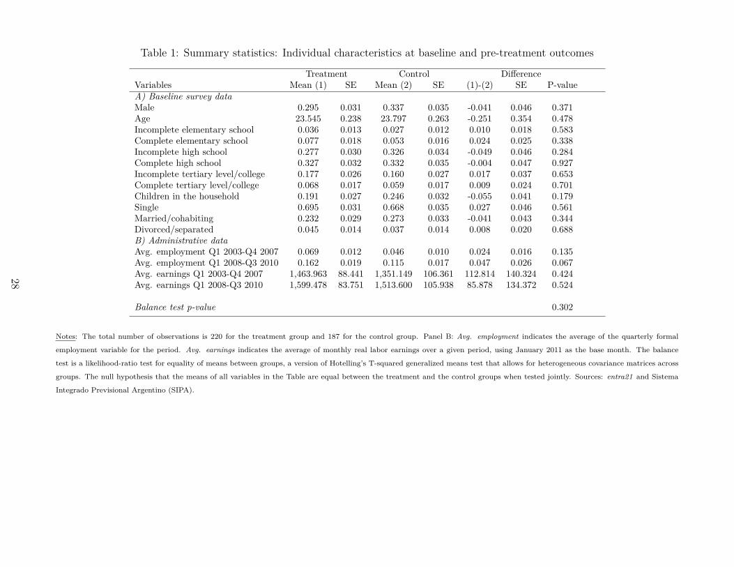
Table 1: Summary statistics: Individual characteristics at baseline and pre-treatment outcomes

Treatment Control DifferenceVariables Mean (1) SE Mean (2) SE (1)-(2) SE P-valueA) Baseline survey dataMale 0.295 0.031 0.337 0.035 -0.041 0.046 0.371Age 23.545 0.238 23.797 0.263 -0.251 0.354 0.478Incomplete elementary school 0.036 0.013 0.027 0.012 0.010 0.018 0.583Complete elementary school 0.077 0.018 0.053 0.016 0.024 0.025 0.338Incomplete high school 0.277 0.030 0.326 0.034 -0.049 0.046 0.284Complete high school 0.327 0.032 0.332 0.035 -0.004 0.047 0.927Incomplete tertiary level/college 0.177 0.026 0.160 0.027 0.017 0.037 0.653Complete tertiary level/college 0.068 0.017 0.059 0.017 0.009 0.024 0.701Children in the household 0.191 0.027 0.246 0.032 -0.055 0.041 0.179Single 0.695 0.031 0.668 0.035 0.027 0.046 0.561Married/cohabiting 0.232 0.029 0.273 0.033 -0.041 0.043 0.344Divorced/separated 0.045 0.014 0.037 0.014 0.008 0.020 0.688B) Administrative dataAvg. employment Q1 2003-Q4 2007 0.069 0.012 0.046 0.010 0.024 0.016 0.135Avg. employment Q1 2008-Q3 2010 0.162 0.019 0.115 0.017 0.047 0.026 0.067Avg. earnings Q1 2003-Q4 2007 1,463.963 88.441 1,351.149 106.361 112.814 140.324 0.424Avg. earnings Q1 2008-Q3 2010 1,599.478 83.751 1,513.600 105.938 85.878 134.372 0.524

Balance test p-value 0.302

Notes: The total number of observations is 220 for the treatment group and 187 for the control group. Panel B: Avg. employment indicates the average of the quarterly formal

employment variable for the period. Avg. earnings indicates the average of monthly real labor earnings over a given period, using January 2011 as the base month. The balance

test is a likelihood-ratio test for equality of means between groups, a version of Hotelling’s T-squared generalized means test that allows for heterogeneous covariance matrices across

groups. The null hypothesis that the means of all variables in the Table are equal between the treatment and the control groups when tested jointly. Sources: entra21 and Sistema

Integrado Previsional Argentino (SIPA).

28

Table 2: Program impact, main results: Intention to treat and treatment on the treated effects

AverageQ2-2011/Q3-2012 Q3-2012 Average

Q4-2012/Q4-2013 Q4-2013 AverageQ1-2014/Q1-2015 Q1-2015

AveragePost

Treatment

PanelANCOVA

A. Formal employmentTreatment group - ITT 0.0796** 0.1020** 0.0434 0.0382 0.0142 0.0171 0.0478 0.0417

[0.0371] [0.0465] [0.0403] [0.0450] [0.0436] [0.0475] [0.0351] [0.0340]Completed training - TOT 0.1641** 0.2104** 0.0895 0.0787 0.0390 0.0352 0.0987 0.0849

[0.0762] [0.0962] [0.0831] [0.0925] [0.0895] [0.0979] [0.0723] [0.0691]Control group mean 0.2504 0.2460 0.3048 0.2888 0.3294 0.3262 0.2921 0.2921B. Monthly earningsTreatment group - ITT 332.23*** 328.18** 179.00 98.96 - - 265.19** 253.53**

[124.77] [149.34] [151.70] [159.27] [127.59] [117.00]Completed training - TOT 691.20*** 664.43** 362.41 200.35 - - 536.91** 517.62**

[243.32] [300.55] [307.27] [322.60] [257.31] [237.87]Control group mean 512.04 623.50 775.47 809.29 627.29 632.80

Observations 407 407 407 407 407 407 407 A 6,512B 4,477

Notes: the TOT coefficients correspond to instrumental variable regressions where the completed training indicator is instrumented by the treatmentassignment (lottery) variable. All regressions include controls for gender, year of birth dummies, children in the household, education level, and maritalstatus. All regressions also include the average of the pre-treatment formal employment variable for the period Q1-2008 to Q3-2010. Regressions in PanelB also include measures of pre-treatment earnings for the same period. Earnings data not available for the Q1-2014/Q1-2015 period. The ANCOVAestimates correspond to panel regressions with time effects for the post-treatment period, including the pre-treatment average as a control (McKenzie,2012). Sources: entra21 and Sistema Integrado Previsional Argentino (SIPA). Robust standard errors in brackets. * significant at 10%; ** significant at5%; *** significant at 1%.

29

Table 3: Effects on formal employment: Heterogeneous impact


Q4-2012/Q4-2013 Q4-2013 AverageQ1-2014/Q1-2015 Q1-2015 Average

Q2-2011/Q1-2015A. By genderTreatment effect: Men 0.2446*** 0.2947*** 0.1992*** 0.2072** 0.1414* 0.1238 0.1982***

[0.0726] [0.0884] [0.0759] [0.0917] [0.0836] [0.0900] [0.0662]T.E. Difference: Women/Men -0.2392*** -0.2793*** -0.2258*** -0.2450** -0.1843* -0.1547 -0.2179***

[0.0822] [0.1010] [0.0870] [0.1026] [0.0953] [0.1038] [0.0748]Women/Men difference (controls) 0.0240 0.0182 0.0927 0.0756 0.0256 0.0538 0.0460

[0.0601] [0.0729] [0.0665] [0.0760] [0.0706] [0.0770] [0.0552]Observations 407 407 407 407 407 407 407Control group mean 0.2137 0.2177 0.2500 0.2500 0.2952 0.2823 0.2505B. Age groups 18-24/25-30Treatment effect: Age 18-24 0.1188** 0.1415** 0.1019* 0.0901 0.0862 0.0943 0.1033**

[0.0507] [0.0632] [0.0549] [0.0621] [0.0590] [0.0652] [0.0473]T.E. Difference: Younger/Older -0.0889 -0.0973 -0.1202 -0.1026 -0.1463* -0.1615* -0.1166*

[0.0709] [0.0873] [0.0792] [0.0878] [0.0840] [0.0909] [0.0675]Younger/Older difference (controls) -0.0351 0.0091 0.0062 0.0318 -0.0219 -0.0017 -0.0181

[0.0547] [0.0690] [0.0621] [0.0692] [0.0664] [0.0717] [0.0526]Observations 407 407 407 407 407 407 407Control group mean 0.2933 0.2692 0.3385 0.3269 0.3635 0.3462 0.3293

Notes: Regression controls as described in the notes to Table 2, with the exception of the regressions in panel B in which the year of birth categorieswere replaced with age range categories. Sources: entra21 , and Sistema Integrado Previsional Argentino (SIPA). Robust standard errors in brackets. *significant at 10%; ** significant at 5%; *** significant at 1%.

30

Table 4: Program effects on monthly earnings: Heterogeneous impact and bounds


Q4-2012/Q4-2013 Q4-2013 AverageQ2-2011/Q4-2013

Panel A. By genderTreatment effect: Men 1,110.67*** 1,268.33*** 983.40*** 758.00** 1,054.99***

[276.17] [328.20] [339.43] [372.37] [280.00]T.E. Difference: Women/Men -1,097.68*** -1,325.70*** -1,134.28*** -929.31** -1,113.69***

[282.44] [343.45] [353.90] [390.18] [288.97]Women/Men difference (controls) -35.97 -54.84 199.69 250.10 67.13

[157.79] [217.41] [217.88] [250.42] [171.19]Observations 407 407 407 407 407Control group mean 442.0882 542.6750 641.6870 666.0570 529.4127Panel B. Age groups 18-24/25-30Treatment effect: Age 18-24 370.51** 400.35** 319.20 206.89 348.06**

[160.52] [198.81] [197.91] [216.19] [167.95]T.E. Difference: Younger/Older -74.30 -168.66 -288.15 -182.15 -167.86

[221.55] [268.71] [267.75] [287.23] [226.94]Younger/Older difference (controls) 52.89 101.52 -11.16 -66.17 24.87

[152.14] [194.04] [192.62] [213.11] [160.20]Observations 407 407 407 407 407Control group mean 578.7615 672.2666 876.1388 976.2771 708.8640Panel C. BoundsLower Bound (monotonicity only) -467.14 -1,084.30 -247.03 -369.44 -24.33Lower Bound (Attanasio et al) 506.16 219.85 427.14 265.00 576.75Upper Bound 1,479.46 1,524.00 1,101.30 899.43 1,177.82

Notes: Regression controls as described in the notes to Table 2, with the exception of the regressions in panel B in which the year of birth categories werereplaced with age range categories. See Section 4 for details about the construction of earning bounds. Sources: entra21 and Sistema Integrado PrevisionalArgentino (SIPA). Robust standard errors in brackets. * significant at 10%; ** significant at 5%; *** significant at 1%.

31

Table 5: Program impact on employment aggregates over time: Ever formally employed, ever enteredand ever left formal employment

Q2-2011/Q3-2012 Q4-2012/Q4-2013 Q1-2014/Q1-2015 Q2-2011/Q1-2015A. Ever formally employedTreatment group 0.1134** 0.0793* 0.0114 0.0805*

[0.0487] [0.0473] [0.0495] [0.0463]Control group mean 0.4011 0.4011 0.4278 0.5829B. Ever entered formal employmentTreatment group 0.0422 0.0043 0.0044 0.0436

[0.0466] [0.0417] [0.0360] [0.0486]Control group mean 0.2727 0.2193 0.1497 0.4866C. Ever left formal employmentTreatment group 0.0069 0.0483 0.0125 0.0540

[0.0440] [0.0409] [0.0370] [0.0499]Control group mean 0.2567 0.1711 0.1551 0.4278Observations 407 407 407 407

Notes: Regression controls as described in the notes to Table 2. Sources: entra21 and Sistema Integrado PrevisionalArgentino (SIPA). Robust standard errors in brackets. * significant at 10%; ** significant at 5%; *** significant at1%.

32

Table 6: Employment transitions (monthly data)

Formal employment04-2011/09-2012




A. Full samplePersistence 0.0346* -0.0165 -0.0062 0.0032

[0.0183] [0.0139] [0.0125] [0.0101]Access 0.0014 0.0079 0.0016 0.0028

[0.0062] [0.0062] [0.0072] [0.0047]Dependence 0.8522*** 0.9170*** 0.9288*** 0.8803***

[0.0176] [0.0118] [0.0116] [0.0088]Observations 7,326 5,698 6,105 19,536B. Women onlyPersistence -0.0139 -0.0362* -0.0265 -0.0236*

[0.0216] [0.0189] [0.0168] [0.0130]Access -0.0007 0.0074 -0.0026 0.0006

[0.0061] [0.0058] [0.0074] [0.0046]Dependence 0.8966*** 0.9354*** 0.9353*** 0.9033***

[0.0191] [0.0127] [0.0134] [0.0103]Observations 5,022 3,906 4,185 13,392C. Men onlyPersistence 0.0996*** 0.0074 0.0189 0.0384**

[0.0291] [0.0219] [0.0201] [0.0158]Access 0.0172 0.0267 0.0191 0.0169

[0.0189] [0.0201] [0.0198] [0.0133]Dependence 0.7690*** 0.8771*** 0.9034*** 0.8357***

[0.0298] [0.0232] [0.0229] [0.0149]Observations 2,304 1,792 1,920 6,144D. Age group 18-24Persistence 0.0560** -0.0029 0.0107 0.0206

[0.0246] [0.0172] [0.0156] [0.0129]Access 0.0042 0.0107 0.0085 0.0066

[0.0096] [0.0094] [0.0107] [0.0070]Dependence 0.8302*** 0.9045*** 0.9175*** 0.8651***

[0.0239] [0.0168] [0.0157] [0.0117]Observations 4,158 3,234 3,465 11,088E. Age group 25-30Persistence -0.0024 -0.0377 -0.0403* -0.0273

[0.0254] [0.0264] [0.0236] [0.0174]Access -0.0011 0.0007 -0.0107 -0.0039

[0.0080] [0.0081] [0.0094] [0.0061]Dependence 0.8856*** 0.9268*** 0.9405*** 0.8998***

[0.0237] [0.0172] [0.0166] [0.0129]Observations 3,168 2,464 2,640 8,448

Notes: Regression controls as described in the notes to Table 2. The estimates correspond to the model in Equation2. The “Persistence” coefficient corresponds to that of the interaction between the treatment group indicator andthe outcome in the previous period, and captures the probability of continuing in employment once the individualis employed. The coefficient for “Access” corresponds to the interaction between the treatment group indicator andthe transformation 1 − Yi,t−1 (which indicates whether individual i was not employed in the previous period), andcaptures the probability of entering employment when the individual is unemployed. The coefficient on “Dependence”captures the overall degree of dependence of the current employment status on that of the previous period forindividuals in both the treatment and the control groups. Sources: entra21 and Sistema Integrado PrevisionalArgentino (SIPA). Standard errors clustered by individuals in brackets. * significant at 10%; ** significant at 5%;*** significant at 1%.

33

Table 7: Probability of staying with the same employer from one year to the following year

Same employerQ3-2010&Q3-2011



A. Full sampleTreatment group -0.0130 0.0413 0.0425

[0.0117] [0.0356] [0.0306]Observations 407 407 407Control group mean 0.0214 0.1176 0.0749B. By genderTreatment effect: Men -0.0185 0.1523** 0.0723

[0.0269] [0.0716] [0.0620]T.E. Difference: Women/Men 0.0086 -0.1608** -0.0433

[0.0304] [0.0813] [0.0699]Women/Men difference (controls) 0.0149 -0.0463 -0.0050

[0.0232] [0.0565] [0.0458]Observations 407 407 407Control group mean 0.0161 0.1210 0.0726C. Age groups 18-24/25-30Treatment effect: Age 18-24 -0.0158 0.0955* 0.0716

[0.0198] [0.0519] [0.0435]T.E. Difference: Younger/Older 0.0025 -0.1209* -0.0587

[0.0237] [0.0676] [0.0587]Younger/Older difference (controls) -0.0145 -0.0028 0.0028

[0.0227] [0.0518] [0.0430]Observations 407 407 407Control group mean 0.0288 0.1346 0.0769

Notes: Regression controls as described in the notes to Table 2 with the exception of the regressions in panel C inwhich the year of birth categories were replaced with age range categories. Sources: entra21 and Sistema IntegradoPrevisional Argentino (SIPA). Robust standard errors in brackets. * significant at 10%; ** significant at 5%; ***significant at 1%.

34

Figure 1: Evolution of formal employment and labor earnings for the treatment and the control groups

A. Formal employment by group, quarterly

00.

100.

200.

300.

40

Q1−08

Q2−08

Q3−08

Q4−08

Q1−09

Q2−09

Q3−09

Q4−09

Q1−10

Q2−10

Q3−10

Q4−10

Q1−11

Q2−11

Q3−11

Q4−11

Q1−12

Q2−12

Q3−12

Q4−12

Q1−13

Q2−13

Q3−13

Q4−13

Q1−14

Q2−14

Q3−14

Q4−14

Q1−15

Quarter

Treatment Control

B. Average real labor earnings by group, quarterly

020

040

060

080

010

0012

00

Q1−08

Q2−08

Q3−08

Q4−08

Q1−09

Q2−09

Q3−09

Q4−09

Q1−10

Q2−10

Q3−10

Q4−10

Q1−11

Q2−11

Q3−11

Q4−11

Q1−12

Q2−12

Q3−12

Q4−12

Q1−13

Q2−13

Q3−13

Q4−13

Quarter

Treatment Control

Notes: The vertical line indicates when the program took place. Sources: entra21 and Sistema IntegradoPrevisional Argentino (SIPA).

35

Appendix B: Main results without controls

Table F.1: Program impact, intention to treat and treatment on the treated. No control variables


Q4-2012/Q4-2013 Q4-2013 AverageQ1-2014/Q1-2015 Q1-2015 Average All

Post-TreatA. Formal employmentTreatment group - ITT 0.0867** 0.0949** 0.0479 0.0430 0.0188 0.0193 0.0533

[0.0383] [0.0450] [0.0417] [0.0460] [0.0431] [0.0471] [0.0361]Completed training - TOT 0.1799** 0.1970** 0.0994 0.0893 0.0390 0.0400 0.1107

[0.0795] [0.0935] [0.0864] [0.0953] [0.0895] [0.0977] [0.0749]Control group mean 0.2504 0.2460 0.3048 0.2888 0.3294 0.3262 0.2921B. Monthly earningsTreatment group - ITT 333.03*** 322.44** 254.12* 203.65 298.51**

[117.86] [140.71] [147.66] [160.13] [123.16]Completed training - TOT 691.20*** 669.22** 527.42* 422.68 - 619.55**

[243.32] [289.85] [307.13] [333.23] [255.39]Control group mean 512.04 623.50 775.47 809.29 - - 627.29Observations 407 407 407 407 407 407 407

Notes: the TOT coefficients correspond to instrumental variable regressions where the completed training indicator is instrumented by the treatmentassignment (lottery) variable. The regressions do not include any control variables. Earnings data not available for the Q1-2014/Q1-2015 period. Sources:entra21 and Sistema Integrado Previsional Argentino (SIPA). Robust standard errors in brackets. * significant at 10%; ** significant at 5%; *** significantat 1%.

i

Long Run Effects of Youth Training Programs: Experimental ...ftp.iza.org/dp9784.pdf · IZA...

Documents

Transcript of Long Run Effects of Youth Training Programs: Experimental ...ftp.iza.org/dp9784.pdf · IZA...