Long-Run and Short-Run Co-Movements between Oil and Agricultural Futures Prices

By

Robert J. Myers, Stanley R. Johnson, Michael Helmar and Harry Baumes*

July, 2015

Abstract: The relationship between oil prices and the prices of agricultural feedstocks for biofuel has received considerable attention in the recent literature. Here we extend the recent common trend-common cycle analysis of Myers et al. (2014), which investigated long-run and short-run co-movements between fuel and agricultural spot prices, to the case of futures prices. It is often argued that the speculative nature of futures trading leads to excess co-movement between different futures price series. Our results do not support this hypothesis and show there is even less co-movement between futures prices for oil and agricultural biofuel feedstocks than there is between spot prices for these same commodities. This suggests variations in agricultural futures prices are dominated by factors not related to changes in oil prices, such as agricultural supply response and the non-biofuel demand for feedstocks.

* Respectively, University Distinguished Professor, Michigan State University, East Lansing MI 48824; Board Chair, National Center for Food and Agricultural Policy, Washington, DC 20036; Research Scientist, University of Nevada, Reno, Reno Nevada 89557; and Director, Office of Energy Policy and New Uses/Office of the Chief Economist/USDA. Washington DC 20250-3815. Research supported by USDA Cooperative Agreement.

1

Long-Run and Short-Run Co-Movements between Oil and Agricultural Futures Prices

Introduction

The relationship between prices for fuels (crude-oil, gasoline, and ethanol) and

agricultural feedstocks for biofuel (particularly corn and soybeans) has become an important

economic and policy issue. There is now considerable evidence that the growth in biofuel

production has increased the demand for, and price of, agricultural feedstocks—but the evidence

on the extent to which changes in fuel prices get transmitted to agricultural feedstock prices is

more mixed (Zilberman et al., 2013). This is important because if there is strong price

transmission then higher (lower) fuel prices can be expected to lead to higher (lower) food

prices, changing the incentives for agricultural production and putting pressure on the food

security of low income households (Runge and Senauer, 2007; Mitchell, 2008). However, if

variations in fuel prices do not transmit readily to agricultural prices then many of these concerns

are misplaced and oil price shocks can be expected to have much smaller and more short-lived

effects on agricultural and food prices.

A recent study by Myers et al. (2014) investigates long-run and short-run co-movement

between spot prices for crude oil, gasoline, and ethanol and spot prices of corn and soybeans.

Results suggest that spot fuel prices transmit to spot agricultural feedstock prices in the short run,

but that the relationship dissipates in the long run. In particular, long-run equilibrium spot fuel

and spot agricultural prices were found to be driven by separate stochastic trends and therefore

“meander away” from one another over long time horizons. Furthermore, shocks to long-run

equilibrium spot fuel prices only explain a relatively small portion of the forecast error variance

in long-run equilibrium spot agricultural prices. These results suggest that while spot fuel and

spot agricultural prices co-move to some extent over intermediate time horizons, in the long run

2

spot agricultural prices are determined primarily by agricultural supply conditions (e.g.,

productivity growth, acreage expansion etc.) and the non-biofuel demand for agricultural

feedstocks (e.g., the derived demand for livestock feed as incomes grow), with fuel prices

playing a relatively minor role in long-run agricultural spot price determination.

An interesting additional question is whether similar kinds of relationships exist between

futures prices for fuels and futures prices for biofuel feedstocks. Futures prices differ from spot

prices because they reflect the aggregated expectations of market participants regarding the

future value of the underlying commodity at the maturity date specified on the futures contract.

A futures contract is therefore a different asset than the underlying physical commodity, even

when quality specifications and delivery location are the same. Furthermore, participation in

futures trading does not require production, consumption, or ownership of the physical

commodity and so opens up additional opportunities for low-cost speculative trading activity.

Some have argued that this additional speculative activity can have an important influence on

futures price determination, leading to futures prices that co-move in excess of co-movement in

the spot prices of the underlying physical commodities (e.g., Juvenal and Petrella, 2011).

This paper builds on Myers et al. (2014) by investigating long-run and short-run co-

movements between futures prices for crude oil and futures prices for biofuel feedstocks,

specifically corn and soybeans. We do not include gasoline prices in the analysis because Myers

et al. (2014) show that gasoline and crude oil prices co-move strongly in both the short-run and

long-run. We also do not include ethanol futures prices in the analysis because ethanol futures

only began trading in 2005, which would limit the length of time series data available for

analysis. Finally, Myers et al. (2014) include exchange rates in their spot price analysis to

account for the possibility that exchange rates provide an important link between energy and

agricultural prices, both of which are traded goods. In the futures price analysis reported here,

3

however, we do not include exchange rates because Myers et al. (2014) found that including the

exchange rate explicitly did not have a significant influence on inferences regarding price

transmission between fuel and biofuel feedstock prices. We also investigated including other

potential biofuel feedstock prices (e.g., wheat, soybean oil, other oil seeds, etc.) in the futures

price analysis but found results followed an almost identical pattern to those using corn and

soybean prices only (see Myers et. al, 2012 for details). For all of these reasons we focus here on

co-movements between just three futures prices (crude oil, corn, and soybeans).

It is important to investigate futures price as well as spot price co-movement between fuel

and agricultural biofuel feedstocks because of the potentially different market participants and

price relationships that can occur in futures versus spot commodity markets. The contribution of

the current paper is that it investigates long-run and short-run relationships between futures

prices for oil and biofuel feedstock prices, and compares these results to those from the previous

spot price analysis. Results lead to some new insights into the influence of futures market trading

on commodity price co-movements, and on the relationship between oil and agricultural

commodity prices.

Empirical Approach

To characterize the relationships among a set of n different fuel and agricultural futures

prices, let tp be an (nx1) vector of the logarithms of each commodity futures price.1 Because

each futures contract has a fixed maturity date, a time series of futures prices will have jumps in

time to maturity as the series switches from one futures contract to the next as the maturity date

1 Log transformations are commonly used in commodity price modeling because they are consistent with the statistical properties of most price data and facilitate interpretation of coefficients in terms of proportional relationships between prices.

4

for the first contract expires. This feature will be taken into account in the empirical analysis

which follows.

We follow the empirical approach in Myers et al. (2014). The first step is to decompose

each (log) price into a permanent component tτ and a transitory or cyclical component tη such

that:

(1) ttt ητp += .

The permanent component is defined as [ ]∑=

+∞→∆−∆+=

s

kttkt

stt E

1| )(ˆlim pppτ where tkt |ˆ +∆p is the

kth step ahead best linear unbiased forecast of tp∆ conditional on information available at time t.

By definition, tτ is a vector of prices expected in the very long-run (i.e., as the forecast horizon

goes to infinity) conditional on information available at time t but adjusted back to time t by

subtracting any known trend or drift. Futures prices should be nonstationary based on no-

arbitrage arguments and there is considerable existing evidence to support this hypothesis. In this

case it can be shown that tτ follows a pure random walk (possibly with drift) and is therefore

itself nonstationary (see Beveridge and Nelson, 1981 and Stock and Watson, 1988). Because tτ

is the current value of the price that is consistent with expected full adjustment over an infinite

time-horizon we call it the “long-run equilibrium value” of the series. By definition, tη is then

stationary and represents transitory deviations around long-run equilibrium values.

Because the components of tτ are nonstationary they may also be cointegrated. Suppose

all prices are nonstationary and there are nr < cointegration relationships among the n prices in

the system. Then tτ can be expressed in terms of a smaller number rnk −= of “common

trends” so that the long-run equilibrium prices can be written as tt τAτ ~= where tτ~ is a (k x 1)

5

vector of common trends (random walks) and A is an (n x k) loading matrix that has full column

rank (Hecq, Palm and Urbain, 2000).

Similarly, Vahid and Engle (1993) have shown that the cyclical part of the series may

also have common components. In particular, assuming all prices are nonstationary then tp∆ is

said to be co-dependent with common serial correlation features (hereafter just “co-dependent”)

if there are c < n linear combinations of tp∆ that are innovations with respect to information

available at time t – 1 (i.e., linear combinations of tp∆ that are not serially correlated). These

linear combinations are called “co-feature vectors” and they imply that the cyclical component

can be written as tt ηBη ~= where tη~ is an (l x 1) vector of common cyclical components with l

= n – c, and B is an (n x l) loading matrix for the common cycles that has full column rank (see

Vahid and Engle, 1993).

Allowing for both cointegration and co-dependency the decomposition (1) can be

expressed:

(2) ttt ηBτAp ~~ += .

If there is no cointegration or co-dependency then tτ~ and tη

~ will be of full dimension n.

However, when cointegration and/or co-dependency exist imposing the common trend and

common cycle restrictions in (2) will help identify the nature of long-run and short-run

relationships between the prices in the system.

Measures of Long-Run and Short-Run Co-Movement

Myers et al. (2014) suggest measuring the extent of long-run co-movement between two

prices itp and jtp by the size of the correlation coefficient between the innovations in their

6

permanent component, ),( jtitCorr ττ ∆∆ . If the long-run equilibrium values of the prices move

closely together this correlation will be close to one, while if movements in the long-run

equilibrium prices are completely unrelated this correlation will be zero. The correlation between

the innovations in the permanent components therefore has a natural interpretation as a measure

of long-run co-movement between prices.

The number of common trends k in tτ~ influences long-run co-movement between prices.

For example, suppose that itp and jtp are both driven by a single common trend (i.e., they are

cointegrated). Then the equilibrium values of both prices would move together perfectly and

1),( =∆∆ jtitCorr ττ . In this case the long-run equilibrium prices maintain a fixed relationship

with one another and there is “perfect long-run co-movement” between the prices. Alternatively,

if the two prices are not driven by a common trend (i.e., are not cointegrated) then

1),( <∆∆ jtitCorr ττ and the two prices will be unrelated in the very long-run (infinite horizon

forecasts of any linear combination of the prices will have infinite variance). In the limiting case

when the permanent components of the two prices are separate uncorrelated random walks then

the long-run equilibrium values of the prices move completely independently and

0),( =∆∆ jtitCorr ττ . In this case there is “no long-run co-movement” in the prices. Intermediate

outcomes 1),(0 <∆∆< jtitCorr ττ indicate long-run equilibrium values of prices move together

over intermediate time intervals because innovations in their permanent component are

correlated, even though these prices would eventually meander apart and become unrelated in the

long-run. In this case there is “intermediate-run co-movement” and values of ),( jtitCorr ττ ∆∆

close to one indicate stronger intermediate-run co-movement while values close to zero indicate

weaker intermediate run co-movement.

7

Myers et al. (2014) suggest measuring short-run co-movement between any two prices

itp and jtp by the unconditional correlation between their transitory components, ),( jtitCorr ηη .

Because the transitory components are stationary this unconditional correlation is well-defined

and provides a convenient summary measure of the extent to which prices co-move in the short

run as they converge back to long-run equilibrium values. Just as the number of common trends

k influence the extent of co-movement between long-run equilibrium prices, the number of

common cycles l in tη~ influences the extent of co-movement between the transitory

components. For example, suppose that itp∆ and jtp∆ are both driven by a single common cycle

(i.e., they are co-dependent). Then their transitory components would move together perfectly,

and 1),( =jtitCorr ηη . In this case there is “perfect short-run co-movement” between the prices.

Alternatively, if the two prices are not co-dependent then each price is driven by separate

cyclical components, and 1),( <jtitCorr ηη . In the limiting case of no relationship between the

transitory components then 0),( =jtitCorr ηη and there is “no short-run co-movement” between

the series. In the intermediate case of 1),(0 << jtitCorr ηη values close to one indicate stronger

co-movement in adjustments towards long-run equilibrium while values close to zero indicate

weaker short-run co-movement.

Together, the estimated correlation matrices of tτ∆ and tη provide detailed information

on the ways in which the prices are related to one another over different forecast horizons.

8

Estimation and Testing

Estimation and testing for nonstationarity and cointegration are now standard and will not

be detailed here.3 Estimation and testing for co-dependence is outlined in Vahid and Engle

(1993) and their procedures are adapted to the current case of fuel and agricultural feedstock

prices in Myers et al. (2014). We do not detail the co-dependency testing procedures again here

but note that estimation and testing is conditional on cointegration restrictions and so based on a

vector error correction (VEC) representation:

(3) ∑=

−− +∆++=∆q

itititt

11 εpΓαzμp

where tt pβz '= is the (r x 1) vector of equilibrium errors from the r cointegrating relationships

and β contains the cointegrating vectors. Testing for co-dependence is based on the canonical

correlations between tp∆ and },...,,{ 11 qtttt −−− ∆∆= ppzw as outlined in Myers et al. (2014). If

co-dependence is found the co-feature vectors form a (n x c) matrix β~

such that each element of

tpβ ∆′~ is an innovation with respect to the information set tw . Once the number of cofeature

vectors has been established via testing we estimate β~

by imposing the co-dependency

restrictions on the VEC model (3) and estimating the resulting “pseudo-structural form” using

maximum likelihood. The appropriate pseudo-structural form is derived by first noting that β~

is

not unique and so can be normalized to:

(4)

=

×−*

)(

~~

ccn

c

β

Iβ

for a set of unknown parameters*~β . Then the co-dependency restrictions imply (up to a constant

term) the following restrictions on the VEC model (3):

3 More details are available in Hamilton (1994) and many other econometric texts.

9

(5) t

q

iit

i

nct

rct

cnccn

cεp

Γ

0z

α

0p

I0

βI+∆

+

=∆

∑

=−

×−

×

−×− 1*

)(1*

)(

)(

* '~

where the * differentiates parameters from their unrestricted counterparts, *α is rcn ×− )( , and

the *iΓ are ncn ×− )( . Equation (5) can then be estimated using maximum likelihood and

imposes the following restrictions on the VEC model (3):

(6)

= ×

−

−×−*

)(

1

)(

* '~

α

0

I0

βIα

rc

cnccn

c and

= ×

−

−×−*

)(

1

)(

* '~

i

nc

cnccn

ci

Γ

0

I0

βIΓ for i = 1, 2, …q.

These restrictions will be useful for computing the permanent-transitory decomposition under

co-dependency restrictions.

Computing the Decomposition

Once the parameters of the model have been estimated, either with or without

cointegration and co-dependency restrictions as indicated by test results, decomposing each price

into permanent and transitory components is straightforward as shown in Myers et al. (2014). In

particular, the decomposition for the VEC representation (3) can be computed as:

(7a) tnt L pΓαβΓPIτ )(]')1()[( 1−−−=

(7b) ttnt L PppΨαβΓPIη +∆−−−= − )(]')1()[( 1

where qqn LLL ΓΓIΓ −−−= ...)( 1 , qn ΓΓIΓ −−−= ...)1( 1 ,

1110 ...)( −

−+++= qq LLL ΨΨΨΨ with ∑

+=

=q

jiij

1

ΓΨ , and where

'}]')1(['{]')1([ 111 βααβΓβααβΓP −−− −−= .

These formulas already impose cointegration restrictions directly, so decompositions computed

using (7) will satisfy all appropriate cointegration restrictions. If there is no cointegration (r = 0)

10

these formulas are still applicable if we set 0αβ =' and P = 0. If short-run co-dependency

behavior is found then the decomposition (7) is still applicable, except that values for α and the

iΓ must satisfy the restrictions in (6) with *~β , *

α , and *iΓ estimated using the pseudo-structural

form (5). Imposing these restrictions ensures that the transitory component tη computed from

(7b) exhibits all of the behavior implied by the co-dependency restrictions.

Evaluating Potential Nonlinearities and Regime Shifts

As argued by Myers et al. (2014), it is possible that co-movement in commodity prices

involves nonlinearities that are not well captured by the linear cointegration and co-dependency

models discussed so far. For example it could be that the price relationships experienced a

structural change due to the growth of biofuels, or that when production of biofuel reaches

certain threshold levels then the nature of the price relationships change. One way to model such

nonlinearities is to allow model parameters to change over different ranges of values for

underlying threshold variables, such as biofuel production levels, commodity stock levels, and

time.

To allow for such regime changes, suppose the estimation equations for the multivariate

price model take the general form ttt εθwfp +=∆ );( where tw is as defined previously and θ

an associated parameter vector. Then we can define a multiple threshold model as:

(8) tjtt εθwfp +=∆ );( )(δx jt R∈

where j indexes a set of multiple regimes defined by values of the exogenous threshold variable

vector tx lying in a set of nonintersecting and exhaustive sets )(δjR defined by the parameter

vector δ . After identifying and estimating the separate models for each regime, the

cointegration, co-dependency and permanent-transitory decomposition analyses can then be

11

applied regime by regime to isolate the extent of long-run and short-run co-movement in

different regimes (see Myers and Jayne, 2012).

Given the well-known difficulties of testing formally for threshold effects (see Davies,

1987; Hansen, 1996; and Balagtas and Holt, 2008) we follow Myers et al. (2014) and use the

Gonzalo and Pitarakis (2002) BIC-like criterion function:

(10) [ ]

−−= md

T

TLL

TmQ TTT

)ln()(

2max)( δδ

to evaluate the existence of threshold nonlinearities. Here TL is the log-likelihood value for the

single regime (no threshold) model, )(δTL is the full sample log-likelihood value for the multi-

regime model with thresholds δ , d is the number of parameters to be estimated in the single

regime model, and m is the number of threshold parameters. The criterion is based on a

likelihood ratio statistic but imposes a penalty for over-parameterization that is similar to the BIC

criterion for evaluating lag length. Threshold and regime selection is then based on:

(11) )(maxargˆ0

mQm TMm≤≤

=

where M is the maximum number of thresholds to be considered. Gonzalo and Pitarakis provide

simulation evidence to suggest this criterion performs well in selecting the appropriate number of

thresholds and regimes.

Data and Preliminary Analysis

The application uses end-of-month current and one-month lags of the prices for the

nearest maturing futures contract for CBOT corn, soybeans, and West Texas Intermediate (WTI)

crude oil (hereafter “oil”) traded on NYMEX. The one-period lags are used to construct a series

of futures price differences that always have the same maturity date (i.e., futures price “changes”

12

are always computed using the same underlying futures contract, not from the difference in

prices between two contracts with different maturity dates). The sample period is January 1990

through August 2012.

Table 1 shows the nearby contract expiration months for each month of the year. In the

corn futures market there are five contracts for delivery in March, May, July, September, and

December. For soybeans there are seven contracts for delivery in January, March, May, July,

August, September, and November. There are oil futures contracts for every month so the nearby

futures price data are always taken from a contract expiring in the subsequent month. Using this

approach recorded price changes are always changes in futures prices for contracts for the same

maturity date, which avoids introducing spurious variation in futures price change data that are

due only to changes in time to maturity.

To give some initial insights into the data we plot nearby futures prices for oil, corn, and

soybeans over the sample period, each normalized to a value of one in January 1990 (see figure

1). As can be immediately observed, nearby futures prices for corn and soybeans move closely

together over the entire sample period. Nearby oil futures prices appear to co-move with the

agricultural futures during some periods, but also go through periods where there is little

observed co-movement. This suggests a detailed investigation into the extent and nature of co-

movement between these series should provide some interesting insights.

Model Estimation and Testing Results

Because of the considerable existing evidence that commodity futures prices are

nonstationary, and because stationary futures prices would imply the existence of systematic

profitable futures trading strategies, we do not report detailed tests for nonstationarity. However,

13

augmented Dickey-Fuller and Phillips-Perron tests strongly support nonstationarity of all three

nearby futures price series.

Given nonstationarity it is important to test for cointegration because this will impose

restrictions on the permanent-temporary decomposition. We undertook both Engle-Granger and

Johansen trace tests for cointegration. The results are reported in Table 2 and show strong

evidence of a single cointegration relationship between nearby corn and soybean futures prices,

but no cointegration between the nearby futures price for oil and either of the agricultural futures

prices. These findings are similar to those found for spot oil and agricultural prices in Myers et

al. (2014).

We also need to estimate the cointegrating vector. Results from both least squares

regression, and Johansen’s VEC maximum likelihood method for estimating the cointegrating

vector, are reported in table 3. Both estimates suggest strongly that the cointegrating vector is (1,

-1), with the Johansen procedure (which provides consistent standard errors) showing a very

tight confidence interval around this value. Remembering that the prices are in logarithms, this

shows that nearby corn and soybean futures prices remain proportional to one another in the

long-run. This result is consistent with economic intuition and we impose the long-run

proportionality (cointegration) constraint from here on.

The next step is to test for co-dependency. The canonical correlation statistics for testing

at least one and then at least two co-dependency relationships, along with their associated p-

values, are shown in table 4. The result suggests two co-dependency relationships which implies

one common transitory component is driving all of the price series.

Estimating the resulting pseudo-structural form with one cointegration and two co-

dependency restrictions imposed revealed that the agricultural price differences could be

excluded from the oil co-dependency relationship (likelihood ratio p-value = 0.985). This

14

suggests that changes in nearby futures prices for oil are already innovations with respect to the

information set },...,,{ 11 qtttt −−− ∆∆= ppzw . In other words, oil futures prices follow a pure

random walk with all price movement due the permanent component (the series has no transitory

component). This is exactly what we would expect for futures prices generated from a well-

functioning futures market because it means futures price changes are unpredictable based on

past information, without even short-run temporary predictable cycles. On the other hand, corn

and soybean futures are found to have small transitory components that suggest at least some

predictability of short-run cyclical price movements. However, the majority of the price variation

still comes from the (unpredictable) permanent component of these series so predictability of

price changes remains low and short-run.

Full results for the restricted pseudo structural form estimated via maximum likelihood

are provided in table 5. The first two equations for oil and corn are the two co-dependency

relationships, showing that oil price changes are pure innovations and a linear combination of

corn and soybean futures price changes, given by )68701()1( .,~

, *SOY −=− β are also innovations

with respect to the defined information set. The third equation (for soybeans) is an error-

correction equation using the difference in log corn and soybean futures prices as the lagged

equilibrium error term (i.e. imposing long-run proportionality between corn and soybean futures

prices as the cointegration restriction). This specification is supported by previous testing results

but we note that the results suggest very little ability to forecast futures price changes (see the

very low 2R in the soybean equation). The pseudo-structural form estimates are of little interest

by themselves and are only shown for completeness and to provide additional insight into the

structure of the empirical model. The main use of the estimates in the current application comes

in operationalizing the permanent-transitory decomposition.

15

Decomposition and Co-Movement Results

The pseudo-structural form estimates are used decompose the three nearby futures price

series into permanent (long-run equilibrium) and transitory (short-run stationary) components

using the decomposition defined in equation (7). Test results showed that the oil futures prices

have no transitory component (all price movements represent permanent changes). However, the

corn and soybean futures process have both permanent and transitory components. The

correlation matrix for changes in the permanent components of each series is shown in table 6.

The corn and soybean futures prices are cointegrated and therefore driven by the same common

trend. Therefore, as expected, the permanent components of the corn and soybean futures are

perfectly correlated, showing perfect long-run co-movement. The oil futures are driven by a

separate trend (not cointegrated with corn and soybean futures) but it is still possible that the two

trends are correlated, showing that the oil and agricultural futures prices move together over

intermediate time horizons. However, table 6 shows that the correlation coefficient between

innovations in the two permanent components is only 0.01, indicating very weak long-run co-

movement between oil futures prices and either corn or soybean futures prices.

Following Myers et al. (2014), we investigate this issue further by computing the

(horizon independent) forecast error variance decomposition from a bivariate model of long-run

equilibrium oil and corn prices. Results show that less than 1% of the variation in the innovations

in the permanent component of corn futures prices is accounted for by variation in the

innovations in the permanent component of oil futures prices. This result continues to hold if we

use corn futures price changes themselves, instead of changes in the permanent component of the

corn futures changes, to do the decomposition. The finding of very weak co-movement between

long-run equilibrium oil and agricultural futures prices is therefore robust to model specification.

16

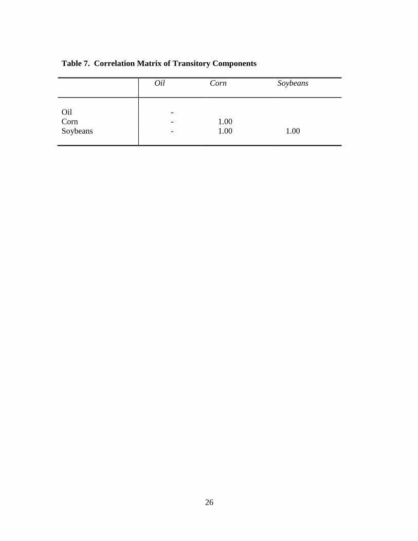
Turning to short-run co-movements, table 7 shows the estimated correlation matrix of

transitory deviations around long-run equilibrium values for the three series. The oil futures

prices have no transitory component and the corn and soybean futures prices are driven by the

same common cycle. Therefore, table 7 shows no results for oil and that the transitory

components of the corn and soybean futures prices are perfectly correlated (as expected). The

results show perfect short-run co-movement between corn and soybean futures prices, but no

short-run co-movement between oil futures and futures prices for the agricultural commodities. It

might seem odd that the corn and soybean series co-move perfectly in both the short run and the

long run, but the prices themselves are not perfectly correlated (though they are clearly highly

correlated). This happens because, although the two prices are driven by the same common trend

and same cyclical component, the prices themselves are different linear combinations of these

two components, and therefore do not need to be perfectly correlated.

Overall the evidence supports strong co-movement between corn and soybean futures

prices in both the long run and the short run. On the other hand, oil futures only co-move very

weakly with the permanent component of corn and soybean futures prices and have no transitory

component. Therefore there is very little co-movement between oil futures prices and either of

the agricultural futures prices in either the long run or the short run.

These results suggest that fluctuations in agricultural futures prices are dominated by

factors related to agricultural supply and the non-energy demand for biofuel feedstocks and are

little influenced by oil futures price movements in either the long run or the short run. The results

are similar to, but even stronger than, the co-movement results found for spot oil, corn, and

soybean prices in Myers et al. (2014). For spot prices, the permanent components of oil and

corn/soybean prices are more correlated (0.49 versus 0.01 found here for futures prices) and the

forecast error variance decomposition of the innovations showed a larger proportion of the

17

variance in the permanent component of spot corn price is due to the permanent component of

spot oil prices (24% versus less than 1% found here for futures prices). Evidently, the nature of

futures price determination leads to even less co-movement between oil and agricultural prices

over any length of run than is found in spot prices. The implication is that there is nothing about

the speculative nature of futures markets, or the ease of participation in futures trading for those

not involved in production or trade of the physical commodities, that leads to more co-movement

between oil and agricultural prices. In fact, the reverse is true with even less co-movement than

in the case of spot prices.

Nonlinearities and Regime Shifts

We evaluated the possibility of nonlinearities using time as the threshold variable and the

Gonzalo-Pitarakis criterion function approach described above. There is some evidence of a

regime shift in the model parameters (i.e., structural change) in March 2003 (GP criterion =

0.125). However, the GP criterion is only slightly greater than zero, indicating the evidence of

structural change is weak. Furthermore, undertaking separate model estimation, decomposition

and co-movement analysis for the two regimes before and after the structural break leads to the

same conclusions as the full sample analysis—strong long-run and short-run co-movement

between corn and soybean futures prices but very weak co-movement between oil futures and

either of the agricultural prices. Therefore we only report complete results for the full sample

analysis.

Conclusions

Common trend-common cycle decompositions were used to evaluate long-run and short-

run co-movement among futures prices for oil, corn, and soybeans. Cointegration tests supported

18

the hypothesis that corn and soybean futures prices are cointegrated and therefore driven by a

single common trend, but oil futures prices are not cointegrated with the agricultural prices and

follow their own long-run trend. Co-dependency tests suggested that oil futures price changes are

uncorrelated with past futures price information and so have no transitory component. However,

corn and soybean futures prices were found to have small transitory components that are driven

by the same common cycle.

The pseudo-structural form was estimated under these cointegration and co-dependency

restrictions and results used to decompose each of the series into permanent and transitory

components. Correlation analysis of the two components across different commodities revealed

that corn and soybean futures prices co-move strongly in both the long run and the short run.

However, oil futures prices have only very weak co-movement with the agricultural futures

prices over any time horizon.

These results are similar to but stronger than the results found for oil, corn, and soybean

spot prices in Myers et al. (2014). Evidently there is even less co-movement between futures

prices for oil and agricultural feedstocks than there is between spot prices for the same

commodities. This is an important result because it is often argued that the speculative nature of

futures trading can generate price movements that go beyond those that can be supported based

on supply and demand fundamentals, and in this sense may lead to excess co-movement between

futures price series. Our results are not consistent with this hypothesis. Instead, our results

indicate that variation in agricultural futures prices are dominated by factors not related to

changes in oil prices, factors such as agricultural supply response and the non-biofuel demand

for feedstocks. One implication of these results is that in the long run we can expect oil and

agricultural futures prices to “meander apart” and be determined by largely separate economic

fundamentals. This suggests that, taking a long-run view, concerns about commodity futures

19

speculation and higher oil futures prices leading to food shortages and agricultural commodity

price booms may have been over-emphasized. Our results suggest that, in the long run, corn and

soybean prices will be driven more by factors such as productivity growth, acreage response, and

the non-ethanol demand for biofuel feedstocks, rather than by changes in oil prices. This does

not imply that increased ethanol production has not had an influence on corn prices. But it does

imply that changes in oil futures prices do not readily transmit to agricultural futures prices in

either the short run or the long run. Our findings are also important because they suggest that

futures trading has no adverse effects in terms of generating more co-movement in oil and

agricultural futures prices than can be supported by co-movement in the underlying spot prices.

20

References

Balagtas, J.V., and M.T. Holt (2008). “The Commodity Terms of Trade, Unit Roots, and

Nonlinear Alternatives: A Smooth Transition Approach.” American Journal of Agricultural Economics 91:87-105.

Beveridge, S. and C.R. Nelson (1981). “A New Approach to Decomposition of Economic Time Series into Permanent and Transitory Components with Particular Attention to Measurement of the Business Cycle.” Journal of Monetary Economics 7: 151-174.

Davies, R.B. (1987). “Hypothesis Testing when a Nuisance Parameter is Present only Under the

Alternative.” Biometrika 74: 33-43. Gonzalo, J., and J.-Y. Pitarakis (2002). “Estimation and Model Selection Based Inference in

Single and Multiple Threshold Models.” Journal of Econometrics 110:319 – 352. Hamilton, J.D. (1994). Time Series Analysis. Princeton University Press, Princeton. Hansen, B.E. (1996). “Inference When a Nuisance Parameter is Not Identified Under the Null

Hypothesis.” Econometrica 64:413-430. Hecq, A., F.C. Palm, and J-P Urbain (2000). “Permanent-Transitory Decomposition in VAR

Models with Cointegration and Common Cycles.” Oxford Bulletin of Economics and Statistics 62(4): 511-532.

Juvenal, L. and I. Petrella (2011). Speculation in the Oil Market. Tech. rep., Research Division,

Federal Reserve Bank of St. Louis, St. Louis, MO.

Mitchell, D. (2008). “A Note on Rising Food Prices.” Policy Research Working Paper 4682, The World Bank, Washington, DC.

Myers, R.J., and T.S. Jayne (2012). “Price Transmission under Multiple Regimes and Thresholds

with an Application to Maize Markets in Southern Africa.” American Journal of Agricultural Economics 94(1): 174-188.

Myers, R.J., S.R. Johnson, M. Helmar, and H. Baumes (2012) “Coherency of Agricultural

Feedstock and Petroleum Prices: An Analysis of Monthly Prices, January 1989 through November 2010” Technical Report to USDA OCE http://www.ncfap.org/documents/CoherencyTechnicalReport.pdf

Myers, R.J., S.R. Johnson, M. Helmar and H. Baumes (2014). “Long-Run and Short-Run Co-

Movements in Energy Prices and the Prices of Agricultural Feedstocks for Biofuel.” American Journal of Agricultural Economics 96(4): 991-1008.

21

Runge, C.F. and B. Senauer (2007). “How Biofuels Could Starve the Poor.” Foreign Affairs May/June.

Stock, J.H. and M.W. Watson (1988). “Testing for Common Trends.” Journal of the American

Statistical Association 83: 1097-1107. Vahid, F. and R.F. Engle (1993). “Common Trends and Common Cycles.” Journal of Applied

Econometrics 8: 341-360. Zilberman, D., G. Hochman, D. Rajagopal, S. Sexton, and G. Timilsina (2013). “The Impact of

Biofuels on Commodity Food Prices: Assessment of Findings.” American Journal of Agricultural Economics 95(2): 275-281.

22

02

46

Nor

mal

ized

Pric

e

1990m1 1995m1 2000m1 2005m1 2010m1Date

Crude Oil Soybeans

Corn

Figure 1. Normalized Monthly Oil, Corn, and Soybean Futures (log) Prices

Table 1. Nearby Futures Contract by Last Day of Month

Actual Month Nearby Contract Month

Corn Soybeans WTI Crude Oil January March Year t March Year t February Year t February March Year t March Year t March Year t March May Year t May Year t April Year t April May Year t May Year t May Year t May July Year t July Year t June Year t June July Year t July Year t July Year t July September Year t August Year t August Year t August September Year t September Year t September Year t September December Year t November Year t October Year t October December Year t November Year t November Year t November December Year t January Year t+1 December Year t December March Year t+1 January Year t+1 January Year t+1

Source: Barchart.com

23

Table 2. Cointegration Test Results Cointegrating Relationship

Engle Granger Statistic

5% Critical Value

Maximum No. of Cointegrating Relationships

Trace Statistic

5% Critical Value

Corn-Oil -2.802 -3.359 0* 10.505 15.41 1 0.495 3.76 Soybeans-Oil -2.586 -3.359 0* 8.665 15.41 1 0.526 3.76 Corn-Soybeans -4.392 -3.359 0 20.638 15.41 1* 0.866 3.76 Corn-Soybeans-Oil -4.391 -3.772 0 29.808 29.68 1* 9.265 15.41 2 0.424 3.76

Notes: All variables are in logarithms. Engle-Granger tests the null of no cointegration. Trace statistics based on appropriate dimensional VEC estimations with two lagged differences included in each model (as suggested by lag selection criteria). * indicates the number of cointegrating vectors supported by the Trace statistic. Table 3. Estimates of the Cointegrating Vector

Method Crude Oil Price

Corn Price

Soybean Price

Constant

OLS 0 1 -1.014 -0.970

Johansen VEC 0 1 -1.066 1.317 (0.090)

Notes: All variables are in logarithms. No standard errors are shown for the OLS result because these are known to be inconsistent. Number in parentheses for Johansen’s VEC procedure is a consistent standard error. Also using Johansen’s VEC procedure a likelihood ratio test fails to reject excluding oil price from the cointegrating vector (p-value = 0.903).

24

Table 4. Co-dependency Test Results Co-dependency Relationship

No. of Co-dependency Relationships

Canonical Correlation Statistic

p-value

Oil-Corn-Soybeans > 0 7.670 0.174 > 1 18.820 0.092

Notes: All variables are in logarithms and co-dependency restrictions are on the first differences of the variables. Results suggest 2 co-dependency relationships.

25

Table 5. Pseudo-Structural Form Estimates

Parameter Crude Oil

Price Eqn. Corn

Price Eqn. Soybean

Price Eqn.

Constant 0.005 (0.006)

-0.007 (0.004)

0.028 (0.031)

*SOY

~β - 0.687 (0.285)

-

*α - - 0.027 (0.035)

*,1 OILΓ - - -0.010

(0.046) *

,1 CORNΓ - - 0.122 (0.080)

*,1 SOYΓ - - -0.136

(0.087) *

,2 OILΓ - - 0.000 (0.046)

*,2 CORNΓ - - -0.077

(0.079) *

,2 SOYΓ - - 0.158 (0.085)

2R - 0.457 0.029

Notes: All variables are in logarithms and the dependent variables are first differences. *α is the restricted speed of adjustment parameter on lagged equilibrium errors from the cointegration relationship. The *

,OILjΓ are parameters on the jth lagged first difference of the log crude oil price

in the relevant equation (and so on for other commodities). Table 6. Correlation Matrix of Innovations in Long-Run Equilibrium Components Oil

Corn

Soybeans

Oil 1.00 Corn 0.01 1.00 Soybeans 0.01 1.00 1.00

26

Table 7. Correlation Matrix of Transitory Components Oil

Corn

Soybeans

Oil - Corn - 1.00 Soybeans - 1.00 1.00