Long Range Underwater Navigation using Gravity-Based Measurements

by

Parth A. Pasnani

Submitted in partial fulfilment of the requirements

for the degree of Master of Applied Science

at

Dalhousie University

Halifax, Nova Scotia

April 2020

© Copyright by Parth A. Pasnani, 2020

ii

Table of Contents

List of Tables ............................................................................................................................................ iv

List of Figures ........................................................................................................................................... v

Abstract .................................................................................................................................................... ix

List of Abbreviations and Symbols Used .................................................................................................. x

Acknowledgements ................................................................................................................................ xiii

Chapter 1 Introduction .............................................................................................................................. 1

Chapter 2 Literature Review ..................................................................................................................... 6

2.1 Localization Review ....................................................................................................................... 6

2.1.1 Inertial/Dead Reckoning .......................................................................................................... 7

2.1.2 Acoustic Transponders and Modems ..................................................................................... 10

2.1.3 Geophysical ............................................................................................................................. 11

2.2 SLAM............................................................................................................................................ 12

2.2.1 Bathymetric sonar .................................................................................................................. 13

Chapter 3 Problem Statement ................................................................................................................. 16

Chapter 4 Background ............................................................................................................................ 19

4.1 Gravity-Based Localization and Navigation ................................................................................. 19

4.1.1 Gravimeters ............................................................................................................................ 21

4.1.2 Gradiometers .......................................................................................................................... 23

4.2 Fundamentals of SLAM ................................................................................................................ 24

4.2.1 EKF ........................................................................................................................................ 27

4.2.2 Particle Filters ........................................................................................................................ 29

Chapter 5 Problem Setup ........................................................................................................................ 31

5.1 Particle Filter-Based Localization and Mapping........................................................................... 32

5.2 Applying Information Theory Techniques to Improve Path Planning .......................................... 35

5.3 RBPF SLAM ................................................................................................................................. 45

Chapter 6 Results and Discussion ........................................................................................................... 49

6.1 Particle Filter-Based Localization and Mapping........................................................................... 49

6.2 Applying Information Techniques to Path-Planning ..................................................................... 52

6.3 RBPF SLAM ................................................................................................................................. 61

6.3.1 Validation of Implemented SLAM Model ............................................................................. 63

6.3.2 Impact of Noisy Gravimeter Sensor ....................................................................................... 65

6.3.3 Model Validation in a Synthetic Environment ....................................................................... 67

6.3.4 RBPF SLAM with Information Theory-Informed Localization ............................................ 70

iii

6.3.5 Section Summary ................................................................................................................... 75

Chapter 7 Summary of Results ............................................................................................................... 77

7.1 Contributions ................................................................................................................................. 77

7.2 Results ........................................................................................................................................... 77

Chapter 8 Future Work ............................................................................................................................ 80

Chapter 9 Conclusion .............................................................................................................................. 82

Bibliography............................................................................................................................................ 83

iv

List of Tables

Table 1 Progression of gravimeter technology (Schubert, 2015) ............................................................ 22

Table 2 Particle filter algorithm (Thrun, Burgard, & Fox, 2005) ........................................................... 29

Table 3 Gravity-based particle filter localization algorithm ................................................................... 35

Table 4 Results for different heuristic costs for a 5 nm × 5 nm map ...................................................... 53

Table 5 Results for different heuristic costs for a 40 nm × 40 nm map .................................................. 54

Table 6 Results for different heuristic costs for a 100 nm × 100 nm map .............................................. 56

v

List of Figures

Figure 1 (a): Operating principle of a DVL (Fields, 2012), (b): Example side-scan sonar image of

shipwreck Laevavrakk ......................................................................................................... 2

Figure 2 State estimation process (Stachniss, 2013) .......................................................................... 8

Figure 3 Common dead-reckoning process (Paull, Saeedi, Seto, & Li, 2014) onboard an AUV ...... 9

Figure 4 Illustrations showing the basic principles of (a) SBL (b) USBL, and (c) LBL © IEEE

(Paull, Saeedi, Seto, & Li, 2014) ........................................................................................ 11

Figure 5 Example of a side-scan image with the types of features that can be used for underwater

SLAM © IEEE (Aulinas, Liado, Salvi, & Petillot, 2010) ................................................. 13

Figure 6 Components of a gravity-based navigation system and the flow of information between

them ................................................................................................................................... 20

Figure 7 Example bathymetric map (a) compared to a gravity anomaly map of the same region (b).

Variable densities of the features can account for the differences between the two. ........ 21

Figure 8 Example of a gravity anomaly map (a) and a gravity gradient map (b) ............................ 23

Figure 9 Graphical model of SLAM (Stachniss, 2013). The robot’s pose is unknown and is

computed by taking observations of the environment while mapping it. ......................... 25

Figure 10 Spring-based analogy to illustrate the correlations between the estimated robot and

landmark locations © IEEE (Durrant-Whyte & Bailey, 2006) ......................................... 26

Figure 11 An 80 × 80 𝑛𝑚 gravity anomaly map reduced to two spatial resolutions with

measurements averaged over areas of: (a) 20 × 20 𝑛𝑚 (prior map) and (b) 5 × 5 𝑛𝑚

(detailed map). This shows the availability of data at different spatial resolutions. ......... 41

Figure 12 Standard deviation 𝜎 of gravity anomaly maps for: (a) Fig. 11a and (b) Fig 11b. As

expected, the values are smaller in the rough resolution map compared to the detailed map

........................................................................................................................................... 42

Figure 13 Binary asymmetric search model for gravimeter search. The transmitted bit is shown on

the left and the received bit is shown on the right. If the standard deviation in the rough

map of a cell is greater than threshold x, a 1 is transmitted. If the adjacent values in the

detailed map of that cell is greater than threshold y, a 1 is confirmed detected ................ 43

Figure 14 Information-maximizing path (red) over a section of the map. Blue arrows indicate the

direction and strength of gradients with magnitude > 1 .................................................... 44

Figure 15 Particle filter AUV localization over: (a) gravity anomaly map at 1𝑛𝑚 × 1𝑛𝑚 resolution

vi

and (b) 2 ×interpolated gravity anomaly map. The path in black is the particle filter

estimated position while the one in green is the ground truth position. As the INS is able

to dead-reckon well over 1 𝑛𝑚 the results are not unexpected and only serve to show the

particle filter localization model works. ............................................................................ 49

Figure 16 Terrain-based localization particle filter (red) compared to INS (blue) ............................ 51

Figure 17 Comparison of the characteristic parameter for particle filter solutions that converged

versus diverged .................................................................................................................. 51

Figure 18 Path through gravity field that maximizes the heuristic, (a) Distance, (b) Information, (c)

Distance and Information for a 5 × 5 map. Note, that the information gain metric has the

largest change in the path taken to reach the goal node. ................................................... 54

Figure 19 Path through gravity field that maximizes the heuristic component: (a) distance; (b)

information and (c) distance and information for a 40 × 40 map. The green marker is the

AUV start point, the red marker is its goal point. The magenta path indicates the paths

planned for the different heuristics .................................................................................... 55

Figure 20 Path through gravity field that maximizes the heuristic component: (a) distance, (b)

information, and (c) distance and information for a 100 nm × 100 nm map. The green

marker is the AUV start point, the red marker is its goal point. The magenta path indicates

the paths planned for the different heuristics .................................................................... 56

Figure 21 Gyro model captures: (a) heading errors and (b) creates the AUV paths shown. Figure

26(b) shows the impact of the gyroscope error in Figure 26(a). This shows it is important

to capture the gyro errors if some part of the localization and navigation relies on an INS.

........................................................................................................................................... 58

Figure 22 Simulated straight line path error for the localization algorithm with a straight-line path

over different map sections evaluated using the characteristic value using Equation 24.

Each plot represents the navigation error of an AUV after travelling the distance indicated

by the x-axis in nm ............................................................................................................ 59

Figure 23 Simulated navigation error for a localization algorithm with an information maximizing

path over different map sections evaluated using the characteristic value from Equation

24. Each plot represents the navigation error of an AUV after travelling the distance

indicated by the x axis ....................................................................................................... 59

Figure 24 Navigation error versus characteristic value for (a) information-maximizing path and (b)

straight-line paths. ............................................................................................................. 60

vii

Figure 25 Pre-loop (a) and post-loop closure (b) of RBPF gravity-based SLAM. Note that prior to

loop closure, there was a much greater uncertainty in the location of landmarks. Post-loop

closure, the uncertainty in the landmarks is reduced since the correlation between the

landmarks has become stronger. ........................................................................................ 61

Figure 26 RBPF SLAM performance with increase number of particles. These results were

produced by averaging the results over 5 trials. This reduces the computation time of

simulating SLAM with large particles over long distances. The long distances also means

that the error in the INS accumulates over a longer distance leading to a greater variability

in the localization error. ..................................................................................................... 63

Figure 27 RBPF SLAM path with (a) loop closures versus (b) path without loop closures ............. 64

Figure 28 RBPF SLAM position error over AUV Path. In the path without loops (red), the AUV

does not turn around and revisit previous landmarks. Therefore, no loop closure events

are conducted and therefore the SLAM error increases at the same rate that the INS error

would. In the path with loops (blue), the AUV revisits the two most recently visited

landmarks .......................................................................................................................... 65

Figure 29 (a) SLAM error for noisy vs noiseless sensor and (b) number of incorrect associations for

each trial for noisy sensor vs perfect sensor ...................................................................... 66

Figure 30 Probability of correct data association versus average error (nm) .................................... 67

Figure 31 Simulated environments with varied peaks and spacing (a) 5 peaks x 5 peaks (b) 3 peaks

x 3 peaks (c) 1 peak (d) 0 peaks ........................................................................................ 68

Figure 32 For synthetic environment, number of peaks versus: (a) fraction of correct data

associations and (b) average error of the SLAM localization ........................................... 69

Figure 33 For the synthetic environment, the impact of characteristic value on: (a) fraction of

features correctly associated, and (b) the average error ................................................... 70

Figure 34 RBPF SLAM information-maximizing path with loops. The yellow plots show the time

history of the trajectory. ..................................................................................................... 71

Figure 35 Average error for RBPF SLAM with straight-line paths over map sections quantified by

their characteristic value. The characteristic value of a map section also quantifies the

expected performance of data association within that section. Straight line paths travel

directly from the start to the goal point making turning in the path only to conduct loop

closure ............................................................................................................................... 72

Figure 36 Average error for RBPF SLAM with information-maximizing paths over map sections

viii

quantified by their characteristic value, 𝛤. The characteristic value of a map section also

quantifies the expected data association performance within that section. Information-

maximizing paths travel to the goal point but make frequent turns to maximize the

observed information gain and conduct loop closures ...................................................... 73

Figure 37 Characteristic value versus average error for information maximizing paths (left) and

straight-line paths (right) ................................................................................................... 74

Figure 38 Path error over distance travelled of the information maximizing path and the straight-line

path for the map section with a characteristic value of 9.16 ............................................. 74

Figure 39 Average AUV pose error increases with distance travelled (expected). The impact of

increasing map section for 𝛤 = (a) 4.13; (b) 4.18; (c) 6.08; (d) 6.12; (e) 8.96 and (f) 9.16

highlights the value of the information-maximizing path over the straight-line one. These

simulations were all performed with 500 particles in the particle filter. ........................... 75

ix

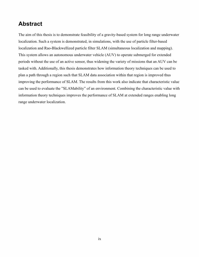
Abstract

The aim of this thesis is to demonstrate feasibility of a gravity-based system for long range underwater

localization. Such a system is demonstrated, in simulations, with the use of particle filter-based

localization and Rao-Blackwellized particle filter SLAM (simultaneous localization and mapping).

This system allows an autonomous underwater vehicle (AUV) to operate submerged for extended

periods without the use of an active sensor, thus widening the variety of missions that an AUV can be

tasked with. Additionally, this thesis demonstrates how information theory techniques can be used to

plan a path through a region such that SLAM data association within that region is improved thus

improving the performance of SLAM. The results from this work also indicate that characteristic value

can be used to evaluate the ”SLAMability” of an environment. Combining the characteristic value with

information theory techniques improves the performance of SLAM at extended ranges enabling long

range underwater localization.

x

List of Abbreviations and Symbols Used

Adj adjugate of a matrix

AUV autonomous underwater vehicles

a priori an existing map used as a reference

DR dead-reckoning

DVL Doppler velocity log

EM electromagnetic

Gal unit of gravity measurement (1 Gal = 1 cm s-2)

GPS Global Positioning System

IC individual compatibility

INS inertial navigation system

interpolation estimation within the range of a discrete set of known data points

LBL long baseline

MBE multi-beam echo sounder

multimodal a distribution with two or more distinct high values

nm nautical mile

NN nearest neighbour

online SLAM seeks to recover only the most recent pose

PMF point mass filter

SBL short baseline

SSBL super short baseline

SFM structure from motion

SIFT scale invariant feature transform

SLAM simultaneous localization and mapping

SPKF sigma point Kalman filter

TERCOM Terrain Contour Matching

TOF time-of-flight

USBL ultra short baseline

UUV unmanned underwater vehicles

xi

unimodal a distribution with a single highest value

𝑏𝑒̅̅ ̅𝑙(𝑥𝑡) prediction of state at time t

𝑏𝑒𝑙(𝑥𝑡) updated belief of state at time t

c speed of sound in water

𝐷𝑙 = ⟨𝑑1,d2,...,dnl⟩ output message containing the detected status of each cell (1 or 0)

𝐷𝑖𝑠𝑡Diagonal (𝑥𝑖,xgoal) diagonal distance from 𝑥𝑖 to goal node xgoal

f frequency (Hz = s-1)

𝑓(𝑥𝑖) cost function for node 𝑥𝑖

𝑓(𝑥𝑡−1, 𝑢𝑡, 휀𝑡) process equation f that provides the current state given the previous state,

control input and the process noise

�̅� gravity vector at an arbitrary location on earth

𝐻(𝑀𝑙) entropy of the message prior

𝐻𝑝(𝑥) entropy of probability distribution, p

ℎ (𝑥𝑖,xgoal) heuristic cost from node 𝑥𝑖 to goal node xgoal

ℎ(𝑥𝑡, 𝛿𝑡) measurement at time t given the current state and the measurement noise

𝐼(𝑀𝑙;d1) mutual information between channel input d1 and channel output M𝑙

InfoGain(𝑥𝑖) expected information gain from travelling to node 𝑥𝑖

M = ⟨𝑀1,M2,...,M𝐿⟩ inntended message containing the status of each cell (1 or 0)

𝑚 number of total landmarks

mi vector describing the location of the ith landmark whose true location is

assumed time invariant

𝑃𝐶𝐿 probability that all cells are occupied

PD probability of detection

PF probability of failure

𝑃𝑀𝑙 probability that the cell, 𝑀, is occupied

pose location of the robot, represented using the state vector 𝑥𝑡 = [𝑥, 𝑦, 𝜃]

𝑝(𝑥 |𝑦) = 𝑝(𝑋 = 𝑥 |𝑌 = 𝑦) probability that X’s value is x conditioned on the fact that Y’s value is y

𝑟 range

𝑈0:𝑘 history of control inputs

u control input

uk: control vector applied at time k-1 to drive the vehicle to a state xk at time k

xii

𝑤𝑡[𝑚]

weight of particle m at time t for a particle filter

𝑋0:𝑘 history of vehicle locations

𝑥 AUV longitude location

xk: state vector for particle k where 𝑥𝑘 = [𝑥, 𝑦, 𝜃] where [x, y] is the 2D location

and 𝜃 is the orientation

𝑥𝑡 state at time t

𝑦 AUV latitude location

𝑍0:𝑘 set of all landmark observations

𝑧 AUV depth

zik an observation from the vehicle of the location of the ith landmark at time k

zt measurement at time t

𝑧𝑡[𝑘]

predicted observation for particle k at time t

𝛿𝑠𝑘𝑖𝑛 skin depth

𝛤𝑘 characteristic parameter k grid steps away

𝛹 AUV heading

ℑ time-of-flight (TOF)

𝛻𝑔𝑛 gravity vector gradient

𝜋(𝑏) greedily optimized for belief b over all control inputs u

xiii

Acknowledgements

I would like to thank my thesis supervisors Dr. Mae L. Seto and Dr. Jason J. Gu for guiding me through

this project. It is not exaggeration to say that I would not have completed this thesis without their

mentorship and assistance. I would also like to thank my employer, Royal Canadian Navy, for the

tuition funding, and the supervisors who allowed me the flexibility to attend classes and dedicate time

to this thesis, particularly Lt(N) David Hogenbirk, LCdr(retd) Philippe Larrivee, LCdr Shawn Stacey

and LCdr Drew Matheson. And finally, I would like to thank my partner Dr. Carmen Nguyen for

putting up with my endless frustrations, helping edit this thesis and providing meaningful feedback.

1

Chapter 1 Introduction

Recent advances in robotics are enabling technologies for a wide range of applications in the maritime

environment. The field of autonomous systems and in particular, autonomous underwater vehicles

(AUVs), also commonly referred to as Unmanned Underwater Vehicles (UUVs), has been a rapidly

growing area of research. AUVs or UUVs can be used for a wide range of oceanographic and military

tasks such as underwater surveying, inspection of underwater structures, and laying undersea cables.

Applications previously requiring large investments in equipment and personnel are being considered

for execution using AUVs. The best developed example is that of naval mine counter-measures (Sariel,

Balch, & Erdogan, 2008) (O'Rourke, 2019). A broader range of applications has brought with it

additional requirements for AUVs. Increasingly, marine robots are expected to perform longer and

more complex missions, respond to dynamic environments, perform missions that only an AUV can

complete and co-operate with other maritime assets (Seto, 2013). This is expected to be performed with

increasingly more adaptability. A key enabling technology for these wide range of applications is the

ability to navigate and localize.

Given the difficult underwater environment (poor underwater communications) and lack of positional

references, navigation and localization are critical capabilities in any kind of mission that an AUV may

be tasked with. Whether the AUV is conducting an oceanographic survey or trying to identify mines in

a minefield, the AUV needs to localize itself to within a small error and navigate well to geo-reference

its sensors’ measurements.

Localization is particularly challenging underwater due to limitations in the medium. Electromagnetic

(EM) signals, including those from GPS, do not propagate far underwater. Therefore, an AUV must

rely on an onboard inertial navigation system (INS) to localize itself while submerged. Depending on

the mission, an INS that meets the accuracy requirement might be expensive with costs of up to

hundreds of thousands of dollars. The AUV can surface periodically to reduce its position error through

a GPS calibration but depending on the type of mission that the AUV is tasked with, for example

under-ice localization and navigation, this might not be an option. Another option is for the AUV to use

on-board acoustic modems to communicate with buoys or other ships, that know their position well, to

localize itself. The disadvantage of this baseline-based localization is that it requires external

infrastructure to assist the AUV, defeating one of the main reasons for employing an autonomous

2

platform. The preferred option is to employ a sensor onboard that can assist with localization. This

would limit the error growth of the onboard INS and keep the error within the requirements of the

mission. The ideal sensor would be low cost, accurate, and minimizes the localization error.

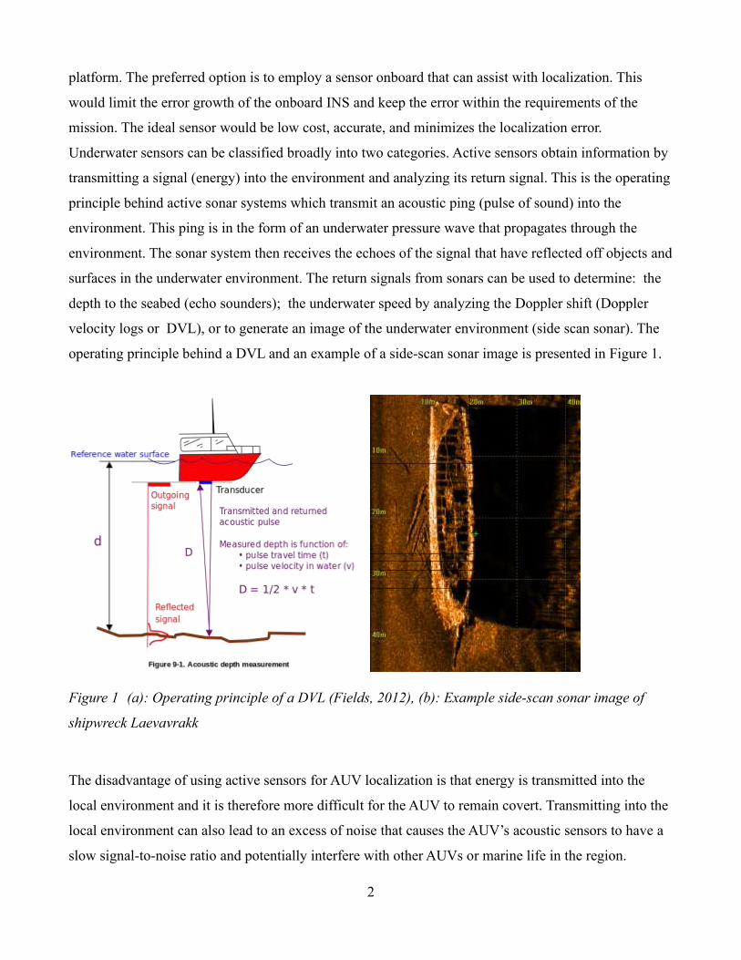
Underwater sensors can be classified broadly into two categories. Active sensors obtain information by

transmitting a signal (energy) into the environment and analyzing its return signal. This is the operating

principle behind active sonar systems which transmit an acoustic ping (pulse of sound) into the

environment. This ping is in the form of an underwater pressure wave that propagates through the

environment. The sonar system then receives the echoes of the signal that have reflected off objects and

surfaces in the underwater environment. The return signals from sonars can be used to determine: the

depth to the seabed (echo sounders); the underwater speed by analyzing the Doppler shift (Doppler

velocity logs or DVL), or to generate an image of the underwater environment (side scan sonar). The

operating principle behind a DVL and an example of a side-scan sonar image is presented in Figure 1.

Figure 1 (a): Operating principle of a DVL (Fields, 2012), (b): Example side-scan sonar image of

shipwreck Laevavrakk

The disadvantage of using active sensors for AUV localization is that energy is transmitted into the

local environment and it is therefore more difficult for the AUV to remain covert. Transmitting into the

local environment can also lead to an excess of noise that causes the AUV’s acoustic sensors to have a

slow signal-to-noise ratio and potentially interfere with other AUVs or marine life in the region.

3

Passive sensors obtain information about the environment without putting energy into the water.

Examples of this are passive sonar arrays, magnetometers, video cameras, etc. The advantage of a

passive sensor is that no energy is transmitted into the environment, allowing the AUV to remain

undetected. The disadvantage is that passive sensors generally require additional processing to obtain

information.

In this work, localization and navigation using gravity-based sensors is considered for use onboard

AUVs. This type of passive sensor has a number of advantages that make them ideal for underwater

navigation, including low cost and stability over time. The focus of this thesis is on using gravity-based

sensors to perform long-range localization and navigation onboard AUVs. The intent is for this thesis to

act as a starting resource for researchers and engineers interested in implementing gravity-based sensor

systems in AUVs.

This thesis examines the use of gravity anomaly measurements to perform localization using Rao-

Blackwellized particle filter-based localization (Pasnani & Seto, 2018). A gravimeter sensor provides a

scalar reading of the local gravity anomaly value, which is a measure of the gravitational acceleration’s

deviation, at the current AUV pose, from the standard “ellipsoid” model of Earth (Schubert, 2015). A

gradiometer measures the spatial rate of change of the gravitational acceleration. By combining both

measurements, it is possible to localize the gravimeter/gradiometer to a position on Earth (Jircitano,

White, & Dosch, 1990). This is a challenging task for two major reasons. Firstly, the gravity

measurement is sensitive and current sensor measurements allow for a precision of only about 4.5

mGal (Biebauer, 2015) (Middlemiss, et al., 2016). Secondly, the best gravity anomaly maps that are

publicly available are from the Scripps Institution of Oceanography (SIO), which have a spatial

resolution of approximately 1 nm × 1 nm (Sandwell, Muller, Smith, & Francis, 2014). In (Pasnani &

Seto, 2018), we showed that an a priori map of the gravity measurements within a region can be

combined with sensor measurements and a particle filter-based algorithm to provide near real-time

localization. The possibility of applying a simultaneous localization and mapping (SLAM) based

approach was not addressed in our publication but it will be in this thesis.

A SLAM-based approach to long-range localization would provide advantages over traditional

localization methodologies. A SLAM-based approach using gravity anomaly measurements considers

4

the sensor error and the uncertainty of the motion to provide a refined estimate of the robot’s location.

By performing SLAM, some of the limitations of the low-resolution gravity anomaly map available

from the SIO can be overcome by building a local map of the environment as the AUV travels through

it. The challenge with applying a SLAM-based approach is that there is no relationship between the

gravimeter measurement and the pose of the robot. This is because to determine a position on Earth

from a single gravity measurement, the robot must compare the measurement to an existing database of

measurements. If a sensor model could be developed, state estimation techniques like an extended

Kalman filter (EKF) could be used to address with the non-linearity of the model. A few different

approaches have been developed to overcome this challenge. The article (Xiong, Ma, & Tian, 2011)

used neural networks to obtain a position estimate from a gravity measurement. Another article (Wang

& Bian, 2008) proposed using a geopotential model to develop the measurement model. In the

literature, the standard approach has been to use some version of scan matching such as iterative closest

contour point (ICCP) (Jircitano, White, & Dosch, 1990) which is similar to Terrain Contour Matching

(TERCOM) (Han, Wang, Deng, & Fu, 2016) to localize the vehicle against an existing map.

To perform localization using gravity anomaly values, we develop a particle filter-based localization

solution. The sparse 1 nm × 1 nm gravity anomaly measurement map available from the SIO is treated

as landmarks in the environment. These landmarks can be used to restrict the growth of the position

error. This means our algorithm has to localize the AUV to much better than 1 nm. The hypothesis is

that by using these existing observations with our SLAM algorithm, we can achieve long-range

localization in GPS denied environments. The purpose of this thesis was twofold. One, to demonstrate

the feasibility of particle filter-based localization in such an environment by using a “novel”

observation model. Secondly, to show that the performance of such an algorithm is dependent on the

local gravity anomaly environment. The goal is to develop a predictive model of this performance so

that it can perform path-planning for AUV missions. Both of these will bring us closer to the goal of

this thesis, which is to improve long-range underwater localization and navigation onboard AUVs using

gravity-based measurements.

The contributions from this thesis are to demonstrate the use of gravity-based sensor to perform

underwater localization and navigation. Motivated by conducting localization over long ranges,

information theory techniques were applied to analyze the navigability of different regions. Information

theory techniques were also applied to evaluating the suitability of an environment for conducting

5

SLAM. A gravity-based SLAM system was implemented. The results from the gravity-based SLAM

system demonstrated the effectiveness of using information theory techniques to evaluate the

“SLAMability” of different environments.

The rest of this thesis is organized as follows. Chapter 2 conducts a review of the theoretical basis for

localization, navigation and SLAM with a focus on the techniques applied in this thesis. Chapter 3

explains the motivation for the problem and identifies the key metrics that this thesis aims to advance.

Chapter 4 reviews gravity-based sensors and the fundamentals of SLAM. Chapter 5 discusses how the

problems identified Chapter 3 are solved. Chapter 6 analyzes the results of the proposed solutions.

Chapter 7 discusses how these results are relevant. Chapter 8 provides direction on how the solutions

proposed in this thesis could be extended and applied to different applications in the future. Chapter 9

summarizes the key findings and novel contributions of this thesis.

6

Chapter 2 Literature Review

2.1 Localization Review

AUV localization is a fast-evolving field with significant research devoted to solving the problem of

underwater navigation and localization. Localization is particularly challenging underwater due to the

nature of the environment. With active sensors, communications is a fundamental aspect of localization

and navigation. High frequency electromagnetic (EM) signals like those used for GPS cannot penetrate

underwater much further than the surface (Seto, 2013). This is due to the high permittivity and

electrical conductivity of water. For a given frequency, f, and electrical conductivity, σ, the distance an

EM signal travels underwater is given by 𝛿𝑠𝑘𝑖𝑛, the skin depth (m) (Che, Wells, Dickers, Kear, & Gong,

2010) defined as follows:

𝛿𝑠𝑘𝑖𝑛 = 1/(2π √𝑓𝜎 𝑋 10−7). (1)

For sea water, typical conductivities range from 3.2 to 5.4 S/m with the resultant propagation distances

ranging from 323 m at 100 Hz to 0.7 m at 10 MHz. The propagation speed of the EM waves in sea

water is given as below (Balanis, 2012).

𝑐 ≈ √4πf

μσ . (2)

Since the propagation speed of the EM waves is proportional to the square root of its frequency, lower

frequency waves travel further and slower in sea water. This has important implications not only for

underwater communications but also for sensing technologies that rely on EM waves. The best suited

technology for underwater communications is acoustic-based communications due to its relatively low

absorption in water. Nevertheless, underwater acoustic propagation still has significant challenges,

which significant research is dedicated to overcoming. With an understanding of the challenges that the

underwater domain inherently poses, an overview of the kind of localization technologies currently

available can be conducted.

AUV navigation and localization techniques can be broken down into three major categories (Paull,

Saeedi, Seto, & Li, 2014):

7

• Inertial/dead reckoning: Onboard accelerometers and gyroscopes are used to propagate the

current state. The major pitfall of this approach is that the position error growth is unbounded.

• Acoustic transponders and modems: The vehicle uses acoustic beacons or modems to measure

time-of-flight to perform localization. This requires a localization beacon or a support ship.

• Geophysical: A sensor is used to obtain external environment information to use as references

for localization and navigation. It requires using sensors that are capable of identifying and

classifying environmental features.

2.1.1 Inertial/Dead Reckoning

To begin, key definitions of the basics of localization are presented. These terms will be used to define

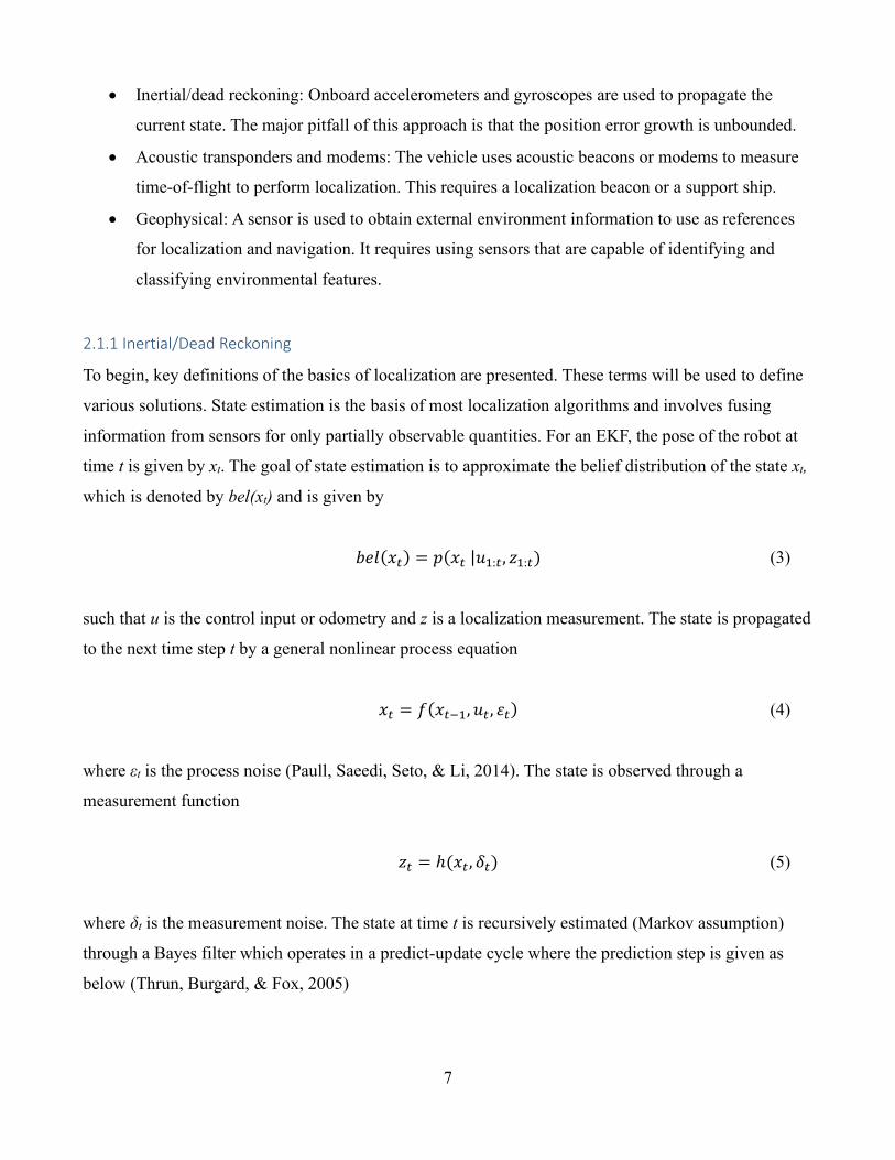
various solutions. State estimation is the basis of most localization algorithms and involves fusing

information from sensors for only partially observable quantities. For an EKF, the pose of the robot at

time t is given by xt. The goal of state estimation is to approximate the belief distribution of the state xt,

which is denoted by bel(xt) and is given by

𝑏𝑒𝑙(𝑥𝑡) = 𝑝(𝑥𝑡 |𝑢1:𝑡, 𝑧1:𝑡) (3)

such that u is the control input or odometry and z is a localization measurement. The state is propagated

to the next time step t by a general nonlinear process equation

𝑥𝑡 = 𝑓(𝑥𝑡−1, 𝑢𝑡 , 휀𝑡) (4)

where εt is the process noise (Paull, Saeedi, Seto, & Li, 2014). The state is observed through a

measurement function

𝑧𝑡 = ℎ(𝑥𝑡, 𝛿𝑡) (5)

where δt is the measurement noise. The state at time t is recursively estimated (Markov assumption)

through a Bayes filter which operates in a predict-update cycle where the prediction step is given as

below (Thrun, Burgard, & Fox, 2005)

8

𝑏𝑒̅̅ ̅𝑙(𝑥𝑡) = ∑ 𝑝(𝑥𝑡|𝑥𝑡−1,u𝑡) bel(𝑥𝑡−1)𝑥𝑡−1. (6)

The update step is then

𝑏𝑒𝑙(𝑥𝑡) = 𝜂𝑝(𝑧𝑡|𝑥𝑡)𝑏𝑒𝑙̅̅ ̅̅ (𝑥𝑡) (7)

where 𝜂 is the normalization factor. In simple terms, the Bayes filter can be thought of as follows. The

current position is predicted based on the previous position and the last odometry input. The prediction

is then adjusted based on measurements made of the environment.

State estimation relies on the Markov assumption, which states that only the most recent state

estimates, control, and measurements need to be considered to generate the estimate of the next state.

Effects such as unmodelled dynamics in the environment, relationships between the past measurements

and the future measurements can cause the Markov assumption to be violated. In principle, these

variables can be included in state representations. However, incomplete state representations allow for

the practical implementation of SLAM by reducing its computational complexity (Thrun, Burgard, &

Fox, 2005). The general state estimation process is shown in Figure 2, and some of the most common

state estimation techniques are described below.

Figure 2 State estimation process (Stachniss, 2013)

9

The Kalman filter is probably the most popular technique for implementing a Bayes filter. In addition

to the Markov assumption of the Bayes filter, the Kalman filter requires that the following three

properties hold in order to calculate a Gaussian posterior. One, the state transition probability

𝑝(𝑥𝑡|𝑢𝑡,x𝑡−1) must be a linear function. Second, the measurement probability 𝑝(𝑧𝑡|𝑥𝑡) must also be

linear. Third, the initial belief distribution, or prior, 𝑏𝑒𝑙(𝑥0) = 𝑝(𝑥0) must be normally distributed.

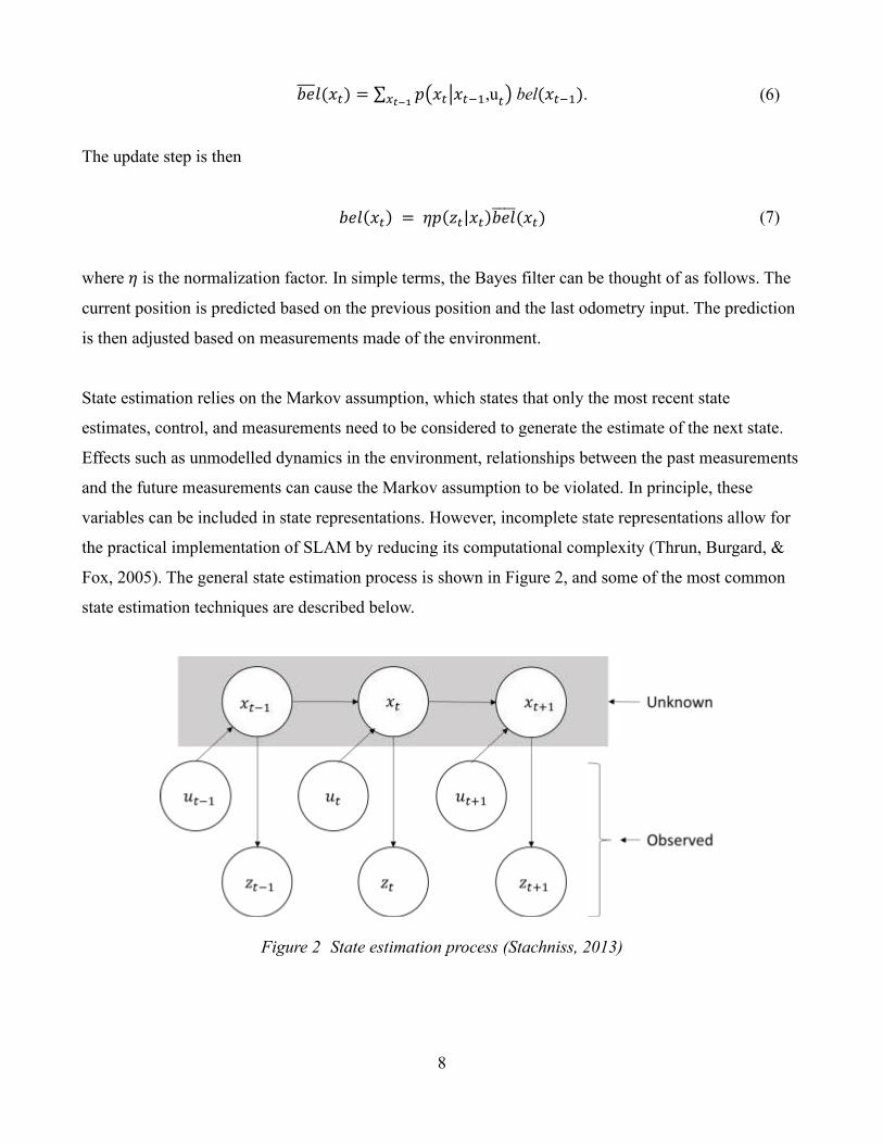
Dead-reckoning (DR) is the process of estimating the current pose based upon knowledge of the

previous pose and the velocity or acceleration vector. The advantage of dead-reckoning is that it is a

straightforward method of pose estimation and the solution is optimal provided that the above three

conditions are met. State estimation algorithms can be used in conjunction with dead-reckoning to

localize the AUV more accurately. An information flow diagram of the dead-reckoning process is

shown in Figure 3.

Figure 3 Common dead-reckoning process (Paull, Saeedi, Seto, & Li, 2014) onboard an AUV

If a compass heading from a part of an inertial measurement unit (IMU) and velocity from a DVL are

available, then the following equations can be used for DR estimation:

𝑥 = 𝑣 cos 𝛹 + 𝑤 sin 𝛹

𝑦 = 𝑣 sin 𝛹 + 𝑤 cos 𝛹

𝛹 = 0

(8)

such that x, y, and Ψ are the change in the latitude, longitude, and heading, respectively. The

disadvantage of dead-reckoning is that the localization performance drifts over time. This is because of

10

the integration of the sensed accelerations from the IMU to yield positions or displacements. Since the

next position is calculated by integrating the previous position from the odometry inputs, the positional

error grows unbounded over time. A common approach is to include this drift as part of the robot’s state

(Miller, Farrell, Zhao, & Djapic, 2010). While this error can be reduced with increasing INS cost or

more complex design, it cannot be eliminated. Without an external position reference, the error grows

unbounded. Therefore, the performance of a DR algorithm depends on the performance of the INS.

However, as the performance of an INS increases so does its cost. The best INS has a drift rate of about

1% of the distance traveled while more typical units generally achieve a rate of 2 – 5% of the distance

traveled (Fallon, Kaess, Johannsson, & Leonard, 2011).

2.1.2 Acoustic Transponders and Modems

Acoustic means use time-of-flight (TOF) measurements of acoustic signals to localize the AUV. The

operating principle of acoustic localization is like that of GPS, trilateration. Range measurements are

made to multiple acoustic beacons which allows the AUV to determine its position from trilateration.

The most common methods are illustrated in Figure 4 and are described below.

Short Baseline (SBL) uses transceivers placed at either end (forward and aft) of a ship’s hull to

triangulate and localize the AUV. Time-of-flight measurements allow the AUV to determine its relative

bearing and range. SBL is like Ultrashort Baseline (USBL), which is also commonly called Super Short

Baseline (SSBL).

In USBL, AUV location is determined by measuring the TOF and phase differencing across an array of

transceivers. The disadvantage with both these methods is that a support ship is required to assist in the

localization. This means that the AUV must remain in constant communication with the support ship

and it is therefore limited in range and in the types of mission it can perform. The positional accuracy

depends on the size (length) of the baseline. Therefore, in SBL, the length of the ship limits the

positional accuracy that can be achieved. An example application was presented in (Ridao, Carreras,

Ribas, & Garcia, 2010) where USBL was appropriate for the task due to the limited range of the

mission. A buoy equipped with a differential GPS was used to improve the localization accuracy of an

AUV that performed analysis of a dam wall using video cameras. An extended Kalman filter was used

to fuse the visual data from the camera with the positional information onboard the AUV and the

measurements from the USBL.

11

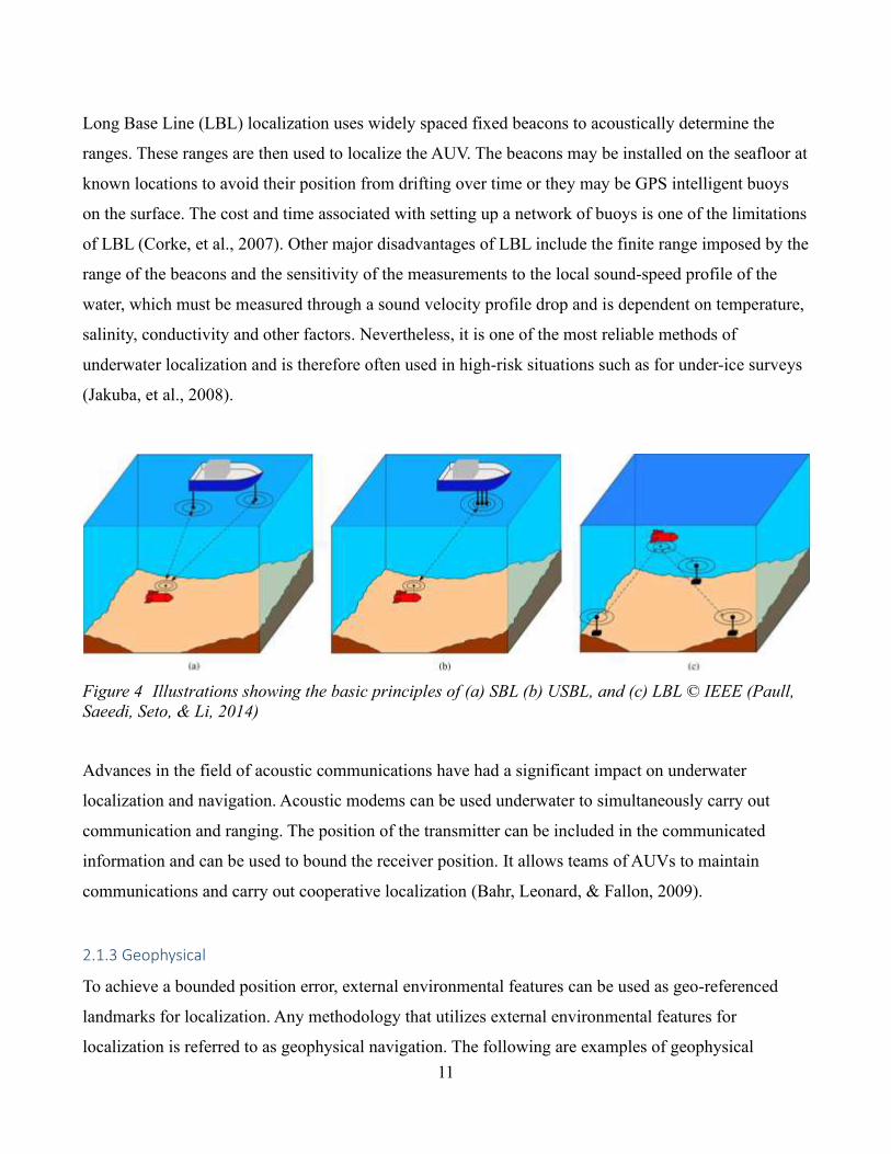
Long Base Line (LBL) localization uses widely spaced fixed beacons to acoustically determine the

ranges. These ranges are then used to localize the AUV. The beacons may be installed on the seafloor at

known locations to avoid their position from drifting over time or they may be GPS intelligent buoys

on the surface. The cost and time associated with setting up a network of buoys is one of the limitations

of LBL (Corke, et al., 2007). Other major disadvantages of LBL include the finite range imposed by the

range of the beacons and the sensitivity of the measurements to the local sound-speed profile of the

water, which must be measured through a sound velocity profile drop and is dependent on temperature,

salinity, conductivity and other factors. Nevertheless, it is one of the most reliable methods of

underwater localization and is therefore often used in high-risk situations such as for under-ice surveys

(Jakuba, et al., 2008).

Figure 4 Illustrations showing the basic principles of (a) SBL (b) USBL, and (c) LBL © IEEE (Paull,

Saeedi, Seto, & Li, 2014)

Advances in the field of acoustic communications have had a significant impact on underwater

localization and navigation. Acoustic modems can be used underwater to simultaneously carry out

communication and ranging. The position of the transmitter can be included in the communicated

information and can be used to bound the receiver position. It allows teams of AUVs to maintain

communications and carry out cooperative localization (Bahr, Leonard, & Fallon, 2009).

2.1.3 Geophysical

To achieve a bounded position error, external environmental features can be used as geo-referenced

landmarks for localization. Any methodology that utilizes external environmental features for

localization is referred to as geophysical navigation. The following are examples of geophysical

12

navigation. Additional sensing paradigms facilitate the development of better localization and

navigation methods.

Optical localization is implemented with either a monocular or stereo video camera to capture images

and then use these images to navigate with. In visual odometry, subsequent camera images are analyzed

to determine the robot’s pose. This can be done through optical flow or structure from motion (SFM)

algorithms. Algorithms developed for ground and air robotics, like scale-invariant feature transform

(SIFT), can be applied to underwater robots. In the underwater environment, the major limitations for

optical localization are the range and resolution of the cameras and light availability. Due to scattering

from suspensions in the water column, light does not travel far underwater. Therefore, optical

localization techniques are better suited for small scale feature-rich mapping of underwater

environments. An example of this was presented in (Eustice, Large-Area Visually Augmented

Navigation for Autonomous Underwater Vehicles, 2005) and (Eustice, Pizarro, & Sing, Visually

Augmented Navigation for Autonomous Underwater Vehicles, 2008), where their underwater vision-

based SLAM, called Visually Augmented Navigation (VAN), was implemented.

Sonar is one of the most common geophysical underwater localization and navigation methods. Sonar

can be used to acoustically identify and navigate based on detected features in the environment.

Typically, sonar is used in conjunction with SLAM-based methods for localization and navigation.

2.2 SLAM

Simultaneous Localization and Mapping aims to construct a map of the local environment while

simultaneously using the map to localize the robot within it. The concept of SLAM was first proposed

at the 1986 IEEE Conference on Robotics and Automation (Durrant-Whyte & Bailey, 2006). During

the conference a number of researchers acknowledged that it was a fundamental problem in robotics

with major conceptual and computational issues to address. The fundamental challenge of SLAM is in

developing a map of the environment while at the same time localizing oneself on the map. Humans

naturally conduct SLAM in their daily lives when determining their location in a room, or for example,

when deciding which specific desk to use in the library. On a theoretical and conceptual level, SLAM is

considered a solved problem, however considerable work remains to allow for practical

implementations. There are several real-world situations where the algorithm breaks down either due to

the nature of the environment, the robot, or the performance requirements. Nevertheless, SLAM has

13

been applied to a number of different domains, from indoor to outdoor, from underwater to above water

with each domain bringing its own particular challenges and opportunities. The problems faced by

researchers in applying SLAM to different domains allows us to progress the state-of-the-art and

develop insight into SLAM. The ultimate aim is to develop a SLAM system that is capable of meeting

the key requirements of robust performance, high-level understanding, resource awareness, and task-

driven perception (Cadena, et al., 2016). A standard formulation and structure of SLAM is presented in

Chapter 4.

2.2.1 Bathymetric sonar

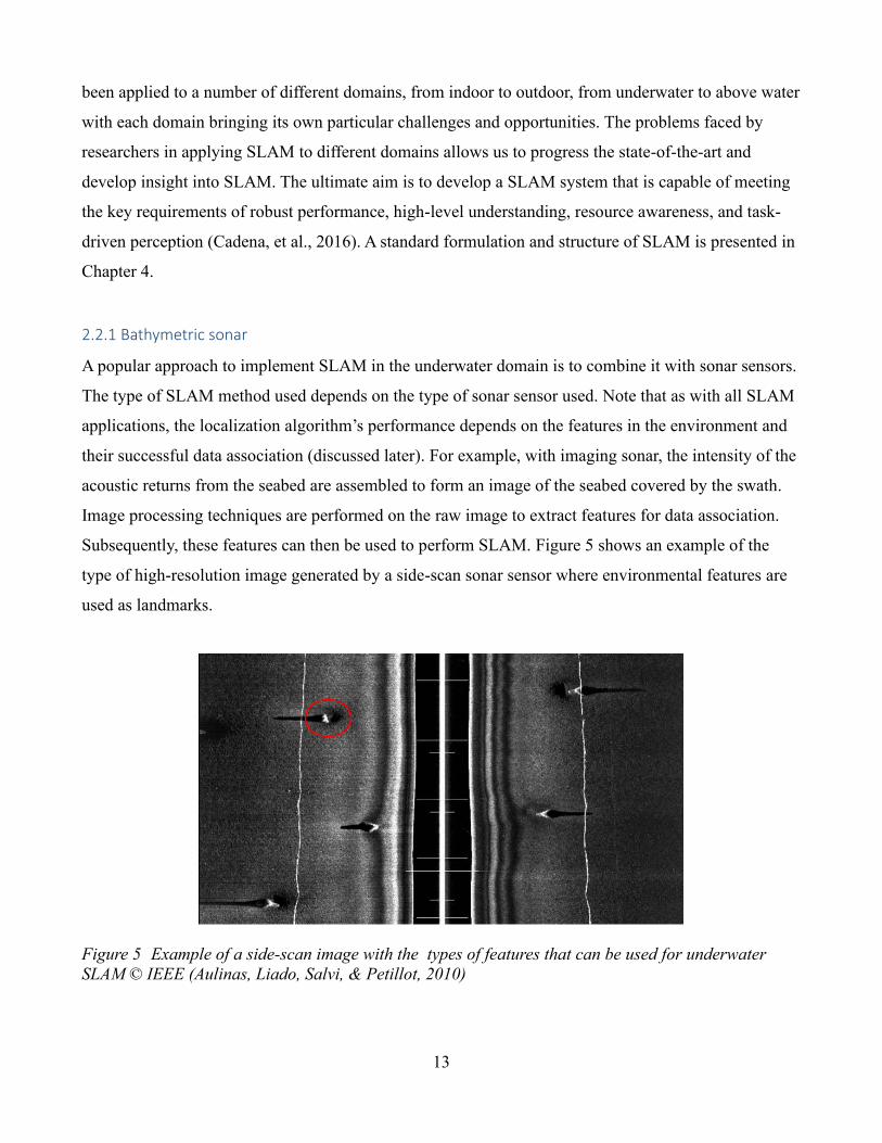
A popular approach to implement SLAM in the underwater domain is to combine it with sonar sensors.

The type of SLAM method used depends on the type of sonar sensor used. Note that as with all SLAM

applications, the localization algorithm’s performance depends on the features in the environment and

their successful data association (discussed later). For example, with imaging sonar, the intensity of the

acoustic returns from the seabed are assembled to form an image of the seabed covered by the swath.

Image processing techniques are performed on the raw image to extract features for data association.

Subsequently, these features can then be used to perform SLAM. Figure 5 shows an example of the

type of high-resolution image generated by a side-scan sonar sensor where environmental features are

used as landmarks.

Figure 5 Example of a side-scan image with the types of features that can be used for underwater

SLAM © IEEE (Aulinas, Liado, Salvi, & Petillot, 2010)

14

Another common approach is to use bathymetric features in the environment. A bathymetric map is an

elevation (or topographical) map of the underwater environment that is acquired with a multi-beam

sonar. Techniques developed for use in terrain-aided navigation can be applied to underwater

bathymetric navigation as well. The first terrain- based navigation techniques were developed for use

by aircrafts and missiles. In aerial vehicles, the barometric altitude and radar or laser altimetry are used

to obtain the height of the vehicle from the terrain. A profile of the terrain is then obtained which is

used towards localization and navigation (Melo & Matos, Survey on advances on terrain based

navigation for Autonomous Underwater Vehicles, 2017). In bathymetric navigation, the depth to the sea

floor is measured using multi-beam sonars from which features can be extracted and used for

navigation. The depth of the sea floor at any location is a combination of the AUV’s depth and the

depth below the vehicle. This can be written as:

𝑧 = 𝑧𝑣 + ℎ𝑣 + 𝑎𝑣. (9)

Here, 𝑧𝑣 is the depth of the vehicle, typically obtained using an onboard pressure sensor, ℎ𝑣 is the depth

of the sea floor from the water surface and 𝑎𝑣 is the distance between the pressure sensor and the depth

sensor. One way of conducting localization underwater is to use the information on the depth to the

seafloor from a single beam echosounder (SBE) sensor. An SBE measures the depth to the sea floor ℎ𝑣

at only one point, usually directly below the vehicle by transmitting a ping or sound pulse. The sound

pulse bounces of the sea floor and the time it takes for the echo to be received, known as the time-of-

flight of the pulse, is used to compute the range r as follows:

𝑟 =ℑ𝑐

2 (10)

such that ℑ is the TOF and c is the local speed of sound in water, which can be determined from a

sound velocity profile cast. By combining consecutive pings, a profile of the underwater terrain can be

built and then used to perform localization as was done in (Anonsen, 2010), (Bachmann & Williams,

2003), (Karlsson & Gustafsson, 2003) and (Melo & Matos, On the use of Particle Fitlers for Terrain

Based Navigation of sensor-limited AUVs, 2013). In (Teixeira, Pascoal, & Maurya, 2012), a depth

sonar-type sensor was combine with a DVL and a forward-looking sonar to provide a set of three range

measurements that could be used to estimate the AUV’s pose. Similar to an SBE, a multibeam

echosounder (MBE) measures the depth to the seafloor beneath the vehicle, but it uses multiple sonar

15

beams. The beams taken together cover a large area under the vehicle and can be used to build an

accurate high-resolution map of the sea floor. In (Nygren, 2005), Nygren demonstrates the use of a

MBE sonar for terrain-based navigation and demonstrated its robustness against different types of

measurement errors and map errors. In (Anonsen, 2010), terrain-aided navigation is applied to the

underwater domain using AUVs. Different types of terrain-aided navigation algorithms were tested,

including TERCOM, point mass filter (PMF), various particle filters, and the sigma-point Kalman filter

(SPKF), and it was found that PMF is the most accurate and robust algorithm.

While there has been considerable work in the domain of underwater localization and navigation, there

are still limitations to the types of tasks that an AUV can be reliably expected to perform. Modern

AUVs generally rely on a combination of dead-reckoning, surfacing periodically for a GPS fix, and

baseline-based methods of localization. From a practical standpoint, these methods may be sufficient

for a majority of cases. However, further development is needed to conduct submerged long-range

localization and navigation using passive sensors. This thesis contributes to this.

16

Chapter 3 Problem Statement

The problem presented here could have significant impact on how AUVs are employed. As discussed in

previous chapters, current underwater localization and navigation methods have drawbacks that limit

the type of missions that an AUV can conduct. By addressing the problem of long-range underwater

localization and navigation, AUVs would achieve the flexibility needed to allow their use in a wide

range of applications.

An important aspect of AUV employability is their ability to remain undetected. Currently, AUVs are

primarily employed for oceanographic observation and in military missions like naval mine

countermeasures and anti-submarine warfare (O'Rourke, 2019). In both domains, energy transmission

into the environment by the AUV can be undesirable. In a military context, if no energy is transmitted it

helps the platform remain covert. In an oceanography context, this ensures that there is minimal

interference with marine life in the area.

To provide a practical solution for long-range underwater AUV localization and navigation, a survey of

the current methods was conducted, and the results were presented in Chapter 2. Here, each method is

evaluated in terms of their suitability in addressing long-range underwater localization and navigation.

Firstly, dead reckoning using an onboard INS is considered. In dead-reckoning, the localization error

grows unbounded at a rate driven by the INS quality and the time interval that the dead-reckoning is

performed over. This is from the accumulation of error over time. The error in such a system grows

until reliable localization and navigation can no longer be conducted. Then, some means is needed to

calibrate or zero the positional error (e.g. a GPS fix). High quality INS that would allow the AUV to

remain submerged for long periods of time are prohibitively expensive (Paull, Saeedi, Seto, & Li,

2014). Research is underway to use aiding sensors like DVLs to slow down the error growth. However,

the aiding sensors would not eliminate the error growth.

Acoustic modems and transceivers have been successfully applied to underwater localization for a

number of applications (Corke, et al., 2007), (Jakuba, et al., 2008), (Newman & Leonard, 2003). To

conduct underwater localization with baseline methods, buoys or ships with acoustic transmission

capabilities must be deployed prior to an AUV navigating through the region. This adds a logistical

17

hurdle to AUV deployment and can be impractical for the missions that an AUV may be employed for

(e.g. under-ice).

In terms of geophysical navigation methods, bathymetric-based methods are commonly used. They

have been successfully demonstrated in (Anonsen, 2010), (Bachmann & Williams, 2003), (Karlsson &

Gustafsson, 2003), (Melo & Matos, On the use of Particle Fitlers for Terrain Based Navigation of

sensor-limited AUVs, 2013), (Teixeira, Pascoal, & Maurya, 2012), and (Nygren, 2005). Their main

drawback is the transmission of sonar beams (acoustic energy) into the water, which could compromise

stealth requirements for some AUV missions. The scarcity of underwater maps and flat-bottomed areas

are the disadvantages of terrain-aided navigation systems (Nygren, 2005). While more charting can

obtain underwater maps, flat-bottomed areas will challenge terrain-aided navigation due to the lack of

features and subsequent uncertainty associated with a position based on those measurements. This

problem is similarly encountered in the approach proposed in this thesis and preliminary solutions to

the problem will be presented.

Another form of geophysical localization and navigation that has gained interest in recent years is

magnetic field based. Magnetic field maps of the Earth’s gravitational field can be used for localization.

An indoor version of magnetic field based navigation was presented in (Vallivaara, Haverinen,

Kemppainen, & Roning, 2011), and more recent work is focusing on integrating this into AUVs for

outdoor applications (Tkhorenko, Pavlov, Karshakov, & Volkovitsky, 2018) (Quintas, Teixeira, &

Pascoal, 2018). Magnetic localization and navigation has a number of drawbacks that limit its

widespread use. As one approaches the poles, the magnetic flux lines converge and fluctuate

unpredictably so that magnetic landmarks are less reliable for localization and navigation. The

magnetic poles historically switch polarities every 200,000 to 300,000 years with occasionally more

frequent switches. Magnetic field-based localization and navigation is also impacted by large local

magnetic fields generated by metallic structures like ships and oil rigs. All of these drawbacks make

magnetic field-based localization and navigation unsuitable for long-ranges underwater.

Motivated by these limitations, gravity-based localization and navigation was considered. Unlike

bathymetry and magnetic field-based methods, the Earth’s gravitational field persists and is stable over

time. It only changes due to large-scale natural or manmade activities. Another advantage of gravity-

based localization and navigation is that gravimeters can passively sense the gravity field, thus

18

allowing an AUV to remain undetected while remaining submerged for long periods of time. While

there has been some recent interest in using gravity-based localization and navigation, this remains an

underexplored field and will be the subject of this thesis. The primary focus of this thesis is to advance

the state-of-the-art in long-range underwater AUV localization and navigation using gravity-based

methods.

Once a navigation system using gravity-based measurements, particle filters, and an a priori map was

implemented, we demonstrate a gravity-based SLAM localization and navigation system. Several

challenges arise from extending gravity-based measurements to a SLAM system. Firstly, due to the

nature of the gravity sensor, there is no way to obtain an estimate of a robot’s position without an a

priori map. This means an observation model cannot be developed and therefore an EKF gravity-based

SLAM system cannot be implemented. Gravity-based sensors are not as rich in information as a camera

or laser scanner. Each measurement by a gravity-based sensor provides a measurement of the gravity

anomaly and the gravity gradient. The major limitation is thus the sparse nature of the sensor readings

in publicly available gravity maps. In this thesis, the focus is on the development of an online SLAM

algorithm that seeks to recover the most recent pose of a robot.

19

Chapter 4 Background

To fully realize the value of AUVs, localization and navigation at extended ranges and durations

without surfacing is needed. Gravity was chosen as the primary method to achieve this goal. In this

section, the working principles of gravimeters and the types of gravimeters that would be suitable for

AUV implementation are presented. The theoretical background for particle filter-based localization

algorithms and SLAM will also be discussed with following sections describing the approach,

methodology, and results.

4.1 Gravity-Based Localization and Navigation

Gravity-based localization and navigation was first proposed by Albert Jircitano while working at Bell

Aerospace Textron (Jircitano, White, & Dosch, 1990), where advances in moving-based gravity

gradiometery motivated this concept. Moving-based gravity gradiometery refers to the ability to mount

gradiometers on mobile platforms like aircraft or ships. At the time, many advantages to such an

approach were identified. Gravity-based navigation would be similar to terrain-based navigation. The

low frequency geological content of the gravity signal could be used for initial large position

adjustments with higher frequency content used for more accurate position estimates. Unlike other

technologies, gravitational measurements are made without active transmissions and would therefore

allow an AUV to remain covert. Additionally, the stability of gravitational fields allows for the

accumulation of measurements over time leading to more detailed maps and more accurate localization

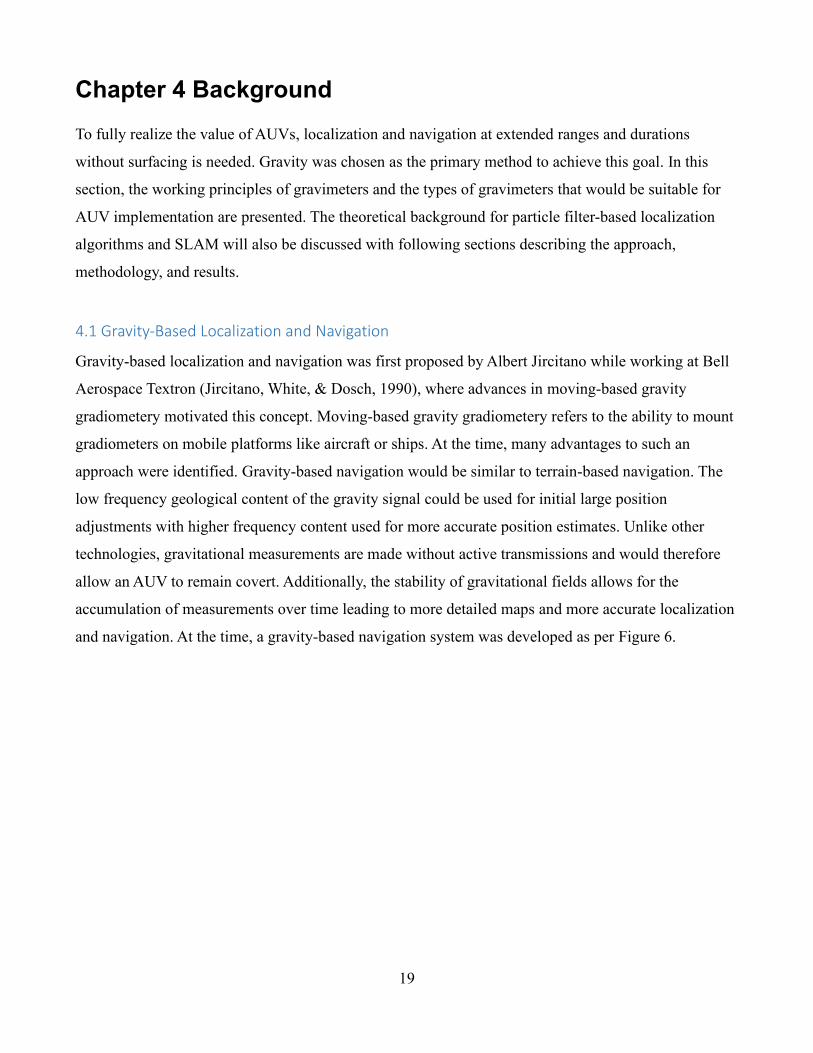
and navigation. At the time, a gravity-based navigation system was developed as per Figure 6.

20

Figure 6 Components of a gravity-based navigation system and the flow of information between them

Figure 6 shows how gravity-based navigation systems augment dead-reckoning with INS-based

localization and navigation. The platform senses the local gravitational field, matches the measurement

to a priori maps of the region, and then provides a correction to the dead-reckoned position from the

INS. This results in more accurate localization compared to a purely INS-based system. The a priori

map would be obtained from surveys of the region of interest over which localization and navigation is

to be conducted.

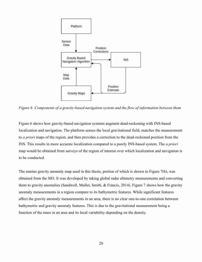
The marine gravity anomaly map used in this thesis, portion of which is shown in Figure 7(b), was

obtained from the SIO. It was developed by taking global radar altimetry measurements and converting

them to gravity anomalies (Sandwell, Muller, Smith, & Francis, 2014). Figure 7 shows how the gravity

anomaly measurements in a region compare to its bathymetric features. While significant features

affect the gravity anomaly measurements in an area, there is no clear one-to-one correlation between

bathymetric and gravity anomaly features. This is due to the gravitational measurement being a

function of the mass in an area and its local variability depending on the density.

21

4.1.1 Gravimeters

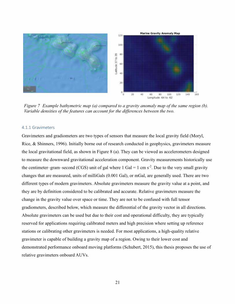
Gravimeters and gradiometers are two types of sensors that measure the local gravity field (Moryl,

Rice, & Shinners, 1996). Initially borne out of research conducted in geophysics, gravimeters measure

the local gravitational field, as shown in Figure 8 (a). They can be viewed as accelerometers designed

to measure the downward gravitational acceleration component. Gravity measurements historically use

the centimeter–gram–second (CGS) unit of gal where 1 Gal = 1 cm s-2. Due to the very small gravity

changes that are measured, units of milliGals (0.001 Gal), or mGal, are generally used. There are two

different types of modern gravimeters. Absolute gravimeters measure the gravity value at a point, and

they are by definition considered to be calibrated and accurate. Relative gravimeters measure the

change in the gravity value over space or time. They are not to be confused with full tensor

gradiometers, described below, which measure the differential of the gravity vector in all directions.

Absolute gravimeters can be used but due to their cost and operational difficulty, they are typically

reserved for applications requiring calibrated meters and high precision where setting up reference

stations or calibrating other gravimeters is needed. For most applications, a high-quality relative

gravimeter is capable of building a gravity map of a region. Owing to their lower cost and

demonstrated performance onboard moving platforms (Schubert, 2015), this thesis proposes the use of

relative gravimeters onboard AUVs.

Figure 7 Example bathymetric map (a) compared to a gravity anomaly map of the same region (b).

Variable densities of the features can account for the differences between the two.

22

Since the invention of the first gravity meters in the 1600s, which consisted of a pendulum on a wire,

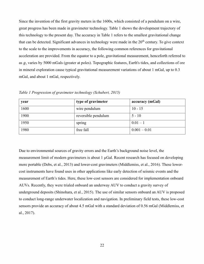
great progress has been made in gravimeter technology. Table 1 shows the development trajectory of

this technology to the present day. The accuracy in Table 1 refers to the smallest gravitational change

that can be detected. Significant advances in technology were made in the 20th century. To give context

to the scale to the improvements in accuracy, the following common references for gravitational

acceleration are provided. From the equator to a pole, gravitational measurement, henceforth referred to

as 𝑔, varies by 5000 mGals (greater at poles). Topographic features, Earth's tides, and collections of ore

in mineral exploration cause typical gravitational measurement variations of about 1 mGal, up to 0.3

mGal, and about 1 mGal, respectively.

Table 1 Progression of gravimeter technology (Schubert, 2015)

year type of gravimeter accuracy (mGal)

1600 wire pendulum 10 - 15

1900 reversible pendulum 5 - 10

1950 spring 0.01 – 1

1980 free fall 0.001 – 0.01

Due to environmental sources of gravity errors and the Earth’s background noise level, the

measurement limit of modern gravimeters is about 1 µGal. Recent research has focused on developing

more portable (Debs, et al., 2013) and lower-cost gravimeters (Middlemiss, et al., 2016). These lower-

cost instruments have found uses in other applications like early detection of seismic events and the

measurement of Earth’s tides. Here, these low-cost sensors are considered for implementation onboard

AUVs. Recently, they were trialed onboard an underway AUV to conduct a gravity survey of

underground deposits (Shinohara, et al., 2015). The use of similar sensors onboard an AUV is proposed

to conduct long-range underwater localization and navigation. In preliminary field tests, these low-cost

sensors provide an accuracy of about 4.5 mGal with a standard deviation of 0.56 mGal (Middlemiss, et

al., 2017).

23

4.1.2 Gradiometers

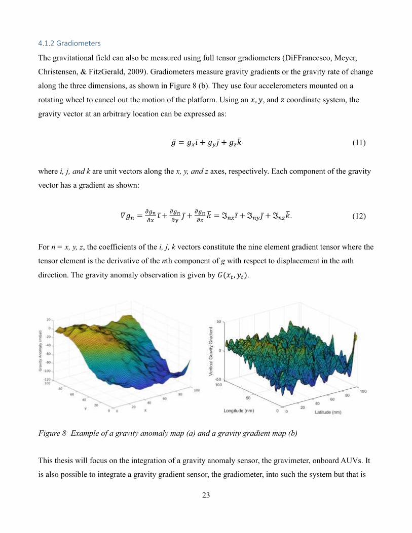
The gravitational field can also be measured using full tensor gradiometers (DiFFrancesco, Meyer,

Christensen, & FitzGerald, 2009). Gradiometers measure gravity gradients or the gravity rate of change

along the three dimensions, as shown in Figure 8 (b). They use four accelerometers mounted on a

rotating wheel to cancel out the motion of the platform. Using an 𝑥, 𝑦, and 𝑧 coordinate system, the

gravity vector at an arbitrary location can be expressed as:

�̅� = 𝑔𝑥𝑖̅ + 𝑔𝑦𝑗̅ + 𝑔𝑧�̅� (11)

where i, j, and k are unit vectors along the x, y, and z axes, respectively. Each component of the gravity

vector has a gradient as shown:

𝛻𝑔𝑛 =𝜕𝑔𝑛

𝜕𝑥𝑖̅ +

𝜕𝑔𝑛

𝜕𝑦𝑗̅ +

𝜕𝑔𝑛

𝜕𝑧�̅� = ℑ𝑛𝑥𝑖̅ + ℑ𝑛𝑦𝑗̅ + ℑ𝑛𝑧�̅�. (12)

For n = x, y, z, the coefficients of the i, j, k vectors constitute the nine element gradient tensor where the

tensor element is the derivative of the nth component of g with respect to displacement in the mth

direction. The gravity anomaly observation is given by 𝐺(𝑥𝑡, 𝑦𝑡).

This thesis will focus on the integration of a gravity anomaly sensor, the gravimeter, onboard AUVs. It

is also possible to integrate a gravity gradient sensor, the gradiometer, into such the system but that is

Figure 8 Example of a gravity anomaly map (a) and a gravity gradient map (b)

24

left for future work. Data from both sensors could be fused to develop a more accurate map of the

environment as well as improve the performance of the SLAM data association.

Modern efforts at integrating gravity-based localization and navigation with AUVs has been sporadic.

The results in (Wang, Wu, Chai, Bao, & Wang, Location Accuracy of INS/Gravity-Integrated

Navigation System on the Basis of Ocean Experiment and Simulation, 2017) are the most recent

example of real-world experiments.

4.2 Fundamentals of SLAM

This section will present a standard formulation and structure of the SLAM algorithm, and the different

implementation methods will be compared. Following this, a review of SLAM implementations in

various domains will be presented while keeping in mind the fundamental problem that this paper aims

to tackle.

Consider a robot moving through an environment while taking relative observations of unknown

landmarks, the following quantities are defined (Durrant-Whyte & Bailey, 2006) with k denoting an

instance in time:

xk: state vector describing the location and orientation of the vehicle

uk: control vector, applied at time k-1 to drive the vehicle to the state xk at time k

mi: vector describing the location of the ith landmark whose true location is assumed to be time

invariant and

zik: an observation from the vehicle of the location of the ith landmark at time k.

The following sets are defined:

𝑋0:𝑘 = {𝑥0, 𝑥1, … , 𝑥𝑘} = {𝑋0:𝑘−1, 𝑥𝑘} : history of vehicle locations

𝑈0:𝑘 = {𝑢1, 𝑢2, … , 𝑢𝑘} = {𝑈0:𝑘−1, 𝑢𝑘} : history of control inputs

𝑚 = {𝑚1, 𝑚2, … , 𝑚𝑛} : set of all landmarks and

𝑍0:𝑘 = {𝑧1, 𝑧2, … , 𝑧𝑘} = {𝑍0:𝑘−1, 𝑧𝑘} : set of all landmark observations.

25

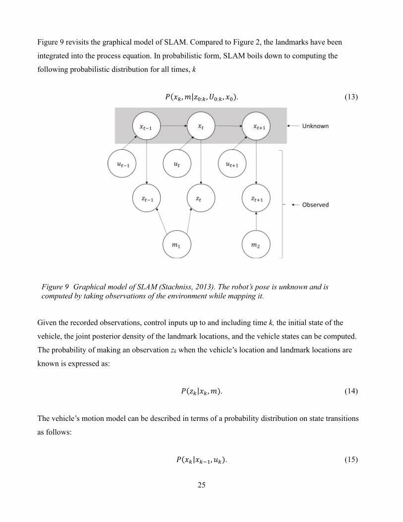
Figure 9 revisits the graphical model of SLAM. Compared to Figure 2, the landmarks have been

integrated into the process equation. In probabilistic form, SLAM boils down to computing the

following probabilistic distribution for all times, k

𝑃(𝑥𝑘, 𝑚|𝑧0:𝑘, 𝑈0:𝑘, 𝑥0). (13)

Given the recorded observations, control inputs up to and including time k, the initial state of the

vehicle, the joint posterior density of the landmark locations, and the vehicle states can be computed.

The probability of making an observation zk when the vehicle’s location and landmark locations are

known is expressed as:

𝑃(𝑧𝑘|𝑥𝑘, 𝑚). (14)

The vehicle’s motion model can be described in terms of a probability distribution on state transitions

as follows:

𝑃(𝑥𝑘|𝑥𝑘−1, 𝑢𝑘). (15)

Figure 9 Graphical model of SLAM (Stachniss, 2013). The robot’s pose is unknown and is

computed by taking observations of the environment while mapping it.

26

This assumes that the state transitions are Markov processes where the next state, xk, only depends on

the immediately preceding state xk-1 and the control input uk. The SLAM algorithm can be implemented

in a standard two-step recursive (sequential) form:

𝑃(𝑥𝑘, 𝑚|𝑍0:𝑘−1, 𝑈0:𝑘, 𝑥0)

= ∫ 𝑃(𝑥𝑘|𝑥𝑘−1,u𝑘) × 𝑃(𝑥𝑘−1,m|𝑍0:𝑘−1,U0:k−1,x0) dx𝑘−1

(16)

and in a prediction (time-update) form as:

𝑃(𝑥𝑘 , 𝑚|𝑍0:𝑘−1, 𝑈0:𝑘, 𝑥0) = 𝑃(𝑧𝑘|𝑥𝑘,m)𝑃(𝑥𝑘,m|𝑍0:𝑘−1,U0:k,x0)

𝑃(𝑧𝑘|𝑍0:𝑘−1,U0:k). (17)

The naive way of partitioning the joint posterior is not possible and leads to inconsistent results

(Durrant-Whyte H. , 1988). This is because observations depend on both the vehicle and landmark

locations, which are made explicit in the observation model. The most important insight in SLAM is

the realization that the correlations between landmark estimates increase monotonically as more

observations are made. This means that regardless of the robot’s motion, the joint probability density of

the landmarks becomes monotonically peaked as more observations are made. This is because

observations made by the robot can be considered “nearly independent” measurements of the relative

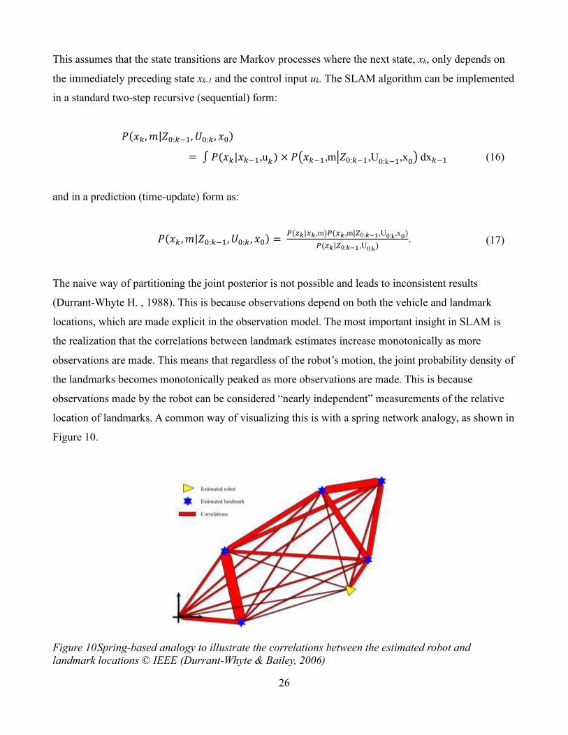
location of landmarks. A common way of visualizing this is with a spring network analogy, as shown in

Figure 10.

Figure 10 Spring-based analogy to illustrate the correlations between the estimated robot and

landmark locations © IEEE (Durrant-Whyte & Bailey, 2006)

27

The landmarks can be thought of as connected by springs, which represent the correlations between the

landmarks. As the robot moves through the environment, taking observations, the correlations increase,

and the springs get stiffer. This means that as the robot moves through the environment the error in the

estimates of the relative location between different landmarks reduces monotonically to the point where

the map of relative locations is known with absolute precision (Gamini, Newman, Clark, & Durrant-

Whyte, 2001). The theoretical limit of the robot’s location accuracy is equal to the error that existed

when the initial observation was made.

Finding a solution to the probabilistic SLAM problem involves finding an appropriate representation

for the observation and the motion models to allow computations of the prior and posterior distribution.

One of the most common representation is in the form on an EKF.

4.2.1 EKF

The EKF is the nonlinear version of the Kalman filter which combines previous measurements and a

system model to produce a more accurate estimate of noisy variables. A Kalman filter does this by

computing a predicted state and comparing this state with real-world measurements to generate a

Kalman gain. A standard Kalman filter requires linear system models that can be represented by normal

distributions. Optimal solutions can be obtained for (linear) problems that the Kalman filter models

well. Unfortunately, most interesting robotics problems cannot be modeled linearly. Therefore, the

EKF was developed to allow application of the Kalman filter to weakly nonlinear problems like

SLAM. The extended part of the EKF is achieved by expressing the nonlinear motion and/or

measurement model with a Taylor series expansion about the mean and covariance and retaining only

the first 2 terms. In EKF SLAM, the system model consists of the following functions

𝑥𝑘=f(𝑥𝑘−1,u𝑘)+w𝑘 and (18)

𝑧𝑘=h(𝑥𝑘)+v𝑘. (19)

The function f represents the predicted state at time k, which is calculated based on the previous state

estimate 𝑥𝑘−1 and the control input 𝑢𝑘. Similarly, the function h represents the predicted measurements

based on the predicted state. Here, 𝑤𝑘 and 𝑣𝑘 are the process and observation noise, respectively. The

28

two equations are the motion and the observation models and allow us to model the system and apply

the EKF.

The disadvantage of using EKF to solve the SLAM problem is that it linearizes systems that are

inherently nonlinear, leading to inconsistent or diverging solutions. Additionally, EKF SLAM can only

identify one likely solution to the problem as it still assumes normal probability distribution (unimodal)

functions are valid to capture the process and measurement. In situations where there may be multiple

hypotheses that should be maintained to identify the correct one as more information from the

environment becomes available, an EKF SLAM filter would estimate a solution between the two

hypotheses. EKF SLAM can lead to inconsistent loop closures and subsequent diverging solutions in

the event that landmarks are mis-identified (Rodriguez-Losada, Matia, Pedraza, Jimenez, & Galan,

2007). The main limitation that motivates the use of a Rao-Blackwellized particle filter (RBPF) in our

application is the requirement for a linearized system model in an EKF SLAM filter. A system model in

SLAM takes as input an observation about the environment and obtains a position estimate. With

gravity-based localization and navigation, due to the nature of the sensor, there is no straightforward

system model that could be developed. Once an observation is made, a position estimate is only

possible with an a priori map. The following chapters describe how our initial implementation used an

a priori map to perform localization. True SLAM does not require an a priori map. To overcome the

challenge of developing a system model, previous implementations have proposed using a geopotential

model (Wang & Bian, 2008) or a neural network-based model (Xiong, Ma, & Tian, 2011). Our final

implementation relies on a simple model that proved sufficient for our purposes and is further

discussed in the following chapters.

If system models cannot be developed, then Monte Carlo methods such as particle filters may be

employed. Particle filters fall under the category of nonparametric filters. Nonparametric filters do not

rely on a fixed analytical functional form for the posterior like Gaussian/normal distributions. Applying

particle filters to SLAM was first proposed by the seminal paper (Douce, Godsill, & Andrieu, 2000).

They approximate posteriors using a finite number of values corresponding to regions in space. This

allows them to represent multimodal beliefs and it makes them suitable for difficult data association

problems that may yield separate, distinct hypotheses. The accuracy of the approximation depends on

the number of particles used to represent the posterior. The greater the number of particles, the greater

the convergence to the correct posterior.

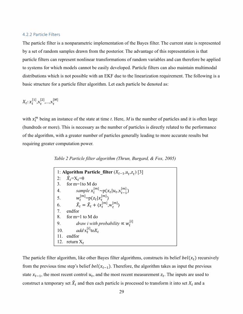
29

4.2.2 Particle Filters

The particle filter is a nonparametric implementation of the Bayes filter. The current state is represented

by a set of random samples drawn from the posterior. The advantage of this representation is that

particle filters can represent nonlinear transformations of random variables and can therefore be applied

to systems for which models cannot be easily developed. Particle filters can also maintain multimodal

distributions which is not possible with an EKF due to the linearization requirement. The following is a

basic structure for a particle filter algorithm. Let each particle be denoted as:

𝑋𝑡: 𝑥𝑡[1]

,x𝑡[2]

,...,x𝑡[𝑀]

with 𝑥𝑡𝑚 being an instance of the state at time t. Here, M is the number of particles and it is often large

(hundreds or more). This is necessary as the number of particles is directly related to the performance

of the algorithm, with a greater number of particles generally leading to more accurate results but

requiring greater computation power.

The particle filter algorithm, like other Bayes filter algorithms, constructs its belief 𝑏𝑒𝑙(𝑥𝑡) recursively

from the previous time step’s belief 𝑏𝑒𝑙(𝑥𝑡−1). Therefore, the algorithm takes as input the previous

state 𝑥𝑡−1, the most recent control 𝑢𝑡, and the most recent measurement 𝑧𝑡. The inputs are used to

construct a temporary set �̂�𝑡 and then each particle is processed to transform it into set 𝑋𝑡 and a

1: Algorithm Particle_filter (𝑋𝑡−1,u𝑡,z𝑡) [3]

2: �̂�𝑡=X𝑡=θ

3. for m=1to M do

4. sample 𝑥𝑡[𝑚]

∼p(𝑥𝑡|𝑢𝑡,x𝑡−1

[𝑚])

5. 𝑤𝑡[𝑚]

=p(𝑧𝑡|𝑥𝑡[𝑚]

)

6. �̂�𝑡 = �̂�𝑡 + ⟨𝑥𝑡[𝑚]

,w𝑡[𝑚]

⟩

7. endfor

8. for m=1 to M do

9. draw i with probability ∝ 𝑤𝑡[𝑖]

10. add x𝑡[𝑖]

to𝑋𝑡

11. endfor

12. return X𝑡

Table 2 Particle filter algorithm (Thrun, Burgard, & Fox, 2005)

30

posterior belief 𝑏𝑒𝑙(𝑥𝑡). In 𝑋𝑡, the higher the particle density in a region of state space, the more likely

it is that the true state falls into this region.

In line 5 of Table 2, the importance weight 𝑤𝑡[𝑚]

of each particle is calculated. The importance is the

probability of the measurement 𝑧𝑡 given the state 𝑥𝑡[𝑚]

. Once the set of particle weights is calculated,

the particle set is then resampled as per lines 8 through 11. During the resampling, particles are

sampled with replacement from the temporary set �̂�𝑡 with the likelihood that a particle is drawn based

on the probability of its importance weight. After resampling, the distribution of the particles in the

particle set is in proportion to their importance weight. The number of particles in the set remains the

same throughout all resamplings.

Particle filters have been applied to underwater terrain navigation by a number of different researchers

like (Bachmann & Williams, 2003), (Karlsson & Gustafsson, 2003), and (Melo & Matos, On the use of

Particle Filters for Terrain Based Navigation of sensor-limited AUVs, 2013). The advantage of particle

filters is that they can be applied directly to the nonlinear terrain-based localization and navigation

problem. However, one of the strengths of the particle filter can also be its downfall. That is, the ability

of a particle filter to maintain multi-modal belief also makes it susceptible to divergence if the wrong

mode is favored. If a sufficiently large number of particles are associated with the wrong mode, then

this is propagated through time and the true mode collapses. A significant contribution was made in

(Teixeira, Pascoal, & Maurya, 2012) by deriving two variants of an RBPF and demonstrating their

superiority in terms of position and velocity estimation when applied to terrain-based underwater

localization and navigation. In (Teixeira, Pascoal, & Maurya, 2012), the application of the described

methods to other forms of AUV localization and navigation was discussed, and the work presented in

this thesis builds on this previous work.

31

Chapter 5 Problem Setup

The work presented is focused on improving the performance of long-range underwater localization

and navigation in GPS-denied environments using a gravity-based sensor. While there has been

considerable research in conducting AUV localization and navigation at short ranges, they have

remained an underexplored topic. This may be partly due to the current lack of missions that would

drive such a need. However, with increasing use of autonomous platforms in all aspects of underwater

operations, these missions will become increasingly common with the ability to navigate being of

prime importance.

Currently, missions conducting under-ice operations are one of the few types of missions that have the

stringent set of requirements that this thesis attempts to address. Under-ice operations involve operating

in GPS-denied environments for extended ranges. For such operations, it may not be possible for the

AUV to surface. These types of mission include oceanographic surveys and laying fiber optic cables,

etc (O'Rourke, 2019). A notable example of a mission driving significant research in this field is the

polar expedition sponsored by the World Metrological Organization (Yu, Zhang, Li, & Yan, 2004). The

main mission of the polar expedition requires successful completion of a continuous 2000 km AUV

mission under the sea ice. This presents a significant challenge given current localization and

navigation technologies.

Previous efforts in this environment have relied on a combination of well calibrated INS and baseline-

based localization and navigation methods (Ferguson, 2009). In (Ferguson, 2009), localization errors of

less than 0.4% of the distance travelled with a 0.05% cross-track error was achieved. In (Kato &

Shigetomi, 2009), simulations were conducted over an area of the sea floor off the coast of Japan. Over

1000 km, it was shown that localization accuracy was best when localization and navigation was

performed using the geomagnetic and bathymetric map without an INS. The INS with a corrections

method performed almost as well and navigation conducted using only the INS performed worse.

Simulations conducted in (Salavasidis, et al., 2018) for over 3000 km were able to demonstrate

localization with error bounded to within 100 km. This constitutes an error of about 3% of the distance

travelled.

32

Due to the challenging nature of this problem domain and the current state of the field, the aim is to

achieve a localization accuracy of 5% of the distance. This means that to travel 100 nm underwater

without a GPS fix, the AUV would experience an average localization error of 5 nm.

The hypothesis is that this localization error could be achieved by incorporating gravity-based

measurements into the localization and navigation system. Firstly, in this thesis, the feasibility of such a

system using particle filters is demonstrated. A SLAM-based system is then demonstrated using

gravity-based measurements. A SLAM system has several advantages over a traditional system. Such a

system could operate without an a priori map and thus work in unfamiliar environments. A SLAM-

based system could also bound the growth of errors by conducting loop closure events allowing it to

trade-off between the distance travelled and the growth in localization uncertainty. The particle filter-

based localization and SLAM-based system are both simulated over long distances to characterize their

localization and navigation performance. At the long distances simulated, the performance of data

association, whether in the particle filter localization or in SLAM, has a significant impact on the

localization error.

In addition to demonstrating the feasibility of gravity-based localization and navigation, a method to

characterize the SLAM performance over a region is developed. By conducting simulations, it was

noted that the AUV operating region plays a major role in the outcome of the algorithms due to the data

association performance in that region. A major focus of this thesis was to develop a systemic method

to identify the “SLAMability” of a region of interest. This “SLAMability” metric would identify

regions with a high number of unique measurements prior to transiting through it, thus allowing for

greater overall localization and navigation performance.

The gravity-based SLAM system and “SLAMability” analysis are both novel contributions to the field.

5.1 Particle Filter-Based Localization and Mapping

Gravity-based localization and navigation has in principle been verified in previous work (Jircitano,

White, & Dosch, 1990) (Moryl, Rice, & Shinners, 1996) (Wang, et al., Characteristics of Marine

Gravity Anomaly Reference Maps and Accuracy Analysis of Gravity Matching-Aided Naviation,

2017). These previous works have demonstrated the feasibility of using gravity-based sensors. Initially,

as in the early work by Bell Aerospace (Jircitano, White, & Dosch, 1990), the sensor was part of the

33

INS, whereas more recent works use off-the-shelf gravimeters that are mounted on stabilized gimbal

platforms (Shinohara, et al., 2015). This thesis builds on these valuable works to demonstrate the

feasibility of a gravity-based system for long-ranges.

A particle filter-based formulation was chosen for this study. The non-parametric nature of the particle

filter allows the implementation of a particle filter-based localization algorithm with an a priori map. A

particle filter formulation also allows multiple hypotheses on a vehicle state. The AUV state is

described as:

𝑥𝑚,𝑡 = (𝑥1,𝑚,𝑡, 𝑥2,𝑚,𝑡, 𝑥3,𝑚,𝑡) (20)

where 𝑥1,𝑚,𝑡 and 𝑥2,𝑚,𝑡 are the AUV planar locations at a constant height (altitude) above the seabed,

and 𝑥3,𝑚,𝑡 is the heading Θ for particle m at time t. The particle filter propagates each particle through

the motion model 𝑓𝑡 in Equation 21:

𝑓𝑡 = [𝑥1,𝑚,𝑡

𝑥2,𝑚,𝑡] = [

𝑥1,𝑚,𝑡−1

𝑥2,𝑚,𝑡−1] + [

cos 𝑥3,𝑚,𝑡

sin 𝑥3,𝑚,𝑡] × 𝑢𝑡 × 𝑑𝑡 + 𝑤𝑡 (21)

such that 𝑢𝑡 is the constant AUV speed, dt is the time step, and 𝑤𝑡 is a 2 × 1 matrix ~ N(0, Q) as linear

Gaussian additive noise. The AUV position covariance matrix P is then 2 × 2.

Table 3 shows the particle filter algorithm used. The observation model h is a nonlinear function that

takes as input the robot state, 𝑥𝑚,𝑡, and the a priori map, 𝑀𝑗, as well as the sensor range, sensorRange.

From that, the observation model returns the measurement on the map that is closest to the AUV

position and within sensorRange. It returns the gravity measurement and the gravity gradient calculated

at that point if gravity landmark 𝑙𝑖 = [𝑙1, 𝑙2] where 𝑙1 and 𝑙2 are its (𝑥, 𝑦) locations with certainty

𝜎𝑙𝑎𝑛𝑑𝑚𝑎𝑟𝑘,𝑖. An extended Kalman filter update associates it with previously mapped landmarks through

individual compatibility (IC) and nearest neighbor (NN). This associates the landmark with the prior

mapped one that is most compatible. Firstly, IC rules out statistically unlikely data associations based

on the sum of the difference between the predicted and calculated gradients, i.e.:

min (∑ |𝑝𝑟𝑒𝑑𝑖𝑐𝑡𝑒𝑑(𝐺𝐺𝑖) − 𝑚𝑎𝑝𝑝𝑒𝑑 (𝐺𝐺𝑖)|4𝑖=1 . (22)

34

Then, of that subset, NN selects the best landmark based on the Mahalanobis distance:

mDisti = (𝑠𝑖,𝑚,𝑡 − 𝑙𝑖)𝑃−1

𝑑 = √∑ (𝑚𝐷𝑖𝑠𝑡𝑖

𝜎𝑙𝑎𝑛𝑑𝑚𝑎𝑟𝑘𝑖)22

𝑖=1 . (23)

If the landmark was previously observed and correctly associated, then the update improves the AUV

position state estimate and covariance. If the landmark was not previously observed, then its pose and

covariance are augmented into the prior map as a potential map improvement (Pasnani & Seto, 2018).

Simulations conducted for the localization system described above used the marine gravity anomaly

model “grav.img.24.1” (Sandwell, Muller, Smith, & Francis, 2014) from the Scripps Institution of

Oceanography. It has an accuracy of ± 3 – 8 mGal. Consequently, the combined uncertainty was taken

as ± 6 mGal for the analysis. The process uncertainty was taken to be 1% of the distance travelled. The

INS’s gyroscope was assumed to have angular noise with a standard deviation of 0.1 degrees. In the

analysis, the particle filter solution was compared to the “ground truth” solution obtained from a perfect

motion model implementation.

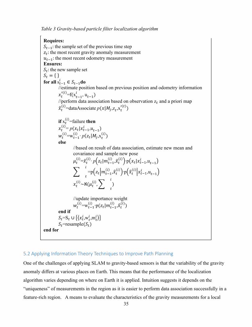
35

5.2 Applying Information Theory Techniques to Improve Path Planning

One of the challenges of applying SLAM to gravity-based sensors is that the variability of the gravity

anomaly differs at various places on Earth. This means that the performance of the localization

algorithm varies depending on where on Earth it is applied. Intuition suggests it depends on the

“uniqueness” of measurements in the region as it is easier to perform data association successfully in a

feature-rich region. A means to evaluate the characteristics of the gravity measurements for a local

Requires:

𝑆𝑡−1: the sample set of the previous time step

𝑧𝑡: the most recent gravity anomaly measurement

𝑢𝑡−1: the most recent odometry measurement

Ensures:

𝑆𝑡: the new sample set

𝑆𝑡 = { }

for all s𝑡−1𝑖 ∈ 𝑆𝑡−1do

//estimate position based on previous position and odometry information

𝑥𝑡′(𝑖)

=f(x𝑡−1𝑖

, u𝑡−1)

//perform data association based on observation z𝑡 and a priori map

�̂�𝑡(𝑖)

=dataAssociate p(𝑥|𝑀𝑗,z𝑡,x𝑡′(𝑡)

)

if x𝑡(𝑖)

=failure then

𝑥𝑡(𝑖)

= p(𝑥𝑡|𝑥𝑡−1𝑖 ,u𝑡−1)

𝑤𝑡(𝑖)

=w𝑡−1(𝑖)

∙ p(𝑧𝑡|𝑀𝑗,x𝑡(𝑖)

)

else

//based on result of data association, estimate new mean and

covariance and sample new pose

𝜇𝑡(𝑖)

=�̂�𝑡(𝑖)

∙ p(𝑧𝑡|𝑚𝑡−1(𝑖)

,�̂�𝑡(𝑖)

)∙p(𝑥𝑡|𝑥𝑡−1𝑖 ,u𝑡−1)

∑𝑡

𝑖

=p(𝑧𝑡|𝑚𝑡−1(𝑖)

,�̂�𝑡(𝑖)

)∙p(�̂�𝑡(𝑖)

|𝑥𝑡−1𝑖 ,u𝑡−1)

𝑥𝑡(𝑖)

~ℵ(𝜇𝑡(𝑖)

, ∑𝑡

𝑖

)

//update importance weight

𝑤𝑡(𝑖)

=w𝑡−1(𝑖)

∙p(𝑧𝑡|𝑚𝑡−1(𝑖)

,�̂�𝑡(𝑖)

)

end if

𝑆𝑡=S𝑡 ∪ {⟨𝑥𝑡𝑖,w𝑡

𝑖 ,m𝑡𝑖 ⟩}

𝑆𝑡=resample(𝑆𝑡)

end for

Table 3 Gravity-based particle filter localization algorithm

36

region would allow us to estimate the performance of the localization algorithm prior to traveling

through a region. The motivation is to assess the “SLAMability” of a region prior to traveling through

it.

The article (Wang, et al., Characteristics of Marine Gravity Anomaly Reference Maps and Accuracy

Analysis of Gravity Matching-Aided Naviation, 2017) presented a characteristic value that could be

used to quickly evaluate gravity anomaly maps:

𝛤𝑘 = (1

mn − 1∑ ∑ 𝛤(i,j)2

𝑛

j=1

𝑚

j=1

)

(12

)

. (24)

Here, 𝛤𝑘 is the characteristic parameter k grid steps away and it is calculated based on the sum of

squared differences of the gravity anomaly within an m x n region. In (Wang, et al., Characteristics of

Marine Gravity Anomaly Reference Maps and Accuracy Analysis of Gravity Matching-Aided

Naviation, 2017), it was observed that in regions where 𝛤𝑘 > 9.3, the location accuracy within that grid

region approached k/2 grid (1 grid = 1’ = 1 nautical mile).

In this thesis, the ability of this characteristic parameter to characterize the performance of particle

filter-based or SLAM-based systems over a region is evaluated.

The problem of maximizing the SLAM performance within a region can be cast as an active

exploration problem. In (Thrun, Burgard, & Fox, 2005), different techniques for robotic exploration

are described. In active exploration problems, the objective is to control the robot to maximize its

knowledge about the external world. The algorithmic techniques for robotic exploration are based on

work conducted in the fields of information gathering and decision theory. Seminal papers (Dudek,

Jenkin, Milios, & Wilkes, 1991), (Kuipers & Byun, 1991) developed strategies for exploring unknown

environments using graph-based formulations and are examples of early approaches to robotic

exploration. A number of different types of problems can be thought of as exploration problems. One

type is active localization, where a robot seeks to determine its own pose while conducting localization

in a static environment. The goal in active localization is to maximize the information about the robot’s

own pose. This type of exploration problem will be the focus of this thesis and for which a

37

“SLAMability” metric will be developed. The ultimate aim is to maximize the effectiveness of SLAM

over long distances.

In active localization, the central question is where to move next. By reasoning about control, the

localization and mapping process can be made more effective. Current solutions to active localization

are based on greedy exploration (Thrun, Burgard, & Fox, 2005). The exploration approach considers a

set of potential actions and minimizes the overall uncertainty. The first step is to compute the

information gain of the environment. Information gain is the amount of information gained about a

random variable from observing another random variable. The expected information gain can be

determined by calculating the change in the information entropy from a prior state to a state that takes

some information as given. In the case of EKF-based SLAM, the covariances of the landmarks in the

environment can be used to compute an entropy. For a probability distribution p the entropy H is

calculated as:

𝐻𝑝(𝑥) = −∫ 𝑝(𝑥)log 𝑝(𝑥) dx. (25)

The entropy along with the cost, r(x, u), of applying control action u in state x provides the factor π that

can be greedily optimized over all control inputs u for the belief b, such that:

𝜋(𝑏)=argmaxα(𝐻𝑝(𝑥) − 𝐸𝑧[𝐻𝑏(x’|z,u)]) + ∫ 𝑟(x,u)𝑏(𝑥) dx. (26)

The cost function 𝑟(x,u) is the cost of applying control action 𝑢 in state 𝑥. The above equation

maximizes the difference between the information gain and the expected costs weighted by the factor

𝛼. A Monte Carlo implementation of this is depicted in (Thrun, Burgard, & Fox, 2005).

The greedy exploration algorithm described above solves the active localization problem for a robot

conducting SLAM and allows the robot to optimize its path through the environment to maximize the

information gain. It must be conducted in conjunction with online SLAM, and it cannot be performed

on an a priori map to evaluate its suitability for SLAM. Rather, it optimizes information gain in situ as

the robot travels through the environment by altering its path. This approach has disadvantages when

applied to the challenge of long distance SLAM. Firstly, deploying a robot with active exploration

enabled means that the length of the mission at time of deployment, in terms of time and distance, is

38

unknown. The robot will travel through the environment, making greedy decisions on-board about

when to reduce uncertainty and when to proceed along the planned path. Small decisions in deviating

from the planned path can have large impacts on the AUV mission. Secondly, due to the nature of its

greediness, it cannot combine multiple exploration actions to maximize knowledge gain and therefore

does not always find the optimal route through an environment.

To overcome these shortcomings, a high-level planning algorithm is proposed based on the A*

algorithm (Hart, Nilisson, & Raphael, 1968) and work conducted in information maximizing by Baylog

and Wettergren (Baylog & Wettergren, A ROC-Based Approach for Developing Optimal Strategies in

UUV Search Planning, 2017). The proposed path-planning algorithm aims to overcome the

disadvantages of the active exploration approach by using an existing rough a priori map to plan the

AUV mission prior to deployment. This approach exploits the information in the environment while

guaranteeing that the mission proceeds as planned. It is also able to make decisions that combine

multiple exploration actions to maximize the knowledge gain. The next section briefly reviews the A*

algorithm and then describes the path-planning implementation.

A* is an algorithm that finds the shortest path in an obstacle-constrained environment. It builds on

Dijkstra’s algorithm which finds the shortest path in a weighted graph. A* adds to the cost function for

traveling from one node in the graph to the next, a heuristic that accounts for the distance to the goal

node. Let 𝑥start = (𝑥𝑠,y𝑠) ∈ ℝ2 be the start point and 𝑥goal = (𝑥𝑔,y

𝑔) ∈ ℝ2 be the goal point. The cost

function for a node 𝑥𝑖 then becomes:

𝑓(𝑥𝑖) = g(𝑥start,x𝑖)+ h(𝑥𝑖,xgoal) (27)

where g is the cumulative cost to travel to the current node and h is the heuristic cost of the cheapest

path to travel from the current node to the goal node. The planning algorithm proposed modifies this

cost function by constructing the following heuristic cost:

ℎ (𝑥𝑖,xgoal) =𝛼𝐷𝑖𝑠𝑡Diagonal (𝑥𝑖,xgoal) − 𝛽InfoGain(𝑥𝑖). (28)

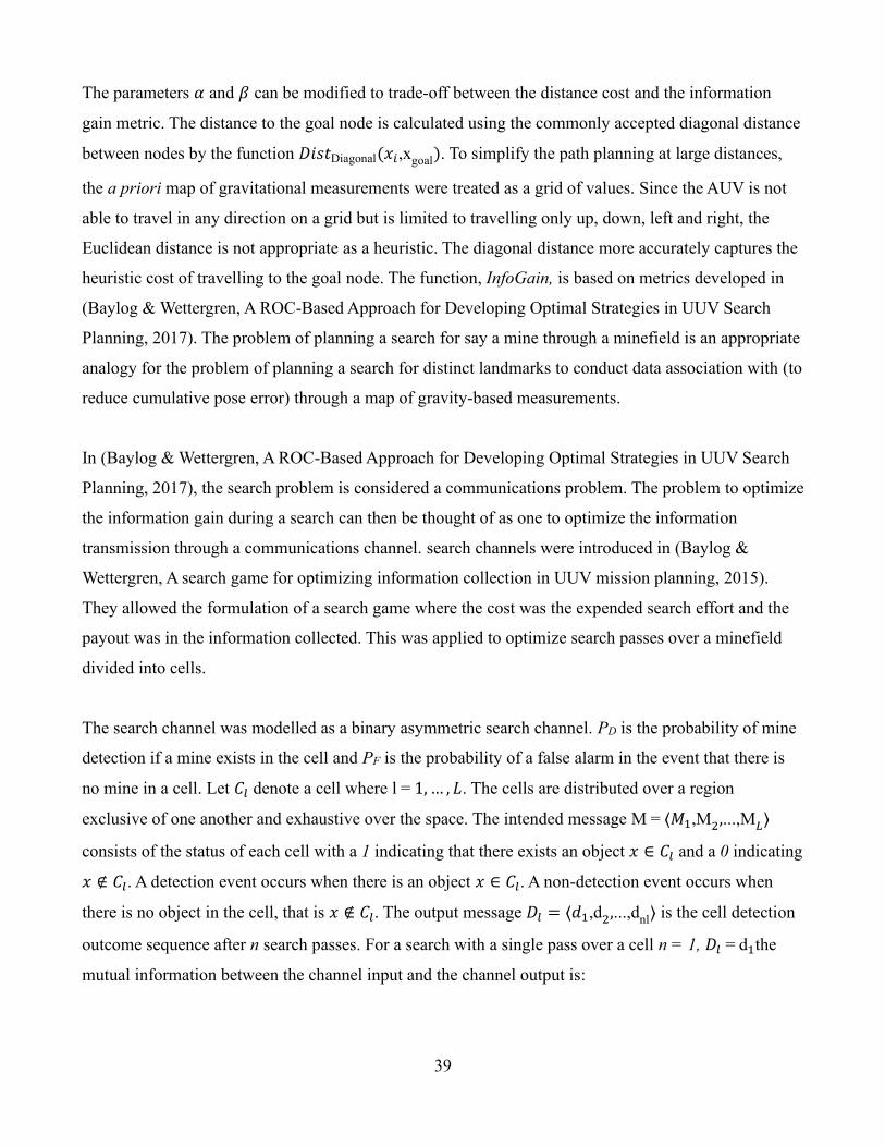
39

The parameters 𝛼 and 𝛽 can be modified to trade-off between the distance cost and the information

gain metric. The distance to the goal node is calculated using the commonly accepted diagonal distance

between nodes by the function 𝐷𝑖𝑠𝑡Diagonal(𝑥𝑖,xgoal). To simplify the path planning at large distances,

the a priori map of gravitational measurements were treated as a grid of values. Since the AUV is not

able to travel in any direction on a grid but is limited to travelling only up, down, left and right, the

Euclidean distance is not appropriate as a heuristic. The diagonal distance more accurately captures the

heuristic cost of travelling to the goal node. The function, InfoGain, is based on metrics developed in

(Baylog & Wettergren, A ROC-Based Approach for Developing Optimal Strategies in UUV Search

Planning, 2017). The problem of planning a search for say a mine through a minefield is an appropriate

analogy for the problem of planning a search for distinct landmarks to conduct data association with (to

reduce cumulative pose error) through a map of gravity-based measurements.

In (Baylog & Wettergren, A ROC-Based Approach for Developing Optimal Strategies in UUV Search

Planning, 2017), the search problem is considered a communications problem. The problem to optimize

the information gain during a search can then be thought of as one to optimize the information

transmission through a communications channel. search channels were introduced in (Baylog &

Wettergren, A search game for optimizing information collection in UUV mission planning, 2015).

They allowed the formulation of a search game where the cost was the expended search effort and the

payout was in the information collected. This was applied to optimize search passes over a minefield

divided into cells.

The search channel was modelled as a binary asymmetric search channel. PD is the probability of mine

detection if a mine exists in the cell and PF is the probability of a false alarm in the event that there is

no mine in a cell. Let 𝐶𝑙 denote a cell where l = 1, … , 𝐿. The cells are distributed over a region

exclusive of one another and exhaustive over the space. The intended message M = ⟨𝑀1,M2,...,M𝐿⟩

consists of the status of each cell with a 1 indicating that there exists an object 𝑥 ∈ 𝐶𝑙 and a 0 indicating

𝑥 ∉ 𝐶𝑙. A detection event occurs when there is an object 𝑥 ∈ 𝐶𝑙. A non-detection event occurs when

there is no object in the cell, that is 𝑥 ∉ 𝐶𝑙. The output message 𝐷𝑙 = ⟨𝑑1,d2,...,dnl⟩ is the cell detection

outcome sequence after n search passes. For a search with a single pass over a cell n = 1, 𝐷𝑙 = d1the

mutual information between the channel input and the channel output is:

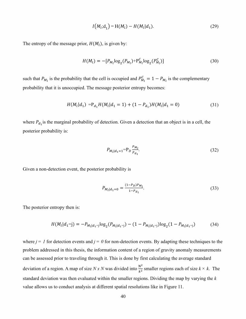
40

𝐼(𝑀𝑙;d1) = H(𝑀𝑙) − 𝐻(𝑀𝑙|𝑑1). (29)

The entropy of the message prior, 𝐻(𝑀𝑙), is given by:

𝐻(𝑀𝑙) = −[𝑃𝑀𝑙log

2(𝑃𝑀𝑙

)+P𝑀𝑙

𝐶 log2

(𝑃𝑀𝑙

𝐶 )] (30)

such that 𝑃𝑀𝑙 is the probability that the cell is occupied and 𝑃𝑀𝑙

𝐶 = 1 − 𝑃𝑀𝑙 is the complementary

probability that it is unoccupied. The message posterior entropy becomes:

𝐻(𝑀𝑙|𝑑1) =P𝑑1𝐻(𝑀𝑙|𝑑1 = 1) + (1 − 𝑃𝑑1

)𝐻(𝑀𝑙|𝑑1 = 0) (31)

where 𝑃𝑑1is the marginal probability of detection. Given a detection that an object is in a cell, the

posterior probability is:

𝑃𝑀𝑙|𝑑1=1=P𝐷

𝑃𝑀𝑙

𝑃𝑑1

. (32)

Given a non-detection event, the posterior probability is

𝑃𝑀𝑙|𝑑1=0 =(1−𝑃𝐷)𝑃𝑀𝑙

1−𝑃𝑑1

. (33)

The posterior entropy then is:

𝐻(𝑀𝑙|𝑑1=j) = −𝑃𝑀𝑙|𝑑1=jlog2

(𝑃𝑀𝑙|𝑑1=j) − (1 − 𝑃𝑀𝑙|𝑑1=j)log2

(1 − 𝑃𝑀𝑙|𝑑1=j) (34)

where j = 1 for detection events and j = 0 for non-detection events. By adapting these techniques to the

problem addressed in this thesis, the information content of a region of gravity anomaly measurements

can be assessed prior to traveling through it. This is done by first calculating the average standard

deviation of a region. A map of size N x N was divided into N2

𝑘2 smaller regions each of size k × k. The

standard deviation was then evaluated within the smaller regions. Dividing the map by varying the k

value allows us to conduct analysis at different spatial resolutions like in Figure 11.

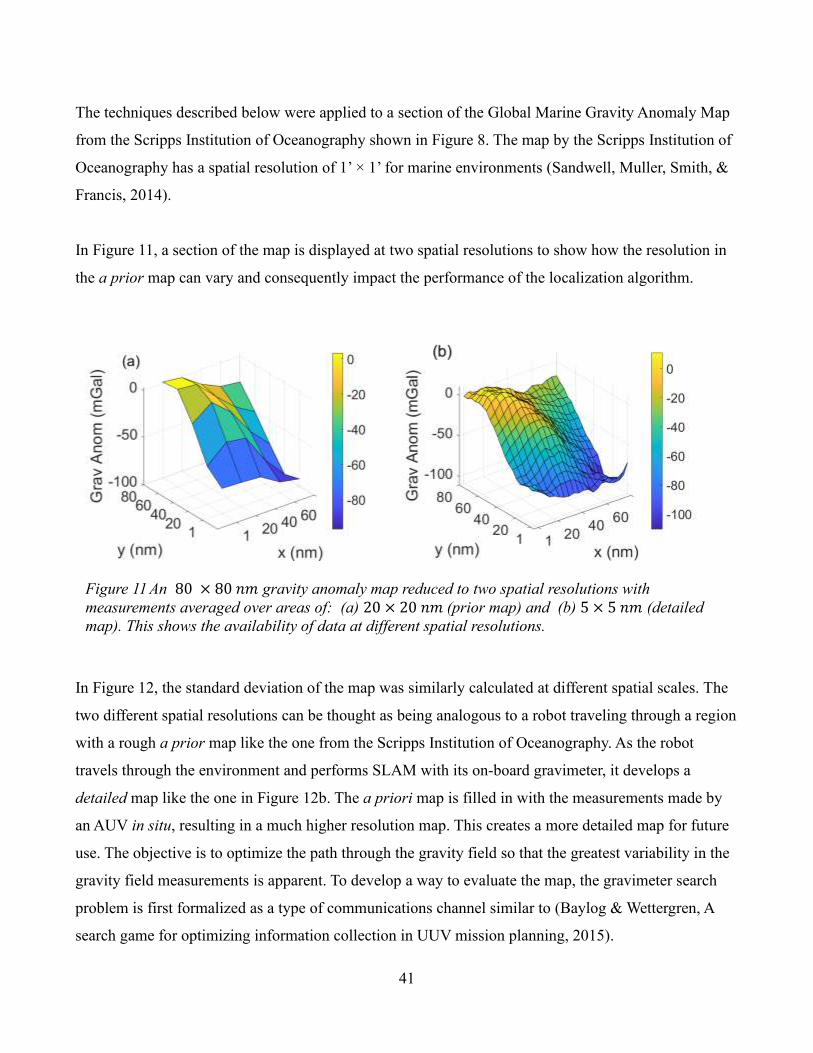
41

The techniques described below were applied to a section of the Global Marine Gravity Anomaly Map

from the Scripps Institution of Oceanography shown in Figure 8. The map by the Scripps Institution of

Oceanography has a spatial resolution of 1’ × 1’ for marine environments (Sandwell, Muller, Smith, &

Francis, 2014).

In Figure 11, a section of the map is displayed at two spatial resolutions to show how the resolution in

the a prior map can vary and consequently impact the performance of the localization algorithm.

In Figure 12, the standard deviation of the map was similarly calculated at different spatial scales. The

two different spatial resolutions can be thought as being analogous to a robot traveling through a region

with a rough a prior map like the one from the Scripps Institution of Oceanography. As the robot

travels through the environment and performs SLAM with its on-board gravimeter, it develops a

detailed map like the one in Figure 12b. The a priori map is filled in with the measurements made by

an AUV in situ, resulting in a much higher resolution map. This creates a more detailed map for future

use. The objective is to optimize the path through the gravity field so that the greatest variability in the

gravity field measurements is apparent. To develop a way to evaluate the map, the gravimeter search

problem is first formalized as a type of communications channel similar to (Baylog & Wettergren, A

search game for optimizing information collection in UUV mission planning, 2015).

Figure 11 An 80 × 80 𝑛𝑚 gravity anomaly map reduced to two spatial resolutions with

measurements averaged over areas of: (a) 20 × 20 𝑛𝑚 (prior map) and (b) 5 × 5 𝑛𝑚 (detailed

map). This shows the availability of data at different spatial resolutions.

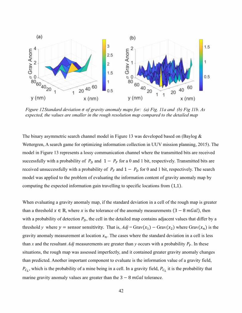
42

The binary asymmetric search channel model in Figure 13 was developed based on (Baylog &

Wettergren, A search game for optimizing information collection in UUV mission planning, 2015). The

model in Figure 13 represents a lossy communication channel where the transmitted bits are received

successfully with a probability of 𝑃𝐷 and 1 − 𝑃𝐹 for a 0 and 1 bit, respectively. Transmitted bits are

received unsuccessfully with a probability of 𝑃𝐹 and 1 − 𝑃𝐷 for 0 and 1 bit, respectively. The search

model was applied to the problem of evaluating the information content of gravity anomaly map by

computing the expected information gain travelling to specific locations from (1,1).

When evaluating a gravity anomaly map, if the standard deviation in a cell of the rough map is greater

than a threshold 𝑥 ∈ ℝ, where 𝑥 is the tolerance of the anomaly measurements (3 − 8 𝑚𝐺𝑎𝑙), then

with a probability of detection 𝑃𝐷, the cell in the detailed map contains adjacent values that differ by a

threshold y where 𝑦 = sensor sensitivity. That is, Adj = Grav(𝑥1) − Grav(𝑥2) where Grav(𝑥𝑛) is the

gravity anomaly measurement at location 𝑥𝑛. The cases where the standard deviation in a cell is less

than x and the resultant Adj measurements are greater than y occurs with a probability 𝑃𝐹. In these

situations, the rough map was assessed imperfectly, and it contained greater gravity anomaly changes

than predicted. Another important component to evaluate is the information value of a gravity field,

𝑃𝐶𝐿, which is the probability of a mine being in a cell. In a gravity field, 𝑃𝐶𝐿

it is the probability that

marine gravity anomaly values are greater than the 3 − 8 𝑚𝐺𝑎𝑙 tolerance.

Figure 12 Standard deviation 𝜎 of gravity anomaly maps for: (a) Fig. 11a and (b) Fig 11b. As

expected, the values are smaller in the rough resolution map compared to the detailed map

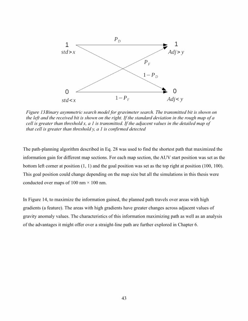
43

The path-planning algorithm described in Eq. 28 was used to find the shortest path that maximized the

information gain for different map sections. For each map section, the AUV start position was set as the

bottom left corner at position (1, 1) and the goal position was set as the top right at position (100, 100).

This goal position could change depending on the map size but all the simulations in this thesis were

conducted over maps of 100 nm × 100 nm.

In Figure 14, to maximize the information gained, the planned path travels over areas with high

gradients (a feature). The areas with high gradients have greater changes across adjacent values of

gravity anomaly values. The characteristics of this information maximizing path as well as an analysis

of the advantages it might offer over a straight-line path are further explored in Chapter 6.

Figure 13 Binary asymmetric search model for gravimeter search. The transmitted bit is shown on

the left and the received bit is shown on the right. If the standard deviation in the rough map of a

cell is greater than threshold x, a 1 is transmitted. If the adjacent values in the detailed map of

that cell is greater than threshold y, a 1 is confirmed detected

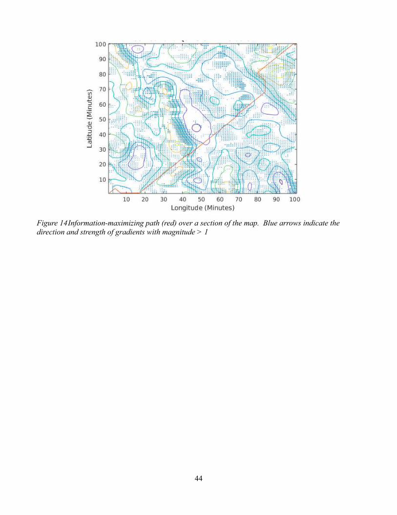
44

Figure 14 Information-maximizing path (red) over a section of the map. Blue arrows indicate the

direction and strength of gradients with magnitude > 1

45

5.3 RBPF SLAM

Section 5.1 Particle Filter-Based Localization and Mapping described the developed particle filter-

based localization algorithm using an a priori map. To implement a localization algorithm without an a

priori map, a SLAM system was developed. For implementation of the proposed gravity-based SLAM

system, the FastSLAM algorithm was chosen. FastSLAM is a particle filter-based solution for the

SLAM problem (Montemerlo, Thrun, Koller, & Wegbreit, 2002). As mentioned earlier, it is a non-

parametric implementation of a Bayes filter where the posterior is represented by a set of weighted

samples (particles). As stated previously, a particle filter-based implementation has a number of

advantages over an EKF-based implementation that makes it suitable to the problem. The most

important advantage is that it is possible to have a nonlinear measurement model h, which is a more

general solution than the linear Kalman filter. This is an important property for the gravity-based

measurement system since it allows one to obtain an estimate of the robot position from a gravity

measurement. Another important property of particle filter-based algorithms is that they can capture

multimodal distributions, which allows the representation of situations where the particle filter

diverges due to multiple similar paths through the gravity field that would lead to similar observations.

An EKF would be unable to model such a situation and would quickly break down, while a particle

filter-based system can support multiple hypotheses and collapses to the correct one once loop closure

occurs. Another consideration was the efficiency of the algorithm. Due to the long ranges that were

being simulated, an inefficient algorithm would task the embedded processor on AUVs. FastSLAM

was designed to be, as the name implies, fast. All these advantages made FastSLAM the most suitable

choice for the purposes of this thesis. Additionally, a particle filter-based SLAM algorithm is a natural

extension of the particle filter-based localization algorithm previously developed, thus allowing for

quicker implementation. The key difference being that a particle filter-based SLAM system would

operate without the use of an a priori map.

The steps of a particle filter-based SLAM system remain the same as the particle filter-based

localization and navigation system. There is a three-step procedure consisting of sampling from the

proposal distribution, computing the importance weights, and then resampling (Stachniss, 2013). The

key idea behind FastSLAM is the Rao-Blackwellization of the SLAM posterior. The RBPF performs a

marginalization of the probability distribution of the state space by factorizing the SLAM posterior.

p(a, b) = 𝑝(𝑏|𝑎)𝑝(𝑎) (35)

46

Consider the above case where the objective is to compute the joint probability distribution of 𝑎 and 𝑏

p (a, b). If p(b | a) were computed efficiently, then p(a) should be represented with samples and then

p(b | a) would be computed for every sample. Now, consider the SLAM problem. In SLAM, the aim is

to compute the following probability distribution:

p(x0:t, m1:M|z1:t, u1:t). (36)

The above probability distribution describes the likely pose of the robot x0:t and the environment

m1:M. It can be factorized as follows:

p(x0:t, m1:M|z1:t, u1:t) = p(x0:t|𝑧1;𝑡, 𝑢1:𝑡)𝑝(𝑚1:𝑀|𝑥0:𝑡, 𝑧1:𝑡). (37)

The question then becomes how to compute 𝑝(𝑚1:𝑀|𝑥0:𝑡, 𝑧1:𝑡) efficiently. RBPF accomplishes this by

representing them as multiple two-dimensional EKFs. Equation 37 therefore becomes:

p(x0:t, m1:M|z1:t, u1:t) = p(x0:t|𝑧1;𝑡, 𝑢1:𝑡) ∏ 𝑝(𝑚𝑖|𝑥0:𝑡, 𝑧1:𝑡)𝑀𝑖=1 . (38)

Each particle is a path hypothesis and represents p(x0:t|𝑧1;𝑡, 𝑢1:𝑡). The challenge now is in computing

the importance weight 𝑤[𝑘] of each sample. In FastSLAM, the importance weight is approximated as

follows:

w[𝑘] = |2𝜋𝑄|−1

2 exp {−1

2(𝑧𝑡 − �̂�[𝑘])

𝑇𝑄−1(𝑧𝑡 − �̂�[𝑘])}. (39)

After computing the importance weight of each particle, the set of particles are resampled with

replacement. After resampling, the particle distribution better represents the estimated view of the

world. That is, they represent hypotheses of the robot poses, the robot’s pose history, and a map of the

landmarks in the environment. The full FastSLAM algorithm is not described here due to its similarity

to particle filter localization. Further details may be found in (Thrun, Burgard, & Fox, 2005),

(Montemerlo, Thrun, Koller, & Wegbreit, 2002), and (Stachniss, 2013).

47

To predict a hypothesis and achieve SLAM without an a priori map the predicted observation �̂�[𝑘] was

calculated as follows:

�̂�𝑡𝑘 = 𝑧𝑡−1

𝑘 . (40)

The key idea is that the next observation is not expected to differ significantly from the last

observation. While more sophisticated methods to compute the predicted observation exists, for

simulation purposes, Eq. 40 was deemed sufficient. Unlike SLAM implemented using traditional

sensors, it is not possible to compute the predicted observation from a predicted pose. This is because a

measurement of the gravity anomaly gives no information about the relative pose of the robot

compared to a landmark. The measurement also does not give any information about the absolute pose

of the robot without an a priori map. This is an area which could benefit from further research and

development of more informed predictions. Prediction and inference of data is an active area of

considerable research (Zeyu & Srinivasan, 2017) (Saxena, Sun, & Ng, 2009). Techniques from AI

research could be applied to develop a better performing gravity-based SLAM algorithm. For the

current implementation, ideas from the emerging field of heuristic decision-making were borrowed

(Gigerenzer & Gaissmaier, 2011) which indicate that simple heuristics used in an adaptive way can

lead to more accurate judgements than weighing and adding all information. This can be an effective

technique in instances of low predictability and small samples. While this was not a perfect analogy to

the problem of predicting a gravity anomaly measurement, it is similar, and shares the same concerns

with overfitting to historical data. Further work in this area was left for future work and is outside of

the scope of this thesis.

Data association is a fundamental component of the SLAM problem. Data association is the process of

correctly identifying features in the environment and correctly associating them as features that were

previously observed (visited). There are FastSLAM implementations that perform data association

between features using scan matching or, as in this situation, conduct data association tests between

landmarks in the environment. Scan matching is a technique best employed when the sensor used by

the robot produces a large amount of data at each time step. The objective of scan matching is to

compute the maximum likely alignment between two sets of raw sensor data, allowing for data

association to be performed using multiple measurements (Nieto, Bailey, & Nebot, 2007).

48

For the simulation purpose here, the gravity data was treated as individual landmarks. This is due to the

sparseness of the available gravity dataset, which only have measurements every 1 nm. In a practical

implementation of a gravity-based SLAM system, it is recommended that a scan matching-type system

be implemented similar to that of (Quintas, Teixeira, & Pascoal, 2018).

Given a measurement 𝑧𝑡, the purpose of data association is to generate a hypothesis 𝐻 = {𝑗} that

matches a map feature in the map 𝑚𝑀 = {𝑘1, 𝑘2, … , 𝑘𝑀}. When previously visited landmarks are

revisited and correctly associated, loop closure can be conducted to reduce the robot’s position

uncertainty. A number of different data association techniques have been developed like joint

compatibility branch and bound (JCBB) (Neira & Tardós, 2001) and lazy data association (Hahnel,

Thrun, Wegbreit, & Burgard, 2005). In this thesis, a simple approach similar to nearest neighbor was

implemented. The AUV compares the current measurements zt to the previous measurements at the

same location. If the measurements match, then the same landmark was re-observed and consequently,

the covariance, as well as the estimated landmark position, is updated. The simplicity of the chosen

data association algorithm made it easier to test the impact of the proposed “SLAMability” metric.

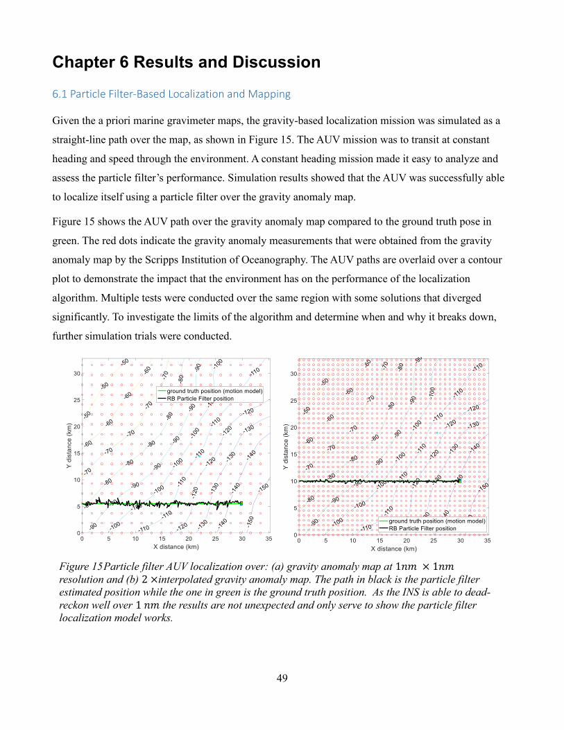
49

Chapter 6 Results and Discussion

6.1 Particle Filter-Based Localization and Mapping

Given the a priori marine gravimeter maps, the gravity-based localization mission was simulated as a

straight-line path over the map, as shown in Figure 15. The AUV mission was to transit at constant

heading and speed through the environment. A constant heading mission made it easy to analyze and

assess the particle filter’s performance. Simulation results showed that the AUV was successfully able

to localize itself using a particle filter over the gravity anomaly map.

Figure 15 shows the AUV path over the gravity anomaly map compared to the ground truth pose in

green. The red dots indicate the gravity anomaly measurements that were obtained from the gravity

anomaly map by the Scripps Institution of Oceanography. The AUV paths are overlaid over a contour

plot to demonstrate the impact that the environment has on the performance of the localization

algorithm. Multiple tests were conducted over the same region with some solutions that diverged

significantly. To investigate the limits of the algorithm and determine when and why it breaks down,

further simulation trials were conducted.

Figure 15 Particle filter AUV localization over: (a) gravity anomaly map at 1𝑛𝑚 × 1𝑛𝑚

resolution and (b) 2 ×interpolated gravity anomaly map. The path in black is the particle filter

estimated position while the one in green is the ground truth position. As the INS is able to dead-

reckon well over 1 𝑛𝑚 the results are not unexpected and only serve to show the particle filter

localization model works.

50

Figure 15(b) shows the same AUV path simulated over an interpolated map of gravity anomaly

measurements. The interpolated map was calculated using the Mathworks MATLAB linear

interpolation function. The results over multiple trials showed that there was no significant difference

in the performance of the interpolated map compared to the original gravity anomaly map. A possible

reason for this might be that while the AUV was able to conduct more frequent gravity-based

measurements with the interpolated map, the distinctness of the measurements was reduced. This was

because the gradient of adjacent measurements was now smaller in magnitude due to the distances

between them being reduced.

Results from additional simulation trials are shown in Figure 16. The number of particles in the particle

filter was varied from 40 to 200. Figure 16 shows the performance of the particle filter algorithm in red

compared to the performance of an INS that accumulated an error of 1% of the distance travelled

(state-of-the-art). On the top left is the mean error in the x direction in kilometers, the top right is the

mean error in the y direction, the bottom left is the standard deviation of the error in the x direction in

kilometers and the bottom right is the standard deviation of the error in the y direction. The mean error

was calculated by averaging the error of the final AUV position at the end of the simulation run shown

in. The particle filter-based algorithm clearly has superior localization performance. That is, the

average localization error of the particle filter when compared to the ground truth position is observed

to be generally lower than the average error with the INS solution. It is also observed that the

localization error decreases as the number of particles used in the particle filter increases, with a sharp

decline initially and then gradually reaching a point of diminishing returns. This is not unexpected for

particle filters. The mean error of the localization performance in the y direction, shown in the top right

of Figure 16, indicates that there is poor performance along one direction. This could have been due to

the map over which the simulation was conducted. From the map contours of Figure 15, it appears that

the gravity anomaly measurements change more steeply along the x direction than the y direction. To

investigate how the map type impacts the localization algorithm performance, simulations were

conducted over different map sections.

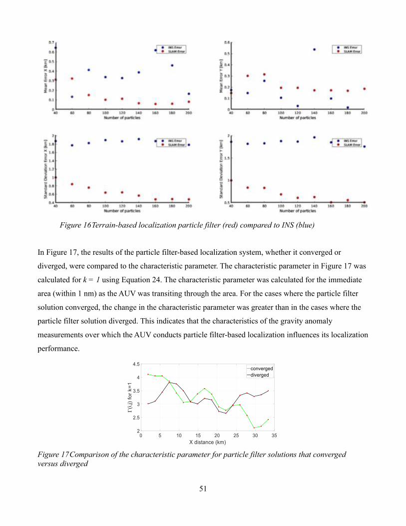
51

In Figure 17, the results of the particle filter-based localization system, whether it converged or

diverged, were compared to the characteristic parameter. The characteristic parameter in Figure 17 was

calculated for k = 1 using Equation 24. The characteristic parameter was calculated for the immediate

area (within 1 nm) as the AUV was transiting through the area. For the cases where the particle filter

solution converged, the change in the characteristic parameter was greater than in the cases where the

particle filter solution diverged. This indicates that the characteristics of the gravity anomaly

measurements over which the AUV conducts particle filter-based localization influences its localization

performance.

Figure 17 Comparison of the characteristic parameter for particle filter solutions that converged

versus diverged

Figure 16 Terrain-based localization particle filter (red) compared to INS (blue)

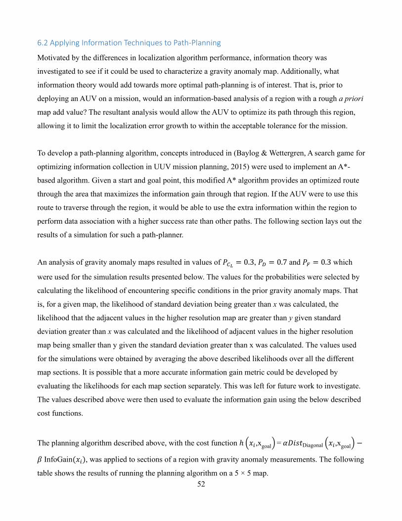
52

6.2 Applying Information Techniques to Path-Planning

Motivated by the differences in localization algorithm performance, information theory was

investigated to see if it could be used to characterize a gravity anomaly map. Additionally, what

information theory would add towards more optimal path-planning is of interest. That is, prior to

deploying an AUV on a mission, would an information-based analysis of a region with a rough a priori

map add value? The resultant analysis would allow the AUV to optimize its path through this region,

allowing it to limit the localization error growth to within the acceptable tolerance for the mission.

To develop a path-planning algorithm, concepts introduced in (Baylog & Wettergren, A search game for

optimizing information collection in UUV mission planning, 2015) were used to implement an A*-

based algorithm. Given a start and goal point, this modified A* algorithm provides an optimized route

through the area that maximizes the information gain through that region. If the AUV were to use this

route to traverse through the region, it would be able to use the extra information within the region to

perform data association with a higher success rate than other paths. The following section lays out the

results of a simulation for such a path-planner.

An analysis of gravity anomaly maps resulted in values of 𝑃𝐶𝐿= 0.3, 𝑃𝐷 = 0.7 and 𝑃𝐹 = 0.3 which

were used for the simulation results presented below. The values for the probabilities were selected by

calculating the likelihood of encountering specific conditions in the prior gravity anomaly maps. That

is, for a given map, the likelihood of standard deviation being greater than x was calculated, the

likelihood that the adjacent values in the higher resolution map are greater than y given standard

deviation greater than x was calculated and the likelihood of adjacent values in the higher resolution

map being smaller than y given the standard deviation greater than x was calculated. The values used

for the simulations were obtained by averaging the above described likelihoods over all the different

map sections. It is possible that a more accurate information gain metric could be developed by

evaluating the likelihoods for each map section separately. This was left for future work to investigate.

The values described above were then used to evaluate the information gain using the below described

cost functions.

The planning algorithm described above, with the cost function ℎ (𝑥𝑖,xgoal) = 𝛼𝐷𝑖𝑠𝑡Diagonal (𝑥𝑖,xgoal) −

𝛽 InfoGain(𝑥𝑖), was applied to sections of a region with gravity anomaly measurements. The following

table shows the results of running the planning algorithm on a 5 × 5 map.

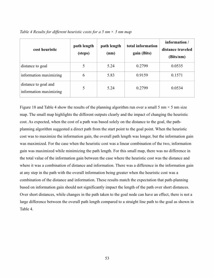
53

Table 4 Results for different heuristic costs for a 5 nm × 5 nm map

cost heuristic path length

(steps)

path length

(nm)

total information

gain (Bits)

information /

distance traveled

(Bits/nm)

distance to goal 5 5.24 0.2799 0.0535

information maximizing 6 5.83 0.9159 0.1571

distance to goal and

information maximizing 5 5.24 0.2799 0.0534

Figure 18 and Table 4 show the results of the planning algorithm run over a small 5 nm × 5 nm size

map. The small map highlights the different outputs clearly and the impact of changing the heuristic

cost. As expected, when the cost of a path was based solely on the distance to the goal, the path-

planning algorithm suggested a direct path from the start point to the goal point. When the heuristic

cost was to maximize the information gain, the overall path length was longer, but the information gain

was maximized. For the case when the heuristic cost was a linear combination of the two, information

gain was maximized while minimizing the path length. For this small map, there was no difference in

the total value of the information gain between the case where the heuristic cost was the distance and

where it was a combination of distance and information. There was a difference in the information gain

at any step in the path with the overall information being greater when the heuristic cost was a

combination of the distance and information. These results match the expectation that path-planning

based on information gain should not significantly impact the length of the path over short distances.

Over short distances, while changes in the path taken to the goal node can have an effect, there is not a

large difference between the overall path length compared to a straight line path to the goal as shown in

Table 4.

54

The same path planning algorithm was applied to a 40 × 40 map. The results are depicted in Table 5

and Figure 19.

Table 5 Results for different heuristic costs for a 40 nm × 40 nm map

cost heuristic path length

(steps)

path length

(nm)

total information

gain (Bits)

information /

distance traveled

(Bits/nm)

distance to goal 40 55.15 7.0687 0.1282

information maximizing 44 57.50 10.7449 0.1869

distance to goal and

information maximizing 42 55.15 9.4728 0.1718

For a larger map size of 40 × 40, the trade-off between information gain and distance to the goal is

more significant over the longer distance. As expected, when the heuristic cost was only based on the

Figure 18 Path through gravity field that maximizes the heuristic, (a) Distance, (b) Information,

(c) Distance and Information for a 5 × 5 map. Note, that the information gain metric has the

largest change in the path taken to reach the goal node.

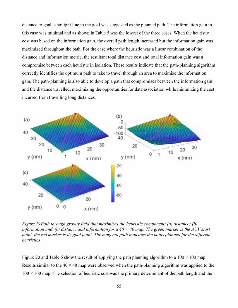
55

distance to goal, a straight line to the goal was suggested as the planned path. The information gain in

this case was minimal and as shown in Table 5 was the lowest of the three cases. When the heuristic

cost was based on the information gain, the overall path length increased but the information gain was

maximized throughout the path. For the case where the heuristic was a linear combination of the

distance and information metric, the resultant total distance cost and total information gain was a

compromise between each heuristic in isolation. These results indicate that the path-planning algorithm

correctly identifies the optimum path to take to travel through an area to maximize the information

gain. The path-planning is also able to develop a path that compromises between the information gain

and the distance travelled, maximizing the opportunities for data association while minimizing the cost

incurred from travelling long distances.

Figure 20 and Table 6 show the result of applying the path planning algorithm to a 100 × 100 map.

Results similar to the 40 × 40 map were observed when the path-planning algorithm was applied to the

100 × 100 map. The selection of heuristic cost was the primary determinant of the path length and the

Figure 19 Path through gravity field that maximizes the heuristic component: (a) distance; (b)

information and (c) distance and information for a 40 × 40 map. The green marker is the AUV start

point, the red marker is its goal point. The magenta path indicates the paths planned for the different

heuristics

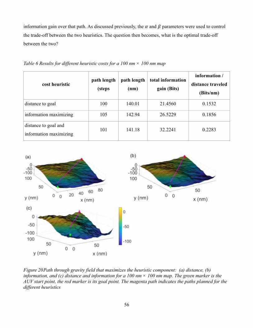
56

information gain over that path. As discussed previously, the 𝛼 and 𝛽 parameters were used to control

the trade-off between the two heuristics. The question then becomes, what is the optimal trade-off

between the two?

Table 6 Results for different heuristic costs for a 100 nm × 100 nm map

cost heuristic path length

(steps

path length

(nm)

total information

gain (Bits)

information /

distance traveled

(Bits/nm)

distance to goal 100 140.01 21.4560 0.1532

information maximizing 105 142.94 26.5229 0.1856

distance to goal and

information maximizing 101 141.18 32.2241 0.2283

Figure 20 Path through gravity field that maximizes the heuristic component: (a) distance, (b)

information, and (c) distance and information for a 100 nm × 100 nm map. The green marker is the

AUV start point, the red marker is its goal point. The magenta path indicates the paths planned for the

different heuristics

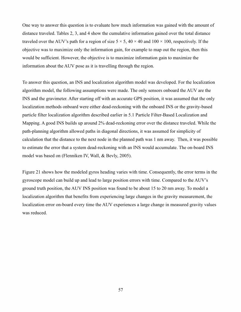
57

One way to answer this question is to evaluate how much information was gained with the amount of

distance traveled. Tables 2, 3, and 4 show the cumulative information gained over the total distance

traveled over the AUV’s path for a region of size 5 × 5, 40 × 40 and 100 × 100, respectively. If the

objective was to maximize only the information gain, for example to map out the region, then this

would be sufficient. However, the objective is to maximize information gain to maximize the

information about the AUV pose as it is travelling through the region.

To answer this question, an INS and localization algorithm model was developed. For the localization

algorithm model, the following assumptions were made. The only sensors onboard the AUV are the

INS and the gravimeter. After starting off with an accurate GPS position, it was assumed that the only

localization methods onboard were either dead-reckoning with the onboard INS or the gravity-based

particle filter localization algorithm described earlier in 5.1 Particle Filter-Based Localization and

Mapping. A good INS builds up around 2% dead-reckoning error over the distance traveled. While the

path-planning algorithm allowed paths in diagonal directions, it was assumed for simplicity of

calculation that the distance to the next node in the planned path was 1 nm away. Then, it was possible

to estimate the error that a system dead-reckoning with an INS would accumulate. The on-board INS

model was based on (Flenniken IV, Wall, & Bevly, 2005).

Figure 21 shows how the modeled gyros heading varies with time. Consequently, the error terms in the

gyroscope model can build up and lead to large position errors with time. Compared to the AUV’s

ground truth position, the AUV INS position was found to be about 15 to 20 nm away. To model a

localization algorithm that benefits from experiencing large changes in the gravity measurement, the

localization error on-board every time the AUV experiences a large change in measured gravity values

was reduced.

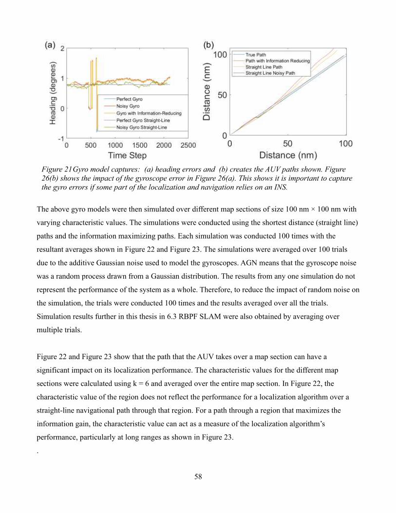
58

The above gyro models were then simulated over different map sections of size 100 nm × 100 nm with

varying characteristic values. The simulations were conducted using the shortest distance (straight line)

paths and the information maximizing paths. Each simulation was conducted 100 times with the

resultant averages shown in Figure 22 and Figure 23. The simulations were averaged over 100 trials

due to the additive Gaussian noise used to model the gyroscopes. AGN means that the gyroscope noise

was a random process drawn from a Gaussian distribution. The results from any one simulation do not

represent the performance of the system as a whole. Therefore, to reduce the impact of random noise on

the simulation, the trials were conducted 100 times and the results averaged over all the trials.

Simulation results further in this thesis in 6.3 RBPF SLAM were also obtained by averaging over

multiple trials.

Figure 22 and Figure 23 show that the path that the AUV takes over a map section can have a

significant impact on its localization performance. The characteristic values for the different map

sections were calculated using k = 6 and averaged over the entire map section. In Figure 22, the

characteristic value of the region does not reflect the performance for a localization algorithm over a

straight-line navigational path through that region. For a path through a region that maximizes the

information gain, the characteristic value can act as a measure of the localization algorithm’s

performance, particularly at long ranges as shown in Figure 23.

.

Figure 21 Gyro model captures: (a) heading errors and (b) creates the AUV paths shown. Figure

26(b) shows the impact of the gyroscope error in Figure 26(a). This shows it is important to capture

the gyro errors if some part of the localization and navigation relies on an INS.

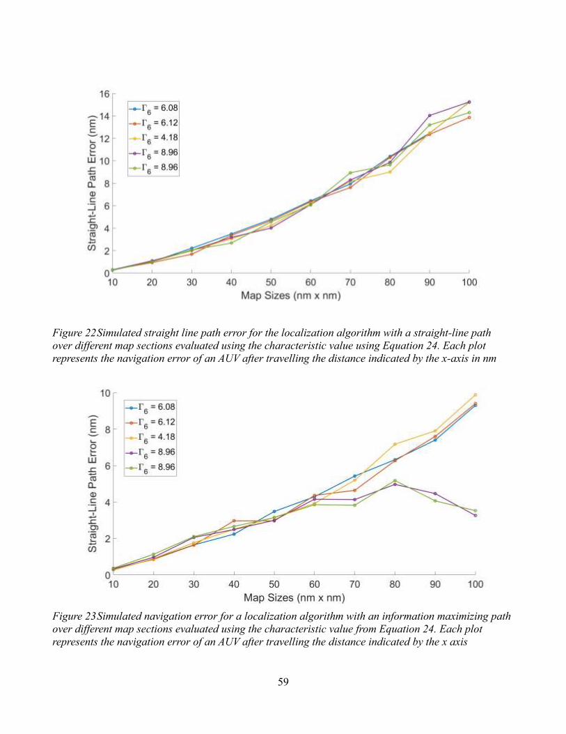
59

Figure 23 Simulated navigation error for a localization algorithm with an information maximizing path

over different map sections evaluated using the characteristic value from Equation 24. Each plot

represents the navigation error of an AUV after travelling the distance indicated by the x axis

Figure 22 Simulated straight line path error for the localization algorithm with a straight-line path

over different map sections evaluated using the characteristic value using Equation 24. Each plot

represents the navigation error of an AUV after travelling the distance indicated by the x-axis in nm

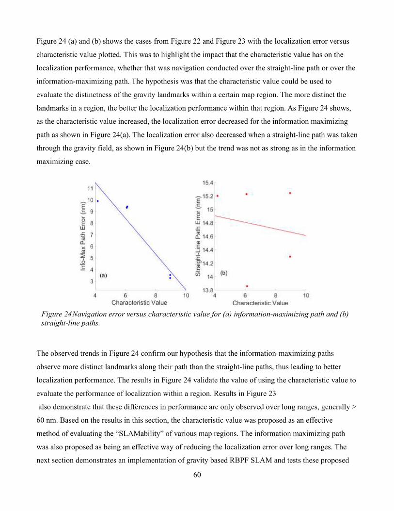
60

Figure 24 (a) and (b) shows the cases from Figure 22 and Figure 23 with the localization error versus

characteristic value plotted. This was to highlight the impact that the characteristic value has on the

localization performance, whether that was navigation conducted over the straight-line path or over the

information-maximizing path. The hypothesis was that the characteristic value could be used to

evaluate the distinctness of the gravity landmarks within a certain map region. The more distinct the

landmarks in a region, the better the localization performance within that region. As Figure 24 shows,

as the characteristic value increased, the localization error decreased for the information maximizing

path as shown in Figure 24(a). The localization error also decreased when a straight-line path was taken

through the gravity field, as shown in Figure 24(b) but the trend was not as strong as in the information

maximizing case.

The observed trends in Figure 24 confirm our hypothesis that the information-maximizing paths

observe more distinct landmarks along their path than the straight-line paths, thus leading to better

localization performance. The results in Figure 24 validate the value of using the characteristic value to

evaluate the performance of localization within a region. Results in Figure 23

also demonstrate that these differences in performance are only observed over long ranges, generally >

60 nm. Based on the results in this section, the characteristic value was proposed as an effective

method of evaluating the “SLAMability” of various map regions. The information maximizing path

was also proposed as being an effective way of reducing the localization error over long ranges. The

next section demonstrates an implementation of gravity based RBPF SLAM and tests these proposed

Figure 24 Navigation error versus characteristic value for (a) information-maximizing path and (b)

straight-line paths.

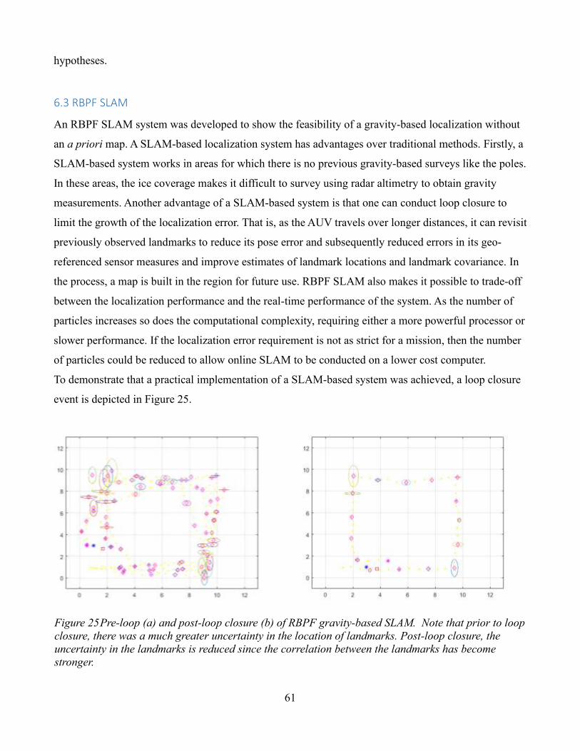
61

hypotheses.

6.3 RBPF SLAM

An RBPF SLAM system was developed to show the feasibility of a gravity-based localization without

an a priori map. A SLAM-based localization system has advantages over traditional methods. Firstly, a

SLAM-based system works in areas for which there is no previous gravity-based surveys like the poles.

In these areas, the ice coverage makes it difficult to survey using radar altimetry to obtain gravity

measurements. Another advantage of a SLAM-based system is that one can conduct loop closure to

limit the growth of the localization error. That is, as the AUV travels over longer distances, it can revisit

previously observed landmarks to reduce its pose error and subsequently reduced errors in its geo-

referenced sensor measures and improve estimates of landmark locations and landmark covariance. In

the process, a map is built in the region for future use. RBPF SLAM also makes it possible to trade-off

between the localization performance and the real-time performance of the system. As the number of

particles increases so does the computational complexity, requiring either a more powerful processor or

slower performance. If the localization error requirement is not as strict for a mission, then the number

of particles could be reduced to allow online SLAM to be conducted on a lower cost computer.

To demonstrate that a practical implementation of a SLAM-based system was achieved, a loop closure

event is depicted in Figure 25.

Figure 25 Pre-loop (a) and post-loop closure (b) of RBPF gravity-based SLAM. Note that prior to loop

closure, there was a much greater uncertainty in the location of landmarks. Post-loop closure, the

uncertainty in the landmarks is reduced since the correlation between the landmarks has become

stronger.

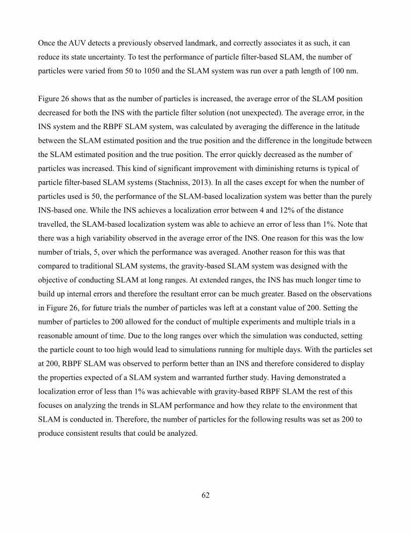
62

Once the AUV detects a previously observed landmark, and correctly associates it as such, it can

reduce its state uncertainty. To test the performance of particle filter-based SLAM, the number of

particles were varied from 50 to 1050 and the SLAM system was run over a path length of 100 nm.

Figure 26 shows that as the number of particles is increased, the average error of the SLAM position

decreased for both the INS with the particle filter solution (not unexpected). The average error, in the

INS system and the RBPF SLAM system, was calculated by averaging the difference in the latitude

between the SLAM estimated position and the true position and the difference in the longitude between

the SLAM estimated position and the true position. The error quickly decreased as the number of

particles was increased. This kind of significant improvement with diminishing returns is typical of

particle filter-based SLAM systems (Stachniss, 2013). In all the cases except for when the number of

particles used is 50, the performance of the SLAM-based localization system was better than the purely

INS-based one. While the INS achieves a localization error between 4 and 12% of the distance

travelled, the SLAM-based localization system was able to achieve an error of less than 1%. Note that

there was a high variability observed in the average error of the INS. One reason for this was the low

number of trials, 5, over which the performance was averaged. Another reason for this was that

compared to traditional SLAM systems, the gravity-based SLAM system was designed with the

objective of conducting SLAM at long ranges. At extended ranges, the INS has much longer time to

build up internal errors and therefore the resultant error can be much greater. Based on the observations

in Figure 26, for future trials the number of particles was left at a constant value of 200. Setting the

number of particles to 200 allowed for the conduct of multiple experiments and multiple trials in a

reasonable amount of time. Due to the long ranges over which the simulation was conducted, setting

the particle count to too high would lead to simulations running for multiple days. With the particles set

at 200, RBPF SLAM was observed to perform better than an INS and therefore considered to display

the properties expected of a SLAM system and warranted further study. Having demonstrated a

localization error of less than 1% was achievable with gravity-based RBPF SLAM the rest of this

focuses on analyzing the trends in SLAM performance and how they relate to the environment that

SLAM is conducted in. Therefore, the number of particles for the following results was set as 200 to

produce consistent results that could be analyzed.

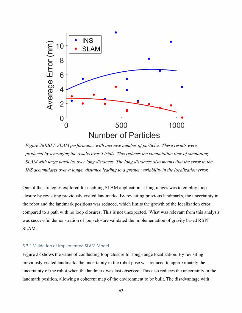
63

One of the strategies explored for enabling SLAM application at long ranges was to employ loop

closure by revisiting previously visited landmarks. By revisiting previous landmarks, the uncertainty in

the robot and the landmark positions was reduced, which limits the growth of the localization error

compared to a path with no loop closures. This is not unexpected. What was relevant from this analysis

was successful demonstration of loop closure validated the implementation of gravity based RBPF

SLAM.

6.3.1 Validation of Implemented SLAM Model

Figure 28 shows the value of conducting loop closure for long-range localization. By revisiting

previously visited landmarks the uncertainty in the robot pose was reduced to approximately the

uncertainty of the robot when the landmark was last observed. This also reduces the uncertainty in the

landmark position, allowing a coherent map of the environment to be built. The disadvantage with

Figure 26 RBPF SLAM performance with increase number of particles. These results were

produced by averaging the results over 5 trials. This reduces the computation time of simulating

SLAM with large particles over long distances. The long distances also means that the error in the

INS accumulates over a longer distance leading to a greater variability in the localization error.

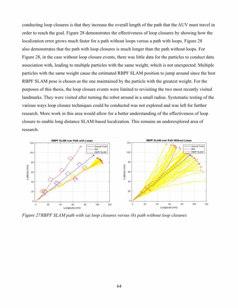
64

conducting loop closures is that they increase the overall length of the path that the AUV must travel in

order to reach the goal. Figure 28 demonstrates the effectiveness of loop closures by showing how the

localization error grows much faster for a path without loops versus a path with loops. Figure 28

also demonstrates that the path with loop closures is much longer than the path without loops. For

Figure 28, in the case without loop closure events, there was little data for the particles to conduct data

association with, leading to multiple particles with the same weight, which is not unexpected. Multiple

particles with the same weight cause the estimated RBPF SLAM position to jump around since the best

RBPF SLAM pose is chosen as the one maintained by the particle with the greatest weight. For the

purposes of this thesis, the loop closure events were limited to revisiting the two most recently visited

landmarks. They were visited after turning the robot around in a small radius. Systematic testing of the

various ways loop closure techniques could be conducted was not explored and was left for further

research. More work in this area would allow for a better understanding of the effectiveness of loop

closure to enable long distance SLAM-based localization. This remains an underexplored area of

research.

Figure 27 RBPF SLAM path with (a) loop closures versus (b) path without loop closures

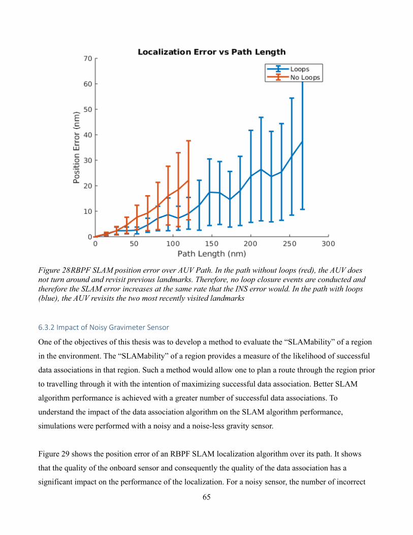
65

6.3.2 Impact of Noisy Gravimeter Sensor

One of the objectives of this thesis was to develop a method to evaluate the “SLAMability” of a region

in the environment. The “SLAMability” of a region provides a measure of the likelihood of successful

data associations in that region. Such a method would allow one to plan a route through the region prior

to travelling through it with the intention of maximizing successful data association. Better SLAM

algorithm performance is achieved with a greater number of successful data associations. To

understand the impact of the data association algorithm on the SLAM algorithm performance,

simulations were performed with a noisy and a noise-less gravity sensor.

Figure 29 shows the position error of an RBPF SLAM localization algorithm over its path. It shows

that the quality of the onboard sensor and consequently the quality of the data association has a

significant impact on the performance of the localization. For a noisy sensor, the number of incorrect

Figure 28 RBPF SLAM position error over AUV Path. In the path without loops (red), the AUV does

not turn around and revisit previous landmarks. Therefore, no loop closure events are conducted and

therefore the SLAM error increases at the same rate that the INS error would. In the path with loops

(blue), the AUV revisits the two most recently visited landmarks

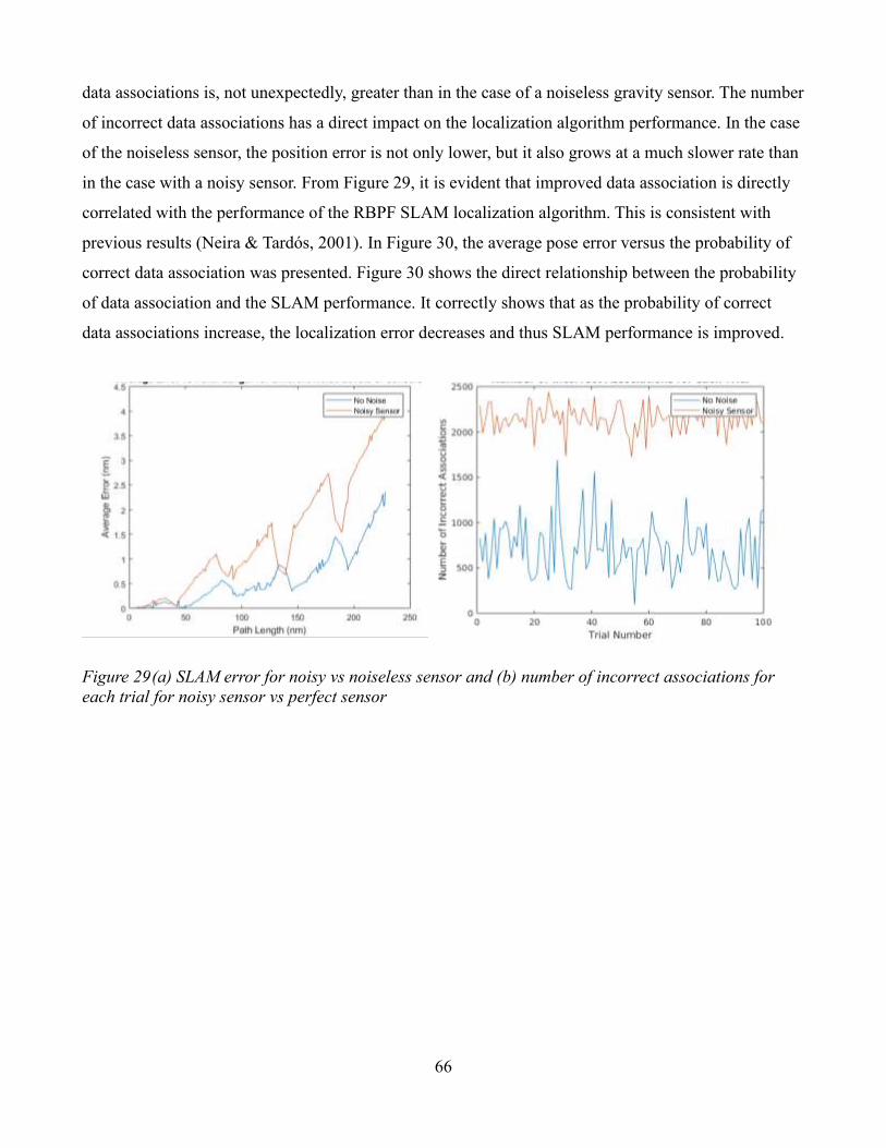
66

data associations is, not unexpectedly, greater than in the case of a noiseless gravity sensor. The number

of incorrect data associations has a direct impact on the localization algorithm performance. In the case

of the noiseless sensor, the position error is not only lower, but it also grows at a much slower rate than

in the case with a noisy sensor. From Figure 29, it is evident that improved data association is directly

correlated with the performance of the RBPF SLAM localization algorithm. This is consistent with

previous results (Neira & Tardós, 2001). In Figure 30, the average pose error versus the probability of

correct data association was presented. Figure 30 shows the direct relationship between the probability

of data association and the SLAM performance. It correctly shows that as the probability of correct

data associations increase, the localization error decreases and thus SLAM performance is improved.

Figure 29 (a) SLAM error for noisy vs noiseless sensor and (b) number of incorrect associations for

each trial for noisy sensor vs perfect sensor

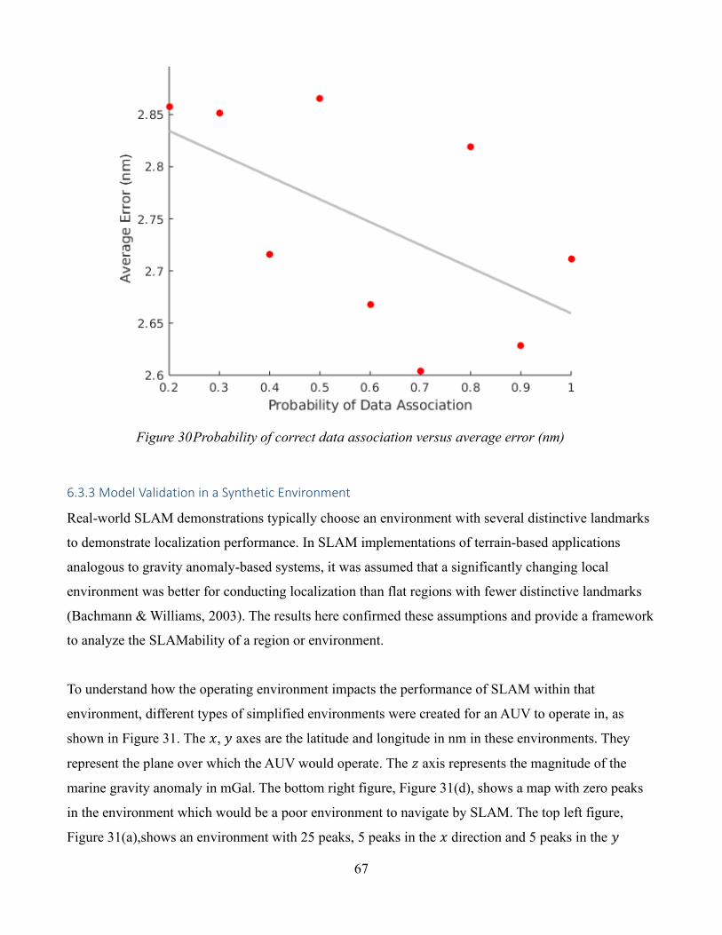
67

6.3.3 Model Validation in a Synthetic Environment

Real-world SLAM demonstrations typically choose an environment with several distinctive landmarks

to demonstrate localization performance. In SLAM implementations of terrain-based applications

analogous to gravity anomaly-based systems, it was assumed that a significantly changing local

environment was better for conducting localization than flat regions with fewer distinctive landmarks

(Bachmann & Williams, 2003). The results here confirmed these assumptions and provide a framework

to analyze the SLAMability of a region or environment.

To understand how the operating environment impacts the performance of SLAM within that

environment, different types of simplified environments were created for an AUV to operate in, as

shown in Figure 31. The 𝑥, 𝑦 axes are the latitude and longitude in nm in these environments. They

represent the plane over which the AUV would operate. The 𝑧 axis represents the magnitude of the

marine gravity anomaly in mGal. The bottom right figure, Figure 31(d), shows a map with zero peaks

in the environment which would be a poor environment to navigate by SLAM. The top left figure,

Figure 31(a),shows an environment with 25 peaks, 5 peaks in the 𝑥 direction and 5 peaks in the 𝑦

Figure 30 Probability of correct data association versus average error (nm)

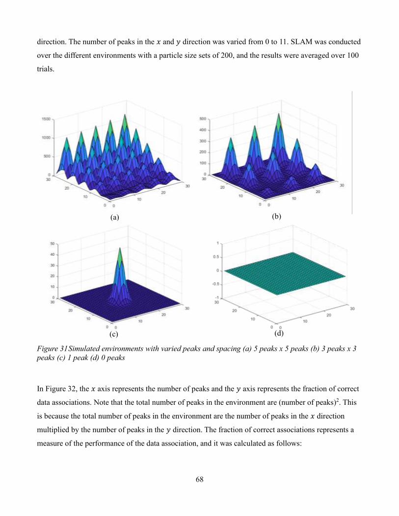
68

direction. The number of peaks in the 𝑥 and 𝑦 direction was varied from 0 to 11. SLAM was conducted

over the different environments with a particle size sets of 200, and the results were averaged over 100

trials.

In Figure 32, the 𝑥 axis represents the number of peaks and the 𝑦 axis represents the fraction of correct

data associations. Note that the total number of peaks in the environment are (number of peaks)2. This

is because the total number of peaks in the environment are the number of peaks in the 𝑥 direction

multiplied by the number of peaks in the 𝑦 direction. The fraction of correct associations represents a

measure of the performance of the data association, and it was calculated as follows:

Figure 31 Simulated environments with varied peaks and spacing (a) 5 peaks x 5 peaks (b) 3 peaks x 3

peaks (c) 1 peak (d) 0 peaks

(a) (b)

(c) (d)

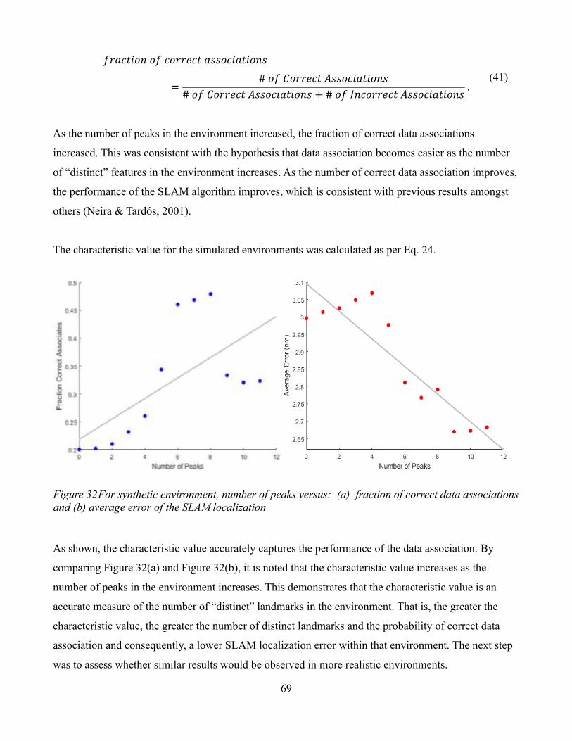
69

𝑓𝑟𝑎𝑐𝑡𝑖𝑜𝑛 𝑜𝑓 𝑐𝑜𝑟𝑟𝑒𝑐𝑡 𝑎𝑠𝑠𝑜𝑐𝑖𝑎𝑡𝑖𝑜𝑛𝑠

=# 𝑜𝑓 𝐶𝑜𝑟𝑟𝑒𝑐𝑡 𝐴𝑠𝑠𝑜𝑐𝑖𝑎𝑡𝑖𝑜𝑛𝑠

# 𝑜𝑓 𝐶𝑜𝑟𝑟𝑒𝑐𝑡 𝐴𝑠𝑠𝑜𝑐𝑖𝑎𝑡𝑖𝑜𝑛𝑠 + # 𝑜𝑓 𝐼𝑛𝑐𝑜𝑟𝑟𝑒𝑐𝑡 𝐴𝑠𝑠𝑜𝑐𝑖𝑎𝑡𝑖𝑜𝑛𝑠 .

(41)

As the number of peaks in the environment increased, the fraction of correct data associations

increased. This was consistent with the hypothesis that data association becomes easier as the number

of “distinct” features in the environment increases. As the number of correct data association improves,

the performance of the SLAM algorithm improves, which is consistent with previous results amongst

others (Neira & Tardós, 2001).

The characteristic value for the simulated environments was calculated as per Eq. 24.

As shown, the characteristic value accurately captures the performance of the data association. By

comparing Figure 32(a) and Figure 32(b), it is noted that the characteristic value increases as the

number of peaks in the environment increases. This demonstrates that the characteristic value is an

accurate measure of the number of “distinct” landmarks in the environment. That is, the greater the

characteristic value, the greater the number of distinct landmarks and the probability of correct data

association and consequently, a lower SLAM localization error within that environment. The next step

was to assess whether similar results would be observed in more realistic environments.

Figure 32 For synthetic environment, number of peaks versus: (a) fraction of correct data associations

and (b) average error of the SLAM localization

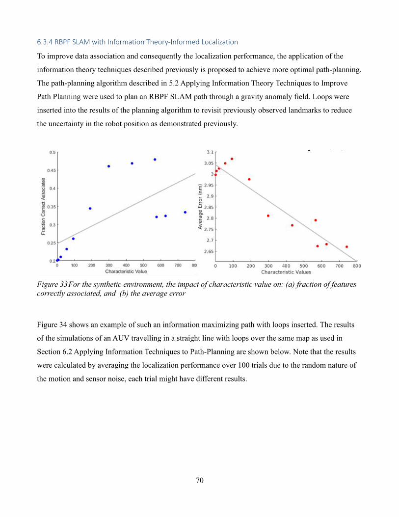
70

6.3.4 RBPF SLAM with Information Theory-Informed Localization

To improve data association and consequently the localization performance, the application of the

information theory techniques described previously is proposed to achieve more optimal path-planning.

The path-planning algorithm described in 5.2 Applying Information Theory Techniques to Improve

Path Planning were used to plan an RBPF SLAM path through a gravity anomaly field. Loops were

inserted into the results of the planning algorithm to revisit previously observed landmarks to reduce

the uncertainty in the robot position as demonstrated previously.

Figure 34 shows an example of such an information maximizing path with loops inserted. The results

of the simulations of an AUV travelling in a straight line with loops over the same map as used in

Section 6.2 Applying Information Techniques to Path-Planning are shown below. Note that the results

were calculated by averaging the localization performance over 100 trials due to the random nature of

the motion and sensor noise, each trial might have different results.

Figure 33 For the synthetic environment, the impact of characteristic value on: (a) fraction of features

correctly associated, and (b) the average error

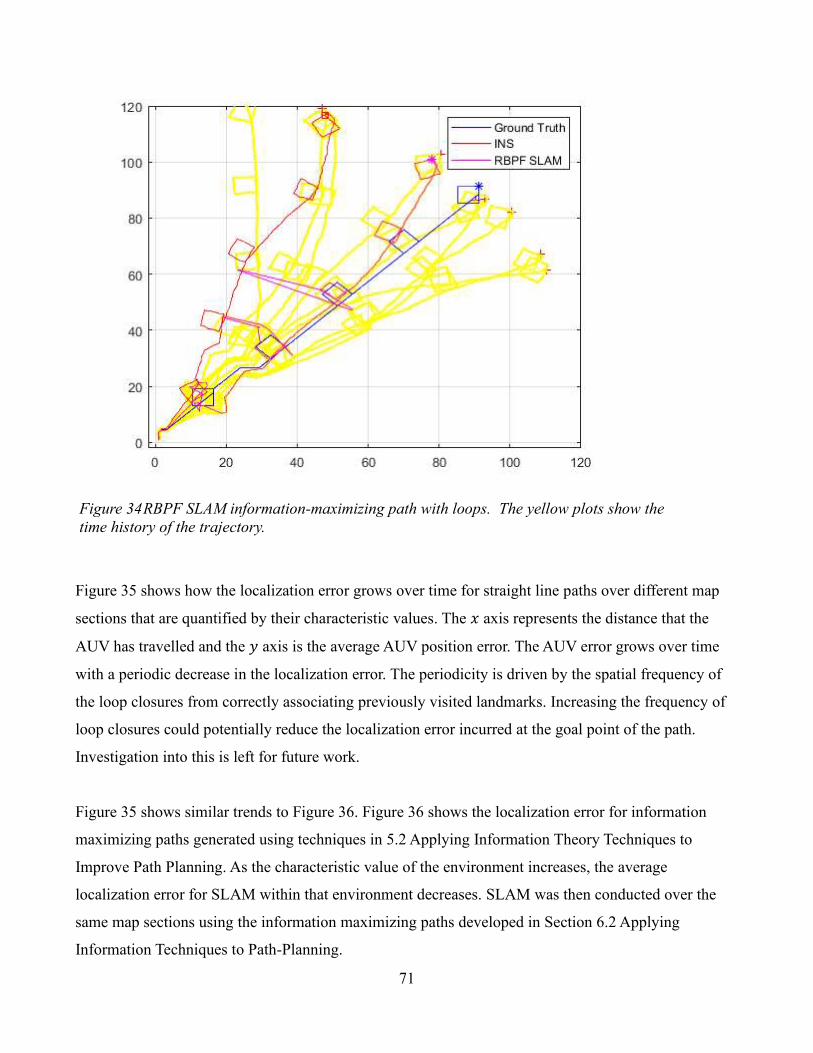
71

Figure 35 shows how the localization error grows over time for straight line paths over different map

sections that are quantified by their characteristic values. The 𝑥 axis represents the distance that the

AUV has travelled and the 𝑦 axis is the average AUV position error. The AUV error grows over time

with a periodic decrease in the localization error. The periodicity is driven by the spatial frequency of

the loop closures from correctly associating previously visited landmarks. Increasing the frequency of

loop closures could potentially reduce the localization error incurred at the goal point of the path.

Investigation into this is left for future work.

Figure 35 shows similar trends to Figure 36. Figure 36 shows the localization error for information

maximizing paths generated using techniques in 5.2 Applying Information Theory Techniques to

Improve Path Planning. As the characteristic value of the environment increases, the average

localization error for SLAM within that environment decreases. SLAM was then conducted over the

same map sections using the information maximizing paths developed in Section 6.2 Applying

Information Techniques to Path-Planning.

Figure 34 RBPF SLAM information-maximizing path with loops. The yellow plots show the

time history of the trajectory.

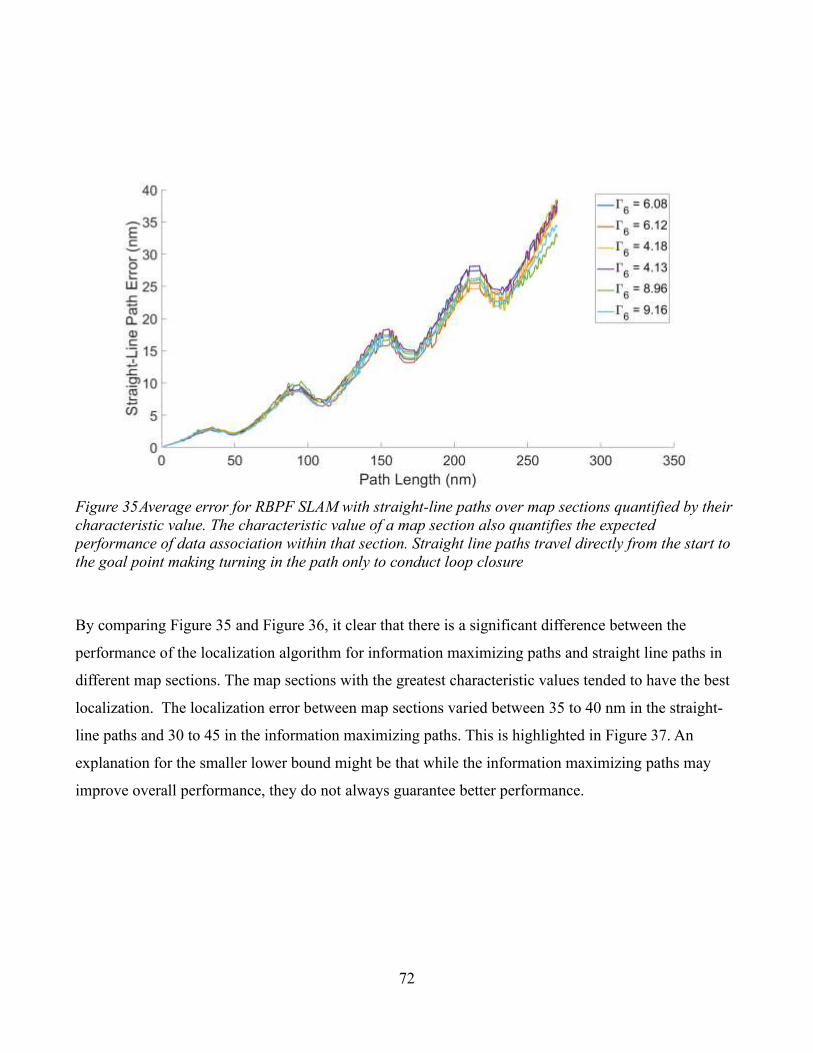
72

By comparing Figure 35 and Figure 36, it clear that there is a significant difference between the

performance of the localization algorithm for information maximizing paths and straight line paths in

different map sections. The map sections with the greatest characteristic values tended to have the best

localization. The localization error between map sections varied between 35 to 40 nm in the straight-

line paths and 30 to 45 in the information maximizing paths. This is highlighted in Figure 37. An

explanation for the smaller lower bound might be that while the information maximizing paths may

improve overall performance, they do not always guarantee better performance.

Figure 35 Average error for RBPF SLAM with straight-line paths over map sections quantified by their

characteristic value. The characteristic value of a map section also quantifies the expected

performance of data association within that section. Straight line paths travel directly from the start to

the goal point making turning in the path only to conduct loop closure

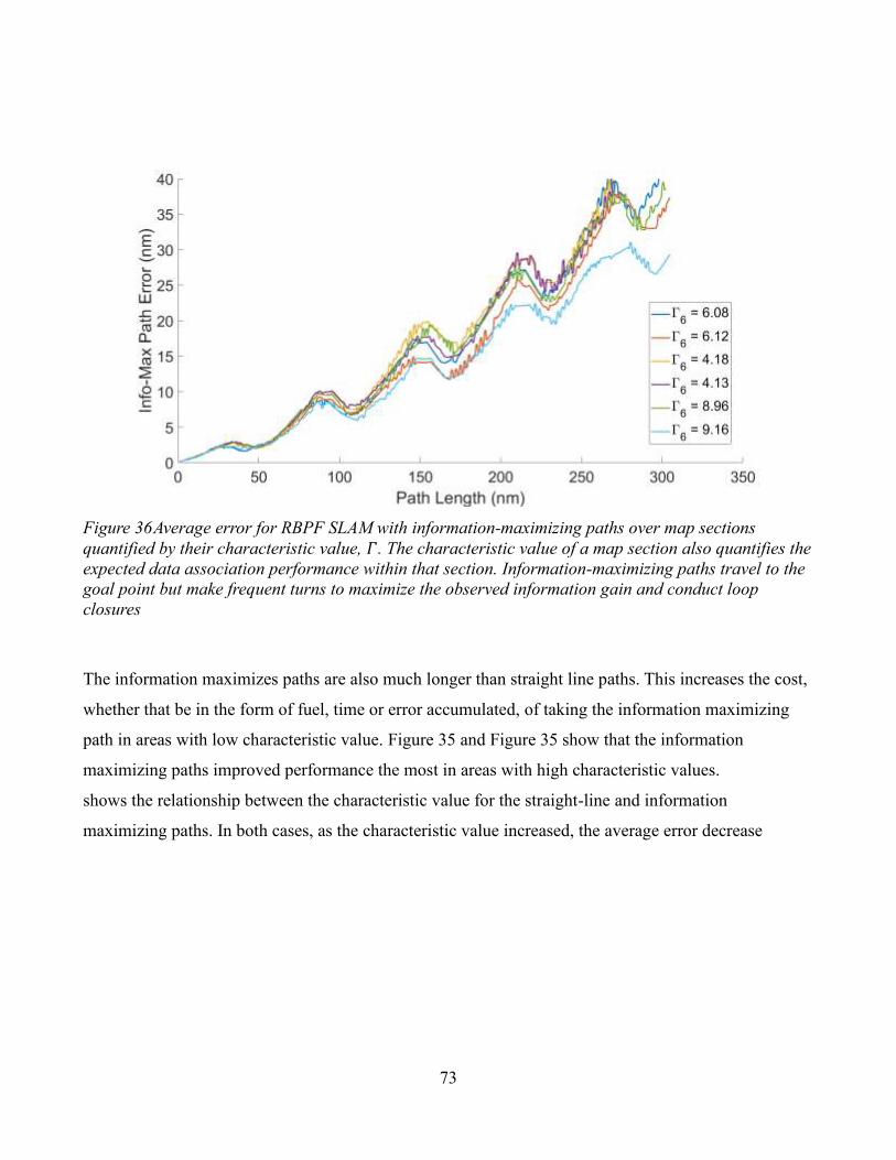
73

The information maximizes paths are also much longer than straight line paths. This increases the cost,

whether that be in the form of fuel, time or error accumulated, of taking the information maximizing

path in areas with low characteristic value. Figure 35 and Figure 35 show that the information

maximizing paths improved performance the most in areas with high characteristic values.

shows the relationship between the characteristic value for the straight-line and information

maximizing paths. In both cases, as the characteristic value increased, the average error decrease

Figure 36 Average error for RBPF SLAM with information-maximizing paths over map sections

quantified by their characteristic value, 𝛤. The characteristic value of a map section also quantifies the

expected data association performance within that section. Information-maximizing paths travel to the

goal point but make frequent turns to maximize the observed information gain and conduct loop

closures

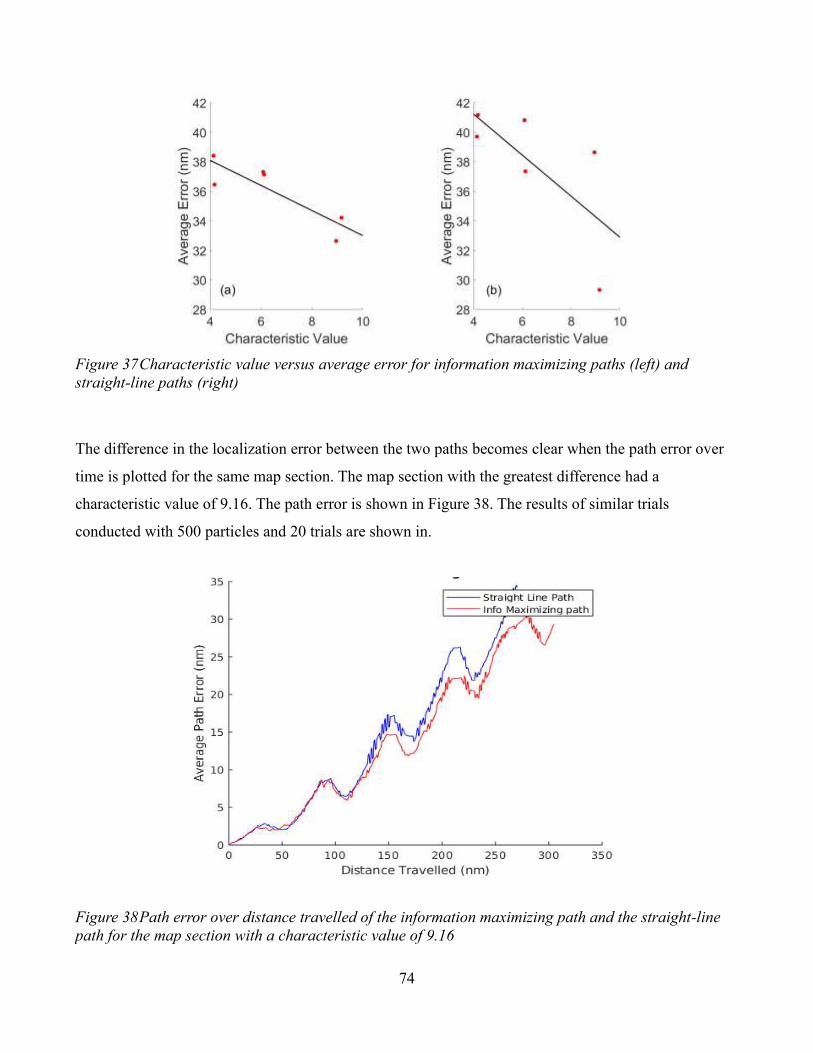
74

The difference in the localization error between the two paths becomes clear when the path error over

time is plotted for the same map section. The map section with the greatest difference had a

characteristic value of 9.16. The path error is shown in Figure 38. The results of similar trials

conducted with 500 particles and 20 trials are shown in.

Figure 37 Characteristic value versus average error for information maximizing paths (left) and

straight-line paths (right)

Figure 38 Path error over distance travelled of the information maximizing path and the straight-line

path for the map section with a characteristic value of 9.16

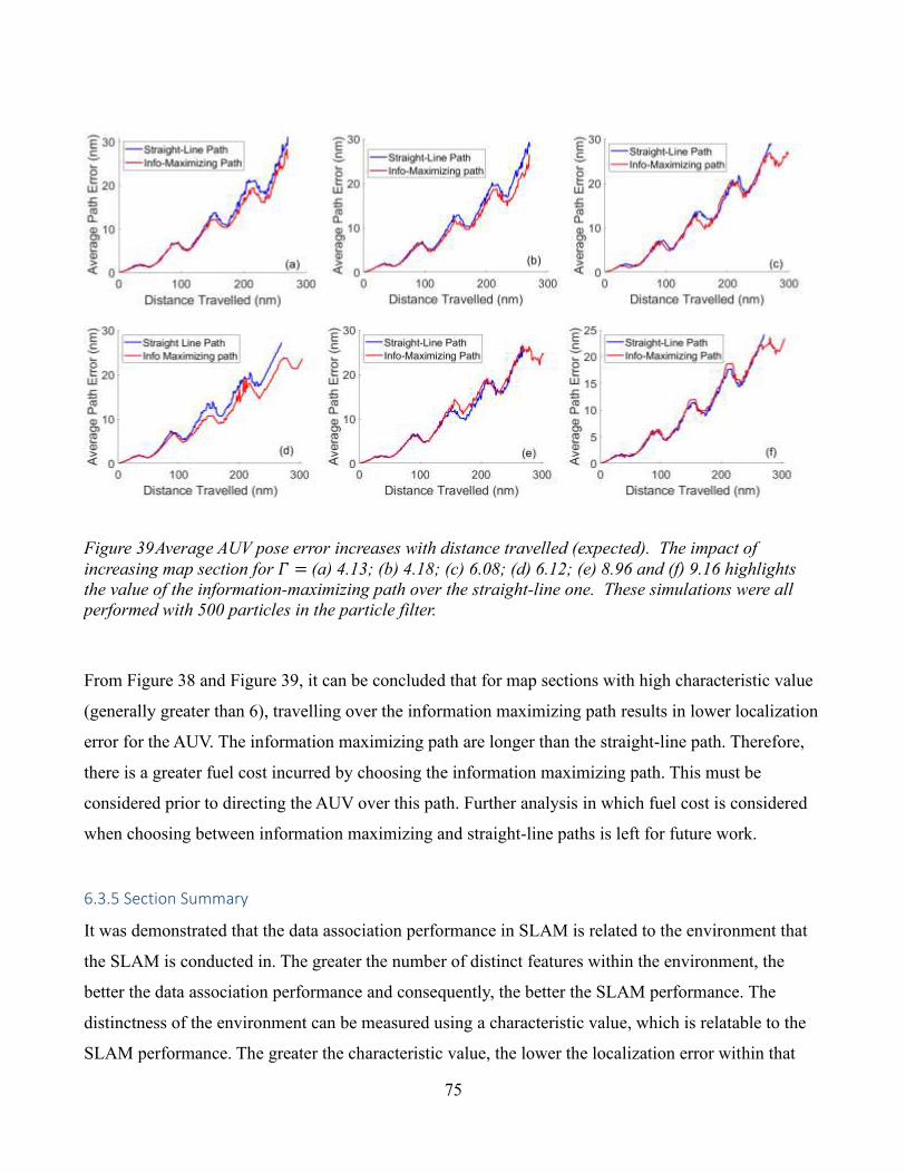
75

From Figure 38 and Figure 39, it can be concluded that for map sections with high characteristic value

(generally greater than 6), travelling over the information maximizing path results in lower localization

error for the AUV. The information maximizing path are longer than the straight-line path. Therefore,

there is a greater fuel cost incurred by choosing the information maximizing path. This must be

considered prior to directing the AUV over this path. Further analysis in which fuel cost is considered

when choosing between information maximizing and straight-line paths is left for future work.

6.3.5 Section Summary

It was demonstrated that the data association performance in SLAM is related to the environment that

the SLAM is conducted in. The greater the number of distinct features within the environment, the

better the data association performance and consequently, the better the SLAM performance. The

distinctness of the environment can be measured using a characteristic value, which is relatable to the

SLAM performance. The greater the characteristic value, the lower the localization error within that

Figure 39 Average AUV pose error increases with distance travelled (expected). The impact of

increasing map section for 𝛤 = (a) 4.13; (b) 4.18; (c) 6.08; (d) 6.12; (e) 8.96 and (f) 9.16 highlights

the value of the information-maximizing path over the straight-line one. These simulations were all

performed with 500 particles in the particle filter.

76

environment. It was also demonstrated that adopting the techniques proposed in Section 5.2 Applying

Information Theory Techniques to Improve Path Planning can have significant impact on the overall

SLAM performance. The results in Figure 35, Figure 36 and Figure 37 match the proposed results in

Figure 22, Figure 23 and Figure 24 of 6.2 Applying Information Techniques to Path-Planning.

77

Chapter 7 Summary of Results

7.1 Contributions

This thesis contributes to research in long-range underwater localization for GPS-denied environments.

There are three major areas of contribution. One, localization using gravity-based sensors is

demonstrated; initially with particle filter using an a priori map, and then with online RBPF SLAM

without the use of an a priori map. The implementation of RBPF SLAM without a sensor model or an

a priori map constitutes a novel contribution to the literature. Second, a characteristic value is shown to

be an effective method of evaluating the suitability of gravity anomaly maps for localization. Thus,

effectively allowing the characteristic value to be used as a “SLAMability” metric. Third, information

theory is applied to conduct path planning over a region using gravity-based maps. This results in an

AUV path that maximizes the distinctness of landmarks in the environment, thereby improving the data

association performance and consequently reducing the localization error. Taken together, the

contributions in this thesis could be used to realize real-world implementation of gravity-based

localization and navigation onboard AUVs.

7.2 Results

This thesis explores the feasibility of long-range underwater localization and navigation using gravity-

based sensors. This was first demonstrated by presenting a particle filter-based localization algorithm

that uses a priori gravity anomaly and vertical gravity gradient maps to perform localization. The

results of this localization were compared to the INS position, and the particle filter-based localization

algorithm demonstrated superior performance over a purely INS-based one. It was found that the

particle filter-based localization algorithm diverges depending on the characteristic value over which

the localization is conducted. Similar to the finding reported in (Wang, et al., Characteristics of Marine

Gravity Anomaly Reference Maps and Accuracy Analysis of Gravity Matching-Aided Naviation,

2017), this observation indicates that a relationship may exist between the characteristic value of a

region and the performance of the localization algorithm, but strong trends were not observed. This

might be due to the short distances over which the particle filter-based localization algorithm was

applied. As the primary goal is to conduct localization and navigation over long distances, it was

determined that conducting an analysis of a region prior to travelling through it would be beneficial. To

further investigate this relationship, simple models of INS-based localization and particle filter-based

localization were developed.

78

A simplified localization model was developed, which performs similarly to the particle filter-based

localization algorithm, by reducing the localization error when there were large changes in the local

gravity anomaly. The two models allowed simulations to be conducted over large map regions (on the

order of 100 nm) to investigate the relationship between the characteristic value of a region and the

localization error within that region. The results indicate that a weak relationship exists. Thus, a

different metric was considered for measuring the localization performance in a region prior to

travelling through it, which is based on the information theory metrics developed in (Baylog &

Wettergren, A search game for optimizing information collection in UUV mission planning, 2015).

Information theory techniques were used in conjunction with the A* path-planning algorithm to

determine information maximizing paths through various regions of gravity anomaly maps. Three

different types of paths from the start to the goal locations were planned. They were a straight-line path,

an information maximizing path, and a path based on the heuristic linear combination of the

information maximizing and distance minimizing approaches. The distance over which the analysis is

performed determines the optimal path type. Over short distances, the linear combination path showed

no advantage over the direct straight-line path to the goal location. Over long distances, the differences

between the three paths were more significant. The information maximizing path was the longest of the

three paths. A good tradeoff between the distance travelled and the information grained was achieved in

the linear combination path.

The resultant paths from the path-planning algorithm were simulated over map regions with different

characteristic values. There is a significant reduction in localization error for the information

maximizing path in regions with a high characteristic value. Thus, the characteristic value could be

used to predict the performance of a localization algorithm. Furthermore, the localization error was

significantly lower for long distances of travel. Conducting an analysis of a region prior to travelling

through it was found to be valuable, particularly over long distances, and so, the use of these techniques

to improve the performance of a SLAM-based system was considered.

As previously discussed, a SLAM-based localization system has several advantages over a matching-

based localization and navigation system. An RBPF SLAM localization system that uses a gravimeter

sensor was developed, and it was able to operate without an a priori map. Firstly, the impact of the

environment on the SLAM performance was considered. Artificial environments were constructed

79

consisting of varying numbers of peaks and spacings. As the number of peaks in an environment

increased, the performance of the data association algorithm improved. As the probability of correct

data association increased, the localization error of the SLAM algorithm decreased. These results are

consistent with previous results that have been reported in the literature, and they are in agreement with

our hypothesis. The characteristic value was calculated for the artificial environments created, and it

was found to increase as the number of peaks in the environment increased. These results suggest that

the characteristic value is a good measure of the “SLAMability” of the landmarks in the environment.

Consequently, as the characteristic value increased, the probability of correct data association within

that environment increased and the localization error of SLAM decreased.

These techniques were then applied to real world gravity anomaly maps. The results were consistent

with the hypothesis proposed using the simplified localization algorithm model. It was found that

regions with a high characteristic value tend to result in lower localization error. This was observed to

be true whether the AUV travelled over a straight-line path or an information maximizing path.

However, adopting the information maximizing paths resulted is better gravity-based RBPF SLAM

performance and reduced the localization error, particularly over long distances.

In this thesis, the characteristic value, which was first introduced in (Wang, et al., Characteristics of

Marine Gravity Anomaly Reference Maps and Accuracy Analysis of Gravity Matching-Aided

Naviation, 2017), has been shown to be an effective “SLAMability” metric for predicting the

performance of the SLAM algorithm.

80

Chapter 8 Future Work

There is still considerable work needed to advance this field. The problem of long-range underwater

localization and navigation has not been solved in this thesis, but promising progress was made. This

thesis compared the performance of gravity-based localization and navigation systems to that of an

onboard INS. Further studies could investigate how gravity-based systems perform compared to

systems using different external sensors such as a side scan sonar. The performance of the proposed

SLAM-based system could also be compared to existing ICCP or TERCOM-based algorithms.

Furthermore, there are outstanding questions with regards to the value of conducting frequent loop

closures. While the effectiveness of loop closures in reducing uncertainty and enabling long range

SLAM was demonstrated, the conditions under which this holds were not tested. Further research into

the frequency at which loop closures can be used is needed. If they can be used frequently without

accumulating excess error, then SLAM could be conducted at extremely long ranges.

In this implementation, the previous two most recently visited landmarks were revisited. However,

there may be more value in visiting the first landmark every time, and effectively conducting the full

localization plan multiple times. This still needs to be investigated, along with fuel analysis to

determine how much extra fuel is expended due to loop closure events and how this could be

minimized. Addressing these issues would allow future work to make use of effective route planning

techniques and explore further challenges in long-range SLAM-based localization.

In this thesis, the AUV path that maximizes the variability in gravity anomaly was determined to be the

information maximizing path. Future work could also integrate the vertical gravity gradient and thus,

the algorithm would optimize for a path that experiences the greatest variability in gravity anomaly and

vertical gravity gradient. Even greater information gain could be achieved along the resultant path,

which could further improve the localization performance.

Simulations of the error growth of the different paths also suggested that the navigation path that

conducts a tradeoff between minimizing the distance travelled and maximizing the information gain

would be the ideal paths to for long range navigation. These paths were not simulated with the SLAM

based system and are left for future work.

81

One of the major obstacles in this thesis was simulating SLAM at the long ranges that we are interested

in implementing it. This meant that the results of the simulations in this thesis were obtained using an

implementation of RBPF SLAM with lower number of particles than would typically chosen for the

problem. Further simulation with greater number of particles over a larger range of map sections would

produce clearer trends in the performance of SLAM over different map sections and different paths.

The feature-based SLAM approach selected in this thesis demonstrated that it was possible to treat

point measurements as landmarks. This approach does have limitations. Firstly, correctly data

associating each landmark becomes very important and the system is therefore not robust against

failure. Secondly, treating each measurement as a landmark lead to a large number of landmarks that

have to be maintained by each particle. This adds to the computational overhead of conducting SLAM.

A more realistic approach would be to implement grid-based SLAM. On a real-world gravity-based

system, the AUV would make measurements at the sampling frequency. This would be used to generate

an occupancy map of the environment which would use scan matching to associate previously visited

locations. A grid-based SLAM approach would also reduce the computational complexity of the

system.

Modern gravimeters can achieve accuracies on the order of µGals (1 µGals = 0.001 mGal) with the

error bias growing over time. Sensor noise from the gravimeter in this thesis was simulated using zero

mean Gaussian distributions with standard deviations of 5 mGal. A more accurate simulation would be

to simulate the growth in the sensor noise. This would violate the Markov assumption but could

potentially be used to improve SLAM performance.

As all the research in this thesis was conducted in simulation, the natural next step would be to

implement such a system onboard an AUV to demonstrate its practicality in the real world. While

considerable effort was expended to simulate real world conditions, there are likely obstacles to real

world implementation that are difficult to predict.

82

Chapter 9 Conclusion

The aim of this thesis was to demonstrate the feasibility of a gravity-based navigation system for long-

range underwater navigation. Such a system was demonstrated in simulation with the use of particle

filter-based localization and RBPF SLAM. Such a system allows an AUV to operate submerged for

extended periods of time without the use of an active sensor, thus widening the variety and type of

missions that an AUV can be employed for. Additionally, this thesis demonstrates how information

theory techniques can be exploited towards an a priori analysis of a region, which would provide a

“SLAMability” metric of the area that the AUV will operate in. This can inform the AUV on its

navigation success going through the region.

83

Bibliography

Anonsen, K. B. (2010). Advances in Terrain Aided Navigation for Underwater Vehicles.

Aulinas, J., Liado, X., Salvi, J., & Petillot, Y. R. (2010). Feature based slam using side-scan salient

objects. OCEANS 2010 MTS/IEEE SEATTLE.

Bachmann, A., & Williams, S. B. (2003). Terrain aided underwater navigation - A deeper insight into

generic monte carlo localization.

Bahr, A., Leonard, J. J., & Fallon, M. F. (2009). Cooperative Localization for Autonomous Underwater

Vehicles. The International Journal of Robotics Research.

Balanis, C. A. (2012). Advanced Engineering Electromagnetics. John Wiley & Sons, 2012.

Baylog, J. G., & Wettergren, T. A. (2015). A search game for optimizing information collection in UUV

mission planning. OCEANS 2015 - MTS/IEEE Washington.

Baylog, J. G., & Wettergren, T. A. (2017). A ROC-Based Approach for Developing Optimal Strategies

in UUV Search Planning. IEEE Journal of Oceanic Engineering, 843-855.

Biebauer, T. (2015). Gravimetric Methods - Absolute and Relative Gravity Meter: Instruments

Concepts and Implementation. In G. Schubert, Treatise on Geophysics (pp. 37-57). Elsevier.

Cadena, C., Carlone, L., Carrillo, H., Latif, Y., Scaramuzza, D., Neira, J., . . . Leonard, J. J. (2016).

Past, Present, and Future of Simultaneous Localization and Mapping: Toward the Robust-

Perception Age. IEEE Transations on Robotics, 1309-1332.

Che, X., Wells, I., Dickers, G., Kear, P., & Gong, X. (2010). Re-evaluation of RF electromagnetic

communication in underwater sensor networks. IEEE Communications Magazine, 143-151.

Corke, P., Detweiler, C., Dunbabin, M., Hamilton, M., Rus, D., & Vasilescu, L. (2007). Experiments

with Underwater Robot Localization and Tracking. Proceedings 2007 IEEE International

Conference on Robotics and Automation.

Debs, J. E., Hardman, K. S., Altin, P. A., McDonald, G., Close, J. D., & Robins, N. P. (2013). From

Apples to Atoms: Measuing gravity with ultra cold atomic test masses.

DiFFrancesco, D., Meyer, T., Christensen, A., & FitzGerald, D. (2009). Gravity gradiometry - today

and tomorrow. SAGA Biennial Technical Meeting and Exhibition, 80-83.

Douce, A., Godsill, S., & Andrieu, C. (2000). On sequential Monte Carlo sampling methods for

Bayesian filtering. Statistics and Computing, 197-208.

Dudek, G., Jenkin, M., Milios, E., & Wilkes, D. (1991). Robotic exploration as graph construction.

IEEE Transactions on Robotics and Automation, 859-865.

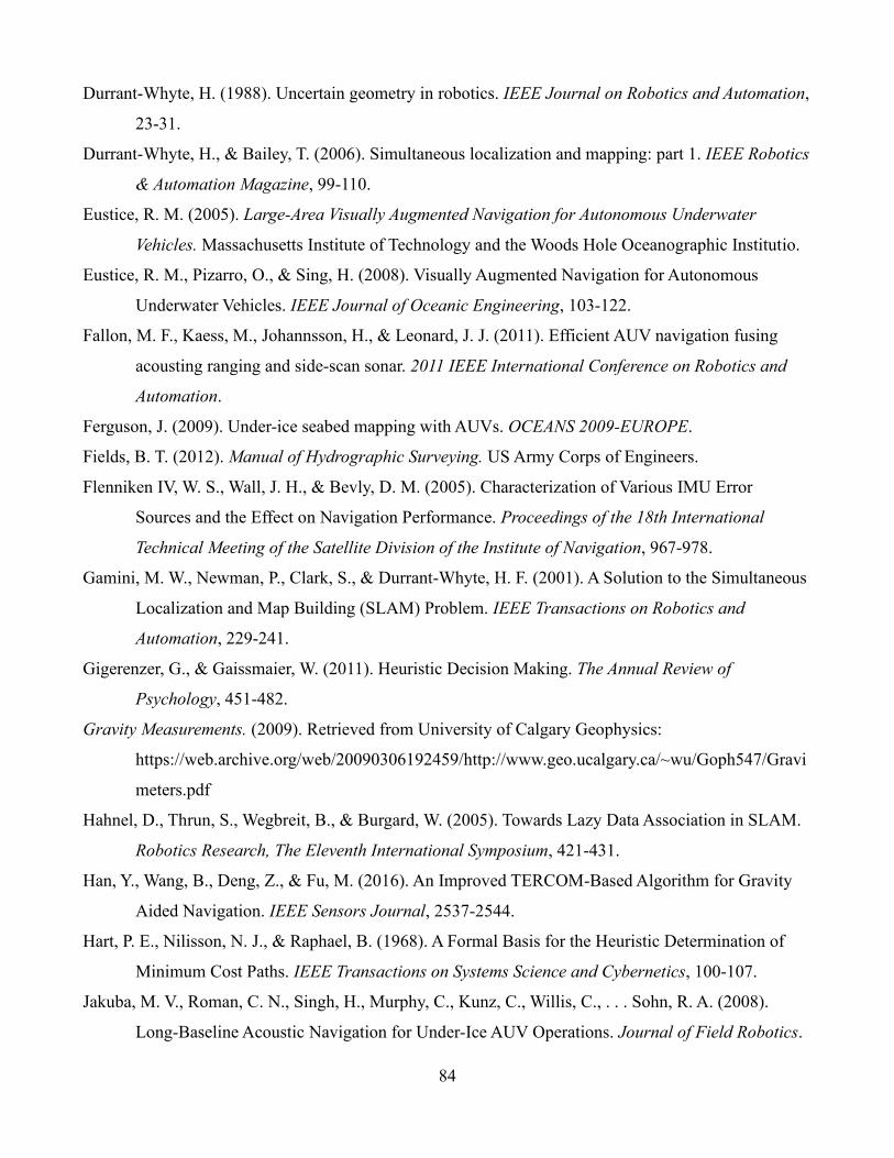
84

Durrant-Whyte, H. (1988). Uncertain geometry in robotics. IEEE Journal on Robotics and Automation,

23-31.

Durrant-Whyte, H., & Bailey, T. (2006). Simultaneous localization and mapping: part 1. IEEE Robotics

& Automation Magazine, 99-110.

Eustice, R. M. (2005). Large-Area Visually Augmented Navigation for Autonomous Underwater

Vehicles. Massachusetts Institute of Technology and the Woods Hole Oceanographic Institutio.

Eustice, R. M., Pizarro, O., & Sing, H. (2008). Visually Augmented Navigation for Autonomous

Underwater Vehicles. IEEE Journal of Oceanic Engineering, 103-122.

Fallon, M. F., Kaess, M., Johannsson, H., & Leonard, J. J. (2011). Efficient AUV navigation fusing

acousting ranging and side-scan sonar. 2011 IEEE International Conference on Robotics and

Automation.

Ferguson, J. (2009). Under-ice seabed mapping with AUVs. OCEANS 2009-EUROPE.

Fields, B. T. (2012). Manual of Hydrographic Surveying. US Army Corps of Engineers.

Flenniken IV, W. S., Wall, J. H., & Bevly, D. M. (2005). Characterization of Various IMU Error

Sources and the Effect on Navigation Performance. Proceedings of the 18th International

Technical Meeting of the Satellite Division of the Institute of Navigation, 967-978.

Gamini, M. W., Newman, P., Clark, S., & Durrant-Whyte, H. F. (2001). A Solution to the Simultaneous

Localization and Map Building (SLAM) Problem. IEEE Transactions on Robotics and

Automation, 229-241.

Gigerenzer, G., & Gaissmaier, W. (2011). Heuristic Decision Making. The Annual Review of

Psychology, 451-482.

Gravity Measurements. (2009). Retrieved from University of Calgary Geophysics:

https://web.archive.org/web/20090306192459/http://www.geo.ucalgary.ca/~wu/Goph547/Gravi

meters.pdf

Hahnel, D., Thrun, S., Wegbreit, B., & Burgard, W. (2005). Towards Lazy Data Association in SLAM.

Robotics Research, The Eleventh International Symposium, 421-431.

Han, Y., Wang, B., Deng, Z., & Fu, M. (2016). An Improved TERCOM-Based Algorithm for Gravity

Aided Navigation. IEEE Sensors Journal, 2537-2544.

Hart, P. E., Nilisson, N. J., & Raphael, B. (1968). A Formal Basis for the Heuristic Determination of

Minimum Cost Paths. IEEE Transactions on Systems Science and Cybernetics, 100-107.

Jakuba, M. V., Roman, C. N., Singh, H., Murphy, C., Kunz, C., Willis, C., . . . Sohn, R. A. (2008).

Long-Baseline Acoustic Navigation for Under-Ice AUV Operations. Journal of Field Robotics.

85

Jircitano, A., White, J., & Dosch, D. (1990). Gravity Based Navigation of AUVs. Symposium on

Autonomous Underwater Vehicle Technology.

Karlsson, R., & Gustafsson, F. (2003). Particle filter for underwater terrain navigation.

Kato, N., & Shigetomi, T. (2009). Underwater Navigation for Long-Range Autonomous Underwater

Vehicles Using Geomagnetic and Bathymetric Information . Advanced Robotics, 787-803.

Kuipers, B., & Byun, Y.-T. (1991). A robot exploration and mapping strategy based on a semantic

hierarchy of spatial representations. Robotics and Autonomous Systems, 47-63.

Melo, J., & Matos, A. (2013). On the use of Particle Fitlers for Terrain Based Navigation of sensor-

limited AUVs. IEEE Oceans.

Melo, J., & Matos, A. (2017). Survey on advances on terrain based navigation for Autonomous

Underwater Vehicles. Ocean Engineering, 250-264.

Middlemiss, R. P., Bramsiepe, S. G., Douglas, R., Hough, J., Paul, D. J., Rowan, S., & Hammond, G.

D. (2017). Field Tests of a Portable MEMS Gravimeter. Sensors.

Middlemiss, R., Samarelli, A., Paul, D. J., Hough, J., Rowan, S., & Hammond, G. (2016).

Measurement of the Earth tides with a MEMS gravimeter. Nature, 614-617.

Miller, P. A., Farrell, J. A., Zhao, Y., & Djapic, V. (2010). Autonomous Underwater Vehicle Navigation.

IEEE Journal of Oceanic Engineering, 663-677.

Montemerlo, M., Thrun, S., Koller, D., & Wegbreit, B. (2002). FastSLAM: A Factored Solution to the

Simultaneous Localization and Mapping Problem. Proceedings of the AAAI National

Conference on Artifical Intelligence.

Moryl, J., Rice, H., & Shinners, S. (1996). The unversal gravity module for enchanced submarine

navigation. IEEE 1998 Position Location and Navigation Symmposium.

Neira, J., & Tardós, J. D. (2001). Data Association in Stochastic Mapping Using the Joint Compatibility

Test. IEEE Transactions on Robotics and Automation, 890-897.

Newman, P., & Leonard, J. (2003). Pure range-only sub-sea SLAM. 2003 IEEE International

Conference on Robotics and Automation.

Nieto, J., Bailey, T., & Nebot, E. (2007). Recursive scan-matching SLAM. Robotics and Autonomous

Systems, 39-49.

Nygren, I. (2005). Terrain Navigation for Underwater Vehicles. Stockholm: KTH Electrical

Engineering.

O'Rourke, R. (2019). Navy Large Unmanned Surface and Undersea Vehicles: Background and Issues

for Congress. Congressional Research Service.

86

Pasnani, P., & Seto, M. (2018). Terrain-Based Localization and Mapping for Autonomous Underwater

Vehicles using Particle Filters with Marine Gravvity Anomalies. IFAC-PapersOnLine, 354-359.

Paull, L., Saeedi, S., Seto, M., & Li, H. (2014). AUV Navigation and Localization: A Review. IEEE

Journal of Oceanic Engineering, 131-149.

Quintas, J., Teixeira, F. C., & Pascoal, A. (2018). An Integrated System for Geophysical Navigation of

Autonomous Underwater Vehicles. IFAC Papers Online, 293-298.

Ridao, P., Carreras, M., Ribas, D., & Garcia, R. (2010). Visual inspection of hydroelectric dams using

an autonomous underwater vehicle. Journal of Field Robotics.

Rodriguez-Losada, D., Matia, F., Pedraza, L., Jimenez, A., & Galan, R. (2007). Consistency of SLAM-

EKF Algorithms for Indoor Environments. Journal of Intelligent and Robotic Systems, 375-397.

Salavasidis, G., Munafo, A., Harris, C. A., McPhail, S. D., Rogers, E., & Phillips, A. B. (2018).

Towards Arctic AUV Navigation. IFAC PapersOnLine, 287-292.

Sandwell, D. T., Muller, R. D., Smith, W. H., & Francis, R. (2014). New global marine gravity model

from CryoSat-2 and Jason-1 reveals buried tectonic structure. Science, 65-67.

Sariel, S., Balch, T., & Erdogan, N. (2008). Naval Mine Countermeasure Missions. IEEE Robotics &

Automation Magazine, 45-52.

Saxena, A., Sun, M., & Ng, A. Y. (2009). Make3D: Learning 3D Scene Structure from a Single Still

Image. IEEE Transactions on Pattern Analysis and Machine Intelligence, 824-840.

Schubert, G. (2015). Treatise on Geophysics. Elsevier.

Seto, M. L. (2013). Marine Robot Autonomy. New York: Springer.

Shinohara, M., Yamada, T., Ishihara, T., Araya, A., Kanazawa, T., Fujimoto, H., . . . Iizasa, K. (2015).

Development on an underwater gravity measurement system using autonomous underwater

vehicle for exploration of seafloor deposits. OCEANS 2015 - Genova.

Stachniss, C. (2013). Robot Mapping Course. Retrieved from University of Freiburg:

http://ais.informatik.uni-freiburg.de/teaching/ws13/mapping/

Teixeira, F. C., Pascoal, A., & Maurya, P. (2012). A Novel Particle Filter Formulation with Application

to Terrain-Aided Navigation. IFAC Proceedings Volumes, 132-139.

Thrun, S., Burgard, W., & Fox, D. (2005). Probabilistic Robotics. London: The MIT Press.

Tkhorenko, M. Y., Pavlov, B., Karshakov, E., & Volkovitsky, A. (2018). On integration of a strapdown

inertial navigation system with modern magnetic sensors. 2018 25th Saint Petersburg

International Conference on Integrated Navigation Systems (ICINS).

Vallivaara, I., Haverinen, J., Kemppainen, A., & Roning, J. (2011). Magnetic field-based SLAM

87

method for solving the localization problem in mobile robot floor-cleaning task. 2011 15th

International Conference on Advanced Robotics (ICAR).

Wang, H., Wu, L., Chai, H., Bao, L., & Wang, Y. (2017). Location Accuracy of INS/Gravity-Integrated

Navigation System on the Basis of Ocean Experiment and Simulation. Sensors.

Wang, H., Wu, L., Chai, H., Xiao, Y., Hsu, H., & Wang, Y. (2017). Characteristics of Marine Gravity

Anomaly Reference Maps and Accuracy Analysis of Gravity Matching-Aided Naviation.

Sensors.

Wang, Z., & Bian, S. (2008). A local geopotential model for implementation of underwater passive

navigation. Progress in Natural Science, 1139-1145.

Xiong, L., Ma, J., & Tian, J.-w. (2011). Gravity gradient aided position apprach based on EKF and NN.

Proceedings of 2011 Cross Strait Quad-Regional Radio Science and Wireless Technology

Conference.

Yu, J., Zhang, A., Li, Z., & Yan, K. (2004). The development and the challenges of underwater vehicles

for polar expedition. Proceedings of the 2004 International Symposium on Underwater

Technology.

Zeyu, W., & Srinivasan, R. S. (2017). A review of artificial intelligence based building energy use

prediction: Contrasting the capabilities of single and ensemble prediction models. Renewable

and Sustainable Energy Reviews, 796-808.