Long-Memory Dynamic Tobit Models

A.E. Brockwell∗ and N.H. Chan†

April 20, 2004

Abstract

We introduce a long-memory dynamic Tobit model, defining it as a censored versionof a fractionally-integrated Gaussian ARMA model, which may include seasonal com-ponents and/or additional regression variables. Parameter estimation for such a modelusing standard techniques is typically infeasible, since the model is not Markovian,cannot be expressed in a finite-dimensional state-space form, and includes censoredobservations. Furthermore, the long-memory property renders a standard Gibbs sam-pling scheme impractical. Therefore we introduce a new Markov chain Monte Carlosampling scheme, which is orders of magnitude more efficient than the standard Gibbssampler. The method is inherently capable of handling missing observations. In casestudies, the model is fit to two time series: one consisting of volumes of requests to ahard disk over time, and the other consisting of hourly rainfall measurements in Edin-burgh over a two-year period. The resulting posterior distributions for the fractionaldifferencing parameter demonstrate, for these two time series, the importance of thelong-memory structure in the models.

Keywords: Bayesian, censored, dynamic Tobit models, long-memory, Markov chain MonteCarlo, missing values, rainfall, time series, traffic volume.

1 Introduction

Models for censored Gaussian variables were formally introduced by Tobin (1958), whodemonstrated how they could be used to model househould expenditures on durable goods.In tribute to the author, these models were subsequently named “Tobit models”, and theirtime series counterparts are now typically referred to as “dynamic Tobit models”. Both

∗Dept. of Statistics, Carnegie Mellon University, Pittsburgh, PA, U.S.A.†Dept. of Statistics, Chinese University of Hong Kong, Shatin, N.T., Hong Kong

1

frequentist (Maddala, 1983) and Bayesian (Chib, 1992) methods have been developed foranalysis of (non-dynamic) Tobit models. Dynamic Tobit models, on the other hand, havesignificantly more complicated likelihood functions, and, until recently, have received some-what less attention. In earlier work, Zeger and Brookmeyer (1986) discuss (without explicitlylabeling them as such) an autoregressive form of dynamic Tobit model, and their applicationin modeling air-pollution data. In more recent work, Wei (1999) has given a useful Gibbssampling algorithm for their analysis, while Lee (1999) discusses simulation-based methodsfor parameter estimation.

Since their introduction, dynamic Tobit models have been applied in a variety of settings. Inaddition to the air-pollution study in Zeger and Brookmeyer (1986), an analysis of Japanesecar exports to the U.S. given in Wei (1999), and a number of other applications which arereferred to in Wei (1999) and Lee (1999), Brockwell et al. (2003) have recently used dynamicTobit models to analyze time series of disk-traffic and ethernet traffic volume. Such timeseries are of particular interest to computer scientists, since good models could in theory beused to develop tools which automate various system administration tasks. These time seriesare known to exhibit several properties. They are typically “bursty”, meaning that activitytends to occur in localized regions in time, and are also highly non-Gaussian, with a strongseasonal component. (see, e.g. Hinich and Molyneux, 2003; Resnick, 2004, for more detailsand discussion). All of these properties can be (to some extent) captured with dynamicTobit models. Another nice application appears in Glasbey and Nevison (1997), where themodels are used to describe hourly rainfall data recorded in Edinburgh.

Recently, it has been argued that a number of time series in the aforementioned fields exhibitthe “long-memory property”, that is, their autocovariance functions decay slower than ex-ponentially (for more details on long-memory processes, see, e.g. Granger and Joyeux, 1980;Hosking, 1981; Beran, 1994). In particular, Willinger et al. (1997) argue that time seriesmeasuring network traffic are long-memory processes, and Beran (1994) also gives examplesof ethernet traffic volume data which exhibits long memory properties. While the dynamicTobit model proposed by Brockwell et al. (2003) can capture the burstiness, non-Gaussianity,and seasonal patterns in such time series, it cannot capture long-memory properties. Inter-estingly, the rainfall data studied by Glasbey and Nevison (1997) also appears to exhibitlong-memory properties. (As the authors note, about the autocorrelation function of thetime series, “the rate of decay is not exponential, ..., both short term effects, ..., and per-sistent correlations, ..., are apparent.” They deal with this by constructing a model for thelatent Gaussian process which can be regarded as a combination of linear combination offour processes, each with a different rate of decay in the autocovariance function.) Thesetwo examples, in particular, suggest the potential usefulness of long-memory versions of dy-namic Tobit models, and we believe that such models could be useful in a wider range ofsettings. However, to our knowledge, explicit methods for analysis of such models have notbeen developed.

In this paper, we define a long-memory dynamic Tobit (LMDT) model as a censored ver-sion of a Gaussian fractionally integrated autoregressive moving average (ARFIMA) model.The model generalizes previously-studied models in two senses. Not only does it provide

2

a means of capturing long-memory properties, but in contrast with previous definitions ofdynamic Tobit models, it also allows for a richer range of possible autocovariance structuresby introducing moving average coefficients. Unfortunately, for this class of models, existingmethods for inference become infeasible. Direct maximum likelihood estimation cannot becarried out since the likelihood in this case is a high-dimensional integral over possible valuesof the censored observations. A natural alternative approach is to use a Markov chain MonteCarlo sampling scheme (see, e.g. Gilks et al., 1996, for many details on MCMC methods).For instance, following the approach adopted in earlier work of Carlin et al. (1992), onecould use the Gibbs sampler to update values of parameters as well as values of the underly-ing ARFIMA process, or alternatively, one could use the Gibbs sampling scheme developedspecifically for dynamic Tobit models by Wei (1999). In fact, neither of these two approachesis directly applicable to the class of models considered in this paper. The ARFIMA modelcannot be cast into the state-space form required in Carlin et al. (1992), and the approachof Wei (1999) is not directly generalizable to the case where the latent process has eithermoving average or long-memory structure. (Note also that the particle filtering approachdiscussed in Andrieu and Doucet (2002) is not practical to use, since ARFIMA models arenon-Markovian, and cannot be expressed in fixed-dimensional state-space form.) One couldof course fall back on the simplest version of the Gibbs sampler, regarding censored valuesof the ARFIMA process as additional parameters to be updated. However, this would re-quire enormous computational effort. Since the hidden state process is long-memory, thefull conditional distributions of the states would depend on all other hidden states, not justone or two. Therefore we introduce a new sampling scheme for updating the hidden states.Instead of using the Gibbs sampler (as described, for instance, by Carlin et al., 1992), weuse an MCMC scheme in which proposals for hidden states come from one-step predictivedistributions instead of full-conditional distributions. This enables us to avoid the necessityof casting the model in state-space form, and furthermore provides an efficient way to re-usecomputations during a scan of updates to the hidden values of the ARFIMA process. As anadded convenience, the scheme is particularly well-suited to handle missing values.

We demonstrate the application of the technique in two case studies. In the first, we re-visit the disk-trace time series analyzed in Brockwell et al. (2003), fitting the long-memoryversion of the original model, and in the second, we fit the model to a portion of the Edin-burgh rainfall data analyzed in Glasbey and Nevison (1997). In both cases, the fractionaldifferencing parameter is estimated along with other model parameters, and we find thatits posterior distribution strongly indicates the superiority of the LMDT model over thestandard dynamic Tobit model.

2 The Model

We define the long-memory dynamic Tobit model by

Yt = g(Xt + uTt β), (1)

3

where the function g(x) = max(x, c) censors the real-valued observations {Yt} at the thresh-old c, {ut ∈ Rr} is some exogenous vector-valued process, and β = (β1, . . . , βr)

T is a vectorof coefficients. {Xt} is assumed to be a latent stationary zero-mean ARFIMA(p, d, q) processsatisfying

φ(B)(1−B)dXt = ϑ(B)Zt, (2)

where B denotes the backshift operator, φ(B) = 1−∑p

i=1 φiBi, ϑ(B) = 1 +

∑qi=1 ϑiB

i, the“fractional differencing parameter” d is a constant in the range (−0.5, 0.5), {Zt} is an iidGaussian noise sequence with mean zero and variance σ2, and the roots of the polynomialsφ(·) and ϑ(·) lie strictly outside the unit circle. The fractional differencing operator (1−B)d

is interpreted in the usual manner (see, e.g. Beran, 1994) as

(1−B)d =∞∑

k=0

Γ(d+ 1)

Γ(k + 1)Γ(d− k + 1)(−1)kBk.

In the case studies considered in this paper, we use the term uTt β to introduce non-zero means

and periodic seasonal components, but in principle, it could also be used to accomodatetrends (linear, quadratic, spline, etc.), and/or any other covariates of interest.

3 Parameter Estimation and Forecasting

Our goal is, given observations Y = {yt1 , yt2 , . . . , ytM}, with 1 = t1 < t2 < . . . < tM = N ,to estimate the parameter vector θ = (β1, . . . , βr, φ1, . . . , φp, ϑ1, . . . , ϑq, σ, d), using an exactlikelihood-based method. (Typically, we would have ti = i, unless some observations aremissing.) We also aim to obtain predictive distributions p(YN+1, . . . , YN+h|Y ) for some non-negative integer-valued forecast horizon h. For convenience we define X = (X1, . . . , XN) andθ = (θ1, . . . , θn).

If X were observed, then the likelihood would be straightforward to obtain, using for in-stance methods proposed by Sowell (1992) (see also Doornik and Ooms, 2003, for a numberof additional useful computational details). However, in the model (1,2), X is unobserved,and hence the likelihood is much more difficult to compute, since every censored observationintroduces an extra integration operator into the expression for the likelihood. Furthermore,standard filtering techniques, for instance the particle filter, cannot be applied to the prob-lem, since the long-memory property precludes X from being cast into finite-dimensionalstate-space form in the usual manner (see, e.g. Brockwell and Davis, 1991, or other standardtexts).

Therefore we analyze the problem within a Bayesian framework, adopting a Markov chainMonte Carlo (MCMC) approach similar to that used in Carlin et al. (1992); Brockwell et al.(2003). The general approach is as follows.

4

Algorithm 3.1:

Step 0. Initialization. Set k = 0 and choose some initial states X(k) ={X(k)

1 , . . . , X(k)N }, θ(k) which are consistent with the observations in the

sense that Yt = g(X(k)t + uT

t β(k)) for t = 1, 2, . . . , N.

Step 1. Set θ(k+1) = θ(k), and X(k+1) = X(k). Replace k by k + 1.

Step 2. State updates. For t = 1, . . . , N , update X(k)t by a Metropolis-

Hastings update.

Step 3. Parameter updates. Update the components of θ(k) by Metropolis-Hastings updates.

Step 4. Forecasting. Generate a simulation X(k)N+1, . . . , X

(k)N+h of future val-

ues of the process, given {X(k)1 , . . . , X

(k)N } and θ(k). Then compute cor-

responding values Y(k)N+1, . . . , Y

(k)N+h.

Step 5. Go back to Step 1.

Step 3 is usually referred to as a “scan”, and is typically the most computationally intensivepart of the algorithm. The algorithm can be executed indefinitely, and in the long run, thevalues (X(k), θ(k)), k = 1, 2, . . . , at the end of each scan can be regarded as draws from theposterior distribution

π(θ,X) ∝ p(X, Y, θ) = p(Y |X, θ)p(X|θ)p(θ), (3)

where p(θ) is some prior distribution assigned to the unknown parameters. Furthermore, fore-

cast values Y(k)N+j can be regarded as draws from the predictive distribution p(YN+j|Y1, . . . , YN).

The joint likelihood p(X,Y, θ) is straightforward to compute. In the factorization (3),p(Y |X, θ) is simply an indicator function equal to one if and only if Y is consistent withX, i.e. if Yt = g(Xt + uT

t β) for all t, and p(X|θ) is the likelihood of the ARFIMA(p, d, q)process X, which can be computed by first finding the autocovariance function γX(h) forlags h = 0, 1, 2, . . . , N − 1, and then applying the Durbin-Levinson algorithm (see Durbin,1960) to obtain one-step predictors

X̂t+1 = E [Xt+1|Xt, . . . , X1] =t∑

j=1

αt,jXt+1−j (4)

and their mean squared errors

νt = E[(Xt+1 − X̂t+1)

2|Xt, . . . , X1

]. (5)

The log-conditional likelihood is then

log p(X|θ) = −N log(2π)/2 +N∑

t=1

log(νt−1)/2 +N∑

t=1

(Xt − X̂t)2/(2νt−1). (6)

5

Details on computation of the autocovariance function γX(·), and the Durbin-Levinson al-gorithm are given in Appendix A.

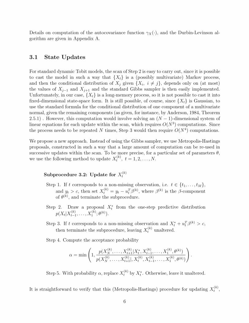
3.1 State Updates

For standard dynamic Tobit models, the scan of Step 2 is easy to carry out, since it is possibleto cast the model in such a way that {Xt} is a (possibly multivariate) Markov process,and then the conditional distribution of Xj given {Xi, i 6= j}, depends only on (at most)the values of Xj−1 and Xj+1 and the standard Gibbs sampler is then easily implemented.Unfortunately, in our case, {Xt} is a long-memory process, so it is not possible to cast it intofixed-dimensional state-space form. It is still possible, of course, since {Xt} is Gaussian, touse the standard formula for the conditional distribution of one component of a multivariatenormal, given the remaining components (as given, for instance, by Anderson, 1984, Theorem2.5.1) . However, this computation would involve solving an (N − 1)-dimensional system oflinear equations for each update within the scan, which requires O(N3) computations. Sincethe process needs to be repeated N times, Step 3 would then require O(N4) computations.

We propose a new approach. Instead of using the Gibbs sampler, we use Metropolis-Hastingsproposals, constructed in such a way that a large amount of computation can be re-used insuccessive updates within the scan. To be more precise, for a particular set of parameters θ,we use the following method to update X

(k)t , t = 1, 2, . . . , N.

Subprocedure 3.2: Update for X(k)t

Step 1. If t corresponds to a non-missing observation, i.e. t ∈ {t1, . . . , tM},and yt > c, then set X

(k)t = yt − uT

t β(k), where β(k) is the β-component

of θ(k), and terminate the subprocedure.

Step 2. Draw a proposal X∗t from the one-step predictive distribution

p(Xt|X(k)t−1, . . . , X

(k)1 ; θ(k)).

Step 3. If t corresponds to a non-missing observation and X∗t + uT

t β(k) > c,

then terminate the subprocedure, leaving X(k)t unaltered.

Step 4. Compute the acceptance probability

α = min

(1,

p(X(k)N , . . . , X

(k)t+1|X∗

t , X(k)t−1, . . . , X

(k)1 , θ(k))

p(X(k)N , . . . , X

(k)t+1|, X

(k)t , X

(k)t−1, . . . , X

(k)1 , θ(k))

).

Step 5. With probability α, replaceX(k)t byX∗

t . Otherwise, leave it unaltered.

It is straightforward to verify that this (Metropolis-Hastings) procedure for updating X(k)t ,

6

retains π(θ,X) as the invariant distribution of the Markov chain. Furthermore the log of theratio in the expression for α in Step 4 can be simplified to

log

[p(X

(k)N , . . . , X

(k)t+1|X∗

t , X(k)t−1, . . . , X

(k)1 , θ(k))

p(X(k)N , . . . , X

(k)t+1|X

(k)t , X

(k)t−1, . . . , X

(k)1 , θ(k))

]

=N∑

j=t+1

[(X∗j − X̂∗

j )2 − (Xj − X̂j)2]/(2νj−1), (7)

where X∗t is the proposal from Step 2, X∗

j = Xj for j 6= t, and

X̂∗j =

j−1∑i=1

αj−1,iX∗j−i, (8)

{αt,j} being the coefficients in (4). The Durbin-Levinson algorithm computes all the requiredone-step predictors and their mean-squared errors, in O(N2) computations, and if this pro-cedure were to be repeated N times, as required for a complete scan, the total computationaleffort for a scan would be O(N3).

While use of Subprocedure 3.2 within the scan provides a substantial improvement over theO(N4) approach mentioned above, it is possible to further improve efficiency when the coef-ficients {αt,j, t = 1, 2, . . . , N, j = 1, 2, . . . , t} can be stored. Suppose that Subprocedure 3.2

is supplied with X̂1, . . . , X̂N , as well as ν0, . . . , νN−1, and the coefficients {αt,j}. Then the

proposal X∗t can be drawn directly from a N(X̂t, νt−1) distribution. Furthermore, it follows

from equations (4) and (8) that

X̂∗j =

{X̂j, j ≤ t,

X̂j + αj−1,j−t(X∗t −Xt), j > t.

(9)

Thus, using equations (7) and (9), the acceptance probability in Step 4 can be computedin O(N) operations. Next note throughout the scan, the parameter vector θ is not altered.Thus the autocovariance function γX(·), the coefficients {αt,j}, and the one-step predictivemean-squared errors νt remain constant, and can be computed just once for the entire scan,at a cost of O(N2) computations using the Durbin-Levinson Algorithm. Also observe that itis possible to keep track of the current values of {X̂j, j = 1, . . . , N} as the scan progresses.

At the end of each state-update, {X̂j} remains the same if Xt was not updated, otherwise, it

is replaced by {X̂∗j }. Thus the entire scan requires the initial O(N2) computations, as well

as an additional N times O(N) computations, for a total of O(N2) operations.

3.2 Parameter Updates

Step 3 of Algorithm 3.1 requires parameter values θ(k)j , j = 1, 2, . . . , n to be updated by

Metropolis-Hastings steps. This is a straightforward procedure, and one way of carrying

7

it out is as follows. (Recall that θ(k) = (β(k)1 , . . . , β

(k)r , θ

(k)r+1, . . . , θ

(k)n ) consists of regression

parameters β1, . . . , βr as well as ARFIMA parameters.)

For j = r + 1, . . . , n (that is, for non-regression parameters), one can draw a proposal θ∗jfrom a density gj(θj, ·), compute the acceptance probability

α = min

(1,

p(X|θ∗)gj(θj; θ∗j )

p(X|θ(k))gj(θ∗j ; θj)

),

and, with probability α, replace θ(k) by θ∗j .

For j = 1, . . . , r, θ(k)j corresponds to the regression parameter β

(k)j , and the update needs

to be handled more carefully, since a proposed change to a component of β could result inchanges to many elements of the time series {Xt + utβ, t = 1, . . . , N}. Since p(Yt|Xt) isan indicator function, such a change typically causes the likelihood p(Y |X) =

∏t p(Yt|Xt)

to become zero, which in turn leads to rejection of the proposal. A much more effi-cient method is to draw a proposal β∗j from the density hj(β

(k)j , ·), then generate a cor-

responding state proposal X∗ = (X∗1 , . . . , X

∗N), X∗

t = X(k)t + ut(β

(k) − β∗), where β∗ =

(β(k)1 , . . . , β

(k)j−1, β

∗j , β

(k)j+1, . . . , β

(k)r )T . This proposal allows βj to change, while preserving the

values of {X(k)t + utβ}.) Then the acceptance probability is simply

α = min

(1,p(X∗|θ∗)hj(β

∗j , β

(k)j )

p(X|θ)hj(β(k)j , β∗j )

),

with θ∗ = (β∗, φ(k)1 , . . . , σ(k), d(k)).

4 Case Studies

4.1 Disk-Trace Data

Brockwell et al. (2003) proposed the use of Tobit models for Box-Cox-transformed trafficvolume time series. The particular models they fit can be regarded as special cases of theLMDT model (1,2), with p = 1, d = 0, and q = 0. Using the technique described in theprevious section, we fit the full LMDT model to the data, with parameters p = 1 and q = 0,but allowing d to vary.

We re-analyzed one of the time series studied in Brockwell et al. (2003), which was collectedfrom a hard disk of a Hewlett Packard workstation (named hplajw and described in Ruemmlerand Wilkes, 1993). During the time period from 12:00 AM, Sat., Apr. 18, 1992 to 11:00 PM,Fri., Jun. 19, 1992 (almost 63 days), the size in bytes of each job read from the hard disk wasrecorded, together with its arrival time, transferral time and the storage location (sector).

8

Job sizes in successive 30 minute intervals were then aggregated. Finally, before fitting themodel, in order to ensure that the marginal distributions are “close” to censored Gaussiandistributions (see Section 4.1 of Brockwell et al., 2003, for more details), we transformed thedata by a Box-Cox transformation with parameter 0.24. The resulting time series is shownin Figure 1.

500 1000 1500 2000 2500 3000

40

60

80

100

120

140

160

180

200

220

240

Time in Half−hour Units

Box

−Cox

(Vol

ume

in B

ytes

)

Figure 1: Box-Cox transformation, parameter λ = 0.24, of thetotal volume in bytes of read-requests to a hard disk in a HewlettPackard workstation, aggregated in half-hour blocks. Data wasrecorded from 12:00 AM, Apr. 18th, 1992 to 11:00 PM, Jun. 19th,1992.

In the LMDT model for this data, {Xt} was an ARFIMA(1,d,0) process, and the seasonalstructure was described by uT

t β = vt +βwIw(t), where {vt} is a seasonal component of period48 (one day) satisfying vt+48 = vt, Iw(t) is an indicator function equal to one when t lies ina weekend or holiday, and βw is a week-end effect. Thus we use β = (v1, . . . , v48, βw), andset ut to be the design matrix required to pick out the appropriate components of β.

Using the procedure described in Section 3, we generated 10,000 iterations of a Markov chainwhose limiting distribution is the posterior distribution of θ and X, given the observationsY . We chose uninformative priors for σ and β, and uniform priors for φ and d, on the ranges(−1, 1) and (−0.5, 0.5), respectively. We discarded the first 1,000 iterations as “burn-in”,and used the remaining 9,000 as samples from the posterior. Kernel-smoothed plots of theposterior density of the four parameters φ, d, σ and βw are shown in Figure 2, while Figure 3shows the posterior mean for each of the seasonal components v1, . . . , v48.

Posterior means of parameters obtained for both the long-memory Tobit model and themodel of Brockwell et al. (2003) are given in Table 1. The seasonal components, as well as

9

−0.4 −0.2 0.0 0.2 0.4

02

46

810

Posterior Density of Phi

N = 9000 Bandwidth = 0.005741

Den

sity

−0.4 −0.2 0.0 0.2 0.4

05

1015

Posterior Density of d

N = 9000 Bandwidth = 0.003561

Den

sity

0 20 40 60 80 100

0.00

0.10

0.20

0.30

Posterior Density of Sigma

N = 9000 Bandwidth = 0.1604

Den

sity

−100 −80 −60 −40 −20 0

0.00

0.02

0.04

0.06

0.08

0.10

Posterior Density of Weekend Effect

N = 9000 Bandwidth = 0.5565

Den

sity

Figure 2: Kernel-smoothed posterior densities obtained using theMCMC simulation approach, for the disk trace data.

XXXXXXXXXXXXParam.Model

BCL LMDT

φ 0.532(0.478,0.592) 0.049(-0.027,0.124)d 0.000(0.000,0.000) 0.305(0.257,0.354)σ 50.94(47.87,54.54) 47.19(45.18,49.24)βw -19.58(-44.53,-1.39) -56.15(-64.08,-48.51)

Table 1: Posterior Means (95% credible intervals) for model param-eters for the disk-trace data.

10

0 5 10 15 20

050

100

Daily Seasonal Pattern

Time in Hours

Leve

l

Figure 3: The posterior means of the daily seasonal pattern,v1, . . . , v48, for the disk-trace data.

parameters βw and σ, are quite close to those obtained in Brockwell et al. (2003). In theLMDT model, although the posterior mean of the autoregressive parameter φ is noticeablysmaller than that obtained for the BCL model, it is worth noting that the autocorrelationfor the two models (using the posterior mean as a fitted value) is almost identical at lag one.At higher lags, however, the LMDT model has a persistent positive autocorrelation, whilethe autocorrelation of the BCL model approaches zero rapidly. The 95% posterior credibleinterval for d is (0.257, 0.354), which clearly does not include the value zero, and indicatesthe superiority of the long-memory model over its short-memory counterpart.

It is also informative to see a realization of the latent process {Xt +utβ}. The realization weobtained in the last of the 10,000 iterations of the sampler is shown in Figure 4, along withthe original transformed time series itself. As required, the two series coincide when abovethe threshold c = 26.578. The underlying process {Xt} also exhibits an apparently slowlydrifting mean, as is characteristic of many long-memory time series.

4.2 Edinburgh Rainfall Data

Glasbey and Nevison (1997) analyzed ten years of hourly measurements of rainfall in Edin-burgh, measured in millimeters. They found that censored Gaussian time series model dida good job of capturing properties of the data. In particular, it provides a convenient way

11

500 1000 1500 2000 2500 3000−250

−200

−150

−100

−50

0

50

100

150

200

250

Disk−Trace: Latent Process Xt + u

t β

Time in Half−hour Units

Figure 4: A realization of the latent process {Xt+utβ}, obtained atthe last of the 10000 iterations of the MCMC sampler, for the harddisk data. As required, the process (dotted lines) coincides with theoriginal data (solid lines) whenever it exceeds the threshold value26.578.

of capturing the serial correlation, while the highly non-Gaussian marginal distributions arelargely captured by thresholding the data. The authors approximated the autocovariancefunction with a combination of exponentially curves, decaying at different rates. Using theMCMC scheme described in Section 2, we were able to investigate the alternate LMDTmodel, which allows for the possibility that the autocovariance function decays at an evenslower rate.

We applied the transformation used by Glasbey and Nevison (1997), t(x) = 1.05 + 1.1x0.6 −0.09x1.2, to the original data to ensure that its marginal distribution was that of a censoredGaussian random variable. We then used the MCMC scheme of Section 3 to estimateparameters φ, d, σ, and β1 in the LMDT model with p = 1, q = 0, and ut = 1 (so that β1

represents the mean of the underlying Gaussian process {Xt}). We used the last two years(N = 17, 520) of the rainfall data, as shown in Figure 5. (We used only two years, becauseeven our O(N2) algorithm took minutes per iteration with N = 17, 520.) We used the sameprior distributions as those used in the previous subsection. Again, we generated 10,000iterations of the sampler, and visual inspection indicated that approximate convergence hadoccurred after the first 1,000 iterations, which we discarded as burn-in. Kernel-smoothedposterior distributions for the parameters are shown in Figure 6, while posterior means and

12

2000 4000 6000 8000 10000 12000 14000 16000

1.5

2

2.5

3

3.5

4

Time in Hours

Tran

sfor

med

Rai

nfal

l Vol

ume

Figure 5: Transformation of the hourly rainfall in tenths of millime-ters, measured in Edinburgh in years 1976 and 1977. The transfor-mation is t(x) = 1.05 + 1.1x0.6 − 0.09x1.2.

95% credible intervals are given in Table 2.

The realization of the latent process {Xt+utβ} from the last iteration of the MCMC sampleris shown in Figure 7, along with the transformed rainfall data {Yt}. Again, the posteriorcredible interval for the fractional differencing parameter d does not include the value zero,indicating the superiority of this model over the corresponding short-memory model. How-ever, it remains a topic of further study to formally compare the LMDT model with the(indirectly-specified) model of Glasbey and Nevison (1997).

5 Discussion

We have defined a long-memory generalization of a dynamic Tobit model, and presented anMCMC approach for parameter estimation requiring only O(N2) computations per iteration,in contrast with the standard Gibbs sampler, which would take O(N4) computations periteration. We have also demonstrated that for the disk-traffic volume time series analyzedin Brockwell et al. (2003), the long-memory version of the Tobit model is clearly superiorto its short-memory counterpart. The model is particularly useful for time series like thisone, because of its ability to capture “burstiness”, strong seasonal components, a highly

13

0.0 0.2 0.4 0.6 0.8 1.0

02

46

8

Posterior Density of Phi

N = 5481 Bandwidth = 0.009036

Den

sity

−0.4 −0.2 0.0 0.2 0.4

02

46

810

Posterior Density of d

N = 5481 Bandwidth = 0.006456

Den

sity

0.0 0.2 0.4 0.6 0.8 1.0

010

2030

40

Posterior Density of Sigma

N = 5481 Bandwidth = 0.001746

Den

sity

−1.0 −0.8 −0.6 −0.4 −0.2 0.0

01

23

4

Posterior Density of Beta

N = 5481 Bandwidth = 0.01234

Den

sity

Figure 6: Kernel-smoothed posterior densities obtained using theMCMC simulation approach, for parameters φ, d, σ, and β in theLMDT model for the Edinburgh rainfall data.

Param. Post. Mean(95% Cred. Int.)φ 0.522(0.486,0.557)d 0.359(0.327,0.386)σ 0.699(0.678,0.718)β -0.622(-0.720,-0.551)

Table 2: Posterior Means (95% credible intervals) for model param-eters for the Edinburgh rainfall data.

14

2000 4000 6000 8000 10000 12000 14000 16000−6

−5

−4

−3

−2

−1

0

1

2

3

4

5

Rainfall Series: Latent Process Xt + u

t β

Time in Hours

Figure 7: A realization of the latent process {Xt+utβ} for the rain-fall data (dotted line), along with the original transformed rainfalldata (solid line).

15

non-Gaussian distribution, and long-memory properties. For the rainfall data, the modelalso appears to be superior to its short-memory counterpart.

It is worth noting that by allowing the threshold parameter c to approach −∞, it is possibleto use the method to analyze standard non-censored ARFIMA(p, d, q) time series. In thiscase, the algorithm may be regarded as a method for carrying out Bayesian analysis ofdynamic Tobit models. As such, it also provides an improvement over the method of Palmaand Chan (1997) for handling missing values, since here the exact likelihood is used, insteadof an approximation.

6 Acknowledgements

The authors are grateful to Professor Chris Glasbey for supplying the rainfall data used inthe second case study, and to Professor Nick Polson for comments on an earlier version ofthis paper. This work is supported in part by the Research Grants Council of Hong Kongunder the Grant CUHK4043/02P and the National Science Foundation under the GrantIIS-0083148 .

A Useful Formulae

A.1 Sowell’s Formula

To compute the autocovariance function γ(·) of the ARFIMA(p, d, q) process {Xt}, Sowell(1992) generalized the formula developed by Hosking (1981) for the autocovariance of anARFIMA(1, d, 0) process, and also pointed out several tricks for efficient recursive evaluationof the function at multiple lags. Subsequently, Doornik and Ooms (2003) rewrote Sowell’sformula slightly to improve numerical stability. Their version of the formula can be writtenas

γ(h) = σ2

q∑l=−q

p∑j=1

ψlζ∗jC

∗(d, p+ l − h, ρj), for p > 0, (10)

and

γ(h) = σ2

q∑l=−q

ψlΓ(1− 2d)Γ(d− s+ l)

Γ(d)Γ(1− d)Γ(1− d− s+ l), for p = 0, (11)

where

ψl =

q∑j=|l|

ϑjϑj−|l|, ϑ0 = 1, (12)

16

ζ∗j =

[p∏

i=1

(1− ρiρj)∏m6=j

(ρj − ρm)

]−1

, (13)

C∗(d, h, ρ) =Γ(1− 2d)Γ(d+ h)

Γ(1− d+ h)Γ(1− d)Γ(d)G∗(d, h, ρ), (14)

withG∗(d, h, ρ) = ρ2pG(d+ h; 1− d+ h; ρ) + ρ2p−1 +G(d− h; 1− d− h; ρ), (15)

whereG(a; c; ρ) = ρ−1[F (a, 1; c, ρ)− 1], (16)

F (a, 1; c, ρ) =∞∑

j=0

Γ(a+ j)Γ(c)ρj

Γ(a)Γ(c+ j)(17)

is the hypergeometric function (Abramowitz and Stegun, 1970), and {ρj, j = 1, 2, . . . , p} arethe distinct inverse roots of the autoregressive polynomial φ(·). Evaluation of the gammafunction can be carried out reliably, using, for instance, the “gsl_sf_gamma” function inthe GSL library (Galassi et al., 2003), while the hypergeometric function can be evaluateddirectly using (a finite initial portion) of the sum in (17). Evaluation of the hypergeometricfunction is computationally expensive, but Sowell (1992) made the important observationthat in evaluating γ(h) at successive lags, a recursion could be used to improve efficiency. Interms of the function G(·; ·; ·), the recursion can be written as

G(a− 1; c− 1; ρ) =a− 1

c− 1[1 + ρG(a; c; ρ)]. (18)

A.2 The Durbin-Levinson Recursions

Once the autocovariance function γ(h) has been determined, the Durbin-Levinson recursionscan be used to obtain the one-step predictors X̂t+1 =

∑tj=1 αt,jXt+1−j and their mean-

squared errors νt = E[(Xt+1 − X̂t+1)

2]

as follows. Initialize X̂1 = 0 and ν0 = γ(0). Then

for t = 1, . . . , N , set

αt,t = ν−1t−1[γ(t)−

t−1∑j=1

αt−1,jγ(t− j)], (19)

αt,j = αt−1,j − αt,tαt−1,t−j, j = 1, 2, . . . , t− 1, (20)

andνt = νt−1(1− α2

t,t). (21)

17

References

M. Abramowitz and I.A. Stegun. Handbook of Mathematical Functions. Dover PublicationsInc., 1970.

T.W. Anderson. An Introduction to Multivariate Statistical Analysis. Wiley, second edition,1984.

C. Andrieu and A. Doucet. Particle filtering for partially observed Gaussian state spacemodels. Journal of the Royal Statistical Society, Series B, 64(4):827–836, 2002.

Jan Beran. Statistics for Long-Memory Processes. Chapman and Hall, 1994.

A.E. Brockwell, N. H. Chan, and P.K. Lee. A class of models for aggregated traffic volumetime series. Journal of the Royal Statistical Society, Series C, 52(4):417–430, 2003.

P.J. Brockwell and R.A. Davis. Time Series: Theory and Methods. Springer, second edition,1991.

B.P. Carlin, N.G. Polson, and D.S. Stoffer. A Monte Carlo approach to nonnormal andnonlinear state-space modeling. Journal of the American Statistical Association, 87(418):493–500, 1992. ISSN 0162-1459.

S. Chib. Bayes inference in the tobit censored regression model. Journal of Econometrics,51:79–99, 1992.

J.A. Doornik and M.M. Ooms. Computational aspects of maximum likelihood estimationof autoregressive fractionally integrated moving average models. Computational Statisticsand Data Analysis, 41:333–348, 2003.

J. Durbin. The fitting of time series models. Int. Statist. Rev., 28:233–244, 1960.

M. Galassi, J. Davies, J. Theiler, B. Gough, G. Jungman, M. Booth, and F. Rossi. GNUScientific Library Reference Manual. Network Theory Ltd., 2nd edition, 2003. ISBN0954161734.

W.R. Gilks, S. Richardson, and D.J.Spiegelhalter. Markov Chain Monte Carlo in Practice.CRC Press, 1996.

C.A. Glasbey and I.M. Nevison. Rainfall modelling using a latent gaussian variable. InLecture Notes in Statistics: Modelling Longitudinal and Spatially Correlated Data, volume122, pages 233–242. Springer, 1997.

C.W. Granger and R. Joyeux. An introduction to long-memory time series models andfractional differencing. Journal of Time Series Analysis, 1:15–29, 1980.

M. Hinich and R. E. Molyneux. Predicting information flows in network traffic. Journal ofthe American Society for Information Science and Technology, 54(2):161–168, 2003.

18

J.R.M. Hosking. Fractional differencing. Biometrika, 68:165–176, 1981.

L.F. Lee. Estimation of dynamic and ARCH Tobit models. Journal of Econometrics, 92:355–390, 1999.

G.S. Maddala. Limited-Dependent and Qualitative Variables in Econometrics. CambridgeUniversity Press, 1983.

W. Palma and N.H. Chan. Estimation and forecasting of long-memory processes with missingvalues. Journal of Forecasting, pages 395–410, 1997.

S. Resnick. Modeling data networks. In Extreme Values in Finance, Telecommunications,and the Environment, pages 287–371. Chapman & Hall/CRC, 2004.

C. Ruemmler and J. Wilkes. Unix disk access patterns. In USENIX Winter 1993 TechnicalConference Proceedings, pages 405–420, 1993.

F. Sowell. Maximum likelihood estimation of stationary univariate fractionally integratedtime series models. Journal of Econometrics, 53:165–188, 1992.

J. Tobin. Estimation of relationships for limited dependent variables. Econometrica, 26(1):24–36, 1958.

S.X. Wei. A Bayesian approach to dynamic Tobit models. Econometric Reviews, 18(4):417–439, 1999.

W. Willinger, M.S. Taqqu, R. Sherman, and D.V. Wilson. Self-similarity through high-variability: statistical analysis of ethernet lan traffic at the source level. IEEE/ACMTransactions on Networking, 5(1):71–86, 1997.

S.L. Zeger and R. Brookmeyer. Regression analysis with censored autocorrelated data.Journal of the American Statistical Association, 81:722–729, 1986.

19