LOGO

Classification II

Lecturer: Dr. Bo Yuan

E-mail: yuanb@sz.tsinghua.edu.cn

Overview

Hidden Markov Chain Model

Decision Tree Model

2

Andrey Markov Evolution Tree

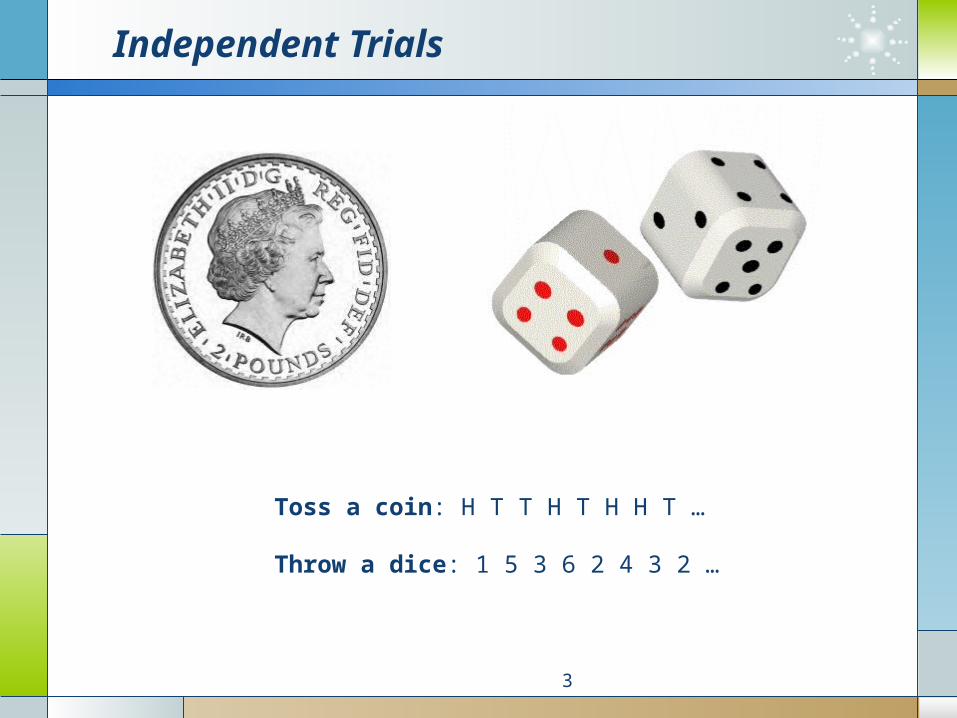
Independent Trials

3

Toss a coin: H T T H T H H T …

Throw a dice: 1 5 3 6 2 4 3 2 …

Sequence of Data

4

Sequence of Data

5

bb

aa

11

ugly is Hellen

pretty is Hellen

ugly is Hellenpretty is Hellen

Deterministic Finite Automaton

Theory of Computation

A finite state machine where for each pair of state and input symbol

there is one and only one transition to a next state

A DFA is a 5-tuple (Q, Σ, δ, q0, F):

A finite set of states (Q)

A finite set of input symbols called the alphabet (Σ)

A transition function (δ : Q × Σ → Q)

A start state (q0 ∈ Q)

A set of accept states (F ⊆ Q)

6

DFA Example

A DFA that determines the number of 0s

M = (Q, Σ, δ, q0, F) where

• Q = {S1, S2},

• Σ = {0, 1},

• q0 = S1,

• F = {S1},

• δ is defined by7

0 1

S1 S2 S1

S2 S1 S2

State Transition Table

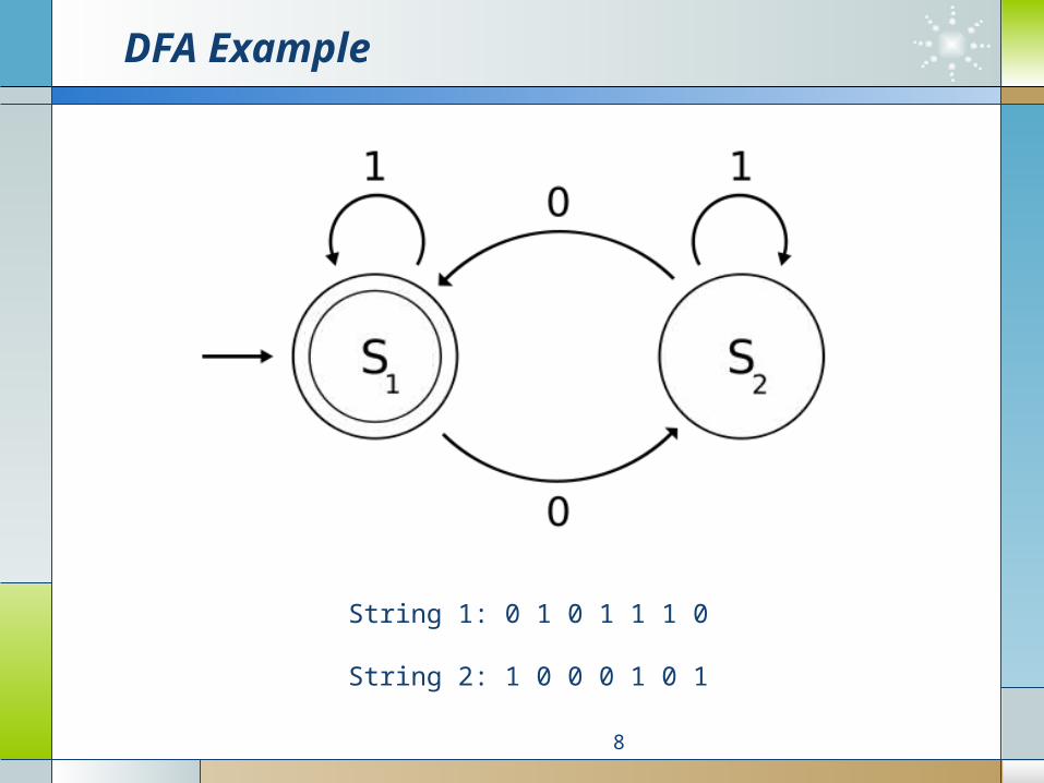
DFA Example

8

String 1: 0 1 0 1 1 1 0

String 2: 1 0 0 0 1 0 1

A Markov System

Has N states: {s1, s2, … , sN}

There are T discrete time steps: t= 1, 2, …, T

On the tth step, the system is on exactly one of the states st.

Between two time steps, the next state is chosen randomly.

The current state determines the probability for the next state.

9

s1

s2 s3

α13

α31

α11

α33

α12

α21α22

α32

α23

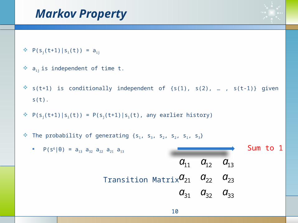
Markov Property

P(sj(t+1)|si(t)) = aij

aij is independent of time t.

s(t+1) is conditionally independent of {s(1), s(2), … , s(t-1)} given s(t).

P(sj(t+1)|si(t)) = P(sj(t+1)|si(t), any earlier history)

The probability of generating {s1, s3, s2, s2, s1, s3}

P(s6|θ) = a13 a32 a22 a21 a13

10

333231

232221

131211

aaa

aaa

aaa

Sum to 1

Transition Matrix

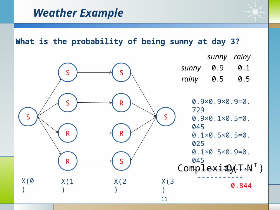
Weather Example

11

Q: What is the probability of being sunny at day 3?

0.9×0.9×0.9=0.7290.9×0.1×0.5=0.0450.1×0.5×0.5=0.0250.1×0.5×0.9=0.045-------------------------

0.844

)NO(T:Complexity T

S

X(0)

S

S

R

R

S

R

R

S

X(1) X(2)

S

X(3)

5050 1090..

..

rainy

sunny

rainysunny

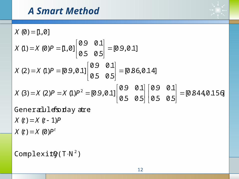
A Smart Method

12

)NO(T :Complexity

)0()(

)1()(

:areday t for rules General

]156.0,844.0[5.05.0

1.09.0

5.05.0

1.09.0]1.0,9.0[)1()2()3(

]14.0,86.0[5.05.0

1.09.0]1.0,9.0[)1()2(

]1.0,9.0[5.05.0

1.09.0]0,1[)0()1(

]0,1[)0(

2

2

tPXtX

PtXtX

PXPXX

PXX

PXX

X

A Smart Method

13

1

0

sunny

rainy

X(0)

0.86

0.14

X(2)

0.9×0.9

0.1×0.5

0.9×0.1

0.1×0.5

0.9

0.1

X(1)

1×0.9

0×0.5

1×0.1

0×0.5

0.844

0.156

0.86×0.9

0.14×0.5

0.86×0.1

0.14×0.5

X(3)

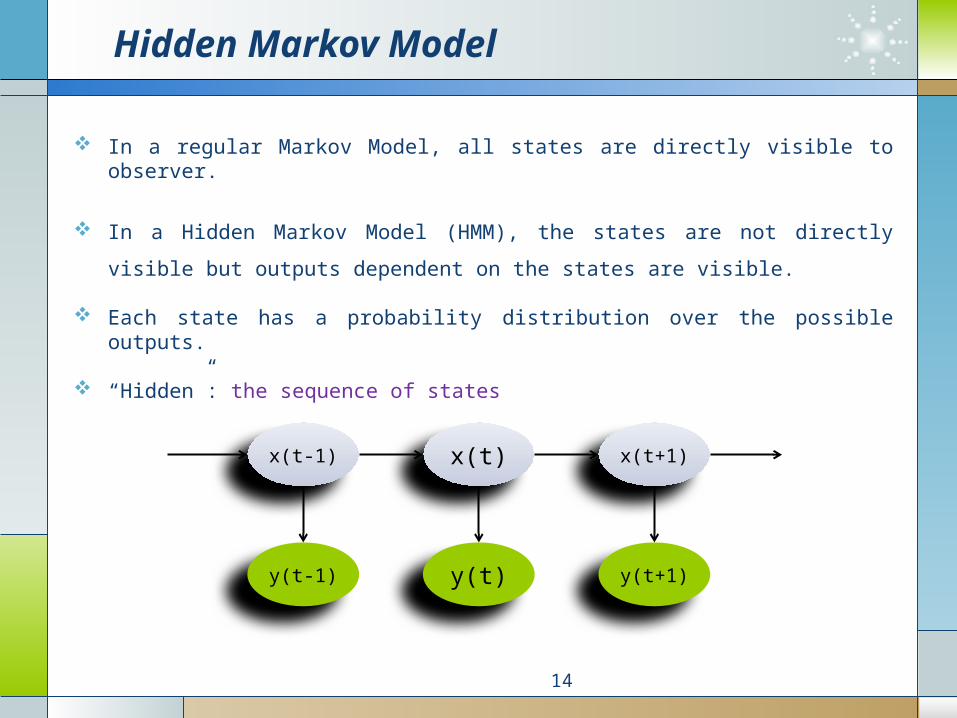
Hidden Markov Model

In a regular Markov Model, all states are directly visible to observer.

In a Hidden Markov Model (HMM), the states are not directly visible but

outputs dependent on the states are visible.

Each state has a probability distribution over the possible outputs.

“Hidden”: the sequence of states

14

x(t-1) x(t) x(t+1)

y(t-1) y(t) y(t+1)

Structure of HMM

15

HMM Demo

16

State Sequences

5 3 2 5 3 2

5 3 1 2 1 2

4 3 2 5 3 2

4 3 1 2 1 2

3 1 2 5 3 2

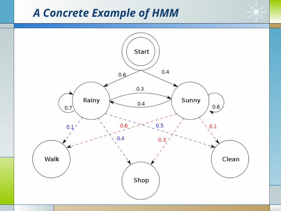
A Concrete Example of HMM

states = {'Rainy', 'Sunny‘}

observations = {'walk', 'shop', 'clean’}

start_probability = {'Rainy': 0.6, 'Sunny': 0.4}

transition_probability = {

'Rainy' : {'Rainy': 0.7, 'Sunny': 0.3},

'Sunny' : {'Rainy': 0.4, 'Sunny': 0.6},

}

emission_probability = {

'Rainy' : {'walk': 0.1, 'shop': 0.4, 'clean': 0.5},

'Sunny' : {'walk': 0.6, 'shop': 0.3, 'clean': 0.1},

}

17

A Concrete Example of HMM

18

Two Canonical Questions

Q1: Given the parameters of the model, compute the probability of a

particular output sequence.

What is the probability of {“walk” “shop” “clean”}?

Q2: Given the parameters of the model and an output sequence, find the

state sequence that is most likely to generate that output sequence.

What is the most likely sequence of rainy/sunny days?

Both questions require calculations over all possible state sequences.

Fortunately, they can be solved more efficiently.

Recall how to smartly calculate P(sj(t)) in a Markov system.

19

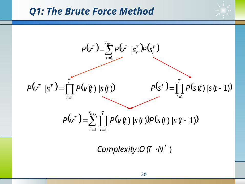
Q1: The Brute Force Method

20

max

1

|r

r

Tr

Tr

TT sPsvPvP

T

t

T tstsPsP1

)1(|)(

T

t

TT tstvPsvP1

)(|)(|

max

1 1

)1(|)()(|)(r

r

T

t

T tstsPtstvPvP

)(: TNTOComplexity

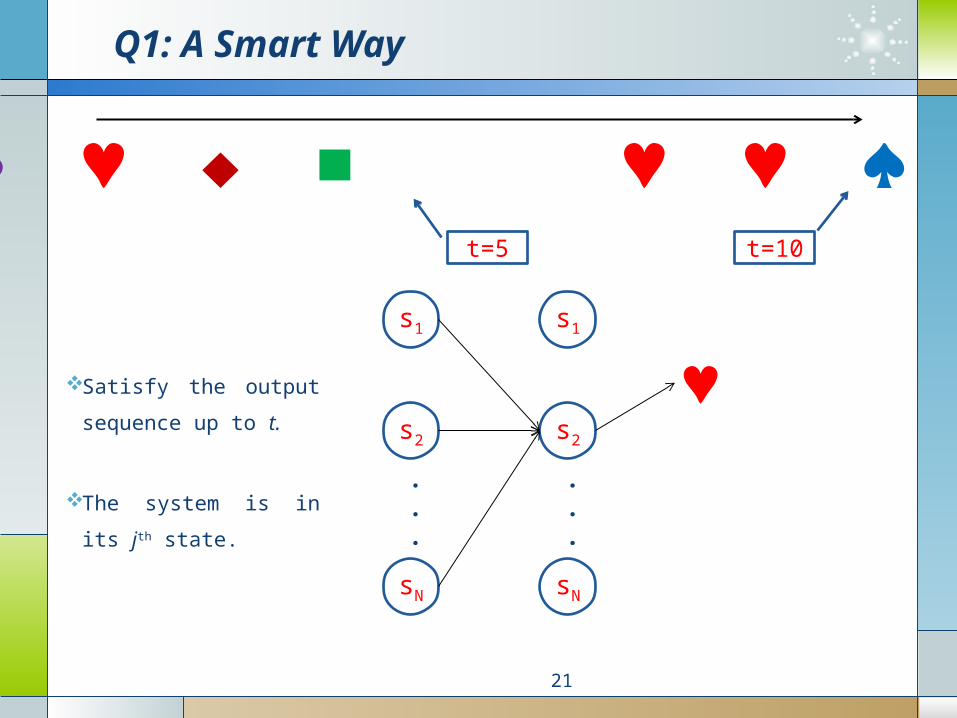
Q1: A Smart Way

21

♠ ♣ ♥ ♦ ■ ♥ ♥ ♠ ♦ ♣t=5 t=10

s1

s2

sN

.

.

.

s1

s2

sN

.

.

.

♥ Satisfy the output

sequence up to t.

The system is in its

jth state.

Q1: A Smart Way

22

)(: 2NTOComplexity

i kjkiji

j

vtvbat

t

)(,)1(

state initialj &0t ,1

state initialj & 0 t ,0

)(

N

i ii αb

vv

1 22222 23 3

)()(

)( Given

jkjkijij svPbtstsPα |)(|)( 1

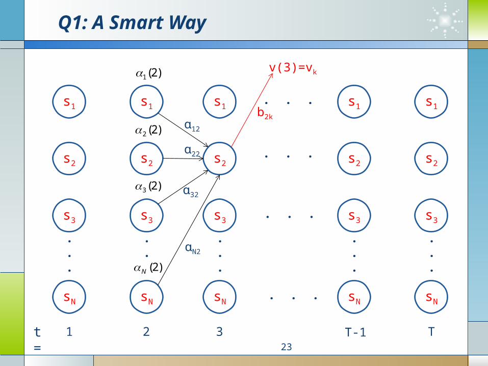
Q1: A Smart Way

23

s1

s2

s3

sN

.

.

.

s1

s2

s3

sN

.

.

s1

s2

s3

sN

.

.

.

s1

s2

s3

sN

.

.

.

s1

s2

s3

sN

.

.

.

. . .

. . .

. . .

. . .

)2(2

)2(1

)2(3

)2(N

1 2 3 TT-1t =

ɑ12

ɑ22

ɑ32

ɑN2

v(3)=vk

b2k

Q1: Example

24

1.00.01.08.0

1.02.05.02.0

4.01.03.02.0

0001

ija

2.01.02.05.00

1.07.01.01.00

2.01.04.03.00

00001

jkb

absorbing state

1)0(

},,,{

1

02314

vvvvv

s0 s1 s2 s3

s0

s1

s2

s3

v0 v1 v2 v3 v4

s0

s1

s2

s3

Q1: Example

25

0

1

0

0

0

.09

.01

.2

0

.0052

.0077

.0057

0

.0024

.0002

.0007

.0011

0

0

0

s0

s1

s2

s3

1 32 40t=

v1 v3 v2 v0

0.2×0

0.3×0.3

0.1×0.1

0.4×0.5

Q1: Example

26

0

1

0

0

0

.09

.01

.2

0

.0052

.0077

.0057

0

.0024

.0002

.0007

.0011

0

0

0

s0

s1

s2

s3

1 32 40t=

v1 v3 v2 v0

×0

×0.3

×0.5

×0.1

×0.1

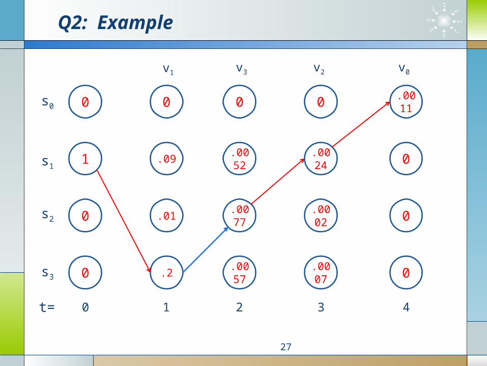
Q2: Example

27

0

1

0

0

0

.09

.01

.2

0

.0052

.0077

.0057

0

.0024

.0002

.0007

.0011

0

0

0

s0

s1

s2

s3

1 32 40t=

v1 v3 v2 v0

28

10 Minutes …

Decision Making

29

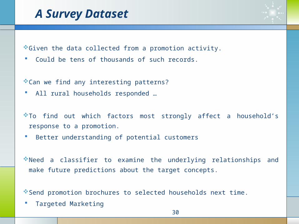
A Survey Dataset

Given the data collected from a promotion activity.

Could be tens of thousands of such records.

Can we find any interesting patterns?

All rural households responded …

To find out which factors most strongly affect a household’s response to a

promotion.

Better understanding of potential customers

Need a classifier to examine the underlying relationships and make future

predictions about the target concepts.

Send promotion brochures to selected households next time.

Targeted Marketing 30

A Survey Dataset

District House Type IncomePrevious Customer

Outcome

Suburban Detached High No Nothing

Suburban Detached High Yes Nothing

Rural Detached High No Responded

Urban Semi-detached High No Responded

Urban Semi-detached Low No Responded

Urban Semi-detached Low Yes Nothing

Rural Semi-detached Low Yes Responded

Suburban Terrace High No Nothing

Suburban Semi-detached Low No Responded

Urban Terrace Low No Responded

Suburban Terrace Low Yes Responded

Rural Terrace High Yes Responded

Rural Detached Low No Responded

Urban Terrace High Yes Nothing

31

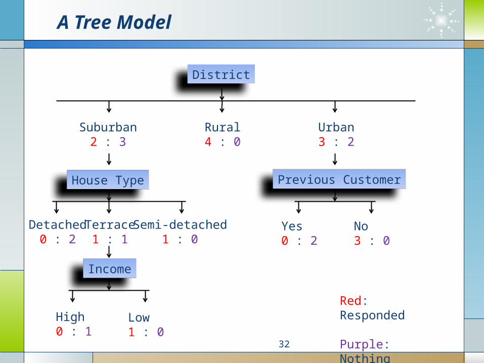
A Tree Model

32

District

Suburban2 : 3

Rural4 : 0

Urban3 : 2

House Type

Detached0 : 2

Semi-detached1 : 0

Terrace1 : 1

Income

High0 : 1

Low1 : 0

Red: Responded

Purple: Nothing

Previous Customer

Yes0 : 2

No3 : 0

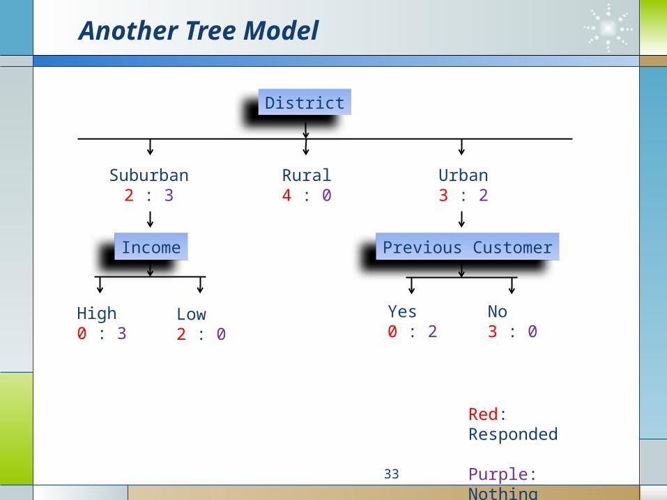
Another Tree Model

33

District

Suburban2 : 3

Rural4 : 0

Urban3 : 2

Income

High0 : 3

Low2 : 0

Previous Customer

Yes0 : 2

No3 : 0

Red: Responded

Purple: Nothing

Some Notes …

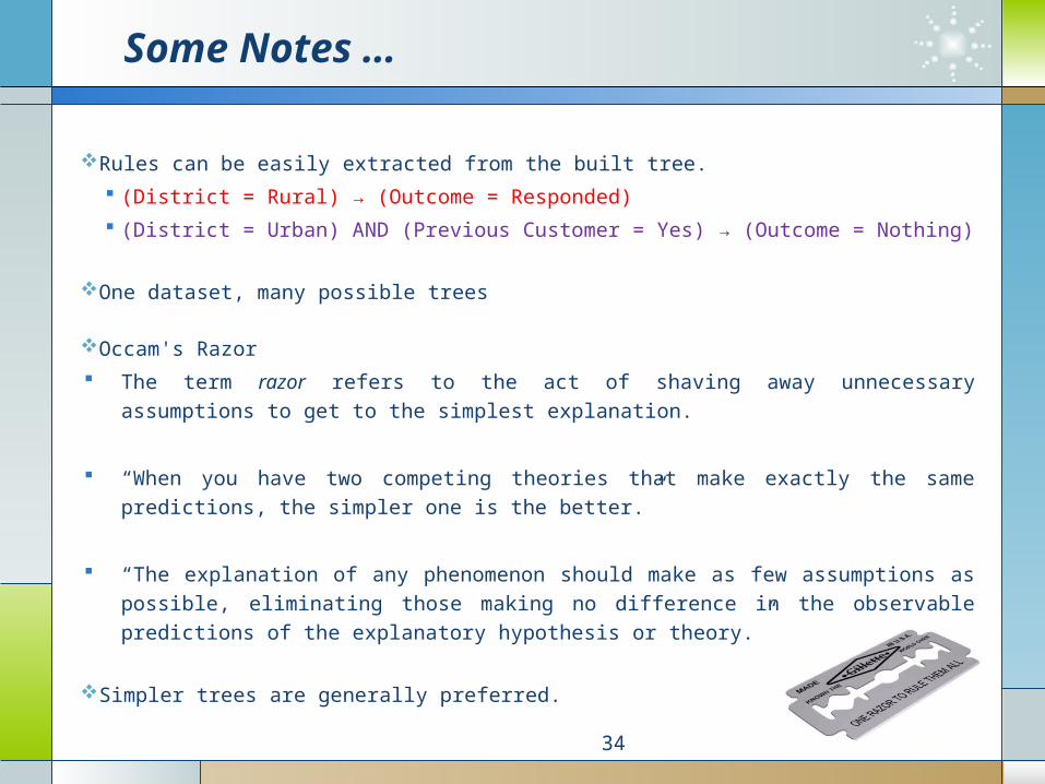
Rules can be easily extracted from the built tree.

(District = Rural) → (Outcome = Responded)

(District = Urban) AND (Previous Customer = Yes) → (Outcome = Nothing)

One dataset, many possible trees

Occam's Razor

The term razor refers to the act of shaving away unnecessary assumptions to

get to the simplest explanation.

“When you have two competing theories that make exactly the same

predictions, the simpler one is the better.”

“The explanation of any phenomenon should make as few assumptions as

possible, eliminating those making no difference in the observable predictions

of the explanatory hypothesis or theory.”

Simpler trees are generally preferred. 34

ID3

How to build a shortest tree from a dataset?

Iterative Dichotomizer 3

Ross Quinlan: http://www.rulequest.com/

One of the most influential Decision Trees models

Top-down, greedy search through the space of possible decision trees

Since we want to construct short trees …

It is better to put certain attributes higher up the tree.

Some attributes split the data more purely than others.

Their values correspond more consistently with the class labels.

Need to have some sort of measure to compare candidate attributes.

35

Entropy

36

C

iii ppSEntropy

1

)log()(

pi: the proportion of instances in the dataset that take the i th target value

)] ( 14/5 ),( 14/9[ responsesnoresponsesS

940.014

5log

14

5

14

9log

14

9)( 22 SEntropy

Av

vv SEntropyS

SSEntropyASGain )(

||

||)(),(

Sv is the subset of S where the attribute A takes the value v.

Attribute Selection

37

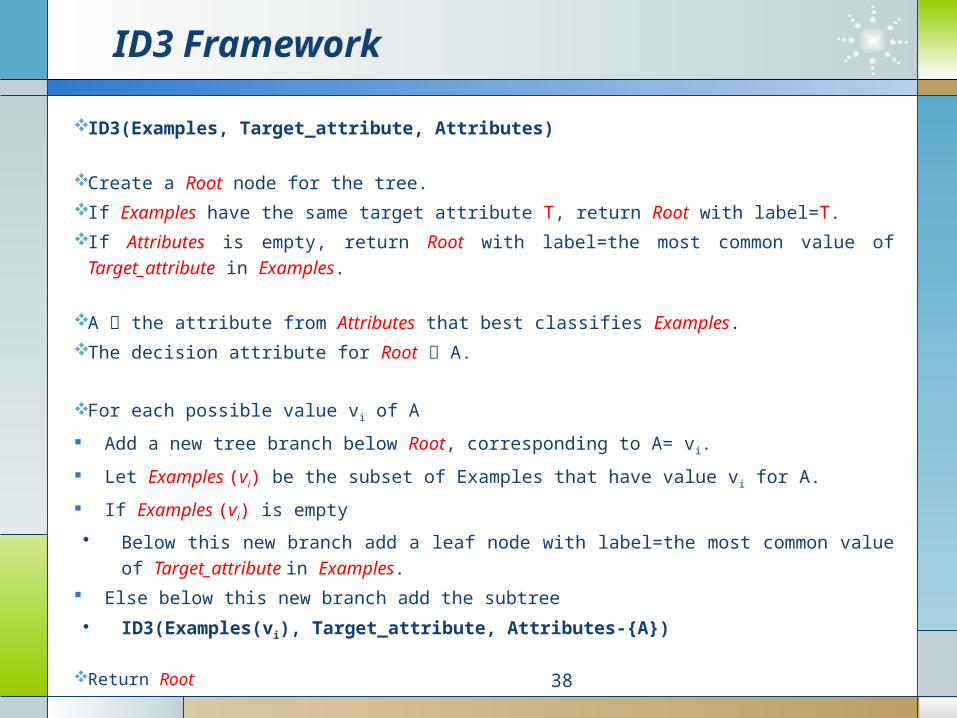
ID3 Framework

ID3(Examples, Target_attribute, Attributes)

Create a Root node for the tree.

If Examples have the same target attribute T, return Root with label=T.

If Attributes is empty, return Root with label=the most common value of Target_attribute in Examples.

A the attribute from Attributes that best classifies Examples.

The decision attribute for Root A.

For each possible value vi of A

Add a new tree branch below Root, corresponding to A= vi.

Let Examples (vi) be the subset of Examples that have value vi for A.

If Examples (vi) is empty

• Below this new branch add a leaf node with label=the most common value of

Target_attribute in Examples.

Else below this new branch add the subtree

• ID3(Examples(vi), Target_attribute, Attributes-{A})

Return Root38

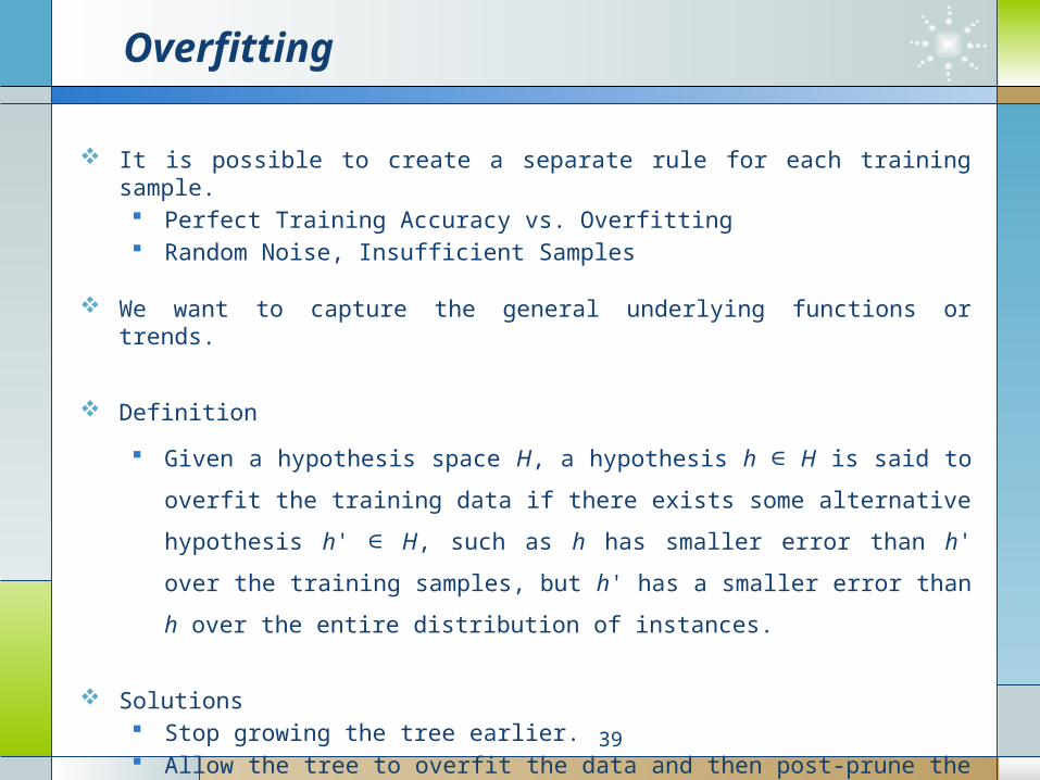
Overfitting

It is possible to create a separate rule for each training sample. Perfect Training Accuracy vs. Overfitting Random Noise, Insufficient Samples

We want to capture the general underlying functions or trends.

Definition

Given a hypothesis space H, a hypothesis h ∈ H is said to overfit the training

data if there exists some alternative hypothesis h' ∈ H, such as h has smaller

error than h' over the training samples, but h' has a smaller error than h over

the entire distribution of instances.

Solutions Stop growing the tree earlier. Allow the tree to overfit the data and then post-prune the tree.

39

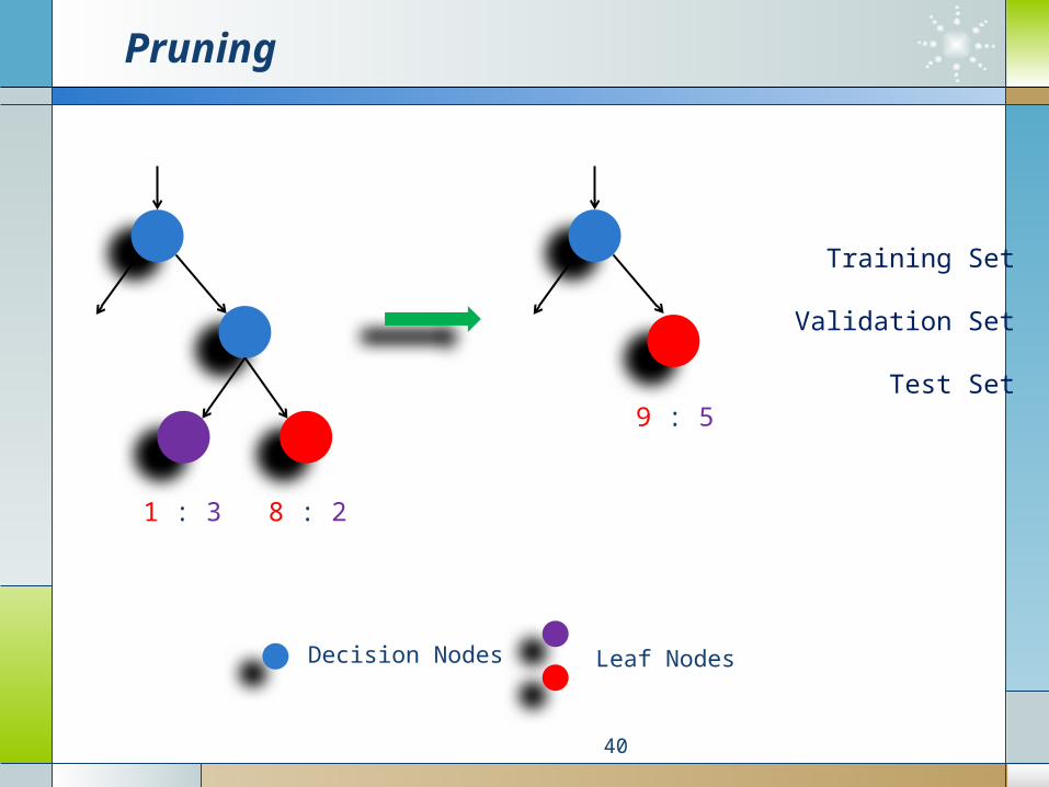
Pruning

40

Decision Nodes Leaf Nodes

1 : 3 8 : 2

9 : 5

Training Set

Validation Set

Test Set

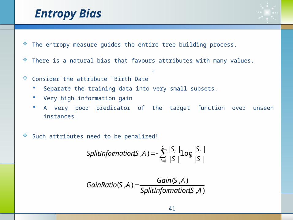
Entropy Bias

The entropy measure guides the entire tree building process.

There is a natural bias that favours attributes with many values.

Consider the attribute “Birth Date”

Separate the training data into very small subsets.

Very high information gain

A very poor predicator of the target function over unseen instances.

Such attributes need to be penalized!

41

||

||log

||

||),( 2

1 S

S

S

SASmationSplitInfor i

C

i

i

),(

),(),(

ASmationSplitInfor

ASGainASGainRatio

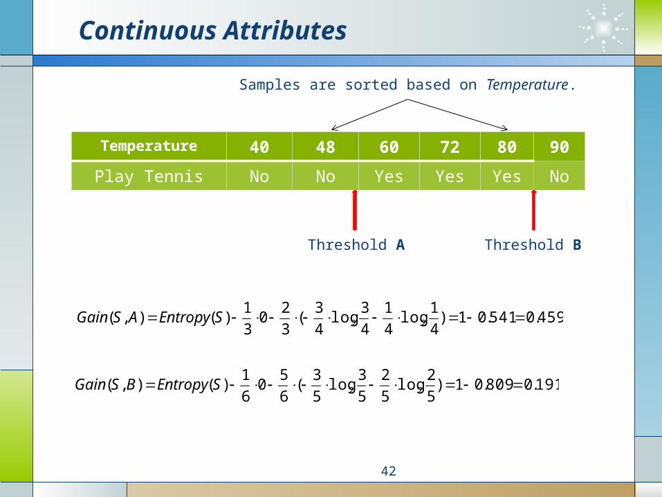
Continuous Attributes

42

Temperature 40 48 60 72 80 90

Play Tennis No No Yes Yes Yes No

Threshold A Threshold B

Samples are sorted based on Temperature.

459.0541.01)4

1log

4

1

4

3log

4

3(

3

20

3

1)(),( 22 SEntropyASGain

191.0809.01)5

2log

5

2

5

3log

5

3(

6

50

6

1)(),( 22 SEntropyBSGain

Reading Materials

Text Book (HMM) Richard O. Duda et al., Pattern Classification, Chapter 3.10, John Wiley & Sons Inc.

Text Book (DT) Tom Mitchell, Machine Learning, Chapter 3, McGraw-Hill.

Online Tutorial (HMM) http://www.comp.leeds.ac.uk/roger/HiddenMarkovModels/html_dev/main.html

http://www.bioss.ac.uk/~dirk/talks/urfer02_hmm.pdf

Online Tutorial (DT) http://www.decisiontrees.net/node/21 (with interactive demos)

http://www.autonlab.org/tutorials/dtree18.pdf

http://people.revoledu.com/kardi/tutorial/DecisionTree/index.html

http://www.public.asu.edu/~kirkwood/DAStuff/decisiontrees/index.html

Wikipedia & Google43

Review

What is a Markov system?

What is a hidden Markov system?

What are the two canonical questions in HMM?

What is a Decision Tree model?

What is Occam’s Razor?

What is information entropy?

How to use information entropy in DT?

What is the main issue with information entropy?

Why and how to do pruning in DT?

How to handle continuous attributes in DT?44

Next Week’s Class Talk

Volunteers are required for next week’s class talk.

Topic 1: C4.5 Algorithm

Topic 2: CART

Hints:

Both are advanced DT models.

How to select attributes?

How to handle continuous attributes?

How to handle missing values?

What else can they do?

Length: 20 minutes plus question time

45