Logistic Regression: Interaction Terms - · PDF fileInteractions in Logistic Regression I For...
23
Logistic Regression: Interaction Terms 1
Transcript of Logistic Regression: Interaction Terms - · PDF fileInteractions in Logistic Regression I For...

Logistic Regression: Interaction Terms
1
Interactions in Logistic Regression
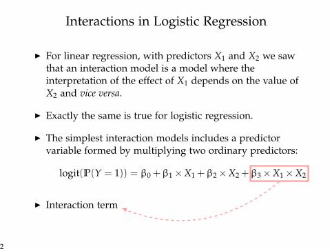
I For linear regression, with predictors X1 and X2 we sawthat an interaction model is a model where theinterpretation of the effect of X1 depends on the value ofX2 and vice versa.
I Exactly the same is true for logistic regression.
I The simplest interaction models includes a predictorvariable formed by multiplying two ordinary predictors:
logit(P(Y = 1)) = β0 +β1 ×X1 +β2 ×X2 +β3 ×X1 ×X2
I Interaction term
2

Interactions in Logistic Regression
We will look at the interpretation of interactions in 3 cases:
1 Interaction between two dummy variables.
2 Interaction between a dummy and a continuous variable.
3 Interaction between two continuous variables.
3

Interaction Between 2 Dummy Variables
I Consider a logistic model for the risk of suffering a heartattack over a year in terms gender and smoking status:
logit P(Y = 1) = β0 +β1sex+β2smoke+β3(sex× smoke)
I sex indicates gender (male=1, female=0)
I smoke indicates smoking status (smokes=1, does not=0).
4
Interpreting the Intercept
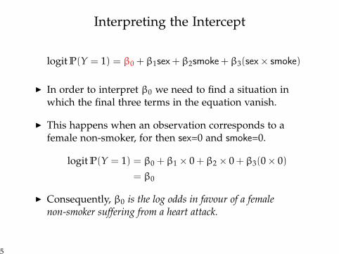
logit P(Y = 1) = β0 +β1sex+β2smoke+β3(sex× smoke)
I In order to interpret β0 we need to find a situation inwhich the final three terms in the equation vanish.
I This happens when an observation corresponds to afemale non-smoker, for then sex=0 and smoke=0.
logit P(Y = 1) = β0 +β1 × 0 +β2 × 0 +β3(0 × 0)= β0
I Consequently, β0 is the log odds in favour of a femalenon-smoker suffering from a heart attack.
5
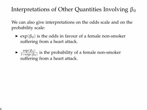
Interpretations of Other Quantities Involving β0
We can also give interpretations on the odds scale and on theprobability scale:
I exp(β0) is the odds in favour of a female non-smokersuffering from a heart attack.
I exp(β0)1+exp(β0)
is the probability of a female non-smokersuffering from a heart attack.
6
Interpreting β1 and β2
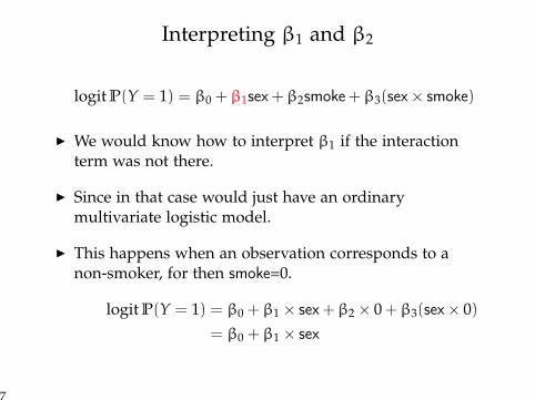
logit P(Y = 1) = β0 +β1sex+β2smoke+β3(sex× smoke)
I We would know how to interpret β1 if the interactionterm was not there.
I Since in that case would just have an ordinarymultivariate logistic model.
I This happens when an observation corresponds to anon-smoker, for then smoke=0.
logit P(Y = 1) = β0 +β1 × sex+β2 × 0 +β3(sex× 0)= β0 +β1 × sex
7

Interpreting β1 and β2
I Amongst non-smokers
logit P(Y = 1) = β0 +β1 × sex
I We know how to interpret β1 in this case as its aunivariate logistic model.
I β1 is the log-odds ratio comparing males and femalesamongst non-smokers.
I exp(β1) is the odds ratio comparing males and femalesamongst non-smokers.
8
Interpreting β1 and β2
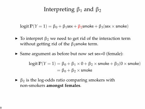
logit P(Y = 1) = β0 +β1sex+β2smoke+β3(sex× smoke)
I To interpret β2 we need to get rid of the interaction termwithout getting rid of the β2smoke term.
I Same argument as before but now set sex=0 (female):
logit P(Y = 1) = β0 +β1 × 0 +β2 × smoke+β3(0 × smoke)= β0 +β2 × smoke
I β2 is the log-odds ratio comparing smokers withnon-smokers amongst females.
9

Interpreting β3
logit P(Y = 1) = β0 +β1sex+β2smoke+β3(sex× smoke)
I To interpret β3 rewrite the regression equation:
logit P(Y = 1) = β0 + [β1 +β3smoke]sex+β2smoke
I This looks like a multivariate regression model with sexand smoke as predictors where:
I β1 +β3smoke is the log-odds ratio for males vs. females;I β2 is the log odds ratio for smokers vs. non-smokers.
I β3 is the difference between the log-odds ratio comparingmales vs females in smokers and the log-odds ratiocomparing males vs. females in non-smokers.
10

Interpreting β3
logit P(Y = 1) = β0 +β1sex+β2smoke+β3(sex× smoke)
I We could just as well have rewritten the equation this way:
logit P(Y = 1) = β0 +β1sex+ [β2 +β3sex]smoke
I β3 is the difference between the log-odds ratio comparingsmokers vs non-smokers in males and the log-odds ratiocomparing smokers vs. non-smokers in females.
I So we have two ways of thinking about β3:1 either as modification of the effect of smoke by sex2 or the modification of the effect of sex by smoke.
11

Quick Lookup Table
We can draw up a table for the 4 types of observation:
sex smoke logit(P(Y = 1))
1 Male Yes β0 +β1 +β2 +β3
2 Male No β0 +β1
3 Female Yes β0 +β2
4 Female No β0
I This allows us to find the function of the parameterscorresponding to a log-odds ratio and vice versa.
I e.g. 3 - 4 shows us that the log-odds ratio for smokersvs. non-smokers amongst females is β2
I e.g. 1 - 2 shows us that the log-odds ratio for smokersvs. non-smokers amongst males is β2 +β3
I Note β3 is the difference of these two log odds ratios.
12

Interaction Between a Dummy Variable and aContinuous Variable
I Consider a logistic model where the main predictors aresex (a dummy coded as before) and age (in years)
logit P(Y = 1) = β0 +β1sex+β2age+β3(sex× age)
I β0 is the log-odds in favour of a female age 0 sufferingfrom a heart attack.
13
Interaction Between a Dummy Variable and aContinuous Variable
I Consider a logistic model where the main predictors aresex (a dummy coded as before) and age (in years)
logit P(Y = 1) = β0 +β1sex+β2age+β3(sex× age)
I β1 is the log-odds ratio for males vs. females amongstpeople of age 0.
14
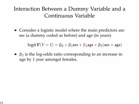
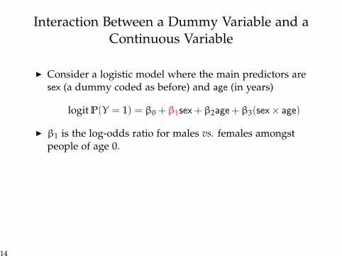
Interaction Between a Dummy Variable and aContinuous Variable
I Consider a logistic model where the main predictors aresex (a dummy coded as before) and age (in years)
logit P(Y = 1) = β0 +β1sex+β2age+β3(sex× age)
I β2 is the log-odds ratio corresponding to an increase inage by 1 year amongst females.
15

Interaction Between a Dummy Variable and aContinuous Variable
I Consider a logistic model where the main predictors aresex (a dummy coded as before) and age (in years)
logit P(Y = 1) = β0 +β1sex+β2age+β3(sex× age)
I β3 is the difference between the log-odds ratiocorresponding to a change in age by 1 year amongst malesand the the log-odds ratio corresponding to an increase inage by 1 year amongst females.
I β3 is also difference between the log-odds ratios for malesvs. females in two age homogenous groups which differby 1 year.
16
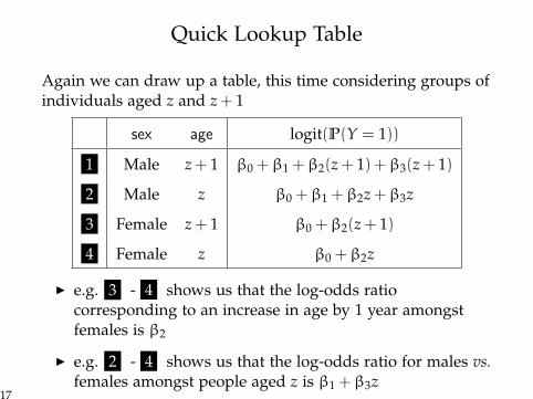
Quick Lookup Table
Again we can draw up a table, this time considering groups ofindividuals aged z and z + 1
sex age logit(P(Y = 1))
1 Male z + 1 β0 +β1 +β2(z + 1) +β3(z + 1)
2 Male z β0 +β1 +β2z +β3z
3 Female z + 1 β0 +β2(z + 1)
4 Female z β0 +β2z
I e.g. 3 - 4 shows us that the log-odds ratiocorresponding to an increase in age by 1 year amongstfemales is β2
I e.g. 2 - 4 shows us that the log-odds ratio for males vs.females amongst people aged z is β1 +β3z
17
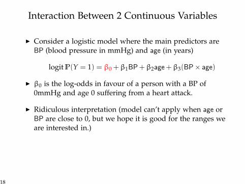
Interaction Between 2 Continuous Variables
I Consider a logistic model where the main predictors areBP (blood pressure in mmHg) and age (in years)
logit P(Y = 1) = β0 +β1BP+β2age+β3(BP× age)
I β0 is the log-odds in favour of a person with a BP of0mmHg and age 0 suffering from a heart attack.
I Ridiculous interpretation (model can’t apply when age orBP are close to 0, but we hope it is good for the ranges weare interested in.)
18

Interaction Between 2 Continuous Variables
I Consider a logistic model where the main predictors areBP (blood pressure in mmHg) and age (in years)
logit P(Y = 1) = β0 +β1BP+β2age+β3(BP× age)
I β1 is the log-odds ratio corresponding to an increase in BPby 1mmHg amongst people aged 0.
19
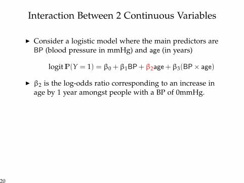
Interaction Between 2 Continuous Variables
I Consider a logistic model where the main predictors areBP (blood pressure in mmHg) and age (in years)
logit P(Y = 1) = β0 +β1BP+β2age+β3(BP× age)
I β2 is the log-odds ratio corresponding to an increase inage by 1 year amongst people with a BP of 0mmHg.
20
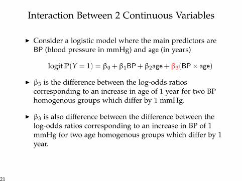
Interaction Between 2 Continuous Variables
I Consider a logistic model where the main predictors areBP (blood pressure in mmHg) and age (in years)
logit P(Y = 1) = β0 +β1BP+β2age+β3(BP× age)
I β3 is the difference between the log-odds ratioscorresponding to an increase in age of 1 year for two BPhomogenous groups which differ by 1 mmHg.
I β3 is also difference between the difference between thelog-odds ratios corresponding to an increase in BP of 1mmHg for two age homogenous groups which differ by 1year.
21

Quick Lookup Table
Again we can draw up a table, this time consideringindividuals with BP w and w + 1 and aged z and z + 1
BP age logit(P(Y = 1))
1 w + 1 z + 1 β0 +β1(w + 1) +β2(z + 1) +β3(w + 1)(z + 1)
2 w + 1 z β0 +β1(w + 1) +β2z +β3(w + 1)z
3 w z + 1 β0 +β1w +β2(z + 1) +β3w(z + 1)
4 w z β0 +β1w +β2z +β3wz
I e.g. 3 - 4 shows us that the log-odds ratiocorresponding to an increase in age by 1 year amongstthose of BP w is β2 +β3w.
I e.g. 2 - 4 shows us that the log-odds ratiocorresponding to an increase in BP by 1 mmHg amongstthose of age z is β1 +β3z.
22
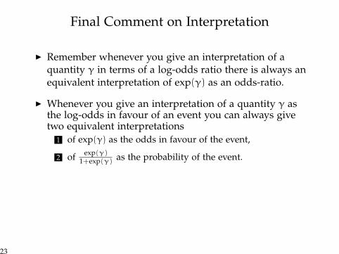
Final Comment on Interpretation
I Remember whenever you give an interpretation of aquantity γ in terms of a log-odds ratio there is always anequivalent interpretation of exp(γ) as an odds-ratio.
I Whenever you give an interpretation of a quantity γ asthe log-odds in favour of an event you can always givetwo equivalent interpretations
1 of exp(γ) as the odds in favour of the event,
2 of exp(γ)1+exp(γ) as the probability of the event.
23