Logistic

IntroductionProbability, Odds, and Odds Ratios

Logistic RegressionROC Curves

SAS Logistic Regression

Jason Brinkley - Department of Biostatistics

February 2, 2009

Jason Brinkley - Department of Biostatistics SAS Logistic Regression



Traditional Regression

I In traditional multiple regression, the intent is to studywhat effect different covariates have on a quantitativeresponse.

I There are many scenarios when the main question ofinterest involves a dichotomous response: Yes/No,Success/Fail, Sick/Well, etc.

I Traditional methods fail to adequately model this kind ofdata, let’s look at an example.




Accident Data

I (From Cody) Let’s say we want to see if age, visionstatus, driver education, and gender can be used topredict whether a person had an accident in the past year.

I Consider a sample of such individuals (see the website forrelated files).

I So we can import the data from Excel using the ProcImport statement.




SAS> PROC IMPORT OUT= WORK.ACCIDENT

SAS> DATAFILE= "U:\SAS Workshop\Lecture 3 - Linear and Logistic Regression\Cody\accident.xls"

SAS> DBMS=EXCEL REPLACE;

SAS> RANGE="accident$";

SAS> GETNAMES=YES;

SAS> MIXED=NO;

SAS> SCANTEXT=YES;

SAS> USEDATE=YES;

SAS> SCANTIME=YES;

SAS> RUN;

SAS>

SAS> PROC FORMAT;

SAS>

SAS> VALUE VISION 0 = ’No Problem’

SAS> 1 = ’Some Problem’;

SAS> VALUE YES_NO 0 = ’No’

SAS> 1 = ’Yes’;

SAS> RUN;




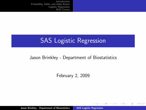
SAS> DATA LOGISTIC;

SAS>

SAS> Set Accident;

SAS>

SAS> LABEL

SAS> ACCIDENT = ’Accident in Last Year?’

SAS> AGE = ’Age of Driver’

SAS> VISION = ’Vision Problem?’

SAS> DRIVER_ED = ’Driver Education?’;

SAS> FORMAT ACCIDENT DRIVER_ED YES_NO.

SAS> VISION VISION.;

SAS> RUN;




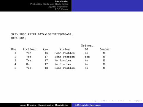
SAS> PROC PRINT DATA=LOGISTIC(OBS=5);

SAS> RUN;

Driver_

Obs Accident Age Vision Ed Gender

1 Yes 16 Some Problem No M

2 Yes 17 Some Problem Yes M

3 Yes 17 No Problem No M

4 No 17 No Problem No M

5 Yes 18 Some Problem No M




Graph Age Versus Accident

SAS> PROC GPLOT;

SAS> PLOT ACCIDENT*AGE;

SAS> RUN;




I Just by examining the graph we can see why traditionalmodels will fail here.

I What we are really interested in is whether age, visionstatus, driver education, and gender have an impact onthe PROBABILITY of an accident.

I Since what are really interested in is modelingprobabilities different techniques need to be used.




Probability and Odds

I Logistic regression is a good way to model this type ofdata, in order to understand this type of regression weshould first talk about odds and odds ratios.

I Let’s say P is the probability of an accident, then theodds of having an accident are given by

Odds =P

1− P

I Sometimes we will find it important to go from odds backto probabilities so also note

P =Odds

1 + Odds.Jason Brinkley - Department of Biostatistics SAS Logistic Regression



Odds Ratios

I To compare the odds of having an accident betweendifferent groups (i.e. different genders or different visionproblems) we often use odds ratios.

I Say the chance of having a wreck among people withpoor vision is 30% and among people with good visionit’s 10%. The corresponding odds are 0.43 and 0.11, theratio of the odds is 3.91. So the odds of an accident havealmost quadrupled for people with poor vision problems.

I Odds and odds ratios are easier to work withmathematically than pure probabilities, especially in thescenarios where you have a rare event.




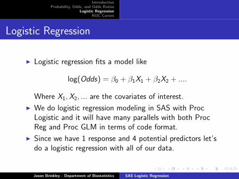
Logistic Regression

I Logistic regression fits a model like

log(Odds) = β0 + β1X1 + β2X2 + ....

Where X1,X2, ... are the covariates of interest.

I We do logistic regression modeling in SAS with ProcLogistic and it will have many parallels with both ProcReg and Proc GLM in terms of code format.

I Since we have 1 response and 4 potential predictors let’sdo a logistic regression with all of our data.




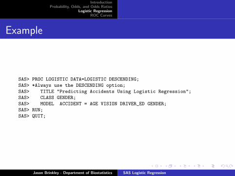
Example

SAS> PROC LOGISTIC DATA=LOGISTIC DESCENDING;

SAS> *Always use the DESCENDING option;

SAS> TITLE "Predicting Accidents Using Logistic Regression";

SAS> CLASS GENDER;

SAS> MODEL ACCIDENT = AGE VISION DRIVER_ED GENDER;

SAS> RUN;

SAS> QUIT;




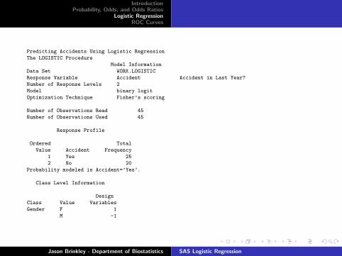
Predicting Accidents Using Logistic Regression

The LOGISTIC Procedure

Model Information

Data Set WORK.LOGISTIC

Response Variable Accident Accident in Last Year?

Number of Response Levels 2

Model binary logit

Optimization Technique Fisher’s scoring

Number of Observations Read 45

Number of Observations Used 45

Response Profile

Ordered Total

Value Accident Frequency

1 Yes 25

2 No 20

Probability modeled is Accident=’Yes’.

Class Level Information

Design

Class Value Variables

Gender F 1

M -1




Model Convergence Status

Convergence criterion (GCONV=1E-8) satisfied.

Model Fit Statistics

Intercept

Intercept and

Criterion Only Covariates

AIC 63.827 59.094

SC 65.633 68.128

-2 Log L 61.827 49.094



Testing Global Null Hypothesis: BETA=0

Test Chi-Square DF Pr > ChiSq

Likelihood Ratio 12.7321 4 0.0127

Score 11.4432 4 0.0220

Wald 9.0132 4 0.0608

Type 3 Analysis of Effects

Wald

Effect DF Chi-Square Pr > ChiSq

Age 1 0.0170 0.8962

Vision 1 5.4891 0.0191

Driver_Ed 1 5.0776 0.0242

Gender 1 1.0270 0.3109




Analysis of Maximum Likelihood Estimates

Standard Wald

Parameter DF Estimate Error Chi-Square Pr > ChiSq

Intercept 1 0.1373 1.0548 0.0169 0.8965

Age 1 0.00247 0.0190 0.0170 0.8962

Vision 1 1.6758 0.7153 5.4891 0.0191

Driver_Ed 1 -1.7160 0.7615 5.0776 0.0242

Gender F 1 0.3847 0.3796 1.0270 0.3109

Odds Ratio Estimates

Point 95% Wald

Effect Estimate Confidence Limits

Age 1.002 0.966 1.040

Vision 5.343 1.315 21.709

Driver_Ed 0.180 0.040 0.800

Gender F vs M 2.158 0.487 9.559



Association of Predicted Probabilities and Observed Responses

Percent Concordant 77.6 Somers’ D 0.566

Percent Discordant 21.0 Gamma 0.574

Percent Tied 1.4 Tau-a 0.286

Pairs 500 c 0.783




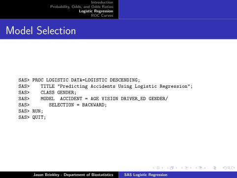
Model Selection



SAS> CLASS GENDER;

SAS> MODEL ACCIDENT = AGE VISION DRIVER_ED GENDER/

SAS> SELECTION = BACKWARD;

SAS> RUN;

SAS> QUIT;






Summary of Backward Elimination

Effect Number Wald Variable

Step Removed DF In Chi-Square Pr > ChiSq Label

1 Age 1 3 0.0170 0.8962 Age of Driver

2 Gender 1 2 1.1313 0.2875 Gender


Wald


Vision 1 5.9113 0.0150

Driver_Ed 1 4.5440 0.0330


Standard Wald


Intercept 1 0.1110 0.5457 0.0414 0.8389

Vision 1 1.7137 0.7049 5.9113 0.0150

Driver_Ed 1 -1.5000 0.7037 4.5440 0.0330


Point 95% Wald


Vision 5.550 1.394 22.093

Driver_Ed 0.223 0.056 0.886

Association of Predicted Probabilities and Observed Responses

Percent Concordant 67.2 Somers’ D 0.532

Percent Discordant 14.0 Gamma 0.655

Percent Tied 18.8 Tau-a 0.269

Pairs 500 c 0.766




Age is not significant?

I Our regression models seem to indicate that age is not asignificant covariate, this seems counter intuitive. Let’sexplore the data.

SAS> OPTIONS PS=24;

SAS> PATTERN COLOR=BLACK VALUE=EMPTY;

SAS> PROC GCHART DATA=LOGISTIC;

SAS> TITLE "Distribution of Ages by Accident Status";

SAS> VBAR AGE / MIDPOINTS=10 TO 90 BY 10

SAS> GROUP=ACCIDENT;

SAS> RUN;




FREQUENCY

0

1

2

3

4

5

6

7

8

Age of Driver

Accident in Last Year?No Yes

102030405060708090

102030405060708090




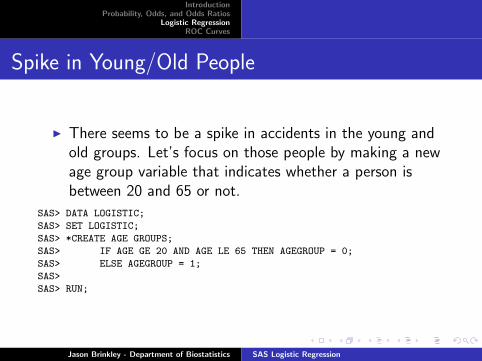
Spike in Young/Old People

I There seems to be a spike in accidents in the young andold groups. Let’s focus on those people by making a newage group variable that indicates whether a person isbetween 20 and 65 or not.

SAS> DATA LOGISTIC;

SAS> SET LOGISTIC;

SAS> *CREATE AGE GROUPS;

SAS> IF AGE GE 20 AND AGE LE 65 THEN AGEGROUP = 0;

SAS> ELSE AGEGROUP = 1;

SAS>

SAS> RUN;




Model Selection



SAS> *THIS NEXT LINE CHANGES THE REFERENCE GROUP;

SAS> CLASS GENDER (PARAM=REF REF=’F’);

SAS> MODEL ACCIDENT = AGEGROUP VISION DRIVER_ED GENDER /

SAS> SELECTION=BACKWARD;

SAS> RUN;

SAS> QUIT;




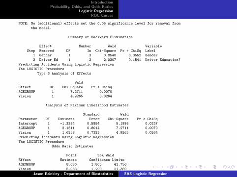
NOTE: No (additional) effects met the 0.05 significance level for removal from

the model.

Summary of Backward Elimination

Effect Number Wald Variable

Step Removed DF In Chi-Square Pr > ChiSq Label

1 Gender 1 3 0.8548 0.3552 Gender

2 Driver_Ed 1 2 2.0307 0.1541 Driver Education?




Wald


AGEGROUP 1 7.2711 0.0070

Vision 1 4.9265 0.0264


Standard Wald


Intercept 1 -1.3334 0.5854 5.1886 0.0227

AGEGROUP 1 2.1611 0.8014 7.2711 0.0070

Vision 1 1.6258 0.7325 4.9265 0.0264




Point 95% Wald


AGEGROUP 8.680 1.805 41.756

Vision 5.083 1.209 21.359




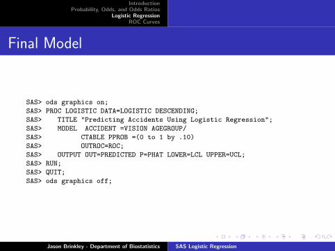
Final Model

SAS> ods graphics on;



SAS> MODEL ACCIDENT =VISION AGEGROUP/

SAS> CTABLE PPROB =(0 to 1 by .10)

SAS> OUTROC=ROC;

SAS> OUTPUT OUT=PREDICTED P=PHAT LOWER=LCL UPPER=UCL;

SAS> RUN;

SAS> QUIT;

SAS> ods graphics off;




Predicted Probabilities

I From our final model we can output a new dataset thatwill have our original data and our predicted probabilites.

SAS> PROC PRINT DATA=PREDICTED(OBS=5);

SAS> TITLE ’Predicted Probabilities and 95% Confidence Limits’;

SAS> RUN;

D

A r A

c i G _

c V v G E L

i i e e G E

d s r n R V P

O e A i _ d O E H L U

b n g o E e U L A C C

s t e n d r P _ T L L

1 Yes 16 Some Problem No M 1 Yes 0.92082 0.70197 0.98288

2 Yes 17 Some Problem Yes M 1 Yes 0.92082 0.70197 0.98288

3 Yes 17 No Problem No M 1 Yes 0.69586 0.36264 0.90197

4 No 17 No Problem No M 1 Yes 0.69586 0.36264 0.90197

5 Yes 18 Some Problem No M 1 Yes 0.92082 0.70197 0.98288




Assessing your models fit and prediction ability

I While there does exist a generalized R square measure forthese types of models, it is not used in general practice.

I Some alternatives to looking at model fit, is looking atpercent of concordant and discordant between predictedprobabilites and observed response.

I Another more popular option is called a receiveropererating characteristic curve (ROC Curve)




Classification Table

I Note that in our last block of code we have listed aclassification table, this table shows us how well ourmodel performs under various prediction probabilitycutoffs. You may assume that from our given model thatwe would say anyone with a predicted probability of 0.50or greater is likely to be in an accident.

I Choosing 0.50 is somewhat arbitrary and perhaps wewant to look at cases where the cutoff is larger or smallerthan 0.50. By changing that cutoff we should be able topredict more accidents, but we will increase our falsepositives.






Classification Table

Correct Incorrect Percentages

Prob Non- Non- Sensi- Speci- False False

Level Event Event Event Event Correct tivity ficity POS NEG

0.000 25 0 20 0 55.6 100.0 0.0 44.4 .

0.100 25 0 20 0 55.6 100.0 0.0 44.4 .

0.200 21 0 20 4 46.7 84.0 0.0 48.8 100.0

0.300 21 11 9 4 71.1 84.0 55.0 30.0 26.7

0.400 21 11 9 4 71.1 84.0 55.0 30.0 26.7

0.500 21 11 9 4 71.1 84.0 55.0 30.0 26.7

0.600 15 11 9 10 57.8 60.0 55.0 37.5 47.6

0.700 11 17 3 14 62.2 44.0 85.0 21.4 45.2

0.800 11 20 0 14 68.9 44.0 100.0 0.0 41.2

0.900 11 20 0 14 68.9 44.0 100.0 0.0 41.2

1.000 0 20 0 25 44.4 0.0 100.0 . 55.6




Sensitivity and Specificity

I In this table correct measures the total percentagecorrect, sensitivity measures how many events (accidents)were successfully predicted, specificity is the percentageof non-accidents were predicted.

I An ROC curve measures Sensitivity and 1-Specificity (thefalse positive rate) across different cutoffs.




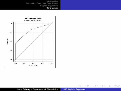
I SAS does the ROC curve for you easily with ODSgraphics and the ”OUTROC=ROC” option after themodel statement.

I Note that in all ROC curve outputs of this type, SAS willtell you the area under the ROC curve. We use thismeasurement to determine how good a fit this model isto the data, by being able to determine how well thefitted model makes predictions. We want an area underthe curve of 0.50 or greater.

I ROC Curves are not limited to logistic regression andaren’t always used in the analysis, but they are an easy todo diagnostic in SAS.


Logistic

Documents

Transcript of Logistic