Logical-Shapelets: An Expressive Primitive for TimeSeries Classification

Abdullah MueenUC Riverside

mueen@cs.ucr.edu

Eamonn KeoghUC Riverside

eamonn@cs.ucr.edu

Neal YoungUC Riverside

neal@cs.ucr.edu

ABSTRACTTime series shapelets are small, local patterns in a time series thatare highly predictive of a class and are thus very useful features forbuilding classifiers and for certain visualization and summarizationtasks. While shapelets were introduced only recently, they havealready seen significant adoption and extension in the community.

Despite their immense potential as a data mining primitive, thereare two important limitations of shapelets. First, their expressive-ness is limited to simple binary presence/absence questions. Sec-ond, even though shapelets are computed offline, the time taken tocompute them is significant.

In this work, we address the latter problem by introducing anovel algorithm that finds shapelets in less time than current meth-ods by an order of magnitude. Our algorithm is based on intelligentcaching and reuse of computations, and the admissible pruning ofthe search space. Because our algorithm is so fast, it creates anopportunity to consider more expressive shapelet queries. In par-ticular, we show for the first time an augmented shapelet repre-sentation that distinguishes the data based on conjunctions or dis-junctions of shapelets. We call our novel representation Logical-Shapelets. We demonstrate the efficiency of our approach on theclassic benchmark datasets used for these problems, and show sev-eral case studies where logical shapelets significantly outperformthe original shapelet representation and other time series classific-ation techniques. We demonstrate the utility of our ideas in do-mains as diverse as gesture recognition, robotics, and biometrics.

Categories and Subject DescriptorsH.2.8 [Database Management]: Database Applications—Data Min-ing

General TermsAlgorithm

KeywordsTime Series, Classification, Information Gain, Logic Expression

Permission to make digital or hard copies of all or part of this work forpersonal or classroom use is granted without fee provided that copies arenot made or distributed for profit or commercial advantage and that copiesbear this notice and the full citation on the first page. To copy otherwise, torepublish, to post on servers or to redistribute to lists, requires prior specificpermission and/or a fee.KDD’11, August 21–24, 2011, San Diego, California, USA.Copyright 2011 ACM 978-1-4503-0813-7/11/08 ...$10.00.

1. INTRODUCTIONTime series shapelets were introduced in 2009 as a primitive for

time series data mining [19]. Shapelets are small sequences thatseparate the time series into two classes by asking the question"Does this unknown object have a subsequence that is within T ofthis shapelet?" Where there are three or more classes, repeated app-lication of shapelets can be used (i.e. a decision tree-like structure)to predict the class label. Figure 1 shows examples of shapeletsfound in a dataset of accelerometer signals [11]. Every time seriesin the dataset corresponds to one of two hand motions performedby an actor tracing a circular or rectangular path through the airwith an input device. The shapelet denoted by P in the figure isthe one that maximally separates the two classes when used witha suitable threshold. In essence, the shapelet P captures the sinu-soidal acceleration pattern of the circular motion along the Z-axis.

X-axis Y-axis Z-axisMotions

(a) (b) (c)

P

α βγ δ

γ

δ

βα

P

Figure 1: (a) Idealized motions performed with a Wii remote.(b) The concatenated accelerometer signals from recordings ofactors performing the motions (c) Examples of Shapelets thatdescribe each of the motions.

Time series shapelets are generating increasing interest amongresearchers [5] [13] [18] for at least two reasons. First, in manycases time series shapelets can learn the inherent structure of thedata in a manner that allows intuitive interpretation. For exam-ple, beyond classifying, say, normal/abnormal heartbeats, shapeletscould tell a cardiologist that the distinguishing feature is at the be-ginning of the dicrotic pulse. Second, shapelets are usually muchshorter than the original time series, and unlike instance based meth-ods that require comparison to the entire dataset, we only need oneshapelet at classification time. Therefore, shapelets create a verycompact representation of the class concept, and this compactnessmeans that the time and space required for classification can be sig-nificantly reduced, often by at least two orders of magnitude. Thisis a particularly desirable property in resource limited systems suchas sensor nodes, cell phones, mobile robots, smart toys, etc.

Despite the above promising features of time series shapelets, thecurrent algorithm [19] for discovering them is still relatively lethar-

gic and, therefore, does not scale up to use on real-world datasets,which are often characterized by being noisy, long, and nonuni-formly sampled. In addition, the current definition of shapelets isnot expressive enough to represent certain concepts that seem quitecommon in the real world (examples appear later in this work). Inparticular, the expressiveness of shapelets is limited to simple bi-nary presence/absence questions. While recursive application ofthese binary questions can form a decision tree-like structure, it isimportant to recognize that the full expressive power of a classic,machine-learning decision tree is not achieved (recall a decisiontree represents the concept space of disjunction of conjunctions).For example, differentiating classes by using only binary questionsis not possible if, the classes differ only in the number of occur-rences of a specific pattern rather than presence/absence of a pat-tern.

In this work, we address the problem of scalability and show howthis allows us to define a more expressive shapelet representation.We introduce two novel techniques to speedup search for shapelets.First, we precompute sufficient statistics [16] to compute the dis-tance (i.e. similarity) between a shapelet and a subsequence of atime series in amortized constant time. In essence, we trade timefor space, finding that a relativity small increase in the space re-quired can help us greatly decrease the time required. Second, weuse a novel admissible pruning technique to skip the costly com-putation of entropy (i.e. the goodness measure) for the vast major-ity of candidate shapelets. We have achieved up to 27× speedupover the current algorithm experimentally. We further show thatwe can combine multiple shapelets in logic expressions such thatcomplex concepts can be described. For example, in the datasetshown in figure 1, there are discontinuities in the rectangular mo-tion. It will not be possible to describe the rectangular class usingone shapelet if there are variable pause times at the corners in diffe-rent instances. In such cases, we can express the rectangular classby the logical shapelet “α and β and γ and δ.” Here, each literalcorresponds to one of the straight line motions as shown in figure1(c). In addition, our algorithm is able to increase the gap/marginbetween classes even if they are already separated. This allows formore robust generalization from the training to test data. We havesuccessfully used our algorithm to find interesting combinations ofshapelets in accelerometer signals, pen-based biometrics, and ac-celerometer signals from a mobile robot.

It is important to note that there is essentially zero-cost for theexpressiveness of logical shapelets. If we apply them to a datasetthat does not need their increased representational power, they sim-ply degenerate to classic shapelets, which are a special case. Thus,our work complements and further enables the growing interest inshapelets as a data mining tool. For example, [18] uses shapeletson streaming data as “early predictors” of a class, [13] uses an ex-tension of shapelets in an application in severe weather prediction,[6] uses shapelets to find representative prototypes in a dataset, and[5] use shapelets to do gesture recognition from accelerometer data.However, none of these works have considered the logical combi-nations of shapelets we consider here or have obtained an signifi-cant speedup over the original algorithm.

2. DEFINITION AND BACKGROUNDIn this section, we define shapelets and the other notations used

in the paper.

Definition 1. A Time Series T is a sequence of real numberst1, t2, . . . , tm. A time series subsequence Si,l = ti, ti+1, . . . , ti+l−1

is a continuous subsequence of T starting at position i and length l.

A time series of length m can have m(m+1)2

subsequences of allpossible lengths from one to m.

If we are given two time series X and Y of same length m, wecan use the euclidean norm of their difference (i.e. X−Y ) as a dis-tance measure. To achieve scale and offset invariance, we must nor-malize the individual time series using z-normalization before theactual distance is computed. This is a critical step; even tiny differ-ences in scale and offset rapidly swamp any similarity in shape [8].In addition, we normalize the distances by dividing with the lengthof the time series. This allows comparability of distances for pairsof time series of various lengths. We call this length-normalization.

The normalized euclidean distance is generally computed by the

formula√

1m

∑mi=1(xi − yi)2. Thus, computing a distance value

requires time linear on the length of the time series. In contrast,we compute the normalized eucledian distance between X and Yusing five numbers derived from X and Y . These numbers are de-noted as sufficient statistics in [16]. The numbers are

∑x,∑y ,∑

x2 ,∑y2 and

∑xy. It may appear that we are doing more work

than necessary; however, as we make clear in section 3.1, comput-ing the distance in this manner enables us to reuse computationsand reduce the amortized time complexity from linear to constant.

The sample mean and standard deviation can be computed fromthese statistics as µx = 1

m

∑x and σ2

x = 1m

∑x2 − µ2

x, re-spectively. The positive correlation and the normalized euclideandistance between X and Y can then be expressed as below [14].

C(x, y) =

∑xy −mµxµy

mσxσy(1)

dist(x, y) =√

2(1− C(x, y)) (2)

Many time series data mining algorithms (1-NN classification, clus-tering, density estimation, etc.) require only the comparison of timeseries that are of equal lengths. In contrast, time series shapeletsrequire us to test if a short time series (the shapelet) is containedwithin a certain threshold somewhere inside a much longer timeseries. To achieve this, the shorter time series is slid against thelonger one to find the best possible alignment between them. Wecall this distance measurement the subsequence distance and defineit as sdist(x, y) =

√2(1− Cs(x, y)) where x and y are the two

time series with lengths m and n, respectively, and for m ≤ n

Cs(x, y) = min0≤l≤n−m

∑mi=1 xiyi+l −mµxµy

mσxσy(3)

In the above definition µy and σy denote the mean and standarddeviation of m consecutive values from y starting at position l+ 1.Note that, sdist is not symmetric.

Assume that we have a dataset D of N time series from C dif-ferent classes. Let us also assume, every class i (i = 1, 2, . . . , C)has ni (

∑i ni = N ) labeled instances in the dataset. An instance

time series in D is also denoted by Di for i = 1, 2, . . . , N .

Definition 2. The entropy of a dataset D is defined as E(D) =

−∑C

i=1niNlog(ni

N).

If the smallest time series in D is of length m, there are at leastN m(m+1)

2subsequences in D that are shorter than every time se-

ries in D. We define a split as a tuple (s, τ) where s is a subse-quence and τ is a distance threshold. A split divides the dataset Dinto two disjoint subsets or partitionsDleft = {x : x ∈ D, sdist(s, x) ≤τ} and Dright = {x : x ∈ D, sdist(s, x) > τ}. We define thecardinality of each partition by N1 = |Dleft| and N2 = |Dright|.

Algorithm 1 Shapelet_Discovery(D)

Require: A dataset D of time seriesEnsure: Return the shapelet1: m← minimum length of a time series in D2: maxGain← 0,maxGap← 03: for j ← 1 to |D| do {every time series in D}4: S ← Dj

5: for l← 1 to m do {every possible length}6: for i← 1 to |S| − l + 1 do {every start position}7: for k ← 1 to |D| do {compute distances of every time

series to the candidate shapelet Si,l}8: Lk ← sdist(Si,l, Dk)9: sort(L)

10: (τ, updated)← bestIG(L,maxGain,maxGap)11: if updated then {gain and/or gap are changed}12: bestS ← Si,l,bestτ ← τ ,bestL← L13: return (bestS, bestτ, bestL,maxGain,maxGap)

Algorithm 2 sdist(x, y)

Require: Two time series x and y. Assume |x| ≤ |y|.Ensure: Return the normalized distance between x and y1: minSum←∞2: x← zNorm(x)3: for j ← 1 to |y| − |x|+ 1 do {every start position on y}4: sum← 05: z ← zNorm(yj,|x|)6: for i← 1 to |x| do {compute the eucledian distance}7: sum← sum+ (zi − xi)28: minSum← min(minSum, sum)

9: return√minSum/|x|

We use two quantities to measure the goodness of a split: informa-tion gain and separation gap.

Definition 3. The information gain of a split is I(s, τ) = E(D)−N1NE(Dleft)− N2

NE(Dright).

Definition 4. The separation gap of a split is G(s, τ) =1

N2

∑x∈Dright

sdist(s, x) − 1N1

∑x∈Dleft

sdist(s, x).

Now we are in position to define time series shapelets.

Definition 5. The shapelet for a dataset D is a tuple of a sub-sequence of an instance within D and a distance threshold (i.e. asplit) that has the maximum information gain while breaking tiesby maximizing the separation gap.

2.1 Brute-force AlgorithmIn order to properly frame our contributions, we begin by ex-

plaining the brute-force algorithm for finding shapelets in a datasetD (algorithm 1). Dataset D contains multiple time series of two ormore classes and possibly of different lengths.

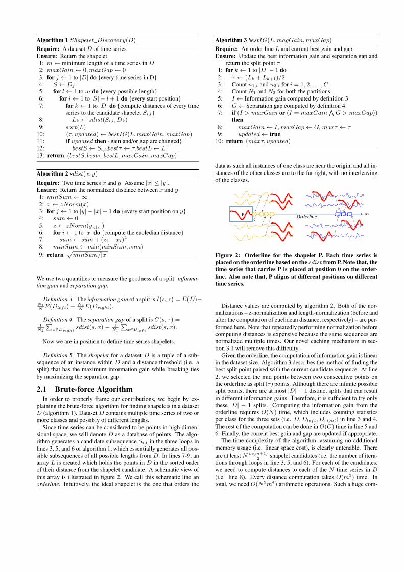
Since time series can be considered to be points in high dimen-sional space, we will denote D as a database of points. The algo-rithm generates a candidate subsequence Si,l in the three loops inlines 3, 5, and 6 of algorithm 1, which essentially generates all pos-sible subsequences of all possible lengths from D. In lines 7-9, anarray L is created which holds the points in D in the sorted orderof their distance from the shapelet candidate. A schematic view ofthis array is illustrated in figure 2. We call this schematic line anorderline. Intuitively, the ideal shapelet is the one that orders the

Algorithm 3 bestIG(L,magGain,maxGap)

Require: An order line L and current best gain and gap.Ensure: Update the best information gain and separation gap and

return the split point τ1: for k ← 1 to |D| − 1 do2: τ ← (Lk + Lk+1)/23: Count n1,i and n2,i for i = 1, 2, . . . , C.4: Count N1 and N2 for both the partitions.5: I ← Information gain computed by definition 36: G← Separation gap computed by definition 47: if (I > maxGain or (I = maxGain

∧G > maxGap))

then8: maxGain← I , maxGap← G, maxτ ← τ9: updated← true

10: return (maxτ, updated)

data as such all instances of one class are near the origin, and all in-stances of the other classes are to the far right, with no interleavingof the classes.

P Orderline0

Figure 2: Orderline for the shapelet P. Each time series isplaced on the orderline based on the sdist from P. Note that, thetime series that carries P is placed at position 0 on the order-line. Also note that, P aligns at different positions on differenttime series.

Distance values are computed by algorithm 2. Both of the nor-malizations – z-normalization and length-normalization (before andafter the computation of euclidean distance, respectively) – are per-formed here. Note that repeatedly performing normalization beforecomputing distances is expensive because the same sequences arenormalized multiple times. Our novel caching mechanism in sec-tion 3.1 will remove this difficulty.

Given the orderline, the computation of information gain is linearin the dataset size. Algorithm 3 describes the method of finding thebest split point paired with the current candidate sequence. At line2, we selected the mid points between two consecutive points onthe orderline as split (τ ) points. Although there are infinite possiblesplit points, there are at most |D| − 1 distinct splits that can resultin different information gains. Therefore, it is sufficient to try onlythese |D| − 1 splits. Computing the information gain from theorderline requires O(N) time, which includes counting statisticsper class for the three sets (i.e. D,Dleft, Dright) in line 3 and 4.The rest of the computation can be done inO(C) time in line 5 and6. Finally, the current best gain and gap are updated if appropriate.

The time complexity of the algorithm, assuming no additionalmemory usage (i.e. linear space cost), is clearly untenable. Thereare at leastN m(m+1)

2shapelet candidates (i.e. the number of itera-

tions through loops in line 3, 5, and 6). For each of the candidates,we need to compute distances to each of the N time series in D(i.e. line 8). Every distance computation takes O(m2) time. Intotal, we need O(N2m4) arithmetic operations. Such a huge com-

putational cost makes the brute-force algorithm infeasible for realapplications. Since N is usually small as being the size of a la-beled dataset, and m is large to make the search for local featuresmeaningful, we focus on reducing factors of m from the cost.

3. SPEEDUP TECHNIQUESThe original shapelet work introduced by Ye, et al. [19] showed

an admissible technique for abandoning some unfruitful entropycomputations early. However, this does not improve the worst casecomplexity. In this work, we reduce the worst case complexityby caching distance computations for future use. In addition, wedescribe a very efficient pruning strategy resulting in an order ofmagnitude speedup over the method of Ye et al..

3.1 Efficient Distance ComputationIn algorithm 1, any subsequence ofDj with any length and start-

ing at any position is a potential shapelet candidate. Such a candi-date needs to be compared against every subsequence of Dk withthe same length, starting at any position. The visual intuition ofthe situation is illustrated by figure 3. For any two instances Dj

and Dk in D, we need to consider all possible parallelograms likethe ones shown in the figure. For each parallelogram, we need toscan the subsequences to sum up the squared errors while comput-ing the distance. Clearly there is a huge redundancy of calculationsbetween successive and overlapping parallelograms.

1 lv

1 lu

u

v(a) (b)

Dj

Dk

l

u

v

Figure 3: (a) Illustration of a distance computation requiredbetween a pair of subsequences starting at positions u and v,respectively, and of length l. Dashed lines show other possibledistance computations. (b) The matrix M for computing thesum of products of the subsequences in (a).

Euclidean distance computation for subsequences can be madefaster by reusing overlapping computation. However, reusing com-putations of z-normalized distances for overlapping subsequencesneeds at least quadratic space and, therefore, is not tenable formost applications. When we need all possible pairwise distancesamong the subsequences, as we do in finding shapelets, spendingthe quadratic space saves a whole order of magnitude of computa-tion time.

For every pair of points (Dj , Dk) we compute five arrays. Werepresent these arrays as Statsx,y in the algorithms. Two of thearrays (i.e. Sx and Sy) store the cumulative sum of the individualtime series x and y. Another two (i.e. Sx2 and Sy2 ) store thecumulative sum of squared values. The final one (i.e. M) is a 2Darray that stores the sum of products for different subsequences ofx and y. The arrays are defined mathematically below. All of thearrays have left margin of zero values indexed by 0. More precisely,Sx[0], Sy[0], Sx2 [0], Sy2 [0], M[0, 0], M[u, 0] for u = 1, 2, . . . , |x|,and M[0, v] for v = 1, 2, . . . , |y| are all zeros.

Sx[u] =∑u

i=0 xi , Sy[v] =∑v

i=0 yi,Sx2 [u] =

∑ui=0 x

2i , Sy2 [v] =

∑vi=0 y

2i

M[u, v] =

{ ∑vi=0 xi+tyi if u > v,∑ui=0 xiyi+t if u ≤ v

Algorithm 4 sdist_new(u, l, Statsx,y)

Require: start position u and length l and the sufficient statisticsfor x and y.

Ensure: Return the subsequence distance between xu,l and y1: minSum←∞2: {M, Sx, Sy, Sx2 , Sy2} ← Statsx,y3: for v ← 1 to |y| − |x|+ 1 do4: d← distance computed by (1) and (2) in constant time5: if d < minSum then6: minSum← d7: return

√minSum

where t = abs(u− v).Given that we have computed these arrays, the mean, variance,

and the sum of products for any pair of subsequences of the samelength can be computed as below.

µx = Sx[u+l−1]−Sx[u−1]l

, µy =Sy [v+l−1]−Sy [v−1]

l

σx =Sx2 [u+l−1]−S

x2 [u−1]

l−µ2

x, σy =Sy2 [v+l−1]−S

y2 [v−1]

l−µ2

y∑l−1i=0 xu+iyv+i = M[u+ l − 1, v + l − 1]−M[u− 1, v − 1].

This in turn means that the normalized euclidean distance (theinformation we actually want) between any two subsequences xu,land yv,l of any length l can now be computed using equations 1and 2 in constant time. The algorithm 4 describes the steps. Thealgorithm takes as input the starting position u and the length l ofthe subsequence of x. It also takes the precomputed Statsx,y car-rying the sufficient statistics. The algorithm iterates for all possiblestart positions v of y and returns the minimum distance. Thus wecan see that the procedure sdist_new saves at least anO(m) innerloop computation from procedure sditst.

3.2 Candidate PruningThe constant time approach for distance computation introduced

in the previous section helps reduce the total cost of shapelet dis-covery by a factor of m. Our next goal is to reduce the numberof iterations that occur in the for loop at line 6 in the algorithm 1.The core idea behind our attack on this problem is the followingobservation: If we know (s, τ) is a poor shapelet (i.e. it has lowinformation gain) then any similar subsequence to s must also re-sult in a low information gain and, therefore, a costly evaluation(computing all the distances) can be safely skipped. Assume wehave observed a good best-so-far shapelet at some point in the al-gorithm. Let us denote this shapelet (Sp, τp) and its informationgain Ip. Imagine we now test (Si,l, τ), and it has very poor in-formation gain Ii,l < Ip. Let us consider the next subsequenceSi+1,l. Here is our fundamental question. Is it possible to use therelationship (the Euclidean distance) between Si,l and Si+1,l, toprune Si+1,l?

To develop our intuition, let us first imagine a pathological case.Suppose that dist(Si,l, Si+1,l) = 0; in other words, Si+1,l is theexact same shape as Si,l. In that case we can obviously pruneSi+1,l, since its information gain must also be Ii,l. Suppose, how-ever, in the more realistic case, that Si,l and Si+1,l are similar, butnot identical. We may still be able to prune Si+1,l. The trick is toask, “how good could Si+1,l be?” , or a little more formally, “Whatis an upper bound on the information gain of Si+1,l”. It turns outthat it is simple to calculate this bound!

Let the distance between Si,l and Si+1,l be R. By triangular in-equality, sdist(Si+1,l, Dk) can be as low as sdist(Si,l, Dk) − Rand as high as sdist(Si,l, Dk) + R regardless of the alignment of

Si+1,l onDk. Thus, every point on the orderline of Si,l has a “mo-bility” in the range [−R,R] from its current position. Given thismobility, our goal is to find the best configuration of the points thatgives maximum information gain when split into two partitions.The points that lie outside [τ −R, τ +R] can have no effect on theinformation gain for candidate (Si+1,l, τ). For the points inside[τ −R, τ +R] we can shift them optimistically in either directionto increase the information gain.

Every class c ∈ C has nc instances in the database which are di-vided into two partitions by a split. Let nc,1 and nc,2 be the numberof instances of class c in partition Dleft and Dright, respectively.A class is weighted to the left (or simply called left-major/right-minor) if nc,1

N1>

nc,2

N2. Similarly, a class is called right-major/left-

minor if nc,1

N1≤ nc,2

N2. The following lemma describes the optimal

choice for a single point. We relegate the proof to Appendix toenhance the flow of the paper.

THEOREM 1. Shifting a point from its minor partition to its ma-jor partition always increases information gain.

If we shift a point from the minor partition to the major partition,the major/minor partitions of the class remain the same as beforeshifting, simply because, if nc,1

N1>

nc,2

N2then nc,1+1

N1+1>

nc,2−1

N2−1.

Therefore, shifting all the minor points of a class to its major par-tition increases the information gain monotonically, and thus, thiscan be treated as an atomic operation. We denote such a sequenceof shifts as a “transfer”. Transferring a class may change the major-minor partitions of other classes and, consequently, the transfer di-rection for that class. Therefore, if we transfer every class basedon the major-minor partitions in the initial orderline, it does notnecessarily guarantee the maximum information gain.

In the case of two-class datasets, there is always one left-majorand one-right major class. Therefore, shifting all of the points in[τ − R, τ + R] to their major partition will not change the major-minor partitions of either of the classes; thus, this guarantees theoptimization (i.e. the upper bound) even if the initial transfer direc-tions are used.

For a case of more than two-classes, almost all of the time initialmajor-minor partitions hold after all of the transfers are done. Un-fortunately, it is possible to construct counter examples, even if werarely confront them on real data. To obtain the optimal bound weneed to try all possible transfer directions for all of the classes re-sulting in 2C trials. Fortunately, many classification problems dealwith a small number of classes. For example, 60% of the UCR timeseries datasets have four or less classes. Given this fact, having the2C constant in the complexity expression will not be an issue formany problems.

Algorithm 5 describes the computation of the upper bound. Thealgorithm loops through all distinct split positions (line 2-3). Forevery split position, the algorithm transfers all of the classes to theirmajor partition based on the initial orderline (line 5-6) and com-putes the information gain to find the upper bound. Note that line 4is “commented out” in the algorithm which is a for loop that checksall of the 2C combinations of transfer directions. For exact bound inthe case of many-class datasets, this line should be uncommented.

To summarize, for the two-class case we have an exact and ad-missible pruning technique. In the multi-class case we have a pow-erful heuristic that empirically gives answers that are essentiallyindistinguishable from the optimal answer.

3.3 The Fast Shapelet Discovery AlgorithmWith the speedup techniques described in the previous section,

we are now ready to plug them into algorithm 1 and build a fasterversion as shown in algorithm 6.

0 5 10 15-2

-1

0

1

2R = dist(S1,S2)

S1

τR R

S2

τ

Left-major ClassRight-major Class

Information Gain (S1,τ) =

5

2log

10

2

5

3log

10

3

2

1log

Upper Bound (S2,τ) =

S2

τ 5

4log

10

4

5

1log

10

1

2

1log

(a) (b)

(d)(c)

After transfers

Before transfers

0

0

0

Figure 4: (a) A sequence S1 and its orderline. (b) Distancebetween the sequences S1 and S2 is R. (c) The points on theorderline within [τ −R, τ +R] are transferred to their major-ity partition. (d) The computation of the information gain for(S1, τ) and upper bound for (S2, τ).

Algorithm 5 upperIG(L,R)

Require: An order line L and the candidate distance R.Ensure: Return an upper bound of information gain.1: maxI ← 02: for k ← 1 to |D| − 1 except j do3: τ ← (Lk + Lk+1)/24: //for all 2C combinations of transfer directions do5: for all points p ∈ [τ −R, τ +R]6: move p to its majority end.7: Count n1,i and n2,i for i = 1, 2, . . . , C.8: Count N1 and N2 for both the partitions.9: I ← information gain computed by definition 3

10: maxI ← max(maxI, I)11: return maxI

In lines 5-7, the sufficient statistics are computed for the currenttime series Dj paired with every other time series Dk.

The algorithm maintains a set of orderlines in the history H . Forevery candidate Si,l, before committing to the expensive computa-tion of the orderline, the algorithm quickly computes upper boundsusing the orderlines in the history (line 14). If any of the upperbounds is smaller than the maximum gain achieved so far we cansafely abandon the candidate (line 15).

Since the upper bound computation is based upon the triangu-lar inequality, we are only allowed to use the previous orderlinescomputed for sequences of the same length as the current candi-date 1. Therefore, once the search moves on to the next length thealgorithm clears the history H and starts building it up for the newlength (line 9).

The size of the history H is a user-defined value and the algo-rithm is insensitive to this value once it is set to at least five. Toprevent our history cache in line 22 growing without bound, weneed to have a replacement policy. The oldest-first (LIFO) policyis the most suitable for this algorithm. This is because the recentsubsequences tend to be correlated with the current candidate and,therefore, have small distances from the candidate. Note that, wedo not add all orderlines to the history. We only add the orderlinesthat have less information gain (i.e. orderlines for poor shapeletcandidate) than the current maxGain. Because only poor candi-

1The reader may wonder why we cannot create a bound betweena sequence and a shorter sequence that is its prefix. Such boundscannot be created because we are normalizing all sequences, andafter normalizing the distances may increase or decrease.

Algorithm 6 Fast_Shapelet_Discovery(D)

Require: A dataset D of time seriesEnsure: Return the shapelet1: m← minimum length of a time series in D2: maxGain← 0,maxGap← 03: for j ← 1 to |D| do {every time series in D}4: S ← jth time series of D5: for k ← 1 to |D| do {compute statistics for S and Dk}6: x← S, y ← Dk

7: Statsx,y ← {M, Sx, Sy, Sx2 , Sy2}8: for l← 1 to m do {every possible length}9: clear H

10: for i← 1 to |S| do {every start position}11: for w ← 1 to |H| do {every candidate in H}12: (L′, S′)← H[w]13: R← sdist(Si,l, S

′)14: if upperIG(L′, R) < maxGain then {prune this

candidate}15: continue with next i16: for k ← 1 to |D| do {since not pruned; compute dis-

tances of every time series to the candidate Si,l}17: Lk ← sdist_new(i, l, Statsx,y)18: sort(L)19: (τ, updated)← bestIG(L,maxGain,maxGap)20: if updated then {gain and/or gap are changed}21: bestS ← Si,l,bestτ ← τ ,bestL← L22: add (L, Si,l) to H if maxGain is not changed23: return (bestS, bestτ, bestL,maxGain,maxGap)

dates have the power of pruning similar candidates by predictingtheir low information gain.

4. LOGICAL SHAPELETA shapelet is a tuple consisting of a subsequence and a split point

(threshold) that attempts to separate the classes in exactly two dif-ferent groups. However, it is easy to imagine situations where itmay not be sufficient to use only one shapelet to achieve separationof classes, but a combination of shapelets. To demonstrate this, weshow a simple example. In Figure 5(a), we have a two-class prob-lem where each class has two time series. The square class con-tains two sinusoidal patterns with both positive and negative peaks,while the circle class has only one positive or one negative peak.If we attempt to use the classic shapelet definition to separate theseclasses, we find there is no way to do so. Classic shapelets sim-ply do not have the expressiveness to represent this concept. Thereason is that every single distinct pattern appears in both of theclasses, or in only one of the time series of one of the classes. Forexample, in 5(b) three different unary shapelets and their orderlinesare illustrated, and none of them achieved a separation between theclasses.

To overcome this problem, we propose using multiple shapeletswhich allow distinctions based on logical combinations of the shapelets.For example, if we use the first two shapelets in figure 5(b) thenwe can say that (S1, τ1) and (S2, τ2) separate the classes best.From now on, we use standard logic symbols

∧and

∨for and

and or operations. For a new instance x, if sdist(S1, x) < τ1∧sdist(S2, x) < τ2 is true, then we can classify x as a mem-

ber of the square class, or otherwise the circle class. When us-ing multiple shapelets in such a way, chaining of logical combi-nations among the shapelets is possible; for example, (S1, τ1)

∧(S2, τ2)

∨(S3, τ3). However, for the sake of simplicity and to

guard against over fitting with too complex a model [4], we onlyconsider two cases, only

∧, and only

∨combinations. We further

guard against overfitting with too flexible a model by allowing onlyjust a single threshold for both shapelets.

We have already seen how to create an orderline for classic shapelets,how do we define an orderline for conjunctive or disjunctive shapelets?To combine the orderlines for such cases, we adopt a very simpleapproach. For

∧operation, the maximum of the distances from

the literal shapelets is considered as the distance on the new order-line, and for

∨the minimum is considered. Apart from these minor

changes, the computation of the entropy and information gain areunchanged.

For example, in figure 5(d) the combined orderline for (S1

∧S2, τ) is shown. The two classes are now separable because boththe shapelets occur together in the square class and do not bothoccur together in individual instances of the circle class.

Given these minor changes to allow logical shapelets, we canstill avail ourselves of the speedup techniques proposed in section3. The original shapelet algorithm just needs to be modified to runmultiple times, and some minor additional bookkeeping must bedone. When the first shapelet is found by the algorithm 6, we nowtest to see if there is any class whose instances are in both the parti-tions of the optimal split. We call such a class “broken” (We couldsay “non-linearly separable,” however, our situation has a slightlydifferent interpretation). If there is a broken class, we continue tosearch for a new shapelet on the same dataset that can merge theparts of the broken class. However, this time we must make surethat new shapelet does not have a match with a subsequence in Dk

that overlaps with the matching subsequence of an already discov-ered shapelet. After finding the new shapelet, we combine the or-derlines and the threshold based on the appropriate logic operation.Finally, we are in position to measure the information gain to see ifit is better than our best-so-far. If the gain improves, we test for abroken class again and continue as before. Once there is no brokenclass or the gain does not increase, we recursively find shapelet(s)in the left and right partitions.

The above approach is susceptible to overfitting. It can degen-erate into (S1, τ1)

∨(S2, τ2)

∨. . .∨

(Sni , τn) where ni is thenumber of instances in the class i and each Sj for j = 1, 2, . . . , ni

is a subsequence of different instances of class i in the dataset D.In this case, all of the instances of class i would be in the left sidewith zero distances. To avoid overfitting, we can have a hard boundon the number of literals in the logic expression. In this work, thebound is hard coded to four, however, for a very large dataset wecould slowly increase this number, if we carefully check to guardagainst overfitting. Note that the situation here is almost perfectlyanalogous to the problem of overfitting in decision trees, and weexpect that similar solutions could work here.

5. EVALUATIONWe begin by noting that we have taken extraordinary lengths

to make all our experiments reproducible. As such, all code anddata are available at [2], and will be maintained there in perpetuity.Moreover, while our proposed algorithm is not sensitive to the fewparameters required as inputs, we explicitly state all parameters forevery dataset at [2].

We wish to demonstrate two major points with our experiments.First, our novel speedup techniques can be used to find both classicand logical shapelets significantly faster. Second, there exist real-world problems for which logical shapelets are significantly moreaccurate than classic shapelets or other state-of-the-art techniques(see section 6).

To demonstrate the speedup, we have taken 24 datasets from the

S3

No Separation

Good Separation

(b)

(c)S1 and S2(a)

0 100 200 300 400 500 600 700 800 900 1000-1

-0.5

0

0

0.5

1

-1

0

1

-1

0

1

0 100 200 300 400 500 600 700 800 900 1000

1

2

3

4

4

3

1

S1

S2

τ

A dataset

0

0

0

0

Figure 5: (a) Two classes of synthetic time series. (b) Examplesof single shapelets that cannot separate the classes. Any othersingle shapelet would fail similarly. (c) Two shapelets connectedby an and operation can separate the classes.

UCR time series archive [9]. For brevity the names and propertiesof these datasets and tables of time taken for running the shapeletalgorithms on these datasets can be found at [2]. Here we contentourselves with a visual summary. In figure 6(left), we show thespeedups over the original algorithm. Our algorithm obtained somespeedup for all of the datasets with a maximum of 27.2.

The two speedup methods described in section 3 are not inde-pendent of each other. Therefore, we also measure the individualspeedups for each of the techniques while deactivating the other.The individual speedup factors for both the techniques are plot-ted in figure 6(right). There is no speedup for two of the datasets(shown by stars) when only the candidate pruning method is active.The reason is that the amount of pruning achieved for these datasetscannot surpass the overhead costs of computing the upper boundsfor every candidate. However, when the technique of efficient dis-tance computation is active, speedups are achieved for all of thedatasets including these two.

101

102

103

104

105

100

101 102 103 104 105

106

106100

Ru

nn

ing

tim

e fo

r O

rigi

nal

Met

ho

d (

sec)

Running time for theOur Method (sec)

In this region our method is

better

In this region original method

is better0 2 4 6 8 10 12 14 16 18

0

1

2

3

4

5

6

Spee

du

p f

or

Can

did

ate

Pru

nin

g

Speedup for Efficient Distance Computation

Figure 6: (left) Comparison of running times between ourmethod and the original shapelet algorithm. Note the log scaleon both axes. (right) The individual speedup factors for bothof our proposed techniques: Candidate Pruning and EfficientDistance Computation.

It is critical to note that our improvements in speed are not dueto trivial differences in hardware or to simple implementation op-timizations, but reflect the utility of the two original techniques in-troduced in section 3. In particular, all experiments were done onexactly the same environment and on the same input data files. Thecode for the original shapelet discovery algorithm was graciouslydonated by Dr. Ye who also confirmed that we are using her codein the best possible manner. Since our technique reduced the worstcase complexity by a factor of m and has an admissible pruning

technique which is not present in the original code, we can be surethat the speedup is valid.

As described in section 3.2, our linear time upper bound is notadmissible for the many-class cases. Among the 24 datasets weused for scalability experiments, 13 datasets have more than twoclasses. For these 13 datasets, the average rate of computing falseupper bound is just 1.56% with a standard deviation of 2.86%. Inreality, the impact of false bounds on the final result is inconsequen-tial because of the massive search space for shapelet. Our algorithmrarely misses the optimal information gain in that space and has notmissed in any of the above 13 many-class datasets.

6. CASE STUDIESIn this section we show three case studies in three different do-

mains. In all the case studies we demonstrate that logical combina-tions of shapelets can describe the difference between the classesvery robustly. We compare our algorithm to the 1-NN classifierusing Dynamic Time Warping (DTW) because a recent extensivecomparison of dozens of time series classification algorithms, ondozens of datasets, strongly suggests that 1-NN DTW is exception-ally difficult to beat [3]. Note that the 1-NN classifier using DTWis less amenable for realtime classification of time series since itrequires an O(m2) distance measure to be computed for every in-stance in the dataset. In contrast, classification with shapelets re-quires just a singleO(n(m−n)) calculation (n is the length of theshapelet). Thus, classification with time series shapelets is typicallythousands of times faster than 1-NN DTW. We do not experimen-tally show this here, since it was amply demonstrated in the originalshapelet paper [19].

6.1 Cricket: Automatic ScorerIn the game of cricket (a very popular game in British Common-

wealth countries), an umpire signals different events in the game toa distant scorer/book-keeper. Typically, the signals involve particu-lar motions of the hands. For example, the umpire stretches up boththe hands above the head to signal a score of “six.” A complete listof signals can be found in [1]. Researchers have recently begun toattempt to classify these signals automatically to ease/remove thetask of a scorer [10].

In [10], a dataset was collected in which two accelerometers havebeen placed on both wrists of four different umpires. The umpiresperformed twelve different signals used in the game of cricket atleast ten times. For simplicity of presentation, we select only twoclasses from the dataset that has a unique possibility of confusion.The two classes are “No Ball” and “Wide Ball.” To signal “NoBall,” the umpire must raise one of his hands to the shoulder-heightand keep his hand horizontal until the scorer confirms the record.To signal “Wide Ball,” the umpire stretches both of the hands hori-zontally at shoulder-height (see figure 7).

Each accelerometer has three synchronous and independent mea-surements for three axes (X,Y, and Z). For every signal performed,the six channels are concatenated to form one time series. We ap-pend low variance white noise to each example in the dataset tomake them of length 308. The training set has nine examples asshown in figure 7. The test set has 98 examples. Note that theexamples for “No Ball” are only right hand signals. This is truefor the test set also. To cover the left handed case and also to in-clude examples of different lengths, we have generated another testset using the accelerometer on a standard smart phone. This testset contains 64 examples of length 600. Each class has an equalnumber of examples in both of the training sets.

On this dataset, we performed 1-NN classification using Eu-clidean distance and Dynamic Time Warping (DTW) as distance

Algorithms Original Test set New Test set1-NN Euclidean distance 94.89% 56.25%

1-NN Dynamic Time Warping 98.98% 87.50%1-NN DTW-Sakoe-Chiba 94.89% 75.00%

Shapelet 44.89% 48.43%Logical Shapelet 95.91% 89.06%

Table 1: The accuracies of different algorithms on the two testsets.

measures. We also considered DTW with the Sakoe-Chiba band[15], as it has been shown to outperform classic DTW on manydatasets [7]. The results are shown in table 1. It is interesting toconsider why Logical Shapelets generalize the new data the best.We conjecture that it is the ability of Logical Shapelets to extractjust the meaningful part of the signal. In contrast, DTW and Eu-clidean distance must account for the entire time series, includingsections that may be unique to individual umpires idiosyncratic mo-tion, but not predictive of the concept.

The Computationally expensive 1-NN DTW performs well inboth of the cases, but not suitable for real-time applications. Theoriginal shapelet algorithm fails to capture the fact that the inherentdifference between the classes is in the number of occurrences ofthe shapelet. Our logical shapelet algorithm captures the sharp risesin the Z-axes for “Wide Ball” from the original training set. Nosuch “No Ball" signal can have two such rises in the Z-axes, andtherefore, classification accuracy does not decrease significantly forthe new test set.

50 100 150 200 250 300

-0.2

-0.1

0

0.1and Shapelet Shapelet

No

Bal

lW

ide

Bal

l

-0.2

-0.1

0

0.1

50 100 150 200 250 300

-0.2

-0.1

0

0.1

Right Hand Left HandZ X Y Z X Y

50 100 150 200 250 300

-0.2

-0.1

0

0.1

(a) Signals

(b) (c)

Figure 7: (a)The training set of the cricket dataset by concate-nating signals from every axis of the accelerometer. (b) Thetwo signs an umpire performs to declare two types of illegal de-livery. (c) Shapelets found by our algorithm and the originalalgorithm.

6.2 Sony AIBO Robot: Surface DetectionThe SONY AIBO Robot is a small, dog-shaped, quadruped robot

that comes equipped with multiple sensors, including a tri-axial ac-celerometer. We consider a dataset created by [17] where mea-surements of the accelerometer are collected. In the experimentalsetting, the robot walked on two different surfaces: carpet and ce-ment. For simplicity we consider only the X-axis readings. A snapshot of the data is shown in figure 8(a). Each time series representsone walk cycle. Cemented floors are hard compared to carpets and,therefore, offer more reactive force than carpets. As such, there areclear and sharp changes in the acceleration on the cemented floor.

Algorithms Surface Detection Passgraphs1-NN Euclidean distance 69.55% 63.36%

1-NN Dynamic Time Warping 72.55% 71.76%1-NN DTW-Sakoe-Chiba 69.55% 74.05%

Shapelet 93.34% 60.31%Logical Shapelet 96.34% 70.23%

Table 2: The accuracies of different algorithms on the pass-graph trajectories and accelerometer signals from SONYAIBO robot.

In addition, there is a much larger variability when the robot walkson cement.

The test set has 20 instances of walk cycles on the two types offloors. The training set has 601 instances. A walk cycle is of length70 at 125 hertz. We have experimented on this dataset and found apair of shapelets shown in figure 8(b). The shapelets are connectedby∧

and come from the two different shifts-of-weight in the walkcycle on the carpet floor. The pair of shapelets has a significantlyhigher classification accuracy compared to classic nearest neighboralgorithms (see table 2).

0 10 20 30 40 50 60 70-4

-2

0

2

4

0 10 20 30 40 50 60 70-4

-2

0

2

and Shapelet0 10 20 30 40 50 60 70

-4

-2

0

2

(a) (b)

(c)

Walking on Carpet (Smooth)

Walking on Cement (Hard)

Walking on Carpet

Steps

Figure 8: (a) Two classes of time series from the SONY AIBOaccelerometer. (b) The and-shapelets from the walk cycle oncarpet. (c) The Sony AIBO Robot.

6.3 Passgraphs: Preventing Shoulder-SurfersPassgraphs are a recently proposed biometric system used to au-

thenticate a person and allow her access to some resource. A gridof dots is presented to the user and she is tasked to connect someof the dots in the grid in some specific order as a password. Incontrast to text-based passwords where the user can shield the theentered text (at an ATM for example), Passgraphs are vulnerable to“shoulder-surfing” as it is easy for a miscreant to see and memorizethe connection sequence over the shoulder of the user. To preventthe shoulder-surfing attack, [12] has proposed methods involvingpen-pressure. There are also methods based on other pen proper-ties such as friction, acceleration, etc.

In this case study, we use the data from [12] to see if logicalshapelets can classify between the same pen sequences performedby different users. We selected x-axis trajectories of two differentusers drawing the same passgraph. The logical shapelet shown infigure 9 consists of tiny fragments of the three turns (peaks in thetime series) in the passgraph connected by

∨operations. These

shapelets have better accuracies than 1-NN classifier and are promis-ing enough to use in a real authentication system. This is becausethe shapelets can be learned at training time when the user sets thepassword, and it is not possible for the shoulder surfer to mimicthe idiosyncratic pen path of the real user when attempting to im-personate her. Note that,

∧operations in this case would have

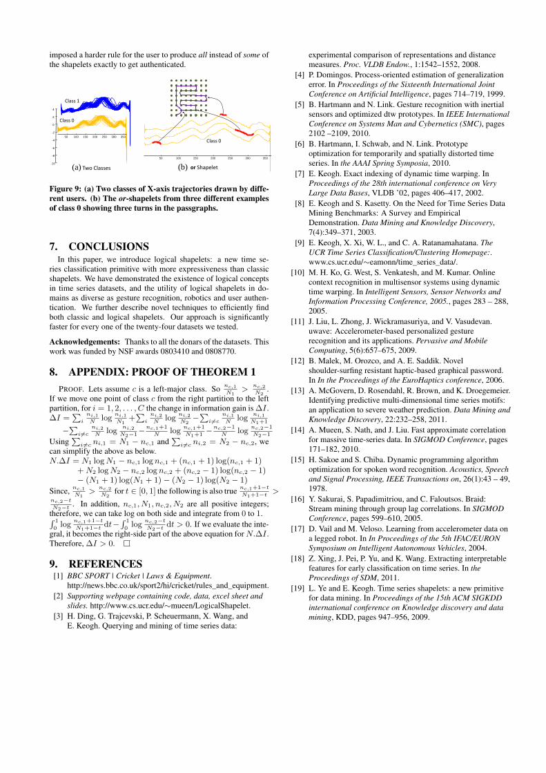
imposed a harder rule for the user to produce all instead of some ofthe shapelets exactly to get authenticated.

-10

-8

-6

-4

-2

0

2

4

50 100 150 200 250 300 350

Class 0

Class 1

50 100 150 200 250 300 350

or Shapelet

Class 0

(a) (b)Two Classes

Figure 9: (a) Two classes of X-axis trajectories drawn by diffe-rent users. (b) The or-shapelets from three different examplesof class 0 showing three turns in the passgraphs.

7. CONCLUSIONSIn this paper, we introduce logical shapelets: a new time se-

ries classification primitive with more expressiveness than classicshapelets. We have demonstrated the existence of logical conceptsin time series datasets, and the utility of logical shapelets in do-mains as diverse as gesture recognition, robotics and user authen-tication. We further describe novel techniques to efficiently findboth classic and logical shapelets. Our approach is significantlyfaster for every one of the twenty-four datasets we tested.

Acknowledgements: Thanks to all the donars of the datasets. Thiswork was funded by NSF awards 0803410 and 0808770.

8. APPENDIX: PROOF OF THEOREM 1PROOF. Lets assume c is a left-major class. So nc,1

N1>

nc,2

N2.

If we move one point of class c from the right partition to the leftpartition, for i = 1, 2, . . . , C the change in information gain is ∆I .∆I =

∑i

ni,1

Nlog

ni,1

N1+∑

i

ni,2

Nlog

ni,2

N2−∑

i 6=c

ni,1

Nlog

ni,1

N1+1

−∑

i 6=c

ni,2

Nlog

ni,2

N2−1−nc,1+1

Nlog

nc,1+1

N1+1−nc,2−1

Nlog

nc,2−1

N2−1

Using∑

i6=c ni,1 = N1 − nc,1 and∑

i 6=c ni,2 = N2 − nc,2, wecan simplify the above as below.N.∆I = N1 logN1 − nc,1 lognc,1 + (nc,1 + 1) log(nc,1 + 1)

+N2 logN2 − nc,2 lognc,2 + (nc,2 − 1) log(nc,2 − 1)− (N1 + 1) log(N1 + 1)− (N2 − 1) log(N2 − 1)

Since, nc,1

N1>

nc,2

N2for t ∈ [0, 1] the following is also true nc,1+1−t

N1+1−t>

nc,2−t

N2−t. In addition, nc,1, N1, nc,2, N2 are all positive integers;

therefore, we can take log on both side and integrate from 0 to 1.∫ 1

0log

nc,1+1−t

N1+1−tdt−

∫ 1

0log

nc,2−t

N2−tdt > 0. If we evaluate the inte-

gral, it becomes the right-side part of the above equation forN.∆I .Therefore, ∆I > 0.

9. REFERENCES[1] BBC SPORT | Cricket | Laws & Equipment.

http://news.bbc.co.uk/sport2/hi/cricket/rules_and_equipment.[2] Supporting webpage containing code, data, excel sheet and

slides. http://www.cs.ucr.edu/∼mueen/LogicalShapelet.[3] H. Ding, G. Trajcevski, P. Scheuermann, X. Wang, and

E. Keogh. Querying and mining of time series data:

experimental comparison of representations and distancemeasures. Proc. VLDB Endow., 1:1542–1552, 2008.

[4] P. Domingos. Process-oriented estimation of generalizationerror. In Proceedings of the Sixteenth International JointConference on Artificial Intelligence, pages 714–719, 1999.

[5] B. Hartmann and N. Link. Gesture recognition with inertialsensors and optimized dtw prototypes. In IEEE InternationalConference on Systems Man and Cybernetics (SMC), pages2102 –2109, 2010.

[6] B. Hartmann, I. Schwab, and N. Link. Prototypeoptimization for temporarily and spatially distorted timeseries. In the AAAI Spring Symposia, 2010.

[7] E. Keogh. Exact indexing of dynamic time warping. InProceedings of the 28th international conference on VeryLarge Data Bases, VLDB ’02, pages 406–417, 2002.

[8] E. Keogh and S. Kasetty. On the Need for Time Series DataMining Benchmarks: A Survey and EmpiricalDemonstration. Data Mining and Knowledge Discovery,7(4):349–371, 2003.

[9] E. Keogh, X. Xi, W. L., and C. A. Ratanamahatana. TheUCR Time Series Classification/Clustering Homepage:.www.cs.ucr.edu/∼eamonn/time_series_data/.

[10] M. H. Ko, G. West, S. Venkatesh, and M. Kumar. Onlinecontext recognition in multisensor systems using dynamictime warping. In Intelligent Sensors, Sensor Networks andInformation Processing Conference, 2005., pages 283 – 288,2005.

[11] J. Liu, L. Zhong, J. Wickramasuriya, and V. Vasudevan.uwave: Accelerometer-based personalized gesturerecognition and its applications. Pervasive and MobileComputing, 5(6):657–675, 2009.

[12] B. Malek, M. Orozco, and A. E. Saddik. Novelshoulder-surfing resistant haptic-based graphical password.In In the Proceedings of the EuroHaptics conference, 2006.

[13] A. McGovern, D. Rosendahl, R. Brown, and K. Droegemeier.Identifying predictive multi-dimensional time series motifs:an application to severe weather prediction. Data Mining andKnowledge Discovery, 22:232–258, 2011.

[14] A. Mueen, S. Nath, and J. Liu. Fast approximate correlationfor massive time-series data. In SIGMOD Conference, pages171–182, 2010.

[15] H. Sakoe and S. Chiba. Dynamic programming algorithmoptimization for spoken word recognition. Acoustics, Speechand Signal Processing, IEEE Transactions on, 26(1):43 – 49,1978.

[16] Y. Sakurai, S. Papadimitriou, and C. Faloutsos. Braid:Stream mining through group lag correlations. In SIGMODConference, pages 599–610, 2005.

[17] D. Vail and M. Veloso. Learning from accelerometer data ona legged robot. In In Proceedings of the 5th IFAC/EURONSymposium on Intelligent Autonomous Vehicles, 2004.

[18] Z. Xing, J. Pei, P. Yu, and K. Wang. Extracting interpretablefeatures for early classification on time series. In theProceedings of SDM, 2011.

[19] L. Ye and E. Keogh. Time series shapelets: a new primitivefor data mining. In Proceedings of the 15th ACM SIGKDDinternational conference on Knowledge discovery and datamining, KDD, pages 947–956, 2009.