Logical InductionAbridged version, early draft

Scott Garrabrant, Tsvi Benson-Tilsen, Andrew Critch, Nate Soares and Jessica Taylor{scott,tsvi,critch,nate,jessica}@intelligence.org

August 6, 2016

Abstract

We present a computable algorithm for assigning probabilities to sentences oflogic, such as sentences of the form “this long-running computation outputs3” or “the twin prime conjecture is true”. This algorithm can be seen as aninductive process that out-paces deduction, in that it learns to accuratelypredict the results of long-running deductions well before they finish, byobservation of shorter-running ones. The algorithm has a number of goodinductive, deductive, and reflective properties. It inductively learns to assignprobabilities that respect logical relationships between sentences (such asthat a given computer program only ever produces a certain type of output)in a timely manner, so long as the proposed relationship can be writtendown in polynomial time. It inductively learns to fall back on appropriatestatistical summaries in the face of sequences that appear pseudorandom (suchas “the nth digit of π is a 7” for large n). In the limit it obeys all logicalconstraints and learns all logical facts; our algorithm can in fact be viewedas a computable approximation to a probability distribution that dominatesthe universal semimeasure. It trusts its own probabilities, in the sense that,roughly speaking, it knows what it knows, and trusts its future beliefs to bemore accurate than its current beliefs.

These properties and others all follow from a single logical induction criterion,which is motivated by a series of stock trading analogies. Roughly speaking,we interpret the belief-state of a logically uncertain reasoner as a set of marketprices: P (φ) = 50% is interpreted as saying that a note that pays out $1 if φis proven costs 50 cents. The logical induction criterion states that it shouldnot be possible for a stock trader to exploit a good logical reasoner’s prices,e.g., via arbitrage, using any strategy that can be implemented in polynomialtime. This criterion bears strong resemblance to the “no Dutch book” criteriathat support both expected utility theory (von Neumann and Morgenstern1944) and Bayesian probability theory (Ramsey 1931; de Finetti 1979).

1 Introduction

Consider encountering a computer connected to an input wire and an output wire.If you know what computer program it implements, then there are two distinct waysto be uncertain about its outputs. You could be uncertain about the input—maybeit’s determined by a coin toss you didn’t see. Alternatively, you could know theinput, but be uncertain because you haven’t had the time to reason out what theprogram actually outputs—perhaps the program searches efficiently for proofs of theRiemann hypothesis for a large finite amount of time, and you know exactly howthe program works, but you’re not sure whether the search will succeed.

The first type of uncertainty is about empirical facts. No amount of thinkingabout the coin toss will tell you its value until you observe the result. When you

Research supported by the Machine Intelligence Research Institute (intelligence.org).

1

make new observations that provide evidence about empirical facts, probabilitytheory gives a principled account of how to manage that kind of uncertainty, viaBayes’ theorem.

The second type of uncertainty is about logical facts, such as how a knownprogram actually behaves. In this case, reasoning alone in a dark room can changeyour beliefs over time. You can reduce your uncertainty by thinking more about theprogram, without making any new observations of the external world.

It’s not yet clear, in principle, how to manage logical uncertainty, nor whatit means for a reasoner to do “good reasoning” about logical facts in the face ofdeductive limitations. For example, every mathematician has experienced uncertaintyabout conjectures for which there is “quite a bit of evidence”, such as the Riemannhypothesis or the Goldbach conjecture. When the authors heard that Ramare (1995)had showed that every even number is the sum of at most 6 primes, we were temptedto increase our credence in the Goldbach conjecture. How much evidence doesRamare’s proof provide? Can we quantify the degree to which it should increase ourconfidence?

The natural impulse is to appeal to probability theory in general and Bayes’theorem in particular. Bayes’ theorem gives rules for how to use observations tomanage empirical uncertainty about unknown events in the physical world. However,uncertainty about a deterministic proposition like φ = “the 10100th digit of π is 7”is of a different nature. No amount of reasoning about a fair coin flip will changeone’s probability from 50% on either outcome until the coin is revealed. But thinkingabout φ for a very long time, you could (rightly) move your credence in φ fromsomething agnostic (like 10%) to something close to 0% or 100%, without everobserving a new piece of sensory data.

Probability theory lacks the tools to describe this sort of “logical update”. Forexample, suppose the 10100th digit of π is 8, in which case φ is false. Then wehave the implication > → ¬φ, where the left hand side is tautological, and so hasprobability 1. But in probability theory, when A→ B, we must have P(A) ≤ P(B).Hence, a probability-theoretic reasoner must assign probability ≈ 1 to ¬φ!

Many myriad solutions have been proposed for solving this problem. For example,Hacking (1967), Demski (2012), and Christiano (2014) propose different methodsfor relaxing the restraint that P (A) ≤ P (B) until such a time as the implicationA→ B has been proven. But then there remains the question of how probabilitiesshould be assigned before an implication is proven (such as when an implicationis suspected), and this brings us back to the search for a principled method forassigning probabilities to unproven mathematical conjectures, and updating them inresponse to the discovery of new mathematical facts. It is this question that logicalinduction attempts to address.

We propose a solution, which we call the logical induction criterion. Our basicsetup works as follows. We will consider reasoners that assign explicit probabilitiesto sentences of logic and refine those probabilities over time, where those sentencescan make claims like “prg(i)=0” or “the 10100th digit of π is 7” or “Goldbach’sconjecture is true”. We will interpret a reasoner’s probabilities as prices in a stockmarket, where the probability that a reasoner assigns to a sentence φ is interpretedas the price of a note that pays out $1 if φ turns out to be true. We will have newknowledge of logical facts enter the market each day, via some slow deductive process(such as a theorem prover). We will consider a collection of efficient (polynomial-time) stock traders who buy and sell shares at the market prices using tradingstrategies that vary continuously in the market prices. (The reason for the continuityconstraint will be discussed later; in short, it allows the market to avoid the classicparadoxes of self-reference.) Our criterion then says that the market prices that agood reasoner writes down should not be exploitable, in the sense that no stocktrader should be able to attain unbounded returns off of a finite risk.

The logical induction criterion can be seen as a weakening of the “no Dutch book”criterion that (Ramsey 1931; de Finetti 1979) used to support standard probabilitytheory. Under this interpretation, our property says (roughly) that a rationaldeductively limited reasoner should have beliefs that can’t be exploited indefinitelyby any Dutch book constructed by an efficient (polynomial-time) algorithm.

2

Logical inductors satisfy many desirable properties, including:

• They are logically consistent in the limit.• They dominate the universal semimeasure in the limit.• They learn inductively to assign high probability to any pattern of theorems

that can be generated in polynomial-time, even if the underlying deductiveprocess is very slow to prove those theorems.

• They learn to make their probabilities of statements respect linear inequalitiesthat will hold of the truth values of those statements in the limit.

• They learn to use appropriate statistical summaries on apparently pseudoran-dom sequences (such as “the nth digit of π is a 7” for large n).

• They learn to correctly answer questions about their own beliefs (such as “isyour probability of φ between a and b?”) while avoiding paradox.

• They learn to trust their future beliefs.

Below, we will formalize precise versions of each of these claims.Our main result is a computable algorithm which implements a logical inductor.

This paper is an abbreviated version of a longer paper, and so we will only prove ahandful of the above claims, after giving the main algorithm. The extended papercontains proofs of the rest, as well as proofs of generalized and strengthened versionsof the properties listed here, as well as proofs of a number of other properties(calibration, learning to trust the underlying theory, the behavior of conditionalprobabilities, etc.). The extended version also includes speculation about why thisframework works, and a discussion of potential applications. It has not yet beenpublished; email rob@intelligence.org if you would like a copy upon its release.

1.1 Related work

The body of related work is too large to do justice here. Our algorithm follows inthe footsteps of Gaifman (1964), who considers the problem of assigning coherentprobabilities to sentences of logic. This approach has also been pursued by Demski(2012), Christiano (2014), and Hutter et al. (2013), among others. We draw heavyinspiration from Solomonoff’s theory of inductive inference (Solomonoff 1964) andthe related theoretical work of L.A. Levin, e.g., on the universal semimeasure (Levin1974). We also draw heavy inspiration from the “no Dutch book” criteria thatsupport probability theory (Ramsey 1931; de Finetti 1979) and expected utilitytheory (von Neumann and Morgenstern 1944).

Reasoning under logical uncertainty has been studied by many over the years,in many different contexts. For a discussion of the problem of “logical omniscience”(many natural models of good reasoning implicitly require the reasoner to be om-niscient about logical facts), refer to Hintikka (1975), Rantala (1975), and Faginet al. (1995). Refer to Good (1950) and Hacking (1967) for a discussion of waysto weaken probability theory to allow for deductive limitations. Refer to Carnap(1962) and Savage (1967, Sec. 53) for some discussions of the different desideratathat logically uncertain reasoners should satisfy. Refer to Hintikka (1962) andCampbell-Moore (2015) for a discussion of the difficulties that arise when attemptingto define reasoners that know what they know. In the field of AI, refer to Hay et al.(2012) for a discussion of the problem of reasoning about what to reason aboutunder deductive limitations. For a discussion of the relationships between logicaluncertainty and computational complexity theory, refer to Aaronson (2013). Thislist is woefully incomplete; refer to Hutter et al. (2013) for a more thorough reviewof the study of logical uncertainty across the years, and refer to the extended versionof this paper for a more thorough discussion of how different works relate to ourresults in particular.

3

2 Setup

2.1 Notation

We will put logical sentences in quotes, like φ := “x = 3”. We will use underlines todenote the splicing of a metalanguage variable into a logical sentence, for example,if ψ := “y > 3 → φ” then ψ denotes the sentence “y > 3 → x = 3”. If φ and ψdenote sentences, then ¬φ denotes “¬(φ)” and φ ∧ ψ denotes “(φ) ∧ (ψ)” and soon. If f is some computable function, it is understood that “f(7)” can be expandedinto a precise claim written in the language of Peano Arithmetic (PA). Similarly,we will sometimes write things like φ := “Goldbach’s conjecture”, in which case itis understood that the English text could be expanded into a precise arithmeticalclaim.

We define N+ = (1, 2, . . .) to be the positive natural numbers. We use N+ insteadof N≥0 because we will commonly consider initial segments of infinite sequences upto and including the element at index n, and it will be convenient for those lists tohave length n. When we discuss numbers colloquially (such as saying “on each dayn”), it should be understood that we are implicitly quantifying over N+

We denote infinite sequences using boldface, like x = (x1, x2, . . .), where it isunderstood that xi denotes the ith element of x, for i ∈ N+. Boldface letters usuallydenote finite lists; we will find it convenient to use them to denote infinite lists, aswe regularly manipulate infinite sequences. When writing sequences out, we useparenthesis, like ψψψ = (“n > 7”)n∈N+ which defines the sequence (“1 > 7”, “2 >7”, “3 > 7”, . . .).

Given any sequences x and y, we write

xn hn yn for limn→∞

xn − yn = 0,

xn &n yn for lim infn→∞

xn − yn ≥ 0, and

xn .n yn for lim supn→∞

xn − yn ≤ 0.

2.2 Uncertain reasoners

You might know that “>” is true, and that “¬¬>” is true, but do you know whether

“¬¬¬¬¬¬¬¬¬¬¬¬¬>”

is true? To find out, you have to pause and apply a pattern. To sidestep the problemof defining whether or not a reasoner “really knows” a pattern, we will considerreasoners that write out explicit beliefs about logical sentences, and refine them overtime.

Definition 2.1 (Explicit belief state). An explicit belief state P : Λ→ [0, 1] ∩Qis a computable function from sentences to rational probabilities with finite support.

Definition 2.2 (Reasoning process). A reasoning process is a computable se-quence P = (P1, P2, . . .) of explicit belief states, interpreted as a reasoner’s explicitbeliefs about logic as they are refined over time.

You can visualize an explicit belief state as a giant row of cells, one for each logicalsentence, where the reasoner has written a probability in finitely many of those cells.You can visualize a reasoning process as a great table of explicit belief states, wherethe reasoner adds one new one per day. You can visualize the reasoner as a personwho writes rational probabilities in the cells, perhaps using computer assistance, asthey learn things about logic. For example, once they notice the ¬2n> pattern, theymight program their computer to write 1 in the ¬2n> cells as fast as possible.

We will be concerned with reasoning processes that contain explicit patterns,such as sequences of theorems that are all given high probabilities in a timely fashion.We mainly consider sequences of sentences that can be generated by some reasonerwith polynomial runtime.

4

Definition 2.3 (Efficiently enumerable). An infinite sequence φφφ is called efficientlyenumerable, abbreviated e.e., if there is a computable function f that outputs φnon input n, with runtime polynomial in n.

When checking whether a reasoning process has begun explicitly “recognizing”an e.e. sequence of sentences, we will check whether the reasoning process has begunassigning specific probabilities to at least one new instance of the pattern per day.

Definition 2.4 (Timely manner). Let φφφ be an e.e. sequence of sentences, and pa sequence of probabilities. We say that a reasoner P assigns p to φφφ in a timelymanner if for every ε > 0, there exists a time N such that for all n > N ,

|Pn(φn)− pn| < ε.

In other words, P assigns p to φφφ in a timely manner if the timely responses of P toφφφ satisfy

Pn(φn) hn pn.For example, let φn be 2n ¬ symbols followed by a > symbol. If there comes aday when the reasoner is assigning φn a probability near 1 no later than the nthday, we will say that they have begun assigning probabilities near 1 to the φφφ in atimely manner, and we will sometimes colloquially say that their explicit beliefs havestarted respecting the pattern. Checking the nth element of the sequence on thenth day is a rather arbitrary choice; the specific diagonal chosen does not matter.For instance, we will consider reasoners that assign every e.e. sequence of theoremsprobabilities near 1 in a timely manner, and because (φ2n)n∈N+ and (φ2n+1)n∈N+

are both efficiently enumerable when φφφ is, any reasoner with this property musteventually start taking the φn at a rate of at least two per day (and at least threeper day, and so on).

2.3 Markets and traders

We will interpret the probabilities that the reasoner writes down as the prices in amarket populated by continuous, polynomial-time traders. We now define marketsand traders.

Definition 2.5 (Price table). A price table P : Λ→ [0, 1] ∩Q is any computablefunction from sentences to rational probabilities. We refer to P (φ) as the price of φ,and if P (φ) = p we say that the price of a φ-share is p (where it is understood thata φ-share pays out $1 if φ gets proven).

Definition 2.6 (Market). A market is a computable sequence P = (P1, P2, . . .) ofprice tables.

We denote both markets and reasoning processes by P , because throughout thispaper, we will only ever consider reasoning processes that are also markets. Marketsdiffer in that they do not require finite support at all times. (In other works, wewill consider logical inductors that satisfy the logical induction criterion, but do nothave finite support.)

Traders will use the following two data types to make their trades:

Definition 2.7 (Market history). The market history of P on day n is thesequence P≤n = (P1, P2, . . . , Pn) of price tables in P up to and including the priceson day n. We sometimes call P≤n the n-history of P .

Definition 2.8 (Market feature). A market feature x : [0, 1]n×Λ → R for day nis a continuous rational function1 from n-histories P≤n to real numbers x(P≤n).We will commonly assume that P and n are clear from context, and abbreviatex(P≤n) as x, and treat market features as scalars. We write Rn for the set ofmarket n-features.

1. A market feature can be represented as an expression composed from rational numbers,addition, multiplication, a “safe reciprocation” function 1/max( ·, 1), unique symbols foreach Pi(φ), a finite list of variables, and a dictionary that assigns each variable to anotherexpression. The dictionary is necessary to make it possible to write out interesting

5

Definition 2.9 (Trade). A trade r is a finite linear combination of sentences withreal coefficients:

r = α1φ1 + · · ·+ αkφk.

We write r(φ) for the coefficient α ∈ R of a sentence φ in r. The number r(φ) willbe interpreted as a number of shares, owned or bought, which will settle to $1 pershare if φ is determined to be true, or $0 if φ is determined to be false. We measure

trades with the `1 norm, i.e., |r| :=∑ki=1 αi. We denote the set of trades by R〈Λ〉.2

Definition 2.10 (Trading strategy). A trading strategy for day n, also called ann-strategy, is a finite linear combination of sentences with market n-features ascoefficients:

t = x1φ1 + · · ·+ xkφk.

We write: t(φ) for the coefficient x of φ, and t(P≤n) for the trade∑i xi(P≤n)φi.

Thus t can be viewed either as a finite-support function from sentences to marketn-features, or as a function from market n-histories to trades. We denote the set oftrading n-strategies by Rn〈Λ〉.3

The reason for the continuity constraint is to allow stable market prices to befound in the face of paradoxes. For example, consider the sentence φ which says“the price of φ in this market on day n is less than 50 cents” (constructed, e.g., byGodel’s diagonal lemma). What should the fair price be? φ pays out $1 if its pricewas less than 50 cents, and $0 otherwise. Thus, if the price of φ is low, it is worth alot; but if the price is high, it is worthless. If traders are allowed to buy φ on dayn if it costs less than 50 cents and sell otherwise, then there are no stable marketprices. The continuity constraint requires that if a trader buys at one price and sellsat another, there must be an intermediate price at which they buy/sell nothing. Aswe will see later, this guarantees that a stable fixed point can be found betweenmarket prices and trading strategies.

The continuity condition can be interpreted as saying that traders have onlyfinite-precision access to the market prices.

Definition 2.11 (Trader). A trader is a computable function t : (n : N+)→ Rn〈Λ〉which takes the day n as input, and produces a trading strategy for day n as output,with runtime polynomial in n. In other words, a trader is an efficiently enumerablesequence of trade strategies. We write tn for the trading strategy the trader produceson day n, and thus tn(φ) for the market feature describing how many shares of φthe trader buys or sells on day n (sometimes interpreted as a scalar). We write Tfor the set of all traders.

2.4 How knowledge enters the market

We will imagine φ-shares paying out if and when the sentence φ is proven. We remainagnostic about exactly how logical facts enter the market, and instead considermarkets paired with a sequence of sets of “seemingly plausible” truth assignmentsthat get whittled down over time.

Definition 2.12 (World). A world W is any function Λ→ B, i.e., it is a (possiblyinconsistent) assignment of truth values to sentences in Λ.

expressions efficiently; without the ability to factor sub-expressions out into variables,some simple patterns of expressions are impossible to generate in polynomial time. Thisdefinition is somewhat arbitrary; refer to the extended paper for details, examples, anda discussion of variations. What actually matters is that market features must be (1)smooth in a fashion that allows stable market prices to be found; (2) compactly specifiablein polynomial time; and (3) expressive enough to identify a variety of inefficiencies in amarket. The reasons for these requirements will be discussed shortly.

2. We use this notation because the set of all trades is equal to the vector space spannedby Λ over R.

3. We use this notation because the set of all trading n-strategies is equal to the freemodule spanned by Λ over Rn, which is a commutative ring.

6

This terminology is nonstandard; the word “world” is usually reserved for consistenttruth assignments. But when reasoning under logical uncertainty, reasoners can’ttell the difference between contradictory and non-contradictory worlds, so we makea distinction between arbitrary truth assignments (“worlds”) and consistent truthassignments.

Definition 2.13 (Consistent world). A world W is called consistent if

Γ ∪ {φ |W (φ) = 1} ∪ {¬φ |W (φ) = 0}

is consistent.

Definition 2.14 (Deductive state). A deductive state D is a non-empty set ofworlds.

Definition 2.15 (Plausible world). A world W is called plausible (relative to adeductive state D) if W ∈ D.

Definition 2.16 (Deductive process). Given a sequence of deductive states D,

define the function PlausibleD : N+ × Λ<ω × Λ<ω → B to take two finite lists ofsentences (φ1, . . . , φj) and (ψ1, . . . , ψk), and return 1 if Dn contains a world inwhich all of the φi are true and all of the ψi ∈ψψψ are false, and 0 otherwise. D iscalled a deductive process if

1. D is decreasing, i.e., if j > i⇒ Dj ⊆ Di,

2. PlausibleD is computable.

Definition 2.17 (Then-plausible worlds). Given a deductive process D, the setW of then-plausible worlds is the collection of pairs (W,n) of worlds W thatwere plausible on some day according to D, paired with days n on which they wereplausible:

W :=⊔n

Dn =⋃n

⋃W∈Dn

(W,n).

We will generally consider a market P paired with a deductive process D. We don’tmuch care how the deductive process works, so long as the worlds that are ruledout are in fact inconsistent, and such that every inconsistent world is ruled outeventually.

Definition 2.18 (Γ-valid deductive process). A deductive process D is Γ-valid if⋂nDn, written D∞, is equal to the set of completions of Γ.

As an example, let ConPAn be the set of all W such that there is no proof of ⊥

with ≤ n characters from PA ∪ {φ | W (φ) = 1} ∪ {¬φ | W (φ) = 0}, i.e., ConPAn is

the set of all worlds that seem consistent with PA if you only look at proofs up tolength n. ConPA is a PA-valid deductive process.

2.5 Exploitation

Definition 2.19 (Worth function). The worth function Worth : W → R of atrader t trading against a market P with deductive process D is a function that takesin a pair (W,n) such that W ∈ Dn and computes the amount of money the traderwould have made up to and including day n, if all sentences were settled by W :

WorthPt (W,n) :=

∑i≤n

∑φ∈Λ

ti(φ) · (W (φ)− Pi(φ)) .

ti(φ) · (W (φ)− Pi(φ)) is the profit of t from buying/selling shares of φ on day i,where ti(φ) is the number of shares bought (if positive) or sold (if negative); W (φ)is the payout (1 or 0) according to W ; and Pi(φ) is the price of φ-shares on day i.

Observe that a trader’s plausible worth might be positive even if they have onlybought and sold undecidable sentences. For example, if φ is undecidable and on day

7

n the trader bought a share of φ at a price of 25 cents, then there is at least oneworld where they have a plausible worth of 75 cents, and at least one world in whichthey have a plausible worth of -25 cents.

Definition 2.20 (Exploitation). A trader t is said to exploit the market P relative

to the deductive process D if WorthPt is bounded below but not above.

In colloquial terms, a trader exploits the market if they can attain unbounded returnswith only finite risk (according to the worlds that seemed plausible to the marketat the time). For example, if the prices of φ and ¬φ are both fixed at 40 centsindefinitely, a trader can exploit the market by buying one share of each every day,because then their maximum worth will be bounded below (eventually all worldswith φ and ¬φ both false will be refuted) but not above (according to at least oneworld, it goes up by 20 cents per day).

3 The logical induction criterion

Definition 3.1 (logical induction criterion). A market P is said to satisfy thelogical induction criterion with respect to a deductive process D if it cannot beexploited by any trader t, i.e. if for all t ∈ T ,

WorthPt bounded below⇒WorthP

t bounded above.

A market P which meets this criterion is called a logical inductor.

Theorem 3.1. There exists a computable reasoning process that implements a logicalinductor.

Proof. Deferred to section 5, where we give the algorithm.

4 Properties of Logical Inductors

Here is an intuitive argument that logical inductors perform good reasoning underlogical uncertainty:

Consider any polynomial-time method for identifying patterns in logic.If the market prices don’t learn to reflect that pattern, there is a clevertrader who uses that pattern to exploit the market. Thus, a logical induc-tor must identify all the varied patterns in logic that can be expressed asrelationships between prices, and start making the market prices reflectthose relationships.

Furthermore, foolish traders lose their money quickly, while brillianttraders make a fortune and can have a higher trading volume. The pricesthat clear the market will therefore pay more attention to the brillianttraders. Thus, logical inductors learn inductively which sorts of patternsto pay more attention to, by listening more to traders that identifiedpatterns well in the past.

We will now provide evidence for this intuitive argument, by demonstrating a numberof desirable properties possessed by logical inductors. For example, we will showthat logical inductors learn, in a timely manner, to assign high probability to anypattern of theorems that can be identified in polynomial time; and to use appropriatestatistical summaries on sequences that appear pseudorandom; and to know theircurrent beliefs; and to trust their future beliefs.

Our goal is to show that logical inductors recognize many different types ofpatterns inductively, and that they manage their uncertainty in a reasonable fashion,like any good inductive process. Of course, the uncertainty of a logical inductorstems from a lack of logical knowledge and computational resources, rather than

8

a lack of empirical information. Logical inductors therefore give a theory of howto inductively learning to predict the behavior of long-running programs from theobservation of shorter-running ones, and so on.

We will prove some of the theorems below, but we defer a number of proofs tothe extended version of this paper.

In what follows, P will always denote a computable reasoning process whichimplements a logical inductor relative to an associated Γ-valid deductive process D.

4.1 Limit properties

The most basic properties of logical inductors is that their beliefs always convergeto a coherent probability distirbution.

Theorem 4.1 (Covergence). The limit P∞ : Λ→ [0, 1] defined by

P∞(φ) := limn→∞

Pn(φ)

exists for all φ.

Proof. Deferred to Section 6.1.

Theorem 4.2 (Limit Coherence). P∞ is coherent, i.e., it gives rise to an internallyconsistent probability measure P on the set D∞ of all worlds consistent with Γ,defined by the formula

P(W (φ) = 1) := P∞(φ).

In other words, P∞ is a probability measure on the set of completions of Γ.

Proof. Deferred to Section 6.2.

The limiting belief-state is non-dogmatic, in the sense that it assigns non-extremeprobabilities to all undecidable sentences. In fact, the limiting probability of anundecidable sentence is bounded away from 0 and 1 by an amount proportional toits Kolmogorov complexity.

Theorem 4.3 (Occam bounds). There exists a fixed positive constant C such thatfor any sentence φ with Kolmogorov complexity κ(φ), if Γ 6 ` ¬φ, then

P∞(φ) ≥ C2−κ(φ),

and if Γ 6 ` φ, thenP∞(φ) ≤ 1− C2−κ(φ).

Proof. See the extended paper.

This means that a logical inductor can be used to do sequence prediction. Afinite bitstring like 00101 . . . can be encoded as a sentence ¬b1∧¬b2∧b3∧¬b4∧b5 . . .,and if the (b1, b2, . . .) are not mentioned in the axioms of Γ, then a logical inductorwill assign this truth assignment a probability proportional to the Kolmogorovcomplexity of the bitstring.

Theorem 4.4 (Domination of the Universal Semimeasure). Let (b1, b2, . . .) be asequence of zero-arity predicate symbols in the language of Γ not mentioned in theaxioms of Γ, and let σ be an infinite bitstring. Define

P∞(σ≤n) = P∞(“(b1 ↔ σ1 = 1) ∧ (b2 ↔ σ2 = 1) ∧ . . . ∧ (bn ↔ σn = 1)”).

Let M be a universal semimeasure. Then there is some constant C such that forany finite bitstring σ≤n,

P∞(σ≤n) ≥ C ·M(σ≤n).

Proof. See the extended paper.

9

4.2 Pattern recognition

Logical inductors learn a number of different patterns in a timely manner. Forexample,

Theorem 4.5 (Provability Induction). If φφφ is a efficiently enumerable sequence ofprovable sentences, then

Pn(φn) hn 1.

In other words, if φφφ is an e.e. sequence of theorems then P learns to assign highprobabilities to φφφ in a timely manner.

Proof. This is an immediate corollary of Theorem 4.7.

Consider an e.e. sequence φφφ of theorems which can be generated in polynomial time,but are quite difficult to prove. Let f(n) be the time at which D will prove φn, andassume that f is some fast-growing function. At any given time n, the statement φnis ever further out beyond the current deductive state Dn—it might take 1 day toprove φ0, 10 days to prove φ1, 100 days to prove φ2, and so on. One might thereforeexpect that φn will also be “out of reach” for Pn, and that we have to wait untila day close to f(n) before expecting the prices Pf(n)(φn) to be confident in φn.However, this is not the case!

Provability induction says that, for large n and a sequence φφφ of theorems thatcan be efficiently enumerated, Pn(φn) > 1− ε, despite the fact that φn will not beconfirmed deductively until a much later time f(n). In other words, P inductivelylearns the pattern, and its prices for the φφφ become accurate faster than D cancomputationally verify them.

Analogy: Ramanujan and Hardy. Imagine that the statementsφφφ are being output by an algorithm that uses heuristics to generatemathematical facts without proofs, playing a role similar to the famouslybrilliant, often-unrigorous mathematician Srinivas Ramanujan. Then Pplays the historical role of the beliefs of the rigorous G.H. Hardy whotries to verify those results according to a slow deductive process. AfterHardy (P ) verifies enough of Ramanujan’s claims (φφφ≤n) according tosome slow deductive process (D), he begins to trust Ramanujan, even ifthe proofs of Ramanujan’s later conjectures are impossibly long, puttingthem ever-further beyond Hardy’s current abilities to rigorously verifythem. In this story, Hardy’s inductive reasoning (and Ramanujan’s also)outpaces his deductive reasoning.

Similar theorems hold for sequences of contradictions (if ψψψ is an e.e. sequence ofcontradictions, then P assigns probability 0 to ψψψ in a timely manner) and sequencesof undecidable sentences that converge to a single probability, and so on.

In fact, if the logical inductor is going to learn to assign probabilities p to φφφat any point in the future, then it learns to assign those probabilities in a timelymanner instead:

Theorem 4.6 (Timely adoption of bounds). Let φφφ be an e.e. sequence of sentences.Then

lim infn→∞

Pn(φn) = lim infn→∞

supm≥n

Pm(φn).

Furthermore, the equation also holds with infimums and supremums swapped.

Proof. See the extended paper.

For example, consider the sequence

πAeq7 :=(“π[A(n, n)] = 7”

)n∈N+

where π[i] is the ith decimal digit of π and A is the Ackermann function. Eachindividual sentence is decidable, so the limiting probabilities are 0 for some πAeq7n

10

and 1 for others. But that pattern of 1s and 0s is not efficiently enumerable (to saythe least). Theorem 4.6 says that even so, if P is going to eventually learn to assignprobability 10% to each πAeq7n while it waits to learn the Ackermann numbers,then it learns to assign 10% probability to the sequence in a timely manner.

Furthermore, logical inductors do learn to assign probabilities like 10% to se-quences like πAeq7. To formalize this claim, we need to formalize the idea thata sequence is “apparently random” to a reasoner. Intuitively, this notion must bedefined relative to a specific reasoner and their computational limitations. After all,the digits of π are perfectly deterministic; they only appear random to a reasonerwho lacks the resources to compute them.

Roughly speaking, what we will do is this. Given a sequence φφφ of decidablee.e. statements, we will consider functions f that attempt to single out the truestatements in the sequence. In particular, we will consider only functions f that havea runtime on the same order of complexity O(Pn) as the runtime of the algorithmthat produces the nth price table in P . We will use the shorthand O(f) = O(P )to denote the claim that O(f(n)) = O(Pn) for all n. We will check the limitingfrequency with which they single out true φn successfully. If all of those functionsconverge on the same limiting accuracy, then we will say that the sequence φφφ isapparently random (with respect to O(P )), because no function can, in that runtime,do better than guessing.

Definition 4.1 (O(P ) fuzzy subset). A fuzzy subset f : N+ → [0, 1] is a functionfrom natural numbers to [0, 1], such that

∑n f(n) =∞. If O(f) = O(P ) as functions

of n, we say that f is practical relative to O(P ).

Definition 4.2 (p-pseoudorandom sequence). A efficiently enumerable sequence φφφof decidable sentences is called p-pseudorandom (with respect to O(P ) if, for allpractical fuzzy subsets f ,

limn→∞

∑i<n f(i) · [Γ ` φi]∑

i<n f(i)

exists and is equal to p.

A few notes on these definitions, before proceeding. First, note that fuzzysubsets have codomain [0, 1]. This is necessary for our proofs, because a trader canimplement a fuzzy subset, but not a true subset N+ → B (which is discontinuous).For purposes of intuition, it is easiest to imagine functions that always output 0 or1, in which case each f can be interpreted as saying “maybe this is an importantsubset of φφφ to pay attention to”. The constraint that the f(n) sum to ∞ ensuresthat each f is talking about a pattern of the whole sequence, as opposed to justdeciding a finite initial sequence of φφφ and picking out the true ones precisely.

Theorem 4.7 (Learning pseudorandom frequencies). Let φφφ be an e.e. sequence ofΓ-decidable sentences which is p-pseudorandom over O(P ). Then

Pn(φn) hn p.

Proof. Deferred to Section 6.3.

This shows that logical inductors learn the right statistical summaries on sequencesthat are apparently pseudorandom relative to O(P ). Note that it doesn’t rule outP recognizing a pattern on sequences that are apparently pseudorandom relative topolytime; the market is allowed to be smarter than the sum of its parts.

Furthermore, logical inductors learn, in a timely manner, to make their probabil-ities respect linear inequalities that will hold between the truth value in the limit.For example, consider a computer program prg which outputs either 0, 1, or 2 onall inputs, but for which the general case cannot be proven by Γ. Theorem 4.5 saysthat the sequence

prg012 :=(“prg(n) = 0 ∨ prg(n) = 1 ∨ prg(n) = 2”

)n∈N+

11

will be learned, in the sense that P will inductively learn to assign each prg012n aprobability near 1 in a timely manner. But what about the following three individualsequences?

prg0 :=(“prg(n) = 0”

)n∈N+

prg1 :=(“prg(n) = 1”

)n∈N+

prg2 :=(“prg(n) = 2”

)n∈N+

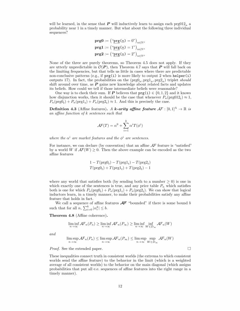
None of the three are purely theorems, so Theorem 4.5 does not apply. If theyare utterly unpredictable in O(P ), then Theorem 4.7 says that P will fall back onthe limiting frequencies, but that tells us little in cases where there are predictablenon-conclusive patterns (e.g., if prg(i) is more likely to output 2 when helper(i)outputs 17). In fact, the probabilities on the (prg0n,prg1n,prg2n) triplet shouldshift around over time, as P gains new knowledge about related facts and updatesits beliefs. How could we tell if those intermediate beliefs were reasonable?

One way is to check their sum. If P believes that prg(i) ∈ {0, 1, 2} and it knowshow disjunction works, then it should be the case that whenever Pn(prg012t) ≈ 1,Pn(prg0t) + Pn(prg1t) + Pn(prg2t) ≈ 1. And this is precisely the case.

Definition 4.3 (Affine features). A k-arity affine feature AF : [0, 1]Λ → R isan affine function of k sentences such that

AF(T ) = α0 +

k∑i=1

αiT (φi)

where the αi are market features and the φi are sentences.

For instance, we can declare (by convention) that an affine AF feature is “satisfied”by a world W if AF(W ) ≥ 0. Then the above example can be encoded as the twoaffine features

1− T (prg0t)− T (prg1t)− T (prg2t)

T (prg0t) + T (prg1t) + T (prg2t)− 1

where any world that satisfies both (by sending both to a number ≥ 0) is one inwhich exactly one of the sentences is true, and any price table Pn which satisfiesboth is one for which Pn(prg0t) + Pn(prg1t) + Pn(prg2t). We can show that logicalinductors learn, in a timely manner, to make their probabilities satisfy any affinefeature that holds in fact.

We call a sequence of affine features AF “bounded” if there is some bound b

such that for all n,∑ki=0 |αki | ≤ b.

Theorem 4.8 (Affine coherence).

lim infn→∞

AFn(Pn) ≥ lim infn→∞

AFn(P∞) ≥ lim infn→∞

infW∈D∞

AFn(W )

andlim supn→∞

AFn(Pn) ≤ lim supn→∞

AFn(P∞) ≤ lim supn→∞

supW∈D∞

AFn(W )

Proof. See the extended paper.

These inequalities connect truth in consistent worlds (the extrema to which consistentworlds send the affine feature) to the behavior in the limit (which is a weightedaverage of all consistent worlds) to the behavior on the main diagonal (which assignsprobabilities that put all e.e. sequences of affine features into the right range in atimely manner).

12

This doesn’t mean that P will solve difficult constraint satisfaction problemsin a timely manner, it just means P ’s probabilities will start respecting all linearinequalities in a timely manner. For example, if a set of complex constraints holdsbetween seven sequences of sentences, such that exactly three elements of eachseptuplet are true, but it’s difficult to figure out which three. Then P will learn thispattern, and start ensuring that its probabilities on each seven-tuple sum to 3, evenif it can’t yet assign particularly high probabilities to the correct three.

If we watch an individual seven-tuple as P reasons, other constraints will pushthe probabilities on those seven sentences up and down. One sentence might berefuted and have its probability go to zero. Another might get a boost when Pdiscovers that it’s implied by a high-probability sentence. Another might take ahit when P discovers it might imply a low-probability sentence. Throughout allthis, theorem 4.8 says that P will ensure that the seven probabilities always sum to≈ 3. P ’s beliefs on any given day arise from this interplay of theorem recognition,statistical pattern recognition, and the satisfaction of many different constraints,inductively learned.

In the extended version of this paper, we prove stronger and more general versionsof all the above results.

4.3 Self-knowledge

Logical inductors also learn to know what they know, and trust their future beliefs,in a way that avoids paradox. For starters,

Theorem 4.9 (Introspection). Let φφφ be an efficiently enumerable sequence ofsentences, a and b be efficiently enumerable sequences of probabilities, and δδδ be anefficiently enumerable sequence of positive real numbers. Define the sequence

ψψψ :=(

“an < Pn(φn) < bn”

)n∈N+

of sentences that say “the probability of φn on day n is in the interval (an, bn)”. Notethat ψψψ is e.e. (Pn need not be evaluated to produce ψn, it just needs to be writtendown). Then, for every ε > 0, the following two implications hold for all sufficientlylarge n:

1. if Pn(φn) ∈ (an + δn, bn − δn), then Pn(ψn) > 1− ε.

2. if Pn /∈ (an − δn, bn + δn), then Pn(ψn) < ε.

Proof. See the extended paper.

Roughly speaking, this says that if there is an e.e. pattern of the form “yourprobabilities on these sorts of sentences will be between (a, b)” then P will learn tobelieve that pattern iff it is true, subject to the caveat that its self-knowledge hasonly finite precision (i.e., if its beliefs are extremely close to a then it can’t alwaystell which side of a they are on).

This “finite-precision self-knowledge” allows logical inductors to avoid the classicparadoxes of self-reference:

Theorem 4.10 (Liar’s paradox resistance). Fix a rational p ∈ (0, 1), and define asequence of “liar sentences” Lp satisfying

Γ ` Lpn ↔(Pn(Lpn) < p

)for all n. (This can be done using, e.g., Godel’s diagonal lemma.) Then

limn→∞

Pn(Lpn) = p.

Proof. See the extended paper.

13

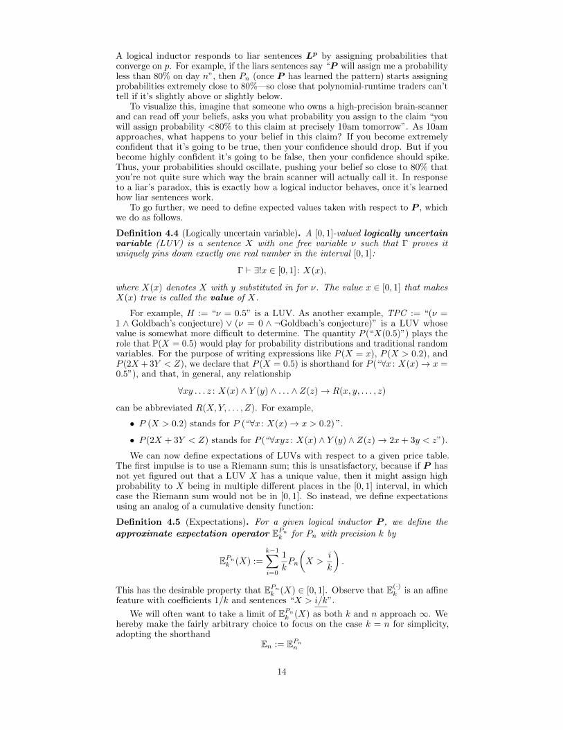
A logical inductor responds to liar sentences Lp by assigning probabilities thatconverge on p. For example, if the liars sentences say “P will assign me a probabilityless than 80% on day n”, then Pn (once P has learned the pattern) starts assigningprobabilities extremely close to 80%—so close that polynomial-runtime traders can’ttell if it’s slightly above or slightly below.

To visualize this, imagine that someone who owns a high-precision brain-scannerand can read off your beliefs, asks you what probability you assign to the claim “youwill assign probability <80% to this claim at precisely 10am tomorrow”. As 10amapproaches, what happens to your belief in this claim? If you become extremelyconfident that it’s going to be true, then your confidence should drop. But if youbecome highly confident it’s going to be false, then your confidence should spike.Thus, your probabilities should oscillate, pushing your belief so close to 80% thatyou’re not quite sure which way the brain scanner will actually call it. In responseto a liar’s paradox, this is exactly how a logical inductor behaves, once it’s learnedhow liar sentences work.

To go further, we need to define expected values taken with respect to P , whichwe do as follows.

Definition 4.4 (Logically uncertain variable). A [0, 1]-valued logically uncertainvariable (LUV) is a sentence X with one free variable ν such that Γ proves ituniquely pins down exactly one real number in the interval [0, 1]:

Γ ` ∃!x ∈ [0, 1] : X(x),

where X(x) denotes X with y substituted in for ν. The value x ∈ [0, 1] that makesX(x) true is called the value of X.

For example, H := “ν = 0.5” is a LUV. As another example, TPC := “(ν =1 ∧ Goldbach’s conjecture) ∨ (ν = 0 ∧ ¬Goldbach’s conjecture)” is a LUV whosevalue is somewhat more difficult to determine. The quantity P (“X(0.5)”) plays therole that P(X = 0.5) would play for probability distributions and traditional randomvariables. For the purpose of writing expressions like P (X = x), P (X > 0.2), andP (2X + 3Y < Z), we declare that P (X = 0.5) is shorthand for P (“∀x : X(x)→ x =0.5”), and that, in general, any relationship

∀xy . . . z : X(x) ∧ Y (y) ∧ . . . ∧ Z(z)→ R(x, y, . . . , z)

can be abbreviated R(X,Y, . . . , Z). For example,

• P (X > 0.2) stands for P (“∀x : X(x)→ x > 0.2) ”.

• P (2X + 3Y < Z) stands for P (“∀xyz : X(x) ∧ Y (y) ∧ Z(z)→ 2x+ 3y < z”).

We can now define expectations of LUVs with respect to a given price table.The first impulse is to use a Riemann sum; this is unsatisfactory, because if P hasnot yet figured out that a LUV X has a unique value, then it might assign highprobability to X being in multiple different places in the [0, 1] interval, in whichcase the Riemann sum would not be in [0, 1]. So instead, we define expectationsusing an analog of a cumulative density function:

Definition 4.5 (Expectations). For a given logical inductor P , we define the

approximate expectation operator EPnk for Pn with precision k by

EPnk (X) :=

k−1∑i=0

1

kPn

(X >

i

k

).

This has the desirable property that EPnk (X) ∈ [0, 1]. Observe that E(·)k is an affine

feature with coefficients 1/k and sentences “X > i/k”.

We will often want to take a limit of EPnk (X) as both k and n approach ∞. Wehereby make the fairly arbitrary choice to focus on the case k = n for simplicity,adopting the shorthand

En := EPnn

14

Observe that when n is finite, En can be interpreted as a market n-feature. Observethat each LUV X has a unique value in every consistent world, which means thateach X is a random variable (in the traditional sense) in the limit distribution P∞,and that E∞ is the usual expectation operator over P∞, where E∞(X) is a mixtureof the value of X in each consistent world (weighted according to P∞).

It is easy to show that expectations work as expected, for example:

Theorem 4.11 (Linearity of expectation). Let ααα and βββ be efficiently enumerablebounded sequences of n-market features. Let X,Y , and Z be efficiently enumerablesequences of LUVs. If for all n, Zn = αnXn + βnYn, then

αnEn(Xn) + βnEn(Yn) hn En(Zn).

Proof. See the extended paper.

Many other properties of the expectation operator are discussed in the extendedversion.

We can now show that logical inductors trust their future beliefs.

Theorem 4.12 (Conservation of Expected Updates). Let f : N+ → N+ be afunction with runtime polynomial in f(n), such that f(n) > n. Let φφφ denote an e.e.sequence of sentences.

Pn(φn) hn En(Pf(n)(φn)).

where En(Pf(n)(φn)) is shorthand for En(Xn) and Xn is the LUV “ν = P f(n)(φn)”.

Proof. See the extended paper.

Roughly speaking, this says that if P on day n believes that on day f(n) it willbelieve φn with high probability, then it already believes φn with high probabilitytoday. In other words, logical inductors learn to adopt their predicted future beliefsas their current beliefs in a timely manner—they don’t say “tomorrow I expect tobelieve that φ is true, but today I think it’s false”.

We will also show that, roughly speaking, logical inductors trust that if theirbeliefs change, then they must have changed for good reasons. To do this, we firstdefine:

[φ] := “(ν = 1 ∧ φ) ∨ (ν = 0 ∧ φ)”,

so that [φ] is the LUV with the value 1 if φ is true and false otherwise; and

[x ≥ p]δ := “ν =

0 if x < p(x− p

)/δ if p ≤ x ≤ p+ δ

1 if p+ δ < x.

”

so that [x ≥ p]δ is a LUV with the value 0 if x < p, 1 if x > p+ δ, and intermediatein between. Then

Theorem 4.13 (Self trust). Let φφφ be an e.e. sequence of sentences. Let δδδ be an e.e.sequence of positive rational numbers converging to zero. Let p be an e.e. sequenceof rational probabilities. Then

En([φn] · [Pf(n) (φn) ≥ pn]δn

)&n pn · En

([Pf(n) (φn) ≥ pn]δn

).

Proof. See the extended paper.

Roughly speaking, this says that if you ask P on day n for its belief in φ, conditionalon it believing on day f(n) that φ has probability p, it will answer with a probabilityat least p, regardless of whether or not its unconditional probability on p on day nis lower than p. In colloquial terms, conditional on its future beliefs changing, itexpects them to have changed for good reasons.

15

Notice that [Pf(n) (φn) ≥ pn]δn is a continuous indicator on P ’s future beliefs,which can be interpreted as saying that theorem 4.13 only holds when P has finite-precision access to its future beliefs. Indeed, theorem 4.13 breaks down if P getsinfinite-precision access to its future beliefs, and this is quite desirable. For example,let each φn be the liar sentence “P f(n)(φn) < 0.5” which says that the future

Pf(n) will assign probability less than 0.5 to the sentence. Then, conditional onPf(n)(φn) ≥ 0.5, Pn should believe that the probability of φn is 0. And indeed, thisis what a logical inductor will do:

Pn(“φn∧ (P f(n)(φn) ≥ 0.5)”) hn 0,

by a trivial application of theorem 4.7 (the limiting frequency of this sequence is 0,because each sentence is disprovable). This is why theorem 4.13 uses expectationsand fuzzy indicator functions: with discrete conjunctions, the result would beundesirable (and false).

Roughly speaking, theorem 4.13 says is that P attains self trust of the “if in thefuture I will believe x is very likely, then it must be because x is very likely” variety,if the conditional gives finite-precision access to its future beliefs. Simultaneously,P retains the ability to think it can outperform its future self’s beliefs given infinite-precision access to them. If you ask “what’s your probability on the liar sentenceφn given that your future self believes it with probability exactly 0.5?” then P willanswer “very low”, but if you ask “what’s your probability on the liar sentence φngiven that your future self believes it with probability extremely close to 0.5?” thenP will answer “roughly 0.5.”

In the extended version of this paper, we prove generalized versions of the aboveresults, and discuss a number of other subjects (such as calibration and conditionalprobabilities) in some depth.

5 Construction

We now give a computable algorithm for constructing a logical inductor.

5.1 Proof sketch

Imagine a reasoner writing out price tables at a rate of one per day, with theknowledge that those prices are going to be used to run a market full of polynomialtime traders, and that they will be obligated to buy and sell arbitrarily many sharesat the listed prices. If they can produce a sequence of price tables that satisfy thelogical induction criterion, then the resulting prices, interpreted as beliefs aboutlogic, will have the desirable properties listed above.

Our algorithm for doing this is easier to visualize if we begin with a finite case.First, notice that if there is a trader that exploits a market, then there is anothertrader that exploits the market while having their plausible worth bounded belowby -1 (simply scale down the trades of the first trader). Thus, in the finite setting,the reasoner can take all traders, give them each $1, and act as follows each day.First, run all traders to get their trade strategies. Second, cut their trades off if theygo over-budget. Third, combine all the strategies into a single net trading strategy,which is a continuous function from the day’s prices to a net trade, where the nettrade lists the net volume on all (finitely many) sentences that some trader mightbuy/sell shares on that day.

Now what the reasoner can do is search for a price table that causes the nettrade to be zero everywhere (or possibly causes net buy orders for shares priced at 1,or net sell orders for shares priced at 0). We will show that this can be done usingBrouwer’s fixed point theorem. If the net trade is zero everywhere, then for everyshare of φ bought by one trader, there’s a share of φ sold by other traders, and themoney in the system always gets shuffled around between traders, so the reasonernever puts any of their own money in. If the net trade purchases shares at price 1or sells at price 0, no money flows into the system. The prices that make the net

16

trades literally zero can be difficult to find, so we will have the reasoner approximatethose prices to within ε; the reasoner will cut ε in half each day, such that they onlyever have to put in at most $1 into their own market. Because the market startswith a finite amount of money (one dollar per trader for finitely many traders), andonly a finite amount of money is ever added, the plausible worth of every individualtrader must remain finite.

The situation gets a bit more complicated in the infinite case; we will do thefollowing. The reasoner will take one additional trader under consideration each day.They will spread out a single dollar among all the traders, in a way that ensures thatthe nth trader has at most 2−n wealth by the time they enter consideration. (Thiswill entail giving the nth trader less than 2−n to start, and setting aside a portionof the first dollar to cover trades that the nth trader makes before it is taken underconsideration). Then, each day, they will find a price table that causes the net tradevolume among all considered traders to be twice as close to zero as it was the daybefore. Thus, the market starts with a finite amount of money in it, and the marketwill only ever have a finite amount of money added to it, so the plausible wealth ofevery individual trader will be bounded above.

5.2 Proxy Traders

Fix an enumeration (t1, t2, . . .) of all traders. We begin by showing how to takethe ith trader and construct a proxy trader that (1) has their trades cut off if atrade would cause their plausible worth to dip below −2−i and (2) has their tradingstrategy scaled down so much that, on day i, their plausible worth is at most 2−i.

For each ti, we define the sequence of market features αααi recursively as follows.Each αin takes a market history P≤n as input and computes the maximum value in[0, 1] such that, for all W ∈ Dn,∑

j≤n

∑φ∈Λ

(αij(P≤j) · tij(φ)(P≤j)

)(W (φ)− Pj(φ)) ≥ −1.

Intuitively, αin calculates the amount to scale tin down to ensure that ti’s minimumworth on day n doesn’t dip below −1, according to any world W which is stillplausible to D on day n, and assuming that ti<n were scaled by αααi<n.

Observe that each αin is computable, because each tij is non-zero on only finitelymany sentences, so only finitely many combinations of truth values to those sentencesneed to be checked. (Recall that PlausibleDn can be used to check whether a certaintruth assignment remains plausible, and that it is computable.) However, thesequence αααi cannot necessarily be generated in polynomial time.

Next, for each ti, define

βi(P<i) :=2−i

max(

1,∑j<i α

ij(P≤j) · |tij(P≤j)|

)Multiplying all of ti’s trades by βi has two effects. First, it scales all trades down bya factor of at least 2i, ensuring that the plausible worth of the ith trader never dipsbelow −2−i. Second, notice that the denominator is the total trade volume of theith trader before day i (or 1, whichever is greater). Thus, multiplying every tradeby βi ensures that the worth of the trader on the ith day is at most 2−i, accordingto any world W ∈ Di.

Now, given a sequence of price tables P = (P1, P2, . . .) we can define a proxytrader xi for each trader ti:

xin(φ)(P≤n) := βi(P<i) · αin(P≤n) · tin(φ)(P≤n).

Observe that xi has the type of a trader, but is not a trader itself. Firstly, becauseP<i must be known before xin can be computed, even if n� i; and secondly, becauseαααi is not efficiently enumerable.

17

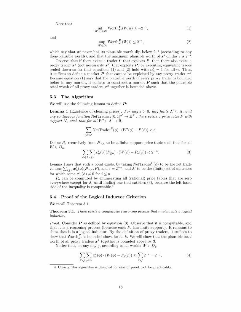
Note thatinf

(W,n)∈WWorthP

xi(W,n) ≥ −2−i, (1)

andsupW∈Di

WorthPxi(W, i) ≤ 2−i, (2)

which say that xi never has its plausible worth dip below 2−i (according to anythen-plausible worlds), and that the maximum plausible worth of xi on day i is 2−i.

Observe that if there exists a trader ti that exploits P , then there also exists aproxy trader xj (not necessarily xi) that exploits P , by executing equivalent tradesscaled down so far that equations (1) and (2) hold with αin = 1 for all n. Thus,it suffices to define a market P that cannot be exploited by any proxy trader xk.Because equation (1) says that the plausible worth of every proxy trader is boundedbelow in any market, it suffices to construct a market P such that the plausibletotal worth of all proxy traders xk together is bounded above.

5.3 The Algorithm

We will use the following lemma to define P :

Lemma 1 (Existence of clearing prices). For any ε > 0, any finite Λ′ ⊆ Λ, and

any continuous function NetTrades : [0, 1]Λ′ → RΛ′ , there exists a price table P with

support Λ′, such that for all W ′ ∈ Λ′ → B,∑φ∈Λ′

NetTradesP (φ) · (W ′(φ)− P (φ)) < ε.

Define Pn recursively from P<n to be a finite-support price table such that for allW ∈ Dn, ∑

φ∈Λ

∑i≤n

xin(φ)(P≤n) · (W (φ)− Pn(φ)) < 2−n. (3)

Lemma 1 says that such a point exists, by taking NetTradesP (φ) to be the net tradevolume

∑i≤n x

in(φ)(P<n, P ), and ε = 2−n, and Λ′ to be the (finite) set of sentences

for which some xin(φ) 6= 0 for i ≤ n.Pn can be computed by enumerating all (rational) price tables that are zero

everywhere except for Λ′ until finding one that satisfies (3), because the left-handside of the inequality is computable.4

5.4 Proof of the Logical Inductor Criterion

We recall Theorem 3.1:

Theorem 3.1. There exists a computable reasoning process that implements a logicalinductor.

Proof. Consider P as defined by equation (3). Observe that it is computable, andthat it is a reasoning process (because each Pn has finite support). It remains toshow that it is a logical inductor. By the definition of proxy traders, it suffices toshow that WorthP

xk is bounded above for all k. We will show that the plausible totalworth of all proxy traders xk together is bounded above by 3.

Notice that, on any day j, according to all worlds W ∈ Dj ,∑i>j

∑φ∈Λ

xij(φ) · (W (φ)− Pj(φ)) ≤∑i>j

2−i = 2−j , (4)

4. Clearly, this algorithm is designed for ease of proof, not for practicality.

18

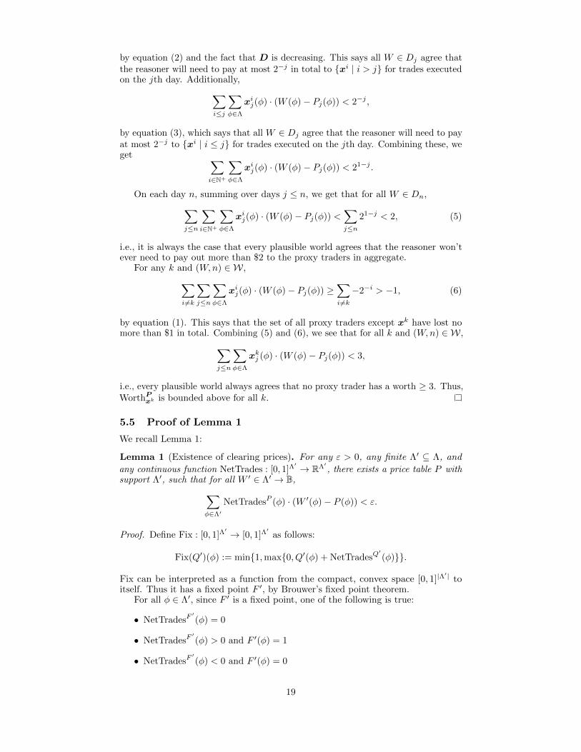
by equation (2) and the fact that D is decreasing. This says all W ∈ Dj agree thatthe reasoner will need to pay at most 2−j in total to {xi | i > j} for trades executedon the jth day. Additionally,∑

i≤j

∑φ∈Λ

xij(φ) · (W (φ)− Pj(φ)) < 2−j ,

by equation (3), which says that all W ∈ Dj agree that the reasoner will need to payat most 2−j to {xi | i ≤ j} for trades executed on the jth day. Combining these, weget ∑

i∈N+

∑φ∈Λ

xij(φ) · (W (φ)− Pj(φ)) < 21−j .

On each day n, summing over days j ≤ n, we get that for all W ∈ Dn,∑j≤n

∑i∈N+

∑φ∈Λ

xij(φ) · (W (φ)− Pj(φ)) <∑j≤n

21−j < 2, (5)

i.e., it is always the case that every plausible world agrees that the reasoner won’tever need to pay out more than $2 to the proxy traders in aggregate.

For any k and (W,n) ∈ W,∑i 6=k

∑j≤n

∑φ∈Λ

xij(φ) · (W (φ)− Pj(φ)) ≥∑i6=k

−2−i > −1, (6)

by equation (1). This says that the set of all proxy traders except xk have lost nomore than $1 in total. Combining (5) and (6), we see that for all k and (W,n) ∈ W ,∑

j≤n

∑φ∈Λ

xkj (φ) · (W (φ)− Pj(φ)) < 3,

i.e., every plausible world always agrees that no proxy trader has a worth ≥ 3. Thus,WorthP

xk is bounded above for all k.

5.5 Proof of Lemma 1

We recall Lemma 1:

Lemma 1 (Existence of clearing prices). For any ε > 0, any finite Λ′ ⊆ Λ, and

any continuous function NetTrades : [0, 1]Λ′ → RΛ′ , there exists a price table P with

support Λ′, such that for all W ′ ∈ Λ′ → B,∑φ∈Λ′

NetTradesP (φ) · (W ′(φ)− P (φ)) < ε.

Proof. Define Fix : [0, 1]Λ′ → [0, 1]Λ

′as follows:

Fix(Q′)(φ) := min{1,max{0, Q′(φ) + NetTradesQ′(φ)}}.

Fix can be interpreted as a function from the compact, convex space [0, 1]|Λ′| to

itself. Thus it has a fixed point F ′, by Brouwer’s fixed point theorem.For all φ ∈ Λ′, since F ′ is a fixed point, one of the following is true:

• NetTradesF′(φ) = 0

• NetTradesF′(φ) > 0 and F ′(φ) = 1

• NetTradesF′(φ) < 0 and F ′(φ) = 0

19

It follows that NetTradesF′(φ) · (W ′(φ)−F ′(φ)) ≤ 0 for all φ ∈ Λ′ and W ′ : Λ′ → B.

F ′ is almost the price table we need, except that it is not necessarily rational.However, ∑

φ∈Λ′

NetTradesQ′(φ) · (W ′(φ)−Q′(φ))

is continuous in Q′, so for any ε > 0 there is some rational P ′ : Λ′ → [0, 1] closeenough to F ′ such that for all W ′ : Λ′ → B,∑

φ∈Λ′

NetTradesP′(φ) · (W ′(φ)− P ′(φ)) < ε.

Define P (φ) to be P ′(φ) if φ ∈ Λ′ and 0 otherwise.

6 Selected proofs

In this section, we will prove theorems 4.1, 4.2, and 4.7. The remaining proofs (andproofs of many other properties) can be found in the extended version of the paper.

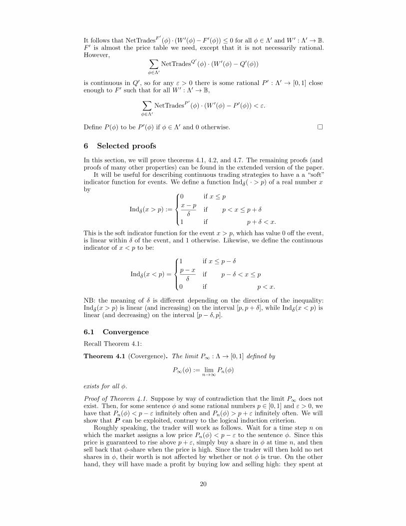
It will be useful for describing continuous trading strategies to have a a “soft”indicator function for events. We define a function Indδ( · > p) of a real number xby

Indδ(x > p) :=

0 if x ≤ px− pδ

if p < x ≤ p+ δ

1 if p+ δ < x.

This is the soft indicator function for the event x > p, which has value 0 off the event,is linear within δ of the event, and 1 otherwise. Likewise, we define the continuousindicator of x < p to be:

Indδ(x < p) =

1 if x ≤ p− δp− xδ

if p− δ < x ≤ p

0 if p < x.

NB: the meaning of δ is different depending on the direction of the inequality:Indδ(x > p) is linear (and increasing) on the interval [p, p+ δ], while Indδ(x < p) islinear (and decreasing) on the interval [p− δ, p].

6.1 Convergence

Recall Theorem 4.1:

Theorem 4.1 (Covergence). The limit P∞ : Λ→ [0, 1] defined by

P∞(φ) := limn→∞

Pn(φ)

exists for all φ.

Proof of Theorem 4.1. Suppose by way of contradiction that the limit P∞ does notexist. Then, for some sentence φ and some rational numbers p ∈ [0, 1] and ε > 0, wehave that Pn(φ) < p− ε infinitely often and Pn(φ) > p+ ε infinitely often. We willshow that P can be exploited, contrary to the logical induction criterion.

Roughly speaking, the trader will work as follows. Wait for a time step n onwhich the market assigns a low price Pn(φ) < p − ε to the sentence φ. Since thisprice is guaranteed to rise above p+ ε, simply buy a share in φ at time n, and thensell back that φ-share when the price is high. Since the trader will then hold no netshares in φ, their worth is not affected by whether or not φ is true. On the otherhand, they will have made a profit by buying low and selling high: they spent at

20

most p− ε buying a φ-share, and then made at least p+ ε selling a φ-share. Sincethe prices Pn(φ) fluctuate forever, they will continue making money forever andthus exploit the market.

We will define a trader t that executes a strategy similar to this one, and henceexploits the market P if limn→∞ Pn(φ) does not converge. To do this, there aretwo technicalities we must deal with. First is that the strategy outlined above is adiscontinuous function of the market prices Pn(φ), and therefore is not permitted.This is relatively easy to fix using soft indicator functions described above.

The second technicality is more subtle. Suppose we define our trader to buyφ-shares whenever their price Pn(φ) is low, and sell them back whenever their priceis high. Then it is possible that the trader makes the following trades in sequenceagainst the market P : buy 10 φ-shares on consecutive days, then sell 10 φ-shares;then buy 100 φ-shares consecutively, and then sell them off; then buy 1000 φ-shares,then sell them off; and so on. Although this trader makes profit on each batch, italways spends more on the next batch, taking larger and larger risks (relative tothe remaining plausible worlds). In short, this trader is not tracking its budget,and so may have unboundedly negative Worth. We will fix this problem by havingour trader t track how many net φ-shares it has bought, and not buying too many,thereby maintaining bounded risk. This will be sufficient to prove the theorem.

Definition of the trader t Let the quantity

Sharesφn :=∑i<n

ti(φ)

denote the total net number of φ-shares that t has purchased before the currenttime n. Now we define the trader t to output the trading strategy tn on time ndefined by

tn(φ) := (1− Sharesφn)× Indε/2(Pn(φ) < p− ε/2)

− Sharesφn × Indε/2(Pn(φ) > p+ ε/2),

and tn(γ) := 0 for other sentences γ 6= φ. Note that tn is computable with runtimepolynomial in n. Furthermore, the trading strategies tn assign a single marketn-feature to φ, as required; thus t is a well-defined trader.5

In words, t buys some φ-shares whenever Pn(φ) < p− ε/2, up to 1 share whenPn(φ) < p − ε; and sells some φ-shares whenever Pn(φ) > p + ε/2, up to 1 share

when Pn(φ) > p+ ε. These trades are scaled down according to the number Sharesφnof φ-shares t has bought in total. If t has bought a full φ-share to date that has notbeen balanced out by selling a φ-share, then 1− Sharesφn = 0, so t will not buy any

more φ-shares; and Sharesφn = 1, so if given the opportunity t would sell up to a fullshare in φ. Likewise, if t has bought 0 net shares in φ to date, then it will buy upto 1 full φ-share if given the opportunity by a low market price Pn(φ), but will notsell any shares in φ. Thus we have shown that for any time step n, our trader t haspurchased a net total of Sharesφn ∈ [0, 1] shares in φ.

Analyzing WorthPt . We will now lower bound the Worth of t against the market

P over the deductive process D.In words: we focus just on φ-shares, as t doesn’t trade on other sentences. As

time goes on, since Sharesφn ∈ [0, 1], t holds at most 1 net share in φ. Thus thepayouts and the costs from the surplus φ-shares held by t contribute little to the totalprofit. If t has bought k/2 shares and sold k/2 shares in φ, then by the definition ofwhen t buys and sells, t has made a profit of a least (k/2)(p+ε/2−(p−ε/2)) = kε/2.The payouts from those φ-shares cancel each other out.

5. Note that t is defined making reference to the values of its previous trades ti(φ). Thiscan be done efficiently in general, by computing t’s past trades inside t’s trading strategyusing dynamic programming. For details, see the extended paper.

21

Formally, for any time n and any world W ∈ Dn,

WorthPt (W,n) :=

∑i≤n

∑ψ∈Λ

ti(ψ) · (W (ψ)− Pi(ψ))

=∑i≤n

ti(φ) · (W (φ)− Pi(φ))

since t only makes non-zero trades on φ;

=(

Sharesφn+1 ·W (φ))−∑i≤n

ti(φ) · Pi(φ)

since t holds Sharesφn-many net φ-shares;

≥ Sharesφn+1 · 0 +∑i≤n

Pi(φ)<p−ε/2

ti(φ) · (−Pi(φ))

+∑i≤n

Pi(φ)>1+ε/2

(−ti(φ)) · Pi(φ)

≥∑i≤n

Pi(φ)<p−ε/2

ti(φ) · (−(p− ε/2))

+∑i≤n

Pi(φ)>p+ε/2

(−ti(φ)) · (p+ ε/2)

since ti(φ) > 0 iff Pi(φ) < 1− ε/2, and ti(φ) < 0 iff Pi(φ) > 1 + ε/2;

=∑i≤n

|ti(φ)| · ε/2−∑i≤n

ti(φ) · p

=∑i≤n

|ti(φ)| · ε/2− Sharesφn+1 · p

≥ −p+∑i≤n

|ti(φ)| · ε/2.

Thus, the worth of t at time n is roughly ε/2 times the total trading volume |t≤n|up until time n. In particular, WorthP

t is bounded below by −p. Futhermore, bysupposition, Pi(φ) < 1− ε and then Pj(φ) > 1 + ε for infinitely many i and infinitelymany j > i. But that means that infinitely often, our trader t will have purchased afull φ-share (i.e. Sharesφn = 1), and then sold back a full φ-share (i.e. Sharesφn = 0),and so on, making ε/2 profit each time.

That is, the sum∑i≤n |ti(φ)| diverges to∞ as n→∞. Thus t has worth against

P lower bounded but not upper bounded, and therefore exploits the market P . Thiscontradicts that P is a logical inductor; therefore, in fact the limit P∞(φ) mustexist.

6.2 Limit Coherence

Recall Theorem 4.2:

Theorem 4.2 (Limit Coherence). P∞ is coherent, i.e., it gives rise to an internallyconsistent probability measure P on the set D∞ of all worlds consistent with Γ,defined by the formula

P(W (φ) = 1) := P∞(φ).

In other words, P∞ is a probability measure on the set of completions of Γ.

22

Proof of Theorem 4.2. By Convergence (Theorem 4.1), the limit P∞(φ) exists forall sentences φ ∈ Λ. Therefore, P(W (φ) = 1) := P∞(φ) is well-defined as a functionof basic subsets of D∞.

Gaifman (1964) shows that P extends to a probability measure over D∞ so longas the following three implications hold for all sentences φ an ψ:

• If Γ ` φ, then P∞(φ) = 1.

• If Γ ` ¬φ, then P∞(φ) = 0.

• If Γ ` ¬(φ ∧ ψ), then P∞(φ ∨ ψ) = P∞(φ) + P∞(ψ).

Since the three conditions are quite similar in form, we will prove them simultaneouslyusing three exemplar traders and parallel arguments.

Suppose for contradiction that one of these implications fails to hold by someamount ε. For example, suppose that P∞(φ∨ψ) = P∞(φ) +P∞(ψ)−ε, even thoughΓ proves that ¬(φ ∧ ψ). Intuitively, shares in φ ∨ ψ are underpriced by around ε. Ifwe wait for Pn to approximately converge, and then buy a (φ ∨ ψ)-share and sell aφ-share and a ψ-share, we have made a profit of about ε. We will have to pay outon at most one of the φ-share and the ψ-share, and if we do, we will also recieve apayout from the (φ ∨ ψ)-share. In this way we can exploit the market P repeatedly,for unbounded gains at no risk.

Definition of the traders tφ, tψ, tφ∨ψ≥, and tφ∨ψ≤. Suppose that one of thethree conditions is violated by ε, i.e.

• Γ ` φ, but P∞(φ) < 1− ε.• Γ ` ¬φ, but P∞(φ) > ε.

• Γ ` ¬(φ ∧ ψ), but P∞(φ ∨ ψ) < P∞(φ) + P∞(ψ)− ε.• Γ ` ¬(φ ∧ ψ), but P∞(φ ∨ ψ) > P∞(φ) + P∞(ψ) + ε.

Since the limit P∞ exists, there is some sufficiently large time sε such that for alln > sε, the inequality holds for Pn; e.g., for all n > sε, Pn(φ∨ψ) > Pn(φ)+Pn(ψ)+ε.

Furthermore, since D is a Γ-valid deductive process, for some sufficiently largesΓ and all n > sΓ, all worlds W in the deductive state Dn satisfy the appropriatelogical constraint on the sentences φ and ψ. For example, eventually all plausibleworlds assign 0 to φ if Γ ` ¬φ; and if Γ ` ¬(φ∧ψ), then eventually all worlds assign1 to at most one of φ and ψ, and if either are assigned 1 then so is φ ∨ ψ.

Let s := max{sε, sΓ}. We now define traders that will exploit the market P .All of the following traders will make no non-zero trades for n ≤ s, and will makenon-zero trades only for the sentences explicitly mentioned. For n > s, we define

tφn(φ) := 1

to be the trader tφ that attempts to ensure P∞(φ) = 1 by buying φ-shares;

t¬φn (φ) := −1

to be the trader t¬φ that attempts to ensure P∞(φ) = 0 by selling φ-shares;

tφ∨ψ≥n (φ) := −1

tφ∨ψ≥n (ψ) := −1

tφ∨ψ≥n (φ ∨ ψ) := 1

to be the trader tφ∨ψ≥ that attempts to ensure P∞(φ ∨ ψ) ≥ P∞(φ) + P∞(ψ); and

tφ∨ψ≤n (φ) := 1

tφ∨ψ≤n (ψ) := 1

tφ∨ψ≤n (φ ∨ ψ) := −1

to be the trader tφ∨ψ≤ that attempts to ensure P∞(φ∨ψ) ≤ P∞(φ)+P∞(ψ). Thesetraders all run in constant time; the constant s can be hard-coded at constant cost.

23

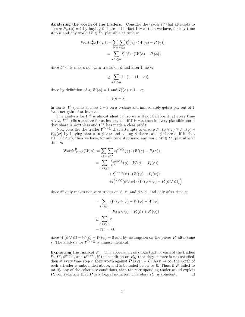
Analyzing the worth of the traders. Consider the trader tφ that attempts toensure P∞(φ) = 1 by buying φ-shares. If in fact Γ ` φ, then we have, for any timestep n and any world W ∈ Dn plausible at time n:

WorthPtφ(W,n) :=

∑i≤n

∑γ∈Λ

tφi (γ) · (W (γ)− Pi(γ))

=∑s<i≤n

tφi (φ) · (W (φ)− Pi(φ))

since tφ only makes non-zero trades on φ and after time s;

≥∑s<i≤n

1 · (1− (1− ε))

since by definition of s, W (φ) = 1 and Pi(φ) < 1− ε;

= ε(n− s).

In words, tφ spends at most 1− ε on a φ-share and immediately gets a pay out of 1,for a net gain of at least ε.

The analysis for t¬φ is almost identical, so we will not belabor it; at every timen > s, t¬φ sells a φ-share for at least ε, and if Γ ` ¬φ, then in every plausible worldthat share is worthless and t¬φ has made a clear profit.

Now consider the trader tφ∨ψ≥ that attempts to ensure P∞(φ ∨ ψ) ≥ P∞(φ) +P∞(ψ) by buying shares in φ ∨ ψ and selling φ-shares and ψ-shares. If in factΓ ` ¬(φ ∧ ψ), then we have, for any time step nand any world W ∈ Dn plausible attime n:

WorthPtφ∨ψ≥(W,n) :=

∑i≤n

∑γ∈Λ

tφ∨ψ≥i (γ) · (W (γ)− Pi(γ))

=∑s<i≤n

(tφ∨ψ≥i (φ) · (W (φ)− Pi(φ))

+ tφ∨ψ≥i (ψ) · (W (ψ)− Pi(ψ))

+tφ∨ψ≥i (φ ∨ ψ) · (W (φ ∨ ψ)− Pi(φ ∨ ψ)))

since tφ only makes non-zero trades on φ, ψ, and φ ∨ ψ, and only after time s;

=∑s<i≤n

(W (φ ∨ ψ)−W (φ)−W (ψ)

−Pi(φ ∨ ψ) + Pi(φ) + Pi(ψ))

≥∑s<i≤n

ε

= ε(n− s),

since W (φ ∨ ψ)−W (φ)−W (ψ) = 0 and by assumption on the prices Pi after times. The analysis for tφ∨ψ≤ is almost identical.

Exploiting the market P . The above analysis shows that for each of the traderstφ, tψ, tφ∨ψ≥, and tφ∨ψ≤, if the condition on P∞ that they enforce is not satisfied,then at every time step n their worth against P is ε(n− s). As n→∞, the worth ofsuch a trader is unbounded above, and is bounded below by 0. Thus, if P failed tosatisfy any of the coherence conditions, then the corresponding trader would exploitP , contradicting that P is a logical inductor. Therefore P∞ is coherent.

24

6.3 Learning Pseudorandom Frequencies

Recall Theorem 4.7:

Theorem 4.7 (Learning pseudorandom frequencies). Let φφφ be an e.e. sequence ofΓ-decidable sentences which is p-pseudorandom over O(P ). Then

Pn(φn) hn p.

Proof of Theorem 4.7. Assume the theorem did not hold. Then, intuitively, Prepeatedly underprices the φn. A trader can buy φn-shares whenever their price goesbelow p− ε. By the assumption that the truth values of the φn are pseudorandom,roughly p proportion of the shares will pay out. Since the trader only pay at mostp− ε per share, on average they make ε on each trade, so over time we exploit themarket.

We will have to make these trades continuous. Furthermore, as in the proof ofTheorem 4.1, we will need to budget our trader to prevent it from investing moreand more in sentences φn that may take a very long time to pay out.

Suppose for contradiction that φφφ is an e.e. sequence of Γ-decidable sentencessuch that for every practical fuzzy subset f ,

limn→∞

∑i<n f(i) · [Γ ` φi]∑

i<n f(i)= p;

but nevertheless, for some ε > 0 and infinitely many n, we have (say)

Pn(φn) < p− ε.

(The argument for the case where Pn(φn) > p+ ε infinitely often will be the same,mutatis mutandis, and one of these two cases must obtain.)

Definition of the trader t. Say that a sentence φ is settled at time n if everyworld W ∈ Dn assigns the same value to φ. Because D is Γ-valid and everyφn is decidable, every φn is eventually settled. Since the deductive process D iscomputable, there is a function S : Λ→ N+ → {0, 1}, computable in time polynomialin n, that approximates the set of sentences by assigning 0 to settled sentences and1 to possibly unsettled sentences. That is,

• for any φ and any n, if S(n, φ) = 0 then φ is settled at time n;• for any φ and any m > n, if S(n, φ) = 0 then S(m,φ) = 0; and• for any φ, for some sufficiently large n, S(n, φ) = 0.

Note that S may assign 1 to settled sentences (this allows S to be efficiently computed,even if the deductive process D is not).

Our trader t will never have more than one share unsettled at any given time,in order to avoid going into debt by purchasing ever more unsettled investments.Formally, we define

βn := 1−∑i<n

S(φi, n)ti(φi)

to be the fraction of t’s budget of 1 that is not tied up in possibly unsettled φi-shares.Then we define t at time n to be

tn(φn) := βn Indε/2(Pn(φn) < p− ε/2),

and tn(γ) := 0 for other sentences γ 6= φ. Note that this tn can be computed inpolynomial time in n, using S. 6 In words, tn uses some fraction of its free budgetβn to buy φn-shares, depending on to what extent they are priced below p− ε/2. Inparticular, all the βn and all the tn(φ) are in [0, 1].

6. As mentioned in a previous footnote, t is defined using the values of its previoustrades ti(φ); this can be implemented efficiently.

25

t is a practical fuzzy subset. Now we show that the sequence of trades tn(φn)made by our trader t against the market P forms a practical fuzzy subset. Since tis efficiently computable and tn(φn) ∈ [0, 1] for all n, it remains to show that∑

n

tn(φn) =∞.

That is, we want to show that tmades trades will unbounded total volume. Intuitively,every trade that t makes is eventually settled according to S, after which point βn islarge again, and t continues buying φn-shares whenever Pn(φn) < p− ε/2. Formally,suppose this were not the case, so that for some sufficiently large m,∑

n>m

tn(φn) < 1/2.

Then by definition of S, for some sufficiently large m′, S(φi,m′) = 0 for all i ≤ m.

At that point, for any n > m′, we have

βn := 1−∑i<n

S(φi, n)ti(φi)

1−∑

m′<i<n

S(φi, n)ti(φi)

≥ 1/2.

Then, by the earlier supposition on P , for some n > m′ we have Pn(φn) < p− ε, atwhich point

tn(φn) := βn Indε/2 = (Pn(φn) < p− ε/2) ≥ 1/2.

This contradicts the supposition that∑n tn(φn) is bounded, so in fact the sum is

infinite as desired, i.e. t is a practical fuzzy subset.

Analyzing the worth of t. Now, by definition of φφφ being a pseudorandomsequence, we have that

limn→∞

∑i<n ti(φi) · [Γ ` φi]∑

i<n ti(φi)= p.

Thus, for all sufficiently large n,∑i<n

ti(φi) · [Γ ` φi] ≥ (p− ε/4)∑i<n

ti(φi).

The sum on the left is, roughly, the value of all the φi-shares held by t before timen, and the sum on the right is the total number of shares purchased by t. Indeed,at time n, all but at most 1 of the shares held by t has been settled, so there is adiscrepancy on the left hand side of at most 1.

By definition of t, the total price paid by t for its purchases before time n is atmost ∑

i<n

ti(φi)(p− ε/2).

Thus, the total worth of t against the market P before time n is at least

−1 + (p− ε/4− (p− ε/2))∑i<n

ti(φi) 'n (ε/4)∑i<n

ti(φi).

Thus WorthPt (W,n) is bounded below. Further, since t makes trades of unbounded

volume, i.e.∑n tn(φn) = ∞, WorthP

t (W,n) grows unboundedly. Therefore texploits the market P . This contradicts that P is a logical inductor, so in fact wemust have that

limn→∞

Pn(φn) = p.

26

7 Discussion

We have proposed the logical induction criterion as a criterion for beliefs aboutlogical facts (represented explicitly as a series of price tables), and demonstrated thatlogical inductors have many desirable properties when it comes to reasoning aboutlogical facts. For example, logical inductors learn (in a timely manner) to assignprobabilities near 1 to any sequence of theorems that can be produced in polynomialtime, which often requires outpacing the underlying deductive process. Similarly,logical inductors learn to assign probabilities near 0 to all efficiently enumerablesequences of contradictions, and they learn to assign probabilities that respect linearinequalities that will hold in the limit (such as ensuring that the probabilities of“prg(i)=0” and “prg(i)=1” sum to no more than 1, and so on), and they learn tofall back on appropriate statistical summaries in the face of pseudorandom sequences.They also learn to know their current beliefs and trust their future beliefs, and theirbeliefs are fully coherent in the limit.

We have presented a computable algorithm that demonstrates that it is possibleto meet the logical induction criterion. Clearly, the algorithm presented in Section 5is not intended for practical use. On the contrary, logical induction is intended toserve as a theoretical account of how to learn inductively to predict unknown logicalfacts (such as the behavior of a long-running computer program) from known ones(such as the observation of shorter-running computer programs). In this way, it isanalogous to Solomonoff’s theory of inductive inference (Solomonoff 1964), whichprovides a theoretical account of how to use Bayesian probability theory to learninductively to predict unknown empirical facts (the next observation that will beproduced by an environment) from known ones (the history of observations producedby the environment).

As an analogy, in the field of artificial intelligence (AI), Bayesian probabilitytheory has provided inspiration for a wide array of AI algorithms, from BeliefPropagation (Pearl 1988) to Auto-Encoding Variational Bayes (Kingma and Welling2013). Indeed, while perfect Bayesian reasoning is intractable in practice, the idiomof representing beliefs with probabilities and responding to evidence in an approxi-mately Bayesian fashion is ubiquitous throughout the field of AI. Similarly, whileSolomonoff’s theory of inductive inference is uncomputable, the idea of consulting aset of experts, rewarding them for predicting the data well, and penalizing them forcomplexity, is a ubiquitous idiom for predictive analytics. Logical induction aspiresto provide an analogous theoretical foundation for algorithms that are predictinglogical facts (such as the behavior of computations that are too expensive to run).

The authors are particularly interested in tools that help AI scientists attainnovel robustness and reliability guarantees in settings where statistical guaranteesare currently hard to come by. This includes settings where AI systems have toreason about computations that are too expensive to run, as discussed by Fallensteinand Soares (2015), and also settings where AI systems have to reason about otheragents that are logically uncertain. For example, consider an AI system attemptingto learn a human’s goals, and imagine it observing the human make a losing chessmove. Such a system should not conclude that the human wanted to lose; it shouldinstead have a model of the human being logically uncertain, with beliefs constrainedby deductive limitations. (For further discussion on this topic, refer to Russell [2014]and Li et al. [2010].) In settings such as these, we expect logical induction to helpby providing an early theoretical framework for studying deductively limited (butotherwise rational) reasoners.

The authors believe that the logical induction criterion captures a sizable portionof what it means to manage uncertainty well in the face of deductive limitations, inthe same way that the “no Dutch book” criteria of Ramsey (1931) and de Finetti(1979) capture a sizable portion of what it means to manage uncertainty well in theface of empirical uncertainty. Roughly speaking, logical inductors learn to recognizeall patterns that can be found in polynomial time; and any reasoning process thatdoes not satisfy the logical inductor criterion can (by definition) be exploited bysome stock trader that runs in polynomial time.

Nevertheless, logical induction leaves a number of questions wide open. For

27

example, logical induction does not obviously give good answers to questions aboutcounterpossibles, such as “what would math be like if Fermat’s last theorem werefalse?” While these questions may seem ridiculous at first glance, they are importantwhen it comes to developing a decision theory that is suitable for deductivelylimited reasoners, where one may want to ask “what will happen in the world ifagent(n)=action3?” and have some confidence that the answer will be reasonableeven if agent(n) does not in fact equal action3.

Finally, there is the question of whether logical inductors behave well in practice.One key insight of the algorithm in Section 5 is that it is possible for a limitedreasoner to construct reasonable beliefs about logical facts by consulting a collectionof “stock traders”, where each trader watches for (and attempts to profit from) acertain type of price inefficiency when the beliefs are interpreted as a price table.“Reasonable” beliefs (relative to a collection of traders) are then any prices that makethe market clear. The authors expect that algorithms which use these ideas—i.e.,by reasoning about a limited set of logical facts, running a finite collection of linear-time traders, and using standard gradient descent techniques to find approximatelyreasonable prices—can likely achieve good performance in practice. This is anempirical conjecture, which remains to be tested.

References

Aaronson, Scott. 2013. “Why Philosophers Should Care About Computational Complexity.”Chap. 10 in Computability: Turing, Godel, Church, and Beyond, edited by B. JackCopeland, Carl J. Posy, and Oron Shagrir, 261–328. Cambridge: MIT Press.

Campbell-Moore, Catrin. 2015. “How to Express Self-Referential Probability. A KripkeanProposal.” The Review of Symbolic Logic 8 (04): 680–704.

Carnap, Rudolf. 1962. Logical Foundations of Probability. Chicago, IL, USA: University ofChicago Press.

Christiano, Paul. 2014. Non-Omniscience, Probabilistic Inference, and Metamathematics.Technical report 2014–3. Berkeley, CA: Machine Intelligence Research Institute. http://intelligence.org/files/Non-Omniscience.pdf.

De Finetti, Bruno. 1979. Theory of Probability. New York, NY, USA: John Wiley & Sons.

Demski, Abram. 2012. “Logical Prior Probability.” In Artificial General Intelligence: 5thInternational Conference, AGI 2012, 50–59. Lecture Notes in Artificial Intelligence 7716.New York: Springer.

Fagin, Ronald, Yoram Moses, Moshe Y. Vardi, and Joseph Y. Halpern. 1995. ReasoningAbout Knowledge. Cambridge: MIT Press.

Fallenstein, Benja, and Nate Soares. 2015. Vingean Reflection: Reliable Reasoning forSelf-Improving Agents. Technical report 2015–2. Berkeley, CA: Machine IntelligenceResearch Institute. https://intelligence.org/files/VingeanReflection.pdf.

Gaifman, Haim. 1964. “Concerning Measures in First Order Calculi.” Israel Journal ofMathematics 2 (1): 1–18.

Good, Irving John. 1950. Probability and the Weighing of Evidence. London: Charles Griffin.

Hacking, Ian. 1967. “Slightly More Realistic Personal Probability.” Philosophy of Science34 (4): 311–325.

Hay, Nicholas, Stuart J. Russell, Solomon Eyal Shimony, and David Tolpin. 2012. “SelectingComputations: Theory and Applications.” In Uncertainty in Artificial Intelligence(UAI-’12), edited by Nando de Freitas and Kevin Murphy, 346–355.

Hintikka, Jaakko. 1962. Knowledge and Belief. Ithaca, N.Y.: Cornell University Press.

. 1975. “Impossible Possible Worlds Vindicated.” Journal of Philosophical Logic 4(4): 475–484.

Hutter, Marcus, John W. Lloyd, Kee Siong Ng, and William T. B. Uther. 2013. “Probabilitieson Sentences in an Expressive Logic.” Journal of Applied Logic 11 (4): 386–420.

28

Kingma, Diederik P., and Max Welling. 2013. “Auto-Encoding Variational Bayes.” arXiv:1312.6114 [stat.ML].

Levin, Leonid A. 1974. “Laws of Information Conservation (Nongrowth) and Aspects ofthe Foundation of Probability Theory.” Problemy Peredachi Informatsii (3): 30–35.

Li, Nan, William Cushing, Subbarao Kambhampati, and Sungwook Yoon. 2010. “Learningprobabilistic hierarchical task networks to capture user preferences.” arXiv preprintarXiv:1006.0274.

Pearl, Judea. 1988. Probabilistic Reasoning in Intelligent Systems: Networks of PlausibleInference. San Mateo, CA: Morgan Kaufmann.

Ramare, Olivier. 1995. “On snirel’man’s constant.” Annali della Scuola Normale Superioredi Pisa-Classe di Scienze 22 (4): 645–706.

Ramsey, Frank Plumpton. 1931. “Truth and Probability.” In The Foundations of Mathe-matics and other Logical Essays, edited by Richard Bevan Braithwaite, 156–198. NewYork: Harcourt, Brace.

Rantala, Veikko. 1975. “Urn Models: A New Kind of Non-Standard Model for First-OrderLogic.” Journal of Philosophical Logic 4 (4): 455–474.

Russell, Stuart J. 2014. “Unifying Logic and Probability: A New Dawn for AI?” InInformation Processing and Management of Uncertainty in Knowledge-Based Systems:15th International Conference IPMU 2014, Part I, 442:10–14. Communications inComputer and Information Science, Part 1. Springer.

Savage, Leonard J. 1967. “Difficulties in the theory of personal probability.” Philosophy ofScience 34 (4): 305–310.

Solomonoff, Ray J. 1964. “A Formal Theory of Inductive Inference. Part I.” Informationand Control 7 (1): 1–22.

Von Neumann, John, and Oskar Morgenstern. 1944. Theory of Games and EconomicBehavior. 1st ed. Princeton, NJ: Princeton University Press.

29