LOG MOISTURE CONTENT DETERMINATION WITH …

LOG MOISTURE CONTENT DETERMINATION WITH QUANTITATIVE

MAGNETIC RESONANCE

by

Clevan Reyve G. Lamason

Bachelor of Science in Forest Products Engineering, University of the Philippines Los

Baños, 1999

Master of Science in Forest Engineering, University of New Brunswick, 2006

A Dissertation Submitted in Partial Fulfillment

of the Requirements for the Degree of

Doctor of Philosophy

in the Graduate Academic Unit of Forestry and Environmental Management

Supervisors: Brigitte Leblon, Ph.D., Forestry and Environmental Management

Bruce J. Balcom, Ph.D., Physics

Examining Board: Igor Mastikhin, Ph.D., Department of Physics

Rod Stirling, Ph.D., Forestry & Environmental Management

Joseph Nader, Ph.D., Forestry & Environmental Management

External Examiner: Ian D. Hartley, Ph.D., University of Northern British Columbia

This thesis, dissertation or report is accepted by the

Dean of Graduate Studies

THE UNIVERSITY OF NEW BRUNSWICK

January, 2017

©Clevan Lamason, 2017

ii

ABSTRACT

Magnetic resonance (MR) and magnetic resonance imaging (MRI) were

employed to study water in black spruce (Picea mariana Mill.) and American aspen

(Populus tremuloides Michx.) logs. A recently developed 4.46 MHz unilateral magnetic

resonance (UMR) device was employed for non-destructive measurements of moisture

content (MC) in wood. This device has a region of homogenous magnetic field located

approximately 1.3 cm away from the top surface of the magnet. The radio frequency coil

in combination with the static magnetic field topology gives a sensitive spot for

measurement of approximately 1 cm3. This permits measuring signal within a finite

volume inside the sample, through the bark.

The phase transition of water in freshly cut black spruce sapwood was

investigated and it was determined that substantial unfrozen water was found to exist

below 0°C. The UMR instrument worked well in monitoring water in thawed wood

samples. MRI was employed to verify the UMR results and to understand freeze/thaw

behavior of log samples that might be expected in the field. A ring boundary behavior

during the thawing process was observed.

Time-domain MR measurements easily distinguish water in different

environments in wood according to the spin-spin relaxation time and provide quantitative

information on water content. Both black spruce and aspen had two signal components

which correspond to cell wall and lumen water at MC above the fiber saturation point.

The cell wall water content was constant above 40% MC. No signal from lumen water

was detected at or below 20% MC in either species.

iii

Spatially resolved measurements of MC were undertaken by UMR and MRI to

understand drying behaviors of the different regions in black spruce wood logs. The MRI

technique can spatially resolve, in 3D, water content in wood. Diffusive drying occurred

at the ends of the log for both sapwood and heartwood. Radial drying through the bark

was observed in the interior of the log.

Lastly, a field study was undertaken to demonstrate a viable approach to

estimating the whole sample MC of black spruce logs by measuring sapwood MC.

Results indicated that sapwood measurement spots displaced from the ends gave good

predictions of log MC.

iv

DEDICATION

To Rosalina, Liam and Eliyanah.

To my Mama and Papa.

To Ate Sheryl Grace, Sheila Mae and Auntie Lalay.

v

ACKNOWLEDGEMENTS

I would like to express my appreciation and gratitude to all those who made this

thesis possible: to my supervisors, Dr. Brigitte Leblon and Dr. Bruce Balcom, for their

guidance, support and patience throughout my graduate studies and research program at

UNB. Both provided helpful suggestions and assistance throughout the course of this

work.

I thank Dr. Bryce MacMillan for his valuable discussions and assistance in setting

up and running successful experiments, measurements and helping me with data analysis.

To Zarin Pirouz of FPInnovations for her helpful and constructive suggestions throughout

the course of my studies.

I appreciate all of my colleagues at the UNB MRI Centre who provided an

atmosphere for regular discussions and presentations regarding magnetic resonance

which aided my understanding in the vast application of this technology.

I would also like to thank my colleagues at the Faculty of Forestry and

Environmental Management, in particular Dr. Armand La Rocque, Dr. Guillaume Hans

(former colleague) and Dr. Ataollah Haddadi for all their help in my field measurements.

The Natural Science and Engineering Research Council of Canada provided post-

graduate scholarships that funded most of my Ph.D. research.

I thank my parents and sisters for their continuous love and support.

In closing, I want to acknowledge and thank my wife Rosalina whose love, moral

support, understanding, care and encouragement made this thesis possible and the process

enjoyable. To my son Liam and my new princess Eliyanah for their inspiration, joy and

love every single day. Most of all to God Almighty!

vi

Table of Contents

ABSTRACT ........................................................................................................................ ii

DEDICATION ................................................................................................................... iv

ACKNOWLEDGEMENTS ................................................................................................ v

Table of Contents ............................................................................................................... vi

List of Tables ..................................................................................................................... ix

List of Figures ..................................................................................................................... x

List of Symbols, Nomenclature or Abbreviations .......................................................... xxii

Chapter 1 – Introduction ..................................................................................................... 1 1.1 Overview .............................................................................................................. 1

1.2 Thesis organization .............................................................................................. 6

1.3 References ............................................................................................................ 9

Chapter 2 – Wood and Water in Wood ............................................................................. 13 2.1 Structure of wood ............................................................................................... 13

2.2 Cell wall composition and structure ................................................................... 19

2.3 Water in wood .................................................................................................... 24

2.4 Conventional MC measurement techniques ....................................................... 28

2.5 Magnetic resonance ............................................................................................ 33

2.6 Review of MR studies of water in wood ............................................................ 36

2.7 References .......................................................................................................... 39

Chapter 3 – Examination of water phase transitions in black spruce by magnetic

resonance and magnetic resonance imaging ..................................................................... 44 3.1 Introduction ........................................................................................................ 45

3.2 MR and MRI background .................................................................................. 47

vii

3.3 Materials and methods ....................................................................................... 51

3.4 Results and discussion ........................................................................................ 56

3.5 Conclusions ........................................................................................................ 77

3.6 References .......................................................................................................... 78

Chapter 4 – Water content measurement in black spruce and aspen sapwood with

benchtop and portable magnetic resonance devices ......................................................... 82 4.1 Introduction ........................................................................................................ 82

4.2 Materials and methods ....................................................................................... 87

4.3 Results and discussion ........................................................................................ 93

4.4 Conclusions ...................................................................................................... 103

4.5 References ........................................................................................................ 104

Chapter 5 – Unilateral magnetic resonance estimates of bulk moisture content in black

spruce logs ...................................................................................................................... 107

5.1 Introduction ...................................................................................................... 107

5.2 Materials and methods ..................................................................................... 111

5.3 Results and discussion ...................................................................................... 116

5.4 Conclusions ...................................................................................................... 127

5.5 References ........................................................................................................ 129

Chapter 6 – Magnetic resonance studies of wood log-drying processes ........................ 132 6.1 Introduction ...................................................................................................... 132



viii

6.4 Conclusions ...................................................................................................... 154

6.5 References ........................................................................................................ 156

Chapter 7 – Field measurements of moisture content in black spruce logs with unilateral

magnetic resonance ......................................................................................................... 159 7.1 Introduction ...................................................................................................... 159



7.3 Conclusions ...................................................................................................... 181

7.4 References ........................................................................................................ 182

Chapter 8 – Conclusions ................................................................................................. 184

Vita

ix

List of Tables

Table 2-1: Average moisture content of green heartwood and green sapwood of some

major wood species (FPL 2010)…………………………………………………17

Table 2-2: Proportion (%) of the main wood components for softwood and hardwood

based on extractive-free wood (Panshin and de Zeeuw 1980; Haygreen and

Bowyer 1982; Walker 2006)………….………………………………………….21

Table 4-1: Spin-spin relaxation times measured with the 10 MHz Bruker Minispec for

black spruce and aspen at different moisture levels. Values for bound (cell wall)

and fee (lumen) water at each MC are reported………………………………….96

Table 7-1: Black spruce log dimensions and MC………………………………………164

Table 7-2: Spin-spin relaxation times of freshly cut black spruce sapwood…………...170

Table 7-3: List of gravimetric and predicted MC of each log at 35 days of air drying. The

predicted MC involves estimation of sapwood and heartwood volume

proportions……………………………………………………………………...179

x

List of Figures

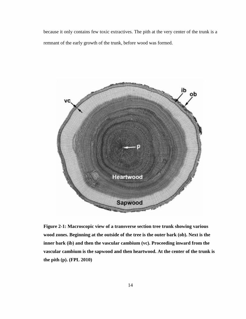
Figure 2-1: Macroscopic view of a transverse section tree trunk showing various wood

zones. Beginning at the outside of the tree is the outer bark (ob). Next is the inner

bark (ib) and then the vascular cambium (vc). Proceeding inward from the

vascular cambium is the sapwood and then heartwood. At the center of the trunk

is the pith (p). (FPL 2010)…………………..........................................................14

Figure 2-2: Cross section, tangential, and radial surfaces of a tree trunk………………..19

Figure 2-3: Light microscopic view, at left, of the lumina (L) and cell walls (arrowheads)

of a softwood. The right image represents hand-lens view of growth rings, each

composed of earlywood (ew) and latewood (lw). The light spots present in the

latewood are resin canals…………………………………………………….......20

Figure 2-4: Cut-away drawing of a cluster of cells, including structural details of a

bordered pit. In the middle cell, the various layers of the cell wall are detailed at

the top of the drawing, beginning with the middle lamella (ML). The next layer is

the primary wall (P), and on the surface of this layer the random orientation of the

cellulose microfibrils is detailed. Interior to the primary wall is the secondary wall

in its three layers: S1, S2, and S3. The mirofibril angle of each layer is illustrated,

as well as the relative thickness of the layers. The lower portion of the illustration

shows bordered pits in both sectional and face view. (FPL 2010)………………23

Figure 3-1: Photograph of the unilateral magnet device employed in this study. The white

circle on the face of the magnet array is the RF probe. The sensor is connected to

the Bruker Minispec console and the RF probe is placed adjacent to the wood

sample for moisture content measurements……………………………………...53

xi

Figure 3-2: Magnetic field along the central vertical line of the magnet array. The center

of the homogeneous spot is 1.3 cm from the surface of the magnet. This permits

measurement of signal within a finite volume inside the sample and not just on the

surface. In the case of wood logs, measurements of MR signal in the sapwood are

therefore possible without first removing the bark………………………………54

Figure 3-3: Time-domain bulk free induction decays (FIDs) signal as the black spruce

sapwood sample thaws from 0.15 h to 6.20 h employing the Nalorac 2.4 Tesla

horizontal bore superconducting magnet. The time between points on the FID was

5 µs. No short lifetime signal component was observed. The 𝑇2∗ increases from

330 µs to 1.2 ms. The signal amplitude increased by a factor of 3.1 as the sample

temperature changed from -20°C to 10°C………………………………………57

Figure 3-4: SPRITE MRI images of a black spruce sapwood sample in the transverse

(left) and tangential (right) planes as a function of thawing time at ambient

temperature. A moving ring boundary of thawing front was observed………….59

Figure 3-5: Displacement of the ring boundary of the thawing front both along and across

the grain directions from Figure 3-4, as a function of the square root of thawing

time. Displacement increases non-linearly as the black spruce sapwood sample

thaws. The thawing front progression is nearly identical both along and across the

grain……………………………………………………………………………...60

Figure 3-6: The one dimensional profiles (b and c) extracted from the transverse image in

Figure 3-4 at the positions indicated by the white lines (a). The signal intensity in

xii

the frozen sapwood region is similar to that in the unfrozen heartwood (bottom

region of the image (a))…………………………………………………………..62

Figure 3-7: Bi-exponential CPMG decay plots of signal intensity of samples thawed to

various extents. A unilateral magnet utilizing CPMG measurements was

employed. The initial sample temperature was -20°C and the surrounding

temperature was 3°C. At thawing time of: (a) 6 min, no phase transition of water

occurred; (b) 295 min, phase transition of the long lifetime signal component (free

water) was observed; (c) 345 min; and (d) 405 min. The quantity of free water

increased as more liquid water was created as a result from the sample thawing.64

Figure 3-8: Semi log plot of the signal intensity of the long lifetime components (free

water) of Figure 3-7 as a function of thawing time of black spruce sapwood. The

ring boundary of thawing emerges in the sensitive volume commencing at 200

minutes…………………………………………………………………………...66

Figure 3-9: Time-domain bulk free induction decays (FIDs) signal as the black spruce

heartwood sample thawed from 0.23 h to 4.60 h employing the Nalorac 2.4 Tesla

horizontal bore superconducting magnet. The 𝑻𝟐∗ signal lifetime was constant at

400 µs. No water phase transition was observed………………………………...67

Figure 3-10: SPRITE MRI images of a black spruce heartwood sample in the transverse

(left) and tangential (right) planes as a function of thawing time. No changes were

observed even after 4.6 hours of warming. The heartwood sample was at the fiber

saturation point, therefore, most of the water was in the cell walls. Bound water

was not frozen at measurement conditions………………………………………68

xiii

Figure 3-11: Time-domain bulk free induction decays (FIDs) as a function of time for

different temperatures as the black spruce sapwood sample froze. Signal

decreases with temperature as water underwent a phase change. The time between

points on the FID was 5 µs………………………………………………………69

Figure 3-12: Bulk MR signal intensity versus temperature as the black spruce sapwood

sample freezes: original data (●) and corrected (▽) for temperature as defined by

Curie’s Law. CPMG measurement was undertaken. An abrupt phase change of

free water occurred at -3°C. A second phase change (bound water) was observed

below -60°C……………………………………………………………………...71

Figure 3-13: Bulk signal intensity of bound (●) and free (o) water versus temperature

from the corrected data of Figure 3-12 as the black spruce sapwood sample froze.

CPMG measurement was undertaken. The ratio of signal from free and bound

water was approximately 3:1…………………………………………………….72

Figure 3-14: Bulk T2 of bound (●) and free (o) water versus temperature from the

corrected data of Figure 3-12 as the black spruce sapwood sample froze. CPMG

measurement was undertaken. The T2 of bound water was much shorter than the

T2 of free water…………………………………………………………………..74

Figure 3-15: 2D Spiral SPRITE images of a black spruce sapwood sample (2 mm x 25

mm x 25 mm). Each image is 64x64 pixels. High signal intensity corresponds to

high concentration of liquid water. Phase transition of free water occurred at -3oC.

A nonzero signal from -5oC to -60

oC suggests that bound water was not frozen at

these temperatures. Prior to the freezing phase transition of free water, the signal

of the earlywood was twice the signal of the latewood in a growth ring………...76

xiv

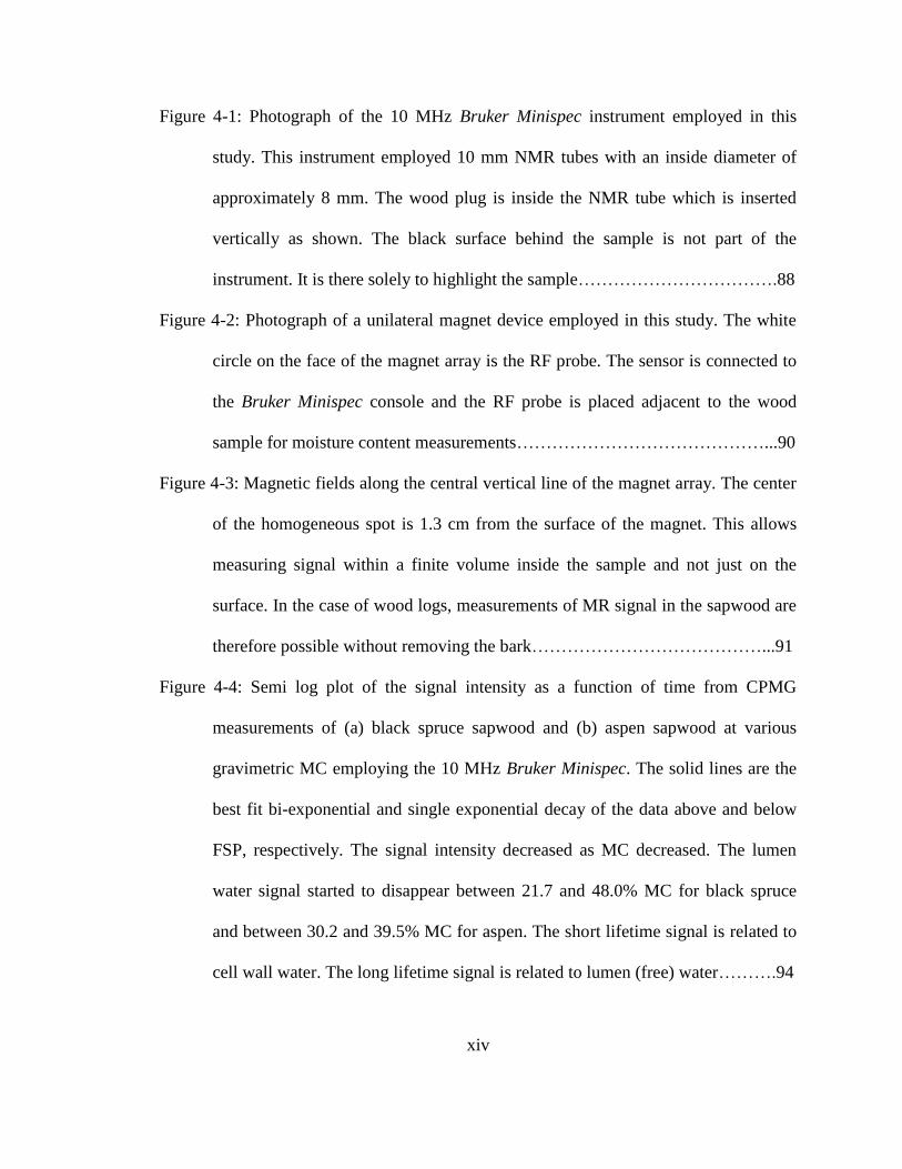
Figure 4-1: Photograph of the 10 MHz Bruker Minispec instrument employed in this

study. This instrument employed 10 mm NMR tubes with an inside diameter of

approximately 8 mm. The wood plug is inside the NMR tube which is inserted

vertically as shown. The black surface behind the sample is not part of the

instrument. It is there solely to highlight the sample…………………………….88

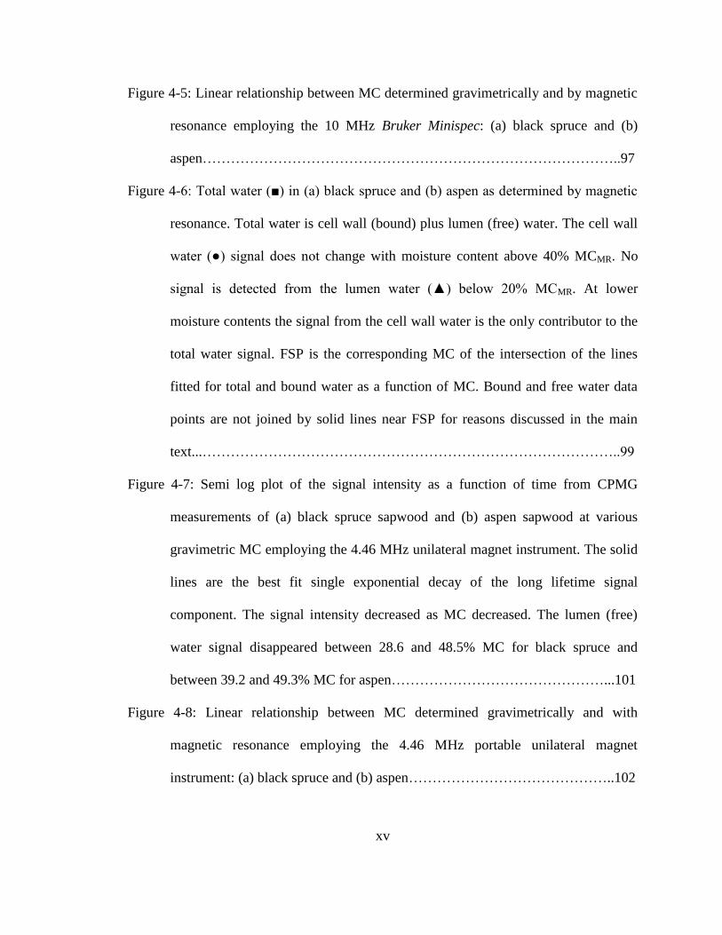
Figure 4-2: Photograph of a unilateral magnet device employed in this study. The white



sample for moisture content measurements……………………………………...90

Figure 4-3: Magnetic fields along the central vertical line of the magnet array. The center

of the homogeneous spot is 1.3 cm from the surface of the magnet. This allows

measuring signal within a finite volume inside the sample and not just on the


therefore possible without removing the bark…………………………………...91

Figure 4-4: Semi log plot of the signal intensity as a function of time from CPMG

measurements of (a) black spruce sapwood and (b) aspen sapwood at various

gravimetric MC employing the 10 MHz Bruker Minispec. The solid lines are the

best fit bi-exponential and single exponential decay of the data above and below

FSP, respectively. The signal intensity decreased as MC decreased. The lumen

water signal started to disappear between 21.7 and 48.0% MC for black spruce

and between 30.2 and 39.5% MC for aspen. The short lifetime signal is related to

cell wall water. The long lifetime signal is related to lumen (free) water……….94

xv

Figure 4-5: Linear relationship between MC determined gravimetrically and by magnetic

resonance employing the 10 MHz Bruker Minispec: (a) black spruce and (b)

aspen……………………………………………………………………………..97

Figure 4-6: Total water (■) in (a) black spruce and (b) aspen as determined by magnetic

resonance. Total water is cell wall (bound) plus lumen (free) water. The cell wall

water (●) signal does not change with moisture content above 40% MCMR. No

signal is detected from the lumen water (▲) below 20% MCMR. At lower

moisture contents the signal from the cell wall water is the only contributor to the

total water signal. FSP is the corresponding MC of the intersection of the lines

fitted for total and bound water as a function of MC. Bound and free water data

points are not joined by solid lines near FSP for reasons discussed in the main

text...……………………………………………………………………………..99



gravimetric MC employing the 4.46 MHz unilateral magnet instrument. The solid

lines are the best fit single exponential decay of the long lifetime signal

component. The signal intensity decreased as MC decreased. The lumen (free)

water signal disappeared between 28.6 and 48.5% MC for black spruce and

between 39.2 and 49.3% MC for aspen………………………………………...101

Figure 4-8: Linear relationship between MC determined gravimetrically and with

magnetic resonance employing the 4.46 MHz portable unilateral magnet

instrument: (a) black spruce and (b) aspen……………………………………..102

xvi

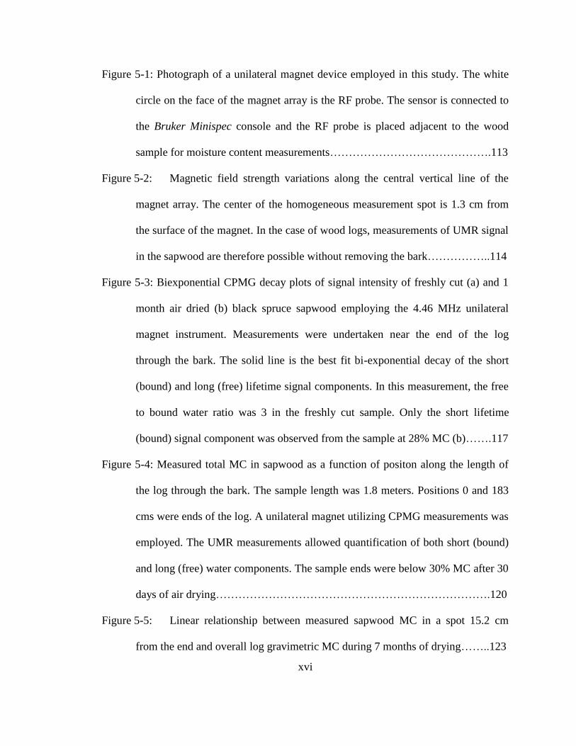
Figure 5-1: Photograph of a unilateral magnet device employed in this study. The white



sample for moisture content measurements…………………………………….113

Figure 5-2: Magnetic field strength variations along the central vertical line of the

magnet array. The center of the homogeneous measurement spot is 1.3 cm from

the surface of the magnet. In the case of wood logs, measurements of UMR signal

in the sapwood are therefore possible without removing the bark……………..114

Figure 5-3: Biexponential CPMG decay plots of signal intensity of freshly cut (a) and 1

month air dried (b) black spruce sapwood employing the 4.46 MHz unilateral

magnet instrument. Measurements were undertaken near the end of the log

through the bark. The solid line is the best fit bi-exponential decay of the short

(bound) and long (free) lifetime signal components. In this measurement, the free

to bound water ratio was 3 in the freshly cut sample. Only the short lifetime

(bound) signal component was observed from the sample at 28% MC (b)…….117

Figure 5-4: Measured total MC in sapwood as a function of positon along the length of

the log through the bark. The sample length was 1.8 meters. Positions 0 and 183

cms were ends of the log. A unilateral magnet utilizing CPMG measurements was

employed. The UMR measurements allowed quantification of both short (bound)

and long (free) water components. The sample ends were below 30% MC after 30

days of air drying……………………………………………………………….120

Figure 5-5: Linear relationship between measured sapwood MC in a spot 15.2 cm

from the end and overall log gravimetric MC during 7 months of drying……..123

xvii

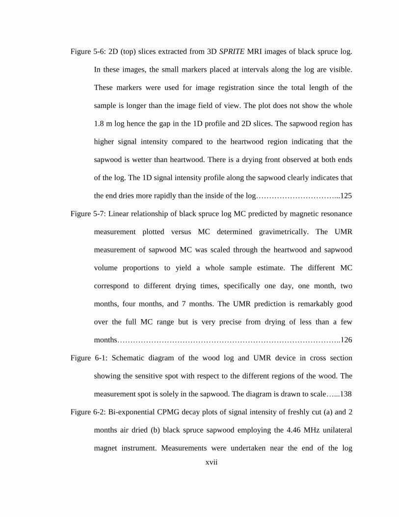
Figure 5-6: 2D (top) slices extracted from 3D SPRITE MRI images of black spruce log.

In these images, the small markers placed at intervals along the log are visible.

These markers were used for image registration since the total length of the

sample is longer than the image field of view. The plot does not show the whole

1.8 m log hence the gap in the 1D profile and 2D slices. The sapwood region has

higher signal intensity compared to the heartwood region indicating that the

sapwood is wetter than heartwood. There is a drying front observed at both ends

of the log. The 1D signal intensity profile along the sapwood clearly indicates that

the end dries more rapidly than the inside of the log…………………………...125

Figure 5-7: Linear relationship of black spruce log MC predicted by magnetic resonance

measurement plotted versus MC determined gravimetrically. The UMR

measurement of sapwood MC was scaled through the heartwood and sapwood

volume proportions to yield a whole sample estimate. The different MC

correspond to different drying times, specifically one day, one month, two

months, four months, and 7 months. The UMR prediction is remarkably good

over the full MC range but is very precise from drying of less than a few

months…………………………………………………………………………..126

Figure 6-1: Schematic diagram of the wood log and UMR device in cross section

showing the sensitive spot with respect to the different regions of the wood. The

measurement spot is solely in the sapwood. The diagram is drawn to scale…...138

Figure 6-2: Bi-exponential CPMG decay plots of signal intensity of freshly cut (a) and 2

months air dried (b) black spruce sapwood employing the 4.46 MHz unilateral

magnet instrument. Measurements were undertaken near the end of the log

xviii

through the bark. The solid line is the best fit bi-exponential decay of the short

(cell wall) and long (lumen) lifetime signal components. In this measurement, the

lumen to cell wall water ratio was 3 in the freshly cut sample (a). Only the short

lifetime signal component was observed from the sample at 15.2% MC (b)…..142

Figure 6-3: Measured total MC in sapwood as a function of positon along the length of

the log through the bark. A unilateral magnet utilizing CPMG measurements was

employed. The UMR measurements allowed quantification of both short and long

T2 water lifetime components. The sample ends were below 40% MC after 1

month of air drying……………………………………………………………..144

Figure 6-4: Total water (∆) in black spruce sapwood as determined by magnetic

resonance as a function of sample length. Total water is cell wall water plus

lumen water. Signal from cell wall water (●) does not change with moisture

content above 30% MC. No signal is detected from the lumen water (o) at both

ends of the log after 2 months of air drying. (a), (b), (c) and (d) correspond to 1

day, 1 week, 1 month and 2 months air drying duration, respectively. No

significant change in MC in the cell wall was observed until MC was below

FSP……………………………………………………………………………...146

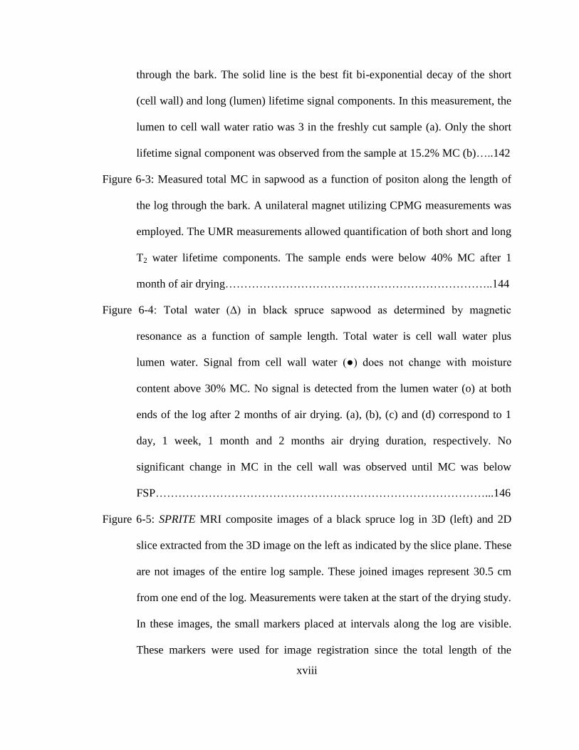
Figure 6-5: SPRITE MRI composite images of a black spruce log in 3D (left) and 2D

slice extracted from the 3D image on the left as indicated by the slice plane. These

are not images of the entire log sample. These joined images represent 30.5 cm

from one end of the log. Measurements were taken at the start of the drying study.

In these images, the small markers placed at intervals along the log are visible.

These markers were used for image registration since the total length of the

xix

sample is longer than the image field of view. The sapwood region has higher

signal intensity compared to the heartwood region indicating that the sapwood has

high MC…………………………………………………………………...........148

Figure 6-6: MC in sapwood (a) and heartwood (b) as a function of position along the

length of the log. Positions 0 and 91 cms correspond to the end and midpoint

along the length, respectively. These 1D profiles were extracted from the 3D

SPRITE MRI images. A decrease in MC was observed with increased drying

duration. Diffusive drying was observed at the end of the sample……………..150

Figure 6-7: SPRITE MRI images of black spruce log in the transverse plane (left) and

radial profiles (right) extracted vertically at the center of the composite image, as

a function of position along the length of the log. These data were taken after one

month of air drying. The sapwood region has higher signal intensity compared to

the heartwood region indicating that the sapwood has high MC. There is a drying

front observed near the end of the log. The MC in the sapwood and heartwood

regions near the end is less than the MCs in regions displaced from the end......151

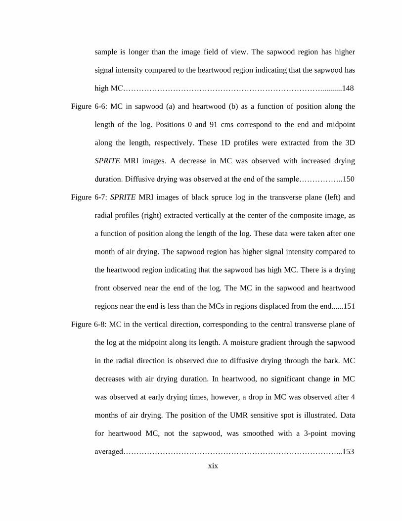
Figure 6-8: MC in the vertical direction, corresponding to the central transverse plane of

the log at the midpoint along its length. A moisture gradient through the sapwood

in the radial direction is observed due to diffusive drying through the bark. MC

decreases with air drying duration. In heartwood, no significant change in MC

was observed at early drying times, however, a drop in MC was observed after 4

months of air drying. The position of the UMR sensitive spot is illustrated. Data

for heartwood MC, not the sapwood, was smoothed with a 3-point moving

averaged………………………………………………………………………...153

xx

Figure 7-1: Magnetic field along the central vertical line of the magnet array. The center

of the homogeneous spot is 1.3 cm from the surface of the magnet. This permits

measurement of signal within a finite volume inside the sample and not just on the


therefore possible without first removing the bark……………………………..165

Figure 7-2: Photos of the field measurements: (a) markings at the end of the log for

consistent orientation; (b) UMR measurements at the midpoint longitudinally..168

Figure 7-3: Average daily temperature and relative humidity near the drying stack......169

Figure 7-4: Total water signal in black spruce sapwood in a measurement spot 15 cm

from the end of the log, as determined by UMR. The sub-figures a-f are for each

of the 6 logs. The standard deviation of 4 measurements is illustrated with the

error bars………………………………………………………………………..172

Figure 7-5: Total water signal in black spruce sapwood at the midpoint longitudinally, as

determined by UMR……………………………………………………………174

Figure 7-6: Linear relationship between sapwood MC in a spot 15 cm from the end (a)

and at the midpoint longitudinally (b) to that of the overall log gravimetric MC in

the case of Log 3………………………………………………………………..176

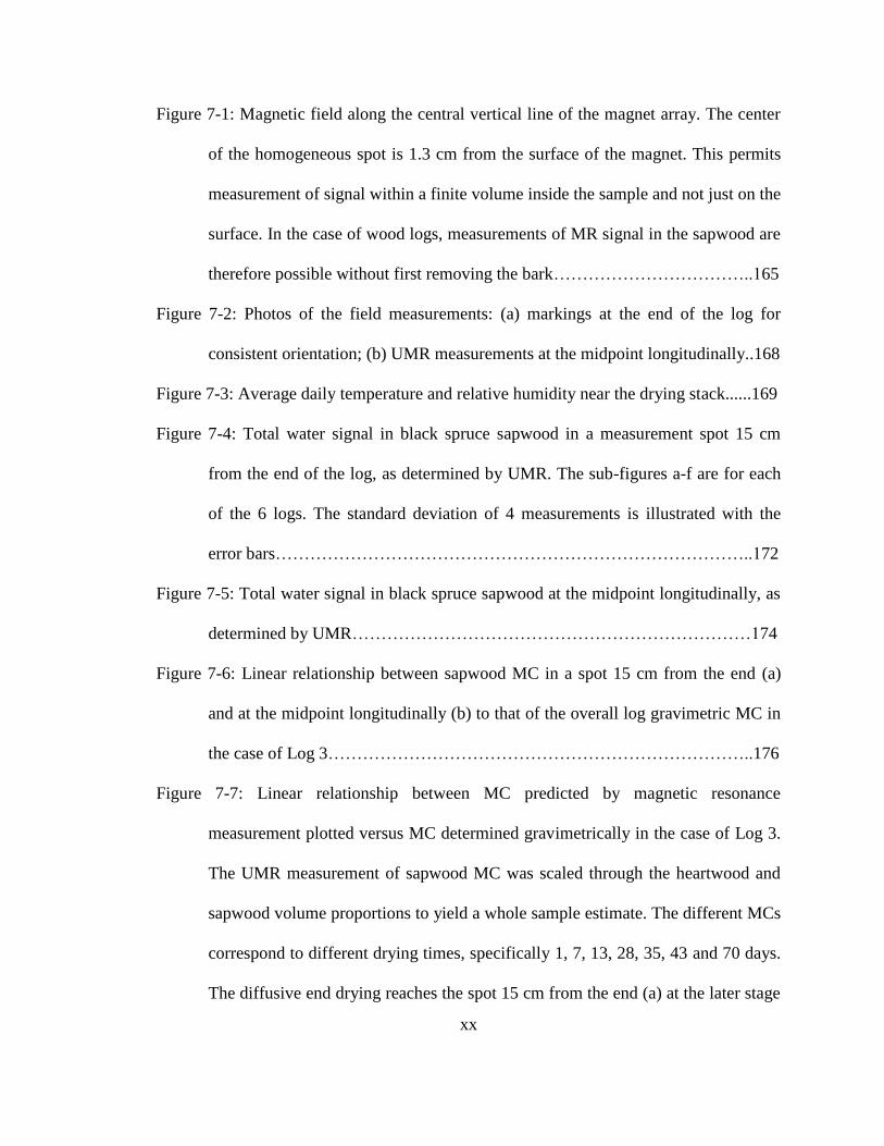
Figure 7-7: Linear relationship between MC predicted by magnetic resonance

measurement plotted versus MC determined gravimetrically in the case of Log 3.

The UMR measurement of sapwood MC was scaled through the heartwood and

sapwood volume proportions to yield a whole sample estimate. The different MCs

correspond to different drying times, specifically 1, 7, 13, 28, 35, 43 and 70 days.

The diffusive end drying reaches the spot 15 cm from the end (a) at the later stage

xxi

of drying. The better location when accessible is at the midpoint longitudinally

(b)……………………………………………………………………………….180

xxii

List of Symbols, Nomenclature or Abbreviations

1D One-dimensional

2D Two-dimensional

3D Three-dimensional

a.u. Arbitrary units

α Radio frequency flip angle

γ Gyromagnetic ratio (42.58 MHz/Tesla in the case of 1H)

B0 Magnetic field strength

M0 Net magnetization

N Number of 1H nuclei

T Temperature

I Spin quantum number

h Planck’s constant

ħ h/2π

kB Boltzmann’s constant

𝜔 Resonance frequency also known as the Larmor frequency

D2O Deuterium oxide

DSC Differential scanning calorimetry

ew Earlywood

FSP Fiber saturation point

GPR Ground penetrating radar

ib Inner bark

L Lumina

xxiii

lw Latewood

kg kilogram

MC Moisture content

MClog Overall MC of the log

MCheartwood MC of heartwood

MCsapwood MC of sapwood

Mg Mass of the moist (green) wood sample

Mod Mass of the oven-dry wood sample

MR Magnetic resonance

MRI Magnetic resonance imaging

ms millisecond

NIR Near-infrared

NMR Nuclear magnetic resonance

ob Outer bark

p Pith

RF Radio frequency

SNR Signal to noise ratio

SPRITE Single Point Ramped Imaging with T1 Enhancement

S Signal intensity

S0 Signal intensity at time = 0

TE Echo time

TIR Thermal infrared

tp Phase encode time

xxiv

T1 Spin-lattice relaxation time

T2 Spin-spin relaxation time

𝑇2∗ Effective spin-spin relaxation time constant

UM Unilateral magnet

UMR Unilateral magnetic resonance

CPMG Carr-Purcell-Meiboom-Gill

VIS Visible

Volheartwood Volume of heartwood

Volsapwood Volume of sapwood

vc Vascular cambium

1

Chapter 1 – Introduction

1.1 Overview

In Canada, forestry and forest products are vital to the health, wealth and growth

of the economy. In 2012, Canada's forest products industry was a 57 billion dollar a year

industry that represented 12% of the country’s manufacturing Gross Domestic Product

(Forest Products Association of Canada 2012). In 2013, the Canadian forest industry

achieved a profit of C$2.7 billion, the highest profit in the last 8 years (Natural Resources

Canada 2015). However, the Canadian forest industry is in turmoil due to high

production costs that make it difficult to compete with other countries; low cost

producers and fast fiber growers. To stay competitive and reduce production costs, the

industry must continue to innovate. In particular, it needs to use fast and reliable

analytical techniques to improve product quality and optimize processes. Innovation and

process optimization are important in numerous stages of the forest products industry.

These include harvesting, resource management, pulp and fiber yield assessment, scaling

and grading of wood products.

One of the most important properties to be monitored in any wood process is

moisture content (MC). Currently, MC is poorly monitored due to the absence of reliable

and rapid methods which measure water directly. An ideal method should have direct

detection of water and thus gives a linear response with MC, ie., double the amount of

MC equals double the signal. The ideal method should also be non-destructive and rapid.

The most common and widely accepted standard in MC measurement is the

gravimetric method (ASTM Standard D4442-07). This method is destructive and time

2

consuming. Furthermore, there is a practical limitation to the size of wood sample that

can be used. For chemically treated wood or wood species with high volatile extractive

contents, the distillation method of determining MC is recommended (ASTM Standard

D4442-07). However, like the gravimetric method, this technique is time consuming and

destructive. Alternative methods, often based on sensors, have been developed in order to

address these limitations.

Electric moisture meters for wood measure electric conductance (resistance) or

dielectric properties, which vary with MC when MC is less than 30% (James 1988).

Conductance (resistance) type meters use penetrating electrodes that are pushed into the

wood, and thus can be considered destructive in some wood product applications.

Dielectric meters use surface electrodes that do not puncture the wood surface, and can

measure the MC of relatively dry wood. Electric moisture meters are species dependent

and do not have a linear response to MC particularly at high MC.

There are numerous non-destructive techniques available for measuring wood

MC (Bucur 2003). These techniques include methods based on X-ray and gamma rays,

near-infrared (NIR), microwaves, terahertz (THz), acoustic waves, and magnetic

resonance (MR).

X-ray and gamma ray sensors employ ionizing radiation and require highly

trained personnel in order to properly use the instruments. X-rays have been utilized for

wood density measurements, for wood moisture monitoring, and for observing internal

log features that include pith, sapwood, heartwood, knots, and other defects (So et al.

2004, Wei et al. 2011). However, X-ray measurements were demonstrated to be related to

both density and MC measurements in the same image. That is why X-ray methods in

3

wood MC measurements require two x-ray images, with the sample wet and then oven-

dried. In many cases, it is impractical to oven-dry samples like timber or a living tree to

determine its MC. Recent developments in X-ray technology, in particular the principle

of dual-energy x-ray absorptiometry, has the potential to address this issue (Kullenberg et

al. 2010, Tanaka and Kawai 2013, Kim et al. 2015).

There are commercial systems (handheld and imaging) that employ NIR radiation

to measure solid wood (Leblon et al 2013). Similar to X-ray, NIR radiation is not

selective for MC, it is also sensitive to wood density. In addition, its penetration depth in

solid wood is limited, ranging from 1 to 5 mm depending on surface roughness and the

wavelength employed (Tsuchikawa et al. 1996). A NIR handheld spectroradiometer has

been employed to determine MC and basic density of thawed and frozen logs (Hans et al.

2013 and 2015a). Similarly hyperspectral images were employed to map moisture content

and basic density in thawed and frozen board and logs (Haddadi et al. 2015a, 2015b and

2016).

Commercial microwave moisture meters have been employed for wood MC

measurements, however, microwave adsorption is not solely dependent on MC. It also

depends on wood density (Trabelsi and So 1998). Proper calibration of microwave

moisture meters is of great importance to address errors associated with material density

and its effect on MC measurement. Manufacturers have developed density-independent

microwave moisture meters (Kraszewski 1973, Meyer 1981, Trabelsi and So 1997).

More recently ground penetration radar (GPR), which also uses microwave

radiation, was evaluated for measurement of wood log MC (Hans et al 2015b and 2015c).

While GPR sensors can easily handle both frozen and thawed wood material, they have

4

some limitations with logs such as a poor surface-antenna coupling due to the rounded

shape of the logs (Redman et al.2016), and significant attenuation of the signal at high

frequencies (Nicolotti et al. 2003).

Terahertz spectroscopy and imaging are new and promising tools for MC

determination in wood materials. The THz radiation is intermediate in wavelength

between NIR and microwave radiation in the electromagnetic radiation spectrum. THz

spectroscopy and imaging have been employed in wood science research (Todoruk et al.

2012, Inagaki et al. 2014a, 2014b), for wood density mapping (Koch et al. 1998), wood

defect detection (Oyama et al. 2009), determining properties of paper (Mousavi et al.

2009) and imaging of wood MC (Teti et al. 2011). THz radiation penetration is limited,

ranging from surface to near subsurface (about 5 mm) in dry solid wood.

Ultrasonics can be employed to measure log MC, but only for liquid water, i.e., at

temperatures above the freezing point (Nader 2007). Furthermore, the relationship

between MC and acoustic parameters, due for example to sample density, was shown to

vary between species and within the same species (Nader 2007).

Ultrasonics can be employed to measure log MC, but only for liquid water, i.e., at

temperatures above the freezing point (Nader 2007). Furthermore, the relationship

between MC and acoustic parameters was shown to vary between species, and within the

same species, due for example to sample density (Nader 2007).

More details are given in Chapter 2 for the most common MC measurement

techniques, outlined above, employed in the forest products industry.

Magnetic resonance (MR) and magnetic resonance imaging (MRI) are well

known methodologies for molecular structure determination and medical imaging. In

5

each case, MR measures the quantity of hydrogen containing material in the sample of

interest, with secondary information on the molecular dynamics and molecular

environment. In the context of wood materials, MR and MRI offer the possibility of non-

invasive determination of cell wall and lumen water concentration in materials, spatially

resolved (Araujo 1993, Casieri et al. 2004, MacMillan et al. 2002).

This thesis investigates and evaluates the use of a portable unilateral magnetic

resonance (UMR) device, a benchtop MR instrument and MRI in monitoring and

quantifying water content in wood. Such measurements are necessary in the forest

products industry to optimize processes where reliable and accurate MC measurements

are required. Recently developed handheld UMR devices permit ‘spot’ measurements of

water content inside the material of interest (Marble et al. 2007). This approach permits a

small sensor, exterior to the sample, to survey, as required, a large sample. In

combination with the whole-sample laboratory MRI methods developed at UNB,

uniquely quantitative for water content, this thesis investigated laboratory and field

measurements of water content in wood log moisture estimation.

The majority of work undertaken in this thesis employed black spruce as the

wood material. Black spruce was suggested by,. FPInnovations, our sponsor and partner

in the Natural Science and Engineering Research Council of Canada Strategic Grant

which supported this thesis work. Black spruce is an important wood species in Eastern

Canada. Aside from pulpwood, this species is also used for lumber, construction plywood

and packaging/containers. Wood samples were supplied by FPInnovations through their

industry members.

6

1.2 Thesis organization

The organization of this thesis is outlined below.

Chapter 1 provides an introduction as well as an outline of the thesis work.

Chapter 2 discusses wood and the nature of water in wood. It considers, in

particular, the structure of wood and its composition. It also discusses the nature of water

in wood as the wood dries. This chapter provides basic information on the conventional

techniques employed by the forest industry in MC measurements. Basic background

information on MR is also discussed. Lastly, a review of MR work on water in wood is

provided.

Chapter 3 examines the phase transitions of water in wood by UMR and MRI.

The objective was to observe and understand the behavior of water below 0°C in wood.

The results show that for the species studied, black spruce (Picea mariana Mill.), one

abrupt phase change occurred around -3°C, which was attributed to the phase transition

of lumen water. A more diffuse change occurred below -60°C which was attributed to a

phase transition of cell wall water. UMR was demonstrated to be a powerful tool in the

study of water in wood. This chapter was based on a paper that has been published in

Wood and Fiber Science Journal (Lamason et al. 2014). This paper was awarded second

place in the 2015 George Marra award for excellence in writing and research, by the

Society of Wood Science and Technology, USA.

Chapter 4 discusses how time-domain MR measurements easily distinguish water

in different environments in wood according to the spin-spin relaxation time and provide

quantitative information on water content. A portable UMR device was employed to

measure water content in black spruce (Picea mariana Mill.) and aspen (Populus

7

tremuloides Michx.). A benchtop MR device which has a homogenous magnetic field

was employed to compare the results of the UMR device. This chapter was based on a

paper that has been published in Wood Material Science and Engineering (Lamason et al.

2015).

Chapter 5 is a laboratory study that shows how UMR permits one to estimate total

MC as a log dries when one measures MC in the sapwood, displaced from the log ends.

The goal was to determine the best location to make spot MC measurements in wood logs

to permit an estimate of the whole sample MC. The paper describing the work was

submitted to the European Wood Products Journal. The authors withdrew the submission

after waiting more than one year for review. Some of the major conclusions of the paper

reappeared in the work of Chapter 7.

Chapter 6 examines why the spot resolved black spruce sapwood measure of MC

gives good estimates of the whole log MC. The goal was to understand drying behaviors

of different regions in wood logs. This chapter provides spatially resolved measurement

(UMR and MRI) of MC as wood log dried. This paper has been published in the Forest

Products Journal (Lamason et al. 2016a).

Chapter 7 demonstrates in a field study, with multiple samples, that the UMR spot

measurement in black spruce sapwood, displaced from the drying end, is a good predictor

of overall log MC. This chapter was based on a paper that has been published in the

Forest Products Journal (Lamason et al. 2016b).

For Chapters 3 through 7, the author of the thesis designed the experimental

procedure with the assistance of his supervisors and advisory committee, performed all of

8

the experiments, data analysis, and wrote the corresponding articles of which he is first

author.

Chapter 8 provides the conclusions of this thesis and recommendations for future

work.

This thesis is written in the form of a thesis with chapters as papers. The content

has been structured such that successive topics build on one another and flow naturally

between successive chapters.

9

1.3 References

ASTM Standard D4442-07 (2007). Direct moisture content measurement of wood and

wood-base materials. ASTM International, West Conshohocken, PA. doi:

10.1520/D4442-07.

Araujo CD, MacKay AL, Hailey JRT, Whittall KP, and Le H (1992) Proton magnetic

resonance techniques for characterization of water in wood: application to white

spruce. Wood Sci Tech. 26 (2):101-113.

Bucur V. (2003) Nondestructive characterization and imaging of wood. Berlin

Heidelberg, Germany: Springer-Verlag. ISBN? PAGES?

Casieri C, Senni L, Romagnoli M, Santamaria U, and DeLuca F (2004) Determination of

moisture fraction in wood by mobile NMR device. J. Magn. Reson 171(2):364-

372.

Forest Products Association of Canada (2012) Industry by the numbers: Forest Products

Association of Canada. http://www.fpac.ca/index.php/en/industry-by-the-

numbers/

Haddadi A, Burger J, Leblon B, Pirouz Z, Groves K, Pirouz Z, and Nader J (2015a) Use

pf hyperspectral images over amabilis fir boards. Part 1: Moisture content

estimation. Wood Mat. Sci. Eng. 10(1):27-40.

Haddadi A, Burger J, Leblon B, Groves K, Pirouz Z, and Nader J (2015b) Use of

hyperspectral images over amabilis fir boards. Part 2: Density and basic specific

estimation, Wood Mat. Sci. Eng., 10(1):41-56.

Haddadi A, Leblon B, Pirouz Z, Groves K, and Nader J (2016) Use of hyperspectral

images for estimating moisture content and density of frozen and unfrozen logs.

Wood Sci. Tech., 50(2):221-243.

Hans G, Leblon B, LaRocque A, Stirling R, Nader J, Cooper P (2013) Monitoring

moisture content and basic specific gravity of black spruce logs using a handheld

MEMS-based near-infrared spectrometer. Forest Chronicle 89(5):607-620.

Hans G, Leblon B, LaRocque A, Stirling R, Nader J, Cooper P (2015a) Monitoring

moisture content and basic specific gravity of aspen and poplar logs using a

handheld MEMS-based near-infrared spectrometer. Wood Mat. Sci. Eng. 10(1):3-

16.

Hans G, Redman D, Leblon B, Nader J, and LaRocque A (2015b) Determination of log

moisture content using ground penetrating radar. Part 1. Partial least squares

(PLS) method. Holzforschung 69(9):1117-1123.

http://www.fpac.ca/index.php/en/industry-by-the-numbers/

http://www.fpac.ca/index.php/en/industry-by-the-numbers/

10

Hans G, Redman D, Leblon B, Nader J, and LaRocque A (2015c) Determination of log

moisture content using ground penetrating radar. Part 2. Propagation Velocity

(PV) method. Holzforschung 69(9):1125-1132.

Inagaki T, Ahmed B, Hartley ID, Tsuchikawa S, Reid M (2014a) Simultaneous

prediction of density and moisture content of wood by terahertz time domain

spectroscopy. J Infrared Milli Terahz Waves 35:949-961.

Inagaki T, Hartley ID, Tsuchikawa S, Reid M (2014b) Prediction of oven-dry density of

wood by time-domain terahertz spectroscopy. Holzforschung 68(1):61-68.

James WL (1988) Electrical moisture meters for wood. USDA, Forest Service, Forest

Products Laboratory, General Technical Report FPL GTR-6. PAGES?

Kim C-K, Oh J-K, Hong J-P, and Lee J-J (2015) Dual-energy x-ray absorptiometry with

digital radiograph for evaluating moisture content of green wood. Wood Sci Tech.

49:713-723.

Koch M, Hunsche S, Schuacher P, Nuss MC, Feldman J, and Fromm J (1998) THz-

imaging: a new method for density mapping of wood. Wood Sci Tech. 32:421-

427.

Kraszewskit A (1973) Microwave instrumentation for moisture content measurement. J

Microwave Power 8(3/4):323-335.

Kullenberg R, Hultnäs M, Fernandez V, Nylinder M, Toft S, and Danielson F (2010)

Dual-energy X-ray absorptiometry analysis for the determination of moisture

content in biomass. J. Biobased Mat. Bioenergy 4:363-366.

Lamason C, MacMillan B, Balcom BJ, Leblon B, Pirouz Z (2014) Examination of water

phase transitions in black spruce by magnetic resonance and magnetic resonance

imaging. Wood Fiber Sci 46(4):1-14. (also Chapter 3 of this Thesis)

Lamason C, MacMillan B, Balcom BJ, Leblon B, Pirouz Z (2015) Water content

measurement in black spruce and aspen sapwood with bencthtop and portable

magnetic resonance devices. Wood Mat. Sci. Eng.10(1):86-93. (also Chapter 4 of

this Thesis)

Lamason C, MacMillan B, Balcom BJ, Leblon B, Pirouz Z (2016a) Magnetic resonance

studies of wood log-drying processes. Forest Products J. (doi: 10.13073/FPJ-D-

16-00037). (also Chapter 6 of this Thesis)

Lamason C, MacMillan B, Balcom BJ, Leblon B, Pirouz Z (2016b) Field measurements

of moisture content in black spruce logs with unilateral magnetic resonance.

11

Forest Products J. (doi: 10.13073/FPJ-D-16-00004). (also Chapter 7 of this

Thesis)

Leblon B, Adedipe O, Hans G, Haddadi A, Tsuchikawa S, Burger J, Stirling R,

LaRocque A, Pirouz Z, Groves K, Nader J (2013) A review of near infrared

spectroscopy for monitoring wood moisture content and bulk density, Forestry

Chronicle, 89(5):595-606.

MacMillan B, Schneider MH, Sharp AR, and Balcom BJ (2002) Magnetic resonance

imaging of water concentration in low moisture content wood. Wood Fiber Sci.

2:276-286.

Marble AE, Mastikhin IV, Colpitts BG, and Balcom BJ (2007) A compact permanent

magnet array with a remote homogenous field. J. Magn. Reson. 186(1):100-104.

Meyer W, Schilz W (1981) Feasibility study of density-independent moisture

measurement with microwaves. IEEE Transactions on microwave theory and

techniques, Vol. MIT-29 (7):732-739.

Mousavi P, Haran F, Jez D, Santosa F, Dodge JS (2009) Simultaneous composition and

thickness measurement of paper using terahertz time-domain spectroscopy. Appl.

Optics 48:6541-6546.

Nader J (2007) Evaluation of two technologies to determine the moisture content of logs.

FPInnovations, Pointe-Claire, QC, Canada, pp. 14.

Natural Resources Canada (2015) The state of Canada’s forests: Annual report 2014,

Canadian Forest Service, Government of Canada, Fo1-6/2014E, 63 pages.

Nicolotti G, Socco LV, Martinis R, Godio A, and Sambuelli L (2003) Application and

comparison of three tomographic techniques for detection of decay in trees. J.

Arboriculture 29:66-78.

Oyama Y, Zhen L, Tanabe T, and Kagaya M (2009) Sub-terahertz imaging of defects in

building blocks. NDT&E Int. 42:28-33.

Redman, D., Hans, G., & Diamanti, N. (2016) Impact of wood sample shape and size on

moisture content measurement using a GPR based sensor. IEEE J. Sel. Topics

Appl Earth Obs. Remote Sens. 9(1):221-227.

So CL, Via BK, Groom LH, Schimleck LR, Shupe TF, Kelley SS, and Rials TG (2004)

Near-infrared spectroscopy in the forest products industry. Forest Products J.

53(3):6-16.

12

Tanaka T, and Kawai Y (2013) A new method for non-destructive evaluation of solid

wood moisture content based on dual-energy X-ray absorptiometry. Wood Sci.

Tech. 47:1213-1229.

Teti A, Rodriguez D, Federici J, Brisson C (2011) Non-destructive measurement of water

diffusion in natural cork enclosures using terahertz spectroscopy and imaging. J

Infrared Millim Terahz Waves 32:513-527.

Todoruk TM, Hartley ID, Reid ME (2012) Origin of birefringence in wood at terahertz

frequencies. IEEE Trans. Terahertz Sci. Technol. 2:123–130.

Trabelsi S, and Nelson SO (1998) Density-independent functions for on-line microwave

moisture meter: a general discussion. Meas Sci Technol 9:570-578.

Tsuchikawa S, Torii M, and Tsutsumi S (1996) Application of near-infrared

spectrophotometry to wood. 4. Calibration equations for moisture content. J.

Japan Wood Res. Soc. 42(8):743–754.

Wei Q, Leblon B, and LaRocque A (2011) On the use of X-ray computed tomography for

determining wood properties: a review. Can. J. Forest Res. 41:2120-2140.

13

Chapter 2 – Wood and Water in Wood

2.1 Structure of wood

Trees are divided into two categories: Hardwoods and softwoods, based on their

seed characteristics. Softwoods have needle like leaves and are commonly called

evergreens. The seeds of softwoods are basically unprotected, usually inside scaly cones,

and are therefore often referred to as conifers. Hardwoods have broad leaves, which

generally change color and drop in the autumn in temperate zones: Hardwoods produce

seeds within acorns, pods or other fruiting bodies. The wood formed by softwoods and

hardwoods contain different types of cells. Hardwoods are not necessarily more dense or

harder than softwood, as their names imply (Haygreen and Bowyer 1982).

Figure 2-1 shows a cross sectional slice of a hardwood log. A cross sectional slice

of a softwood log is similar, except that often the growth rings are more distinct. Cell

division occurs in an outer layer called the cambium. The cells become part of the bark

(phloem) or part of the wood (xylem). Phloem (inner bark) is the principal tissue

concerned with the distribution of elaborated foodstuffs, characterized by the presence of

sieve tubes. The newer cells in the xylem are referred to as sapwood, and in a freshly cut

or green sample these cells are filled with water. Sapwood is defined as the portion of the

wood that in the living tree contains living cells and reserve materials such as starch

(IAWA 1964). It contains the wood that is part of the transpiration stream of the tree, and

generally has a high MC. Its permeability is facilitated by the presence of unaspirated,

unencrusted pits. Once cut (dead wood), sapwood becomes more susceptible to decay

14

because it only contains few toxic extractives. The pith at the very center of the trunk is a

remnant of the early growth of the trunk, before wood was formed.

Figure 2-1: Macroscopic view of a transverse section tree trunk showing various

wood zones. Beginning at the outside of the tree is the outer bark (ob). Next is the

inner bark (ib) and then the vascular cambium (vc). Proceeding inward from the

vascular cambium is the sapwood and then heartwood. At the center of the trunk is

the pith (p). (FPL 2010)

15

Heartwood is defined as the inner layers of the wood, which, in the growing tree

have ceased to contain living cells, and in which the reserve materials (e.g. starch) have

been removed and converted into heartwood substance. In general, cells in the heartwood

have lower MC, especially in softwood, and are usually high in extractives, which are

produced from starches and sugars giving fats, waxes, oils, resins, gums, tannin, and

aromatic and colouring materials (Haygreen and Bowyer 1982). In some species,

heartwood may be distinguished from sapwood by a darker color, lower permeability,

and increased decay resistance.

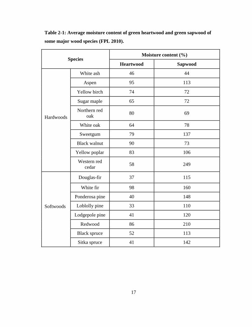
The average MC of green heartwood and green sapwood of some major North

American wood species is given in Table 2-1. These values are considered typical, but

variation within and between species is considerable (FPL 2010).

The sapwood is the region responsible for conducting water and minerals, and the

heartwood gives the tree mechanical support (Gartner 1995). Sufficient sapwood is

required to supply the foliage with water, and the amount of foliage on a tree is often

strongly correlated to the amount of sapwood (Berthier et al. 2001, Ryan 1989). When

individual growth increments of temperate-zone woods are examined, it is generally

apparent that the portion formed in the early part of the growing season has larger cells

and is lower in density than that formed later in the season; this part of the increment is

called the earlywood and is also known as springwood. The denser and usually darker-

colored wood formed in the last part of the growing season is called latewood or

summerwood (Panshin and de Zeeuw 1980).

A juvenile region, the first 5-20 central growth rings, contains shorter cells and

has fewer latewood cells than mature wood cells, although there is no abrupt division to

16

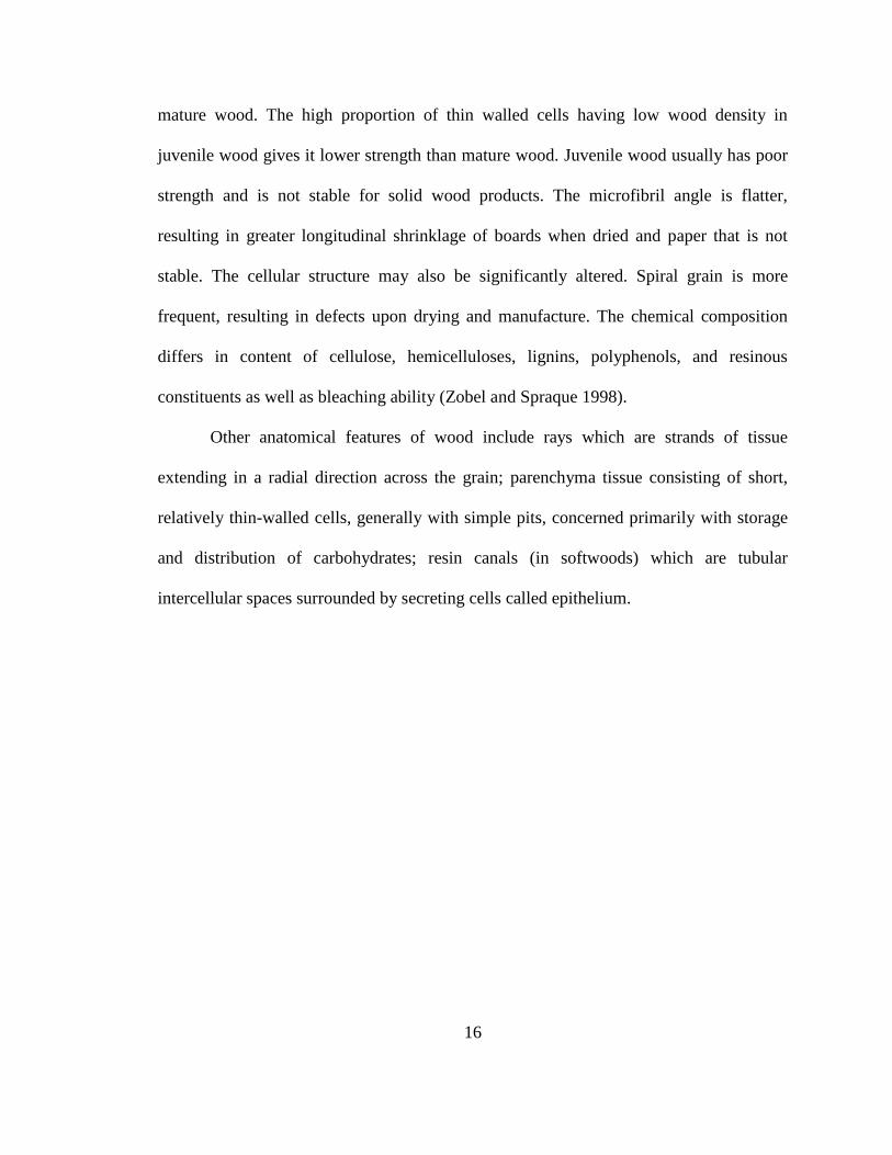
mature wood. The high proportion of thin walled cells having low wood density in

juvenile wood gives it lower strength than mature wood. Juvenile wood usually has poor

strength and is not stable for solid wood products. The microfibril angle is flatter,

resulting in greater longitudinal shrinklage of boards when dried and paper that is not

stable. The cellular structure may also be significantly altered. Spiral grain is more

frequent, resulting in defects upon drying and manufacture. The chemical composition

differs in content of cellulose, hemicelluloses, lignins, polyphenols, and resinous

constituents as well as bleaching ability (Zobel and Spraque 1998).

Other anatomical features of wood include rays which are strands of tissue

extending in a radial direction across the grain; parenchyma tissue consisting of short,

relatively thin-walled cells, generally with simple pits, concerned primarily with storage

and distribution of carbohydrates; resin canals (in softwoods) which are tubular

intercellular spaces surrounded by secreting cells called epithelium.

17

Table 2-1: Average moisture content of green heartwood and green sapwood of

some major wood species (FPL 2010).

Species Moisture content (%)

Heartwood Sapwood

Hardwoods

White ash 46 44

Aspen 95 113

Yellow birch 74 72

Sugar maple 65 72

Northern red

oak 80 69

White oak 64 78

Sweetgum 79 137

Black walnut 90 73

Yellow poplar 83 106

Western red

cedar 58 249

Softwoods

Douglas-fir 37 115

White fir 98 160

Ponderosa pine 40 148

Loblolly pine 33 110

Lodgepole pine 41 120

Redwood 86 210

Black spruce 52 113

Sitka spruce 41 142

18

Reaction wood forms in both softwood and hardwoods. In softwood, reaction

wood forms on the bottom side of a leaning stems and branches and is called

compression wood. Compression wood cells are typically 30% shorter, have 10% less

cellulose and 8-9% more lignin and hemicellulose. Compression wood has a high

proportion of latewood and often forms wide growth rings so that growth is eccentric

about the pith. In hardwoods, reaction wood forms on the top side of leaning stems and

branches and is called tension wood. Tension wood has fewer and smaller vessels, fewer

ray cells, and thick walled, small lumen fibers. The secondary cell wall layer is almost

pure cellulose and loosely connected to the primary wall. Tension wood also has wide

growth rings so that growth is eccentric about the pith (Haygreen and Bowyer 1982).

Wood is a naturally anisotropic material. Its properties vary widely when

measured with or against the growth grain. In a tree, three sections can be defined as:

cross section or transversal, tangential, and radial (Figure 2-2).

19

Figure 2-2: Cross section, tangential, and radial surfaces of a tree trunk.

2.2 Cell wall composition and structure

Figure 2-3 shows cross section images of a softwood. Hardwoods differ from

softwoods in possessing vessel elements, which when viewed in the transverse section

are called pores, hence hardwoods are also referred to as porous wood. The fibers in

hardwoods function almost exclusively as mechanical supporting cells (FPL 2010).

Softwoods are said to be nonporous in the sense that they do not contain vessels. For

black spruce the diameter and length of longitudinal tracheid cells are approximately 35

µm and 3.25 mm, respectively (Panshin and de Zeeuw 1980). Note that lumen size varies

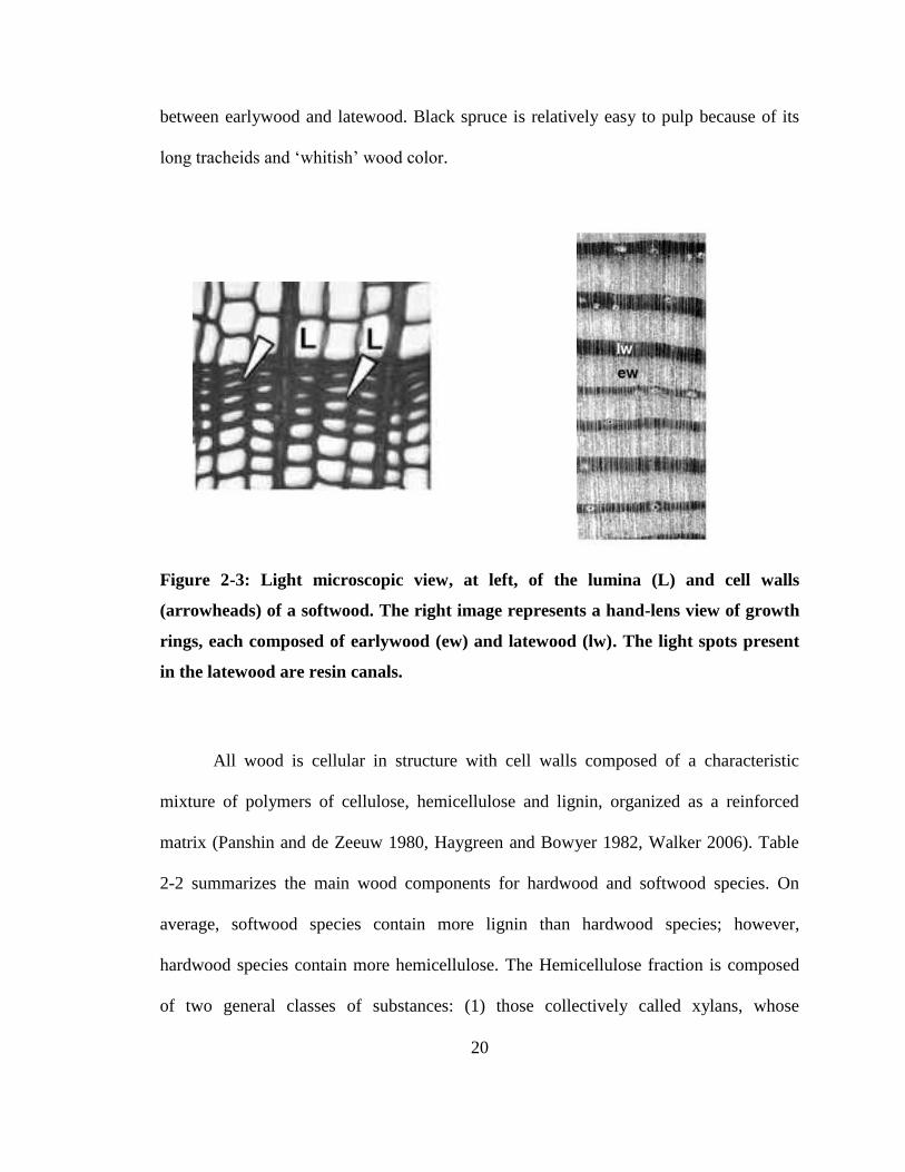
20

between earlywood and latewood. Black spruce is relatively easy to pulp because of its

long tracheids and ‘whitish’ wood color.

Figure 2-3: Light microscopic view, at left, of the lumina (L) and cell walls

(arrowheads) of a softwood. The right image represents a hand-lens view of growth

rings, each composed of earlywood (ew) and latewood (lw). The light spots present

in the latewood are resin canals.

All wood is cellular in structure with cell walls composed of a characteristic

mixture of polymers of cellulose, hemicellulose and lignin, organized as a reinforced

matrix (Panshin and de Zeeuw 1980, Haygreen and Bowyer 1982, Walker 2006). Table

2-2 summarizes the main wood components for hardwood and softwood species. On

average, softwood species contain more lignin than hardwood species; however,

hardwood species contain more hemicellulose. The Hemicellulose fraction is composed

of two general classes of substances: (1) those collectively called xylans, whose

21

molecules are formed by polymerization of the anhydro forms of xylose, arabinose, and

4-methylglucuronic acid, and (2) hemicelluloses called galactoglucose mannans, whose

molecules are formed by polymerization of residues of galactose, glucose, and mannose.

Xylans predominate in hardwoods and galactoglucomannans in softwoods (Panshin and

de Zeeuw 1980).

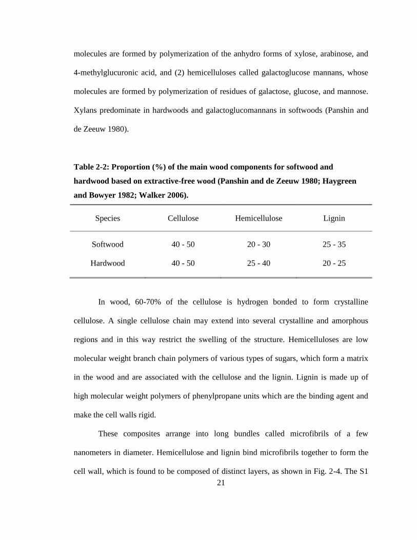
Table 2-2: Proportion (%) of the main wood components for softwood and

hardwood based on extractive-free wood (Panshin and de Zeeuw 1980; Haygreen

and Bowyer 1982; Walker 2006).

Species Cellulose Hemicellulose Lignin

Softwood 40 - 50 20 - 30 25 - 35

Hardwood 40 - 50 25 - 40 20 - 25

In wood, 60-70% of the cellulose is hydrogen bonded to form crystalline

cellulose. A single cellulose chain may extend into several crystalline and amorphous

regions and in this way restrict the swelling of the structure. Hemicelluloses are low

molecular weight branch chain polymers of various types of sugars, which form a matrix

in the wood and are associated with the cellulose and the lignin. Lignin is made up of

high molecular weight polymers of phenylpropane units which are the binding agent and

make the cell walls rigid.

These composites arrange into long bundles called microfibrils of a few

nanometers in diameter. Hemicellulose and lignin bind microfibrils together to form the

cell wall, which is found to be composed of distinct layers, as shown in Fig. 2-4. The S1

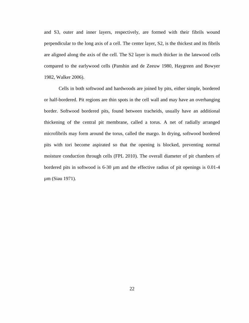
22

and S3, outer and inner layers, respectively, are formed with their fibrils wound

perpendicular to the long axis of a cell. The center layer, S2, is the thickest and its fibrils

are aligned along the axis of the cell. The S2 layer is much thicker in the latewood cells

compared to the earlywood cells (Panshin and de Zeeuw 1980, Haygreen and Bowyer

1982, Walker 2006).

Cells in both softwood and hardwoods are joined by pits, either simple, bordered

or half-bordered. Pit regions are thin spots in the cell wall and may have an overhanging

border. Softwood bordered pits, found between tracheids, usually have an additional

thickening of the central pit membrane, called a torus. A net of radially arranged

microfibrils may form around the torus, called the margo. In drying, softwood bordered

pits with tori become aspirated so that the opening is blocked, preventing normal

moisture conduction through cells (FPL 2010). The overall diameter of pit chambers of

bordered pits in softwood is 6-30 µm and the effective radius of pit openings is 0.01-4

µm (Siau 1971).

23

Figure 2-4: Cut-away drawing of a cluster of cells, including structural details of a

bordered pit. In the middle cell, the various layers of the cell wall are detailed at the

top of the drawing, beginning with the middle lamella (ML). The next layer is the

primary wall (P), and on the surface of this layer the random orientation of the

cellulose microfibrils is detailed. Interior to the primary wall is the secondary wall

in its three layers: S1, S2, and S3. The mirofibril angle of each layer is illustrated, as

well as the relative thickness of the layers. The lower portion of the illustration

shows bordered pits in both sectional and face view. (FPL 2010)

24

2.3 Water in wood

Water in wood has significant effects on all wood properties including physical

and mechanical properties. Therefore, interactions between wood and water influence all

steps of the production chain and the final product quality. For example, MC variations in

wood cause unequal shrinkage. Excessive moisture increases the cost of transportation

and decreases the amount of available thermal energy by hindering combustion (FPL

2010).

Once a tree is harvested, wood MC decreases due to drying. During the drying

process, regardless of the species, the water moves from a high concentration zone to a

lower concentration by capillary forces and diffusion. Such diffusion produces an

increase in the MC variation in the sample. Impermeable regions also generate MC

variations. For most species, the sapwood is permeable, so its drying rate is higher than

impermeable regions such as heartwood. Also, some species, such as fir, contain wet

pockets. These impermeable zones decrease the drying rate and require careful attention

during the drying process (Kroll et al. 1992; Cai 2006; Bowyer et al. 2007; Watanabe et

al. 2012b).

In green wood, water in the cell walls, is typically 25 to 35% of the mass of the

solid wood. It is well known (Siau 1971) that as wood dries, lumen water is removed first

followed by the cell wall water. Typically, the wood shrinks by about 7 to 17% in volume

as cell wall water is removed by diffusion. Capillary forces determine the movement of

lumen water. As wood dries, evaporation of water from the surface sets up capillary

forces that exert a pull on the lumen water in zones beneath the surface (Panshin and de

25

Zeeuw 1980, Spolek and Plumb 1981, Skaar 1988). When there is no lumen water in the

wood, capillary forces are no longer of importance. The fiber saturation point (FSP) is the

condition wherein the cell wall is assumed to be saturated with water but there is no

lumen water. More practically, the FSP is defined as the MC where abrupt changes in the

physical properties of wood occur (Stamm 1964).

A number of physical and mechanical properties of wood are independent of MC

at higher MCs above FSP, but these properties are found to change at lower MCs below

FSP as the cell wall water is removed (Siau 1971, Nelson 1986, FPL 2010). For example:

(i) The heat required to evaporate a unit weight of lumen water from wood is the heat of

vaporization of lumen water while there is an extra amount of heat, the heat of wetting,

that is needed to remove all the cell wall water (Stamm 1964, Bodig and Jayne 1982, Siau

1984), (ii) The mechanical strength of wood increases as the cell wall water is removed,

but is not affected by the amount of lumen water, (iii) The thermal and electrical

conductivities of wood are also altered by the removal of cell wall water but they are

independent of the amount of lumen water. Engelund et al. (2013) presented a

comprehensive review of the physics of wood-water interactions.

Cell wall water is closely associated with the cell-wall constituents through

hydrogen bonding. The most important element of cell wall water adsorption in wood

involves replacing solid-solid interfaces by solid-liquid-solid interfaces, and as a result

adsorption of water swells wood by forming a solid solution. In the hygroscopic range

(between 0% and FSP), the relationship between equilibrium MC of wood and relative

humidity at a given temperature is called the sorption isotherm.

26

It has been shown that the sorption isotherm of wood is of a sigmoidal shape and

has been classified as a type II isotherm (Stamm 1964, Siau 1984, Skaar 1988). The cell

wall water is generally considered to consist of two components, one strongly attracted,

the other weakly attracted by the sorption sites (Stamm 1964, Simpson 1973, Skaar

1988). When the sorption process is considered to be a surface phenomenon, the strongly

bound water is called monomolecular water whereas the weakly bound water is called

polymolecular water. When the sorption process is considered a solution phenomenon,

they are called water of hydration and water of solution, respectively.

In MR, the monomolecular water and polymolecular water would be considered

bound and free water, respectively. In both cell wall water and lumen water there will be

a surface monomolecular water layer and bulk like polymolecular water layers. The

surface monomolecular water and the bulk like polymolecular water will have different

MR relaxation lifetimes because of different water mobilities.

The wood science nomenclature for water in wood states that water can exist as

either free water in the cell lumens and intercellular spaces or as bound water within the

cell walls. But this nomenclature is contradictory and inappropriate to describe MR

experiments in wood materials. The cell wall water will have two components,

monomolecular and polymolecular water, not one. The monomolecular water and

polymolecular water in the cell wall are considered bound and free, respectively, in the

MR description. Exactly the same description applies to lumen water where water can

also exist as surface and bulk water. The surface water in this case is considered bound

water and the bulk water is free water in the MR description. The rapid exchange of

water between surface and bulk is discussed further in Section 2.5 of this Chapter. The

27

different ratios of bound and free water (MR description) in the cell wall versus cell

lumen result in different MR lifetimes in the cell wall and cell lumen. Similarly the

different ratio of bound and free water in cell cavities of different physical sizes results in

different MR lifetimes.

The cell wall water, both the monomolecular and the polymolecular water,

behaves differently and has different thermodynamic properties compared to bulk or

lumen water (Berthold et al. 1996; Olsson and Salmen 2004). These authors reported that

freezing cell wall water did not form normal ice structures because of the influence of the

polar groups of the cell wall materials. Sparks et al. (2000) employed time-domain

reflectometry to measure the water content of frozen plant materials. They found that

more than 25% of the water in wood was not frozen even at temperatures of -15°C. They

attributed this to water in the cell wall.

Nakamura et al. (1981) introduced a nomenclature for water held by cellulosic

materials such as wood according to which water may be found in three different states:

lumen water, freezing cell wall water and non-freezing cell wall water. The concept was

further investigated and developed by Berthold et al. (1994, 1996, 1998). The division of

cell wall water into freezing and non-freezing components has been quantified using

Differential Scanning Calorimetry (DSC). The freezing cell wall water has been assumed

to be less confined by, and more loosely bound to, the cell wall than non-freezing cell

wall water, for example, as water clusters in line with theoretical considerations of

Hartley et al. (1992) and Hartley and Avramidis (1993). However, MR relaxometry

performed on wood did not reveal any bound water freezing down to -20°C in Norway

spruce sapwood for MCs close to FSP (Thygesen at al. 2010). But most importantly,

28

Zelinka et al. (2012) presented results indicating that the DSC peak interpreted as

freezing bound water in cellulosic materials is consistent with homogeneous nucleation

of free water. Further, they showed that this DSC peak only occurred for isolated ball-

milled cellulose, not for solid wood or milled wood.

2.4 Conventional MC measurement techniques

The most common MC measurement methods employed by foresters, wood

scientist and forest industry practitioners are discussed below. The most generally

acceptable method is the gravimetric method, but it is destructive and time consuming.

Distillation is employed in MC measurements for species with large amounts of volatile

materials and for treated wood products. Electrical sensors and microwave moisture

sensors are also common in the industry.

2.4.1. Gravimetric (oven-dry basis)

In the wood products industry, the amount of water is expressed as the percentage

of the oven-dry weight by:

𝑀𝐶 (%) = 𝑀𝑔− 𝑀𝑜𝑑

𝑀𝑜𝑑 × 100 (Equation 2.1)

where Mg (kg) is the mass of the moist (green) wood sample and Mod (kg) is the

mass of the oven-dry wood. It should be noted that the MC is expressed as a percentage

of the oven-dry weight rather than as a percentage of the original weight. There are two

reasons for adopting this definition: (i) The industry is concerned primarily with the

amount of wood in a log. The moisture within the log is of no value, and (ii) The oven-

29

dry weight provides a stable reference point. This calculation of MC may result in a MC

value greater than 100%. The widely accepted method to measure MC is to weigh the wet

sample and then dry it in an oven for 24 hours at 103 ± 2°C to remove all water. The

oven-dried sample is then re-weighed. More information about this process can be found

in method A of ASTM-D4442-07 (2007).

The gravimetric measurement is destructive, it involves a measurement time on

the order of a day, and there is a practical limit to the size and number of pieces that can

be measured. Volatile constituents are removed during the drying process, which causes

small errors in MC calculations. Gravimetric methods of this type are commonly

employed in the industry and are considered the gold standard.

2.4.2. Gravimetric (green basis)

In some applications, the wood MC is defined based on the percentage of total

weight, which is the weight of green or wet wood (Equation 2.2). This calculation is

suitable for the fuel and the pulp and paper industries (Bowyer et al. 2007).

𝑀𝐶𝑤 (%) = 𝑀𝑔−𝑀𝑜𝑑

𝑀𝑔 × 100 (Equation 2.2)

There are many factors contributing to MC variations. In a living tree, the water

weight can be equal to or greater than the dry wood substance weight. Moreover, the

water distribution is not homogeneous in tree trunks. In green softwoods, the MC of

sapwood is usually greater than that of heartwood. In green hardwoods, the difference in

MC between heartwood and sapwood depends on the species (FPL 2010).

30

2.4.3. Distillation method

If wood has been treated or impregnated with chemicals, oven drying moisture

measurements may be inaccurate. An impregnant that is volatile at oven temperatures

will evaporate during oven drying, and the resulting weight loss can be misinterpreted as

due to evaporated water. An impregnant that is nonvolatile will remain in the wood and

so increase the apparent oven dry weight of the wood. For treated wood, the distillation

method may be more accurate than oven drying for measuring MC. In this method, water

is removed from the wood specimen in a closed system, in which the water is collected

and measured directly. The distillation method is more accurate than the oven dry method

for species that naturally contain large amounts of volatile materials other than water

(ASTM D4442-07).

As with gravimetric methods, distillation is a time consuming and destructive

measurement. In addition it requires considerable experimental skill. These problems

reinforce the need for alternate methods to measure MC.

2.4.4. Electrical moisture meters

Electrical moisture meters provide a quick and reasonably accurate measurement

of MC. There are three types of electric moisture meters, each based on the fundamental

relationship between MC and a different electric property: (i) The conductance-type

(resistance-type), uses the relationship between MC and direct current conductance; (ii)

The power-loss type, uses the relationship between MC and the dielectric loss factor of

the wood; and (iii) The capacitance type, which uses the relationship between MC and

the dielectric constant of the wood. The latter two types of meters are classed as dielectric

31

types (James 1988). The simplicity of electrical measurements of MC means that these

meters are commonly employed in the industry.

Direct current resistance moisture meters are more common. In these meters pair

of needles (electrodes), a fixed distance apart, is driven into the wood across or along the

grain and the electrical resistance measured. The measured MC is valid in close

proximity to the needles and cannot be generalized to the whole sample. The local

measurement is reasonably accurate between the FSP and approximately 6% MC.

Electric moisture meters provide a quick estimation of MC, but their accuracy is low for

samples with MC above 25%. Resistance meters are calibrated for a particular species

and manufacturers advise correction factors to apply for other species (James 1988; Skaar

1988). With electrodes driven into the wood, this method is considered destructive for

some wood applications (such as veneers and furniture).

Power-loss type meters use the relation between MC and loss factor. The wood

specimen is penetrated by the electric field radiating from an electrode that is coupled to

a low-power oscillator in the meter. Power absorbed by the specimen loads the oscillator

and reduces its amplitude of oscillation, which is in turn indicated by the meter dial.

Since the loss factor depends on MC, the meter reading can be related to percent MC

(James 1988). Calibration of these meters is species dependent.

The capacitance-type moisture meters use the relationship between MC and

dielectric constant. The wood specimen is penetrated by the electric field associated with

capacitance of the frequency–determining circuit of an oscillator when the electrode of

the meter contacts the wood. Good contact between the electrode and wood is important

for MC measurement. The frequency of the oscillator is changed according to the

32

dielectric constant of the wood specimen. A frequency discriminator generates a signal,

read on a meter, proportional to the change in frequency. Using the relation between

dielectric constant and moisture, the meter can be calibrated to read MC. The calibration

of these meters is species dependent.

2.4.5. Microwave moisture meters

Absorption of microwave radiation is employed in the wood industry to measure

MC. As the dielectric constant of water is higher than other materials, the signal

attenuation is dominated by water. This attenuated signal is measured by a detector and is

converted, at the correct microwave frequency, into a MC reading. Improvements in

microwave technology have prompted additional wood property measurement

opportunities (Tiuri at al. 1980, King et al. 1985, Martin et al. 1987, Leicester and Seath

1996). When a microwave beam propagates through wood, it is depolarized, attenuated

and undergoes a phase shift. These three changes, all of them directly measurable, depend

on the wood grain direction, MC, and dry density, respectively (Torgovnikov 1993). The

three microwave measurements can be undertaken simultaneously (King et al. 1985).

However, the spatial resolution in microwave systems is in the order of several

centimeters which precludes a thorough examination of drying mechanisms in wood.

Also, there is significant attenuation of the microwave signal at high frequency. The

attenuation is significant that it is no longer useful for MC measurements in green wood.

The power needed to overcome the attenuation is so high that it would heat or even burn

the wood.

33

2.5 Magnetic resonance

MR is a physical phenomenon in which magnetic nuclei are excited by radio

frequency (RF) magnetic fields and then detected by induction. The MR phenomenon

occurs at a specific frequency, the resonance frequency, which depends on the strength of

the magnetic field and on the magnetic properties of the isotope in question. According to

the Larmor equation, the resonance frequency is linearly dependent on both the strength

of the magnetic field and a nuclear property known as the gyromagnetic ratio (Liang and

Lauterbur 2000).

𝜔 = γB0 (Equation 2.3)

where 𝜔 is the resonance frequency also known as the Larmor frequency (MHz),

γ is the gyromagnetic ratio (42.58 MHz/Tesla in the case of 1H), and B0 is the static

magnetic field strength (Tesla).

The net magnetization, M0, measured with a magnetic resonance experiment, has

a magnitude of:

𝑀0 = 𝑁 𝐼(𝐼+1)𝛾2ħ2

3𝑘𝐵𝑇 𝐵0 (Equation 2.4)

where N is the total number of nuclei in the sample. The net magnetization

increases with an increase in external magnetic field strength or a decrease in temperature

(T). I is the spin quantum number which is equal 1/2 in the case of hydrogen. ħ = h/2π

where h is the Planck’s constant and kB is Boltzmann’s constant. The MR signal therefore

is proportional to the amount of H nuclei in the case of water, which will be MC when

normalized by total mass.

34

In MR, the term relaxation describes specific processes by which nuclear

magnetization in a non-equilibrium state returns to equilibrium. Two different time

constants characterize the longitudinal (spin-lattice) and transverse (spin-spin)

relaxations. The spin-lattice relaxation time T1 is a measure of the time required for a spin

system to return to thermal equilibrium with its surroundings (lattice). T1 governs the

recovery of the longitudinal magnetization. T2 (spin-spin relaxation time) is a measure of

the decay time of a transverse magnetization due to spin-spin interactions. T2∗ accounts

for the effect of both T2 decay and magnetic field inhomogeneities (Liang and Lauterbur

2000). The MR signal typically decays exponentially with T2 and T2∗ lifetimes which are

related to the type of water in wood. Imaging is spatial resolution of M0 with potential

image contrast related to T1, T2 or T2∗.

2.5.1. Free induction decay measurement

A free induction decay (FID) is the signal measured after an RF pulse as the

transverse magnetization decays. The effective T2 time constant, measured with a FID, is

T2∗.

1

𝑇2∗ =

1

𝑇2+ 𝛾Δ𝐵0 (Equation 2.5)

T2∗ relaxation depends on T2, the transverse relaxation time, and Δ𝐵0, which describes the

inhomogeneity of the static magnetic field.

2.5.2. Carr-Purcell-Meiboom-Gill measurement

The Carr-Purcell (Carr and Purcell 1954) measurement begins with a 90° pulse

followed by a series of 180° pulses. The initial 90° pulse rotates the magnetization into

35

the transverse plane. The first 180° pulse is applied after a time τ and inverts the phase of

the magnetization as it loses coherence. After a time 2τ the phase will achieve coherence,

resulting in signal called a spin echo (Hahn 1950). The transverse magnetization will lose

phase coherence once more, but can be regained with another 180° pulse. Therefore, a

train of 180° pulse creates a train of spin echoes that form midway between the 180°

pulses. The magnitude of the spin echoes decays with relaxation time T2, so T2 can be

determined through:

𝑀𝑥𝑦 = 𝑀0𝑒−𝑛𝑇𝐸/𝑇2 (Equation 2.6)

where TE = 2τ, the time between two successive 180° pulses and n is the echo

number. In practice, the 180° pulses are phase shifted to minimize artifacts caused by

successive imperfect 180° pulses. This modification was proposed by Meiboom and Gill

(1958) and is therefore known as the Carr-Purcell-Meiboom-Gill (CPMG) measurement.

Again, M0 is the net magnetization and it is proportional to the amount of H nuclei in the

case of water.

2.5.3 Surface and bulk water exchange

For porous media such as wood, where water is present in lumen, void spaces, or

trapped in micro pores, the spin-spin relaxation rate (1

𝑇2) is expressed as the weighted sum

of the surface relaxation rate and the bulk water relaxation rate (Wong 1999). In the case

of rapid exchange of water between the two environments, the mean relaxation rate is:

1

𝑇2=

𝑛

𝑇2 𝑆+

𝑚

𝑇2 B , 𝑛 + 𝑚 = 1 (Equation 2.7)

36

where 1

𝑇2 𝑆 is the surface relaxation rate, and the

1

𝑇2 𝐵 is the bulk water relaxation

rate, n and m are the relative quantities of surface and bulk water. Rapid exchange is

usually assumed for pore scale behavior as is the case for water in wood materials.

The observed relaxation rate from water in the lumen is the weighted average rate

of both the surface and bulk water, as given in Equation 2.5 (Wong 1999). Typically,

there is more bulk water than surface water when the wood is green, but the surface

relaxation rate is much greater than the bulk relaxation rate. This phenomenon is also true

for cell wall water wherein the monomolecular and polymolecular water can exchange

rapidly in a MR experiment. Changes in the ratio of the two populations will result in an

altered T2. Thus we anticipate a T2 for cell wall water that is different from the T2 of

lumen water with the lumen water T2 much longer. We may also then anticipate different

lumen T2 values for lumen cavities of different sizes, for example earlywood and

latewood.

2.6 Review of MR studies of water in wood

The wide-line 1H NMR absorption spectrum (Nanassy 1974) of wood exhibits a

narrow water line superimposed on a broad line from hydrogens of solid wood fiber. The

narrow line amplitude scaled with the amount of water, but was broader than that of pure

water, implying that water in wood was less mobile than bulk water.

It was demonstrated that the solid wood and water 1H NMR FID signal are

separable (Sharp et al. 1978, Riggin et al. 1979, Menon et al. 1987). The solid component

can be fitted to a second moment expansion to give an absolute MC measurement by 1H

NMR (Menon et al. 1987). Furthermore, the water signal could be separated on the basis

37

of T2 into cell wall water and lumen water (His et al. 1977, Riggin et al. 1979, Menon et

al. 1987). Further investigation of western red cedar (Flibotte et al. 1990) showed that the

solid wood signal has a second moment of about 5 x 109 s

-2 which increased by about

20% at low moisture contents below the FSP. Hartley et al. (1994) demonstrated the

effectiveness of the pulsed NMR in determining the absolute MC of aspen below FSP.

Heartwood and juvenile wood were found to have substantially less water and shorter cell

wall water T2 relaxation times than the sapwood, which enabled the sapwood-heartwood

boundary to be distinguished in a cross sectional MRI image of a cedar log, but the

heartwood-juvenile wood boundary was more difficult to discern. Decayed wood was

found to have high MC and so was easily identifiable, especially if in heartwood or

juvenile wood.

Pulsed field gradient diffusion measurements of water in wood (MacGregor et

al.1983, Peemoeller et al. 1985) showed that water in wood lumens undergoes restricted

diffusion in all directions, even in the long direction along the cell lumens. Water

squeezed from the wood was measured to have the same self-diffusion coefficient as free

water (MacGregor et al. 1983).

Water environments have been selectively imaged on the basis of T2 to produce

one-dimensional images of cell wall and lumen water separately. One-dimensional

images of earlywood, latewood and ray, and cell wall water for western red cedar were

acquired (Menon et al. 1989).

One-dimensional radial moisture profiles of western red cedar sapwood (Quick et

al. 1990), as a function of time during controlled air flow rate and temperature, showed

38

clearly that water removal as a function of time differs in the earlywood and latewood

regions. Three-dimensional imaging in whole body MRI scanners (Hall and

Rajanayagam 1986, Flibotte et al. 1990) was used to investigate water signal distribution

in wood. The echo time in conventional MRI is limited to about 20 ms, therefore only a

fraction of the water was imaged. Most MRI studies consider relatively wet wood

because conventional MRI techniques are not quantitative at low moisture contents.

However, MacMillan et al. (2002) demonstrated the use of Single Point Ramped Imaging

with T1 Enhancement MRI to image low MC wood samples.

Prior to this thesis work, there were no published MRI studies of freeze/thaw

behavior in solid wood. Several studies have been published employing bulk MR

measurements to examine freezing behaviors in wood (Gazdzizski et al. 2000, Thygesen

et al. 2010).

39

2.7 References



10.1520/D4442-07.

Berthier S, Kokutse AD, Stokes A, and Fourcaud T (2001) Irregular heartwood formation

in Maritime pine (Pinus pinaster Ait.): consequences for biomechanical and

hydraulic tree functioning. Ann Bot 87:19-25.

Berthold J, Desbrières J, Rinaudo M, and Salmén L (1994) Types of adsorbed water in

relation to the ionic groups and their counterions for some cellulose derivatives.

Polymer 35:5729-5736.

Berthold J, Rinaudo M, and Salmén L (1996) Association of water to polar groups;

estimations by an adsorption model for lingo-cellulosic materials. Colloid Surf A

112:117-129.

Berthold J, Olsson RJO, and Salmén L (1998) Water sorption to hydroxyl and carboxylic

acid groups in carboxymethylcellulose (CMC) studied with NIR-spectroscopy.

Cellulose 5:281-298.

Bodig J, and Jayne BA (1982). Mechanics of Wood and Wood Composites. Van

Nostrand and Reinhold, New York.

Bowyer JL, Shmulsky R, and Haygreen JG (2007) Forest products and wood science: An

Introduction. Oxford, UK: John Wiley & Sons. 496 pp.

Cai LP (2006) Using steam explosion to improve the dryability of wet pocket wood.

Forest Products Journal 56(7-8):75-78.

Carr HY, and Purcell EM (1954) Effects of diffusion on free precession in nuclear

magnetic resonance experiments. Phys Rev 94:630-638.

Engelund ET, Thygesen LG, Svensson S, and Hill CAS (2013). A critical discussion of

the physics of wood-water interactions. Wood Sci Technol 47:141-161.

Filbotte S, Menon RS, MacKay AL, and Hailey JRT (1990) Proton magnetic resonance

of western red cedar. Wood Fiber Sci 22(4):362-376.

Forest Products Laboratory (2010) Wood handbook - Wood as an engineering material.

Gen Tech Rep FPL-GTR-190. USDA Forest Services, Forest Products

Laboratory, Madison, WI. 509 pp.

40

Gartner BL, ed. (1995) Plant stems: Physiology and functional morphology, Academic

Press, Inc. San Diego, CA. 440 pp.

Gazdzizski S, Hartley ID, and Peemoeller H (2000) Freezing in trembling aspen (Populus

Tremuloides Michx.) by 1H NMR relaxometry. Molecular Physics Reports

29:144-146.

Hahn EL (1950) Spin Echoes. Phys Rev 80:580-584.

Hall LD, Rajanayagam V, Stewart WA, and Steiner PR (1986). Magnetic resonance

imaging of wood. Can J Forest Res 16(2):423-426.

Hartley ID, and Avramidis S (1993) Analysis of the wood sorption isotherm using

clustering theory. Holzforschung 47:163-167.

Hartley ID, Kamke FA, and Peemoeller H (1992) Cluster theory for water sorption in

wood. Wood Sci Technol 26:83-99.

Hartley ID, Kamke FA, and Peemoeller H (1994) Absolute moisture content

determination of aspen wood below the fiber saturation point using pulsed NMR.

Holzforschung 48(6):474-479.

Haygreen JG, and Bowyer JL (1982) Forest Products and Wood Science: An

Introduction, The Iowa State University Press, Ames, Iowa.

Hsi E, Hossfeld R, and Bryant RG (1977) Nuclear magnetic resonance relaxation study

of water absorbed on mill northern white-cedar. J Colloid Interface Sci 62:389-

395.

IAWA (1964) Multilingual glossary of terms used in wood anatomy. International

Association of Wood Anatomists, Committee on Nomenclature. Verlagsanstalt

Buchdruckerei Konkordia Winterthur, Switzerland. 186 pp.

James WL (1988) Electrical moisture meters for wood. USDA, Forest Service, Forest

Products Laboratory, General Technical Report FPL GTR-6.

King RJ, James WL, and Yen YY (1985) A microwave method for measuring moisture

content, density, and grain angle of wood. In: Proc 1st Intl Conference on

Scanning Technology in Sawmilling. Miller Freeman Publications, San Francisco,

CA.

Kroll RE, Ritter DC, Gertjejansen RO, and Au KC (1992) Anatomical and physical

properties of balsam poplar (Populus balsamifera) in Minnesota. Wood and Fiber

Science 24(1):13-24.

41

Leicester RH, and Seath CA (1996) Application of microwave scanners for stress

grading. In: 4th

Intl Wood Engineering Conference, New Orleans, 2:435-440.

Liang Z-P, and Lauterbur PC (2000) Principle of Magnetic Resonance Imaging – A

signal processing perspective. The Institute of Electrical and Electronics

Engineers, Inc., New York. pp. 57-76.

MacGregor RP, Peemoeller H, Schneider MH, and Sharp AR (1983) Anisotropic

diffusion of water in wood. J. Appl. Polym Sci 37:901-909.

MacMillan B, Schneider MH, Sharp AR, and Balcom BJ (2002) Magnetic resonance

imaging of water concentration in low moisture content wood. Wood Fiber

Science 2: 276-286.

Martin P, Collet R, Barthelemy P, and Roussy G (1987) Evaluation of wood

characteristics: internal scanning of the material by microwaves. Wood Sci

Technol 21(4):361-371.

Meiboom S, and Gill D (1958) Modified spin-echo method for measuring nuclear

relaxation times. Rev Sci Instr 29:688-691.

Menon RS, MacKay AL, Hailey JRT, Bloom M, Burgess AE, and Swanson JS (1987) An

NMR determination of the physiological water distribution in wood during

drying. J Appl Polym Sci 33:1141-1155.

Menon RS, MacKay AL, Flibotte S, and Hailey JRT (1989) Quantitative separation of

NMR images of water in wood on the basis of T2. J. Magn. Reson 82:205-210.

Nakamura K, Hatakeyama T, and Hatakeyama H (1981) Studies on bound water of

cellulose by differential scanning calorimetry. Text Res J 51:607-613.

Nanassy AJ (1974) Water sorption in green and remoistened wood studied by the broad-

line component of the wide-line NMR spectra. Wood Science 7(1):61-68.

Nelson RM Jr. (1986) Diffusion of bound water in wood. Wood Sci. Technol. 20:235-

251.

Olsson AM, and Salmén L (2004) The association of water to cellulose and hemicellulose

in paper examined by FTIR spectroscopy. Carbohydrate Research (339):813-818.

Panshin AJ, and de Zeeuw C (1980) Textbook of Wood Technology. 4th

Ed. McGraw-

Hill Publishing Company. pp. 722.

42

Quick JJ, Hailey JRT, and MacKay AL (1990) Radial moisture profiles of cedar sapwood

during drying: A proton magnetic resonance study. Wood Fiber Sci 22(4):404-

412.

Riggin MT, Sharp AR, Kaiser R, and Schneider MH (1979) Transverse NMR Relaxation

of water in wood. Journal of Applied Polymer Science 23:3147-3154.

Ryan MG (1989) Sapwood volume for three subalpine conifers: predictive equations and

ecological implications. Can. J. For. Res. 19:1397-1401.

Sharp AR, Riggin MT, Kaiser R, and Schneider MH (1978) Determination of moisture

content of wood by pulsed nuclear magnetic resonance. Wood Fiber Science

10:74-81.

Siau JF (1971) Flow in Wood. 1st Ed. Syracuse University Press, Syracuse, New York.

pp. 131.

Simpson WT (1973) Predicting equilibrium moisture content of wood by mathematical

models. Wood Fiber. 5:41-49.

Skaar C (1988) Wood-water relations. Springer-Verlag, New York. 283 pp.

Sparks JP, Campbell GS, and Black RA (2000) Liquid water content of wood tissue at

temperatures below 0oC. Can J Forest Res 30 (4):624-630.

Spolek GA, and Plumb OA (1981) Capillary pressure in softwoods. Wood Sci. Technol.

15:189-199.

Stamm AJ (1964) Wood and Cellulose Science. The Ronald Press Company, New York,

USA. 549 pp.

Thygesen LG, Engelund ET, and Hoffmeyer P (2010) Water sorption in wood and

modified wood at high values of relative humidity – Part 1: results for untreated,

acetylated, and furfurylated Norway spruce. Holzforschung 64:315-323.

Tiuri M, Jokela K, and Heikkila S (1980) Microwave instrument for accurate moisture

and density measurement of timber. J. Microwave Power 15:251-254.

Torgovnikov GI (1993) Dielectric properties of wood and wood-based materials,

Springer-Verlag, New York.

Walker JCF (2006) Primary Wood Processing: Principles and Practice. 2nd

Ed. Springer,

Dordrecht, Netherlands. 603 pp.

43

Watanabe K, Mansfield SD, and Avramidis S (2012b) Wet-pocket classification in Abies

lasiocarpa using spectroscopy in the visible and near infrared range. European

Journal of Wood and Wood Products 70:61-67.

Zelinka SL, Lambrecht MJ, Glass SV, Wiedenhoeft AC, and Yelle DJ (2012)

Examination of water phase transitions in Loblolly pine and cell wall components

by differential scanning calorimetry. Thermochim Acta 533:39-45.

Zobel BJ, and Sprague JR (1998) Juvenile Wood in Forest Trees. Springer Series in

Wood Science. Springer Berlin Heidelberg. 300 pp.

44

Chapter 3 – Examination of water phase transitions in black spruce by

magnetic resonance and magnetic resonance imaging

During the winter season when wood logs are exposed to freezing conditions, it is

vital to know whether MC measuring devices can estimate water content of frozen wood

samples. This chapter shows that frozen water cannot be measured with MR, however,

the UMR works well for measuring water in thawed wood. The goal was to observe and

understand the behaviour of water below 0°C in solid wood.

This chapter is largely based on the paper “Examination of water phase transitions

in black spruce by magnetic resonance and magnetic resonance imaging” published in the

Wood and Fiber Science Journal (Lamason et al. 2014). The format of references in this

chapter follows that of the original article. This paper was awarded second place in the

2015 George Marra award for excellence in writing and research competition, by the

Society of Wood Science and Technology, USA.

In this chapter, the author employed the conventional wood science nomenclature

for bound and free water. This chapter and publication were written in the early stages of

this project. For later chapters the author of this thesis employed an alternate description

of the water environment in wood materials that is more suitable for magnetic resonance

and is more precise. This alternate description was also employed in Chapter 2 of this

thesis, the theory and background chapter.

45

3.1 Introduction

Wood is a hygroscopic and anisotropic material whose properties are deeply

influenced by the presence of water. Measurements of moisture content (MC) of wood

are therefore of considerable importance. Water in wood can exist as either absorbed

water (free water) in the cell lumens and intercellular spaces or as adsorbed water (bound

water) within the cell walls (Siau 1971, Panshin and de Zeeuw 1980, Walker 2006). The

fiber saturation point (FSP) is defined as the MC at which all the absorbed water has been

removed but the cell walls are still fully saturated. This occurs around 30% MC for most

species (Skaar 1988, Walker 2006). The FSP is a critical parameter since most properties

of wood are altered by changes in MC below the FSP. A number of physical and

mechanical properties of wood are independent of MC at higher MCs above FSP, but

these properties are found to change at lower MCs, below FSP, as the bound water is

removed (Siau 1971 and FPL 2010). For example, wood shrinks as bound water is

removed.

Numerous magnetic resonance (MR) and magnetic resonance imaging (MRI)

studies on wood have been reported in the literature. Conventional MR and MRI

techniques were employed to study wood anatomy and structure (Wang and Chang 1986,

Hall et al 1986, Filbotte et al. 1990), wood decay (Filbotte et al. 1990), and wood

preservation (Meder et al. 1999). With respect to MC estimation, MR/MRI techniques

have been employed to estimate MC in wood pellets (Nyström and Dahlquist 2004) and

in wood drying (Hall et al. 1986, Menon et al. 1989, Quick et al. 1990, Araujo et al. 1992,

Hartley et al. 1994, Hameury et al. 2006, Almeida et al. 2007, Stenstrom et al. 2009).

Most MRI studies consider relatively wet wood because conventional MRI techniques

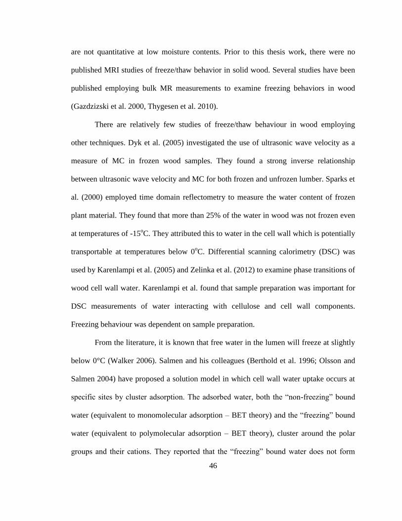
46

are not quantitative at low moisture contents. Prior to this thesis work, there were no

published MRI studies of freeze/thaw behavior in solid wood. Several studies have been

published employing bulk MR measurements to examine freezing behaviors in wood

(Gazdzizski et al. 2000, Thygesen et al. 2010).

There are relatively few studies of freeze/thaw behaviour in wood employing

other techniques. Dyk et al. (2005) investigated the use of ultrasonic wave velocity as a

measure of MC in frozen wood samples. They found a strong inverse relationship

between ultrasonic wave velocity and MC for both frozen and unfrozen lumber. Sparks et

al. (2000) employed time domain reflectometry to measure the water content of frozen

plant material. They found that more than 25% of the water in wood was not frozen even

at temperatures of -15oC. They attributed this to water in the cell wall which is potentially

transportable at temperatures below 0oC. Differential scanning calorimetry (DSC) was

used by Karenlampi et al. (2005) and Zelinka et al. (2012) to examine phase transitions of

wood cell wall water. Karenlampi et al. found that sample preparation was important for

DSC measurements of water interacting with cellulose and cell wall components.

Freezing behaviour was dependent on sample preparation.

From the literature, it is known that free water in the lumen will freeze at slightly

below 0°C (Walker 2006). Salmen and his colleagues (Berthold et al. 1996; Olsson and

Salmen 2004) have proposed a solution model in which cell wall water uptake occurs at

specific sites by cluster adsorption. The adsorbed water, both the “non-freezing” bound

water (equivalent to monomolecular adsorption – BET theory) and the “freezing” bound

water (equivalent to polymolecular adsorption – BET theory), cluster around the polar

groups and their cations. They reported that the “freezing” bound water does not form

47

normal ice structures due to the influence of the polar groups of the cell wall materials,

and this water has non bulk-water-like thermodynamic parameters

The purpose of the current study was to further investigate the behavior of water

in wood at low temperatures with magnetic resonance and magnetic resonance imaging.

In particular, we were interested in the phase transitions of water in black spruce (Picea

mariana Mill.). These were investigated with standard bulk MR, with MRI, and with

unilateral MR, a new instrumental approach with increased flexibility and portability. It is

our aim to demonstrate that MR and MRI are well suited to quantify water content of

frozen and thawed black spruce wood samples and thereby to observe phase changes in

temperature dependent measurements. In this work we assume that MR and MRI signal

intensities are not affected by any changes in FSP and other chemical effects on wood at

low temperatures. Likewise, changes in FSP at freezing conditions are assumed to be

very minimal. Similar studies have been undertaken in other porous materials, notably the

MRI study by Prado et al. (1998) on freeze/thaw behaviours of concrete.

3.2 MR and MRI background

MR is a physical phenomenon in which nuclei with a magnetic moment are

excited by radio frequency (RF) magnetic fields and then detected by induction in the RF

probe. The MR phenomenon occurs at a specific frequency, the resonance frequency,

which depends on the strength of the magnetic field and on the magnetic properties of the

nuclei under study. According to the Larmor equation, the resonance frequency is directly

48

dependent on both the strength of the magnetic field and the gyromagnetic ratio (Liang

and Lauterbur 2000).

𝜔 = γB0 (Equation 3.1)

where 𝜔 is the resonance frequency also known as the Larmor frequency (MHz).

The gyromagnetic ratio (γ) is a constant dependent on the nuclei under study, 42.58

MHz/Tesla for 1H. B0 is the static magnetic field strength (Tesla).

In MR, the term relaxation describes specific processes by which nuclear

magnetization in non-equilibrium states returns to equilibrium. Two different time

constants characterize the longitudinal (spin-lattice) and transverse (spin-spin)

relaxations. T1 (spin-lattice relaxation time) is a measure of the time required for a spin

system to return to thermal equilibrium with its surroundings (lattice). T1 governs the

recovery of the longitudinal magnetization. T2 (spin-spin relaxation time) governs the

decay of transverse magnetization due to spin-spin interactions. 𝑇2∗ accounts for the effect

of both T2 decay and magnetic field inhomogeneities (Liang and Lauterbur 2000). The

MR signal typically decays exponentially with T2 and 𝑇2∗ which are related to the type of

water (bound and free) in wood.

For porous media such as wood, where water is present in void spaces, or trapped

in micro pores, the spin-spin relaxation rate (1

𝑇2) is expressed as the weighted sum of the

surface relaxation rate and the bulk relaxation rate (Wong 1999). In the case of rapid

exchange of water between the two environments, one observes an average relaxation

rate.

1

𝑇2=

𝑛

𝑇2 𝑆+

𝑚

𝑇2 𝐵 , 𝑛 + 𝑚 = 1 (Equation 3.2)

49

where 1


1

𝑇2 𝐵 is the bulk relaxation rate.

The variables n and m are the relative quantities of water in the surface and bulk

environments.

In the case of water in wood, there are three different water environments. (1)

Water in the cell walls is motionally restricted and conventionally considered bound

water. Stamm (1964) employed the sigmoidal adsorption curve proposed by Brunauer,

Emmett and Teller (1938), the BET equation, to calculate the average number of

molecular layers of water at fiber saturation. Stamm reported 6.5 layers for sitka spruce

(Picea sitchensis) and 7.5 layers for sugar maple (Acer saccharum). The moisture needed

to form a monomolecular surface layer within the amorphous regions of cellulose

corresponds to a moisture content of about 5% (Stamm 1964, Walker 2006). The BET

theory considered the cell wall water as a surface phenomenon, with a strongly adsorbed

monolayer and less strongly bound polymolecular water.

There are two different types of lumen water. One is the bulk lumen water (2)

which is considerably more mobile, and the other is a small fraction which adheres to the

lumen walls (3). The observed relaxation rate from the water in the lumen

(conventionally called free water) is the weighted average rate of the surface water and

bulk water, as given in equation 3.2 (Wong 1999). Typically, there is more bulk water

than surface water when the wood is green, but the surface relaxation rate is much larger

than the bulk relaxation rate. The bulk and surface water in the lumen together are

considered free water.

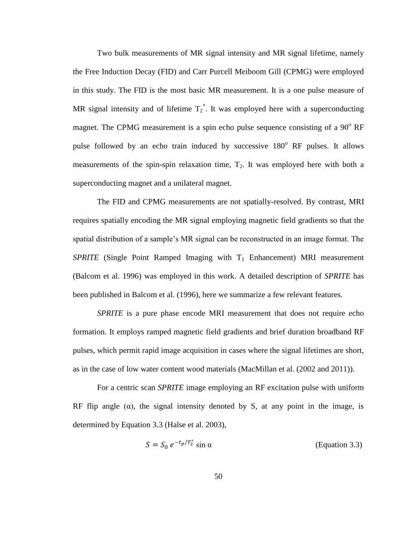
50

Two bulk measurements of MR signal intensity and MR signal lifetime, namely

the Free Induction Decay (FID) and Carr Purcell Meiboom Gill (CPMG) were employed

in this study. The FID is the most basic MR measurement. It is a one pulse measure of

MR signal intensity and of lifetime T2*. It was employed here with a superconducting

magnet. The CPMG measurement is a spin echo pulse sequence consisting of a 90o RF

pulse followed by an echo train induced by successive 180o RF pulses. It allows

measurements of the spin-spin relaxation time, T2. It was employed here with both a

superconducting magnet and a unilateral magnet.

The FID and CPMG measurements are not spatially-resolved. By contrast, MRI

requires spatially encoding the MR signal employing magnetic field gradients so that the

spatial distribution of a sample’s MR signal can be reconstructed in an image format. The

SPRITE (Single Point Ramped Imaging with T1 Enhancement) MRI measurement

(Balcom et al. 1996) was employed in this work. A detailed description of SPRITE has

been published in Balcom et al. (1996), here we summarize a few relevant features.

SPRITE is a pure phase encode MRI measurement that does not require echo

formation. It employs ramped magnetic field gradients and brief duration broadband RF

pulses, which permit rapid image acquisition in cases where the signal lifetimes are short,

as in the case of low water content wood materials (MacMillan et al. (2002 and 2011)).

For a centric scan SPRITE image employing an RF excitation pulse with uniform

RF flip angle (α), the signal intensity denoted by S, at any point in the image, is

determined by Equation 3.3 (Halse et al. 2003),

𝑆 = 𝑆0 𝑒−𝑡𝑝/𝑇2∗ sin α (Equation 3.3)

51

where S0, is the signal intensity at t = 0. S0 is proportional to the quantity of

observable water. tp is the phase encode time and 𝑇2∗ is the effective transverse signal

lifetime. 𝑇2∗ is a function of both the intrinsic transverse relaxation time, T2, and the local

magnetic field inhomogeneity ΔB0 as shown in Equation 3.4,

1

𝑇2∗ =

1

𝑇2+ 𝛾Δ𝐵0 (Equation 3.4)

where 𝛾 is the nuclear gyromagnetic ratio. Generally for water in wood, tp << 𝑇2∗

meaning that the SPRITE signal intensity does not suffer from 𝑇2∗ attenuation and the

signal intensity is directly proportional to liquid water content. It is important to point out

that 𝑇2∗ is long for liquids, but short for solids, so that when water freezes, the signal

intensity decreases dramatically (according to eq. 3), because tp >> 𝑇2∗. Frozen water, ice,

will not be visible in the image (Prado et al. 1998).

The SPRITE MRI measurement was employed with the superconducting magnet

instrument to resolve 3D space within the sample whereas the unilateral magnet

integrates signal from a finite volume within the sample. The superconducting magnet

instrument is a more mature technology than the unilateral magnet. SPRITE MRI

measurements were compared to the CPMG measurements employing the unilateral

magnet.

3.3 Materials and methods

Thawing and freezing measurements of MR signal were undertaken on black

spruce. Black spruce samples were collected from a small sawmill near the village of

Point Leamington in Newfoundland, Canada. For thawing studies, three black spruce

52

sapwood samples and one black spruce heartwood sample of approximately 2.5 cm x 7.5

cm x 7.5 cm were prepared from an initially frozen green wood disk. The top portion of

the sapwood sample contained the bark. The green wood disk was wrapped with

cellophane and kept in the freezer until the time of measurement to prevent moisture loss.

The sapwood samples had bark on the outer part of the sample. One of the sapwood

samples and the heartwood sample were used for imaging measurements, while the

remaining two sapwood samples were used for UMR measurements. The samples were

initially frozen at approximately -20°C, and then allowed to thaw, during the

measurements, at ambient temperature.

For thawing studies, bulk MR and MRI measurements were undertaken. The 3D

SPRITE MRI images were acquired employing a Nalorac 2.4 Tesla horizontal bore

superconducting magnet (Nalorac Cryogenics Inc., Martinez, CA) instrument. The

ambient temperature surrounding the sample was 12°C. SPRITE 3D imaging parameters

were: number of scans = 4, time between gradient steps = 2 ms, time between conical

gradient trajectories = 300 ms, encoding time = 112 µs, maximum gradient = 6 G/cm,

field of view (FOV) = 12 cm, RF pulse width = 10.0 µs, r.f. flip angle = 8°, total

acquisition time = 10 min.

The unilateral permanent magnet, designed and fabricated in the UNB MRI

Centre, is a lightweight 3 magnet array (Marble et. al. 2007) which offers open access

and portability. Figure 3-1 is a photograph of the unilateral magnet along with the RF

coil. Figure 3-2 is a plot of the magnetic field along the central vertical line above the

surface of the unilateral magnet employed in this study. The unilateral magnet has a

53

homogenous magnetic field of 1 cm3 volume located approximately 1.3 cm away from

the top of the magnet.

Figure 3-1: Photograph of the unilateral magnet device employed in this study. The

white circle on the face of the magnet array is the RF probe. The sensor is connected

to the Bruker Minispec console and the RF probe is placed adjacent to the wood

sample for moisture content measurements.

54

Figure 3-2: Magnetic field along the central vertical line of the magnet array. The

center of the homogeneous spot is 1.3 cm from the surface of the magnet. This

permits measurement of signal within a finite volume inside the sample and not just

on the surface. In the case of the black spruce sample tested, measurement of MR

signal in the sapwood was therefore possible without first removing the bark.

For the unilateral magnet measurements, the ambient temperature was 3°C. This

was achieved by placing the unilateral magnet and the sample inside an insulated and

actively cooled box in order to slow the thawing process. Measurements were taken

continuously until the sample thawed completely. Each sample was wrapped in

cellophane, and no significant mass loss was observed over the course of the

measurements. The CPMG measurement, undertaken on a 4.46 MHz resonance

55

frequency unilateral magnet instrument, was employed to measure the spin-spin

relaxation time (T2). CPMG measurement parameters were: 90° pulse length = 10µs,

scans = 512, number of echoes = 128 and acquisition time was about 5 min.

For freezing studies, we employed 2D Spiral SPRITE MRI measurements on a 0.3

cm x 2.5 cm x 2.5 cm sapwood sample with no visual defects. The sample was prepared

from the same ‘green’ wood disk as for the thawing study. The dimensions of the ‘small’

sapwood sample allowed it to fit a sample holder for temperature control. The ‘small’

sapwood sample permitted rapid and more uniform temperature changes as compared to

the original sample (2.5 cm x 7.5 cm x 7.5 cm) in the 3D SPRITE measurements. The

sample was wrapped in cellophane to prevent mass loss during the course of the

measurements. It was left at ambient temperature for approximately an hour before

commencement of the measurements. Sample mass was measured before and after

measurements and no significant mass loss was observed. For temperature control, the

sample was positioned in a heated/cooled air stream inside a glass transfer line specially

designed to fit the geometrical specifications of the imaging system. The air temperature

was controlled with an Omega (Omega Engineering, Stamford, CT) CN6072A-P2

temperature controller employing a platinum resistance temperature device (RTD) in

close proximity to the sample. The air temperature was stable to within ±0.3°C. MRI was

undertaken at temperatures which ranged from -1°C to -100°C.

2D Spiral SPRITE MRI (Szomolanyi et al. 2001) measurements were performed

during freezing. The SPRITE experimental parameters include: number of scans = 32,

time between gradient steps = 2 ms, time between spirals = 500 ms, encoding time = 72

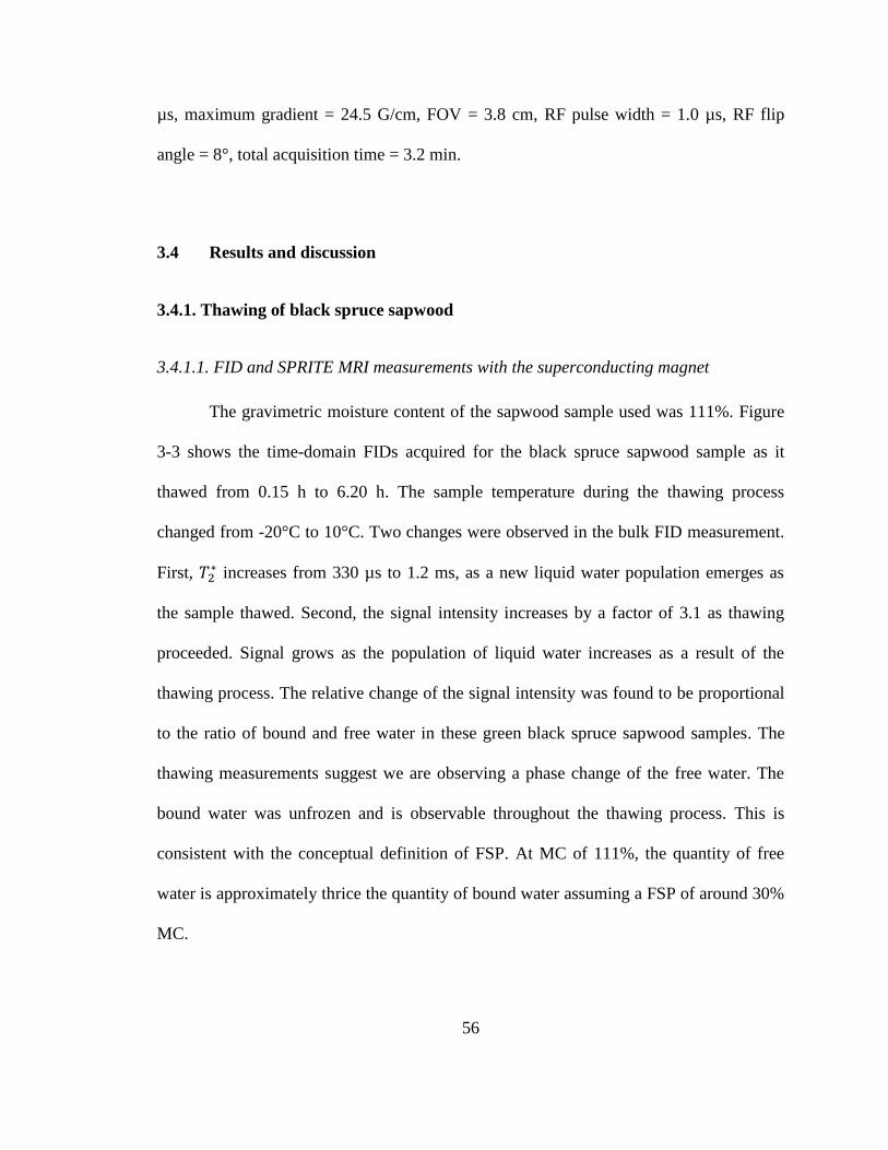
56

µs, maximum gradient = 24.5 G/cm, FOV = 3.8 cm, RF pulse width = 1.0 µs, RF flip

angle = 8°, total acquisition time = 3.2 min.

3.4 Results and discussion

3.4.1. Thawing of black spruce sapwood

3.4.1.1. FID and SPRITE MRI measurements with the superconducting magnet

The gravimetric moisture content of the sapwood sample used was 111%. Figure

3-3 shows the time-domain FIDs acquired for the black spruce sapwood sample as it

thawed from 0.15 h to 6.20 h. The sample temperature during the thawing process

changed from -20°C to 10°C. Two changes were observed in the bulk FID measurement.

First, 𝑇2∗ increases from 330 µs to 1.2 ms, as a new liquid water population emerges as

the sample thawed. Second, the signal intensity increases by a factor of 3.1 as thawing

proceeded. Signal grows as the population of liquid water increases as a result of the

thawing process. The relative change of the signal intensity was found to be proportional

to the ratio of bound and free water in these green black spruce sapwood samples. The

thawing measurements suggest we are observing a phase change of the free water. The

bound water was unfrozen and is observable throughout the thawing process. This is

consistent with the conceptual definition of FSP. At MC of 111%, the quantity of free

water is approximately thrice the quantity of bound water assuming a FSP of around 30%

MC.

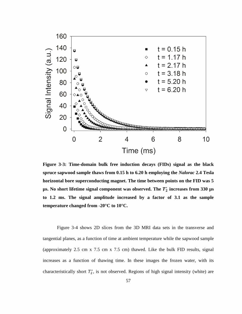
57

Figure 3-3: Time-domain bulk free induction decays (FIDs) signal as the black

spruce sapwood sample thaws from 0.15 h to 6.20 h employing the Nalorac 2.4 Tesla

horizontal bore superconducting magnet. The time between points on the FID was 5

µs. No short lifetime signal component was observed. The 𝑻𝟐∗ increases from 330 µs

to 1.2 ms. The signal amplitude increased by a factor of 3.1 as the sample

temperature changed from -20°C to 10°C.

Figure 3-4 shows 2D slices from the 3D MRI data sets in the transverse and

tangential planes, as a function of time at ambient temperature while the sapwood sample

(approximately 2.5 cm x 7.5 cm x 7.5 cm) thawed. Like the bulk FID results, signal

increases as a function of thawing time. In these images the frozen water, with its

characteristically short 𝑇2∗, is not observed. Regions of high signal intensity (white) are

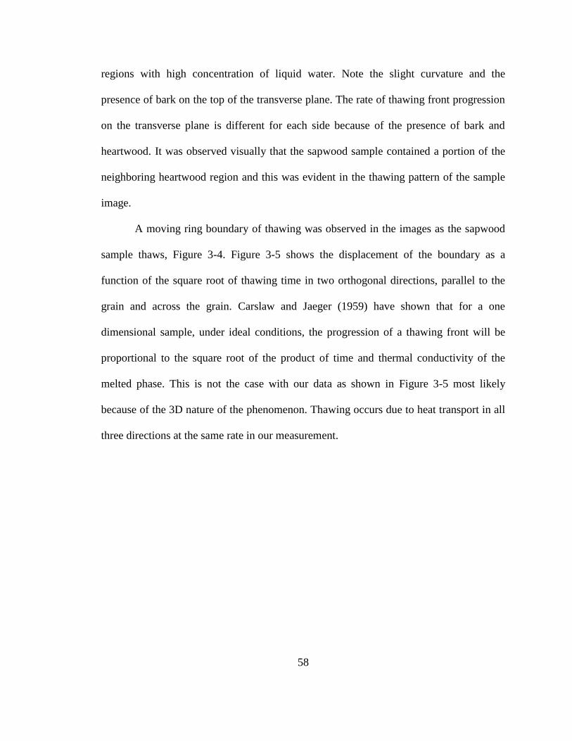
58

regions with high concentration of liquid water. Note the slight curvature and the

presence of bark on the top of the transverse plane. The rate of thawing front progression

on the transverse plane is different for each side because of the presence of bark and

heartwood. It was observed visually that the sapwood sample contained a portion of the

neighboring heartwood region and this was evident in the thawing pattern of the sample

image.

A moving ring boundary of thawing was observed in the images as the sapwood

sample thaws, Figure 3-4. Figure 3-5 shows the displacement of the boundary as a

function of the square root of thawing time in two orthogonal directions, parallel to the

grain and across the grain. Carslaw and Jaeger (1959) have shown that for a one

dimensional sample, under ideal conditions, the progression of a thawing front will be

proportional to the square root of the product of time and thermal conductivity of the

melted phase. This is not the case with our data as shown in Figure 3-5 most likely

because of the 3D nature of the phenomenon. Thawing occurs due to heat transport in all

three directions at the same rate in our measurement.

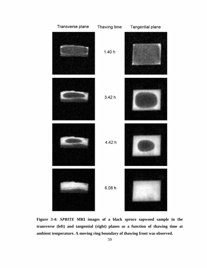
59

Figure 3-4: SPRITE MRI images of a black spruce sapwood sample in the

transverse (left) and tangential (right) planes as a function of thawing time at

ambient temperature. A moving ring boundary of thawing front was observed.

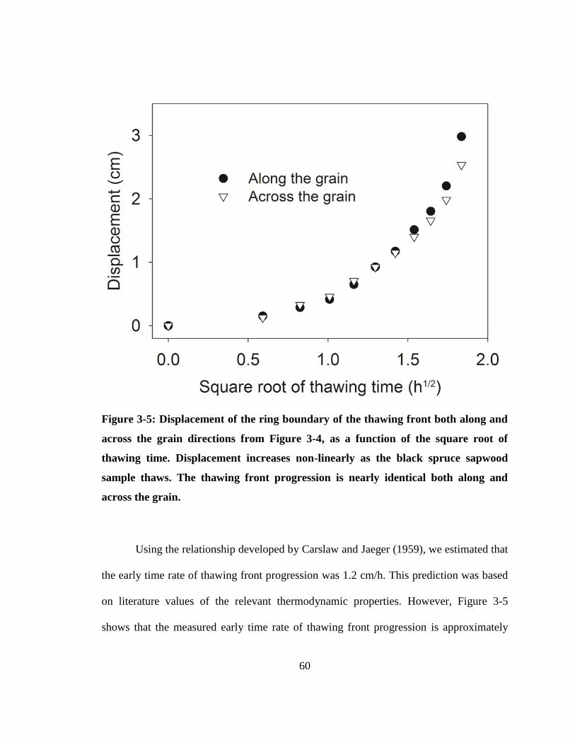
60

Figure 3-5: Displacement of the ring boundary of the thawing front both along and

across the grain directions from Figure 3-4, as a function of the square root of

thawing time. Displacement increases non-linearly as the black spruce sapwood

sample thaws. The thawing front progression is nearly identical both along and

across the grain.

Using the relationship developed by Carslaw and Jaeger (1959), we estimated that

the early time rate of thawing front progression was 1.2 cm/h. This prediction was based

on literature values of the relevant thermodynamic properties. However, Figure 3-5

shows that the measured early time rate of thawing front progression is approximately

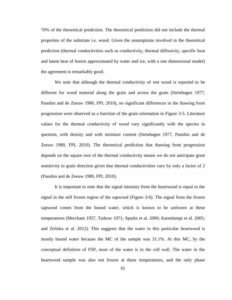
61

70% of the theoretical prediction. The theoretical prediction did not include the thermal

properties of the substrate i.e. wood. Given the assumptions involved in the theoretical

prediction (thermal conductivities such as conductivity, thermal diffusivity, specific heat

and latent heat of fusion approximated by water and ice, with a one dimensional model)

the agreement is remarkably good.

We note that although the thermal conductivity of wet wood is reported to be

different for wood material along the grain and across the grain (Steinhagen 1977,

Panshin and de Zeeuw 1980, FPL 2010), no significant differences in the thawing front

progression were observed as a function of the grain orientation in Figure 3-5. Literature

values for the thermal conductivity of wood vary significantly with the species in

question, with density and with moisture content (Steinhagen 1977, Panshin and de

Zeeuw 1980, FPL 2010). The theoretical prediction that thawing front progression

depends on the square root of the thermal conductivity means we do not anticipate great

sensitivity to grain direction given that thermal conductivities vary by only a factor of 2

(Panshin and de Zeeuw 1980, FPL 2010).

It is important to note that the signal intensity from the heartwood is equal to the

signal in the still frozen region of the sapwood (Figure 3-6). The signal from the frozen

sapwood comes from the bound water, which is known to be unfrozen at these

temperatures (Merchant 1957, Tarkow 1971; Sparks et al. 2000; Karenlampi et al. 2005;

and Zelinka et al. 2012). This suggests that the water in this particular heartwood is

mostly bound water because the MC of the sample was 31.1%. At this MC, by the

conceptual definition of FSP, most of the water is in the cell wall. The water in the

heartwood sample was also not frozen at these temperatures, and the only phase

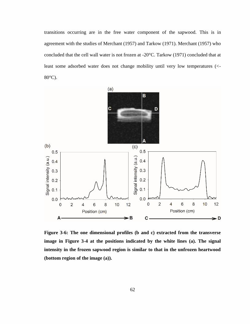
62

transitions occurring are in the free water component of the sapwood. This is in

agreement with the studies of Merchant (1957) and Tarkow (1971). Merchant (1957) who

concluded that the cell wall water is not frozen at -20°C. Tarkow (1971) concluded that at

least some adsorbed water does not change mobility until very low temperatures (<-

80°C).

Figure 3-6: The one dimensional profiles (b and c) extracted from the transverse

image in Figure 3-4 at the positions indicated by the white lines (a). The signal

intensity in the frozen sapwood region is similar to that in the unfrozen heartwood

(bottom region of the image (a)).

63

3.4.1.2. CPMG measurements employing unilateral magnet

The gravimetric moisture content of the sapwood sample employed for the

unilateral magnet measurements was 109%. A 2-component T2 fit was employed to

analyze the CPMG T2 decay data (Figure 3-7). The total signal increased as the sample

thawed. The liquid water population increased accordingly. Signal magnitude is

proportional to the amount of unfrozen water in the sample. The short and long lifetime

components correspond to the bound and free water, respectively. These results are in

agreement with Riggins et al. (1979) and Araujo et al. (1992), who reported relaxation

times of water in wood which corresponded to cell wall water and lumen water. The

moisture content is derived from the y-intercepts of Figure 3-7, with the help of a

calibration standard.

Figure 3-7 shows time-domain CPMG decay plots of signal intensity as sapwood

samples thawed to various extents. The time constant of the short lifetime component is

too short to measure accurately given the dead time of the RF probe (~ 120 µs)

employed. But based on the data points observed, the short T2 component is estimated to

be 0.5 – 0.9 ms. The long T2 components varied between 40.9 and 54.0 ms. Only the long

lifetime components were further analyzed.

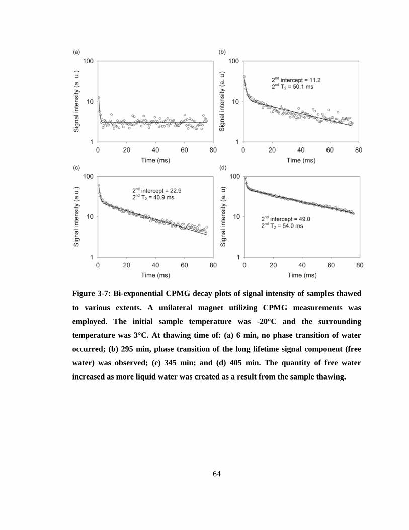
64

Figure 3-7: Bi-exponential CPMG decay plots of signal intensity of samples thawed

to various extents. A unilateral magnet utilizing CPMG measurements was

employed. The initial sample temperature was -20°C and the surrounding

temperature was 3°C. At thawing time of: (a) 6 min, no phase transition of water

occurred; (b) 295 min, phase transition of the long lifetime signal component (free

water) was observed; (c) 345 min; and (d) 405 min. The quantity of free water

increased as more liquid water was created as a result from the sample thawing.

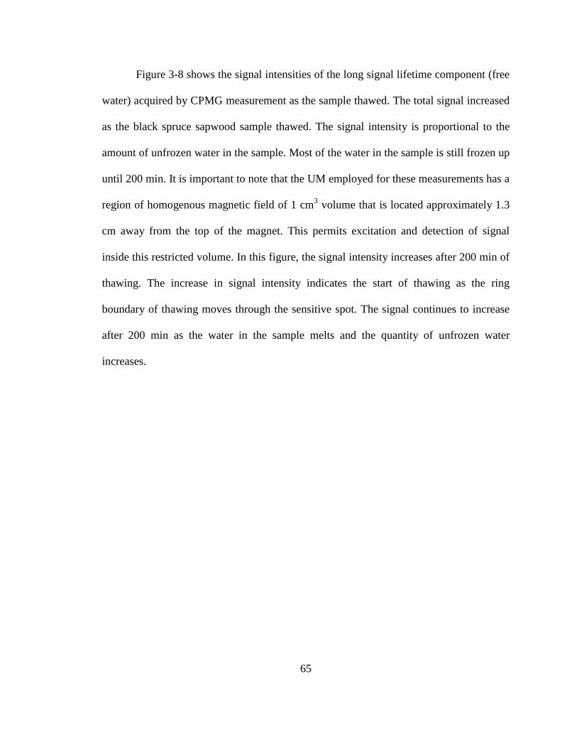
65

Figure 3-8 shows the signal intensities of the long signal lifetime component (free

water) acquired by CPMG measurement as the sample thawed. The total signal increased

as the black spruce sapwood sample thawed. The signal intensity is proportional to the

amount of unfrozen water in the sample. Most of the water in the sample is still frozen up

until 200 min. It is important to note that the UM employed for these measurements has a

region of homogenous magnetic field of 1 cm3 volume that is located approximately 1.3

cm away from the top of the magnet. This permits excitation and detection of signal

inside this restricted volume. In this figure, the signal intensity increases after 200 min of

thawing. The increase in signal intensity indicates the start of thawing as the ring

boundary of thawing moves through the sensitive spot. The signal continues to increase

after 200 min as the water in the sample melts and the quantity of unfrozen water

increases.

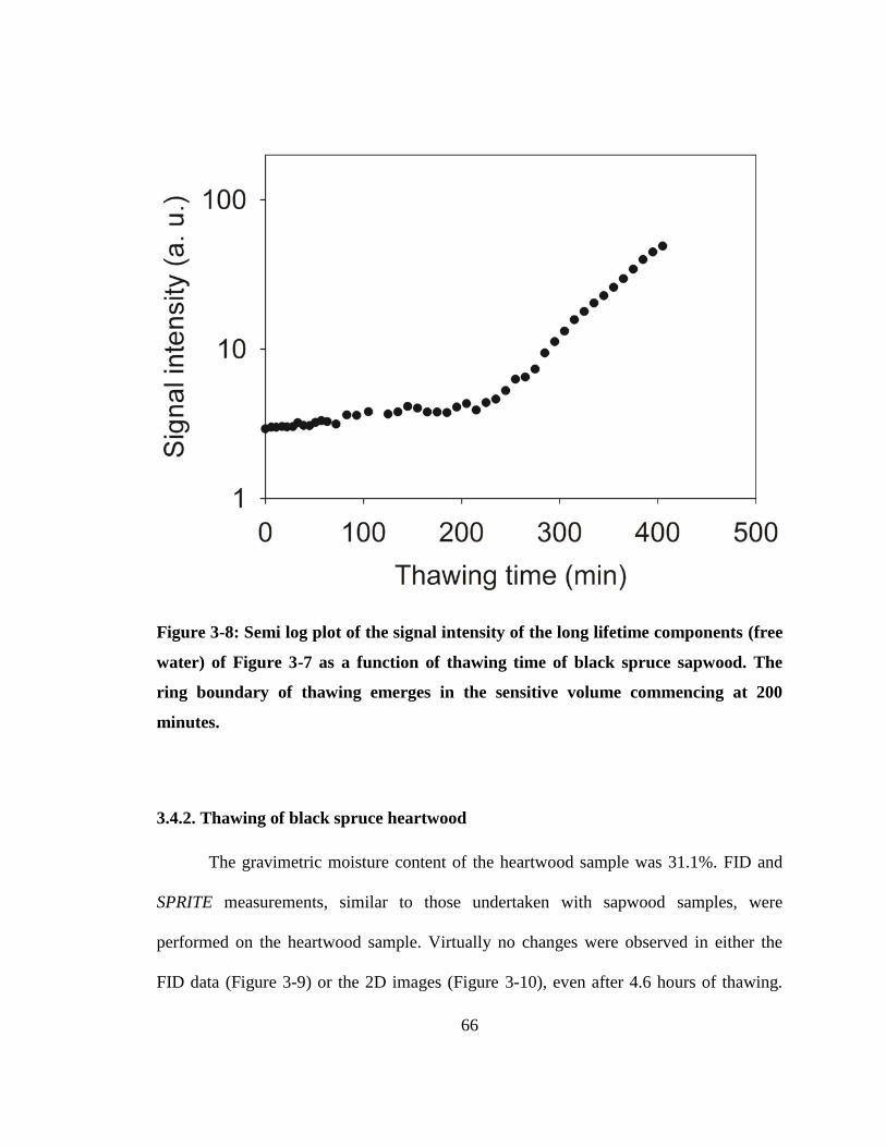
66

Figure 3-8: Semi log plot of the signal intensity of the long lifetime components (free

water) of Figure 3-7 as a function of thawing time of black spruce sapwood. The

ring boundary of thawing emerges in the sensitive volume commencing at 200

minutes.

3.4.2. Thawing of black spruce heartwood

The gravimetric moisture content of the heartwood sample was 31.1%. FID and

SPRITE measurements, similar to those undertaken with sapwood samples, were

performed on the heartwood sample. Virtually no changes were observed in either the

FID data (Figure 3-9) or the 2D images (Figure 3-10), even after 4.6 hours of thawing.

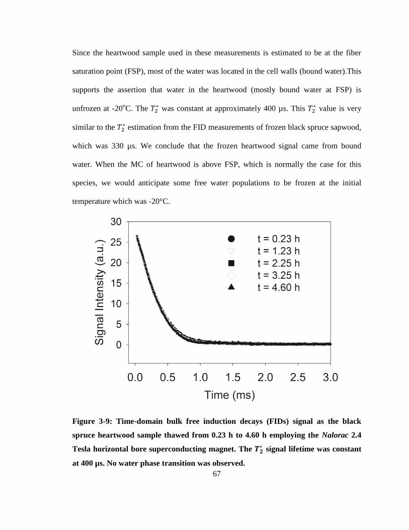
67

Since the heartwood sample used in these measurements is estimated to be at the fiber

saturation point (FSP), most of the water was located in the cell walls (bound water).This

supports the assertion that water in the heartwood (mostly bound water at FSP) is

unfrozen at -20oC. The 𝑇2

∗ was constant at approximately 400 µs. This 𝑇2∗ value is very

similar to the 𝑇2∗ estimation from the FID measurements of frozen black spruce sapwood,

which was 330 µs. We conclude that the frozen heartwood signal came from bound

water. When the MC of heartwood is above FSP, which is normally the case for this

species, we would anticipate some free water populations to be frozen at the initial

temperature which was -20°C.

Figure 3-9: Time-domain bulk free induction decays (FIDs) signal as the black

spruce heartwood sample thawed from 0.23 h to 4.60 h employing the Nalorac 2.4

Tesla horizontal bore superconducting magnet. The 𝑻𝟐∗ signal lifetime was constant

at 400 µs. No water phase transition was observed.

68

Figure 3-10: SPRITE MRI images of a black spruce heartwood sample in the

transverse (left) and tangential (right) planes as a function of thawing time. No

changes were observed even after 4.6 hours of warming. The heartwood sample was

at the fiber saturation point, therefore, most of the water was in the cell walls.

Bound water was not frozen at measurement conditions.

69

3.4.3. Freezing of black spruce sample

Sapwood was employed for the freezing study to permit observation of both

bound and free water. We did not employ heartwood sample in these measurements

because the heartwood sample was estimated to be at FSP. The gravimetric moisture

content of the sapwood sample employed was 110%. Figure 3-11 shows the bulk FIDs as

a function of time for different temperatures as the black spruce sapwood sample froze.

The bulk FID signal decreases as the temperature goes from -1°C to -100°C.Signal from

frozen water is undetectable with our MR apparatus.

Figure 3-11: Time-domain bulk free induction decays (FIDs) as a function of time

for different temperatures as the black spruce sapwood sample froze. Signal

decreases with temperature as water underwent a phase change. The time between

points on the FID was 5 µs.

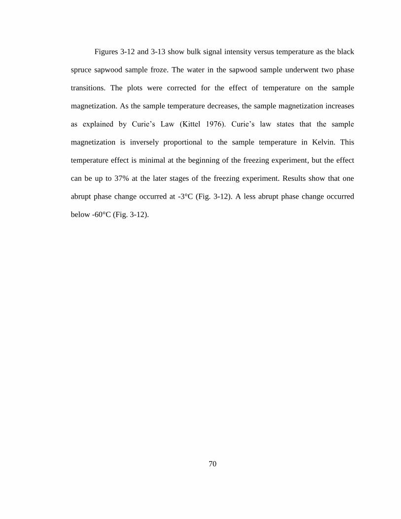
70

Figures 3-12 and 3-13 show bulk signal intensity versus temperature as the black

spruce sapwood sample froze. The water in the sapwood sample underwent two phase

transitions. The plots were corrected for the effect of temperature on the sample

magnetization. As the sample temperature decreases, the sample magnetization increases

as explained by Curie’s Law (Kittel 1976). Curie’s law states that the sample

magnetization is inversely proportional to the sample temperature in Kelvin. This

temperature effect is minimal at the beginning of the freezing experiment, but the effect

can be up to 37% at the later stages of the freezing experiment. Results show that one

abrupt phase change occurred at -3°C (Fig. 3-12). A less abrupt phase change occurred

below -60°C (Fig. 3-12).

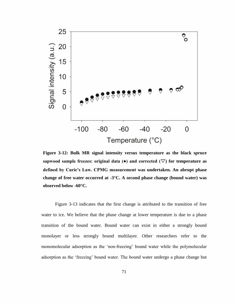
71

Figure 3-12: Bulk MR signal intensity versus temperature as the black spruce

sapwood sample freezes: original data (●) and corrected (▽) for temperature as

defined by Curie’s Law. CPMG measurement was undertaken. An abrupt phase

change of free water occurred at -3°C. A second phase change (bound water) was

observed below -60°C.

Figure 3-13 indicates that the first change is attributed to the transition of free

water to ice. We believe that the phase change at lower temperature is due to a phase

transition of the bound water. Bound water can exist in either a strongly bound

monolayer or less strongly bound multilayer. Other researchers refer to the

monomolecular adsorption as the ‘non-freezing’ bound water while the polymolecular

adsorption as the ‘freezing’ bound water. The bound water undergo a phase change but

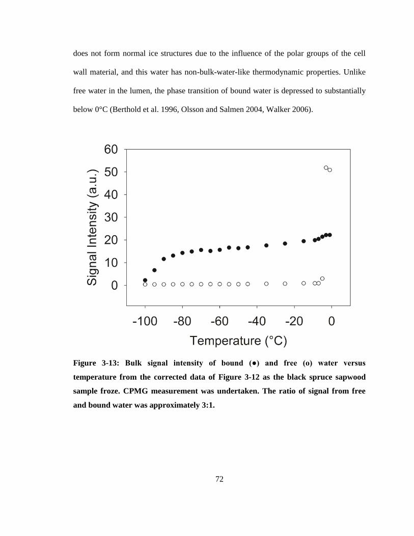
72

does not form normal ice structures due to the influence of the polar groups of the cell

wall material, and this water has non-bulk-water-like thermodynamic properties. Unlike

free water in the lumen, the phase transition of bound water is depressed to substantially

below 0°C (Berthold et al. 1996, Olsson and Salmen 2004, Walker 2006).

Figure 3-13: Bulk signal intensity of bound (●) and free (o) water versus

temperature from the corrected data of Figure 3-12 as the black spruce sapwood

sample froze. CPMG measurement was undertaken. The ratio of signal from free

and bound water was approximately 3:1.

73

The signal intensity before the first phase transition (where free water freezes) is 3

times higher than the signal intensity after the first phase transition. This is consistent

with the ratio of bound and free water in this sample, which was measured to be 3:1 using

the FID measurements (Figure 3-3).

Figures 3-13 and 3-14 show the signal intensities and T2 values of free and bound

water as a function of temperature from the data in Figure 3-12. The signal intensity and

T2 were determined employing CPMG measurements. Figures 3-13 and 3-14 suggest that

the abrupt transition in free water occurred at -3°C. Signal from free water is no longer

observable below this temperature. The T2 of bound water is much shorter than the T2 of

free water (Riggins et al. 1979 and Araujo et al. 1992). There was a slight decrease of T2

from bound water as temperature decreased. The phase transition of bound water

occurred over a wider temperature range than the abrupt transition of the free water.

Movement of bound water is restricted as it is confined in the cell wall through hydrogen

bonds.

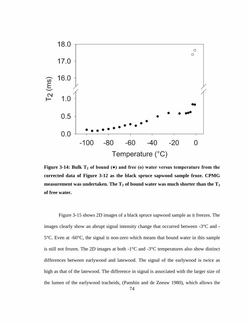
74

Figure 3-14: Bulk T2 of bound (●) and free (o) water versus temperature from the

corrected data of Figure 3-12 as the black spruce sapwood sample froze. CPMG

measurement was undertaken. The T2 of bound water was much shorter than the T2

of free water.

Figure 3-15 shows 2D images of a black spruce sapwood sample as it freezes. The

images clearly show an abrupt signal intensity change that occurred between -3°C and -

5°C. Even at -60°C, the signal is non-zero which means that bound water in this sample

is still not frozen. The 2D images at both -1°C and -3°C temperatures also show distinct

differences between earlywood and latewood. The signal of the earlywood is twice as

high as that of the latewood. The difference in signal is associated with the larger size of

the lumen of the earlywood tracheids, (Panshin and de Zeeuw 1980), which allows the

75

earlywood to accommodate more free water. This result is consistent with the findings of

other studies of moisture content in earlywood and latewood of green coniferous species.

The moisture content in the early sapwood is much higher than in latewood. The

coniferous species studied include Pinus radiata D. Don. (Harris 1961, Kininmonth and

Whitehouse 1991) and Pseudotsuga menziesii Franco (Harris 1961 and Raczkowski et al.

2000).

The SPRITE MRI measurements employed determined the phase transition of

bound water which is challenging for other techniques, such as calorimetry based

methods.

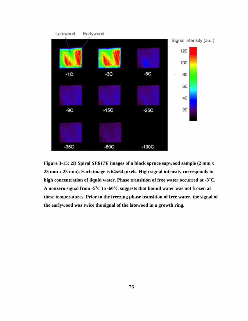
76

Figure 3-15: 2D Spiral SPRITE images of a black spruce sapwood sample (2 mm x

25 mm x 25 mm). Each image is 64x64 pixels. High signal intensity corresponds to

high concentration of liquid water. Phase transition of free water occurred at -3oC.

A nonzero signal from -5oC to -60

oC suggests that bound water was not frozen at

these temperatures. Prior to the freezing phase transition of free water, the signal of

the earlywood was twice the signal of the latewood in a growth ring.

77

3.5 Conclusions

The use of a unilateral magnetic resonance instrument and the SPRITE MRI

measurement in a series of thawing and freezing experiments established the possibility

of studying water phase transitions in frozen wood samples. An abrupt phase transition of

free water was observed at -3°C. A more diffuse phase transition occurred below -60°C

which was attributed to a phase change of bound water.

The unilateral magnetic resonance instrument and SPRITE MRI measurement

employed allowed measurements of relative quantities of bound and free water in wood.

None of the MR and MRI measurements undertaken are able to measure frozen water

directly. We may infer the quantity of frozen water by temperature dependent

measurements of samples which are initially unfrozen. However, direct MR and MRI

measurements of frozen samples do not permit an estimation of the amount of frozen

water. This is true for small laboratory samples and log samples in the field.

In addition, the results demonstrate the use of unilateral magnetic resonance as a

powerful tool, which is portable, to monitor water quantity and quantify bound and free

water in green log samples. The unilateral magnet employed in this study is currently

being evaluated in measuring moisture content of drying logs with a through bark

measurement.

78

3.6 References

Almeida G, Gagne S, Hernandez RE (2007) A NMR study of water distribution in

hardwoods at several equilibrium moisture contents. Wood Sci Technol

41(4):293-307.

Araujo CD, Mackay AL, Hailey JRT, Whittall KP, Le H (1992) Proton magnetic

resonance techniques for characterization of water in wood: application to white

spruce. Wood Sci Technol 26 (2):101-113.

Balcom BJ, MacGregor RP, Beyea SD, Green DP, Armstrong RL, Bremner TW (1996)

Single point ramped imaging with T1 enhancement (SPRITE). J Magn Reson

A123(1):131-134.

Berthold J, Rinaudo M, Salmén L (1996) Association of water to polar groups;

estimations by an adsorption model for lingo-cellulosic materials. Colloids and

Surfaces A: physiochemical and engineering aspects (112):117-129.

Carslaw HS, Jaeger JC (1959) Conduction of heat in solids. 2nd

Ed. Oxford University

Press, New York. 510 pp.

Filbotte S, Menon RS, MacKay AL, Hailey JRT (1990) Proton magnetic resonance of

western red cedar. Wood Fiber Sci 22(4):362-376.

FPL (2010) Wood handbook – Wood as an engineering material. Gen Tech Rep FPL-

GTR-190. USDA For Serv Forest Products Laboratory, Madison, WI. 508 pp.

Gazdzizski S, Hartley ID, and Peemoeller H (2000) Freezing in trembling aspen (Populus

Tremuloides Michx.) by 1H NMR relaxometry. Molecular Physics Reports

29:144-146.

Hall LD, Rajanayagam V, Stewart WA, Steiner PR (1986). Magnetic resonance imaging

of wood. Can J Forest Res 16(2):423-426.

Halse M, Goodyear DJ, MacMillan B, Szomolanyi P, Matheson D, Balcom BJ (2003)

Centric scan SPRITE magnetic resonance imaging. J Magn Reson 165(2):219-

229.

Hameury S, Sterley M (2006) Magnetic resonance imaging of moisture distribution in

Pinus sylvestris L. exposed to daily indoor relative humidity fluctuations. Wood

Mater Sci Eng, 1:116-126.

Harris JM (1961) Water conduction in the stems of certain conifers. Nature

189(4765):678-679.

79




Karenlampi PP, Tynjala P, Strom P (2005) Phase transformations of wood cell wall

water. J Wood Sci 51(2):118-123.

Kininmonth JA, Whitehouse LJ (1991) Properties and uses of New Zealand radiate pine.

Vol. 1. Wood properties. New Zealand Forest Research Institute, Jan Bryce

Printers Ltd., Rotorna:74-76.

Kittel C (1976) Introduction to solid state physics. 5th

edition. John Wiley and sons, Inc.,

New York. p. 440.

Liang, Z-P, Lauterbur PC (2000) Principle of Magnetic Resonance Imaging – A signal

processing perspective. The Institute of Electrical and Electronics Engineers, Inc.,

New York. pp. 57-76.

MacMillan B, Schneider MH, Sharp AR, Balcom BJ (2002) Magnetic resonance imaging

of water concentration in low moisture content wood. Wood Fiber Sci 34(2):276-

286.

MacMillan B, Veliyulin E, Lamason C, Balcom BJ (2011) Quantitative magnetic

resonance measurements of low moisture content wood. Can J Forest Re 41:2158-

2162.

Marble AE, Mastikhin IV, Colpitts BG, Balcom BJ (2007) A compact permanent magnet

array with a remote homogenous field. J Magn Reson 186 (1):100-104.

Meder R, Franich RA, Callaghan PT (1999) 11B magnetic resonance imaging and MAS

spectroscopy of trimethylborate-treated radiate pine wood. Solid State Nucl Magn

Reson 15 (1):69-72.

Menon RS, MacKay AL, Hailey JRT, Bloom M, Burgess AE, Swanson JS (1987) An

NMR determination of the physiological water distribution in wood during

drying. J Appl Polym Sci 23(11):3147-3154.

Merchant MV (1957) A study of water-swollen cellulose fibres which have been liquid-

exchanged and dried from hydrocarbons. Tappi 40 (9):771-781.

Nyström J, Dahlquist E (2004) Methods for Determination of moisture content in

woodchips for power plants - a Review. Fuel (83):773–779.

Olsson AM, Salmén L (2004) The association of water to cellulose and hemicellulose in

paper examined by FTIR spectroscopy. Carbohydrate Research (339):813-818.

80

Panshin AJ, de Zeeuw C (1980) Textbook of wood technology. 4th

Ed. McGraw-Hill

Publishing Company, New York. pp. 722.

Prado PJ, Balcom BJ, Beyea SD, Bremner TW, Armstrong RL, Grattan-Bellew PE

(1998) Concrete freeze/thaw as studied by magnetic resonance imaging. Cement

Concrete Res 28 (2):261-270.

Quick JJ, Hailey JRT, MacKay AL (1990) Radial moisture profiles of cedar sapwood

during drying: A proton magnetic resonance study. Wood Fiber Sci 22(4):404-

412.

Raczkowski J, Olek W, Guzenda R (200) Moisture evaporation rates from sapwood

andheartwood samples of Douglas Fir (Pseudotsuga menziesii Franco) green

wood. Holz Roh – Werkst. 58:247-252.

Siau JF (1971) Flow in Wood. 1st Ed. Syracuse University Press, Syracuse, New York.

pp. 131.

Skaar C (1988) Wood-water relations. Springer-Verlag, New York. 283 pp.

Sparks JP, Campbell GS, Black RA (2000). Liquid water content of wood tissue at

temperatures below 0oC. Can J Forest Res 30 (4):624-630.

Stenstrom S, Bonazzi C, Foucat L (2009) Magnetic resonance imaging for determination

of moisture profiles and drying curves. In Modern drying technology. Vol. 2.

Experimental techniques. Edited by E. Tsotsas and A. S. Mujumdar. Wiley-VCH,

Weinheim, Germany. pp. 91-142.

Steinhagen HP (1977) Thermal conductive properties of wood, green or dry, from -40° to

+100°C: A literature review. Gen Tech Rep FPL-9. USDA For Serv Forest

Products Laboratory, Madison, WI.

Szomolanyi P, Goodyear D, Balcom BJ, Matheson D (2001) SPIRAL-SPRITE: a rapid

single point MRI technique for application to porous media. Magn Reson Imaging

19 (3-4):423-428.

Tarkow H (1971) On a reinterpretation of anomalous moisture adsorption isobars below

0°C. Tappi 54(4):593.

Thygesen LG, Engelund ET, and Hoffmeyer P (2010) Water sorption in wood and

modified wood at high values of relative humidity – Part 1: results for untreated,

acetylated, and furfurylated Norway spruce. Holzforschung 64:315-323.

81

Van Dyk H, Rice RW (2005) Ultrasonic wave velocity as a moisture indicator in frozen

and unfrozen lumber. Forest Prod J 55(6):68-72.

Wang PC, Chang SJ (1986) Nuclear magnetic resonance imaging of wood. Wood Fiber

Sci 18 (2):308-314.

Zelinka SL, Lambrecht MJ, Glass SV, Wiedenhoeft AC, Yelle DJ (2012) Examination of

water phase transitions in Loblolly pine and cell wall components by differential

scanning calorimetry. Thermochim Acta 533:39-45.

82

Chapter 4 – Water content measurement in black spruce and aspen

sapwood with benchtop and portable magnetic resonance devices

In the previous chapter, it was demonstrated that UMR works well detecting

signal from water in thawed wood sample. This chapter discusses how time-domain MR

measurements easily distinguish water in different environments in wood according to

the spin-spin relaxation time and provide quantitative information on water content. A

portable UMR device was employed to measure water content in black spruce (Picea

mariana Mill.) and aspen (Populus tremuloides Michx.). A benchtop MR device which

has a homogenous magnetic field was employed to compare the results of the UMR

device. The aspen sample employed for the measurement was not fully saturated however

the sample was still above FSP.

This chapter is largely based on the paper “Water content measurement in black

spruce and aspen sapwood with benchtop and portable magnetic resonance devices”

published in the Wood Material Science and Engineering Journal (Lamason et al. 2015).

The format of references in this chapter follows that of the original article.

4.1 Introduction

Wood is a hygroscopic and anisotropic material whose properties are deeply

influenced by the presence of water. The physical properties of wood are dependent on its

chemical composition and lignocellulosic structures, as well as the moisture content.

Measurements of moisture content (MC) of wood are therefore of considerable

83

importance. Water in wood exists in two general states. By convention, the first is called

free water (or absorbed water) and corresponds to the water located in the lumen and

other void spaces. The second is called bound water (or adsorbed water) and corresponds

to the water in the cell wall. Water in the cell walls is motionally restricted compared to

water in the lumen. The condition at which the cell wall is saturated with water, with no

water in the cell lumen, is termed the fiber saturation point (FSP). This occurs at around

30% MC for most species (Stamm 1964, Walker 2006). The loss of cell wall water is

usually studied separately from the loss of lumen water in wood during drying, because it

is difficult to identify both water states simultaneously with traditional measurement

methods.

Water in wood has been extensively studied by numerous experimental methods.

One of those methods is magnetic resonance (see the review of Engelund et al. 2013).

Magnetic resonance (MR) and magnetic resonance imaging (MRI) techniques have been

employed to estimate MC in wood pellets (Nyström and Dahlquist 2004), in drying

studies (Sharp et al. 1978, Hall et al. 1986, Menon et al. 1987, Quick et al. 1990, Araujo

et al. 1992, Hartley et al. 1994, MacMillan et al. 2002, 2011, Hameury et al. 2006,

Almeida et al. 2007, Stenstrom et al. 2009) and in wood freeze/thaw studies (Lamason et

al. 2014). Most MRI studies consider relatively wet wood because conventional MRI

techniques are not quantitative at low moisture contents.

There are relatively few studies in the literature which employ portable unilateral

MR sensors. Casieri et al. (2004) employed mobile MR as a non-destructive and non-

invasive tool for water content analysis and moisture fraction determination in wood.

Senni et al. (2009) employed a portable MR sensor for in situ non-invasive determination

84

of moisture content of wooden works of art and painted wood. Portable unilateral MR

was employed by Dvinskikh et al. (2011) to study moisture content profiles and uptake

kinetics in wood materials. Pourmand et al. (2011) evaluated the moisture protective

properties of wood coating by a portable MR sensor. Most of the sensors employed by

these researchers have a maximum depth of penetration of 3-5 mm. In the current work, a

portable unilateral MR sensor with a maximum depth of penetration of 13 mm is

evaluated and applied in wood moisture measurements. This permits measurements

beyond the surface and near surface, and beyond most bark layers and cambium, in log

samples. In wood materials, the layer below the bark and cambium is the sapwood.The

hydrogen nuclei in a water molecule, H2O, consist of a single proton. The proton has spin

angular momentum and thereby a magnetic moment. The magnetic moments are excited

by radio frequency (RF) magnetic fields and then detected by induction in the RF probe.

The strength of the MR signal is proportional to the number of 1H nuclei in the sample

volume, and thus to the water content of the scanned sample. The MR phenomenon

occurs at a specific frequency, the resonance frequency. According to the Larmor

equation, the resonance frequency is linearly dependent on both the strength of the

magnetic field and a nuclear property known as the gyromagnetic ratio (Liang and

Lauterbur 2000).

𝜔 = γB0 (Equation 4-1)

where 𝜔 is the resonance frequency also known as the Larmor frequency (MHz),

γ is the gyromagnetic ratio (42.58 MHz/Tesla for 1H), and B0 is the static magnetic field

strength (Tesla).

85

One important advantage of magnetic resonance is the ability to distinguish cell

wall and lumen water in one measurement. Interactions between spins are influenced by

the local magnetic fields, which are functions of the spin environment. Differences in the

environment produce a different MR spin-spin relaxation time (T2) because T2 is a

function of the molecular mobility (Abragam 1961). Liquids typically have longer T2

than solids. In wood materials, bound water has short T2 values, up to a few ms, whereas

free water has T2 values from tens to 100s of ms (Menon et al 1987).

Both the cell wall and the lumen water exist in two different sub-environments.

According to the Brunauer, Emmett and Teller (BET) theory (Brunauer, Emmett and

Teller 1938), the cell wall water has a monolayer of strongly adsorbed water molecules

and multiple layers of adsorbed water. The moisture needed to form a monomolecular

surface layer within the non-crystalline regions of the cell wall was calculated to

correspond to a moisture content of about 5% (Stamm 1964, Walker 2006). The BET

equation that corresponds to a sigmoidal adsorption curve allows calculation of the

average number of molecular layers of water at fiber saturation. Stamm (1964) reported

6.5 layers for Sitka spruce (Picea sitchensis (Bong) Carr.) and 7.5 layers of sugar maple

(Acer saccharum Marshall). Riggin et al. (1979) observe a single T2 for the bound water

signal component. This is presumably due to rapid exchange of the monolayer and

multilayer bound water.

For porous media such as wood, where free water is present in lumen, void

spaces, or trapped in micro pores, the spin-spin relaxation rate (1

𝑇2) is expressed as the

weighted sum of the surface relaxation rate and the bulk water relaxation rate (Wong

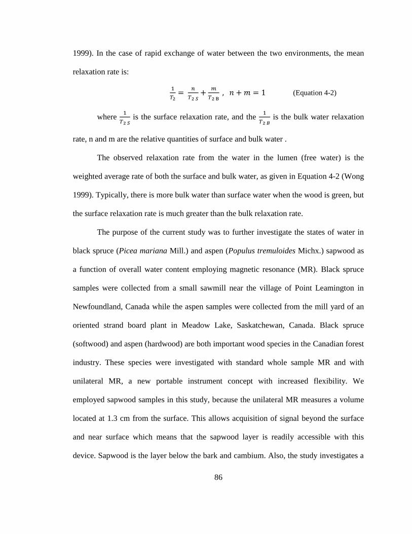
86

1999). In the case of rapid exchange of water between the two environments, the mean

relaxation rate is:

1

𝑇2=

𝑛

𝑇2 𝑆+

𝑚

𝑇2 B , 𝑛 + 𝑚 = 1 (Equation 4-2)

where 1


1

𝑇2 𝐵 is the bulk water relaxation

rate, n and m are the relative quantities of surface and bulk water .

The observed relaxation rate from the water in the lumen (free water) is the

weighted average rate of both the surface and bulk water, as given in Equation 4-2 (Wong

1999). Typically, there is more bulk water than surface water when the wood is green, but

the surface relaxation rate is much greater than the bulk relaxation rate.

The purpose of the current study was to further investigate the states of water in

black spruce (Picea mariana Mill.) and aspen (Populus tremuloides Michx.) sapwood as

a function of overall water content employing magnetic resonance (MR). Black spruce

samples were collected from a small sawmill near the village of Point Leamington in

Newfoundland, Canada while the aspen samples were collected from the mill yard of an

oriented strand board plant in Meadow Lake, Saskatchewan, Canada. Black spruce

(softwood) and aspen (hardwood) are both important wood species in the Canadian forest

industry. These species were investigated with standard whole sample MR and with

unilateral MR, a new portable instrument concept with increased flexibility. We

employed sapwood samples in this study, because the unilateral MR measures a volume

located at 1.3 cm from the surface. This allows acquisition of signal beyond the surface

and near surface which means that the sapwood layer is readily accessible with this

device. Sapwood is the layer below the bark and cambium. Also, the study investigates a

87

full range of MC values (from almost 0% to 140% dry basis). This is the first time that

our unilateral magnetic resonance device has been employed to quantify water in wood.


Whole sample magnetic resonance (MR) measurement employed a 10 MHz

Bruker Minispec mq10 NMR Analyzer (Rheinstetten, Germany) (Figure 4-1). This

instrument utilized a cylindrical wood sample of approximately 8-mm diameter and 20-

mm length (longitudinal direction). The cylindrical sample was cut from the sapwood of

freshly harvested black spruce and aspen disks. The instrument measures the spin-spin

relaxation time and signal amplitude using the Carr Purcell Meiboom Gill (CPMG)

measurement with an echo time of 0.06 ms for 512 echoes. The CPMG measurement is a

spin echo measurement consisting of a 90o radio frequency (RF) pulse followed by an

echo train induced by successive 180o RF pulses. The 90° pulse length was 2.9 µs. The

overall acquisition time was approximately 1 min.

88

Figure 4-1: Photograph of the 10 MHz Bruker Minispec instrument employed in this

study. This instrument employed 10 mm NMR tubes with an inside diameter of

approximately 8 mm. The wood plug is inside the NMR tube which is inserted

vertically as shown. The black surface behind the sample is not part of the

instrument. It is there solely to highlight the sample.

A 30 mm x 40 mm x 40 mm block of sapwood was cut adjacent to the cylindrical

sample employed in the 10 MHz Bruker Minispec measurements. The MC of this block

was measured with a unilateral MR device that was designed and developed at the UNB

MRI Centre. The device is a lightweight 3 magnet array which features open access and

is portable (Marble et. al. 2007). Figure 4-2 is a photograph of the unilateral magnet

along with the RF coil. Figure 4-3 plots the magnetic field along the central vertical line

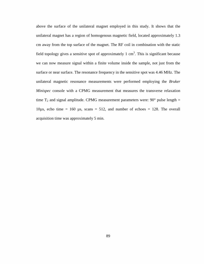
89

above the surface of the unilateral magnet employed in this study. It shows that the

unilateral magnet has a region of homogenous magnetic field, located approximately 1.3

cm away from the top surface of the magnet. The RF coil in combination with the static

field topology gives a sensitive spot of approximately 1 cm3. This is significant because

we can now measure signal within a finite volume inside the sample, not just from the

surface or near surface. The resonance frequency in the sensitive spot was 4.46 MHz. The

unilateral magnetic resonance measurements were performed employing the Bruker

Minispec console with a CPMG measurement that measures the transverse relaxation

time T2 and signal amplitude. CPMG measurement parameters were: 90° pulse length =

10µs, echo time = 160 µs, scans = 512, and number of echoes = 128. The overall

acquisition time was approximately 5 min.

90

Figure 4-2: Photograph of a unilateral magnet device employed in this study. The




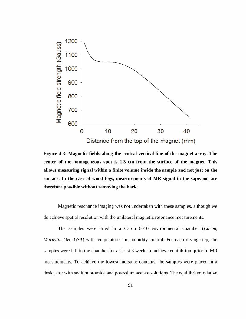
91

Figure 4-3: Magnetic fields along the central vertical line of the magnet array. The


allows measuring signal within a finite volume inside the sample and not just on the


therefore possible without removing the bark.

Magnetic resonance imaging was not undertaken with these samples, although we

do achieve spatial resolution with the unilateral magnetic resonance measurements.

The samples were dried in a Caron 6010 environmental chamber (Caron,

Marietta, OH, USA) with temperature and humidity control. For each drying step, the

samples were left in the chamber for at least 3 weeks to achieve equilibrium prior to MR

measurements. To achieve the lowest moisture contents, the samples were placed in a

desiccator with sodium bromide and potassium acetate solutions. The equilibrium relative

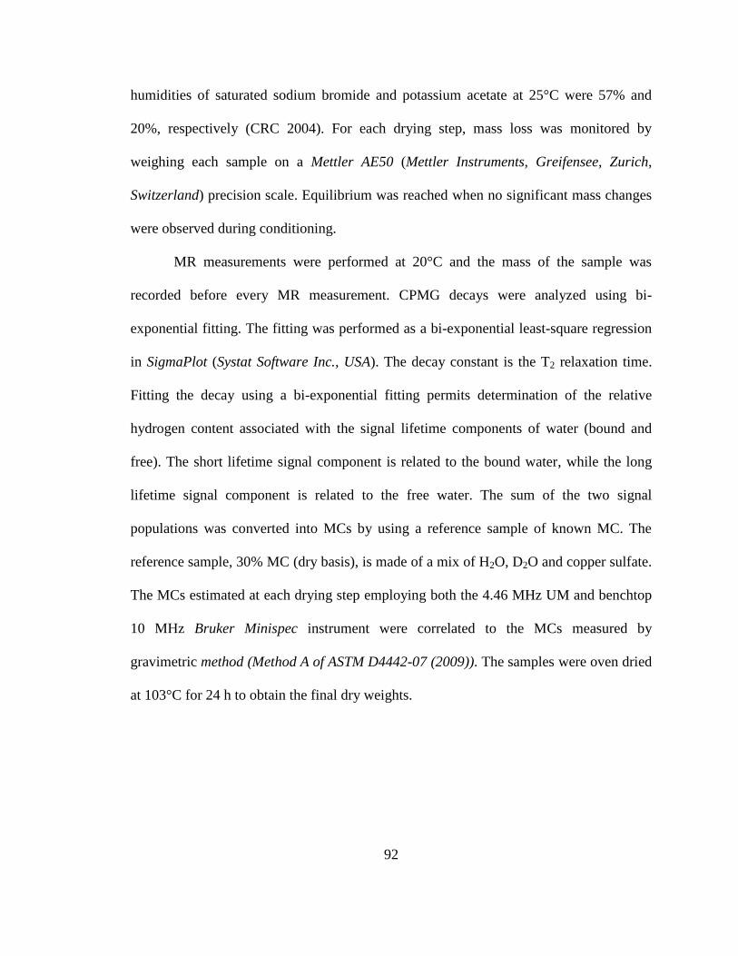
92

humidities of saturated sodium bromide and potassium acetate at 25°C were 57% and

20%, respectively (CRC 2004). For each drying step, mass loss was monitored by

weighing each sample on a Mettler AE50 (Mettler Instruments, Greifensee, Zurich,

Switzerland) precision scale. Equilibrium was reached when no significant mass changes

were observed during conditioning.

MR measurements were performed at 20°C and the mass of the sample was

recorded before every MR measurement. CPMG decays were analyzed using bi-

exponential fitting. The fitting was performed as a bi-exponential least-square regression

in SigmaPlot (Systat Software Inc., USA). The decay constant is the T2 relaxation time.

Fitting the decay using a bi-exponential fitting permits determination of the relative

hydrogen content associated with the signal lifetime components of water (bound and

free). The short lifetime signal component is related to the bound water, while the long

lifetime signal component is related to the free water. The sum of the two signal

populations was converted into MCs by using a reference sample of known MC. The

reference sample, 30% MC (dry basis), is made of a mix of H2O, D2O and copper sulfate.

The MCs estimated at each drying step employing both the 4.46 MHz UM and benchtop

10 MHz Bruker Minispec instrument were correlated to the MCs measured by

gravimetric method (Method A of ASTM D4442-07 (2009)). The samples were oven dried

at 103°C for 24 h to obtain the final dry weights.

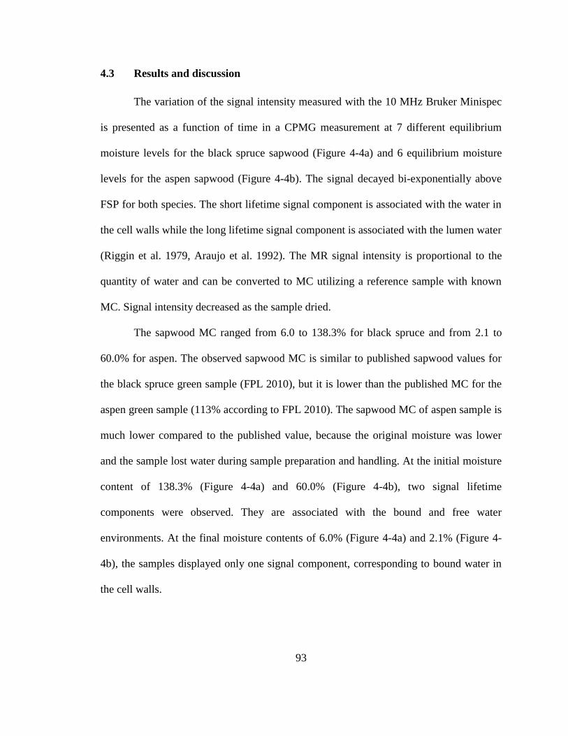
93


The variation of the signal intensity measured with the 10 MHz Bruker Minispec

is presented as a function of time in a CPMG measurement at 7 different equilibrium

moisture levels for the black spruce sapwood (Figure 4-4a) and 6 equilibrium moisture

levels for the aspen sapwood (Figure 4-4b). The signal decayed bi-exponentially above

FSP for both species. The short lifetime signal component is associated with the water in

the cell walls while the long lifetime signal component is associated with the lumen water

(Riggin et al. 1979, Araujo et al. 1992). The MR signal intensity is proportional to the

quantity of water and can be converted to MC utilizing a reference sample with known

MC. Signal intensity decreased as the sample dried.

The sapwood MC ranged from 6.0 to 138.3% for black spruce and from 2.1 to

60.0% for aspen. The observed sapwood MC is similar to published sapwood values for

the black spruce green sample (FPL 2010), but it is lower than the published MC for the

aspen green sample (113% according to FPL 2010). The sapwood MC of aspen sample is

much lower compared to the published value, because the original moisture was lower

and the sample lost water during sample preparation and handling. At the initial moisture

content of 138.3% (Figure 4-4a) and 60.0% (Figure 4-4b), two signal lifetime

components were observed. They are associated with the bound and free water

environments. At the final moisture contents of 6.0% (Figure 4-4a) and 2.1% (Figure 4-

4b), the samples displayed only one signal component, corresponding to bound water in

the cell walls.

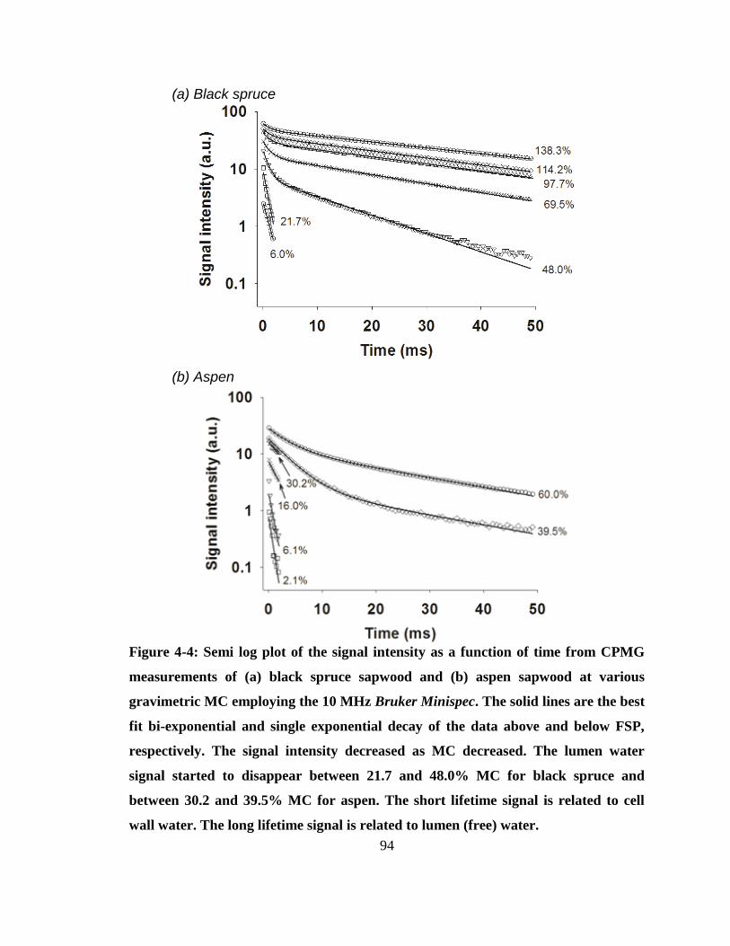
94

(a) Black spruce

(b) Aspen



gravimetric MC employing the 10 MHz Bruker Minispec. The solid lines are the best

fit bi-exponential and single exponential decay of the data above and below FSP,

respectively. The signal intensity decreased as MC decreased. The lumen water

signal started to disappear between 21.7 and 48.0% MC for black spruce and

between 30.2 and 39.5% MC for aspen. The short lifetime signal is related to cell

wall water. The long lifetime signal is related to lumen (free) water.

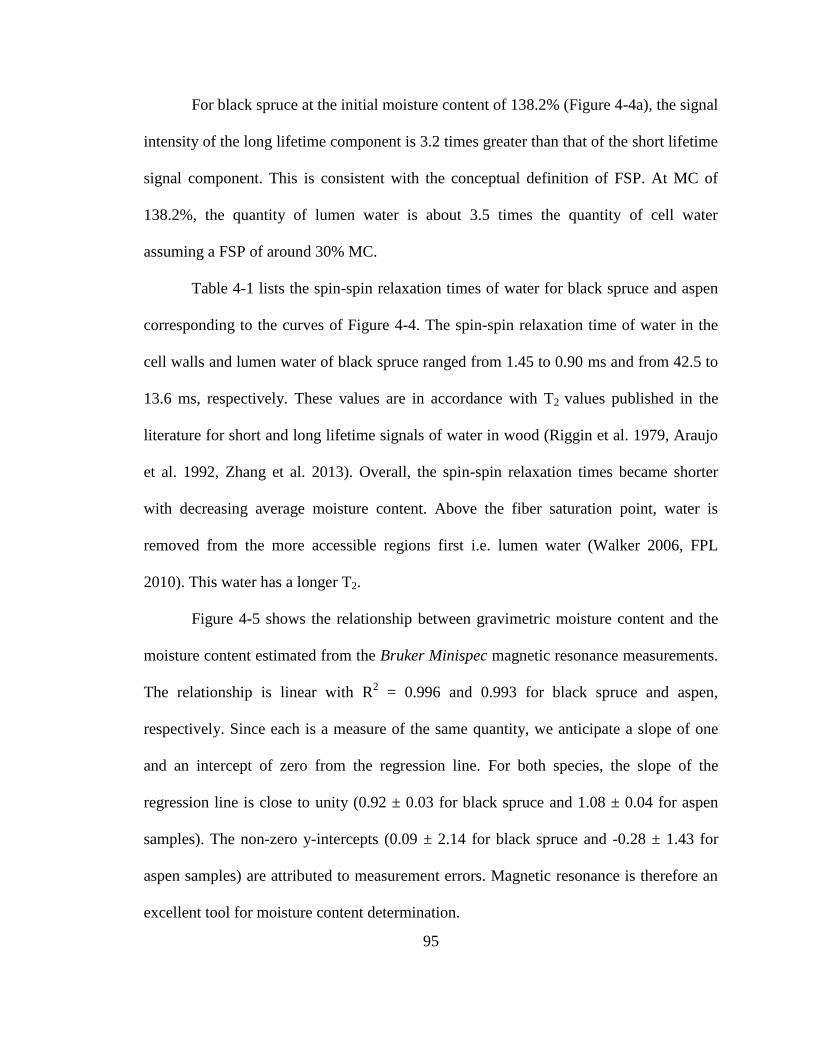
95

For black spruce at the initial moisture content of 138.2% (Figure 4-4a), the signal

intensity of the long lifetime component is 3.2 times greater than that of the short lifetime

signal component. This is consistent with the conceptual definition of FSP. At MC of

138.2%, the quantity of lumen water is about 3.5 times the quantity of cell water

assuming a FSP of around 30% MC.

Table 4-1 lists the spin-spin relaxation times of water for black spruce and aspen

corresponding to the curves of Figure 4-4. The spin-spin relaxation time of water in the

cell walls and lumen water of black spruce ranged from 1.45 to 0.90 ms and from 42.5 to

13.6 ms, respectively. These values are in accordance with T2 values published in the

literature for short and long lifetime signals of water in wood (Riggin et al. 1979, Araujo

et al. 1992, Zhang et al. 2013). Overall, the spin-spin relaxation times became shorter

with decreasing average moisture content. Above the fiber saturation point, water is

removed from the more accessible regions first i.e. lumen water (Walker 2006, FPL

2010). This water has a longer T2.

Figure 4-5 shows the relationship between gravimetric moisture content and the

moisture content estimated from the Bruker Minispec magnetic resonance measurements.

The relationship is linear with R2 = 0.996 and 0.993 for black spruce and aspen,

respectively. Since each is a measure of the same quantity, we anticipate a slope of one

and an intercept of zero from the regression line. For both species, the slope of the

regression line is close to unity (0.92 ± 0.03 for black spruce and 1.08 ± 0.04 for aspen

samples). The non-zero y-intercepts (0.09 ± 2.14 for black spruce and -0.28 ± 1.43 for

aspen samples) are attributed to measurement errors. Magnetic resonance is therefore an

excellent tool for moisture content determination.

96

Table 4-1: Spin-spin relaxation times measured with the 10 MHz Bruker Minispec

for black spruce and aspen at different moisture levels. Values for bound (cell wall)

and free (lumen) water at each MC are reported.

Black spruce Aspen

MC (%) Cell wall

water (ms)

Lumen water

(ms)

MC (%) Cell wall

water (ms)

Lumen water

(ms)

138.3

1.45 42.5 60.0 3.9 26.2

114.2

1.29 35.0 39.5 3.9 25.7

97.7

1.24 35.1 30.2 3.9 -

69.5

1.23 27.7 16.0 2.3 -

48.0

1.05 13.6 6.1 0.9 -

21.7

1.10 - 2.1 0.7 -

6.0 0.90 -

97

(a) Black spruce

(b) Aspen

Figure 4-5: Linear relationship between MC determined gravimetrically and by

magnetic resonance employing the 10 MHz Bruker Minispec: (a) black spruce and

(b) aspen.

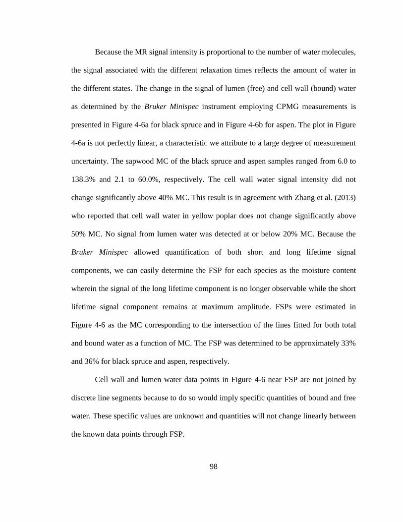
98

Because the MR signal intensity is proportional to the number of water molecules,

the signal associated with the different relaxation times reflects the amount of water in

the different states. The change in the signal of lumen (free) and cell wall (bound) water

as determined by the Bruker Minispec instrument employing CPMG measurements is

presented in Figure 4-6a for black spruce and in Figure 4-6b for aspen. The plot in Figure

4-6a is not perfectly linear, a characteristic we attribute to a large degree of measurement

uncertainty. The sapwood MC of the black spruce and aspen samples ranged from 6.0 to

138.3% and 2.1 to 60.0%, respectively. The cell wall water signal intensity did not

change significantly above 40% MC. This result is in agreement with Zhang et al. (2013)

who reported that cell wall water in yellow poplar does not change significantly above

50% MC. No signal from lumen water was detected at or below 20% MC. Because the

Bruker Minispec allowed quantification of both short and long lifetime signal

components, we can easily determine the FSP for each species as the moisture content

wherein the signal of the long lifetime component is no longer observable while the short

lifetime signal component remains at maximum amplitude. FSPs were estimated in

Figure 4-6 as the MC corresponding to the intersection of the lines fitted for both total

and bound water as a function of MC. The FSP was determined to be approximately 33%

and 36% for black spruce and aspen, respectively.

Cell wall and lumen water data points in Figure 4-6 near FSP are not joined by

discrete line segments because to do so would imply specific quantities of bound and free

water. These specific values are unknown and quantities will not change linearly between

the known data points through FSP.

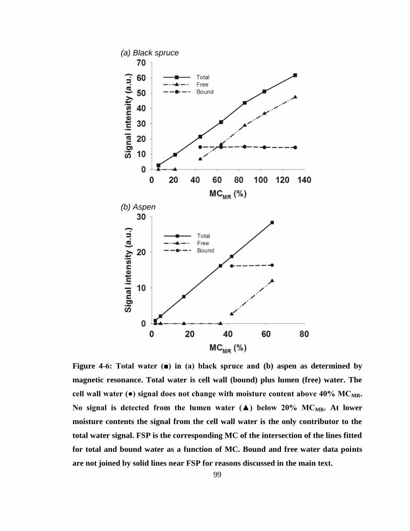
99

(a) Black spruce

(b) Aspen

Figure 4-6: Total water (■) in (a) black spruce and (b) aspen as determined by

magnetic resonance. Total water is cell wall (bound) plus lumen (free) water. The

cell wall water (●) signal does not change with moisture content above 40% MCMR.

No signal is detected from the lumen water (▲) below 20% MCMR. At lower

moisture contents the signal from the cell wall water is the only contributor to the

total water signal. FSP is the corresponding MC of the intersection of the lines fitted

for total and bound water as a function of MC. Bound and free water data points

are not joined by solid lines near FSP for reasons discussed in the main text.

100

Signal intensity measured with the 4.46 MHz unilateral magnet is presented as a

function of time in a CPMG measurement of black spruce sapwood (Figure 4-7a) and

aspen sapwood (Figure 4-7b). The long lifetime signal intensity, both in black spruce and

aspen sapwood, decreased as MC decreased. Although both the short and long lifetime

signals were observed, only the long lifetime signal component can be readily analyzed.

The dead time of the RF probe (̴ 120 µs) employed for this particular unilateral magnet

measurement did not allow quantification of the short lifetime signals. Thereby, the

bound water in the call walls cannot be quantified and only the free water is quantified.

The existence of free water above the fiber saturation point is readily apparent in these

measurements.

The long lifetime signal component was converted to MC (above FSP) by

utilizing a reference sample with known MC. The resulting MCs were then added to the

MC values at FSP determined with the Bruker Minispec measurements. The resulting

total MCs agree well with the MCs obtained by the gravimetric method (Figure 4-8). The

relationship between the gravimetric MC and the MC determined by the unilateral

magnetic resonance were linear with a R2 of 0.995 for black spruce (Fig. 4-8a) and a R

2

of 0.994 for aspen (Fig. 4-8b). Once again we anticipate a slope of one and an intercept of

zero from the regression line since each is a measure of the same quantity. For both

species, the slope of the regression line is close to unity, 0.96 ± 0.03 for black spruce

(Fig. 4-8a) and 1.06 ± 0.05 for aspen samples (Fig. 4-8b). However, the y-intercepts are

non-zero (5.42 ± 2.61 for black spruce and -4.13 ± 3.00 for aspen samples). The absolute

values of the non-zero y-intercepts are greater than the y-intercepts of Figure 4-5. This

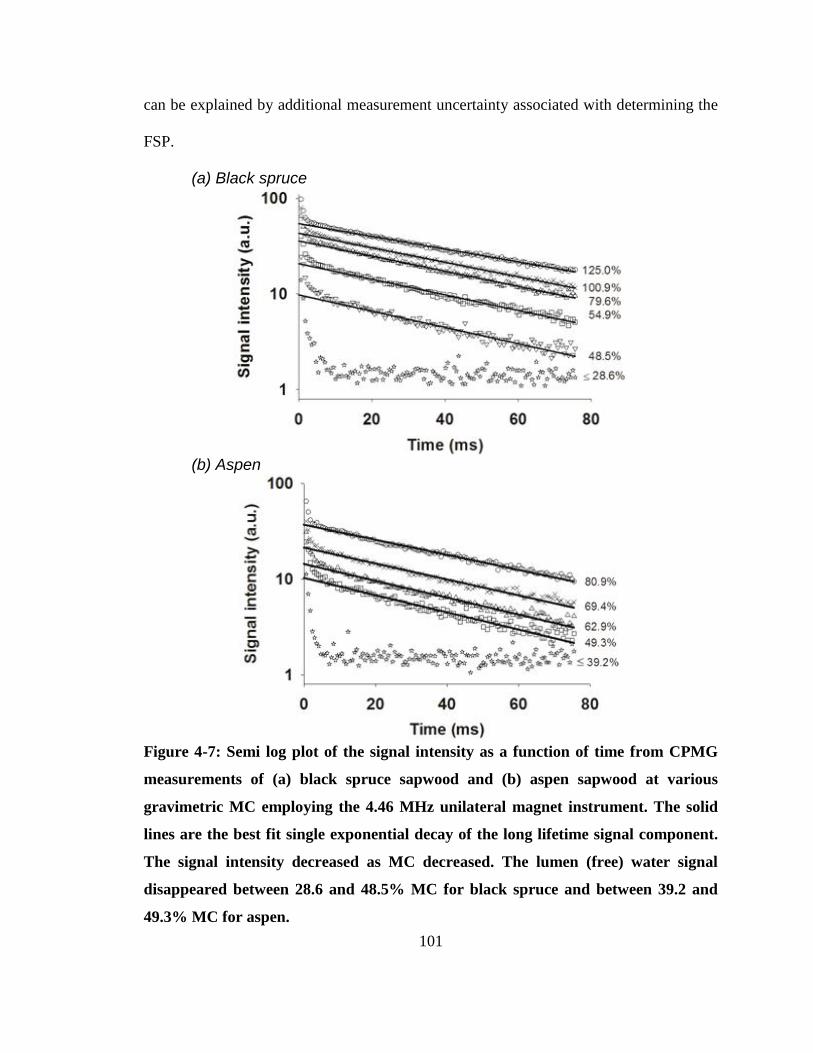
101

can be explained by additional measurement uncertainty associated with determining the

FSP.

(a) Black spruce

(b) Aspen



gravimetric MC employing the 4.46 MHz unilateral magnet instrument. The solid

lines are the best fit single exponential decay of the long lifetime signal component.

The signal intensity decreased as MC decreased. The lumen (free) water signal

disappeared between 28.6 and 48.5% MC for black spruce and between 39.2 and

49.3% MC for aspen.

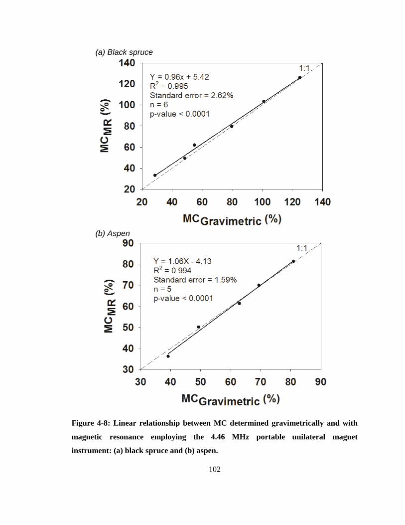
102

(a) Black spruce

(b) Aspen

Figure 4-8: Linear relationship between MC determined gravimetrically and with

magnetic resonance employing the 4.46 MHz portable unilateral magnet

instrument: (a) black spruce and (b) aspen.

103

4.4 Conclusions

It has been shown that magnetic resonance is a powerful tool for distinguishing

water states in wood through measurements of spin-spin relaxation times. Based on this

study, the following conclusions can be made about water states and water behavior in

black spruce and aspen sapwood samples at different moisture contents.

The state of water in wood materials will change with drying. The MR relaxation

times decrease as moisture content decreases. At moisture contents above the fiber

saturation point, water resides in two distinct environments. Free (lumen) water was

removed first while drying above FSP. The amount of bound water does not change

significantly above 40% MC. No signal from free water was observed at or below 20%

MC.

In addition, we demonstrated the use of a portable unilateral magnetic resonance

instrument as a powerful tool in monitoring and estimating moisture content in wood

samples as long as the MC is above FSP. This instrument has the advantage of

portability, permitting moisture content estimations in the field without oven drying. The

estimation of MC employing the unilateral magnet above the FSP agreed well with the

gravimetric MC, particularly at high MCs.

The unilateral magnetic resonance method will allow measurement of water in

samples that are not debarked as it measures a volume located at 1.3 cm below the

surface, which is a significant operational advantage.

104

4.5 References

Abragam, A. (1961). Principles of Nuclear Magnetism. Clarendon Press, Oxford. p 2.

Almeida, G., Gagne, S. and Hernandez, R.E. (2007). A NMR study of water distribution

in hardwoods at several equilibrium moisture contents. Wood Science Technology

41(4):293-307.



10.1520/D4442-07.

Araujo, C.D., Mackay, A.L., Hailey, J.R.T., Whittall, K.P. and Le, H. (1992). Proton

magnetic resonance techniques for characterization of water in wood: application

to white spruce. Wood Science Technology 26 (2):101-113.

Brunauer, S., Emmett, P.H. and Teller, E.J. (1938). Adsorption of gases in multilayers.

Journal of the American Chemical Society 60: 309-319.

Chemical Rubber Company. (2004). Handbook of Chemistry and Physics. 85th

ed. CRC

Press: Boca Raton, FL, 2004-2005; p. 15-36.

Casieri, C., Senni, L., Romagnoli, M., Santamaria, U., De Luca, F. (2004). Determination

of moisture fraction in wood by mobile NMR device. Journal of Magnetic

Resonance 171: 364-372.

Dvinskikh, S. V., Furo, I., Sandberg, D. and Soderstrom, O. (2011). Moisture content

profiles and uptake kinetics in wood cladding materials evaluated by a portable

nuclear magnetic resonance spectrometer. Wood Material Science and

Engineering 6: 119-127.

Engelund, E.T., Thygesen, L.G., Svensson S. and Hill, C. (2013). A critical discussion of

the physics of wood-water interactions. Wood Sci Technol 47:141-161.

Forest Products Laboratory. (2010). Wood handbook - Wood as an engineering material.

Gen Tech Rep FPL-GTR-190. USDA Forest Services, Forest Products

Laboratory, Madison, WI. 509 pp.

Hall, L.D., Rajanayagam, V ., Stewart, W.A. and Steiner, P.R. (1986). Magnetic

resonance imaging of wood. Canadian Journal of Forest Research 16(2): 423-

426.

Hameury, S. and Sterley, M. (2006). Magnetic resonance imaging of moisture

distribution in Pinus sylvestris L. exposed to daily indoor relative humidity

fluctuations. Wood Material Science and Engineering 1:116-126.

105






imaging. Wood and Fiber Sci 46(4):1-14. (also Chapter 3 of this Thesis)

Liang, Z.P. and Lauterbur, P.C. (2000). Principle of Magnetic Resonance Imaging – A

signal processing perspective. The Institute of Electrical and Electronics

Engineers, Inc., New York. pp. 57-76.

MacMillan, B., Schneider, M.H., Sharp, A.R. and Balcom, B.J. (2002). Magnetic

resonance imaging of water concentration in low moisture content wood. Wood

Fiber Science 34(2): 276-286.

MacMillan, B., Veliyulin, E., Lamason, C. and Balcom, B.J. (2011). Quantitative

magnetic resonance measurements of low moisture content wood. Canadian

Journal of Forest Research 41:2158-2162.

Marble, A.E., Mastikhin, I.V., Colpitts, B.G. and Balcom, B.J. (2007). A compact

permanent magnet array with a remote homogenous field. Journal of Magnetic

Resonance 186 (1): 100-104.

Menon, R.S., MacKay, A.L., Hailey, J.R.T., Bloom, M., Burgess, A.E. and Swanson, J.S.

(1987). An NMR determination of the physiological water distribution in wood

during drying. Journal of Applied Polymer Science 33(4): 1141-1155.

Nanassy, A.J. (1974). Water sorption in green and remoistened wood studied by the

broad-line component of the wideline NMR spectra. Wood Science 7(1)61-68.

Nyström, J. and Dahlquist, E. (2004). Methods for determination of moisture content in

woodchips for power plants - a review. Fuel (83): 773–779.

Pourmand, P., Wang, L. and Dvinskikh S. V. (2011). Assessment of moisture protective

properties of wood coatings by a portable NMR sensor. Journal of Coatings

Technology and Research 8(5): 649-654.

Quick, J.J., Hailey, J.R.T. and MacKay, A.L. (1990). Radial moisture profiles of cedar

sapwood during drying: A proton magnetic resonance study. Wood Fiber Science

22(4):404-412.

Riggin, M.T., Sharp, A.R. and Kaiser, R. (1979). Transverse NMR relaxation of water in

wood. Journal of Applied Polymer Science 23(11):3147-3154.

106

Senni, L., Casieri, C., Bovino, A. and Gaetani, M. C. (2009). A portable NMR sensor for

moisture monitoring of wooden works of art, particularly of paintings on wood.

Wood Science and Technology 43: 167-180.

Sharp, A.R., Riggin, M.T., Kaiser, R. and Schneider, M.H. (1978). Determination of

moisture content of wood by pulsed nuclear magnetic resonance. Wood Fiber

Science 10(2):74-81.

Stamm, A.J. (1964). Wood and Cellulose Science. The Ronald Press Company, New

York, USA. Pp. 549.

Stenstrom, S., Bonazzi, C. and Foucat, L. (2009). Magnetic resonance imaging for

determination of moisture profiles and drying curves. In Modern Drying

Technology. Vol. 2. Experimental Techniques. Edited by E. Tsotsas and A. S.

Mujumdar. Wiley, Weinheim, Germany. pp. 91-142.

Walker, J.C.F. (2006). Primary Wood Processing: Principles and Practice. 2nd

Ed.

Springer, Dordrecht, Netherlands. Pp. 603.

Wong, P. (1999). Methods in the Physics of Porous Media. Academic Press, San Diego,

CA, USA. Pp 337-385.

Zhang, M., Wang, X.W. and Gazo, R. (2013). Water states in yellow poplar during

drying studied by time-domain nuclear magnetic resonance. Wood Fiber Science

45(4):1-6.

107

Chapter 5 – Unilateral magnetic resonance estimates of bulk moisture

content in black spruce logs

This chapter discusses a laboratory study that shows how UMR permits one to

estimate total MC as a black spruce log dries when one measures MC in the sapwood,

displaced from the log ends. The goal was to determine the best location to make spot

MC measurements in black spruce wood logs to permit an estimate of the whole sample

MC. This chapter is largely based on the paper “Unilateral magnetic resonance estimates

of bulk moisture content in black spruce logs” submitted to the European Wood Products

Journal. The format of references in this chapter follows that of the original submission.

This paper had not been reviewed more than one year after submission and it was

withdrawn. Some of the major conclusions of this paper were superceded by the work

and paper of Chapter 7.

5.1 Introduction

It is common practice in the forest Industry to store large quantities of logs in the

mill yard to ensure a constant supply to the mill throughout the year. The management of

such inventories is often limited to processing the logs in chronological order; with no

account taken of their origin, harvest period, or moisture content (MC). The MC of logs

is known to vary widely according to species, logging sites, and harvesting season

(Gingras and Sotomayor 1992). In addition, logs in storage dry at different rates

depending on species, initial MC, diameter class, and local weather conditions (Simpson

and Wang 2004).

108

For optimum production results, the MC of logs entering the mill should be

neither too low nor too high. In the case of oriented strandboard mills, large MC

variations have repercussions on almost all aspects of the manufacturing process, from

log conditioning to debarking, flaking, drying, and pressing. MC variations lead to

increased production costs and may compromise final product quality. In other wood

processing operations (lumber, veneer, pulp, etc.), controlling the MC of raw material is

also important to ensure process quality control (Simpson and Wang 2014). One way to

improve management of log inventory is the use of suitable portable measurement tools

that allow reliable, rapid, and non-destructive MC measurements.

There are numerous non-destructive techniques available for measuring wood

moisture content (Bucur 2003). These techniques include methods based on x-ray, near-

infrared (NIR), microwaves, acoustic and magnetic resonance (MR). The NIR sensors

have a limited penetration depth in solid wood, ranging from 1 to a few mm depending

on surface roughness and the wavelength employed (Tsuchikawa et al. 1996; Haddadi et

al. 2015).

Microwave-based sensors such as handheld Ground Penetrating Radar (GPR)

show good potential for real-time non-destructive characterization of wood MC.

However, measurements performed over logs can be challenging because of their curved

surface that can affect the GPR signal (Hans et al. 2015). The GPR measurement is also a

line integrating measurement through the cross section of the log.

Acoustic systems can be used for measuring log MC, but they were found to work

only for liquid water, i.e., with ambient temperatures above the freezing point (Nader

2007). Furthermore, the relationship between MC and acoustic measurement parameters

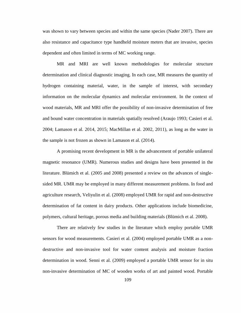
109

was shown to vary between species and within the same species (Nader 2007). There are

also resistance and capacitance type handheld moisture meters that are invasive, species

dependent and often limited in terms of MC working range.

MR and MRI are well known methodologies for molecular structure

determination and clinical diagnostic imaging. In each case, MR measures the quantity of

hydrogen containing material, water, in the sample of interest, with secondary

information on the molecular dynamics and molecular environment. In the context of

wood materials, MR and MRI offer the possibility of non-invasive determination of free

and bound water concentration in materials spatially resolved (Araujo 1993; Casieri et al.

2004; Lamason et al. 2014, 2015; MacMillan et al. 2002, 2011), as long as the water in

the sample is not frozen as shown in Lamason et al. (2014).

A promising recent development in MR is the advancement of portable unilateral

magnetic resonance (UMR). Numerous studies and designs have been presented in the

literature. Blümich et al. (2005 and 2008) presented a review on the advances of single-

sided MR. UMR may be employed in many different measurement problems. In food and

agriculture research, Veliyulin et al. (2008) employed UMR for rapid and non-destructive

determination of fat content in dairy products. Other applications include biomedicine,

polymers, cultural heritage, porous media and building materials (Blümich et al. 2008).

There are relatively few studies in the literature which employ portable UMR

sensors for wood measurements. Casieri et al. (2004) employed portable UMR as a non-

destructive and non-invasive tool for water content analysis and moisture fraction

determination in wood. Senni et al. (2009) employed a portable UMR sensor for in situ

non-invasive determination of MC of wooden works of art and painted wood. Portable

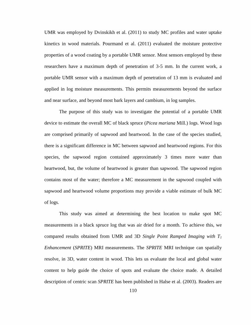
110

UMR was employed by Dvinskikh et al. (2011) to study MC profiles and water uptake


properties of a wood coating by a portable UMR sensor. Most sensors employed by these

researchers have a maximum depth of penetration of 3-5 mm. In the current work, a

portable UMR sensor with a maximum depth of penetration of 13 mm is evaluated and

applied in log moisture measurements. This permits measurements beyond the surface

and near surface, and beyond most bark layers and cambium, in log samples.

The purpose of this study was to investigate the potential of a portable UMR

device to estimate the overall MC of black spruce (Picea mariana Mill.) logs. Wood logs

are comprised primarily of sapwood and heartwood. In the case of the species studied,

there is a significant difference in MC between sapwood and heartwood regions. For this

species, the sapwood region contained approximately 3 times more water than

heartwood, but, the volume of heartwood is greater than sapwood. The sapwood region

contains most of the water; therefore a MC measurement in the sapwood coupled with

sapwood and heartwood volume proportions may provide a viable estimate of bulk MC

of logs.

This study was aimed at determining the best location to make spot MC

measurements in a black spruce log that was air dried for a month. To achieve this, we

compared results obtained from UMR and 3D Single Point Ramped Imaging with T1

Enhancement (SPRITE) MRI measurements. The SPRITE MRI technique can spatially

resolve, in 3D, water content in wood. This lets us evaluate the local and global water

content to help guide the choice of spots and evaluate the choice made. A detailed

description of centric scan SPRITE has been published in Halse et al. (2003). Readers are

111

referred to Lamason et al. 2014 for relevant discussions of SPRITE MRI and water

content in wood materials.


A freshly cut black spruce (Picea mariana Mill.) log of approximately 10.8 to

11.4 cm in diameter and 1.8 meters in length was employed for this study. The log was

harvested from the University of New Brunswick woodlot. The average gravimetric MC

of sapwood and heartwood were 130.4% and 41.5%, respectively. The fresh weight of

the log was 15.8 kg. Polyurethane reference markers on the log surface were used for

MRI image registration. They were fixed on the bark along a straight line for the full

length of the log. Adjacent markers were spaced approximately 3.8 cm apart. The log was

kept in an environmental chamber set at 20oC and 65% relative humidity for 7 months.

UMR and SPRITE MRI were undertaken after air drying for one month. The log ends

were wrapped with cellophane during UMR and MRI measurements to prevent moisture

loss at the ends during measurements.

The UMR measurements were performed with a three magnet array designed and

developed at the UNB MRI Centre. The device is lightweight, features open access, and

is portable (Marble et. al. 2007) (Figure 5-1). It produces a magnetic field along the

central vertical line above the surface of the unilateral magnet that is shown in Figure 5-2.

It shows that the unilateral magnet has a region of homogenous magnetic field, located

approximately 1.3 cm away from the top surface of the magnet. The radio frequency (RF)

coil in combination with the static field topology gives a sensitive spot for MR

112

measurement of approximately 1 cm3. This is significant because it allows measuring

signal within a finite volume inside the sample, not just from or near the surface.

The MR frequency in the sensitive spot was 4.46 MHz. The UMR measurements

were performed employing the Bruker Minispec console with a Carr Purcell Meiboom

Gill (CPMG) measurement that measures the transverse relaxation time T2 and signal

amplitude. The initial MR signal amplitude is proportional to moisture content. CPMG

measurement parameters were: 90° pulse length = 10µs, echo time = 160 µs, scans = 512,

and number of echoes = 1024. The acquisition time was approximately 10 min for each

UMR measurement.

113

Figure 5-1: Photograph of a unilateral magnet device employed in this study. The




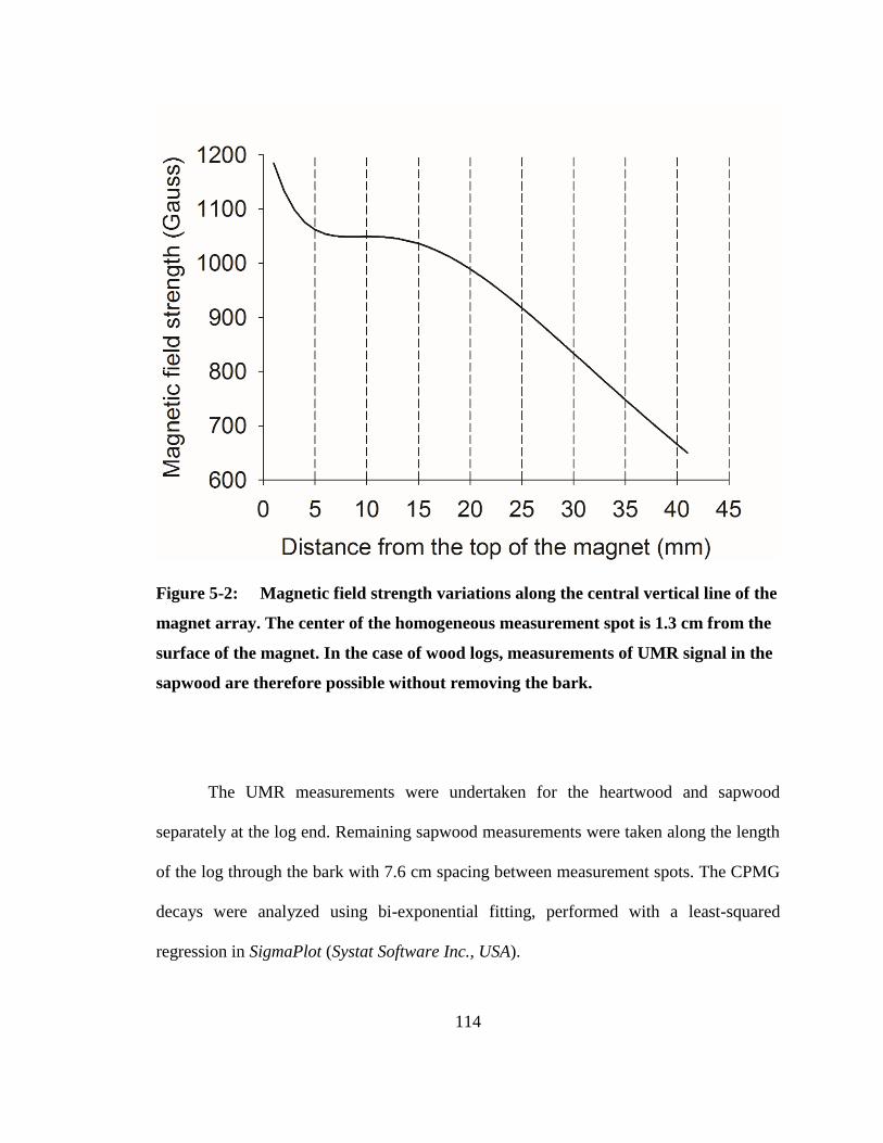
114

Figure 5-2: Magnetic field strength variations along the central vertical line of the

magnet array. The center of the homogeneous measurement spot is 1.3 cm from the

surface of the magnet. In the case of wood logs, measurements of UMR signal in the

sapwood are therefore possible without removing the bark.

The UMR measurements were undertaken for the heartwood and sapwood

separately at the log end. Remaining sapwood measurements were taken along the length

of the log through the bark with 7.6 cm spacing between measurement spots. The CPMG

decays were analyzed using bi-exponential fitting, performed with a least-squared

regression in SigmaPlot (Systat Software Inc., USA).

115

The decay constant is the T2 relaxation time. A bi-exponential fitting permits

determination of the relative hydrogen content in different environments (bound and

free), based on the lifetime of the MR signal. The short lifetime signal component is

related to the bound water, while the long lifetime signal component is related to the free

water (Lamason et al. 2015). The sum of the two signal populations are then converted

into MCs by using a reference sample of known MC. The reference sample has 30% MC

and is made of a mix of H2O, deuterium oxide (D2O), and copper sulfate.



water. There are two different types of lumen water. One is the bulk lumen water (2)



(conventionally called free water) is the weighted average rate of the surface water and

bulk water. Typically, there is more bulk water than surface water when the wood is

green, but the surface relaxation rate is much larger than the bulk relaxation rate. The

bulk and surface water in the lumen together are considered free water. Readers are

referred to Lamason et al. (2015) for relevant discussions on relaxation rates in wood.

The optimized CPMG measurements employed by the UMR allowed

quantification of both short and long lifetime signal components. The results of the UMR

measurements were compared to 3D SPRITE MRI images that were acquired using a

Nalorac (Nalorac Cryogenics Inc., Martinez, CA) 2.4 Tesla horizontal bore

superconducting magnet. The ambient temperature surrounding the sample was 12°C.

SPRITE 3D imaging parameters were: number of scans = 8, time between gradient steps

116

(TR) = 2 ms, maximum Tp, in an 8 point acquisition, = 264 µs, time between interleaves

= 500 ms, matrix size = 64 x 64 x 64, maximum gradient = 2.5 G/cm, field of view

(FOV) = 13 cm. The RF probe was a bird cage, 13 cm in diameter. The RF flip angle was

25°. The nominal image resolution was 0.2 cm per pixel and the total acquisition time

was 20 min for each image.


Typically, when wood is wet (green condition) the signal intensity measured with

the UMR in a CPMG measurement decayed bi-exponentially as shown in Figure 5-3. In

Figure 5-3 the short lifetime signal component, freshly cut black spruce sapwood, is

associated with the water in the cell walls while the long lifetime signal component is

associated with the lumen water (Riggin et al. 1979; Araujo et al. 1992; Lamason et al.

2015). The initial MR signal intensity is proportional to the overall quantity of water.

Total MC is equal to the sum of the signal from the two water environments. Signal

intensity decreased as the sample dried.

Optimization of the UMR CPMG measurement allows quantification of both

short and long lifetime signal components. Because the UMR measurements allowed

quantification of both short and long lifetime signal components, we can easily determine

the FSP for each species as the MC wherein the signal of the long lifetime component is

no longer observable while the short lifetime signal component remains at maximum

amplitude. Our earlier study, Lamason et al. (2015), with a non-optimized CPMG

measurement did not permit quantification of the short lifetime signal.

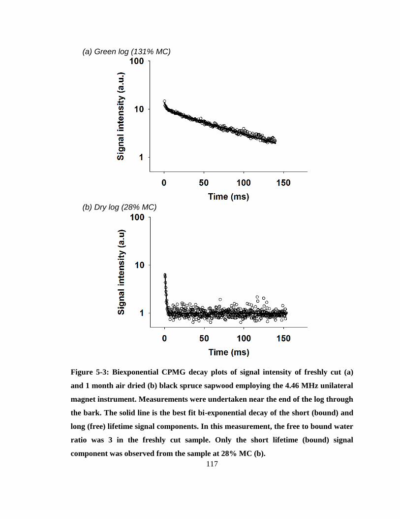
117

(a) Green log (131% MC)

(b) Dry log (28% MC)

Figure 5-3: Biexponential CPMG decay plots of signal intensity of freshly cut (a)

and 1 month air dried (b) black spruce sapwood employing the 4.46 MHz unilateral

magnet instrument. Measurements were undertaken near the end of the log through

the bark. The solid line is the best fit bi-exponential decay of the short (bound) and

long (free) lifetime signal components. In this measurement, the free to bound water

ratio was 3 in the freshly cut sample. Only the short lifetime (bound) signal

component was observed from the sample at 28% MC (b).

118

The data of Figure 5-3 were taken from a measurement spot near the end of the

log, through the bark. The measurement of Figure 5-3a corresponded to one day of drying

with a local MC of 131%. The measurement of Figure 5-3b corresponded to one month

of drying with a local MC of 28%. The MC of sapwood near the end of the log, through

the bark, was below FSP after one month of air drying.

At the initial sapwood MC, the ratio of the short and long lifetime signal

component was 1:3. This is due to the fact that at sapwood gravimetric MC of 130%, the

quantity of lumen water was a factor of 3.3 greater than the quantity of cell water,

assuming a FSP of approximately 30% MC.

The plot of Figure 5-3a shows that the spin-spin relaxation times of water in the

cell walls and in the lumen for black spruce sapwood ranged from 1 to 8 ms and 84 to 96

ms, respectively. These T2 values are in agreement with values published in the literature

for the signal lifetimes of water in wood (Riggin et al. 1979; Araujo et al. 1992; Zhang et

al. 2013; Lamason et al. 2015). The more mobile and accessible free water (lumen) has a

longer T2 than the bound water (cell wall).

The UMR signal intensity of the heartwood, taken from the end of the sample,

was low. The heartwood gravimetric MC is just slightly above FSP even with minimal

drying. MC measurements of heartwood are not indicative of the overall MC of the log.

The average initial MC of the log was 63.4%. This gravimetric MC was

determined from a 2.54 cm thick wood disk cut from each end of the log. The initial mass

of the log was 15.8 kg and the mass after one month in the environmental chamber was

14.8 kg. The calculated MC of the log after one month of drying was 52.6%.

119

Figure 5-4 is a plot of the measured total MC in sapwood as a function of position

along the length of the log, through the bark. A unilateral magnet utilizing CPMG

measurements was employed. As indicated in Figure 5-4, the near end surfaces of the log

were below 40% MC after one month of air drying. The MC of the spots 7.6 cm from the

ends were lower compared to the spots displaced away from the ends. Overall the signal

decreases from Day 1 to Day 30, however, for each drying time, the signal is spatially

uniform displaced from the ends. Surface or near surface measurements of water content

near the exposed end of a log are unreliable predictors of the bulk MC, since the end

surfaces dried more rapidly than the interior of the log. The interior looses moisture due

to capillary drying and radial drying, while losses from the end include diffusive losses.

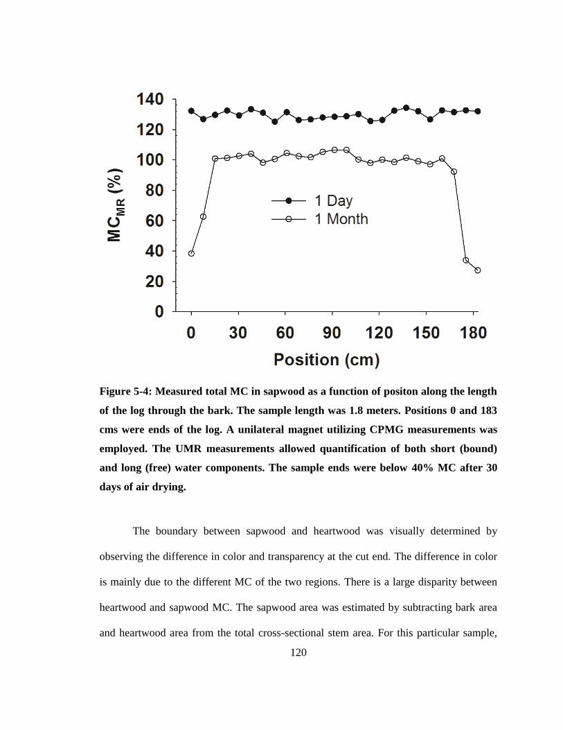
120

Figure 5-4: Measured total MC in sapwood as a function of positon along the length

of the log through the bark. The sample length was 1.8 meters. Positions 0 and 183

cms were ends of the log. A unilateral magnet utilizing CPMG measurements was

employed. The UMR measurements allowed quantification of both short (bound)

and long (free) water components. The sample ends were below 40% MC after 30

days of air drying.

The boundary between sapwood and heartwood was visually determined by

observing the difference in color and transparency at the cut end. The difference in color

is mainly due to the different MC of the two regions. There is a large disparity between

heartwood and sapwood MC. The sapwood area was estimated by subtracting bark area

and heartwood area from the total cross-sectional stem area. For this particular sample,

121

the ratio of sapwood to heartwood was 30:70 with respect to the overall volume of the

log. It was assumed that the log was cylindrical and that heartwood MC does not change

significantly unless the MC of the adjoining sapwood is below that of the heartwood. It is

therefore our proposal that a reliable estimation of MC of logs will include direct MC

measurement of sapwood and take into account the volume proportions of the heartwood

and sapwood regions. One difficulty with this approach is that not all species of wood

have a distinct boundary between sapwood and heartwood. For black spruce with a clear

distinction between heartwood and sapwood, a simple measurement approach as

described by equation 5-1 may be employed.

𝑀𝐶𝑙𝑜𝑔 = (𝑀𝐶𝑠𝑎𝑝𝑤𝑜𝑜𝑑 × 𝑉𝑜𝑙𝑠𝑎𝑝𝑤𝑜𝑜𝑑) + (𝑀𝐶ℎ𝑒𝑎𝑟𝑡𝑤𝑜𝑜𝑑 × 𝑉𝑜𝑙ℎ𝑒𝑎𝑟𝑡𝑤𝑜𝑜𝑑) (Equation 5-1)

where MClog is the overall MC of the log. MCsapwood and Volsapwood are moisture

content and volume of sapwood, respectively. MCheartwood and Volheartwood correspond to

moisture content and volume of heartwood. We measure the first term in equation 1 and

estimate the remaining terms assuming the heartwood is at fiber saturation.

The predicted MC of the log after a month of drying was 52.1 % based on the MC

estimation by UMR measurement in sapwood, coupled with sapwood to heartwood

volume proportions. This is remarkably close, given the assumptions, to the known

gravimetric value of 52.6%. It was assumed that in a log the heartwood MC does not

change significantly unless MC of the adjoining sapwood is below that of the heartwood.

MC of heartwood in the log was assumed to be 30%.

122

Figure 5-5 shows that the measured sapwood MC in a spot 15.2 cm from the end

was linearly related to the gravimetric MC of the whole log sample. The relationship is

clear especially during early times of air drying. This is due to the fact that most of the

water loss occurred in the sapwood and that the observed diffusive drying at the end

surfaces of the log does not significantly affect the overall MC during early stages of

drying. The exact position of the measured spot does not matter as long as it is displaced

from the ends. The UMR measurements in Figure 5-5 were undertaken at air drying times

which ranged from one day to seven months.

The relationship between the measured sapwood MC in a spot displaced from the

ends and the gravimetric MC was linear with a R2 of 0.98. Figure 5-5 gives a best fit line

of MCsapwood = 3.1 MCgravimetric - 65.7. In this linear equation, when sapwood is at FSP

(MCsapwood = 30%), the estimated MC of log (MCgravimetric) is 30.9%. This supports our

observation that as the log dries, most of the MC is lost in the sapwood when sapwood is

above FSP.

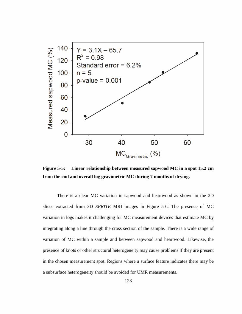
123

Figure 5-5: Linear relationship between measured sapwood MC in a spot 15.2 cm

from the end and overall log gravimetric MC during 7 months of drying.

There is a clear MC variation in sapwood and heartwood as shown in the 2D

slices extracted from 3D SPRITE MRI images in Figure 5-6. The presence of MC

variation in logs makes it challenging for MC measurement devices that estimate MC by

integrating along a line through the cross section of the sample. There is a wide range of

variation of MC within a sample and between sapwood and heartwood. Likewise, the

presence of knots or other structural heterogeneity may cause problems if they are present

in the chosen measurement spot. Regions where a surface feature indicates there may be

a subsurface heterogeneity should be avoided for UMR measurements.

124

The end images in Figure 5-6 also indicate the presence of a drying front in both

sapwood and heartwood. The drying front in sapwood extends several centimeters after

one month of drying. The presence of drying fronts at the ends of the log makes it very

difficult to estimate its MC if one uses a surface or near surface measurement at the end

of the log.

It is important to note that at the end of the log, the heartwood region that is close

to the sapwood has higher MC than heartwood regions away from the sapwood. This is

indicative of radial movement of moisture from the sapwood to the heartwood, possibly

along radial anatomical features such as wood rays. The 3D images show MC in

heartwood, away from end, does not change significantly while MC of sapwood is high.

The progression of the observed drying front in heartwood is slower than observed in

sapwood. This is because the initial MC of heartwood is lower than that of sapwood.

The 1D signal intensity profile in Figure 5-6 is an average of 5 profiles selected in

the sapwood region. The profile once again shows that the end dries more rapidly than

the sample interior. A few centimeters away from the end, the signal is remarkably

uniform along the length of the log.

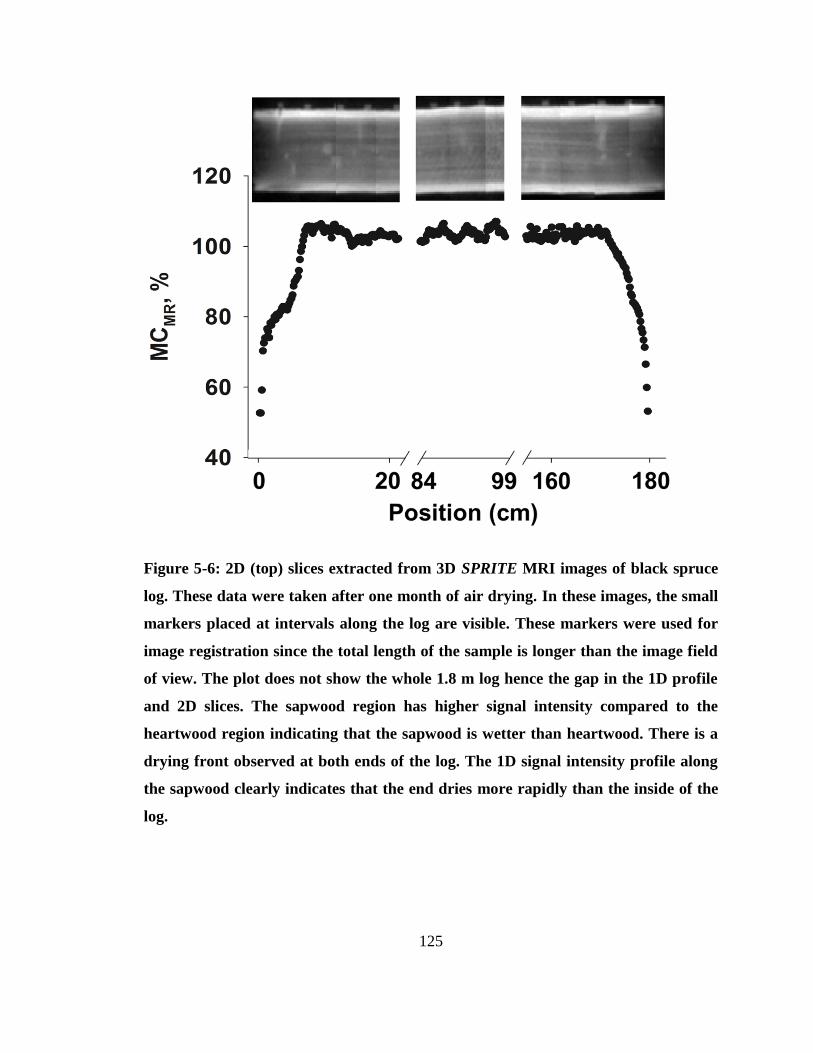
125

Figure 5-6: 2D (top) slices extracted from 3D SPRITE MRI images of black spruce

log. These data were taken after one month of air drying. In these images, the small

markers placed at intervals along the log are visible. These markers were used for

image registration since the total length of the sample is longer than the image field

of view. The plot does not show the whole 1.8 m log hence the gap in the 1D profile

and 2D slices. The sapwood region has higher signal intensity compared to the

heartwood region indicating that the sapwood is wetter than heartwood. There is a

drying front observed at both ends of the log. The 1D signal intensity profile along

the sapwood clearly indicates that the end dries more rapidly than the inside of the

log.

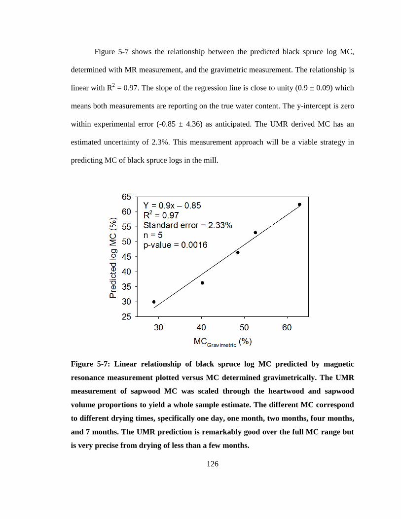
126

Figure 5-7 shows the relationship between the predicted black spruce log MC,

determined with MR measurement, and the gravimetric measurement. The relationship is

linear with R2 = 0.97. The slope of the regression line is close to unity (0.9 ± 0.09) which

means both measurements are reporting on the true water content. The y-intercept is zero

within experimental error (-0.85 ± 4.36) as anticipated. The UMR derived MC has an

estimated uncertainty of 2.3%. This measurement approach will be a viable strategy in

predicting MC of black spruce logs in the mill.

Figure 5-7: Linear relationship of black spruce log MC predicted by magnetic

resonance measurement plotted versus MC determined gravimetrically. The UMR

measurement of sapwood MC was scaled through the heartwood and sapwood

volume proportions to yield a whole sample estimate. The different MC correspond

to different drying times, specifically one day, one month, two months, four months,

and 7 months. The UMR prediction is remarkably good over the full MC range but

is very precise from drying of less than a few months.

127

5.4 Conclusions

It has been shown that MR and MRI are powerful tools for distinguishing and

mapping water in wood. Based on this study, the following conclusions can be made

about selecting a position or positions to make spot measurements to estimate bulk

moisture content in black spruce logs.

The UMR spot estimates of bulk MC in the sapwood of black spruce can be used

to estimate the overall MC of the black spruce log.

The ends and near ends through the bark of the log should be avoided in

estimating MC because of the presence of drying fronts. The drying front can extend up

to a few centimeters from the ends. Surface measurements are not adequate since there is

a wide variation of MC within a sample. A ‘through the bark’ measurement would be

ideal, especially if the device is able to directly measure sapwood. Likewise, one should

avoid regions with visual defects such as knots, reaction wood, excess resins, cracks, etc.

in choosing the spot to make MC measurements

In addition, we demonstrated the use of a portable UMR instrument as a powerful

tool in measuring MC in wood logs samples. This instrument has the advantage of

portability, permitting MC estimations in the field without oven drying. While we believe

the approach will be valid for black spruce, this may not be true for other species,

particularly hardwoods, where the difference in MC between the sapwood and heartwood

is species dependent. It is recommended that other important wood species be examined

in similar studies of log MC estimations.

128

The unilateral magnetic resonance method will allow measurement of water in

samples that are not debarked as it measures a volume located 1.3 cm below the surface,

which is a significant operational advantage.

Kinetic drying studies of wood can be further studied with the use of UMR and

MRI measurements as suggested by Figures 4 and 6. Likewise, existing drying models

can also be verified.

129

5.5 References

Araujo CD (1993) Proton magnetic resonance of wood and water in wood. Dissertation,

University of British Columbia

Blümich B, Casanova F, Perlo J, Anferova S, Anferov V, Kremer K, Goga N,

Kupferschlager K, Adams M (2005) Advances of unilateral mobile NMR in non-

destructive materials testing. Magn. Reson. Imaging 23(2): 197-201

Blümich B, Perlo J, Casanova F (2008) Mobile single-sided NMR. Progress in Nuclear

Magnetic Resonance Spectroscopy 52: 197-269

Bucur V (2003) Nondestructive characterization and imaging of wood. Springer Series in

Wood Science. Sringer-Verlag Berlin Heidelberg New York

Casieri C, Senni L, Romagnoli M, Santamaria U, DeLuca F (2004) Determination of

moisture fraction in wood by mobile NMR device. J. Magn. Reson 171(2): 364-

372

Cloutier A, Fortin Y (1991) Moisture content – water potential relationship of wood from

saturated to dry conditions. Wood Sci. and Tech 25(4):263-280

Droessler T, Bowyer JL, Burk T, Jamrock E, Antilla R (1986) Rate of weight loss in

piled pulpwood. Bull. AD-Sb-3036. Agri. Expt. Sta., Univ. of Minnesota, St.

Paul, MN. 18pp.

Dvinskikh SV, Furo I, Sandberg D, Soderstrom O (2011) Moisture content profiles and

uptake kinetics in wood cladding materials evaluated by a portable nuclear

magnetic resonance spectrometer. Wood Material Science and Engineering 6:

119-127

Fauchon T, Chantre G, Deleuze C (2000) How to control the variation of the wood

moisture content of logs from the stand to the wood yard? The contribution of

both direct techniques of assessment and modeling. In: Proc. Of the 2000 TAPPI

Pulping/Process and Product Quality Process. TAPPI Press, Atlant, GA, pp. 419-

431

Fortin Y (1979) Moisture content – matric potential relationship and water flow

properties of wood at high moisture contents. Dissertation, University of British

Columbia

Gingras JF, Sotomayor J (1992) Wood moisture variation in woodlands inventory: A case

study. Wood harvesting Tech. Note TN-192. Forest Engineering Res. Inst. of

Canada. Point Claire, QC, Canada. 6 pp.

130

Haddadi A, Hans G, Leblon B, Pirouz Z, Tsuchikawa S, Nader J, Groves K (2015)

Determination of optcal parameters and moisture content of wood with visible-

NIR spectroscopy. Submitted

Halse M, Goodyear DJ, MacMillan B, Szomolanyi P, Matheson D, Balcom BJ (2003)

Centric scan SPRITE magnetic resonance imaging. J Magn Reson 165(2):219-229

Hans G, Redman D, Leblon B, Nader J, La Rocque A (2015) Determination of log

moisture content using ground penetrating radar (GPR). Part 1. Partial least

squares (PLS) method. Holzforschung. doi:10.1515/hf-2014-0286






magnetic resonance devices. Wood Material Science and Engineering 10(1):86-

93. (also Chapter 4 of this Thesis)

MacMillan B, Schneider MH, Sharp AR,Balcom BJ (2002) Magnetic resonance imaging

of water concentration in low moisture content wood. Wood Fiber Science 2: 276-

286


resonance measurements of low moisture content wood. Canadian Journal of

Forest Research 41:2158-2162

Nader J (2007) Evaluation of two technologies to determine the moisture content of logs.

FPInnovations, Pointe-Claire, QC, Canada

Pourmand P, Wang L, Dvinskikh SV (2011). Assessment of moisture protective

properties of wood coatings by a portable NMR sensor. Journal of Coatings

Technology and Research 8(5): 649-654

Schultz EB, Matney TG, Watson WF (1997) Prediction of moisture contents for

sprinkled and un-sprinkled stacked roundwood over time. . In: Proc. TAPPI

Pulping Conf. TAPPI Press, Atlanta, GA. Pp 289-299

Senni L, Casieri C, Bovino A, Gaetani MC (2009) A portable NMR sensor for moisture

monitoring of wooden works of art, particularly of paintings on wood. Wood

Science and Technology 43: 167-180

Simpson WT, Wang X (2004) Estimating air-drying times of small diameter ponderosa

pine and Douglas-fir logs. Forest Products Journal 54(12):24-28

131

Tsuchikawa S, Torii M, Tsutsumi S (1996) Application of near-infrared

spectrophotometry to wood. 4. Calibration equations for moisture content. Journal

of the Japan Wood Research Society 42(8): 743–754

Veliyulin E, Mastikhin IV, Marble AE, Balcom BJ (2008) Rapid determination of the fat

content in packaged dairy products by unilateral NMR. Journal of the Science of

Food and Agriculture 88:2563-2567

Zhang J, Peralta PN (1999) Moisture content-water potential characteristic curves for red

oak and loblolly pine. Wood and Fiber Sci. 31(4):360-369

132

Chapter 6 – Magnetic resonance studies of wood log-drying processes

This chapter examines why the spot resolved black spruce sapwood measure of

MC gives good estimates of the whole black spruce log MC. The goal was to understand

drying behaviors of different regions in wood logs. This chapter provides spatially

resolved measurement (UMR and MRI) of MC as wood log dried. This chapter is largely

based on the paper “Magnetic resonance studies of wood log-drying processes” accepted

for publication in the Forest Products Journal. The format of references in this chapter

follows that of the original submission.

6.1 Introduction

Wood is a naturally occurring composite material which is hygroscopic and

anisotropic with properties that are deeply influenced by the presence of water.

Measurements of moisture content (MC) of wood are therefore of considerable

importance. Like most natural porous materials, wood undergoes drying from its natural

state to end use state. Drying processes involve the removal of moisture from the material

through a variety of mechanisms, such as capillary flow and diffusion. These processes

are of critical importance for wood which must be dried from its green MC prior to use as

a fuel or as a construction material (FPL 2010).

The pores in wood can be filled with air or vapor, but may also be partially or

fully filled with liquid water. Water in wood exists in two different environments: (1) in

the cell wall as cell wall water and (2) as lumen water in the cell lumens and other void

spaces (Siau 1971, Panshin and de Zeeuw 1980, FPL 2010). The maximum water content

133

in the cell wall is termed the fiber saturation point (FSP) and occurs around 30% MC for

most species (Skaar 1988). The FSP is a critical parameter since most properties of wood

are altered by changes in MC below the FSP.

Capillary forces determine the movement of lumen water. As wood dries,

evaporation of water from the surface sets up capillary forces that exert a pull on the

lumen water in zones beneath the surface (Panshin and de Zeeuw 1980, Skaar 1988).

When there is no longer any lumen water in the wood capillary forces are no longer of

importance. As cell wall water is removed by diffusion, the wood shrinks. A number of

physical and mechanical properties of wood are independent of MC at MCs higher than

the FSP, but these properties are found to change at lower MCs as the cell wall water is

removed (Siau 1971 and FPL 2010).

Drying of materials is often studied by handheld moisture meters that measure the

water content by indirect methods, relying on the fact that the electrical properties of the

material are dependent on the water content. However, these instruments are not able to

monitor the whole drying process because they are limited in effective MC range; they

are point measurements; and they are in some cases intrusive. Recent developments in

magnetic resonance (MR) permit monitoring the local MC (Lamason et al 2014) with a

more direct and non-intrusive approach.

Several MR and magnetic resonance imaging (MRI) studies on wood have been

reported in the literature. Conventional MR and MRI techniques were employed to study

wood anatomy and structure (Wang and Chang 1986, Hall et al 1986, Flibotte et al.

1990), wood decay (Flibotte et al. 1990), and wood preservation (Meder et al. 1999).

134

With respect to MC estimation, MR/MRI techniques have been used to estimate MC in

wood pellets (Nyström and Dahlquist 2004) and in wood drying (Araujo et al. 1992, Hall

et al. 1986, Menon et al. 1989, Quick et al. 1990, Hartley et al. 1993, Hameury et al.

2006, Almeida et al. 2007, Stenstrom et al. 2009, Passarini et al. 2014 and 2015). Most of

these studies consider relatively wet wood because conventional MRI techniques are not

quantitative at low MCs.

Portable unilateral magnetic resonance (UMR) is a promising new development in

MR. Numerous studies and magnet designs have been presented in the literature.

Blümich et al. (2005 and 2008) has recently reviewed single-sided MR. UMR may be

employed in many different measurement problems. In food and agriculture research,

Veliyulin et al. (2008) employed UMR for rapid and non-destructive determination of fat

content in dairy products. Other applications include biomedicine, polymers, cultural

heritage, porous media and building materials (Blümich et al. 2008).

Lamason et al. (2015) employed UMR to study water states and water content of

black spruce (Picea mariana Mill.) and aspen (Populus tremuloides Michx.). They found

a bi-exponential decay of the time-domain MR measurements which was attributed to the

cell wall water (short lifetime signal) and cell lumen water (long lifetime signal).

In the current work, a portable UMR sensor and MRI measurement techniques

were employed to study drying behaviour during air drying of black spruce (Picea

mariana Mill.) log. Results from UMR were compared to 3D centric scan Single Point

Ramped Imaging with T1 Enhancement (SPRITE) MRI measurements. The SPRITE MRI

technique can spatially resolve, in 3D, total water content in wood. A detailed description

of centric scan SPRITE has been published in Halse et al. (2003). Readers are referred to

135

Lamason et al. (2014) for relevant discussions of SPRITE MRI and water content

measurements in wood materials.

There are several log drying models which have been presented in the literature.

Droessler et al. (1986) investigated the influence of weather conditions on drying rates.

They found that the rate of weight loss in freshly cut, piled wood log was largely

constant, but was influenced by environmental conditions, such as average daily high

temperature, average high humidity, and total rainfall in the days immediately preceding

measurement. Fauchon et al. (2000), developed a model to estimate the drying rate of

logs during storage. Their model takes into account the initial MC and relative humidity

of ambient air. Simpson and Wang (2004) developed a model to predict air-drying times

of small diameter ponderosa pine and Douglas-fir logs. Schultz et al. (1997) developed a

more advanced model and reported that species, days in storage, and log diameter had the

greatest effects on drying behavior, while the effect of drying through log ends on overall

log moisture loss was relatively minor. Schultz et al. (1997) argued that the radial drying

through the bark dominates because 1) radial distances from the log center to the bark

provided a much shorter path for water evaporation than longitudinal travel; 2) the

surface area for radial moisture paths was many times greater than the surface area of log

ends. Radial gradients in MC were observed by Schultz et al. (1997) through coarse

sectioning and drying. Defo and Brunette (2006) developed a log drying model based on

the concept of water potential. They presented simulations of the effect of bark loss on

drying.

136

Simple mass measurements were employed by the authors of the above models.

They assume the wood log is a homogenous cylinder with a single type of water. These

assumptions automatically preclude a realistic model. Wood consists of sapwood and

heartwood that will have different drying behaviors and water in wood exists in two

different environments (cell wall and cell lumen) with different physical behaviors. In

addition, the majority of traditional measurements have coarse spatial resolution and

cannot observe moisture gradients. While the above assumptions may be reasonable to a

first approximation they preclude a more rigorous examination of mechanisms and

thereby the assembly of high quality drying models. Measurements which permit

differentiation of sapwood and heartwood, which distinguish cell wall and cell lumen

water, while measuring local MC and MC gradients will be invaluable to evaluate drying

mechanisms and to help assemble future drying models.

This study was aimed at understanding the behavior of water in black spruce

wood logs during drying. The UMR and MRI measurements were employed to spatially

resolve water content in a black spruce (Picea mariana Mill.) log. These measurements

allowed quantification of water content in sapwood and heartwood regions and, in the

case of UMR measurements, differentiated cell wall and cell lumen water. This

experimental data will help improve existing wood drying models for better and more

accurate predictions of water content. Although this study was designed to understand

drying mechanisms in wood logs, the UMR and MRI measurements can easily be

translated to lumber and other wood products.

137


A freshly cut black spruce butt log approximately 10.8 to 11.4 cm in diameter and

1.8 meters in length was employed for this study. The log had approximately 80 growth

rings at cross section. The fresh weight of the log was 15.8 kg. Two 2.5-cm thick disks,

one from each end, were cut for gravimetric MC measurements. Polyurethane reference

markers on the log surface were employed for MRI image registration. Markers were

fixed on the bark in a straight line for the full length of the log. Adjacent markers were

spaced 3.8 cm apart. The log was maintained in an environmental chamber set at 20oC

and 65% relative humidity. UMR and SPRITE MRI measurements were undertaken

during air drying over a four month period. All measurements were undertaken in the

laboratory with the log maintained in an environmental chamber for the entire study. The

log ends were wrapped with cellophane during UMR and MRI measurements to prevent

moisture loss during measurement.

The UMR measurements were performed with a three magnet array UMR device

developed at the University of New Brunswick MRI Centre. The device is lightweight,

features open access, and is portable (Marble et. al. 2007). It produces a uniform

magnetic field of 0.1 Tesla, located approximately 1.3 cm measured from the top surface

of the magnet. The radio frequency coil in combination with the static field topology

gives a sensitive spot for MR measurement of approximately 1 cm3. This permits signal

to be measured within a finite volume inside the sample at a fixed depth within the log.

Figure 6-1 shows a schematic diagram of a cross section of wood log and UMR showing

the sensitive spot displaced from the surface of the magnet with respect to the different

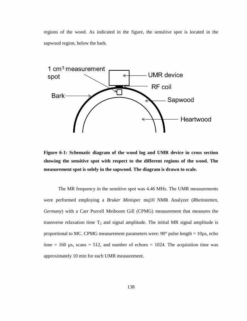
138

regions of the wood. As indicated in the figure, the sensitive spot is located in the

sapwood region, below the bark.

Figure 6-1: Schematic diagram of the wood log and UMR device in cross section

showing the sensitive spot with respect to the different regions of the wood. The

measurement spot is solely in the sapwood. The diagram is drawn to scale.

The MR frequency in the sensitive spot was 4.46 MHz. The UMR measurements

were performed employing a Bruker Minispec mq10 NMR Analyzer (Rheinstetten,

Germany) with a Carr Purcell Meiboom Gill (CPMG) measurement that measures the

transverse relaxation time T2 and signal amplitude. The initial MR signal amplitude is

proportional to MC. CPMG measurement parameters were: 90° pulse length = 10µs, echo

time = 160 µs, scans = 512, and number of echoes = 1024. The acquisition time was

approximately 10 min for each UMR measurement.

139

The UMR measurements were undertaken for sapwood along the length of the

log, through the bark, with 7.6 cm spacing between measurement spots. The CPMG

decays were analyzed using a bi-exponential fitting, performed with a least squares

regression in SigmaPlot (Systat Software Inc., USA).

The CPMG decay constant is the T2 relaxation time. A bi-exponential fitting

permitted determination of the relative water content in different environments (cell wall

and cell lumen), based on the lifetime of the MR signal. The short lifetime signal

component is related to the cell wall water, while the long lifetime signal component is

related to the lumen water (Lamason et al. 2015). The sum of the two signal populations

were then converted into MCs by using a reference sample of known MC. The reference

sample had 30% MC and was fabricated from a mix of H2O, deuterium oxide (D2O), and

copper sulfate.

The CPMG measurements employed by the UMR allowed quantification of both

short and long lifetime signal components. The UMR measurements were compared to

3D SPRITE MRI images acquired using a Nalorac (Nalorac Cryogenics Inc., Martinez,

CA) 2.4 Tesla horizontal bore superconducting magnet. The ambient temperature was

12°C. SPRITE 3D imaging parameters were: number of scans = 8, time between gradient

steps (TR) = 2 ms, maximum Tp, in an 8 point acquisition, = 264 µs, time between

interleaves = 500 ms, matrix size = 64 x 64 x 64, maximum gradient = 2.5 G/cm, field of

view (FOV) = 13 cm. The RF probe was a bird cage, 13 cm in diameter. The RF flip

angle was 25°. The nominal image resolution was 0.2 cm per pixel and the total

acquisition time was 20 min for each image.

140

The SPRITE MRI measurement was three dimensional encompassing the entire

wood cross sectional volume while the UMR measurement was limited to a relatively

large sensitive volume in the near surface sapwood, below the bark. The UMR

measurement spot is translated longitudinally from one end of the log to the other.


The gravimetric MC of the fresh log was 63% based on the average of two 2.5 cm

thick wood disks, one from each end, cut from the log. The bark thickness was

approximately 2 mm. The sapwood thickness was approximately 1.5 cm.

The UMR CPMG measurement of a freshly cut log revealed an MR signal that

decayed bi-exponentially as shown in Figure 6-2. The short lifetime signal component

from a freshly cut black spruce sapwood is associated with the water in the cell walls

while the long lifetime signal component is associated with the lumen water (Riggin et al.

1979; Menon et al. 1987 and 1989; Araujo et al. 1992; Lamason et al. 2015). The initial

MR signal intensity is proportional to the overall quantity of water. The total MC is equal

to the sum of the signal from the two water environments. Signal intensity decreased as

the sample dried. No signal was detected from the long lifetime signal component at a

MC lower than 15% (Figure 6-2b). At initial MC the ratio of cell wall to lumen water in

the sapwood, along the length of the log, ranged from 1:3.0 to 1:3.4. This ratio was

computed based on the y-intercepts of the short and long lifetime signal components of

the CPMG decay. This is consistent with the conceptual definition of FSP. At a MC of

132%, the lumen water quantity is greater by a factor of 3.4, compared to the cell wall

141

water, assuming a FSP of around 30% MC. At initial conditions, the observed T2 values

of short (cell wall) and long (lumen) lifetime signal components ranged from 1 ms to 8

ms and 84 ms to 96 ms, respectively.

The observed relaxation rate (1

𝑇2) from the water in the lumen (free water) is the

weighted average rate of both the surface and bulk water (Menon et al. 1987; Wong

1999). Typically, there is more bulk water in the cell volume than surface water when the

wood is green, but the surface relaxation rate is much greater than the bulk relaxation

rate. As lumen water is removed, the average T2 of the long lifetime signal component

decreases because the surface water contribution to T2 increases in significance.

A bi-exponential fitting of the CPMG decay gave a satisfactory fit to the

experimental decay. This was supported by a high R2, low standard error of estimate, and

analysis of variance results. Previous work on spin-spin relaxation rates in wood

suggested that MR measurements could differentiate lumen water in earlywood and

latewood due to different cell cavity sizes. However, three discrete exponentials were not

observed in the current work. Menon et al. (1987 and 1989) assigned earlywood and

latewood lumen water (different cell cavity sizes) to the longer two of three observed

time constants in their work. In the current work, we were unable to resolve separately

earlywood and latewood contributions. We assume that the long lifetime T2 observed and

reported is an average of the cell lumen water in earlywood and latewood.

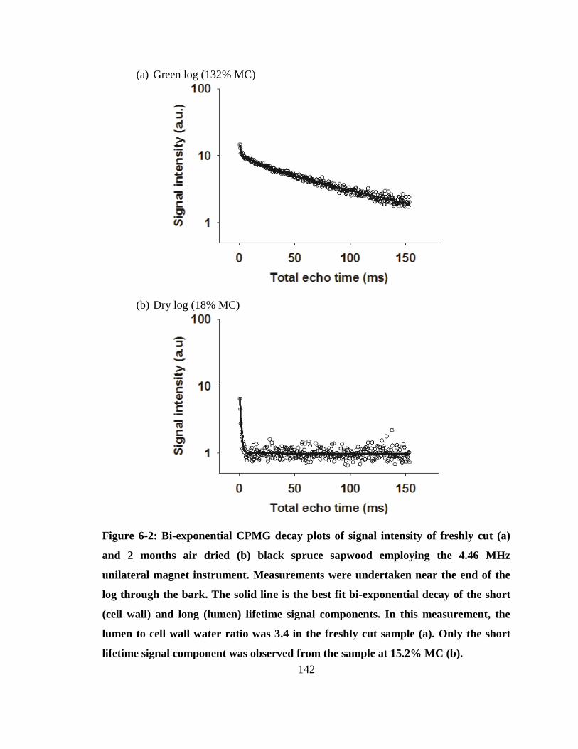
142

(a) Green log (132% MC)

(b) Dry log (18% MC)

Figure 6-2: Bi-exponential CPMG decay plots of signal intensity of freshly cut (a)

and 2 months air dried (b) black spruce sapwood employing the 4.46 MHz

unilateral magnet instrument. Measurements were undertaken near the end of the

log through the bark. The solid line is the best fit bi-exponential decay of the short

(cell wall) and long (lumen) lifetime signal components. In this measurement, the

lumen to cell wall water ratio was 3.4 in the freshly cut sample (a). Only the short

lifetime signal component was observed from the sample at 15.2% MC (b).

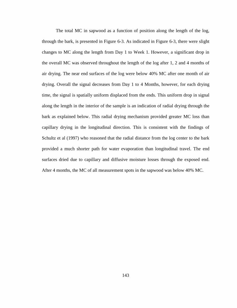
143

The total MC in sapwood as a function of position along the length of the log,

through the bark, is presented in Figure 6-3. As indicated in Figure 6-3, there were slight

changes to MC along the length from Day 1 to Week 1. However, a significant drop in

the overall MC was observed throughout the length of the log after 1, 2 and 4 months of

air drying. The near end surfaces of the log were below 40% MC after one month of air

drying. Overall the signal decreases from Day 1 to 4 Months, however, for each drying

time, the signal is spatially uniform displaced from the ends. This uniform drop in signal

along the length in the interior of the sample is an indication of radial drying through the

bark as explained below. This radial drying mechanism provided greater MC loss than

capillary drying in the longitudinal direction. This is consistent with the findings of

Schultz et al (1997) who reasoned that the radial distance from the log center to the bark

provided a much shorter path for water evaporation than longitudinal travel. The end

surfaces dried due to capillary and diffusive moisture losses through the exposed end.

After 4 months, the MC of all measurement spots in the sapwood was below 40% MC.

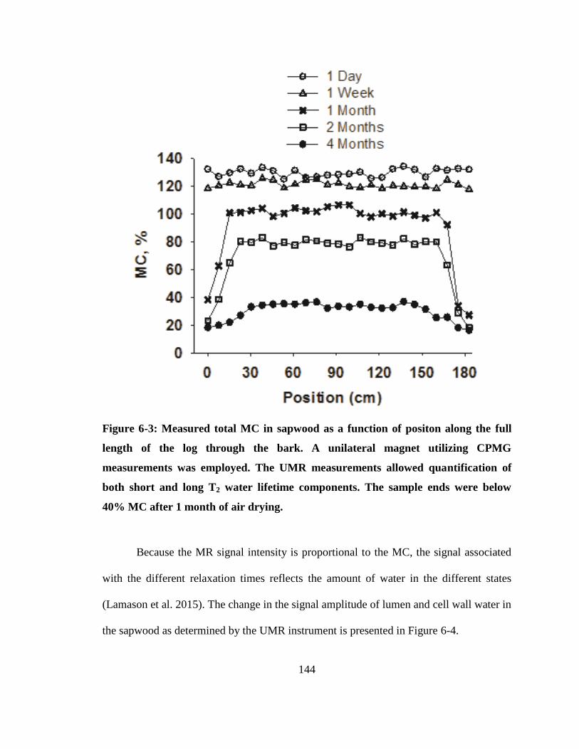
144

Figure 6-3: Measured total MC in sapwood as a function of positon along the full

length of the log through the bark. A unilateral magnet utilizing CPMG

measurements was employed. The UMR measurements allowed quantification of

both short and long T2 water lifetime components. The sample ends were below

40% MC after 1 month of air drying.

Because the MR signal intensity is proportional to the MC, the signal associated

with the different relaxation times reflects the amount of water in the different states

(Lamason et al. 2015). The change in the signal amplitude of lumen and cell wall water in

the sapwood as determined by the UMR instrument is presented in Figure 6-4.

145

No signal was detected from the sapwood lumen water at both ends of the log

after 2 months of air drying (Figure 6-4d). Initially, the MC of sapwood along the length

of the log ranged from 125 to 135%. The cell wall water signal intensity did not change

significantly above 30% MC. This result is in agreement with Zhang et al. (2013) and

Lamason et al. (2015) who reported that cell wall water does not change significantly

above 40% MC. No signal from lumen water was detected at or below 20% MC. The cell

wall MC did not change significantly in the early stages of drying. After one month of

drying, the cell wall MC was below FSP at both ends of the log. After 4 months, minimal

lumen water was observed in all the measurement spots along the full length of the log.

At initial conditions, the T2 value of cell wall water is constant (not shown in

Figure 6-4). Lumen water T2 ranged from 84 ms to 96 ms at initial conditions; however,

as lumen water is removed during drying the corresponding T2 decreases. The T2

decreases because the surface to volume ratio changes as water only fills part of the cell

volume. The T2 of a particular cell cavity size will decrease as water is removed. A

partially filled cavity will have a shorter T2 than a fully saturated cavity.

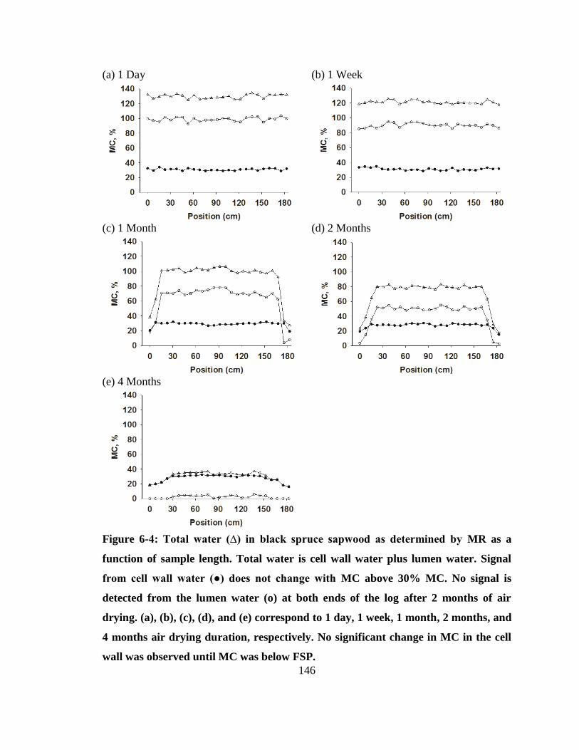
146

(a) 1 Day (b) 1 Week

(c) 1 Month (d) 2 Months

(e) 4 Months

Figure 6-4: Total water (∆) in black spruce sapwood as determined by MR as a

function of sample length. Total water is cell wall water plus lumen water. Signal

from cell wall water (●) does not change with MC above 30% MC. No signal is

detected from the lumen water (o) at both ends of the log after 2 months of air

drying. (a), (b), (c), (d), and (e) correspond to 1 day, 1 week, 1 month, 2 months, and

4 months air drying duration, respectively. No significant change in MC in the cell

wall was observed until MC was below FSP.

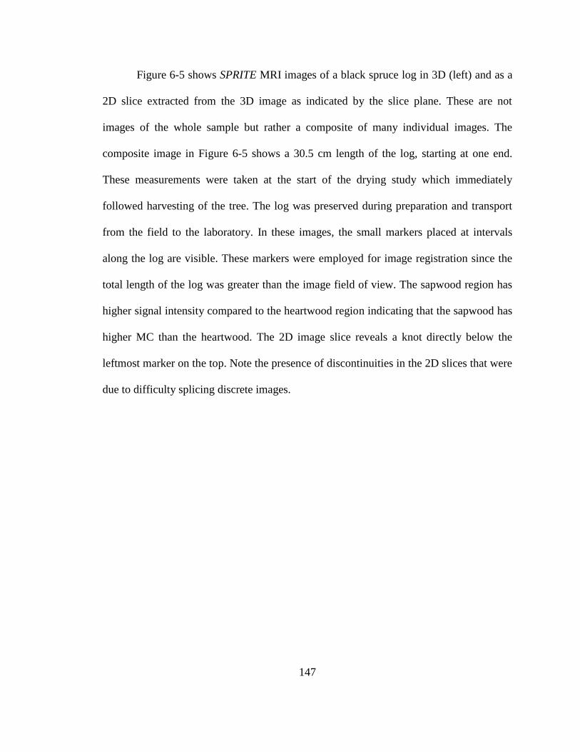
147

Figure 6-5 shows SPRITE MRI images of a black spruce log in 3D (left) and as a

2D slice extracted from the 3D image as indicated by the slice plane. These are not

images of the whole sample but rather a composite of many individual images. The

composite image in Figure 6-5 shows a 30.5 cm length of the log, starting at one end.

These measurements were taken at the start of the drying study which immediately

followed harvesting of the tree. The log was preserved during preparation and transport

from the field to the laboratory. In these images, the small markers placed at intervals

along the log are visible. These markers were employed for image registration since the

total length of the log was greater than the image field of view. The sapwood region has

higher signal intensity compared to the heartwood region indicating that the sapwood has

higher MC than the heartwood. The 2D image slice reveals a knot directly below the

leftmost marker on the top. Note the presence of discontinuities in the 2D slices that were

due to difficulty splicing discrete images.

148

Figure 6-5: SPRITE MRI composite images of a black spruce log in 3D (left) and 2D

slice extracted from the 3D image on the left as indicated by the slice plane. These

are not images of the entire log sample. These joined images represent 30.5 cm of

the log length, starting at one end. Measurements were taken at the start of the

drying study. In these images, the small markers placed at intervals along the log

are visible. These markers were used for image registration since the total length of

the sample is longer than the image field of view. The sapwood region has higher

signal intensity compared to the heartwood region indicating that the sapwood has

high MC.

MC in sapwood (Figure 6-6a) and heartwood (Figure 6-6b) as a function of

position along the length of the log is given in Figure 6-6. Positions 0 and 91 cm

correspond to the end and midpoint along the length, respectively. These 1D profiles

were averages of three profiles along the sapwood and were extracted from the 3D

SPRITE MRI composite images. A decrease in MC was observed with increased drying

duration. Diffusive drying was observed at the end of the sample and is immediately

apparent at Day 1. Both Figure 6-3 and Figure 6-6a reveal uniform water content and

uniform water loss, except at the ends. For sapwood (Figure 6-6a), the diffusive drying

front has penetrated approximately 9 cm from the end after one month of air drying. For

149

heartwood (Figure 6-6b) the diffusive drying front penetrated from the end within one

week of air drying. The MC of heartwood in the interior is constant until after 2 months

of air drying. Although diffusive end drying was immediately apparent at early drying

times, the more significant loss of MC was observed in the radial direction of the log (as

discussed below).

Figure 6-7 shows SPRITE MRI images of the black spruce log in the transverse

direction (left) and radial profiles (right) extracted from the image at the central vertical

line of the image, for three positions along the length of the log. These data were taken

after one month of air drying. The sapwood region has higher signal intensity compared

to the heartwood region indicating that the sapwood has higher MC than heartwood.

There is a drying front observed near the end of the log. The MC in the sapwood and

heartwood regions at the end of the log is less than the MC in regions displaced from the

end. Heterogeneity in MC in the heartwood region is apparent from variation in image

intensity in the 2D slices, as well as in the radial profiles. The bottom MRI image shows

the presence of knots in the transverse plane. The end and heartwood portion of the knots

appeared to have drier regions compared to the neighboring sapwood.

150

(a) Sapwood

(b) Heartwood

Figure 6-6: MC in sapwood (a) and heartwood (b) as a function of position along the

length of the log. Positions 0 and 91 cms correspond to the end and midpoint along

the length, respectively. These 1D profiles were extracted from the 3D SPRITE MRI

images. A decrease in MC was observed with increased drying duration. Diffusive

drying was observed at the end of the sample.

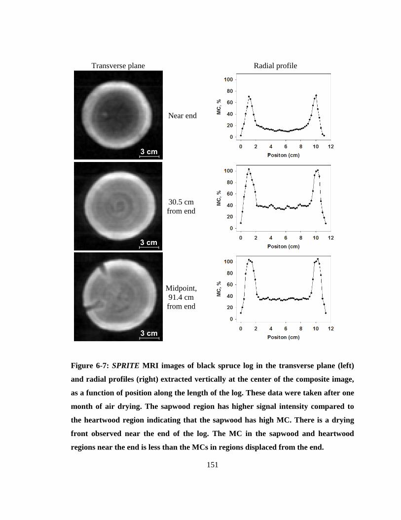
151

Transverse plane Radial profile

Near end

30.5 cm

from end

Midpoint,

91.4 cm

from end

Figure 6-7: SPRITE MRI images of black spruce log in the transverse plane (left)

and radial profiles (right) extracted vertically at the center of the composite image,

as a function of position along the length of the log. These data were taken after one

month of air drying. The sapwood region has higher signal intensity compared to

the heartwood region indicating that the sapwood has high MC. There is a drying

front observed near the end of the log. The MC in the sapwood and heartwood

regions near the end is less than the MCs in regions displaced from the end.

152

Radial drying through the bark was observed during the course of the drying

study. Figure 6-8 gives the MC profiles in the vertical direction corresponding to the

central transverse plane of the log (refer to Figure 6-7). The location of the UMR

sensitive spot measurement is noted in the figure. It is located in the sapwood below the

bark. The UMR measurement averages the MC in the sensitive spot. This figure shows

the MC varies radially within the region of sample measured by UMR. The UMR

measurements provide an average signal from a gradient of MC as revealed in the MRI

SPRITE measurement. MC decreases with air drying duration. A moisture gradient

through the sapwood in the radial direction was observed due to diffusive drying through

the bark. Anatomical features such as rays are responsible for the movement of water

through the bark (Panshin AJ and de Zeeuw C 1980). The MC in the heartwood region,

midpoint along the length of the log, is constant up to two months of drying. Away from

the sample ends, the MC of the heartwood only decreases once the MC of the adjoining

sapwood is below that of the heartwood.

In the field, a UMR measurement to estimate the log MC may be problematic.

Logs in the field or mill yard are usually stack piled and access to regions of the log

surface displaced from the end may be impossible. End measurement of MC is not

representative of the overall log MC.

153

Figure 6-8: MC in the vertical direction, corresponding to the central transverse

plane of the log at the midpoint along its length. A moisture gradient through the

sapwood in the radial direction is observed due to diffusive drying through the

bark. MC decreases with air drying duration. In heartwood, no significant change

in MC was observed at early drying times, however, a drop in MC was observed

after 4 months of air drying. The position of the UMR sensitive spot is illustrated.

Data for heartwood MC, not the sapwood, was smoothed with a 3-point moving

averaged.

154

6.4 Conclusions

The application of MR measurement techniques in the study of a wood log drying

allowed better understanding of its drying mechanisms. Both the UMR and SPRITE MRI

results are in agreement pertaining to the observed drying behavior and MC estimation.

There is evidence of diffusive end drying and radial drying through the bark. The effect

of radial drying through the bark is more significant compared to the diffusive end drying

even though the diffusive end drying was immediately apparent from Day 1.

The sapwood region has higher signal intensity compared to the heartwood region

indicating that the sapwood has higher MC than heartwood. Results indicated that

diffusive drying occurred at the ends of the log for both sapwood and heartwood.

Substantial radial drying through the bark was observed in the interior of the log. The

water content in the cell wall does not change significantly until lumen water is depleted.

Though this work considers a wood log as the sample, we infer that MR and MRI

measurements of MC employed here can be translated to other wood materials such as

lumber, timber, engineered wood products and composites, where non-destructive and

direct water content measurements is of vital significance.

The UMR and MRI measurements employed allowed spatially resolved

measurements of MC which is beneficial in determining and understanding the MC

gradients present in the sample. Traditional wood drying models employ mass

measurements, destructive techniques and bulk MC measurements which automatically

make determination of MC gradients problematic.

In addition, we have demonstrated that the UMR and MRI measurements are

powerful tools that can be employed to verify existing wood drying models. Based on

155

this study, a good drying model should include drying behaviors of cell wall and lumen

water as well as drying kinetics present in sapwood and heartwood regions.

156

6.5 References

Almeida, G., S. Gagne, and R. E. Hernández.2007. A NMR study of water distribution in

hardwoods at several equilibrium moisture contents. Wood Sci Technol 41(4):293-307.

Araujo, C. D., A. L. MacKay, J. R. T. Hailey, K. P. Whittall, and H. Le. 1992. Proton

magnetic resonance techniques for characterization of water in wood: application to

white spruce. Wood Sci. Technol. 26(2):101-113.

Blümich, B., F. Casanova, J. Perlo, S. Anferova, V. Anferov, K. Kremer, N. Goga, K.

Kupferschlager, and M. Adams.2005. Advances of unilateral mobile NMR in non-

destructive materials testing. Magn. Reson. Imaging 23(2):197-201.

Blümich, B., J. Perlo, and F. Casanova. 2008. Mobile single-sided NMR. Progress in

Nuclear Magnetic Resonance Spectroscopy 52:197-269.

Defo, M., and G. Brunette. 2006. A log drying model and its application to the simulation

of the impact of bark loss. Forest Prod. J. 56(5):71-77.

Droessler, T., J. L. Bowyer, T. Burk, E. Jamrock, and R. Antilla. 1986. Rate of weight

loss in piled pulpwood. Bull. AD-Sb-3036. Agri. Expt. Sta., Univ. of Minnesota, St. Paul,

MN. 18pp.

Fauchon, T., G. Chantre, and C. Deleuze. 2000. How to control the variation of the wood

moisture content of logs from the stand to the wood yard? The contribution of both direct

techniques of assessment and modeling. In: Proc. Of the 2000 TAPPI Pulping/Process

and Product Quality Process. TAPPI Press, Atlant, GA, pp. 419-431.

FPL (2010) Wood handbook – Wood as an engineering material. Gen Tech Rep FPL-


Flibotte, S., R. S. Menon, A. L. MacKay, and J. R. T. Hailey. 1990. Proton magnetic

resonance of western red cedar. Wood Fiber Sci 22(4):362-376.

Hall, L. D., V. Rajanayagam, W. A. Stewart, and P. R. Steiner.1986. Magnetic resonance

imaging of wood. Can J Forest Res 16(2):423-426.

Halse, M., D. J. Goodyear, B. MacMillan, P. Szomolanyi, D. Matheson, and B. J.

Balcom. 2003. Centric scan SPRITE magnetic resonance imaging. J Magn Reson

165(2):219-229.

Hameury, S., and M. Sterley. 2006. Magnetic resonance imaging of moisture distribution

in Pinus sylvestris L. exposed to daily indoor relative humidity fluctuations. Wood Mater

Sci Eng, 1:116-126.

157

Hartley, I.D., F. A. Kamke, and H. Peemoeller. 1993. Absolute moisture content



Lamason, C., B. MacMillan, B. J. Balcom, B. Leblon, and Z. Pirouz.2014. Examination

of water phase transitions in black spruce by magnetic resonance and magnetic resonance


Lamason, C., B. MacMillan, B. J. Balcom, B. Leblon, and Z. Pirouz. 2015. Water content

measurement in black spruce and aspen sapwood with bencthtop and portable magnetic

resonance devices. Wood Material Science and Engineering 10(1):86-93. (also Chapter 4

of this Thesis)

Marble, A. E., I. V. Mastikhin, B. G. Colpitts, and B. J. Balcom. 2007. A compact

permanent magnet array with a remote homogenous field. J Magn Reson 186 (1):100-

104.

Meder, R., R. A. Franich, and P. T. Callaghan. 1999. 11

B magnetic resonance imaging

and MAS spectroscopy of trimethylborate-treated radiate pine wood. Solid State Nucl

Magn Reson 15 (1):69-72.

Menon, R. S., A. L. MacKay, J. R. T. Hailey, M. Bloom, A. E. Burgess, and J. S.

Swanson. 1987. An NMR determination of the physiological water distribution in wood

during drying. J Appl Polym Sci 33:1141-1155.

Menon, R. S., A. L. Mackay, S. Flibotte, and J. R. T. Hailey. 1989. Quantitative

separation of NMR images of water in wood on the basis of T2. J. Magn. Reson 82:205-

210.

Nyström, J., and E. Dahlquist. 2004. Methods for Determination of moisture content in

wood chips for power plants - a Review. Fuel (83):773–779.

Panshin, A. J., and C. de Zeeuw. 1980. Textbook of Wood Technology. 4th

Ed. McGraw-

Hill Publishing Company. pp. 722.

Passarini, L., C. Malveau, and R. E. Hernández. 2014. Water state study of wood

structure of four hardwoods below fiber saturation point with NMR technique. Wood

Fiber Sci 46:480-488.

Passarini, L., C. Malveau, and R. E. Hernández. 2015. Distribution of the equilibrium

moisture content in four hardwoods below fiber saturation point with magnetic resonance

microimaging. Wood Sci Technol 49(6):1251-1268.

158

Quick, J. J., J. R. T. Hailey, and A. L. MacKay. 1990. Radial moisture profiles of cedar

sapwood during drying: A proton magnetic resonance study. Wood Fiber Sci 22(4):404-

412.

Schultz, E. B., T. G. Matney, and W. F. Watson. 1997. Prediction of moisture contents

for sprinkled and un-sprinkled stacked roundwood over time. In: Proc. TAPPI Pulping

Conf. TAPPI Press, Atlanta, GA. pp 289-299.

Siau, J. F. 1971. Flow in Wood. 1st Ed. Syracuse University Press, Syracuse, New York.

pp. 131.

Simpson, W. T., and X. Wang. 2004. Estimating air-drying times of small diameter

ponderosa pine and Douglas-fir logs. Forest Products Journal. 54(12):24-28.

Skaar, C. 1988. Wood-water relations. Springer-Verlag, New York. 283 pp.

Stenstrom, S., C. Bonazzi, L. Foucat. 2009. Magnetic resonance imaging for

determination of moisture profiles and drying curves. In Modern drying technology. Vol.

2. Experimental techniques. Edited by E. Tsotsas and A. S. Mujumdar. Wiley-VCH,

Weinheim, Germany. pp. 91-142.

Veliyulin, E, I. V. Mastikhin, A. E. Marble, and B. J. Balcom. 2008. Rapid determination

of the fat content in packaged dairy products by unilateral NMR. Journal of the Science

of Food and Agriculture 88:2563-2567.

Wang, P. C., and S. J. Chang. 1986. Nuclear magnetic resonance imaging of wood. Wood

Fiber Sci 18 (2):308-314.

Wong, P. 1999. Methods in the Physics of Porous Media. Academic Press, San Diego,

CA, USA. pp 337-385.

Zhang, M., X. W. Wang, and R. Gazo. 2013. Water states in yellow poplar during drying

studied by time-domain nuclear magnetic resonance. Wood Fiber Sci 45(4):1-6.

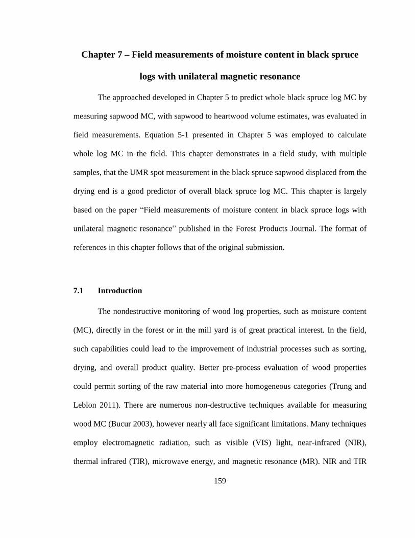
159

Chapter 7 – Field measurements of moisture content in black spruce

logs with unilateral magnetic resonance

The approached developed in Chapter 5 to predict whole black spruce log MC by

measuring sapwood MC, with sapwood to heartwood volume estimates, was evaluated in

field measurements. Equation 5-1 presented in Chapter 5 was employed to calculate

whole log MC in the field. This chapter demonstrates in a field study, with multiple

samples, that the UMR spot measurement in the black spruce sapwood displaced from the

drying end is a good predictor of overall black spruce log MC. This chapter is largely

based on the paper “Field measurements of moisture content in black spruce logs with

unilateral magnetic resonance” published in the Forest Products Journal. The format of

references in this chapter follows that of the original submission.

7.1 Introduction

The nondestructive monitoring of wood log properties, such as moisture content

(MC), directly in the forest or in the mill yard is of great practical interest. In the field,

such capabilities could lead to the improvement of industrial processes such as sorting,

drying, and overall product quality. Better pre-process evaluation of wood properties

could permit sorting of the raw material into more homogeneous categories (Trung and

Leblon 2011). There are numerous non-destructive techniques available for measuring

wood MC (Bucur 2003), however nearly all face significant limitations. Many techniques

employ electromagnetic radiation, such as visible (VIS) light, near-infrared (NIR),

thermal infrared (TIR), microwave energy, and magnetic resonance (MR). NIR and TIR

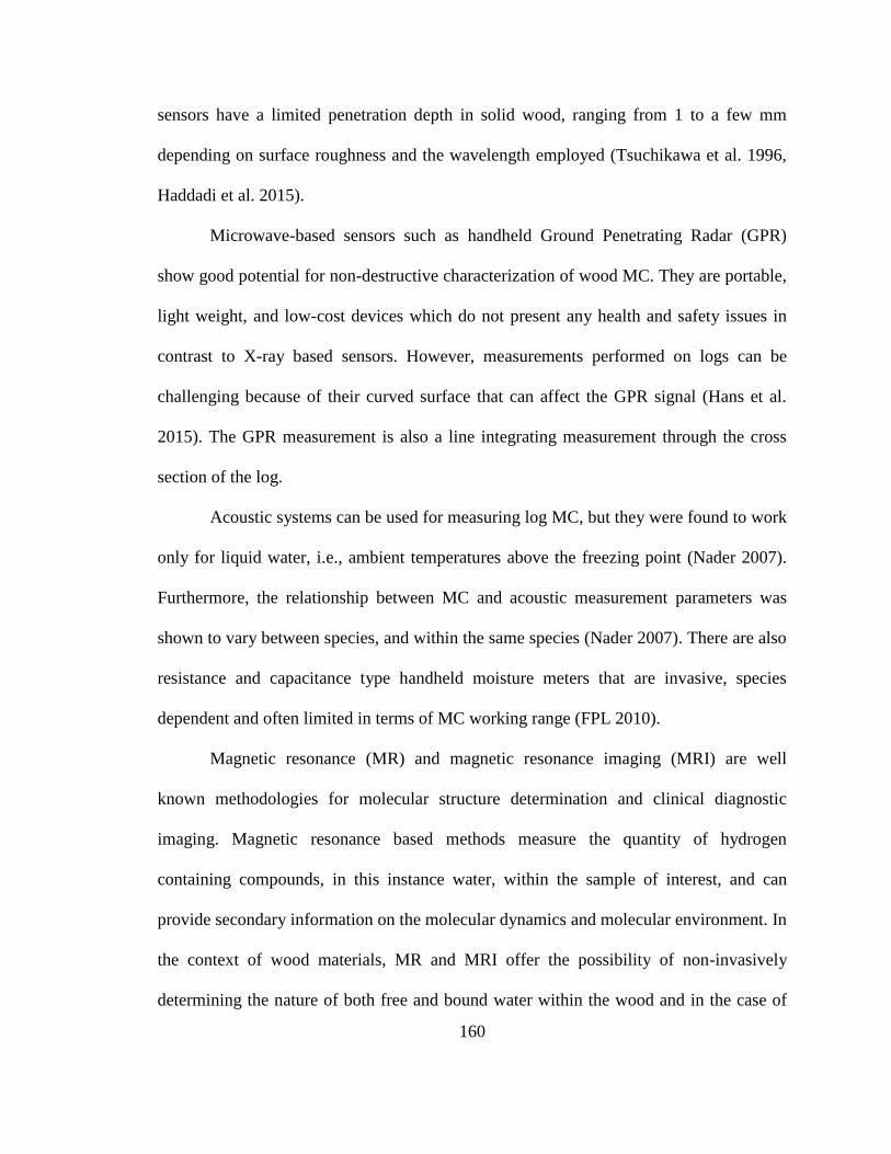
160

sensors have a limited penetration depth in solid wood, ranging from 1 to a few mm

depending on surface roughness and the wavelength employed (Tsuchikawa et al. 1996,

Haddadi et al. 2015).

Microwave-based sensors such as handheld Ground Penetrating Radar (GPR)

show good potential for non-destructive characterization of wood MC. They are portable,

light weight, and low-cost devices which do not present any health and safety issues in

contrast to X-ray based sensors. However, measurements performed on logs can be

challenging because of their curved surface that can affect the GPR signal (Hans et al.

2015). The GPR measurement is also a line integrating measurement through the cross

section of the log.

Acoustic systems can be used for measuring log MC, but they were found to work

only for liquid water, i.e., ambient temperatures above the freezing point (Nader 2007).

Furthermore, the relationship between MC and acoustic measurement parameters was

shown to vary between species, and within the same species (Nader 2007). There are also

resistance and capacitance type handheld moisture meters that are invasive, species

dependent and often limited in terms of MC working range (FPL 2010).

Magnetic resonance (MR) and magnetic resonance imaging (MRI) are well

known methodologies for molecular structure determination and clinical diagnostic

imaging. Magnetic resonance based methods measure the quantity of hydrogen

containing compounds, in this instance water, within the sample of interest, and can

provide secondary information on the molecular dynamics and molecular environment. In

the context of wood materials, MR and MRI offer the possibility of non-invasively

determining the nature of both free and bound water within the wood and in the case of

161

MRI allowing water concentration spatially resolved (Araujo 1993; Casieri et al. 2004;

Lamason et al. 2014, 2015; MacMillan et al. 2002, 2011). The water in the sample must

not be frozen as shown in Lamason et al. (2014). The MR signal lifetimes of frozen water

do not permit MRI.

A promising recent development in MR is the advancement of portable unilateral

magnetic resonance (UMR). Numerous studies and designs have been presented in the

literature. Blümich et al. (2005 and 2008) presented a review on the advances of single-

sided MR. Unilateral magnetic resonance has been employed in many different

measurement problems. In food and agriculture research, Veliyulin et al. (2008)

employed UMR for rapid and non-destructive determination of fat content in dairy

products. Other applications include biomedicine, polymers, cultural heritage, porous

media and building materials (Blümich et al. 2008).

There are relatively few studies in the literature which employ portable UMR

sensors for wood measurement. Casieri et al. (2004) employed portable UMR as a non-

destructive and non-invasive tool for water content analysis and moisture fraction

determination in wood. Senni et al. (2009) employed a portable UMR sensor for in situ

non-invasive determination of MC of wooden works of art and painted wood. Portable

UMR was employed by Dvinskikh et al. (2011) to study MC profiles and water uptake


properties of a wood coating with a portable UMR sensor. Most sensors employed have a

maximum depth of penetration of 3-5 mm. Lamason et al. (2014) employed a UMR

sensor that has a penetration depth of 13 mm to observe freeze/thaw behavior of wood

samples.

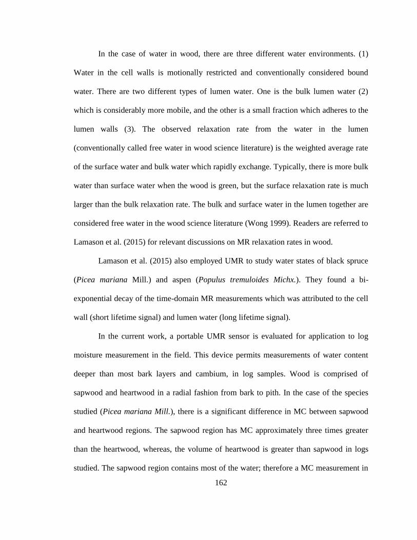
162



water. There are two different types of lumen water. One is the bulk lumen water (2)



(conventionally called free water in wood science literature) is the weighted average rate

of the surface water and bulk water which rapidly exchange. Typically, there is more bulk

water than surface water when the wood is green, but the surface relaxation rate is much

larger than the bulk relaxation rate. The bulk and surface water in the lumen together are

considered free water in the wood science literature (Wong 1999). Readers are referred to

Lamason et al. (2015) for relevant discussions on MR relaxation rates in wood.

Lamason et al. (2015) also employed UMR to study water states of black spruce

(Picea mariana Mill.) and aspen (Populus tremuloides Michx.). They found a bi-

exponential decay of the time-domain MR measurements which was attributed to the cell

wall (short lifetime signal) and lumen water (long lifetime signal).

In the current work, a portable UMR sensor is evaluated for application to log

moisture measurement in the field. This device permits measurements of water content

deeper than most bark layers and cambium, in log samples. Wood is comprised of

sapwood and heartwood in a radial fashion from bark to pith. In the case of the species

studied (Picea mariana Mill.), there is a significant difference in MC between sapwood

and heartwood regions. The sapwood region has MC approximately three times greater

than the heartwood, whereas, the volume of heartwood is greater than sapwood in logs

studied. The sapwood region contains most of the water; therefore a MC measurement in

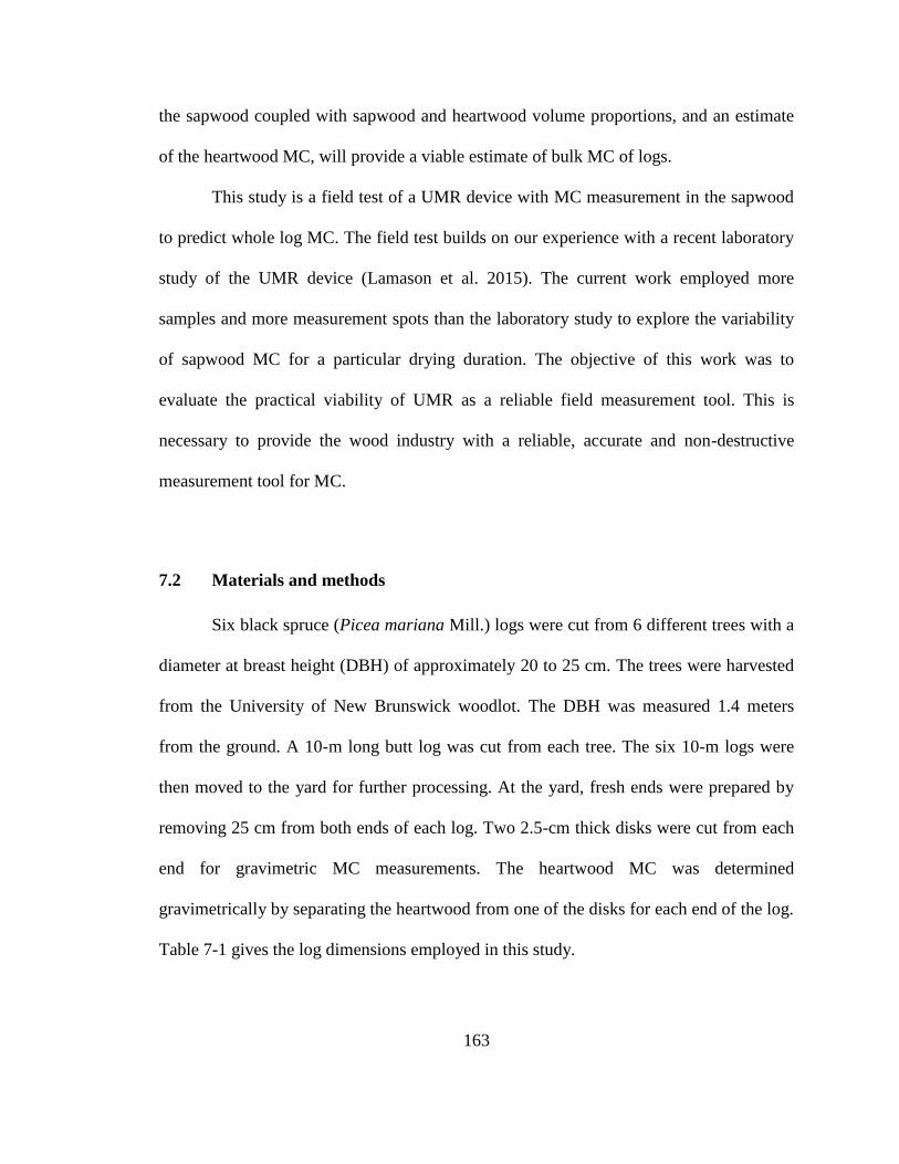
163

the sapwood coupled with sapwood and heartwood volume proportions, and an estimate

of the heartwood MC, will provide a viable estimate of bulk MC of logs.

This study is a field test of a UMR device with MC measurement in the sapwood

to predict whole log MC. The field test builds on our experience with a recent laboratory

study of the UMR device (Lamason et al. 2015). The current work employed more

samples and more measurement spots than the laboratory study to explore the variability

of sapwood MC for a particular drying duration. The objective of this work was to

evaluate the practical viability of UMR as a reliable field measurement tool. This is

necessary to provide the wood industry with a reliable, accurate and non-destructive

measurement tool for MC.


Six black spruce (Picea mariana Mill.) logs were cut from 6 different trees with a

diameter at breast height (DBH) of approximately 20 to 25 cm. The trees were harvested

from the University of New Brunswick woodlot. The DBH was measured 1.4 meters

from the ground. A 10-m long butt log was cut from each tree. The six 10-m logs were

then moved to the yard for further processing. At the yard, fresh ends were prepared by

removing 25 cm from both ends of each log. Two 2.5-cm thick disks were cut from each

end for gravimetric MC measurements. The heartwood MC was determined

gravimetrically by separating the heartwood from one of the disks for each end of the log.

Table 7-1 gives the log dimensions employed in this study.

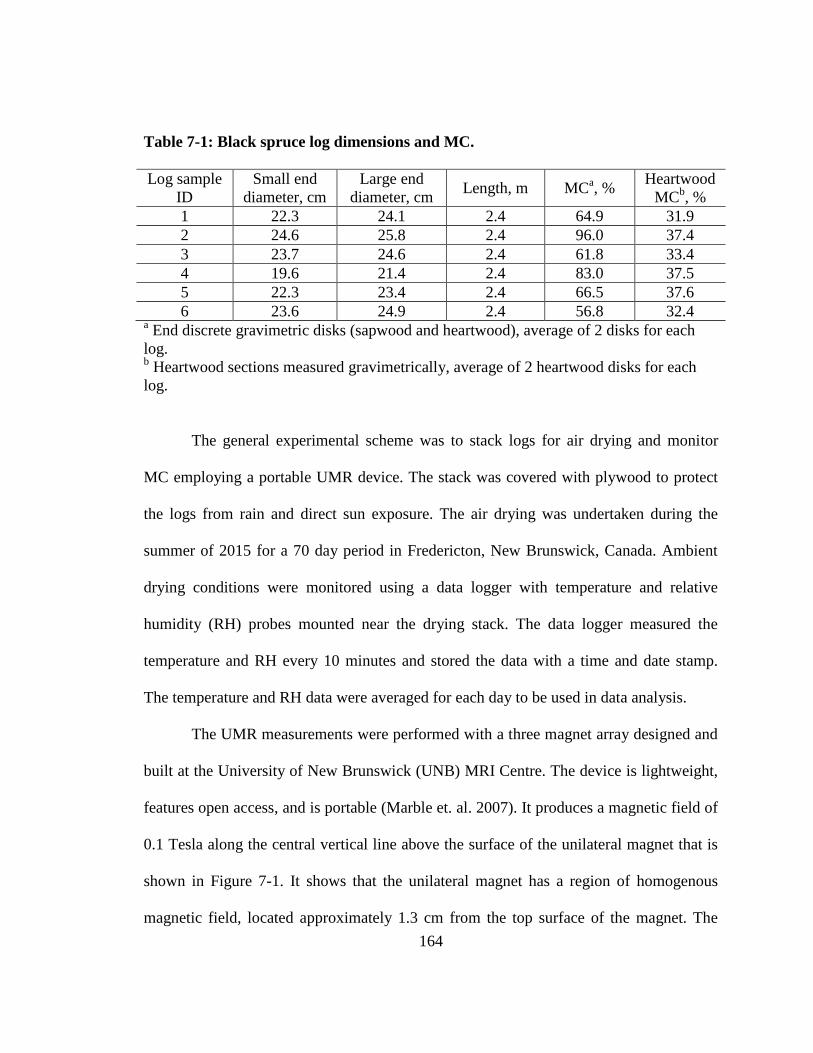
164

Table 7-1: Black spruce log dimensions and MC.

Log sample

ID

Small end

diameter, cm

Large end

diameter, cm Length, m MC

a, %

Heartwood

MCb, %

1 22.3 24.1 2.4 64.9 31.9

2 24.6 25.8 2.4 96.0 37.4

3 23.7 24.6 2.4 61.8 33.4

4 19.6 21.4 2.4 83.0 37.5

5 22.3 23.4 2.4 66.5 37.6

6 23.6 24.9 2.4 56.8 32.4 a End discrete gravimetric disks (sapwood and heartwood), average of 2 disks for each

log. b Heartwood sections measured gravimetrically, average of 2 heartwood disks for each

log.

The general experimental scheme was to stack logs for air drying and monitor

MC employing a portable UMR device. The stack was covered with plywood to protect

the logs from rain and direct sun exposure. The air drying was undertaken during the

summer of 2015 for a 70 day period in Fredericton, New Brunswick, Canada. Ambient

drying conditions were monitored using a data logger with temperature and relative

humidity (RH) probes mounted near the drying stack. The data logger measured the

temperature and RH every 10 minutes and stored the data with a time and date stamp.

The temperature and RH data were averaged for each day to be used in data analysis.

The UMR measurements were performed with a three magnet array designed and

built at the University of New Brunswick (UNB) MRI Centre. The device is lightweight,

features open access, and is portable (Marble et. al. 2007). It produces a magnetic field of

0.1 Tesla along the central vertical line above the surface of the unilateral magnet that is

shown in Figure 7-1. It shows that the unilateral magnet has a region of homogenous

magnetic field, located approximately 1.3 cm from the top surface of the magnet. The

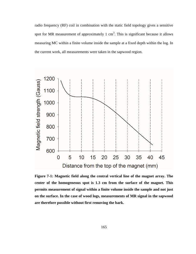
165

radio frequency (RF) coil in combination with the static field topology gives a sensitive

spot for MR measurement of approximately 1 cm3. This is significant because it allows

measuring MC within a finite volume inside the sample at a fixed depth within the log. In

the current work, all measurements were taken in the sapwood region.

Figure 7-1: Magnetic field along the central vertical line of the magnet array. The


permits measurement of signal within a finite volume inside the sample and not just

on the surface. In the case of wood logs, measurements of MR signal in the sapwood

are therefore possible without first removing the bark.

166

The unilateral magnet RF probe was connected to a quarter lambda circuit. A

Tomco RF amplifier (BT00250-AlphaS, Tomco Technologies, Adelaide, Australia),

Tecmag LapNMR console (Tecmag, Houston, Tx, USA) and acquisition laptop were

employed in the field measurements. The MR frequency in the sensitive spot was 4.46

MHz. The UMR measurements were performed employing a Carr-Purcell-Meiboom-Gill

(CPMG) measurement to determine the transverse relaxation time T2 and signal

amplitude. The initial MR signal amplitude was proportional to MC. CPMG

measurement parameters were: echo time = 160 µs, scans = 512, and number of echoes =

1024. The 180° pulse length, 11 µs, and the 90° pulse length were the same but the 90°

pulse power was 6 dB attenuated with respect to the 180° pulse. The overall acquisition

time for each chosen spot was approximately 10 min. The UMR sensor was in direct

contact with the log surface throughout the measurement.

For each spot measurement, a reference sample was first measured, followed by

logs 1, 2 and 3. The reference sample had 30% MC and was fabricated from a mix of

H2O, deuterium oxide (D2O), and copper sulfate. The reference sample was then re-

measured to ensure instrument and measurement stability. Measurements of logs 4, 5 and

6 commenced after re-measuring the reference sample.

The UMR measurements were undertaken at 4 different spots in the sapwood,

through the bark, for each log. The four spots were located 15 cm from the bottom of the

log and were evenly spaced around the circumference at 90 degree intervals. Two

perpendicular lines were inscribed at the end of each log to ensure consistent orientation

during measurements. The measurement spots were carefully marked to maintain the

same spot for succeeding UMR measurements. Data from the 4 spots provided

167

information about the variability of MC in sapwood at this chosen distance from the end.

Variability in sapwood MC was examined throughout the duration of drying in the field.

Apart from the 4 measurement spots displaced 15 cm from the end, measurements at the

midpoint longitudinally were undertaken for three of the six logs. In practice, it was

sometimes difficult to access the midpoint of the log especially in logs that are placed in

the interior of the stack.

The CPMG decays were analyzed using bi-exponential fitting, performed with a

least-squared regression in SigmaPlot (Systat Software Inc., USA). The CPMG decay

constant is the T2 relaxation time. A bi-exponential fitting permits determination of the

relative water content in different environments (cell wall and lumen), based on the

lifetime of the MR signal. The short lifetime signal component is related to the cell wall

water, while the long lifetime signal component is related to the lumen water (Riggin et

al. 1979; Menon et al. 1987 and 1989; Lamason et al. 2015). The sum of the two signal

populations are converted into MCs by employing a reference sample of known MC.


Figure 7-2 shows photos taken during the field measurements. Logs were stacked

outside and individual logs were moved and placed on a work bench under cover during

UMR measurements. Figure 7-3 shows the average daily temperature and relative

humidity near the drying stack. The average daily air drying temperature and relative

humidity ranged from 14.9 to 24.8 °C and 57.6 to 93.9%, respectively.

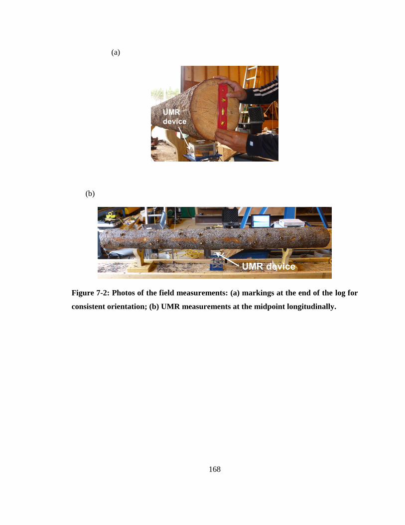
168

(a)

(b)

Figure 7-2: Photos of the field measurements: (a) markings at the end of the log for

consistent orientation; (b) UMR measurements at the midpoint longitudinally.

169

Figure 7-3: Average daily temperature and relative humidity near the drying stack.

Typically, when wood is wet (green condition) the signal intensity measured with

the UMR in a CPMG measurement decayed bi-exponentially (Lamason et al. 2015). The

short lifetime signal component, for freshly cut black spruce sapwood, is associated with

the water in the cell walls while the long lifetime signal component is associated with the

lumen water (Riggin et al. 1979; Menon et al. 1987 and 1989; Araujo et al. 1992;

Lamason et al. 2015). The bi-exponential fitting employed was sufficient to fit the

experimental decay. Previous work on spin-spin relaxation rates in porous media, such as

wood, suggests that MR measurement could differentiate water in three different cell

sizes. However, there was no experimental evidence of three discrete exponentials in the

current work. Menon et al. (1987 and 1989) assigned earlywood and latewood lumen

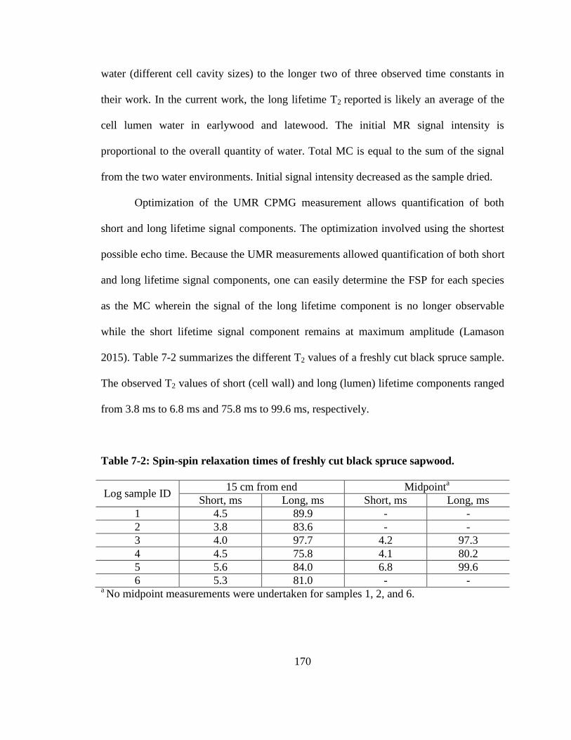
170

water (different cell cavity sizes) to the longer two of three observed time constants in

their work. In the current work, the long lifetime T2 reported is likely an average of the

cell lumen water in earlywood and latewood. The initial MR signal intensity is

proportional to the overall quantity of water. Total MC is equal to the sum of the signal

from the two water environments. Initial signal intensity decreased as the sample dried.

Optimization of the UMR CPMG measurement allows quantification of both

short and long lifetime signal components. The optimization involved using the shortest

possible echo time. Because the UMR measurements allowed quantification of both short

and long lifetime signal components, one can easily determine the FSP for each species

as the MC wherein the signal of the long lifetime component is no longer observable

while the short lifetime signal component remains at maximum amplitude (Lamason

2015). Table 7-2 summarizes the different T2 values of a freshly cut black spruce sample.

The observed T2 values of short (cell wall) and long (lumen) lifetime components ranged

from 3.8 ms to 6.8 ms and 75.8 ms to 99.6 ms, respectively.

Table 7-2: Spin-spin relaxation times of freshly cut black spruce sapwood.

Log sample ID 15 cm from end Midpoint

a

Short, ms Long, ms Short, ms Long, ms

1 4.5 89.9 - -

2 3.8 83.6 - -

3 4.0 97.7 4.2 97.3

4 4.5 75.8 4.1 80.2

5 5.6 84.0 6.8 99.6

6 5.3 81.0 - - a No midpoint measurements were undertaken for samples 1, 2, and 6.

171

Figure 7-4 plots the total water as a function of drying time in sapwood in a

measurement spot 15 cm from the end of the log, through the bark. Each data point was

the average value of the 4 different spots for each individual log (Fig 7-4a-f). Overall, the

total signal decreases with air drying duration. The total signal intensity in the sapwood

did not significantly change in the early stages of drying. However, for all samples, there

was a significant drop in the signal intensity at 70 days of drying. This was due to the fact

that the end drying front has reached the measurement spot during this stage of drying.

Variability in the data among the 4 spots increased with drying time. Variability was also

observed between samples. As the drying front progresses into the log, some

measurement spots will be drier than others for a particular drying duration.

The signal to noise ratio (SNR) was calculated as the ratio of maximum signal

amplitude and standard deviation in the noise level. It was found that the SNR decreased

by a factor of 10 from Day 1 to Day 70. The typical SNR at the initial condition was

approximately 100. The decrease in SNR as drying time progressed is attributed to the

decrease of MR signal as MC of the sample decreases. The noise level remained constant.

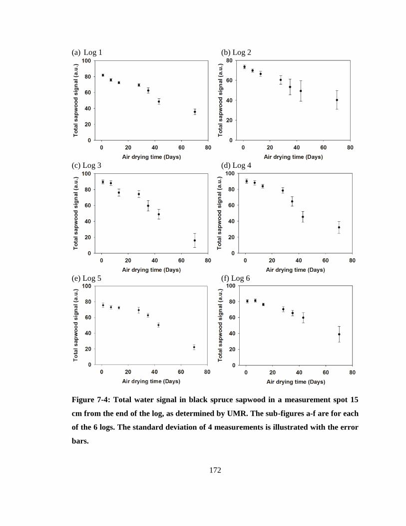
172

(a) Log 1 (b) Log 2

(c) Log 3 (d) Log 4

(e) Log 5 (f) Log 6

Figure 7-4: Total water signal in black spruce sapwood in a measurement spot 15

cm from the end of the log, as determined by UMR. The sub-figures a-f are for each

of the 6 logs. The standard deviation of 4 measurements is illustrated with the error

bars.

173

Figure 7-5 plots the total water signal as a function of drying time in sapwood at

the midpoint longitudinally in three logs. The total signal intensity in the sapwood

decreases with air drying duration. The signal intensity at 70 days of drying was less than

that of the early stages of drying. The signal intensity at the midpoint longitudinally is

higher than the signal intensity at 15 cm from the end of the log at the same drying

duration. This suggests that the diffusive drying front, from the exposed end, has reached

the 15 cm measurement spot during this time. The R2 values of the best fit line for logs 3,

4 and 5 were 0.87, 0.94 and 0.79, respectively.

The total sapwood signal intensities were converted to MC using a standardized

reference sample with known MC. Only data from one of the three logs in Figure 7-5 are

presented. This result is however representative of the findings for all 3 logs measured at

the midpoint longitudinally. Figure 7-6 (data for log 3 only) shows that the measured

sapwood MC in a spot 15 cm from the end (Fig.6a), and at the midpoint longitudinally

(Fig. 7-6b) were linearly related to the gravimetric MC of the whole log sample. The

relationship is clear especially during early stages of air drying. This is due to the fact

that most of the water loss occurred in the sapwood and that the observed diffusive

drying at the end surfaces of the log does not significantly affect the overall MC during

early stages of drying. The exact position of the measured spot does not matter as long as

it is displaced from the ends. The UMR measurements in Figure 7-6 were undertaken at

air drying times which ranged from one to seventy days.

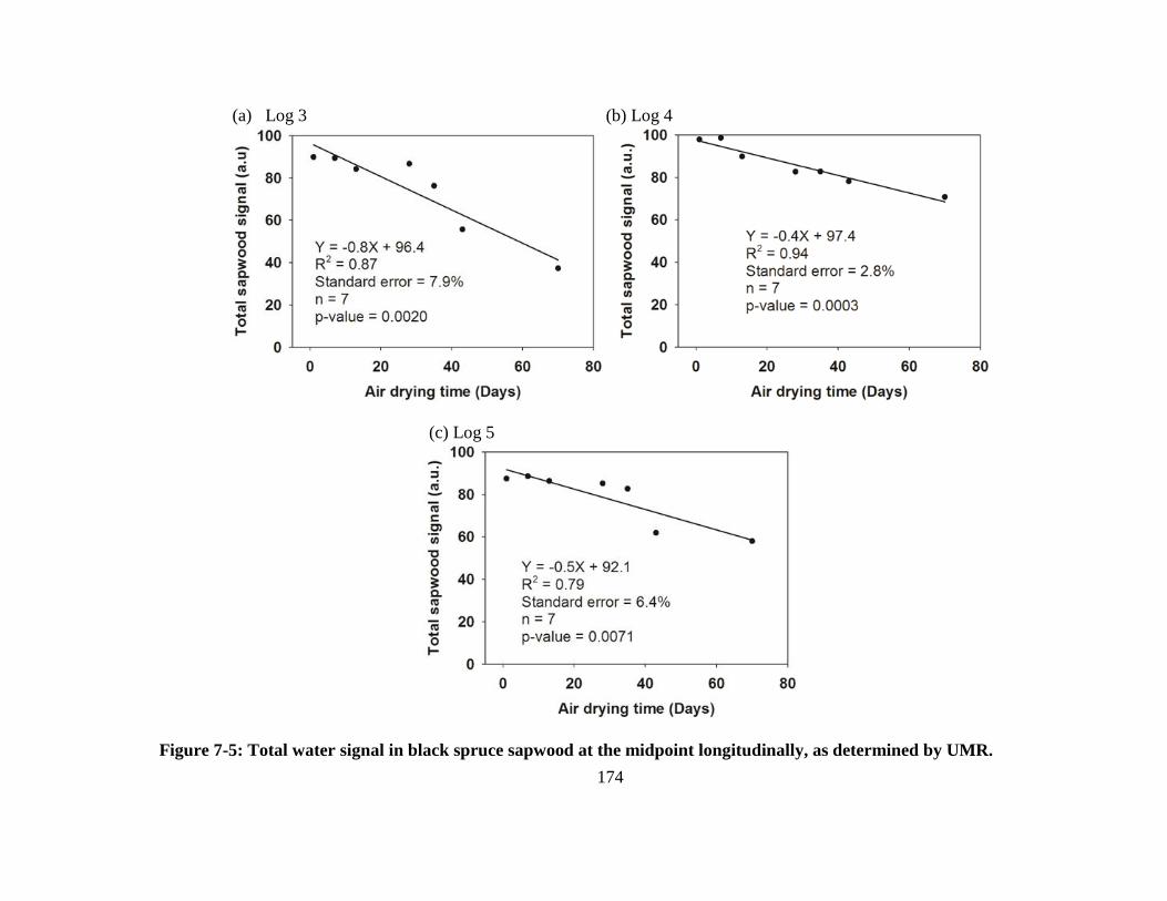
174

(a) Log 3 (b) Log 4

(c) Log 5

Figure 7-5: Total water signal in black spruce sapwood at the midpoint longitudinally, as determined by UMR.

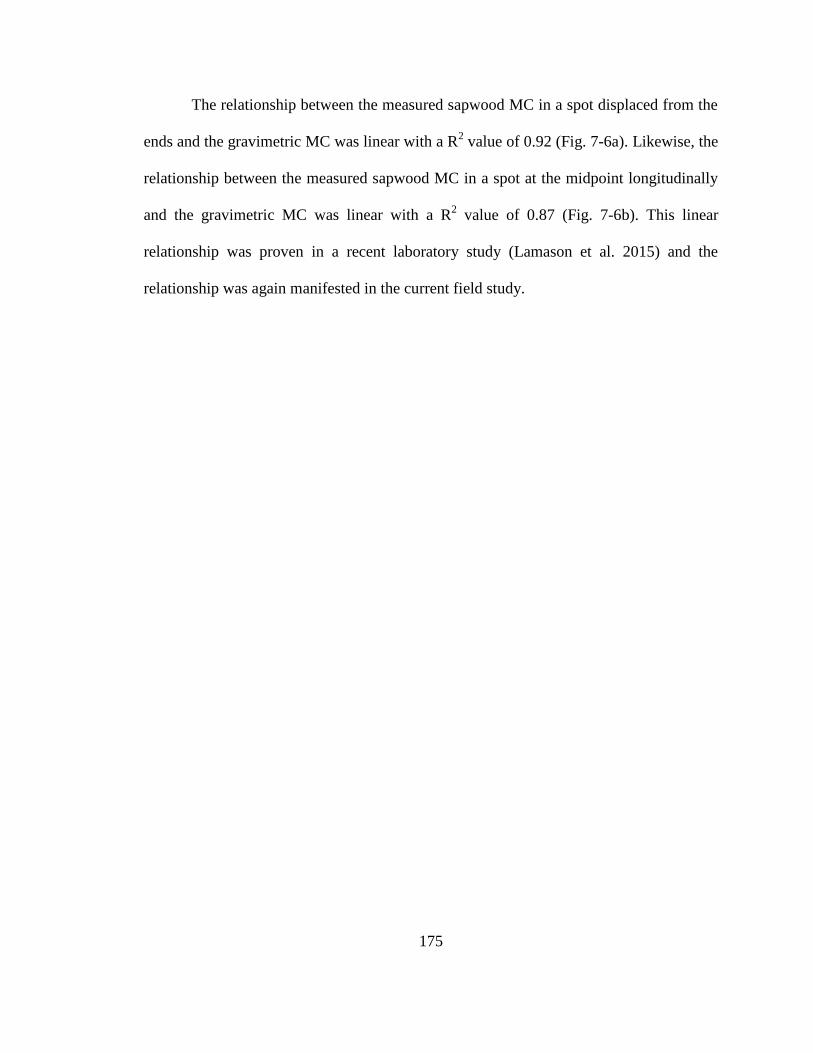
175

The relationship between the measured sapwood MC in a spot displaced from the

ends and the gravimetric MC was linear with a R2 value of 0.92 (Fig. 7-6a). Likewise, the

relationship between the measured sapwood MC in a spot at the midpoint longitudinally

and the gravimetric MC was linear with a R2 value of 0.87 (Fig. 7-6b). This linear

relationship was proven in a recent laboratory study (Lamason et al. 2015) and the

relationship was again manifested in the current field study.

176

(a) 15 cm from the end

(b) Midpoint

Figure 7-6: Linear relationship between sapwood MC in a spot 15 cm from the end

(a) and at the midpoint longitudinally (b) to that of the overall log gravimetric MC

in the case of Log 3.

177

The boundary between sapwood and heartwood was visually determined by

observing the difference in color and transparency at the cut end. There is a large visual

disparity between heartwood and sapwood MC. The sapwood area was estimated by

subtracting bark area and heartwood area from the total cross-sectional stem area. For

these samples, the sapwood thickness was approximately 1.8 cm and the ratio of sapwood

to heartwood was 25:75 with respect to the overall volume of the log. It was assumed that

the log was cylindrical and that heartwood MC does not change significantly unless the

MC of sapwood is at or near FSP.

A reliable estimation of MC of logs includes a direct MC measurement of

sapwood and takes into account the volume proportions of the heartwood and sapwood

regions as well as an estimate of heartwood MC assumed in the case of black spruce to be

at FSP. One difficulty with this approach is that not all species of wood have a distinct

boundary between sapwood and heartwood. For species with a clear distinction between

heartwood and sapwood, a simple measurement approach as described by equation 7-1

may be employed.

𝑀𝐶𝑙𝑜𝑔 = (𝑀𝐶𝑠𝑎𝑝𝑤𝑜𝑜𝑑 × % 𝑉𝑜𝑙𝑠𝑎𝑝𝑤𝑜𝑜𝑑) + (𝑀𝐶ℎ𝑒𝑎𝑟𝑡𝑤𝑜𝑜𝑑 × % 𝑉𝑜𝑙ℎ𝑒𝑎𝑟𝑡𝑤𝑜𝑜𝑑) (Eqn 7-1)

where MClog is the overall MC of the log. MCsapwood and % Volsapwood are moisture

content and volume proportion of sapwood to the entire volume of the log, respectively.

MCheartwood and % Volheartwood correspond to moisture content and volume proportion of

heartwood to the entire volume of the log. The first term in equation 7-1 was measured

and the remaining terms were estimated assuming the heartwood is at fiber saturation

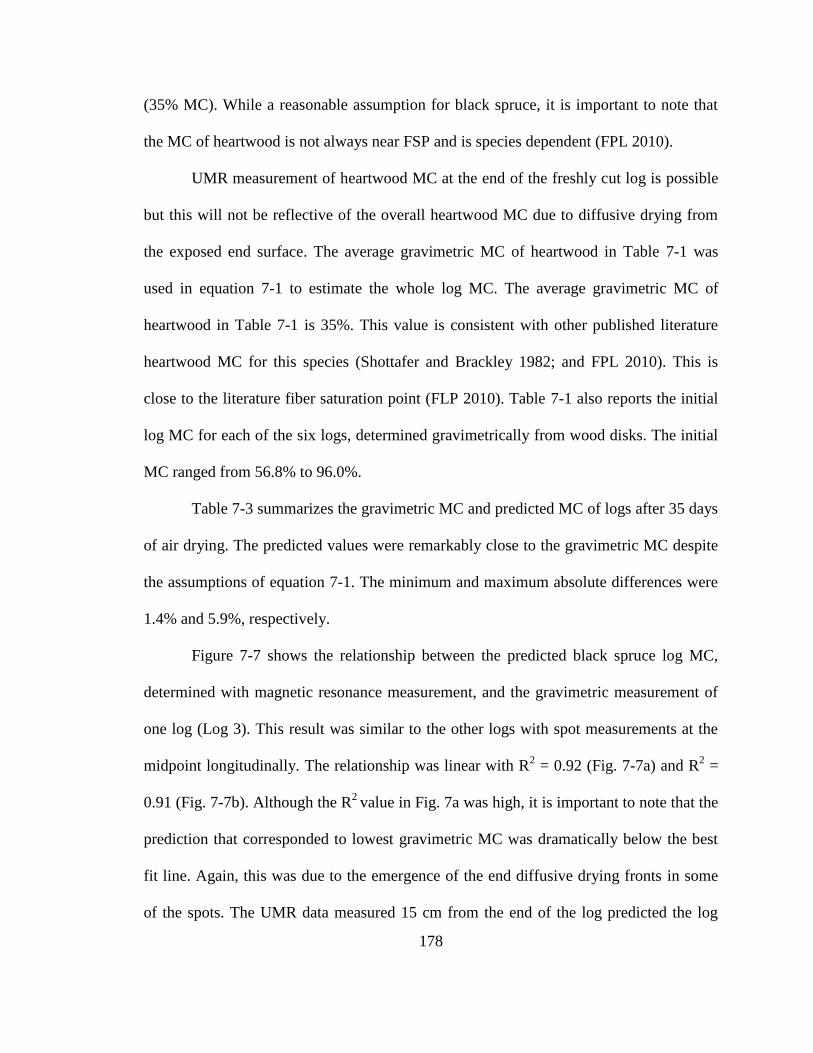
178

(35% MC). While a reasonable assumption for black spruce, it is important to note that

the MC of heartwood is not always near FSP and is species dependent (FPL 2010).

UMR measurement of heartwood MC at the end of the freshly cut log is possible

but this will not be reflective of the overall heartwood MC due to diffusive drying from

the exposed end surface. The average gravimetric MC of heartwood in Table 7-1 was

used in equation 7-1 to estimate the whole log MC. The average gravimetric MC of

heartwood in Table 7-1 is 35%. This value is consistent with other published literature

heartwood MC for this species (Shottafer and Brackley 1982; and FPL 2010). This is

close to the literature fiber saturation point (FLP 2010). Table 7-1 also reports the initial

log MC for each of the six logs, determined gravimetrically from wood disks. The initial

MC ranged from 56.8% to 96.0%.

Table 7-3 summarizes the gravimetric MC and predicted MC of logs after 35 days

of air drying. The predicted values were remarkably close to the gravimetric MC despite

the assumptions of equation 7-1. The minimum and maximum absolute differences were

1.4% and 5.9%, respectively.

Figure 7-7 shows the relationship between the predicted black spruce log MC,

determined with magnetic resonance measurement, and the gravimetric measurement of

one log (Log 3). This result was similar to the other logs with spot measurements at the

midpoint longitudinally. The relationship was linear with R2 = 0.92 (Fig. 7-7a) and R

2 =

0.91 (Fig. 7-7b). Although the R2

value in Fig. 7a was high, it is important to note that the

prediction that corresponded to lowest gravimetric MC was dramatically below the best

fit line. Again, this was due to the emergence of the end diffusive drying fronts in some

of the spots. The UMR data measured 15 cm from the end of the log predicted the log

179

MC well especially during early stages of drying. The challenge occurred when the

diffusive end drying advanced sufficiently longitudinally so that the UMR signal at any

of the end spots is not representative of the sapwood MC in the log. In this case the UMR

signal amplitude is no longer predictive of the bulk (gravimetric) MC of the log as

suggested in Equation 7-1.The relationship between the predicted black spruce log MC,

determined with magnetic resonance measurement, and the gravimetric measurement was

linear. The UMR derived MC has an estimated uncertainty, in absolute MC, of 2.6%

(Fig. 7-7a) and 2.2% (Fig. 7-7b). This measurement approach is a viable strategy in

predicting MC of black spruce logs in the field.

Table 7-3: List of gravimetric and predicted MC of each log at 35 days of air drying.

The predicted MC involves estimation of sapwood and heartwood volume

proportions.

Log sample ID Gravimetric MC, % Predicted MC, % Absolute difference,

%

1 59.0 53.1 5.9

2 86.1 82.0 4.1

3 54.8 51.4 3.4

4 74.7 73.3 1.4

5 59.8 55.2 4.6

6 51.1 45.4 5.7

180

(a) 15 cm from the end

(b) Midpoint

Figure 7-7: Linear relationship between MC predicted by magnetic resonance

measurement plotted versus MC determined gravimetrically in the case of Log 3.

The UMR measurement of sapwood MC was scaled through the heartwood and

sapwood volume proportions to yield a whole sample estimate. The different MCs

correspond to different drying times, specifically 1, 7, 13, 28, 35, 43 and 70 days. The

diffusive end drying reaches the spot 15 cm from the end (a) at the later stage of

drying. The better location when accessible is at the midpoint longitudinally (b).

181

7.3 Conclusions

The UMR spot estimates of bulk MC in the sapwood can be used to estimate the

overall MC of a black spruce log in the field. The sapwood measured MC coupled with

sapwood to heartwood proportions is a viable approach to predicting log MC. The

unilateral magnetic resonance method will allow measurement of water in samples that

are not debarked as it measures a volume located 1.3 cm below the surface, which is a

significant operational advantage.

MC variability of the measurement spots displaced from the end increased as

drying progresses. Despite this variability, both the spot at the midpoint longitudinally,

and the spot displaced from the ends gave predictions that were remarkably close to the

gravimetric MC. A ‘through the bark’ measurement is ideal, especially if the device is

able to directly measure sapwood.

The use of a portable unilateral magnetic resonance instrument to measure MC in

wood log samples was demonstrated. This instrument has the advantage of portability,

permitting MC estimations of thawed logs in the field without oven drying. One may

anticipate that further development will lead to a reduction in the acquisition time as

measurement hardware and software improves.

182

7.4 References

Araujo, C.D. 1993. Proton magnetic resonance of wood and water in wood. Dissertation,

University of British Columbia.

Blümich, B., F. Casanova, J. Perlo, S. Anferova, V. Anferov, K. Kremer, N. Goga, K.

Kupferschlager, and M. Adams. 2005. Advances of unilateral mobile NMR in

non-destructive materials testing. Magn. Reson. Imaging 23(2):197-201.

Blümich, B., J. Perlo, and F. Casanova. 2008. Mobile single-sided NMR. Progress in

Nuclear Magnetic Resonance Spectrosc. 52:197-269.

Casieri, C., L. Senni, M. Romagnoli, U. Santamaria, and F. DeLuca. 2004. Determination

of moisture fraction in wood by mobile NMR device. J. Magn. Reson.

171(2):364-372.

Dvinskikh, S. V., I. Furo, D. Sandberg, and O. Soderstrom. 2011. Moisture content

profiles and uptake kinetics in wood cladding materials evaluated by a portable

nuclear magnetic resonance spectrometer. Wood Mater. Sci. Eng. 6:119-127.

Hans, G., D. Redman, B. Leblon, J. Nader, and A. La Rocque. 2015. Determination of

log moisture content using ground penetrating radar (GPR). Part 1. Partial least

squares (PLS) method. Holzforschung. doi:10.1515/hf-2014-0286.

FPL. 2010. Wood handbook – Wood as an engineering material. Gen Tech Rep FPL-


Lamason, C., B. MacMillan, B. J. Balcom, B. Leblon, and Z. Pirouz. 2014. Examination

of water phase transitions in black spruce by magnetic resonance and magnetic

resonance imaging. Wood and Fiber Sci 46(4):1-14. (also Chapter 3 of this

Thesis)

Lamason, C., B. MacMillan, B. J. Balcom, B. Leblon, and Z. Pirouz. 2015. Water content


magnetic resonance devices. Wood Mater. Sci. Eng. 10(1):86-93. (also Chapter 4

of this Thesis)

MacMillan, B., M. H. Schneider, A. R. Sharp, and B. J. Balcom. 2002. Magnetic

resonance imaging of water concentration in low moisture content wood. Wood

Fiber Sci. 2:276-286.

MacMillan, B., E. Veliyulin, C. Lamason, and B. J. Balcom. 2011. Quantitative magnetic

resonance measurements of low moisture content wood. Can. J. For. Res.

41:2158-2162.

183

Marble, A. E., I. V. Mastikhin, B. G. Colpitts, and B. J. Balcom. 2007. A compact

permanent magnet array with a remote homogenous field. J. Magn. Reson 186

(1):100-104.

Menon, R. S., A. L. MacKay, J. R. T. Hailey, M. Bloom, A. E. Burgess, and J. S.

Swanson. 1987. An NMR determination of the physiological water distribution in

wood during drying. J. Appl. Polym. Sci. 33:1141-1155.

Menon, R. S., A. L. MacKay, S. Flibotte, and J. R. T. Hailey. 1989. Quantitative

separation of NMR images of water in wood on the basis of T2. J. Magn. Reson

82:205-210.

Nader, J. 2007. Evaluation of two technologies to determine the moisture content of logs.

FPInnovations, Pointe-Claire, QC, Canada.

Pourmand, P., L. Wang, and S. V. Dvinskikh. 2011. Assessment of moisture protective

properties of wood coatings by a portable NMR sensor. J. Coat. Technol. Res.

8(5):649-654.

Riggin, M. T., A. R. Sharp, and R. Kaiser, 1979. Transverse NMR relaxation of water in

wood. J. Apl. Pol. Sci. 23(11):3147-3154.

Senni, L., C. Casieri, A. Bovino, and M. C. Gaetani. 2009. A portable NMR sensor for

moisture monitoring of wooden works of art, particularly of paintings on wood.

Wood Sci. Technol. 43:167-180.

Shottafer, J. E., and A. M. Brackley. 1982. An analysis of moisture content variation in

eastern spruce and balsam fir in Maine. Tech. Bulletin No. 104. Life Sciences and

Agriculture Experiment Station. University of Maine, Orono.

Trung, T., and B. Leblon. 2011. The role of sensors in the new forest products industry

and forest bioeconomy. Can. J. For. Res. 41:2097-2099.

Veliyulin, E., I. V. Mastikhin, A. E. Marble, and B. J. Balcom. 2008. Rapid

determination of the fat content in packaged dairy products by unilateral NMR. J.

Sci. Food Agric. 88:2563-2567.

Wong, P. 1999. Methods in the physics of porous media. San Diego, CA: Academic

Press. pp. 337-385.

184

Chapter 8 – Conclusions

This thesis outlines applications of quantitative UMR and MRI measurements for

studies of spatially resolved water content in wood. The theoretical basis of the work was

summarized in Chapter 2 “Wood and Water in Wood”. The experimental studies in the

thesis utilized FID, CPMG, and SPRITE magnetic resonance measurements to determine

water content in wood.

The first experimental study, Chapter 3, was a freeze/thaw study. The use of a

UMR instrument and the SPRITE MRI measurement in a series of thawing and freezing

experiments established the possibility of studying water phase transitions in frozen wood

samples. An abrupt phase transition of free water was observed at -3°C. A more diffuse

phase transition occurred below -60°C which was attributed to a phase change of cell

wall water. The UMR measurement employed allowed determination of relative

quantities of cell wall and lumen water in wood. None of the MR and MRI measurements

undertaken were able to measure frozen water. Therefore, MR and MRI measurements of

frozen samples do not permit an estimation of the amount of frozen water. This is true for

small laboratory samples and for log samples in the field.

The subsequent chapter, Chapter 4, demonstrated that MR is a powerful tool for

distinguishing water states in wood through measurements of spin-spin relaxation times.

The water content and water behavior in wood materials change with drying. The MR

relaxation times decrease as moisture content decreases. At moisture contents above the

fiber saturation point, water resides in two distinct environments. Lumen water was

removed first while drying above FSP. The amount of cell wall water does not change

185

significantly above 40% MC. No signal from lumen water was observed at or below 20%

MC. In addition, we demonstrated the use of a portable UMR instrument as a powerful

tool in monitoring and estimating MC in wood samples as long as the MC is above the

FSP. This instrument has the advantage of portability, permitting moisture content

estimations in the field without oven drying. The estimation of MC employing the

unilateral magnet above the FSP agreed well with the gravimetric MC, particularly at

high MCs.

In the next chapters, Chapters 5 and 6, both UMR and SPRITE MRI were

employed to map water in black spruce wood log. Both measurements were employed to

select a position or positions for spot measurements to estimate bulk MC in black spruce

logs. The UMR spot estimates of MC in the sapwood can be used to estimate the overall

MC of the log. The ends and near ends through the bark of the log should be avoided in

estimating MC because of the presence of drying fronts. The drying front can extend

several centimeters from the ends. Surface measurements are not adequate since there is a

wide variation of MC within a sample. A ‘through the bark’ measurement is ideal

because the device was able to directly measure sapwood. Both the UMR and SPRITE

MRI results are in agreement pertaining to the observed drying behavior and MC

estimation. Diffusive end drying and radial drying through the bark was observed. The

effect of radial drying through the bark is more significant compared to the diffusive end

drying even though the diffusive end drying was immediately apparent from Day 1.

The final experimental study was a black spruce field measurement employing the

portable UMR. The sapwood measured MC coupled with sapwood to heartwood

proportions is a viable approach to predicting log MC. The UMR measurement will allow

186

measurement of water in samples that are not debarked as it measures a volume located

1.3 cm below the surface, which is a significant operational advantage. The MC

variability of the measurement spots displaced from the end increased as drying

progresses. Despite this variability, both the spot at the midpoint longitudinally, and at

spots displaced from the ends, gave predictions that were remarkably close to the

gravimetric MC. A ‘through the bark’ measurement is ideal, especially if the device is

able to directly measure sapwood. The thesis has demonstrated the utility of

employing magnetic resonance measurements in the study of water in wood.

In particular, a portable UMR instrument was successfully tested to measure MC

in black spruce wood log samples. A simplified linear model to predict overall log MC

form sapwood MC measured by the UMR in the case of black spruce (Equation 5-1) was

proposed. The model has several assumptions that naturally limit generality of the model.

We first assumed that the heartwood MC is at FSP and much lower than the MC in

sapwood. As a result, the contribution of heartwood MC loss is negligible and most of the

water loss should be in the sapwood. This is the case for black spruce but it may not be

true for other species, particularly hardwoods, where the difference in MC between the

sapwood and heartwood is species-dependent (Table 2.1). It is recommended that other

important wood species be examined in similar studies of log MC estimations.

The proposed approach permits using UMR measurements on logs with bark,

which is an enormous practical advantage. However, black spruce bark is thin enough to

allow UMR measurements reaching the sapwood. This may not be the case for species

having thick bark. Further work is needed to test this approach on logs having thicker

bark.

187

The UMR measurement employed in this thesis was able to differentiate cell wall

and lumen water and to verify that different zones in wood behave differently during

drying. Both are huge advantages compared to other MC measurement techniques.

Indeed, MRI data can help guide new, and improve existing, wood drying models. They

also could be employed to develop better measurement and calibration models for other

moisture content measurement tools currently used in the field.

The cell/lumen water differentiation was done using sensitive spot UMR

measurements. The SPRITE MRI measurement technique was able to image MC in the

wood sample, but only to determine total water. It would be beneficial to wood science

and wood drying research if an MRI technique can be developed to image the different

water states in wood through their difference in relaxation times. Preliminary work has

commenced in the UNB MRI Centre.

The MR measurement is potentially of great importance in improving the forest

industry value chain specifically through monitoring MC. For instance, sorting of logs or

lumber to separate wet from drier wood before processing. In kiln drying operations,

drying a uniform load of lumber would yield a better quality stack by reducing the overall

MC gradient of lumber being dried. In addition, the product quality of plywood and

oriented strand board may be improved by determining MC of logs prior to veneering and

flaking. Logs that are too dry will result in production of too many fines (sawdust) while

a wet log will result in wet veneers and flakes which are too costly to dry to meet product

quality standards.

The MR measurement of MC also has potential to improve wood biomass

production by accurately determining MC in wood residues. This is necessary not only

188

for the optimum pressing conditions of the biomass but also in the overall quality of the

resulting products.

The use of MR in the forest product industry is encouraged by the development of

portable devices such as the UMR device described in this thesis. This instrument has the

advantage of portability, permitting non-destructive, fast and reliable MC estimations of

thawed logs in the field without oven drying. It has therefore the potential of greatly

improving the practicality of MR technology in measuring MC particularly when in the

mill yard.

However, the thesis also showed that they are several challenges associated with

field use of UMR technology in the forest products industry. The UMR magnet must be

kept in a temperature controlled environment to maintain a uniform magnetic field of

constant strength. Also, safety is a critical issue in the forest industry. Extra attention is

required when UMR devices are employed. These devices are sensitive to the presence of

metals. The large attractive forces between the magnets and ferromagnetic metal objects

are potentially very dangerous. Also, the UMR measurement is at present too slow for

practical usage by industry. Further work, both software and hardware is warranted to

speed data acquisition.

189

VITA

Candidate’s full name: Clevan Reyve G. Lamason

Universities attended: University of New Brunswick

Master of Science in Forest Engineering

(2004 – 2006)

University of the Philippines Los Baños

Bachelor of Science in Forest Products Engineering

(1994 – 1999)

Publications:

Lamason C, MacMillan B, Balcom BJ, Leblon B, Pirouz Z (2016) Field measurements of

moisture content in black spruce logs with unilateral magnetic resonance. Forest

Products Journal (doi: 10.13073/FPJ-D-16-00004).

Lamason C, MacMillan B, Balcom BJ, Leblon B, Pirouz Z (2016) Magnetic resonance

studies of wood log-drying processes. Forest Products Journal (doi:

10.13073/FPJ-D-16-00037).



magnetic resonance devices. Wood Material Science and Engineering 10(1):86-

93.



imaging. Wood and Fiber Sci 46(4):1-14.

Lamason C, Viel J, Chui YH (2012) Review of performance requirements for use of

wood siding in mid-rise building applications. Natural Resources Canada’s Value

to Wood Project: UNB11-5.

190


resonance measurements of low moisture content wood. Canadian Journal of

Forest Research 41:2158-2162.

Gong M, Lamason C, and Li L (2010) Interactive effect of surface densification and post

heat-treatment on aspen wood. Journal of Materials Processing Technology

210(2): 293-296.

Lamason C, and Gong M (2007) Optimization of pressing parameters for mechanically

surface-densified aspen. Forest Products Journal 57(10): 64-68.

Gong M, Lamason C (2007) Improvement of surface properties of low density wood:

mechanical modification with heat treatment. Natural Resources Canada’s Value-

to-Wood Project: UNB57.

Conference Presentations:

Lamason C, MacMillan B, Balcom BJ, Leblon B, Pirouz Z (2015) Unilateral magnetic

resonance spot estimates of bulk moisture content in black spruce logs. Poster

Presentation, 13th

International Conference on Magnetic Resonance Microscopy.

August 2-6, Munich, Germany.


phase transitions in black spruce by magnetic resonance. Poster Presentation, 58th

International Society of Wood Science and Technology Convention. June 7-12,

Grand Teton National Park, WY, USA.

Lamason C, MacMillan B, Balcom BJ, Leblon B, Pirouz Z (2015) Water states in black

spruce during drying studied by time-domain magnetic resonance. Poster

Presentation, 58th

International Society of Wood Science and Technology

Convention. June 7-12, Grand Teton National Park, WY, USA.


measurement in black spruce and aspen sapwood with magnetic resonance. Poster

Presentation, 68th

Forest Products Society International Convention, August 10-

13, Quebec, QC, Canada.

Lamason C, MacMillan B, Balcom BJ, Leblon B, Pirouz Z (2013) Log Moisture Content

Determination with Quantitative Magnetic Resonance. Poster Presentation,

Eastern Canadian Section – Forest Products Society Annual General Meeting.

May 29-30, Fredericton, NB, Canada.

191

Lamason C, MacMillan B, Balcom BJ, Leblon B, Pirouz Z (2013) Log moisture content

determination with quantitative magnetic resonance and magnetic resonance

imaging. 18th

International Nondestructive Testing and Evaluation of Wood

Symposium. September 24-27, Madison, WI, USA. pp. 186-195.

Lamason C, Gong M (2007) Improvement of surface properties of aspen by mechanical

densification. Oral Presentation, Forest Products Society 61st International

Convention. Knoxville, Tennessee, USA. June 10-13.

Lamason C, Wang X-M, Chui YH, Chan F (2006) Effect of using spinning-disc atomizer

blender on resin efficiency and board quality. Poster Presentation, Forest Products

Society Meeting, Canada and USA Northeastern Chapter, Delta Hotel,

Fredericton, NB.

Chan F, Darmstadt H, Roy C, de Coumia B, Lamason C, and Chui YH (2004)

Development of Heat-Treated Value-Added Wood Composites. Poster

Presention, 2nd

Eastern CANUSA Forest Science Conference. University of New

Brunswick, Fredericton, New Brunswick. October 15-16.

Lamason C (2003) Alternative sludge management in the Pulp and Paper Industry in the

Philippines. Oral Presentation, National Workshop on Polychlorinated biphenyls

management and alternative sludge management. De La Salle University, Manila,

Philippines. February 28.

Fernandez E, Lamason C, Calderon M, Delgado T (2002) Alternative construction

material from recycling paper mill sludge, in Proceedings 6th

Pacific Rim Bio-

Based Composites Symposium, ed. P. E. Humphrey, Oregon State University,

Corvallis, pp. 177-187.

Fernandez E, Lamason C (2001) Alternative construction material from waste treatment

sludge. Oral presentation, 5th

International Workshop on the Use of Paper

Industry Sludge in Environmental Geo-Technology and Construction. Makati

City, Philippines. May 23-25.

Fernandez E, Lamason C, Delgado T (2000) Cement-bonded boards from wastewater

treatment sludge of a recycled paper mill. Proceedings of a workshop on Wood-

Cement Composites in the Asia-Pacific Region. Canberra, Australia. Ed. P.

Evans, pp. 73-82.

LOG MOISTURE CONTENT DETERMINATION WITH …

Documents

Transcript of LOG MOISTURE CONTENT DETERMINATION WITH …