NBER WORKING PAPER SERIES

LOCATION CHOICE, PORTFOLIO CHOICE

Ioannis BranikasHarrison HongJiangmin Xu

Working Paper 23040http://www.nber.org/papers/w23040

NATIONAL BUREAU OF ECONOMIC RESEARCH1050 Massachusetts Avenue

Cambridge, MA 02138January 2017

We thank Ulrich Mueller, Mark Watson, Chris Sims, Bo Honore, Kirill Evdokimov, Motohiro Yogo, Atif Mian, Jakub Kastl, and participants at Econometrics and Finance seminars at Princeton University, University of Toronto, Johns Hopkins University, 2016 LACEA/LAMES Conference, the 2016 China Five-Star Workshop in Finance, and the 2016 NYU Shanghai Volatility Institute Conference for helpful comments. The views expressed herein are those of the authors and do not necessarily reflect the views of the National Bureau of Economic Research.

NBER working papers are circulated for discussion and comment purposes. They have not been peer-reviewed or been subject to the review by the NBER Board of Directors that accompanies official NBER publications.

© 2017 by Ioannis Branikas, Harrison Hong, and Jiangmin Xu. All rights reserved. Short sections of text, not to exceed two paragraphs, may be quoted without explicit permission provided that full credit, including © notice, is given to the source.

Location Choice, Portfolio ChoiceIoannis Branikas, Harrison Hong, and Jiangmin XuNBER Working Paper No. 23040January 2017JEL No. G02,G11,R2,R22

ABSTRACT

Households hold nondiversified stock portfolios of firms headquartered near their city of residence. Explanations assign a causal role for proximity, either in generating an informational advantage or a familiarity bias. Empirical analyses assume households locate randomly, even though they optimally select a city. This selection is important since latent location factors might be correlated with latent demand for local stocks. Building on location choice models from urban economics, we develop a Heckman (1977)-style model to account for the effect of location choices on portfolio choices. Adjusting for selection significantly reduces local bias and the performance of local stock picks.

Ioannis BranikasEconomics DepartmentPrinceton University Fisher Hall, Room 001Princeton, NJ 08544branikas@princeton.edu

Harrison HongDepartment of EconomicsColumbia University1022 International Affairs BuildingMail Code 3308420 West 118th StreetNew York, NY 10027and NBERhh2679@columbia.edu

Jiangmin XuDepartment of FinanceGuanghua School of ManagementPeking Universityjiangminxu@gsm.pku.edu.cn

1. Introduction

A long-standing puzzle in financial economics is that households hold undiversified stock

portfolios tilted toward firms headquartered near where they reside. Contrary to a value-

weighted market portfolio prescription of the CAPM (Sharpe (1964)), households load on

local stocks regardless of their market value. In canonical regressions of household stock-

portfolio weights on demographic and stock characteristics, distance from household resi-

dence to firm headquarters emerges as a key explanatory variable. This local-bias appears

in many countries.1 This phenomenon is even more puzzling in some ways than its better-

known cousin, the international home-bias puzzle, where households in different countries tilt

toward stocks in their own country (French and Poterba (1991)). In the international setting,

portfolio costs or restrictions at least seem plausible impediments toward diversification.

Given the potentially high costs of under-diversification for households, many theories

have been given for this local bias in the literature.2 There are two influential interpretations

for local bias, and both revolve around the causal role of proximity. The first is that prox-

imity confers an informational advantage to investors due to costly information acquisition.3

Households’ investments in local stocks should offer higher expected returns compared to

their non-local positions under this theory. The second is that proximity breeds familiarity

or cognitive bias, whereby local positions mostly lead to under-diversification without nec-

essarily being compensated with expected returns.4 There is evidence that the local stock

picks of households out-perform their distant stock picks but there are still debates as to1Prominent studies include the US (Zhu (2002)), Finland (Grinblatt and Keloharju (2001)), and China

(Feng and Seasholes (2008)) to name a few.2There is a sizeable literature examining the potential costs of under-diversification in stock portfolios

and financial mistakes or literacy more generally (see, e.g., Campbell (2006), Bayer, Bernheim, and Scholz(2009), Agarwal, Driscoll, Gabaix, and Laibson (2009), Lusardi and Mitchell (2007)). Many householdsaround the world have concentrated local stock holdings and little diversification through other investmentvehicles (see, e.g., Keloharju, Knupfer, and Rantapuska (2012)). The costs of foregone diversification wouldseem to be large unless their local stock picks can significantly outperform the market.

3Coval and Moskowitz (2001) find such an informational advantage in the local trades of mutual fundsmanagers. The proximity as informational advantage story is often promoted to retail investors with thephrase coined by Peter Lynch in the 80s, "invest in what you know".

4For instance, Huberman (2001) argues that such a bias is present using the holdings of households intheir local electric utility companies.

1

whether households can earn high enough returns on their local stock picks to overcome the

costs of under-diversification (see, e.g., Odean (1999), Ivković and Weisbenner (2005)).

We point out in this paper that extant empirical tests of these explanations subtly but

crucially assume that households locate randomly, which is likely to be counterfactual. No-

tably, in endogenous location choice models from the literature on urban and real estate

economics, agents optimally locate in cities that provide them with the highest utility (e.g.

Bajari and Kahn (2005) and Bayer, Ferreira, and McMillan (2007)). This sorting or self-

selection depends on the congruence of city characteristics and household demographics as

well as on factors that are unobservable to the econometrician (i.e. latent factors). Such

optimal spatial sorting models are consistent with migration patterns that one sees in the

US (e.g. Bishop (2007), Kennan and Walker (2011), Kaplan and Schulhofer-Wohl (2012),

Diamond (2016)).

Latent factors of this location selection might then naturally be correlated with unobserv-

able preferences for local stocks. For instance, given its demographics, a household optimally

chooses to live in an urban center like NYC or Silicon Valley. Yet, its actual decision to re-

side in NYC but not in Silicon Valley might be motivated by a job offer as an investment

banker instead of a job offer as a computer scientist, or by a fondness for investment bankers

over computer scientists as friends. Such preferences are very likely to be correlated with an

inclination towards finance stocks instead of technology stocks, independent of proximity.5

In other words, to what extent does proximity play a causal role in local bias and to what

extent does it simply reflect selection bias? As a thought experiment, if we were to randomly

locate households in different cities, would they still exhibit the same degree of local bias

and how would their local stock picks perform?

In this paper we develop a methodology to account for the effect of endogenous location

decisions as a form of selection bias on household portfolio choice. In particular, we introduce5A more extreme version of local bias is the tendency of employees to invest in their own company’s stock

(see, e.g., Benartzi (2001)). This under-diversification might again be attributed to proximity, but could aswell be interpreted as an endogenous selection; employees work for the companies that they like, but thesepreferences might be correlated with the purchase of company shares.

2

optimal location choice on top of investment decisions. We start by using a location choice

model from urban economics in which households choose their residence based on a match

between their own demographics (e.g., age and family status) and the demographics of the

location (e.g., urban vs. rural). We subsequently consider location decisions which could

potentially also depend on the aggregate financial characteristics of local stocks (e.g., related

to the presence of equity investment opportunities in the area). Our model eventually leads to

an extended Heckman (1977) correction for location selection in standard portfolio-weight

regressions, in which the adjustment takes into account both the over-weighting of local

stocks as well as the under-weighting of distant stocks.

Our first and baseline model implicitly assumes that households first choose their location

for reasons other than stock investments. A priori, this model is reasonable, since most

households are unlikely to factor in current or prospective stock portfolio choices when they

decide where to reside.6 The second model allows for more sophisticated households that

might also take into account equity trading opportunities. Both models yield very similar

conclusions as we show below.

The location selection bias is ultimately an omitted-variables problem, whereby unob-

servable location factors correlated with investment demand shocks are ignored, violating

the strict exogeneity assumption on distance in a standard portfolio weights regression. Our

optimal location choice model allows us to recover the expected location utility of a house-

hold in a city and hence the probability that it locates there. Similar to Heckman (1977),

these location probabilities can then be added in the portfolio weights regression as extra

covariates that capture unobserved locational shocks. To the extent that there is no location

selection bias, introducing these probabilities should not affect the estimate of the coefficient

on distance. On the other hand, any resulting correction in the distance coefficient might be

interpreted as a more conservative contribution of the cognitive or information cost argument

to the local bias, given a household’s residence choice.6On the other hand, investment funds and firms are expected to be more strategic in their headquarters

choice (e.g. Strauss-Kahn and Vives (2009)).

3

Based on the above procedure, a household’s portfolio weight can potentially depend on

the location probabilities in all cities. Moreover, the exact form of this dependence is in

general nonlinear and subject to the assumptions about the joint distribution of households’

unobserved preferences for location and portfolio choice. To make the estimation feasible, we

consider a parsimonious, yet robust, non-parametric specification of the correction function,

along the lines of the recent econometrics literature that studies selection based on multino-

mial logit models (e.g. Dahl (2002) and Bourguignon, Fournier, and Gurgand (2007)).

To quantify the effect of our endogenous location decision adjustment on the local bias

of portfolio choices, we apply our model to a US brokerage database with roughly 11,000

households living in 58 MSAs with a population above 750K, during the period of 1991-1996.

This is a widely used sample (Odean (1999), Barber and Odean (2000)) in which high income

households have a significant fraction of their assets in stocks. As the investment universe,

we consider stocks that belong to the Russell 1000 Index, an index that includes the largest

1000 stocks in the stock market based on market capitalization. We first run the standard

censored regression of local bias: a Tobit regression of a household’s portfolio weight on a

stock on its demographics (e.g. income), the stock’s characteristics and, notably, the distance

between the household’s residence city and the city in which the stock is headquartered. We

find a large distance effect, in terms of both economic and statistical significance, consistent

with analyses in the literature.

To correct for a potential bias of location selection, we estimate an optimal location choice

model for the same households using MSA demographics data. The results are similar to

what is found in the literature on optimal location decisions. Namely, the interaction of

MSA demographics with household characteristics plays a crucial role in explaining location

decisions and preferences. For instance, higher income, managerial, and white collar house-

holds are more likely to locate in high population centers. Older and blue collar households

are more likely to locate in MSAs with high unemployment.

With the estimates of this locational choice model, we impute the probabilities with which

4

each household locates in the various cities. We then plug these probabilities as additional

controls in our portfolio weights regression, in line with the robust identification assumptions

that we consider for our correction function. Across a wide variety of specifications, we find

a large drop of around 50% in the effect of distance on the portfolio weight on a stock.

This reduction is achieved with a fourth-order polynomial for the selection-bias correction

function and increasing to higher orders has negligible incremental effects.

Our exclusion restriction is that these interaction terms involving MSA demographics

and household characteristics, which explain location choice, do not affect portfolio choice

other than through our selection/optimal location choice mechanism. We believe this exclu-

sion restriction is a plausible one. Portfolio choice weights, of course, naturally depend on

household characteristics. Typically, we do not think that portfolio choices even depend on

MSA demographics such as unemployment in the area. Most companies get the revenues

nationally, so the local economy of the firm headquarters has a small effect on overall rev-

enues. Nonetheless it might be plausible, perhaps for small firms that are highly dependent

on the local economy. But the interaction terms seem to us ought to be excluded.7

Our baseline analysis of household stock portfolio weights uses a Tobit specification be-

cause households do not short and their portfolios are highly sparse. But we also consider the

deviation of household portfolio weights from the value-weighted market benchmark as an

alternative specification. We get very similar results either way in that there is a large local

bias in portfolio weights, regardless of the specification, and that using our methodology to

adjust for locational selection drastically reduces this estimate. We can calculate the local

bias of a hypothetical household who owns the value-weighted market portfolio. The answer

is close to zero local bias that is statistically insignificant. We also reconsider our analysis

by using a locational choice model that factors in each city’s local investment opportunity7The one story related to a distance-as-an-information-processing cost is that firms headquartered where

a household has a high probability of locating are just easier to be informationally accessed or understoodby that household. For instance, Grinblatt and Keloharju (2001) find such an effect in Finland, where somecompanies report their financial information in different languages. But this language effect seems implausiblein the US. Moreover, we would also argue that a cost story that is highly dependent on demographiccharacteristics is more naturally modeled through our location choice/selection framework.

5

sets and get similar results.

We can also apply our selection adjustment to the returns of household local versus

non-local stock picks. Consistent with the literature, we find that a household’s local stock

picks out-perform their non-local stock picks. But once we apply our selection adjustment,

distance confers no difference in the expected returns of these picks. One way to interpret our

findings is that proximity does not matter much for portfolios or returns of these portfolios

after accounting for selection. That is, the imputed informational advantage of proximity

for portfolios is not causal but mostly driven by location selection. So, back to our thought

experiment, if we were to randomly locate households and then observe their stock portfolios,

their portfolios would be much less locally biased and the local stock picks would not differ

in performance from their distant picks. These results establish the importance of locational

preferences for stock preferences, which as far as we know is new to the literature. They

support the need for theory work on asset price movements which emphasizes the importance

of location.8

Our paper proceeds as follows. We elaborate on our methodology in Section 2. We

describe the brokerage house and MSA demographic data in Section 3. We discuss our

identification assumptions regarding the choice of the instruments and the specification of

the correction function in Section 4. Our empirical findings are presented in Section 5.

In Section 6, we conduct additional analysis for robustness. In Section 7, we assess the

selection-corrected local bias. In Section 8, we present the results for the returns of local

versus non-local stocks in household portfolios. We conclude in Section 9 with a discussion

of the implications of our analysis for international home equity bias.8Such work include the implications of Keeping up with the Joneses’ preferences (Luttmer (2005), Charles,

Hurst, and Roussanov (2009)) on local home or stock prices and turnover (DeMarzo, Kaniel, and Kremer(2004), Gomez, Priestley, and Zapatero (2009), Hong, Jiang, Wang, and Zhao (2014)) and more explicitmodels incorporating asset selection and location choices (Ortalo-Magné and Prat (2016), Hizmo (2015)).For housing only, a dynamic demand model of home ownership in which households can move is offered byBayer, McMillan, Murphy, and Timmins (2016).

6

2. Model

In this section, we present a simple framework that highlights the implications of a house-

hold’s location choice on its subsequent investment decisions. We index households with

i, stocks with j, and periods with t; overall, there are T periods in each of which live It

households that can potentially invest in J stocks. The total number of cities, throughout

the years, is C, and we denote with c the city in which household i resides, and with h the

city in which stock j is headquartered.

2.1. Location Choice

Since in our data households do not move, we only model their location choice in the be-

ginning of their time series. In line with a standard discrete choice model, we decompose

the utility that household i derives from a city ` = 1, . . . , C into the sum of an observable

component, Vi,`, and an unobservable idiosyncratic shock, ei,`, and assume that household i

is a utility maximizer locating to a city c satisfying the following relationship:

c = arg max`∈{1,...,C}

{Vi,` + ei,`} (1)

Household i’s observable utility from city ` is a linear combination of the city’s character-

istics at the time at which the location decision is made, which we group into a K×1 vector

z`. In our empirical analysis, this vector consists of the city’s population, unemployment

rate, income per capita and house price index. On the other hand, household i’s unobserv-

able utility from city ` refers to location factors that we, as econometricians, cannot observe.

For instance, such a factor could be whether household i receives a job offer in that city,

whether it has a relative living there or whether it likes to have residents of that city as

friends. Moreover, ei,` also refers to mistakes during the location decision process.

Although households in a given period view the same city characteristics, they interpret

them differently, i.e.:

7

Vi,` = ρiz` (2)

where ρi is the vector of household i’s responses. In particular, we assume observed het-

erogeneity in preferences through a matching structure. That is, we decompose ρi into a

component that is common across all households, ρ, and a component that linearly depends

on household i’s M ×1 vector of demographics, Di, (through a K×M matrix of parameters

Π) i.e.:

ρi = ρ+ ΠDi (3)

The vector of household i’s demographics, Di, that we use in our empirical analysis has

as elements its total income, age, job code, gender, marital status and number of kids. By

combining Equations (2) and (3), we eventually represent household i’s observed utility from

locating in city ` as:

Vi,` =K∑k=1

ρkz`,k︸ ︷︷ ︸δ`

+K∑k=1

M∑m=1

πk,mDi,mz`,k︸ ︷︷ ︸µi,`

(4)

where δ` is the observed utility from the characteristics of city ` that is common for all

households, while µi,` is the observed utility from the characteristics of city ` which is different

across households. Equation (4) implies that once we estimate the location parameters

θloc ≡ (ρ,Π) from the data, we will have also estimated the observed utilities of household

i from all the available locations, {Vi,`}`=1,...,C .

Next, we define household i’s maximum order statistic with respect to a city c as:

vi,c = max`∈{1,...,C}/c

{Vi,` − Vi,c + ei,` − ei,c} (5)

so that household i’s location rule in Equation (1) can be rewritten as:

8

ri,c = 1 [vi,c < 0] (6)

where ri,c denotes household i’s decision to reside in city c and 1 [·] is an indicator func-

tion. Assuming that, conditional on the observables, household i’s idiosyncratic shocks,

{ei,`,t}C`=1, are independently and identically distributed according to the extreme value type

I distribution, we can calculate the probability with which it resides in city c as follows:

pi,c ≡ P(vi,c < 0

∣∣∣{Vi,`}C`=1

)= exp (Vi,c)

C∑`=1

exp (Vi,`)(7)

2.2. Portfolio Choice

To model a household’s portfolio choice, we consider a simple static setting that is repeated

in every period. Since we will estimate portfolio parameters for every period separately (thus

allowing for time variation in households’ portfolio preferences and expectations), we omit

the period subscript t in the discussion that follows. Specifically, we assume that household

i, residing in city c, decides how much to invest in stock j, headquartered in city h, according

to the following criterion:

wi,c,h,j = (α + βxj + γDi + δdisti,c,h,j + εi,c,h,j)+ (8)

where (·)+ ≡ max {·, 0} captures both household i’s extensive and intensive margin9, xj is

the vector of stock j’s financial characteristics - in particular, its price, size, book-to-market

ratio, turnover, momentum, volatility and industry code, Di is the vector of household i’s

demographics exactly as in its location choice problem, while disti,c,h,j is the distance between

household i’s ZIP-code in city c and stock j’s headquarters ZIP-code in city h. Moreover,

εi,c,h,j is household i’s idiosyncratic demand shock for stock j, when the former resides in city

c and the latter is headquartered in city h. For instance, it could refer to whether household9Households do not short.

9

i thinks highly of stock j due to the stock’s board of directors or due to the fact that the

stock belongs to a specific industry sector that household i really likes (e.g. technology).

This Tobit specification, which is widely used in the literature, can be micro-founded in a

number of different ways (Brandt, Santa-Clara, and Valkanov (2009), Shumway, Szefler, and

Yuan (2011), Hjalmarsson and Manchev (2012), Garleanu and Pedersen (2013), Koijen and

Yogo (2016))10. In line with a Tobit model, we assume that, conditional on all observables,

these errors are distributed according to the normal distribution. In the empirical analysis,

we cluster standard errors at the household level. Without correcting for location selection,

the conditional mean of εi,c,h,j is assumed to be zero. Hence, the portfolio parameters to be

estimated from the data are θport ≡ (α,β,γ, δ), with δ being the main parameter of interest

(i.e. the coefficient on the distance variable).

2.3. Selection Correction

The distance between household i’s ZIP-code in city c and the ZIP-code of stock j in city h

where it is headquartered can always be expressed as a function of (i) the distance between

household i’s ZIP-code and the central ZIP-code of city c in which it resides, disti,c, (ii) the

distance between the central ZIP-code of city c in which it resides and the central ZIP-code

of city h in which stock j is headquartered, distc,h, and (iii) the distance between the central

ZIP-code of city h in which stock j is headquartered and stock j’s headquarters ZIP-code,

disth,j. In short, denoting S (·) this function, we can write that:

disti,c,h,j = S (disti,c, distc,h, disth,j) (9)

The need to correct for selection arises from the fact that the distance between the central

ZIP-code of city c in which household i resides and the central ZIP-code of city h in which

stock j is headquartered is the outcome of household i’s location choice. That is, as long10Koijen and Yogo (2016) explicitly highlight the link between a heterogeneous mean-variance framework

(in terms of expectations or constraints) and an empirical factor model for the demand of stocks.

10

as household i is not randomly assigned to the city where it resides, the location rule in

Equation (6) implies that:

distc,h =C∑`=1dist`,hri,` (10)

where every distance between the central ZIP-code of a city ` and the central ZIP-code of

city h in which stock j is headquartered, dist`,h, is multiplied by household i’s respective

indicator function of its decision to live there, ri,` = 1[vi,` < 0]. Having that in mind, it is

very likely that εi,c,h,j, i.e. household i’s idiosyncratic investment error when it lives in city c

and considers investing in stock j headquartered in city h, is correlated with the idiosyncratic

location errors, {ei,`}C`=1 - especially ei,c and ei,h - as these are summarized by the maximum

order statistic of the city c where household i actually resides, vi,c. To show such a potential

correlation more clearly, we decompose εi,c,h,j as follows:

εi,c,h,j = E(εi,c,h,j

∣∣∣vi,c < 0, {Vi,`}C`=1

)+ ηi,c,h,j (11)

where ηi,c,h,j is an idiosyncratic stock-city investment error which, by construction, is inde-

pendent of household i’s location decision to reside in city c. That is, ηi,c,h,j is mean-zero

given all observables. As for the conditional expectation of the original idiosyncratic invest-

ment error, εi,c,h,j, given household i’s decision to live in city c and the observed location

utilities {Vi,`}C`=1, which are estimated from the location choice model in a first stage, it can

be calculated as follows:

E(εi,c,h,j

∣∣∣vi,c < 0, {Vi,`}C`=1

)=

+∞∫−∞

0∫−∞

εi,c,h,jf(εi,c,h,j, vi,c

∣∣∣{Vi,`}C`=1

)P(vi,c < 0

∣∣∣{Vi,`}C`=1

) dvi,cdεi,j

= ψc,h({Vi,`}C`=1

) (12)

where ψc,h (·) is an unknown correction function whose actual form depends on assumptions

11

regarding the joint distribution of εi,c,h,j and vi,c. The value of the correction function

is in principle non-zero, unless εi,c,h,j and vi,c are independent.11 Consequently, based on

Equations (9) to (12), the distance variable in the portfolio choice regression, disti,c,h,j, is

correlated with the original investment idiosyncratic error, εi,c,h,j, through the correction

function ψc,h (·). Any estimation procedure that ignores this correlation is destined to yield

biased estimates on the respective coefficient, δ.

To avoid a selection bias in the distance coefficient, one necessarily has to restrict the

structure through which the observed utilities, {Vi,`}C`=1, enter the function ψc,h. For instance,

one could impose assumptions about the joint distribution of εi,c,h,j and vi,c as in Lee (1983)

or about the conditional expectation of εi,c,h,j given the location idiosyncratic errors, {ei,`}C`=1,

(e.g. linearity) as in Dubin and McFadden (1984).12 Rather than following these parametric

approaches, we implement a more robust non-parametric method that is very similar to the

one that Dahl (2002) provides.

To this end, we invoke the monotonic relationship between household i’s observed location

utilities, {Vi,`}C`=1, and its location probabilities, {pi,`}C`=1, which allows us to write:

ψc,h({Vi,`}C`=1

)= Ψc,h

({pi,`}C`=1

)(13)

where now we have a new unknown correction function, namely Ψc,h (·), in terms of location

probabilities. The probabilities, {pi,`}C`=1, in the correction function capture the impact of

unobservable location factors on subsequent investment decisions, given residence choice.13

11In that case, in the numerator of Equation (12), we have that:

+∞∫−∞

0∫−∞

εi,c,h,jf

(εi,c,vi,c

∣∣∣{Vi,`

}C

`=1

)dvi,cdεi,c,h, =

+∞∫−∞

εi,c,h,jf

(εi,c,h,j

∣∣∣{Vi,`

}C

`=1

)dεi,c,h,j

0∫−∞

f

(vi,c

∣∣∣{Vi,`

}C

`=1

)dvi,c

= E(εi,c,h,j

∣∣∣{Vi,`

}C

`=1

)P(vi,c < 0

∣∣∣{Vi,`

}C

`=1

)= 0

since the conditional mean of εi,c,h,j , given the observables, is zero.12Bourguignon, Fournier, and Gurgand (2007) generalize the latter approach by linearly projecting εi,c,h,j

on monotonic transformations of {ei,`}C`=1.

13For instance, Dubin and McFadden (1984) show that:

12

Hence, combining Equations (8), (11), (12) and (13) yields the portfolio choice regression

equation that corrects for selection based on location:

wi,c,h,j =(α + βxj + γDi + δdisti,c,h,j + Ψc,h

({pi,`}C`=1

)+ ηi,c,h,j

)+(14)

As in Dahl (2002), since more than one probabilities enter the correction function, the

selection bias on the distance coefficient cannot be ex ante assessed. The censoring of the

portfolio weights regression and the ability of a household to invest in both local and distant

stocks further contribute to this. In principle, the selection correction will also affect the

coefficient estimates of household demographics due to the matching structure in location

choice.

3. Data

3.1. MSA Demographics

The data on the demographics (characteristics) of the Metropolitan Statistical Areas (MSAs)

are gathered at a quarterly frequency from various sources. Specifically, information on the

MSAs’ population and unemployment rate is gathered from the Bureau of Labor Statistics

(BLS), while information on their total income is collected from the Bureau of Economic

Analysis (BEA). The house price index (HPI) is taken from the Federal Housing Finance

Agency (FHFA). We focus on MSAs whose population at the end of 1996 was at least 750,000.

As Coval and Moskowitz (1999), we also drop Alaska, Hawaii and Puerto Rico. These filters

E(ei,c

∣∣∣vi,c < 0, {Vi,`}C`=1

)= γ − log (pi,c)

E(ei,h

∣∣∣vi,c < 0, {Vi,`}C`=1

)= γ + pi,h log (pi,h)

1− pi,h

where here γ ≈ 0.577 denotes the Euler-Mascheroni constant. This constant is the unconditional mean ofthe idiosyncratic location errors, {ei,`}C

`=1, which are drawn from the extreme value type I distribution. Ofcourse, depending on the exact form of the correction function Ψc,h (·), the location probabilities expressalso conditional variances, covariances as well as higher order moments of the unobservable location shocks.

13

leave us with 57 MSAs in total.

The summary statistics of the MSA characteristics for all the quarters in the sample

are presented in Panel A of Table 1. The mean population is 2.5 million with a standard

deviation of 2.8 million. The mean unemployment rate is 5.8%. The mean income per capita

is 23.6 thousand dollars, while the mean HPI is 99.2.

3.2. Household Demographics

Our household investment data are drawn from the database of a national discount brokerage

firm. See Barber and Odean (2000) for detailed descriptions. For our analysis, we start with

an unbalanced panel of roughly 14,200 complete observations, covering the period 1990-1996

at a monthly frequency.14 The beginning and end of these households’ time series in the

database is in general different. Most part of the households’ assets is invested in stocks

and only a small fraction is allocated to mutual funds. Specifically, for every household

in the database, we track the composition of its portfolio and construct its common stock

portfolio weights. Every stock is identified by the corresponding CUSIP label. Moreover,

every observation is accompanied by a rich list of demographic information. Specifically,

we observe every household’s total income, age, job code (e.g. professional, managerial,

sales-services, white collar, blue collar and farmer), gender, marital status and number of

kids. Since, by construction, the number of farmers who live in the selected 57 MSAs is

small, we drop them from the analysis. Importantly, every household is listed with its

address ZIP-code, allowing us to calculate the distances from the stocks’ headquarters, as

we describe below. Overall, we have 10,712 unique households with complete information

on demographics and stock portfolios. These households do not move across MSAs, but

stay in their original location either until the last date in the data or until they close their14The actual total number of households in the database is about 78,000. However, many of these obser-

vations have missing information. In addition, not all households hold common stocks and some of themhave multiple accounts which need to be aggregated.

14

accounts.15 Their first time-series observations comprise the sample of our location choice

model.

The summary statistics of the households’ demographics are presented in Panel B of

Table 1. The income of households in our sample has a mean of 82.4 thousand dollars

and a median of 87.5 thousand dollars. This is to be expected since only households with

sufficient income would participate in the stock market to begin with. The mean age is

47.7 years. About 55% of the households are professionals and 28% are managerial. Sales

service, white collar and blue collar accounts comprise about 8%, 5% and 4% of the total

respectively. Approximately, 93% of the households are headed by a male and 79% of the

heads are married. On average, households have at most 1 kid.

3.3. Geographical Distribution of Household Stock Holdings

The universe of stocks that we examine is the Russell 1000 Index. We focus only on stocks

located in the same 57 MSAs as above, with a complete list of financial characteristics

as described below. This filter leads us to a total number of 900 different stocks for the

whole period.16 Merging the financial characteristics data of these stocks with the household

investment data reduces our sample to 10,594 households.17 This sample comprises the data

based on which we estimate the portfolio choice model. Using the geographical coordinates

of the ZIP-code of every household and the ZIP-code of the headquarters of every stock, we

calculate their spherical distances, which are the key variable in our study.18

The geographical distribution of the households in our sample and the stocks in Rus-

sell 1000 is presented in Figure 1 via a map of latitude and longitude coordinates of the15According to the US Census Bureau, the average percentage of movers during our sample period (1991-

1996) was on average about 17% (http://www.census.gov/newsroom/press-releases/2015/cb15-47.html).This means that, roughly, a household would be expected to change residence every 6 (≈ 1/0.17) years.Given that our own sample period is six years, we expect that few households in the data did move.

16Pirinsky and Wang (2006) used Compact Disclosure to identify 118 firm relocations from 1992 to 1997.However, most of these firms were small and did not belong to the Russell 1000 index.

17Households which do not invest in any of these stocks are dropped.18We measure distance in degrees. Multiplying by 2πR/360 converts it to miles (kilometers), where

R ≈3,963 miles (6,378 kilometers).

15

households and the stocks’ headquarters. This figure depicts the geographical coordinates

of the 10,594 households and the 900 stocks in Russell 1000 Index. The address ZIP-codes

of households and the stocks’ headquarters are converted to geographical coordinates based

on the correspondence provided by the US Census Bureau. The horizontal axis is in longi-

tude coordinate, while the vertical axis is in latitude coordinate. The blue circles indicate

households, while the red squares indicate stocks. From this map of the geographical distri-

bution of households and stocks in our sample, we can see the high numbers of households

and stocks located in the New York area (latitude around 40, longitude around -75) and

California (latitude around 35, longitude around -120), which is what one would expect.

The portfolio positions of households are summarized in Panel C of Table 1. The mean

value of a household’s portfolio in common stocks is about $40,000 (averaged across time

periods from 1991 to 1996), while the median value is about $15,000.19 The standard de-

viation of stock holdings across our sample is $152,000. In terms of trading, as Barber and

Odean (2000) document, these households are quite active on average, buying and selling

6-7% of their stock portfolio every month, and turning over 75% of it every year.

Furthermore, on average, a household in our sample has a portfolio weight of 11.2 bps on

a Russell 1000 stock and holds 1.85 stocks. The standard deviation of the number of stocks is

1.55, indicating that most of the households in the sample are under-diversified, even as their

stock holdings comprise a substantial fraction of their assets. The median number of stocks

that a household holds is 1, while the standard deviation of a portfolio weight is 0.03. In the

same panel, we also report the mean distance of a household’s residence to a Russell 1000 firm

headquarters, which is 17.6. The standard deviation is 11.45. These figures can be compared

to the distance between California and New York, which is approximately 57 degrees. In

addition, we also construct dummies indicating whether a stock is headquartered more than

250 miles and 100 miles away from a household’s residence. The average percentage of19The report by the US Census Bureau on net worth and asset ownership of households in 1998 and

2000 shows that in 1998, the median value of holdings in stocks for a typical US household is $16,800(https://www.census.gov/prod/2003pubs/p70-88.pdf). This information indicates that our sample is similarto the stock holding situation of US households in the ’90s.

16

households that are away from a stock’s headquarters according to these metrics is about

90%.20

3.4. Stock Financial Characteristics

For each stock that belonged to the Russell 1000 Index during our sample period, we gather

financial characteristics from CRSP and Compustat. In particular, we generate quarterly

time series for their price, market value, book-to-market ratio, turnover, past twelve-month

momentum and volatility. We construct these characteristics as Gompers and Metrick (2001).

We also invoke the Fama-French industry classification of stocks into 17 categories based on

the four-digit SIC code, which is available from Kenneth R. French’s website.21

We summarize all stock characteristics in Panel D of Table 1. The mean price of a

stock in the Russell 1000 index is about $34. The mean market capitalization is around 3.4

billion dollars. The mean book-to-market ratio is 0.43. The mean share turnover is 0.3.

The mean past 12-month return is 0.17 and the mean monthly return volatility is 0.18. The

industrial composition of the Russel 1000 Index is reflected by the 17 Fama-French industry

classification; 26% of the stocks belong to the "Other" industry category, 16% of them are in

"Finance" (referring to banks, insurance companies and other financials), while 12% belong

to the "Machines" category (for machinery and business equipment).

3.5. Summary Statistics on Local Bias of Stock Portfolios

The summary statistics of the local bias (LB) in our household stock holdings data are given

in Table 2 and are constructed as in Coval and Moskowitz (1999). Column 2 (labeled "Avg.

Distance from Holdings") reports the average portfolio weighted distance of households from

their stock holdings, defined as 1I

∑i

∑j w

ijdij, where dij is the ZIP-code distance between a

household i’s residential area and the headquarters area of a stock j, wij is the household i’s20The reasonable threshold of 250 miles is taken from the study of Ivković and Weisbenner (2005).21http://mba.tuck.dartmouth.edu/pages/faculty/ken.french/index.html

17

portfolio weight on stock j, and I is the total number of households. Column 3 (labeled "Avg.

Distance from Benchmark") reports the average portfolio weighted distance of households

from the Russell 1000 benchmark portfolio, computed as 1I

∑i

∑j w̄jd

ij, where w̄j is the Russell

1000 benchmark portfolio weight on stock j. Row 1 has as benchmark the equally weighted

portfolio, while Row 2 refers to the value-weighted portfolio. Column 5 (labeled "Difference")

reports the average difference between Column 3 and Column 4, which is essentially the

average local bias of households in distance units. Column 6 (labeled "% Bias (LB)") reports

the local bias (LB) measure as a percentage. Column 7 reports the t-statistics for the LB

measure. Independent of which benchmark is used (the values are about the same), the

local bias is always high in terms of both magnitude and statistical significance. Specifically,

using the equally weighted portfolio, the local bias is 8.29 or 45.45%, while, using the value-

weighted portfolio, it is slightly decreased to 8.26 or 43.72%.22

4. Identification

4.1. Exclusion Restriction

As it is the case with any Heckman (1977) correction model (e.g. Puhani (2000)), to avoid

identification through functional forms, an exclusion restriction is required, according to

which at least one of the factors affecting location choice does not directly show up in the

portfolio choice regression. Based on our location choice model, a household decides in which

city to reside, taking into account the characteristics of all the available locations as well as

how it matches to them through its demographics. The instruments in our portfolio choice

regressions are derived through this matching process. That is, our identification assumption

is that the way through which a household’s demographics interact with the characteristics

of a city has no direct impact on its investment decisions.22The percentage LB is more than four times the local bias that Coval and Moskowitz (1999) report for

non-index fund managers in 1995.

18

When household i residing in city c considers investing in stock j headquartered in city

h, the characteristics of cities c and h, as they are, may or may not be directly relevant. For

instance, the cost of living in city c may be related to household i’s liquidity needs, while the

cost of living in city h may be related to stock j’s profitability, if the operations of the latter

are local. But it could also be the case that household i decides to invest in stock j, solely

based on a factor model with financial characteristics and distance (proxies for the cognitive

or information costs it faces). The costs of living, in that case, would only be relevant for

the cognitive or information costs it will encounter through his location choice.23 However,

regardless of whether city characteristics are excluded from the portfolio choice regression or

not, the way through which a household matches to them when it makes its location choice

seems, a priori, to be irrelevant to the stock investments decisions that follow.

4.2. Specification of the Correction Function

Based on Equation (14), we need to evaluate C2 correction functions, Ψc,h (·), each of which

has C probabilities, {pi,`}C`=1, as arguments. This high dimensionality issue makes the es-

timation of the portfolio choice regression infeasible. As a first remedy, in line with Dahl

(2002), we adopt the following two identification assumptions:24

Assumption 1 (Two Index Sufficiency): The correction function has only two argu-

ments, namely the probability with which household i resides in city c and the probability

with which it resides in city h:23Along these lines, one could have utilized an argument from the field of Industrial Organization, according

to which, even if the characteristics of some cities, such as zc and zh do affect portfolio choice directly, it isunlikely that all the other cities’ characteristics, {z`}`∈{1,...,C}/{c,h} do. For example, even if house prices incities c and h have a direct impact on household i’s investment decision for stock j, the house prices in citiesother than c and h should not be that relevant. Of course, there are exceptions that come to mind such asinvestments in stocks which operate in many cities.

24The difference in our context is that the location choice - portfolio choice model is more complex thanthe mobility-earnings model studied in Dahl (2002), since, in principle, a household can purchase stocksheadquartered in any city, regardless of where it resides. On the other hand, in a mobility-earnings model,a household receives wage offers only from its own city. This extra element leads us to additionally imposeAssumption 3, in order to make the estimation feasible, as we discuss in text.

19

Ψc,h

({pi,`}C`=1

)= Ψc,h (pi,c, pi,h) (15)

Assumption 2 (Residence City Independence): The form of the correction function

does not depend on the residence city c unless h = c, i.e.:

Ψc,h (pi,c, pi,h) =

Ψc (pi,c) if h = c

Ψh (pi,c, pi,h) if h 6= c

(16)

According to Assumption 1, only two out of C probabilities are relevant for the location

correction, namely the probability that household i locates in the area in which it actually

resides, pi,c, and the probability that household i locates in the city that has the headquarters

of the stock in which it considers investing, pi,h. However, that assumption still leaves us

with C2 correction functions. To this end, we impose Assumption 2, which reduces the total

number of correction functions to its square root. In particular, it assumes that a correction

function should not depend on the identity of the city in which household i resides. Of

course, if it happens that stock j is located in the same city as household i does, i.e. h = c,

then the identity of the residence city becomes relevant again.

Lastly, because the total number of cities in our data is large, i.e. C = 58, we are still

left with a high number of correction functions to be estimated from the data. To this end,

we conveniently impose the following assumption:

Assumption 3 (Homogeneity): The form of the correction function is not stock

headquartered city-specific, i.e.:

Ψc (pi,c) = Ψs (pi,c)

Ψh (pi,c, pi,h) = Ψd (pi,c, pi,h) ∀h 6= c(17)

Assumption 3 further reduces the correction functions to only two. In particular, the

first correction function applies to the case in which household i considers investing in a

20

stock that is headquartered in the same city in which it resides, while the second correction

function applies to the case in which the stock’s headquarters are located in a different city.25

The resulting two correction functions, Ψs (·) and Ψd (·), can be flexibly estimated through

a polynomial series expansion.

5. Estimation

5.1. Location Choice Results

Table 3 presents the maximum likelihood estimation results of our location choice model.

This table presents two conditional logit models for household location choices. Column

1 presents the full model of location choice derived above. The choice set of households

consists of the 57 MSAs. The dependent variable is an indicator variable that equals one

if a household resides in a specific MSA. We use 10,712 unique households to estimate our

models, which gives us roughly 610 thousand observations.

The main explanatory variables are MSA characteristics that include the log of the pop-

ulation number in an MSA (LogPop), the unemployment rate (Unemp), the income per25In short, as in Dahl (2002), Assumptions 1-3 can be thought of as exclusions restrictions on the con-

ditional joint distribution of household i’s idiosyncratic investment error, εi,c,h,j , and its maximum orderstatistic, vi,c, given its observed location utilities {Vi,`}C

`=1 (or equivalently, by the monotonicity, the loca-tion probabilities {pi,`}C

`=1), so that:

f(εi,c,h,j , vi,c

∣∣∣{Vi,`}C`=1

)= f

(εi,c,h,j , vi,c

∣∣∣{pi,`}C`=1

)=

fs (εi,c,h,j , vi,c |pi,c ) if h = c

fd (εi,c,h,j , vi,c |pi,c, pih ) if h 6= c

Then, combining the above equation with Equation (12) yields that:

E(εi,c,h,j

∣∣∣vi,c < 0,{Vi,`

}C

`=1

)=

+∞∫−∞

0∫−∞

εi,c,h,jfs(εi,c,h,j , vi,c |pi,c

)dεi,c,h,jdvi,c

pi,c≡ Ψs (pi,c) if h = c

+∞∫−∞

0∫−∞

εi,c,h,jfd(εi,c,h,j , vi,c |pi,c, pih

)dεi,c,h,jdvi,c

pi,c≡ Ψd

(pi,c, pi,h

)if h 6= c

21

capita (Incomepc), and the log of the housing price index (LogHPI). We also include all

pair-wise interaction terms between the MSA characteristics variables and the household de-

mographics, e.g. LogIncome, LogAge, Managerial, SalesServices, WhiteCollar, BlueCollar,

Male, Married, Kids (shown in Panel B of Table 1) in our main specification in Column 1.

The coefficient estimates in Column 1 have the same predicted sign as in other location

choice models (e.g. Bishop (2007)). The t-statistics indicate that there is substantial ob-

served heterogeneity in location preferences, whereby households with certain demographics

(i.e. LogIncome, LogAge, etc.) are more likely to locate in MSAs with certain characteris-

tics (i.e. LogPop, Unemp, Incomepc, LogHPI, etc.). In other words, the pairwise interaction

terms involving household characteristics and MSA demographics are highly significant.

Take first LogPop, a measure of population density or urban versus rural areas. The

coefficient on LogPop×LogIncome is 0.05 and is marginally statistically significant with a

t-statistic of 1.7. This means that higher income households are more likely to locate (i.e.

prefer to live) in urban centers. Highly populated cities are also more likely to attract old

households, households whose job industry is managerial instead of professional (which is

the base group in our regressions), and white collar households.

Next consider MSA unemployment. The coefficient on Unemp×BlueCollar is 0.12 with

a t-statistic of 3. So blue collar workers are more likely to be matched with MSAs whose

unemployment rate is higher than average. The coefficient on Unemp×LogAge is also sta-

tistically significant probably because older households are about to or have already exited

the labor force.

Our remaining two MSA characteristics are Incompc and LogHPI. Both proxy for costs of

living. The coefficient on Incomepc×LogIncome is 0.05 with a t-statistic of 7. Similarly, the

coefficient on LogHPI×LogIncome is 0.94 with a t-statistic of 4. The sensitivity with respect

to these costs is higher for households which have low income. The same also applies for

households which are older, have a family (i.e. are married or have kids) and for households

which perform manual labor.

22

For comparison reasons, we also estimate the location choice model without the inter-

action between the household demographics and the MSA characteristics. The results are

shown in Column 2 of Table 3. The fit of the model is reduced as indicated by the decreased

values of both the log likelihood and the pseudo R2.26 In addition, the coefficients of income

per capita and house prices turn positive with a high statistical significance, loosing their

interpretation as costs of living. Population also turns positive and becomes highly statis-

tically significant. In short, it is important, as has been recognized in the location choice

literature, that these pairwise interaction terms play a critical role in explaining location

preferences.

5.2. Portfolio Choice Results

We next estimate a portfolio choice model but without accounting for location choice. Table

4 presents the maximum likelihood estimation results of the portfolio choice model without

correcting for location selection. The portfolio regression is run separately for every month in

our sample, thus flexibly allowing for time variation in the coefficients. Standard errors are

clustered at the household level, taking into account part of the unobserved heterogeneity of

the decision makers. For compactness, in the table, we only present the monthly averages

of all the coefficients along with their monthly averaged t-statistics.

Whether it stands alone in the portfolio regression or is together with household demo-

graphics, financial characteristics or characteristics of the MSAs, the distance coefficient is

always negative and highly statistically significant.27 In Column 1, the distance variable by

itself attracts a coefficient of −0.012 and is highly statistically significant with a t-statistic

of −20.3.

In Column 2, even after adding household demographics, the coefficient is virtually un-

changed. Besides the expected negative effect of distance, the coefficients of household26The nested likelihood ratio test value is 328.22 (without clustering the standard errors at the household

level), i.e. higher than the χ2 (36) statistic at any reasonable level of statistical significance.27Without controlling for financial characteristics, its t-statistic is the highest and becomes the fourth

highest, when we include stock financial characteristics.

23

demographics also have the predicted sign in their estimates. In particular, investment in

a stock is more likely and is increased in magnitude if a household has a high income. The

coefficient on LogIncome is 0.03 with a t-statistic of 2.9. The same also occurs with age.

Moreover, households whose job industry code is either managerial, sales-services or blue col-

lar are less likely to invest relative to professionals (i.e. the base group). So are households

with kids under the age of eighteen.

Column 3 shows that adding stock characteristics actually increase the magnitude of

the coefficient to −0.013. As for the estimated coefficients of the financial characteristics,

price enters negatively and size positively, with a high statistical significance, as anticipated.

Households are not momentum traders and this is indicated by the sign of the respective

coefficient. The estimated coefficient of volatility is not statistically significant. The book-

to-market coefficient is estimated to be positive, showing preferences for value stocks. A

high turnover ratio of a stock also makes it attractive to households.

In Column 4, we additionally control for possible, relevant MSA demographics. In par-

ticular, we add the demographics of the MSA in which household resides (which we denote

with subscript c) and the demographics of the MSA of the firm headquarters (which we

denote with the subscript h). The estimation results show that households are less likely

to own stocks located in urban areas. Importantly, we find that adding MSA demographics

increases the negative value of the distance coefficient to −0.014. Most of the coefficients on

the previous household demographics and stock financial characteristics also do not change

much.

Based on our estimates in every month, we compute the average marginal effect of our

main explanatory variable, Distance, on the portfolio weight. Since the Tobit model is

non-linear, we first calculate the marginal effect by anchoring all of the covariates at their

mean values in the sample, for each month. Then, we take the monthly average of all these

marginal effects.

For our model in Column 1 of Table 4 (i.e. without any controls besides Distance), the

24

marginal effect of Distance on the portfolio weight is −0.33 basis points (bps). Thus, if

the Distance increases by one standard deviation (11.45 from our summary statistics Table

1), the portfolio weight of a household on a Russell 1000 stock would go down by 0.33

bps×11.45=3.8 bps. When we add in all other control variables as in Column 4 of Table 4,

the marginal effect of Distance becomes −0.16 bps, so that the economic significance of a

one standard deviation increase in Distance is a 1.9 bps drop in the portfolio weight. These

effects are sizable given that the average portfolio weight of a household on a Russell 1000

stock is 11.2 bps.

The complete time series evolution of the distance coefficient estimates and their t-

statistics are depicted in Figures 2 and 3, respectively. Figure 2 documents that as years

went by, the absolute value of the distance coefficient is decreased. Our sample is short, so

it is difficult to make anything out of this trend.28 In any case, Figure 3 illustrates that the

statistical significance of the distance coefficient is always very high during the period.

In Tables 5 and 6, we present the maximum likelihood estimation results after correcting

for location selection. For exposition purposes, we first start with the simplest specification

according to which portfolio weights are solely (nonlinearly) regressed on distance and the

constant, α. Such a specification allows us to clearly highlight the decreases in the absolute

value of the distance coefficient as one attempts to increase the order of the polynomials

approximating the correction functions. Indeed, Table 5 shows that, even with two linear

correction functions in Column 1, we achieve a roughly 20% reduction. Recall that the

distance coefficient was originally −0.012 with a t-statistic of −20.3. The coefficient is now

−0.010 with a t-statistic of −17.8.29 Notice that this reduction corresponds to the fact that28It might possibly be driven by the technological improvements in the transmission of information across

cities through the Internet (e.g. Barber and Odean (2002)), which naturally mitigates the cognitive andinformation costs that distance captures. Alternatively, it might be temporarily reflecting the stock-marketmania of the mid-nineties. In particular, the rise of Internet stocks during this period may also be affectingthe time series variation of this coefficient.

29The standard errors of the portfolio choice parameters might not be exact due to the imputation ofthe location probabilities from the first-stage estimation of the location choice model. This is true in anytwo-step estimation procedure. Of course, the estimated probabilities are consistent and the sample size inthe conditional logit is quite large (10,712 households × 57 MSAs). Moreover, we run the investment modelseparately for every month, having different households in every period. The spirit of this exercise resembles

25

the imputed location probabilities as captured by the correction function both predict a

positive portfolio weight. In other words, the higher the probability of a household locating

to a given MSA, the higher are the chances of that household owning stocks which are

headquartered in that MSA.

This reduction is furthered increased in Column 2, once we increase the order of the

polynomial approximation. The coefficient becomes −0.008 with a t-statistic of −14.7. As

Column 3 of the table shows, with a 4th order polynomial the reduction is almost 50%. The

coefficient is now −0.006 with a t-statistic of −11.1.

In Table 6, the same percentage decreases in the distance coefficient also apply, when

we control for household demographics, financial characteristics and characteristics of the

MSAs. Take the first three columns. The baseline portfolio weight regression now includes,

in addition to distance, the household demographics. As we move from Column 1 to Column

3, we increase the order of the polynomial function as we did in the previous table. We see

that the distance coefficient in Column 3 with the 4th order polynomial is −0.006, similar

to before.

In Columns 4 to 6, we include both household demographics and stock characteristics

in the portfolio weight regression. Again, in Column 6 with the 4th order polynomial, the

coefficient is −0.007, which is similar to the previous −0.006 coefficient. In Columns 7-9, we

additionally include the MSA characteristics in the portfolio weights regression. In Column 9

with the 4th order polynomial, the coefficient is −0.007. Thus, in all cases, with a 4th order

polynomial approximation of the correction function, we estimate a roughly 50% reduction

on the distance coefficient.

To see the changes in economic effects when we correct for location selection biases, we

again compute the marginal effects of the distance variable for the specifications in Column 3

of Table 5 and Column 9 of Table 6 (once again with a 4th order polynomial approximation

of the correction function). In Column 3 of Table 5 with Distance as the only explanatory

the one of a bootstrap. In any case, bootstrapped standard errors for specific cross-sections are availableupon request.

26

variable, the marginal effect is −0.15 bps. Compared to the same specification without the

location selection correction (Column 1 of Table 4), the marginal effect has decreased by close

to 55%, and the economic effect of a one standard deviation rise in Distance on portfolio

weights has dropped to −1.8 bps (was −3.8 bps in Column 1 of Table 4 before). Similarly,

when we include all the other control variables as in Column 9 of Table 6, the marginal effect

is −0.08 bps and the associated economic effect of Distance is −0.9 bps, i.e. both go down

by around 50% from the specification without the location selection correction (Column 4

of Table 4). All the aforementioned economic effects are compactly depicted in Table 7.

6. Robustness

6.1. Income and Age Sub-samples

For robustness, we repeat the estimation procedure, with and without the correction for

location selection, in four sub-samples that we define based on quantiles of income and age

in every month of our data. That is, we assign households to four groups, namely "Poor and

Young", "Rich and Young", "Poor and Old" and "Rich and Old", depending on whether their

income and age is below or above the corresponding median values. The results are shown

in Table 8 and Figure 4.

Before employing our correction functions, we estimate that distance matters more for

Poor and Young households (the coefficient estimate is −0.016), while it matters less for

households which are Rich and Old (the coefficient estimate is −0.011). Households which

are either Rich and Young or Poor and Old are in the middle of the ranking, with a coefficient

estimate of −0.013. After the selection correction, the overall ranking is preserved, with the

pattern of the approximate 50% reduction in the distance coefficient being consistent across

all groups. The estimate for the Rich and Old households still has the lowest value, which

now is −0.006. This is not surprising, since one would expect that with higher income and

experience, information and cognitive costs for stock investments are decreased.

27

The above estimation results confirm our conjecture that information and cognitive costs

are reflected in a household’s active location choice, irrespective of the household hetero-

geneity. Averaging the distance coefficient estimates across the sub-samples, before and after

selection correction, yields values that approximate the estimates from the whole sample (i.e.

−0.013 and −0.007 respectively).

6.2. Higher Order Polynomials

The above 50% reduction in the distance coefficient is achieved by approximating the two

correction functions with a fourth order polynomial. In Table 9, we present additional

estimation results for the distance coefficient, when the approximation order of the correction

functions is furthered increased to the 5th and 6th order. Not much more reduction is

achieved from higher order polynomials.

6.3. Alternative Distance Measures

In Appendix Table 1, we repeat the estimation of the portfolio choice model, replacing

the continuous distance variable measured in degrees with dummies indicating whether the

headquarters of a stock are more than a certain threshold of miles away from a household’s

residence. In particular, using the conservative threshold of 250 miles, the reduction in the

Away coefficient is about 44%, which is similar to the one in our baseline specification (50%).

Naturally, most firms have their headquarters away from a household’s residence, so that

the coefficient of Away is strengthened once the threshold decreases to 100 miles. Indeed,

according to Panel C of Table 1, dropping the threshold from 250 miles to 100 miles results

in a 5% increase (decrease) of distant (local) stocks. Nevertheless, even in the case of 100

miles, correcting for selection still drops the coefficient of Away by 32%.

28

6.4. No Income, No Job Code in the Location Model

According to our location choice model, when households locate, they match to the char-

acteristics of a city taking into account their income and job code. That is, we allow both

income and job codes to contribute to households’ observed heterogeneity in locational pref-

erences. This assumption precludes these variables from being an outcome of the location

decision; we assume perfect foresight regarding a household’s ability to earn money in any

city it decides to locate and treat these variables as proxies for that ability. Yet, to allevi-

ate any concerns regarding the plausible endogeneity of income or job codes, we repeat the

whole estimation exercise excluding either income or both income and job codes from the

location model. The estimation results of these two alternative location models are shown in

Column 1 and 2 of Appendix Table 2. The estimation results of the corresponding portfolio

choice models, which are presented in Appendix Table 3, in terms of the distance coefficient

estimate and the reduction due to selection correction are virtually the same.30

6.5. Stock Characteristics in the Location Model

We also estimate households’ location choice by controlling for the financial characteristics

of the stocks with headquarters in each city. In particular, given city ` and the set of stocks

headquartered there J`, we define city `’s financial characteristics to be the value-weighted

averages of the characteristics of every stock j ∈ J`.31 To construct city `’s industry code,

we use the mode of the industry codes of its stocks as well as a separate code if the mode is

not defined.30In more detail, with a fourth order polynomial approximation of the correction functions, the distance

coefficient when the location choice model does not include income is -0.00714, while it is -0.00702 whenthe location choice model does not include either income or job codes. Both are slightly lower in magnitudethan the distance coefficient obtained from the baseline location choice model, which is -0.00731.

31Equation (2) is replaced by:

Vi,` = ρizl + bf`

where f` is city `’s vector of financial characteristics and b is the vector of the additional location parameters.Unlike the matching between household and city demographics, interactions of household demographics withfinancial variables have no particular meaning for a location decision. That is why we do not include them.

29

The stock characteristics of a city comprise an additional signal for the prospects of

the local economy (besides the city’s demographics). In the housing equilibrium models

of Ortalo-Magné and Prat (2016) and Hizmo (2015), where a household discounts future

investment in its location decision, these variables could indicate the local risk to which a

household will be exposed once it resides. More practically, the characterization of the type

of local stocks can provide a better proxy for the employment opportunities and job offers

in the area.

The estimation results of this new location choice model are presented in Column 3 of

Appendix Table 2.32 The estimated coefficients of city demographics and their interactions

with household demographics are similar to the ones in the baseline model. As for the esti-

mated coefficients of the cities’ financial characteristics, all of them are statistical significant

and increase the pseudo R2 by about 14%. However, as Appendix Table 4 illustrates, re-

garding the distance coefficient estimate in portfolio choice after the selection adjustment,

the new predicted location probabilities yield again the same 50% reduction.

7. Assessing the Selection-Corrected Local Bias

7.1. Using Value-Weighted Portfolios as a Benchmark

Up to this point, we have documented, under various specifications, an approximate 50%

reduction in the distance coefficient (δ) of the Tobit portfolio choice model due to location

selection. In particular, in the “full controls” specification, the selection corrected estimate

of distance is on average -0.007, implying an average economic effect of -0.9 bps on port-

folio weight every time distance increases by one standard deviation. To assess how much

of this effect is due to local bias, we consider a null hypothesis according to which house-

holds would hold value-weighted portfolios on stocks in the Russell 1000 Index. Under the32Since cities are required to have stock headquarters, the choice set in this specification decreases by four

MSAs.

30

assumption that Russell 1000 is the market, such a hypothesis is in line with the CAPM

prescription. We then proceed to estimate the portfolio parameters under this null, namely

θo ≡ (αo,βo,γo, δo), by running the following linear regression for every month in the sample

period:

wVWj = αo + βoxj + γoDi + δodisti,c,h,j + Ψoc,h + ζi,c,h,j (18)

where the variation in the RHS of the equation is only across stocks, with wVWj being the

Russell 1000 value-weighted portfolio on stock j. In the regression, we correct for location

selection through the correction functions Ψoc,h.

The estimation results of this regression (as well as of alternative specifications with fewer

controls) are presented in Table 10. In Columns 1 and 2, we see that the average estimate of

the distance coefficient (which here is also the average marginal effect) is −0.018 or −0.017

bps with an average t-statistic of −12.4. That is, even under a CAPM null, there exist

specifications in which the distance coefficient is statistically significant, since households

do live near the headquarters of some stocks. Still, for these cases, the associated economic

effect of a one standard deviation increase in distance is quite low (i.e. about −0.2 bps33).

Moreover, once we control for the financial characteristics of stocks and the city demographics

in Columns 3 and 4, the distance coefficient is statistically insignificant and practically zero.

Therefore, the −0.9 bps estimate of the economic effect in our Tobit specification with full

controls does indeed constitute an estimate of households’ portfolio local bias versus the

CAPM benchmark.

7.2. Value-Weighted Portfolio Deviations

Motivated by Brandt, Santa-Clara, and Valkanov (2009), we also explore the implica-

tions of selection correction in an alternative investment model in which households de-

viate from value-weighted portfolios according to a linear factor model with the same vari-33Recall that the respective Tobit economic effect for these specifications is -3.8 bps.

31

ables as our baseline Tobit specification. We denote the parameters of this new model

θdev ≡(αdev,βdev,γdev, δdev

)and estimate them by running the following regression for

every month in the sample period:

wi,c,h,j − wVWj = αdev + βdevxj + γdevDi + δdevdisti,c,h,j + Ψc,h + εi,c,h,j (19)

where the dependent variable in the LHS of the equation is the deviation of household

i’s portfolio weight on stock j from the value-weighted portfolio on that stock, while Ψc,h

denotes the corresponding correction function. The advantage of this specification over the

Tobit model is that the estimate of the distance coefficient can be directly interpreted as the

estimated local bias under the same null hypothesis. On the other hand, the caveat is that

the many zero portfolio weights on stocks, that motivated the use of our Tobit model in the

first place, are translated to many negative deviations from the market.

The estimation results of this portfolio choice model, before and after the selection ad-

justment, are presented in Columns 5-8 of Table 10. Specifically, in Column 5, without

correcting for selection, the distance coefficient is about -0.43 bps. As in our baseline speci-

fication, accounting for location selection drops the estimate up to 50%, when the correction

functions are approximated by a fourth order polynomial. The selection-corrected estimate

of the local bias coefficient (δdev) is about -0.22 bps, so that the economic effect of a one

standard deviation increase in distance is about -2.5 bps (≈ −0.22 × 11.45). That is, the

local bias estimate of the above portfolio choice model is about three times higher than the

local bias estimate of the Tobit.

32

8. Performance of Local versus Non-Local Stocks Ad-

justed for Location Selection

In the same spirit, we can consider the effect of correcting for location selection biases on

the investment returns of households. To this end, we run various forms of the following

regression:

Ri,j,t+1 = α + βdisti,j,t + γ′Xi,j,t + Ψt + εi,j,t+1 (20)

where the dependent variable is Ri,j,t+1 = wi,j,trj,t+1, and wi,j,t is household i’s portfolio

weight on stock j in month t and rj,t+1 is stock j’s excess return over the market return

in month t + 1.34 The key explanatory variable is disti,j,t, the distance between household

i’s residential zip code area and the zip code area of stock j’s headquarters (in month t).

Furthermore, Xi,j,t is the vector of the same household demographics, stock characteristics,

zip code area attributes and industry controls in month t that are used in the portfolio

choice estimations, and Ψt is the correction function for location selection biases that is

approximated by polynomials and the same as before in the portfolio choice estimations.

We follow the Fama and MacBeth (1973) approach and the return regressions of (20) are

performed in each month. Then we use the time-series averages of the monthly coefficient

estimates, and the associated t-statistics for the monthly estimates are based on Newey-West

HAC standard errors with a lag order of 3 for all of the regressions. The estimation results

are shown in Table 11.

In Columns 1, we estimate the performance regression with distance as the only indepen-

dent variable. The coefficient on distance is −0.0011 with a t-statistic of −1.65. This finding

is consistent with those in the literature that household’s local stock picks out-perform their

distant stock picks. In Columns 2-5, we add in our location selection control functions as

we did above for the portfolio holdings. As we increase the polynomial of the control func-34The market return is the value-weighted return of all CRSP firms incorporated in the US and listed on

the NYSE, AMEX, or NASDAQ that have a CRSP share code of 10 or 11. It is available from Kenneth R.French’s website http://mba.tuck.dartmouth.edu/pages/faculty/ken.french/index.html.

33

tions to a higher degree, the size of the coefficient in front of distance drops and becomes

statistically insignificant.

In Column 6, we estimate our performance regression by including a full set of household

demographics, stock characteristics, industry controls, and MSA characteristics. The mean

of the future 1-month weighted excess return Ri,j,t+1 = wi,j,trj,t+1 is 0.03 bps. In the full

model without corrections (Column 6), a one standard deviation rise in distance is associated

with a 11.45×0.0017 = 0.020 bps fall in the future 1-month Ri,j,t+1 (or 67% of its mean). But

again, once we include our location selection control functions, the economic and statistical

significance of the coefficient on distance drop.

With a 6th order correction (Column 10), the economic effect decreases to a 11.45 ×

0.0008 = 0.010 bps fall, a 50% drop from the without corrections case. The coefficient is

statistically insignificant. One way to interpret our findings is that proximity does not matter

much for portfolios or returns of these portfolios after accounting for selection. That is, the

imputed informational advantage of proximity for portfolios is not causal but mostly driven

by location selection.

9. Conclusion

A long-standing puzzle in the household finance literature is that households hold undiversi-

fied stock portfolios tilted toward firms headquartered near where they reside. This puzzle is

generally explained by theories that assign a causal role to proximity. The literature implic-

itly assumes that households locate randomly, but a household in practice optimally locates

in a city depending on its preferences. In principle, it is expected that latent factors of this

selection are correlated with unobservable preferences for local stocks. We use models from

the literature on urban economics and real estate to account for the endogeneity of location

choices and show how to correct for the potential selection effects of location choices on

portfolio choices.

34

Using brokerage house data over the period of 1991 to 1996, we show that accounting

for location choices drastically reduces the impact of distance on household portfolios; the

decrease in the distance coefficient and the associated economic effect is roughly 50%. This

reduction is robust across a wide range of specifications for the portfolio choice. The same

is true when we apply this selection adjustment to the performance of household portfolios.

The effect of distance on the performance of households’ stock picks is mitigated when we

control for selection. These results verify the conjecture that location choice really matters,

paving the way for further work at the joint study of locational and investment decisions.

One venue for future work is to relate or extend our analysis to an international setting.

While international equity home bias is not doubt driven by other factors such as trading

costs, our selection bias mechanism might nonetheless naturally have a role. Some house-

holds, particularly the wealthy ones or those working in certain industries, have a choice of

living abroad in cities such as London or Tokyo. To the extent we had data on households

living abroad and their stock portfolios, we can integrate the international analysis into our

setting and examine this issue.

35

References

Agarwal, S., J. C. Driscoll, X. Gabaix, and D. Laibson, 2009, “The Age of Reason: Finan-

cial Decisions over the Life Cycle and Implications for Regulation,” Brookings Papers on

Economic Activity, 2009(2), 51–117.

Bajari, P., and M. E. Kahn, 2005, “Estimating Housing Demand With an Application to

Explaining Racial Segregation in Cities,” Journal of Business and Economic Statistics,

23(1), 20–33.

Barber, B. M., and T. Odean, 2000, “Trading Is Hazardous to Your Wealth: The Common

Stock Investment Performance of Individual Investors,” Journal of Finance, 55(2), 773–

806.

, 2002, “Online Investors: Do the Slow Die First?,” Review of Financial Studies,

15(2), 455–487.

Bayer, P., F. Ferreira, and R. McMillan, 2007, “A Unified Framework for Measuring Prefer-

ences for Schools and Neighborhoods,” Journal of Political Economy, 115(4), 588–638.

Bayer, P., R. McMillan, A. Murphy, and C. Timmins, 2016, “A Dynamic Model of Demand

for Houses and Neighborhoods,” Econometrica, 84(3), 893–942.

Bayer, P. J., B. D. Bernheim, and J. K. Scholz, 2009, “The Effects of Financial Education in

the Workplace: Evidence from a Survey of Employers,” Economic Inquiry, 47(4), 605–624.

Benartzi, S., 2001, “Excessive Extrapolation and the Allocation of 401(k) Accounts to Com-

pany Stock,” Journal of Finance, 56(5), 1747–1764.

Bishop, K. C., 2007, “A Dynamic Model of Location Choice and Hedonic Valuation,” Work-

ing Paper.

36

Bourguignon, F., M. Fournier, and M. Gurgand, 2007, “Selection Bias Corrections Based on

the Multinomial Logit Model: Monte Carlo Comparisons,” Journal of Economic Surveys,

21(1), 174–205.

Brandt, W. M., P. Santa-Clara, and R. Valkanov, 2009, “Parametric Portfolio Policies:

Exploiting Characteristics in the Cross-Section of Equity Returns,” Review of Financial

Studies, 22(9), 3411–3447.

Campbell, J. Y., 2006, “Household Finance,” The Journal of Finance, 61(4), 1553–1604.

Charles, K. K., E. Hurst, and N. Roussanov, 2009, “Conspicuous Consumption and Race,”

The Quarterly Journal of Economics, 124(2), 425–467.

Coval, J. D., and T. J. Moskowitz, 1999, “Home Bias at Home: Local Equity Preference in

Domestic Portfolios,” Journal of Finance, 54(6), 2045–2073.

, 2001, “The Geography of Investment: Informed Trading and Asset Prices,” Journal

of Political Economy, 109(4), 811–841.

Dahl, G. B., 2002, “Imobility and the Return to Education: Testing a Roy Model with

Multiple Markets,” Econometrica, 70(6), 2367–2420.

DeMarzo, P. M., R. Kaniel, and I. Kremer, 2004, “Diversification as a Public Good: Com-

munity Effects in Portfolio Choice,” Journal of Finance, 59(4), 1677–1716.

Diamond, R., 2016, “The Determinants and Welfare Implications of US Workers’ Diverging

Location Choices by Skill: 1980–2000,” American Economic Review, 106(3), 479–524.

Dubin, J. A., and D. L. McFadden, 1984, “An Econometric Analysis of Residential Electric

Appliance Holdings and Consumption,” Econometrica, Vol. 52(2), 345–362.

Fama, E. F., and J. D. MacBeth, 1973, “Risk, Return, and Equilibrium: Empirical Tests,”

Journal of Political Economy, 81(3), 607–636.

37

Feng, L., and M. S. Seasholes, 2008, “Individual Investors and Gender Similarities in An

Emerging Stock Market,” Pacific-Basin Finance Journal, 16, 44–60.

French, K. R., and J. M. Poterba, 1991, “Investor Diversification and International Equity

Markets,” American Economic Review, 81(2), 222–226.

Garleanu, N., and L. H. Pedersen, 2013, “Dynamic Trading with Predictable Returns and

Transaction Costs,” Journal of Finance, 68(6), 2309–2340.

Gomez, J.-P., R. Priestley, and F. Zapatero, 2009, “Implications of Keeping-Up-with-the-

Joneses Behavior for the Equilibrium Cross Section of Stock Returns: International Evi-

dence,” Journal of Finance, 64(6), 2703–2737.

Gompers, P. A., and A. Metrick, 2001, “Institutional Investors and Equity Prices,” Quarterly

Journal of Economics, 116(1), 229–259.

Grinblatt, M., and M. Keloharju, 2001, “How Distance, Language, and Culture Influence

Stockholdings and Trades,” Journal of Finance, 56(3), 1053–1073.

Heckman, J. J., 1977, “Sample Selection Bias as a Specification Error (with an Application

to the Estimation of Labor Supply Functions),” NBER Working Papers.

Hizmo, A., 2015, “Risk in Housing Markets: An Equilibrium Approach,” Working Paper.

Hjalmarsson, E., and P. Manchev, 2012, “Characteristic-Based Mean-Variance Portfolio

Choice,” Journal of Banking and Finance, 36(5), 1392–1401.

Hong, H., W. Jiang, N. Wang, and B. Zhao, 2014, “Trading for Status,” Review of Financial

Studies, 27, 3171–3212.

Huberman, G., 2001, “Familiarity Breeds Investment,” Review of Financial Studies, 14(3),

659–680.

38

Ivković, Z., and S. Weisbenner, 2005, “Local Does as Local Is: Information Content of the

Geography of Individual Investors’ Common Stock Investments,” The Journal of Finance,

60(1), 267–306.

Kaplan, G., and S. Schulhofer-Wohl, 2012, “Understanding the Long-Run Decline in Inter-

state Migration,” working paper, National Bureau of Economic Research.

Keloharju, M., S. Knupfer, and E. Rantapuska, 2012, “Mutual Fund and Share Ownership

in Finland,” Liiketaloudellinen aikakauskirja, 2, 178–198.

Kennan, J., and J. R. Walker, 2011, “The Effect of Expected Income on Individual Migration

Decisions,” Econometrica, 79(1), 211–251.

Koijen, R. S., and M. Yogo, 2016, “An Equilibrium Model of Institutional Demand and Asset

Prices,” Working Paper.

Lee, L.-F., 1983, “Generalized Econometric Models with Selectivity,” Econometrica, 51(2),

507–512.

Lusardi, A., and O. Mitchell, 2007, “Financial Literacy and Retirement Preparedness: Evi-

dence and Implications for Financial Education,” Business economics, 42(1), 35–44.

Luttmer, E. F. P., 2005, “Neighbors as Negatives: Relative Earnings and Well-Being,” The

Quarterly Journal of Economics, 120(3), 963–1002.

Odean, T., 1999, “Do Investors Trade Too Much?,” American Economic Review, 89(5),

1279–1298.

Ortalo-Magné, F., and A. Prat, 2016, “Spatial Asset Pricing: A First Step,” Economica, 83,

130–171.

Pirinsky, C., and Q. Wang, 2006, “Does Corporate Headquarters Location Matter for Stock

Returns?,” Journal of Finance, 61(4), 1991–2015.

39

Puhani, P. A., 2000, “The Heckman Correction for Sample Selection and Its Critique,”

Journal of Economic Surveys, 14(1), 53–68.

Sharpe, W. F., 1964, “Capital Asset Prices: A Theory of Market Equilibrium under Condi-

tions of Risk,” Journal of Finance, 19(3), 425–442.

Shumway, T., M. B. Szefler, and K. Yuan, 2011, “The Information Content of Revealed

Beliefs in Portfolio Holdings,” Working Paper.

Strauss-Kahn, V., and X. Vives, 2009, “Why and Where Do Headquarters Move?,” Regional

Science and Urban Economics, 39(2), 168–186.

Zhu, N., 2002, “The Local Bias of Individual Investors,” Yale ICF working paper.

40

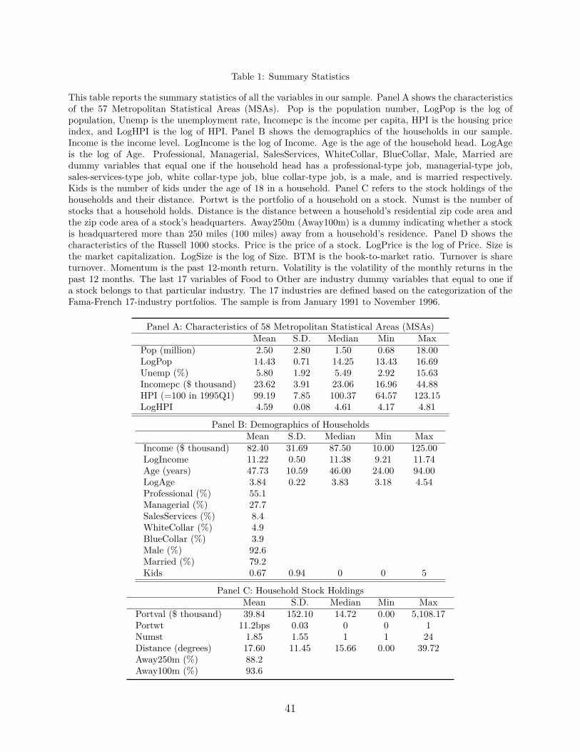
Table 1: Summary Statistics

This table reports the summary statistics of all the variables in our sample. Panel A shows the characteristicsof the 57 Metropolitan Statistical Areas (MSAs). Pop is the population number, LogPop is the log ofpopulation, Unemp is the unemployment rate, Incomepc is the income per capita, HPI is the housing priceindex, and LogHPI is the log of HPI. Panel B shows the demographics of the households in our sample.Income is the income level. LogIncome is the log of Income. Age is the age of the household head. LogAgeis the log of Age. Professional, Managerial, SalesServices, WhiteCollar, BlueCollar, Male, Married aredummy variables that equal one if the household head has a professional-type job, managerial-type job,sales-services-type job, white collar-type job, blue collar-type job, is a male, and is married respectively.Kids is the number of kids under the age of 18 in a household. Panel C refers to the stock holdings of thehouseholds and their distance. Portwt is the portfolio of a household on a stock. Numst is the number ofstocks that a household holds. Distance is the distance between a household’s residential zip code area andthe zip code area of a stock’s headquarters. Away250m (Away100m) is a dummy indicating whether a stockis headquartered more than 250 miles (100 miles) away from a household’s residence. Panel D shows thecharacteristics of the Russell 1000 stocks. Price is the price of a stock. LogPrice is the log of Price. Size isthe market capitalization. LogSize is the log of Size. BTM is the book-to-market ratio. Turnover is shareturnover. Momentum is the past 12-month return. Volatility is the volatility of the monthly returns in thepast 12 months. The last 17 variables of Food to Other are industry dummy variables that equal to one ifa stock belongs to that particular industry. The 17 industries are defined based on the categorization of theFama-French 17-industry portfolios. The sample is from January 1991 to November 1996.

Panel A: Characteristics of 58 Metropolitan Statistical Areas (MSAs)Mean S.D. Median Min Max

Pop (million) 2.50 2.80 1.50 0.68 18.00LogPop 14.43 0.71 14.25 13.43 16.69Unemp (%) 5.80 1.92 5.49 2.92 15.63Incomepc ($ thousand) 23.62 3.91 23.06 16.96 44.88HPI (=100 in 1995Q1) 99.19 7.85 100.37 64.57 123.15LogHPI 4.59 0.08 4.61 4.17 4.81

Panel B: Demographics of HouseholdsMean S.D. Median Min Max

Income ($ thousand) 82.40 31.69 87.50 10.00 125.00LogIncome 11.22 0.50 11.38 9.21 11.74Age (years) 47.73 10.59 46.00 24.00 94.00LogAge 3.84 0.22 3.83 3.18 4.54Professional (%) 55.1Managerial (%) 27.7SalesServices (%) 8.4WhiteCollar (%) 4.9BlueCollar (%) 3.9Male (%) 92.6Married (%) 79.2Kids 0.67 0.94 0 0 5

Panel C: Household Stock HoldingsMean S.D. Median Min Max

Portval ($ thousand) 39.84 152.10 14.72 0.00 5,108.17Portwt 11.2bps 0.03 0 0 1Numst 1.85 1.55 1 1 24Distance (degrees) 17.60 11.45 15.66 0.00 39.72Away250m (%) 88.2Away100m (%) 93.6

41

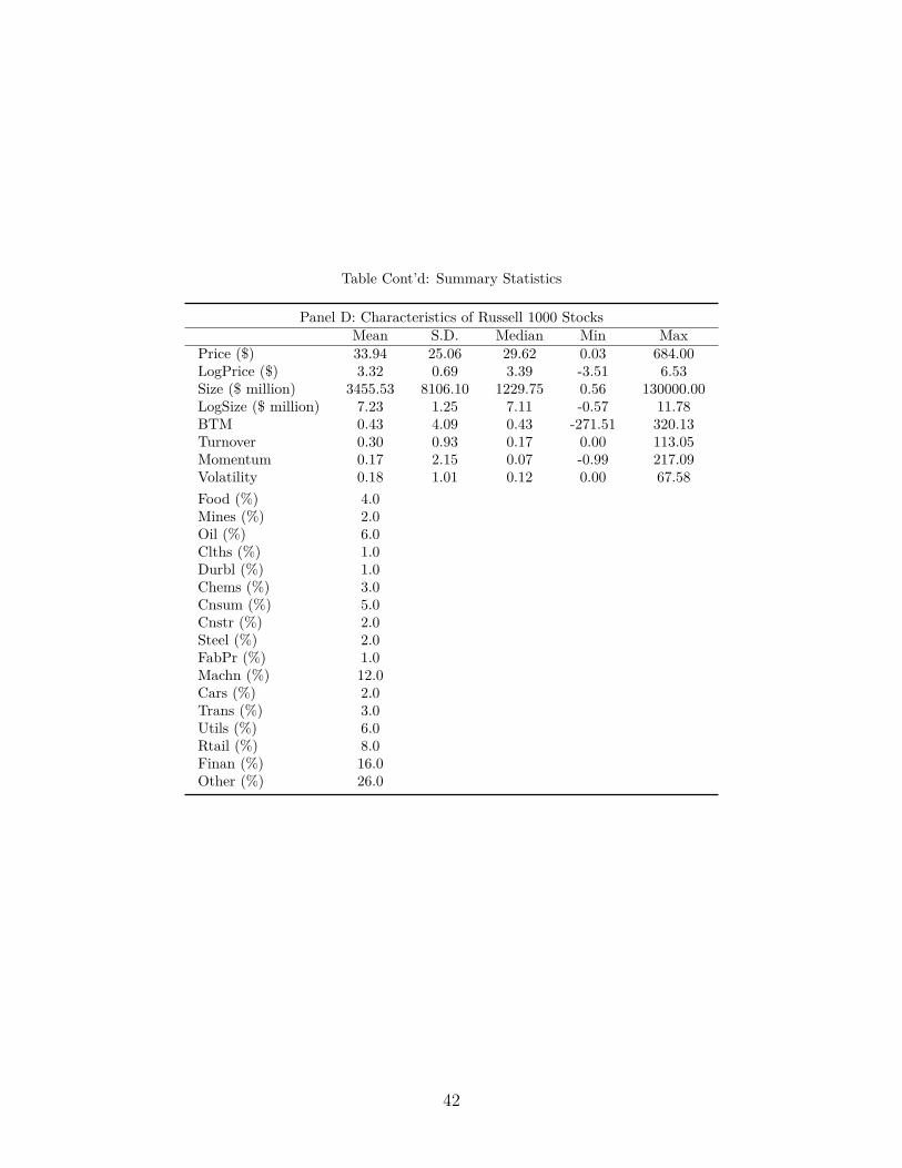
Table Cont’d: Summary Statistics

Panel D: Characteristics of Russell 1000 StocksMean S.D. Median Min Max

Price ($) 33.94 25.06 29.62 0.03 684.00LogPrice ($) 3.32 0.69 3.39 -3.51 6.53Size ($ million) 3455.53 8106.10 1229.75 0.56 130000.00LogSize ($ million) 7.23 1.25 7.11 -0.57 11.78BTM 0.43 4.09 0.43 -271.51 320.13Turnover 0.30 0.93 0.17 0.00 113.05Momentum 0.17 2.15 0.07 -0.99 217.09Volatility 0.18 1.01 0.12 0.00 67.58Food (%) 4.0Mines (%) 2.0Oil (%) 6.0Clths (%) 1.0Durbl (%) 1.0Chems (%) 3.0Cnsum (%) 5.0Cnstr (%) 2.0Steel (%) 2.0FabPr (%) 1.0Machn (%) 12.0Cars (%) 2.0Trans (%) 3.0Utils (%) 6.0Rtail (%) 8.0Finan (%) 16.0Other (%) 26.0

42

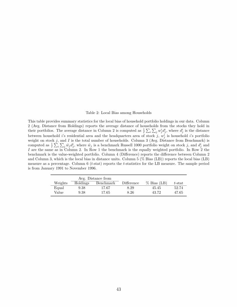
Table 2: Local Bias among Households

This table provides summary statistics for the local bias of household portfolio holdings in our data. Column2 (Avg. Distance from Holdings) reports the average distance of households from the stocks they hold intheir portfolios. The average distance in Column 2 is computed as 1

I

∑i

∑j w

ijd

ij , where di

j is the distancebetween household i’s residential area and the headquarters area of stock j, wi

j is household i’s portfolioweight on stock j, and I is the total number of households. Column 3 (Avg. Distance from Benchmark) iscomputed as 1

I

∑i

∑j w̄jd

ij , where w̄j is a benchmark Russell 1000 portfolio weight on stock j, and di

j andI are the same as in Column 2. In Row 1 the benchmark is the equally weighted portfolio. In Row 2 thebenchmark is the value-weighted portfolio. Column 4 (Difference) reports the difference between Column 2and Column 3, which is the local bias in distance units. Column 5 (% Bias (LB)) reports the local bias (LB)measure as a percentage. Column 6 (t-stat) reports the t-statistics for the LB measure. The sample periodis from January 1991 to November 1996.

Avg. Distance fromWeights Holdings Benchmark Difference % Bias (LB) t-statEqual 9.38 17.67 8.29 45.45 52.74Value 9.38 17.65 8.26 43.72 47.65

43

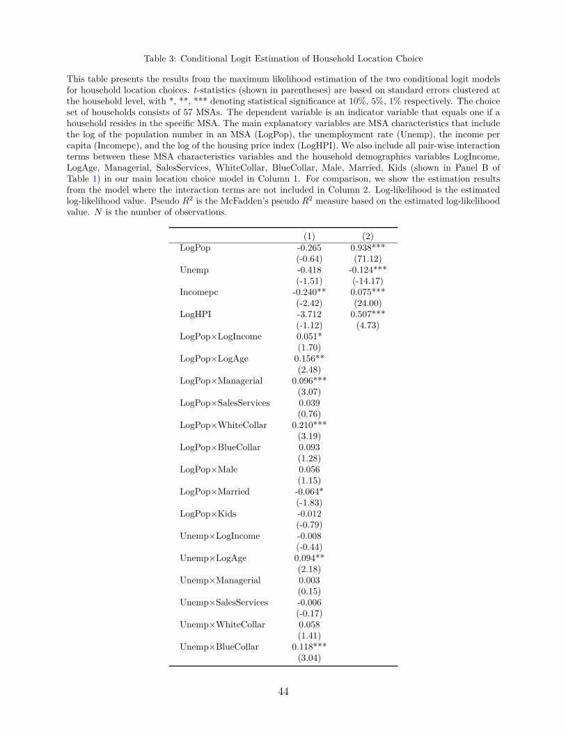
Table 3: Conditional Logit Estimation of Household Location Choice

This table presents the results from the maximum likelihood estimation of the two conditional logit modelsfor household location choices. t-statistics (shown in parentheses) are based on standard errors clustered atthe household level, with *, **, *** denoting statistical significance at 10%, 5%, 1% respectively. The choiceset of households consists of 57 MSAs. The dependent variable is an indicator variable that equals one if ahousehold resides in the specific MSA. The main explanatory variables are MSA characteristics that includethe log of the population number in an MSA (LogPop), the unemployment rate (Unemp), the income percapita (Incomepc), and the log of the housing price index (LogHPI). We also include all pair-wise interactionterms between these MSA characteristics variables and the household demographics variables LogIncome,LogAge, Managerial, SalesServices, WhiteCollar, BlueCollar, Male, Married, Kids (shown in Panel B ofTable 1) in our main location choice model in Column 1. For comparison, we show the estimation resultsfrom the model where the interaction terms are not included in Column 2. Log-likelihood is the estimatedlog-likelihood value. Pseudo R2 is the McFadden’s pseudo R2 measure based on the estimated log-likelihoodvalue. N is the number of observations.

(1) (2)LogPop -0.265 0.938***

(-0.64) (71.12)Unemp -0.418 -0.124***

(-1.51) (-14.17)Incomepc -0.240** 0.075***

(-2.42) (24.00)LogHPI -3.712 0.507***

(-1.12) (4.73)LogPop×LogIncome 0.051*

(1.70)LogPop×LogAge 0.156**

(2.48)LogPop×Managerial 0.096***

(3.07)LogPop×SalesServices 0.039

(0.76)LogPop×WhiteCollar 0.210***

(3.19)LogPop×BlueCollar 0.093

(1.28)LogPop×Male 0.056

(1.15)LogPop×Married -0.064*

(-1.83)LogPop×Kids -0.012

(-0.79)Unemp×LogIncome -0.008

(-0.44)Unemp×LogAge 0.094**

(2.18)Unemp×Managerial 0.003

(0.15)Unemp×SalesServices -0.006

(-0.17)Unemp×WhiteCollar 0.058

(1.41)Unemp×BlueCollar 0.118***

(3.04)

44

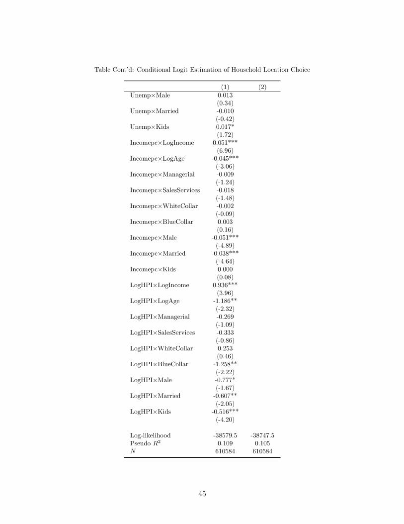
Table Cont’d: Conditional Logit Estimation of Household Location Choice

(1) (2)Unemp×Male 0.013

(0.34)Unemp×Married -0.010

(-0.42)Unemp×Kids 0.017*

(1.72)Incomepc×LogIncome 0.051***

(6.96)Incomepc×LogAge -0.045***

(-3.06)Incomepc×Managerial -0.009

(-1.24)Incomepc×SalesServices -0.018

(-1.48)Incomepc×WhiteCollar -0.002

(-0.09)Incomepc×BlueCollar 0.003

(0.16)Incomepc×Male -0.051***

(-4.89)Incomepc×Married -0.038***

(-4.64)Incomepc×Kids 0.000

(0.08)LogHPI×LogIncome 0.936***

(3.96)LogHPI×LogAge -1.186**

(-2.32)LogHPI×Managerial -0.269

(-1.09)LogHPI×SalesServices -0.333

(-0.86)LogHPI×WhiteCollar 0.253

(0.46)LogHPI×BlueCollar -1.258**

(-2.22)LogHPI×Male -0.777*

(-1.67)LogHPI×Married -0.607**

(-2.05)LogHPI×Kids -0.516***

(-4.20)

Log-likelihood -38579.5 -38747.5Pseudo R2 0.109 0.105N 610584 610584

45

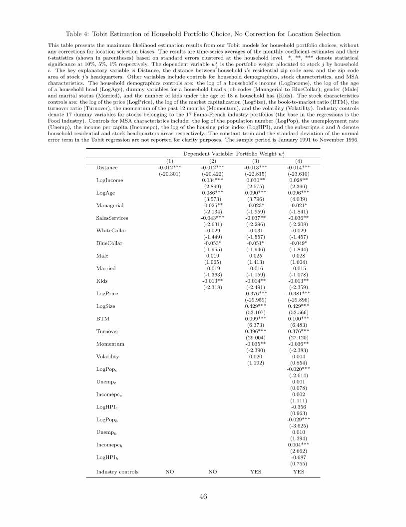
Table 4: Tobit Estimation of Household Portfolio Choice, No Correction for Location SelectionThis table presents the maximum likelihood estimation results from our Tobit models for household portfolio choices, withoutany corrections for location selection biases. The results are time-series averages of the monthly coefficient estimates and theirt-statistics (shown in parentheses) based on standard errors clustered at the household level. *, **, *** denote statisticalsignificance at 10%, 5%, 1% respectively. The dependent variable wi

j is the portfolio weight allocated to stock j by householdi. The key explanatory variable is Distance, the distance between household i’s residential zip code area and the zip codearea of stock j’s headquarters. Other variables include controls for household demographics, stock characteristics, and MSAcharacteristics. The household demographics controls are: the log of a household’s income (LogIncome), the log of the ageof a household head (LogAge), dummy variables for a household head’s job codes (Managerial to BlueCollar), gender (Male)and marital status (Married), and the number of kids under the age of 18 a household has (Kids). The stock characteristicscontrols are: the log of the price (LogPrice), the log of the market capitalization (LogSize), the book-to-market ratio (BTM), theturnover ratio (Turnover), the momentum of the past 12 months (Momentum), and the volatility (Volatility). Industry controlsdenote 17 dummy variables for stocks belonging to the 17 Fama-French industry portfolios (the base in the regressions is theFood industry). Controls for MSA characteristics include: the log of the population number (LogPop), the unemployment rate(Unemp), the income per capita (Incomepc), the log of the housing price index (LogHPI), and the subscripts c and h denotehousehold residential and stock headquarters areas respectively. The constant term and the standard deviation of the normalerror term in the Tobit regression are not reported for clarity purposes. The sample period is January 1991 to November 1996.

Dependent Variable: Portfolio Weight wij

(1) (2) (3) (4)Distance -0.012*** -0.012*** -0.013*** -0.014***

(-20.301) (-20.422) (-22.815) (-23.610)LogIncome 0.034*** 0.030** 0.028**

(2.899) (2.575) (2.396)LogAge 0.086*** 0.090*** 0.096***

(3.573) (3.796) (4.039)Managerial -0.025** -0.023* -0.021*

(-2.134) (-1.959) (-1.841)SalesServices -0.043*** -0.037** -0.036**

(-2.631) (-2.296) (-2.208)WhiteCollar -0.029 -0.031 -0.029

(-1.449) (-1.557) (-1.457)BlueCollar -0.053* -0.051* -0.049*

(-1.955) (-1.946) (-1.844)Male 0.019 0.025 0.028

(1.065) (1.413) (1.604)Married -0.019 -0.016 -0.015

(-1.363) (-1.159) (-1.078)Kids -0.013** -0.014** -0.013**

(-2.318) (-2.491) (-2.359)LogPrice -0.376*** -0.381***

(-29.959) (-29.896)LogSize 0.429*** 0.429***

(53.107) (52.566)BTM 0.099*** 0.100***

(6.373) (6.483)Turnover 0.396*** 0.376***

(29.004) (27.120)Momentum -0.035** -0.036**

(-2.390) (-2.383)Volatility 0.020 0.004

(1.192) (0.854)LogPopc -0.020***

(-2.614)Unempc 0.001

(0.078)Incomepcc 0.002

(1.111)LogHPIc -0.356

(0.963)LogPoph -0.029***

(-3.625)Unemph 0.010

(1.394)Incomepch 0.004***

(2.662)LogHPIh -0.687

(0.755)Industry controls NO NO YES YES

46

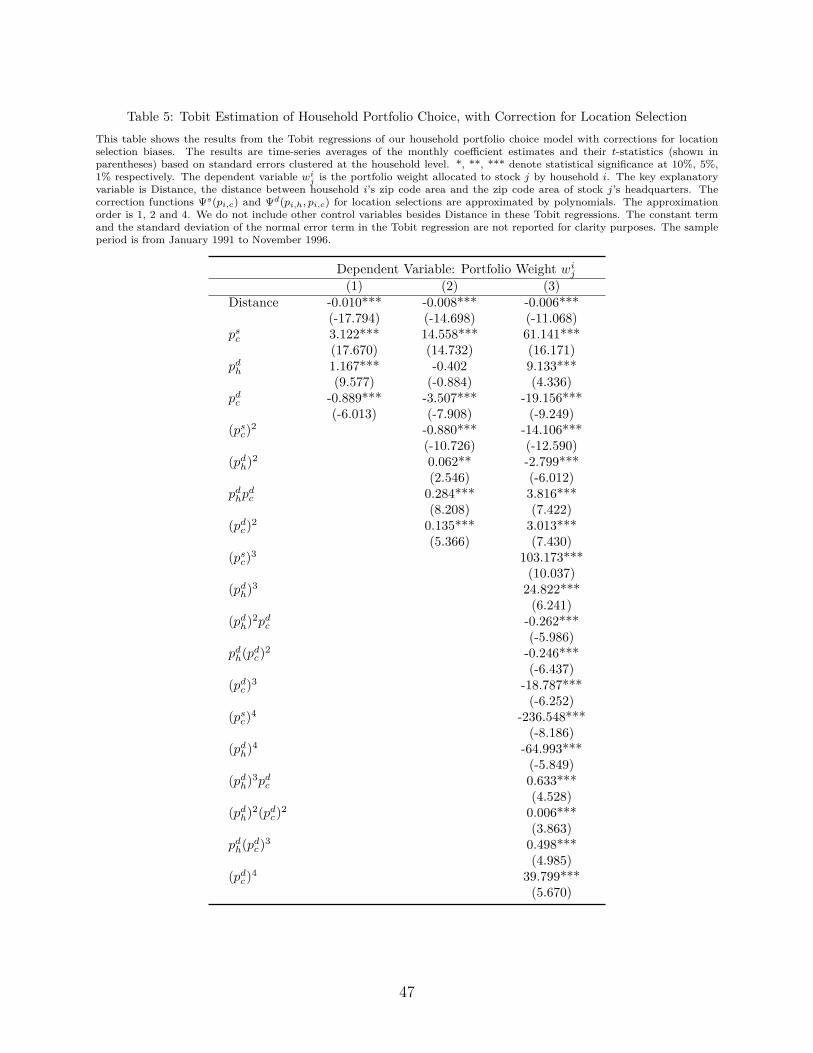
Table 5: Tobit Estimation of Household Portfolio Choice, with Correction for Location SelectionThis table shows the results from the Tobit regressions of our household portfolio choice model with corrections for locationselection biases. The results are time-series averages of the monthly coefficient estimates and their t-statistics (shown inparentheses) based on standard errors clustered at the household level. *, **, *** denote statistical significance at 10%, 5%,1% respectively. The dependent variable wi

j is the portfolio weight allocated to stock j by household i. The key explanatoryvariable is Distance, the distance between household i’s zip code area and the zip code area of stock j’s headquarters. Thecorrection functions Ψs(pi,c) and Ψd(pi,h, pi,c) for location selections are approximated by polynomials. The approximationorder is 1, 2 and 4. We do not include other control variables besides Distance in these Tobit regressions. The constant termand the standard deviation of the normal error term in the Tobit regression are not reported for clarity purposes. The sampleperiod is from January 1991 to November 1996.

Dependent Variable: Portfolio Weight wij

(1) (2) (3)Distance -0.010*** -0.008*** -0.006***

(-17.794) (-14.698) (-11.068)ps

c 3.122*** 14.558*** 61.141***(17.670) (14.732) (16.171)

pdh 1.167*** -0.402 9.133***

(9.577) (-0.884) (4.336)pd

c -0.889*** -3.507*** -19.156***(-6.013) (-7.908) (-9.249)

(psc)2 -0.880*** -14.106***

(-10.726) (-12.590)(pd

h)2 0.062** -2.799***(2.546) (-6.012)

pdhp

dc 0.284*** 3.816***

(8.208) (7.422)(pd

c)2 0.135*** 3.013***(5.366) (7.430)

(psc)3 103.173***

(10.037)(pd

h)3 24.822***(6.241)

(pdh)2pd

c -0.262***(-5.986)

pdh(pd

c)2 -0.246***(-6.437)

(pdc)3 -18.787***

(-6.252)(ps

c)4 -236.548***(-8.186)

(pdh)4 -64.993***

(-5.849)(pd

h)3pdc 0.633***

(4.528)(pd

h)2(pdc)2 0.006***

(3.863)pd

h(pdc)3 0.498***

(4.985)(pd

c)4 39.799***(5.670)

47

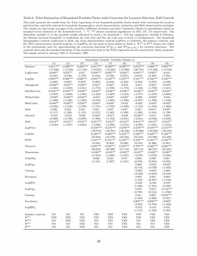
Table 6: Tobit Estimation of Household Portfolio Choice with Correction for Location Selection, Full ControlsThis table presents the results from the Tobit regressions of our household portfolio choice model with corrections for locationselection bias, and with controls for household demographics, stock characteristics, industries and MSA characteristics included.The results are time-series averages of the monthly coefficient estimates and their t-statistics (shown in parentheses) based onstandard errors clustered at the household level. *, **, *** denote statistical significance at 10%, 5%, 1% respectively. Thedependent variable wi

j is the portfolio weight allocated to stock j by household i. The key explanatory variable is Distance,the distance between household i’s residential zip code area and the zip code area of stock j’s headquarters. The householddemographics controls LogIncome to Kids, the stock characteristics controls LogPrice to Volatility, the industry controls, andthe MSA characteristics controls LogPopc to LogHPIh are the same as those shown in Table 4. Ψ1st to Ψ4th denote the ordersof the polynomials used for approximating the correction functions Ψs(pi,c) and Ψd(pi,h, pi,c) for location selections. Theconstant term and the standard deviation of the normal error term in the Tobit regression are not reported for clarity purposes.The sample period is January 1991 to November 1996.

Dependent Variable: Portfolio Weight wij

(1) (2) (3) (4) (5) (6) (7) (8) (9)Distance -0.011*** -0.008*** -0.006*** -0.011*** -0.009*** -0.007*** -0.012*** -0.009*** -0.007***

(-17.890) (-14.769) (-11.140) (-19.944) (-16.682) (-13.280) (-20.716) (-17.356) (-13.726)LogIncome 0.029** 0.027** 0.017 0.039*** 0.032*** 0.024** 0.043*** 0.030** 0.019

(2.445) (2.196) (1.379) (3.343) (2.739) (2.047) (3.637) (2.497) (1.591)LogAge 0.083*** 0.089*** 0.088*** 0.094*** 0.100*** 0.105*** 0.101*** 0.102*** 0.105***

(3.468) (3.687) (3.657) (3.995) (4.216) (4.435) (4.294) (4.319) (4.426)Managerial -0.029** -0.027** -0.029** -0.021* -0.021* -0.019 -0.017 -0.021* -0.019*

(-2.401) (-2.303) (-2.451) (-1.774) (-1.769) (-1.575) (-1.434) (-1.759) (-1.651)SalesServices -0.044*** -0.043*** -0.040** -0.039** -0.038** -0.036** -0.038** -0.037** -0.034**

(-2.697) (-2.669) (-2.494) (-2.432) (-2.365) (-2.218) (-2.377) (-2.285) (-2.092)WhiteCollar -0.038* -0.048** -0.042** -0.018 -0.035* -0.034* -0.008 -0.040* -0.034

(-1.866) (-2.286) (-1.989) (-0.910) (-1.692) (-1.646) (-0.387) (-1.896) (-1.640)BlueCollar -0.056** -0.058** -0.053** -0.045* -0.049* -0.043 -0.039 -0.048* -0.043*

(-2.092) (-2.132) (-1.970) (-1.731) (-1.859) (-1.630) (-1.473) (-1.835) (-1.663)Male 0.020 0.024 0.021 0.021 0.027 0.027 0.021 0.031* 0.030*

(1.117) (1.356) (1.155) (1.215) (1.582) (1.590) (1.236) (1.819) (1.720)Married -0.013 -0.010 -0.001 -0.023* -0.015 -0.008 -0.028** -0.011 -0.004

(-0.968) (-0.740) (-0.095) (-1.680) (-1.104) (-0.631) (-2.041) (-0.840) (-0.350)Kids -0.013** -0.012** -0.012** -0.015*** -0.013** -0.013** -0.014*** -0.012** -0.012**

(-2.244) (-2.047) (-2.064) (-2.626) (-2.390) (-2.313) (-2.597) (-2.261) (-2.212)LogPrice -0.376*** -0.375*** -0.370*** -0.379*** -0.378*** -0.374***

(-29.875) (-29.701) (-29.438) (-29.690) (-29.620) (-29.423)LogSize 0.430*** 0.428*** 0.423*** 0.429*** 0.428*** 0.426***

(52.684) (52.579) (52.524) (52.525) (52.389) (52.429)BTM 0.101*** 0.101*** 0.102*** 0.102*** 0.101*** 0.102***

(6.442) (6.402) (6.390) (6.534) (6.466) (6.461)Turnover 0.391*** 0.385*** 0.370*** 0.370*** 0.368*** 0.356***

(28.643) (28.299) (27.110) (26.714) (26.527) (25.424)Momentum -0.036** -0.035** -0.035** -0.037** -0.036** -0.036**

(-2.419) (-2.409) (-2.407) (-2.427) (-2.372) (-2.384)Volatility 0.020 0.024 0.017 0.003 0.006 0.001

(1.181) (1.307) (1.231) (0.870) (0.933) (0.870)LogPopc 0.008 -0.013 -0.040*

(0.718) (-0.790) (-1.832)Unempc -0.002 -0.003 -0.003

(-0.440) (-0.684) (-0.544)Incomepcc 0.003 0.001 -0.004

(1.542) (0.267) (-1.542)LogHPIc -0.303 -0.199 -0.047

(1.326) (1.213) (0.839)LogPoph 0.010 0.013 -0.110***

(0.798) (0.514) (-4.760)Unemph 0.011 0.007 0.023***

(1.452) (1.000) (3.331)Incomepch 0.007*** 0.006*** -0.005*

(3.919) (2.784) (-1.892)LogHPIh -0.552 -0.441 0.016

(1.113) (1.349) (1.385)Industry controls NO NO NO YES YES YES YES YES YESΨ1st YES YES YES YES YES YES YES YES YESΨ2nd NO YES YES NO YES YES NO YES YESΨ3rd NO NO YES NO NO YES NO NO YESΨ4th NO NO YES NO NO YES NO NO YES

48

Table 7: Economic Effects of Distance on Household Portfolio Weights

This table shows the economic effect of a one standard deviation increase in Distance on the portfolioweight of a household on a stock, from different specifications of our household portfolio choice model. Theeconomic effect is calculated based on the marginal effect of Distance on the portfolio weight from the Tobitestimation, with all other control variables anchored at their mean levels. The marginal effect is computedin each monthly estimation and then averaged across all months. Corrections denote whether the 4th ordercorrection function for location selection bias is included, and Full Controls denote whether the full set ofcontrols for household demographics, stock characteristics, industry and MSA characteristics are included.The sample period is January 1991 to November 1996.

Full Controls No YesCorrectionsNo -3.8bps -1.9bpsYes -1.8bps -0.9bps

49

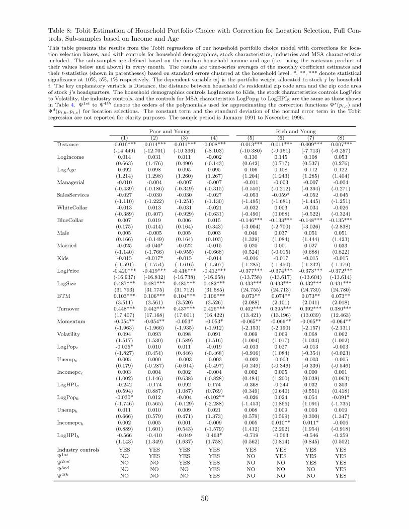
Table 8: Tobit Estimation of Household Portfolio Choice with Correction for Location Selection, Full Con-trols, Sub-samples based on Income and AgeThis table presents the results from the Tobit regressions of our household portfolio choice model with corrections for loca-tion selection biases, and with controls for household demographics, stock characteristics, industries and MSA characteristicsincluded. The sub-samples are defined based on the median household income and age (i.e. using the cartesian product oftheir values below and above) in every month. The results are time-series averages of the monthly coefficient estimates andtheir t-statistics (shown in parentheses) based on standard errors clustered at the household level. *, **, *** denote statisticalsignificance at 10%, 5%, 1% respectively. The dependent variable wi

j is the portfolio weight allocated to stock j by householdi. The key explanatory variable is Distance, the distance between household i’s residential zip code area and the zip code areaof stock j’s headquarters. The household demographics controls LogIncome to Kids, the stock characteristics controls LogPriceto Volatility, the industry controls, and the controls for MSA characteristics LogPopH to LogHPIS are the same as those shownin Table 4. Ψ1st to Ψ4th denote the orders of the polynomials used for approximating the correction functions Ψs(pi,c) andΨd(pi,h, pi,c) for location selections. The constant term and the standard deviation of the normal error term in the Tobitregression are not reported for clarity purposes. The sample period is January 1991 to November 1996.

Poor and Young Rich and Young(1) (2) (3) (4) (5) (6) (7) (8)

Distance -0.016*** -0.014*** -0.011*** -0.008*** -0.013*** -0.011*** -0.009*** -0.007***(-14.449) (-12.701) (-10.336) (-8.103) (-10.380) (-9.161) (-7.713) (-6.257)

LogIncome 0.014 0.031 0.011 -0.002 0.130 0.145 0.108 0.053(0.663) (1.476) (0.490) (-0.143) (0.642) (0.717) (0.537) (0.276)

LogAge 0.092 0.098 0.095 0.095 0.106 0.108 0.112 0.122(1.214) (1.298) (1.260) (1.267) (1.204) (1.243) (1.285) (1.404)

Managerial -0.010 -0.004 -0.007 -0.007 -0.011 -0.003 -0.007 -0.004(-0.439) (-0.186) (-0.349) (-0.315) (-0.550) (-0.212) (-0.394) (-0.271)

SalesServices -0.027 -0.030 -0.030 -0.027 -0.053 -0.059* -0.052 -0.045(-1.110) (-1.222) (-1.251) (-1.130) (-1.495) (-1.681) (-1.445) (-1.251)

WhiteCollar -0.013 0.013 -0.031 -0.021 -0.032 0.003 -0.034 -0.026(-0.389) (0.407) (-0.929) (-0.631) (-0.490) (0.068) (-0.522) (-0.324)

BlueCollar 0.007 0.019 0.006 0.015 -0.146*** -0.133*** -0.148*** -0.135***(0.175) (0.414) (0.164) (0.343) (-3.004) (-2.700) (-3.026) (-2.838)

Male 0.005 -0.005 0.005 0.003 0.046 0.037 0.051 0.051(0.166) (-0.149) (0.164) (0.103) (1.339) (1.084) (1.444) (1.423)

Married -0.025 -0.040* -0.022 -0.015 0.020 0.001 0.027 0.033(-1.140) (-1.766) (-0.955) (-0.668) (0.524) (-0.015) (0.688) (0.822)

Kids -0.015 -0.017* -0.015 -0.014 -0.016 -0.017 -0.015 -0.015(-1.591) (-1.754) (-1.616) (-1.507) (-1.285) (-1.450) (-1.242) (-1.179)

LogPrice -0.420*** -0.419*** -0.416*** -0.412*** -0.377*** -0.374*** -0.373*** -0.372***(-16.937) (-16.832) (-16.738) (-16.658) (-13.758) (-13.617) (-13.604) (-13.614)

LogSize 0.487*** 0.487*** 0.485*** 0.482*** 0.433*** 0.433*** 0.432*** 0.431***(31.793) (31.775) (31.712) (31.685) (24.755) (24.713) (24.730) (24.780)

BTM 0.103*** 0.106*** 0.104*** 0.106*** 0.073** 0.074** 0.073** 0.073**(3.511) (3.561) (3.520) (3.526) (2.088) (2.101) (2.041) (2.018)

Turnover 0.448*** 0.442*** 0.437*** 0.426*** 0.402*** 0.395*** 0.392*** 0.380***(17.407) (17.168) (17.001) (16.422) (13.421) (13.196) (13.039) (12.463)

Momentum -0.054** -0.054** -0.053* -0.053* -0.065** -0.066** -0.065** -0.064**(-1.963) (-1.966) (-1.935) (-1.912) (-2.153) (-2.190) (-2.157) (-2.131)

Volatility 0.094 0.093 0.098 0.091 0.069 0.069 0.068 0.062(1.517) (1.530) (1.589) (1.516) (1.004) (1.017) (1.034) (1.002)

LogPopc -0.025* 0.010 0.011 -0.019 -0.013 0.027 -0.013 -0.003(-1.827) (0.454) (0.446) (-0.468) (-0.916) (1.084) (-0.354) (-0.023)

Unempc 0.005 0.000 -0.003 -0.003 -0.002 -0.003 -0.003 -0.005(0.179) (-0.287) (-0.614) (-0.497) (-0.249) (-0.346) (-0.339) (-0.546)

Incomepcc 0.003 0.004 0.002 -0.004 0.002 0.005 0.000 0.001(1.002) (1.146) (0.638) (-0.828) (0.484) (1.200) (0.038) (0.063)

LogHPIc -0.242 -0.174 0.092 0.174 -0.368 -0.244 0.032 0.303(0.594) (0.887) (1.087) (0.769) (0.349) (0.640) (0.551) (0.418)

LogPoph -0.030* 0.012 -0.004 -0.102** -0.026 0.024 0.054 -0.091*(-1.746) (0.565) (-0.129) (-2.288) (-1.453) (0.866) (1.091) (-1.735)

Unemph 0.011 0.010 0.009 0.021 0.008 0.009 0.003 0.019(0.666) (0.579) (0.471) (1.373) (0.579) (0.599) (0.300) (1.347)

Incomepch 0.002 0.005 0.001 -0.009 0.005 0.010** 0.011* -0.006(0.889) (1.601) (0.543) (-1.579) (1.412) (2.292) (1.954) (-0.918)

LogHPIh -0.566 -0.410 -0.049 0.463* -0.719 -0.563 -0.546 -0.259(1.143) (1.349) (1.637) (1.758) (0.562) (0.814) (0.845) (0.502)

Industry controls YES YES YES YES YES YES YES YESΨ1st NO YES YES YES NO YES YES YESΨ2nd NO NO YES YES NO NO YES YESΨ3rd NO NO NO YES NO NO NO YESΨ4th NO NO NO YES NO NO NO YES

50

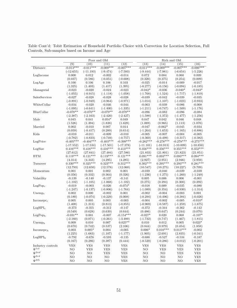
Table Cont’d: Tobit Estimation of Household Portfolio Choice with Correction for Location Selection, FullControls, Sub-samples based on Income and Age

Poor and Old Rich and Old(9) (10) (11) (12) (13) (14) (15) (16)

Distance -0.013*** -0.011*** -0.009*** -0.007*** -0.011*** -0.009*** -0.007*** -0.006***(-12.655) (-11.193) (-9.474) (-7.593) (-9.444) (-7.981) (-6.654) (-5.226)

LogIncome 0.000 0.012 -0.002 -0.014 0.072 0.084 0.060 0.009(0.037) (0.586) (-0.051) (-0.608) (0.320) (0.375) (0.254) (0.009)

LogAge 0.100 0.106 0.106 0.103 -0.025 -0.014 -0.009 -0.017(1.325) (1.403) (1.417) (1.395) (-0.277) (-0.156) (-0.094) (-0.185)

Managerial -0.023 -0.020 -0.024 -0.023 -0.042* -0.036 -0.040* -0.043*(-1.055) (-0.915) (-1.118) (-1.058) (-1.768) (-1.524) (-1.717) (-1.819)

SalesServices -0.027 -0.028 -0.028 -0.028 -0.039 -0.042 -0.039 -0.035(-0.891) (-0.949) (-0.964) (-0.971) (-1.014) (-1.107) (-1.023) (-0.933)

WhiteCollar -0.034 -0.020 -0.046 -0.044 -0.063 -0.039 -0.086 -0.068(-1.095) (-0.641) (-1.400) (-1.335) (-1.211) (-0.747) (-1.509) (-1.176)

BlueCollar -0.078** -0.070** -0.079** -0.078** -0.096 -0.082 -0.096 -0.084(-2.387) (-2.163) (-2.420) (-2.427) (-1.588) (-1.372) (-1.477) (-1.256)

Male 0.045 0.041 0.054* 0.049 0.047 0.042 0.046 0.048(1.526) (1.394) (1.826) (1.628) (1.069) (0.965) (1.113) (1.076)

Married 0.002 -0.010 0.007 0.014 -0.047 -0.062* -0.045 -0.034(0.059) (-0.417) (0.289) (0.614) (-1.264) (-1.653) (-1.165) (-0.886)

Kids -0.010 -0.011 -0.009 -0.010 -0.005 -0.007 -0.004 -0.005(-0.782) (-0.833) (-0.749) (-0.757) (-0.360) (-0.499) (-0.317) (-0.382)

LogPrice -0.405*** -0.404*** -0.403*** -0.399*** -0.282*** -0.278*** -0.278*** -0.275***(-17.552) (-17.534) (-17.501) (-17.378) (-11.101) (-10.913) (-10.899) (-10.850)

LogSize 0.416*** 0.416*** 0.416*** 0.413*** 0.356*** 0.356*** 0.355*** 0.352***(27.612) (27.641) (27.484) (27.586) (21.833) (21.801) (21.823) (21.851)

BTM 0.119*** 0.121*** 0.119*** 0.121*** 0.091*** 0.093*** 0.093*** 0.094***(4.314) (4.343) (4.295) (4.285) (2.927) (2.951) (2.946) (2.959)

Turnover 0.330*** 0.325*** 0.323*** 0.312*** 0.302*** 0.295*** 0.293*** 0.281***(12.793) (12.650) (12.578) (12.060) (10.547) (10.275) (10.227) (9.709)

Momentum 0.001 0.001 0.002 0.001 -0.039 -0.040 -0.039 -0.039(0.356) (0.332) (0.364) (0.326) (-1.236) (-1.275) (-1.260) (-1.249)

Volatility -0.139 -0.140 -0.137 -0.141 0.005 0.006 0.006 -0.001(-1.102) (-1.105) (-1.068) (-1.102) (0.275) (0.294) (0.300) (0.292)

LogPopc -0.019 -0.003 -0.026 -0.074* -0.018 0.009 -0.035 -0.080(-1.247) (-0.137) (-0.806) (-1.764) (-1.089) (0.354) (-0.930) (-1.314)

Unempc 0.002 0.000 -0.002 0.001 -0.002 -0.004 -0.003 0.001(0.180) (-0.074) (-0.229) (0.068) (-0.294) (-0.496) (-0.384) (-0.026)

Incomepcc 0.005 0.005 0.003 -0.003 -0.004 -0.002 -0.005 -0.010*(1.408) (1.313) (0.813) (-0.855) (-0.969) (-0.587) (-1.259) (-1.675)

LogHPIc -0.373 -0.355 -0.312 -0.147 -0.372 -0.344 -0.362 -0.142(0.549) (0.628) (0.630) (0.644) (0.486) (0.647) (0.244) (0.070)

LogPoph -0.031** 0.001 -0.007 -0.154*** -0.027* 0.020 0.068 -0.107*(-2.160) (0.071) (-0.261) (-3.489) (-1.732) (0.747) (1.467) (-1.815)

Unemph 0.009 0.010 0.007 0.025** 0.010 0.012 0.005 0.023*(0.670) (0.742) (0.537) (2.106) (0.844) (0.979) (0.454) (1.858)

Incomepch 0.003 0.005* 0.004 -0.005 0.006* 0.010*** 0.013*** -0.002(1.225) (1.683) (1.107) (-1.177) (1.905) (2.691) (2.835) (-0.341)

LogHPIh -0.792 -0.676 -0.593 -0.135 -0.688 -0.527 -0.534 -0.187(0.167) (0.286) (0.387) (0.444) (-0.520) (-0.286) (-0.012) (-0.201)

Industry controls YES YES YES YES YES YES YES YESΨ1st NO YES YES YES NO YES YES YESΨ2nd NO NO YES YES NO NO YES YESΨ3rd NO NO NO YES NO NO NO YESΨ4th NO NO NO YES NO NO NO YES

51

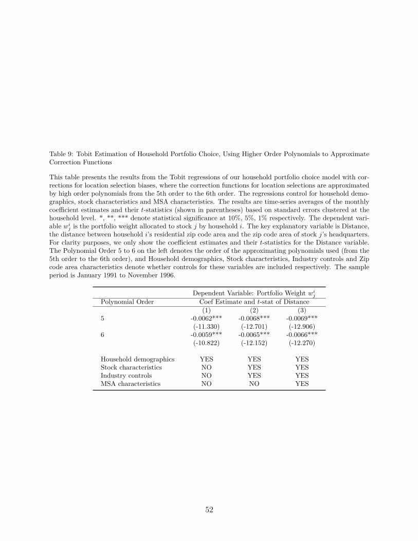
Table 9: Tobit Estimation of Household Portfolio Choice, Using Higher Order Polynomials to ApproximateCorrection Functions

This table presents the results from the Tobit regressions of our household portfolio choice model with cor-rections for location selection biases, where the correction functions for location selections are approximatedby high order polynomials from the 5th order to the 6th order. The regressions control for household demo-graphics, stock characteristics and MSA characteristics. The results are time-series averages of the monthlycoefficient estimates and their t-statistics (shown in parentheses) based on standard errors clustered at thehousehold level. *, **, *** denote statistical significance at 10%, 5%, 1% respectively. The dependent vari-able wi

j is the portfolio weight allocated to stock j by household i. The key explanatory variable is Distance,the distance between household i’s residential zip code area and the zip code area of stock j’s headquarters.For clarity purposes, we only show the coefficient estimates and their t-statistics for the Distance variable.The Polynomial Order 5 to 6 on the left denotes the order of the approximating polynomials used (from the5th order to the 6th order), and Household demographics, Stock characteristics, Industry controls and Zipcode area characteristics denote whether controls for these variables are included respectively. The sampleperiod is January 1991 to November 1996.

Dependent Variable: Portfolio Weight wij

Polynomial Order Coef Estimate and t-stat of Distance(1) (2) (3)

5 -0.0062*** -0.0068*** -0.0069***(-11.330) (-12.701) (-12.906)

6 -0.0059*** -0.0065*** -0.0066***(-10.822) (-12.152) (-12.270)

Household demographics YES YES YESStock characteristics NO YES YESIndustry controls NO YES YESMSA characteristics NO NO YES

52

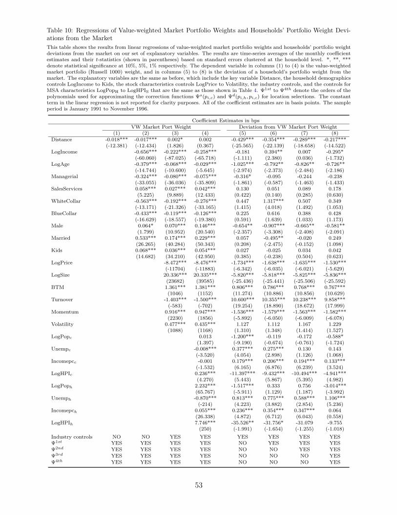
Table 10: Regressions of Value-weighted Market Portfolio Weights and Households’ Portfolio Weight Devi-ations from the MarketThis table shows the results from linear regressions of value-weighted market portfolio weights and households’ portfolio weightdeviations from the market on our set of explanatory variables. The results are time-series averages of the monthly coefficientestimates and their t-statistics (shown in parentheses) based on standard errors clustered at the household level. *, **, ***denote statistical significance at 10%, 5%, 1% respectively. The dependent variable in columns (1) to (4) is the value-weightedmarket portfolio (Russell 1000) weight, and in columns (5) to (8) is the deviation of a household’s portfolio weight from themarket. The explanatory variables are the same as before, which include the key variable Distance, the household demographicscontrols LogIncome to Kids, the stock characteristics controls LogPrice to Volatility, the industry controls, and the controls forMSA characteristics LogPopH to LogHPIS that are the same as those shown in Table 4. Ψ1st to Ψ4th denote the orders of thepolynomials used for approximating the correction functions Ψs(pi,c) and Ψd(pi,h, pi,c) for location selections. The constantterm in the linear regression is not reported for clarity purposes. All of the coefficient estimates are in basis points. The sampleperiod is January 1991 to November 1996.

Coefficient Estimates in bpsVW Market Port Weight Deviation from VW Market Port Weight

(1) (2) (3) (4) (5) (6) (7) (8)Distance -0.018*** -0.017*** 0.002* 0.002 -0.429*** -0.354*** -0.289*** -0.217***

(-12.381) (-12.434) (1.826) (0.367) (-25.565) (-22.139) (-18.658) (-14.522)LogIncome -0.656*** -0.222*** -0.258*** -0.181 0.394** 0.007 -0.295*

(-60.060) (-87.025) (-65.718) (-1.111) (2.380) (0.036) (-1.732)LogAge -0.379*** -0.068*** -0.029*** -1.025*** -0.792** -0.826** -0.726**

(-14.744) (-10.600) (-5.645) (-2.974) (-2.373) (-2.484) (-2.186)Managerial -0.324*** -0.080*** -0.075*** -0.316* -0.095 -0.244 -0.238

(-33.055) (-36.036) (-35.809) (-1.861) (-0.587) (-1.463) (-1.433)SalesServices 0.058*** 0.027*** 0.042*** 0.130 0.051 0.089 0.178

(5.225) (9.889) (12.433) (0.422) (0.140) (0.285) (0.630)WhiteCollar -0.563*** -0.192*** -0.276*** 0.447 1.317*** 0.507 0.349

(-13.171) (-21.326) (-33.165) (1.415) (4.018) (1.492) (1.053)BlueCollar -0.433*** -0.119*** -0.126*** 0.225 0.616 0.388 0.428

(-16.629) (-18.557) (-19.380) (0.591) (1.639) (1.033) (1.173)Male 0.064* 0.070*** 0.146*** -0.654** -0.907*** -0.665** -0.581**

(1.799) (10.952) (20.540) (-2.357) (-3.308) (-2.408) (-2.091)Married 0.533*** 0.174*** 0.229*** 0.057 -0.495** -0.020 0.249

(26.265) (40.284) (50.343) (0.208) (-2.475) (-0.152) (1.098)Kids 0.068*** 0.036*** 0.054*** 0.027 -0.025 0.034 0.042

(14.682) (34.210) (42.950) (0.385) (-0.238) (0.504) (0.623)LogPrice -8.472*** -8.476*** -1.734*** -1.638*** -1.635*** -1.530***

(-11704) (-11883) (-6.342) (-6.035) (-6.021) (-5.629)LogSize 20.336*** 20.335*** -5.820*** -5.818*** -5.825*** -5.836***

(23682) (39585) (-25.436) (-25.441) (-25.506) (-25.592)BTM 1.361*** 1.381*** 0.806*** 0.786*** 0.768*** 0.767***

(1046) (1152) (11.274) (10.886) (10.856) (10.629)Turnover -1.403*** -1.500*** 10.600*** 10.355*** 10.238*** 9.858***

(-583) (-702) (19.254) (18.890) (18.672) (17.999)Momentum 0.916*** 0.947*** -1.536*** -1.579*** -1.563*** -1.582***

(2230) (1856) (-5.892) (-6.050) (-6.009) (-6.078)Volatility 0.477*** 0.435*** 1.127 1.112 1.167 1.229

(1088) (1168) (1.310) (1.348) (1.414) (1.527)LogPopc 0.013 -1.200*** -0.119 -0.172 -0.588*

(1.397) (-9.190) (-0.674) (-0.761) (-1.724)Unempc -0.008*** 0.377*** 0.275*** 0.130 0.143

(-3.520) (4.054) (2.898) (1.126) (1.068)Incomepcc -0.001 0.179*** 0.206*** 0.194*** 0.133***

(-1.532) (6.165) (6.876) (6.239) (3.524)LogHPIc 0.236*** -11.397*** -9.432*** -10.494*** -4.941***

(4.270) (5.443) (5.867) (5.395) (4.982)LogPoph 2.232*** -1.517*** 0.333 0.756 -3.014***

(65.767) (-5.911) (1.129) (1.187) (-3.992)Unemph -0.870*** 0.813*** 0.775*** 0.588*** 1.106***

(-214) (4.223) (3.882) (2.854) (5.236)Incomepch 0.055*** 0.236*** 0.354*** 0.347*** 0.064

(26.338) (4.872) (6.712) (6.043) (0.558)LogHPIh 7.746*** -35.526** -31.756* -31.079 -9.755

(250) (-1.991) (-1.654) (-1.255) (-1.018)Industry controls NO NO YES YES YES YES YES YESΨ1st YES YES YES YES NO YES YES YESΨ2nd YES YES YES YES NO NO YES YESΨ3rd YES YES YES YES NO NO NO YESΨ4th YES YES YES YES NO NO NO YES

53

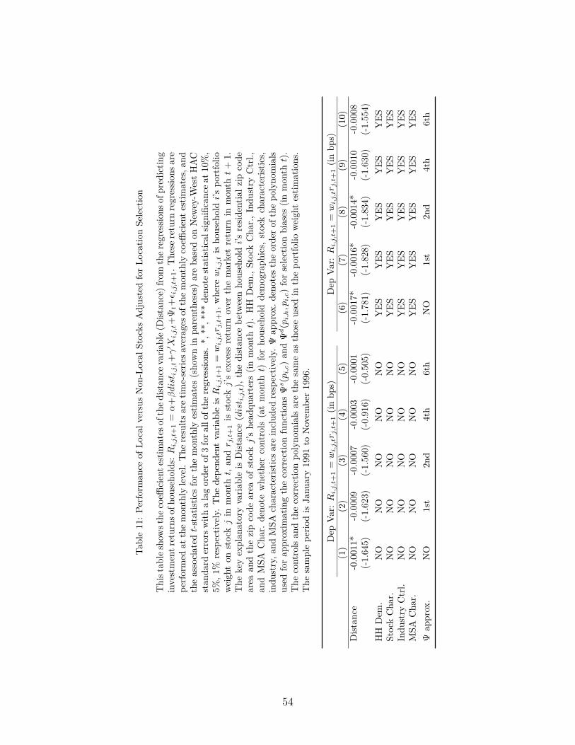
Table11:Pe

rforman

ceof

Localv

ersusNon

-Local

Stocks

AdjustedforLo

catio

nSe

lection

Thist

ableshow

sthe

coeffi

ciente

stim

ates

ofthed

istan

cevaria

ble(

Dist

ance)from

ther

egressions

ofpredictin

ginvestmentr

eturns

ofho

useh

olds:R

i,j,

t+1

=α

+βdist i

,j,t

+γ′ X

i,j,

t+

Ψt+ε i

,j,t

+1.

The

sereturn

regressio

nsare

performed

atthemon

thly

level.The

results

aretim

e-serie

saverageso

fthe

mon

thly

coeffi

ciente

stim

ates,a

ndtheassociated

t-statist

icsforthemon

thly

estim

ates

(sho

wnin

parenthe

ses)

areba

sedon

New

ey-W

estHAC

stan

dard

errors

with

alagorde

rof3

fora

llof

theregressio

ns.*,

**,*

**de

note

statist

ical

signific

ance

at10%,

5%,1

%respectiv

ely.

The

depe

ndentvaria

bleisR

i,j,

t+1

=w

i,j,

tr j

,t+

1,whe

rew

i,j,

tis

househ

oldi’s

portfolio

weigh

ton

stockjin

mon

tht,

andr j

,t+

1is

stockj’sexcess

return

over

themarketreturn

inmon

tht

+1.

The

keyexplan

atoryvaria

bleis

Dist

ance

(dist i

,j,t),

thedistan

cebe

tweenho

useholdi’s

resid

entia

lzip

code

area

andthezipcode

area

ofstockj’she

adqu

arters

(inmon

tht).HH

Dem

.,StockCha

r.,Indu

stry

Ctrl.,

andMSA

Cha

r.deno

tewhe

ther

controls

(atmon

tht)

forho

useh

oldde

mograph

ics,

stockcharacteris

tics,

indu

stry,a

ndMSA

characteris

ticsareinclud

edrespectiv

ely.

Ψap

prox.d

enotes

theorde

rof

thepo

lyno

mials

used

forap

proxim

atingthecorrectio

nfunc

tions

Ψs(p

i,c)an

dΨ

d(p

i,h,p

i,c)forselectionbiases

(inmon

tht).

The

controlsan

dthecorrectio

npo

lyno

mialsarethesameas

thoseused

inthepo

rtfolio

weigh

testim

ations.

The

samplepe

riodis

Janu

ary1991

toNovem

ber1996.

Dep

Var:R

i,j,

t+1

=w

i,j,

tr j

,t+

1(in

bps)

Dep

Var:R

i,j,

t+1

=w

i,j,

tr j

,t+

1(in

bps)

(1)

(2)

(3)

(4)

(5)

(6)

(7)

(8)

(9)

(10)

Dist

ance

-0.0011*

-0.0009

-0.0007

-0.0003

-0.0001

-0.0017*

-0.0016*

-0.0014*

-0.0010

-0.0008

(-1.645)

(-1.623)

(-1.560)

(-0.916)

(-0.505)

(-1.781)

(-1.828)

(-1.834)

(-1.630)

(-1.554)

HH

Dem

.NO

NO

NO

NO

NO

YES

YES

YES

YES

YES

StockCha

r.NO

NO

NO

NO

NO

YES

YES

YES

YES

YES

Indu

stry

Ctrl.

NO

NO

NO

NO

NO

YES

YES

YES

YES

YES

MSA

Cha

r.NO

NO

NO

NO

NO

YES

YES

YES

YES

YES

Ψap

prox.

NO

1st

2nd

4th

6th

NO

1st

2nd

4th

6th

54

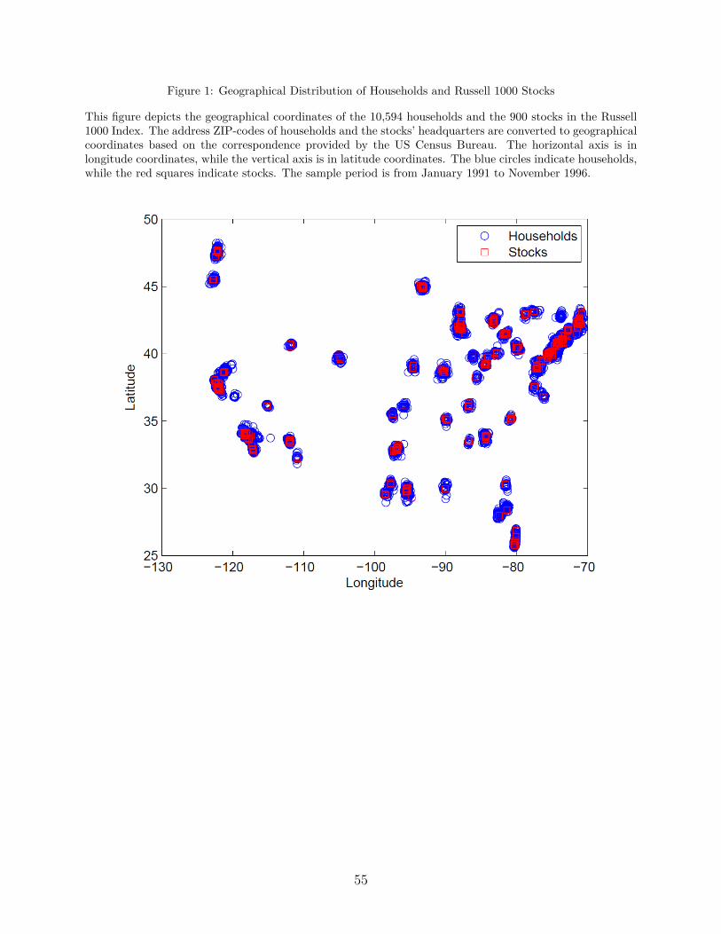
Figure 1: Geographical Distribution of Households and Russell 1000 Stocks

This figure depicts the geographical coordinates of the 10,594 households and the 900 stocks in the Russell1000 Index. The address ZIP-codes of households and the stocks’ headquarters are converted to geographicalcoordinates based on the correspondence provided by the US Census Bureau. The horizontal axis is inlongitude coordinates, while the vertical axis is in latitude coordinates. The blue circles indicate households,while the red squares indicate stocks. The sample period is from January 1991 to November 1996.

55

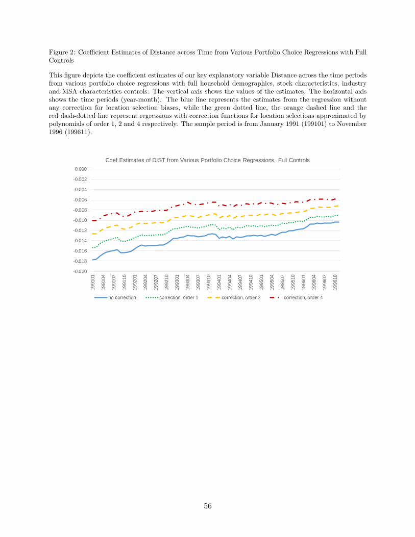
Figure 2: Coefficient Estimates of Distance across Time from Various Portfolio Choice Regressions with FullControls

This figure depicts the coefficient estimates of our key explanatory variable Distance across the time periodsfrom various portfolio choice regressions with full household demographics, stock characteristics, industryand MSA characteristics controls. The vertical axis shows the values of the estimates. The horizontal axisshows the time periods (year-month). The blue line represents the estimates from the regression withoutany correction for location selection biases, while the green dotted line, the orange dashed line and thered dash-dotted line represent regressions with correction functions for location selections approximated bypolynomials of order 1, 2 and 4 respectively. The sample period is from January 1991 (199101) to November1996 (199611).

-0.020

-0.018

-0.016

-0.014

-0.012

-0.010

-0.008

-0.006

-0.004

-0.002

0.000

19

9101

19

9104

19

9107

19

9110

19

9201

19

9204

19

9207

19

9210

19

9301

19

9304

19

9307

19

9310

19

9401

19

9404

19

9407

19

9410

19

9501

19

9504

19

9507

19

9510

19

9601

19

9604

19

9607

19

9610

Coef Estimates of DIST from Various Portfolio Choice Regressions, Full Controls

no correction correction, order 1 correction, order 2 correction, order 4

56

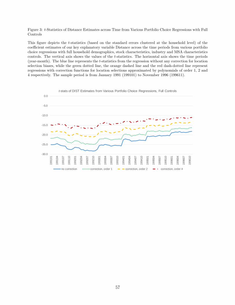
Figure 3: t-Statistics of Distance Estimates across Time from Various Portfolio Choice Regressions with FullControls

This figure depicts the t-statistics (based on the standard errors clustered at the household level) of thecoefficient estimates of our key explanatory variable Distance across the time periods from various portfoliochoice regressions with full household demographics, stock characteristics, industry and MSA characteristicscontrols. The vertical axis shows the values of the t-statistics. The horizontal axis shows the time periods(year-month). The blue line represents the t-statistics from the regression without any correction for locationselection biases, while the green dotted line, the orange dashed line and the red dash-dotted line representregressions with correction functions for location selections approximated by polynomials of order 1, 2 and4 respectively. The sample period is from January 1991 (199101) to November 1996 (199611).

-30.0

-25.0

-20.0

-15.0

-10.0

-5.0

0.0

19

9101

19

9104

19

9107

19

9110

19

9201

19

9204

19

9207

19

9210

19

9301

19

9304

19

9307

19

9310

19

9401

19

9404

19

9407

19

9410

19

9501

19

9504

19

9507

19

9510

19

9601

19

9604

19

9607

19

9610

t-stats of DIST Estimates from Various Portfolio Choice Regressions, Full Controls

no correction correction, order 1 correction, order 2 correction, order 4

57

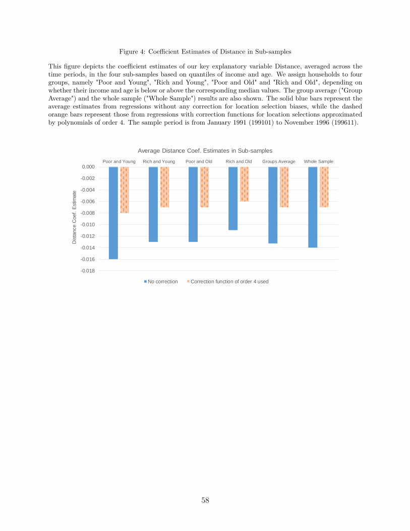
Figure 4: Coefficient Estimates of Distance in Sub-samples

This figure depicts the coefficient estimates of our key explanatory variable Distance, averaged across thetime periods, in the four sub-samples based on quantiles of income and age. We assign households to fourgroups, namely "Poor and Young", "Rich and Young", "Poor and Old" and "Rich and Old", depending onwhether their income and age is below or above the corresponding median values. The group average ("GroupAverage") and the whole sample ("Whole Sample") results are also shown. The solid blue bars represent theaverage estimates from regressions without any correction for location selection biases, while the dashedorange bars represent those from regressions with correction functions for location selections approximatedby polynomials of order 4. The sample period is from January 1991 (199101) to November 1996 (199611).

-0.018

-0.016

-0.014

-0.012

-0.010

-0.008

-0.006

-0.004

-0.002

0.000Poor and Young Rich and Young Poor and Old Rich and Old Groups Average Whole Sample

Dis

tance C

oef.

Estim

ate

Average Distance Coef. Estimates in Sub-samples

No correction Correction function of order 4 used

58

Internet Appendix For Online

Publication Only

59

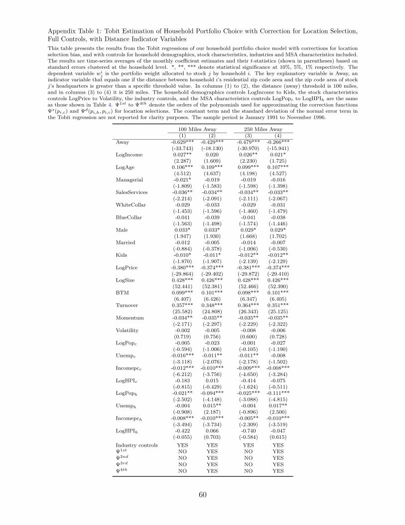
Appendix Table 1: Tobit Estimation of Household Portfolio Choice with Correction for Location Selection,Full Controls, with Distance Indicator VariablesThis table presents the results from the Tobit regressions of our household portfolio choice model with corrections for locationselection bias, and with controls for household demographics, stock characteristics, industries and MSA characteristics included.The results are time-series averages of the monthly coefficient estimates and their t-statistics (shown in parentheses) based onstandard errors clustered at the household level. *, **, *** denote statistical significance at 10%, 5%, 1% respectively. Thedependent variable wi

j is the portfolio weight allocated to stock j by household i. The key explanatory variable is Away, anindicator variable that equals one if the distance between household i’s residential zip code area and the zip code area of stockj’s headquarters is greater than a specific threshold value. In columns (1) to (2), the distance (away) threshold is 100 miles,and in columns (3) to (4) it is 250 miles. The household demographics controls LogIncome to Kids, the stock characteristicscontrols LogPrice to Volatility, the industry controls, and the MSA characteristics controls LogPopc to LogHPIh are the sameas those shown in Table 4. Ψ1st to Ψ4th denote the orders of the polynomials used for approximating the correction functionsΨs(pi,c) and Ψd(pi,h, pi,c) for location selections. The constant term and the standard deviation of the normal error term inthe Tobit regression are not reported for clarity purposes. The sample period is January 1991 to November 1996.

100 Miles Away 250 Miles Away(1) (2) (3) (4)

Away -0.629*** -0.429*** -0.479*** -0.266***(-33.743) (-18.130) (-30.970) (-15.941)

LogIncome 0.027** 0.020 0.026** 0.021*(2.287) (1.609) (2.230) (1.725)

LogAge 0.106*** 0.109*** 0.099*** 0.107***(4.512) (4.637) (4.198) (4.527)

Managerial -0.021* -0.019 -0.019 -0.016(-1.809) (-1.583) (-1.598) (-1.398)

SalesServices -0.036** -0.034** -0.034** -0.033**(-2.214) (-2.091) (-2.111) (-2.067)

WhiteCollar -0.029 -0.033 -0.029 -0.031(-1.453) (-1.596) (-1.460) (-1.479)

BlueCollar -0.041 -0.039 -0.041 -0.038(-1.563) (-1.498) (-1.574) (-1.446)

Male 0.033* 0.033* 0.029* 0.029*(1.947) (1.930) (1.668) (1.702)

Married -0.012 -0.005 -0.014 -0.007(-0.884) (-0.378) (-1.006) (-0.530)

Kids -0.010* -0.011* -0.012** -0.012**(-1.870) (-1.907) (-2.139) (-2.129)

LogPrice -0.380*** -0.374*** -0.381*** -0.374***(-29.864) (-29.402) (-29.872) (-29.410)

LogSize 0.428*** 0.426*** 0.428*** 0.426***(52.441) (52.381) (52.466) (52.390)

BTM 0.099*** 0.101*** 0.098*** 0.101***(6.407) (6.426) (6.347) (6.405)

Turnover 0.357*** 0.348*** 0.364*** 0.351***(25.582) (24.808) (26.343) (25.125)

Momentum -0.034** -0.035** -0.035** -0.035**(-2.171) (-2.297) (-2.229) (-2.322)

Volatility -0.002 -0.005 -0.008 -0.006(0.719) (0.756) (0.600) (0.728)

LogPopc -0.005 -0.023 -0.001 -0.027(-0.594) (-1.006) (-0.105) (-1.190)

Unempc -0.016*** -0.011** -0.011** -0.008(-3.118) (-2.076) (-2.178) (-1.502)

Incomepcc -0.012*** -0.010*** -0.009*** -0.008***(-6.212) (-3.756) (-4.650) (-3.284)

LogHPIc -0.183 0.015 -0.414 -0.075(-0.815) (-0.429) (-1.624) (-0.511)

LogPoph -0.021** -0.094*** -0.025*** -0.111***(-2.502) (-4.148) (-3.088) (-4.815)

Unemph -0.004 0.015** -0.004 0.017**(-0.908) (2.187) (-0.896) (2.500)

Incomepch -0.008*** -0.010*** -0.005** -0.010***(-3.494) (-3.734) (-2.309) (-3.519)

LogHPIh -0.422 0.066 -0.740 -0.047(-0.055) (0.703) (-0.584) (0.615)

Industry controls YES YES YES YESΨ1st NO YES NO YESΨ2nd NO YES NO YESΨ3rd NO YES NO YESΨ4th NO YES NO YES

60

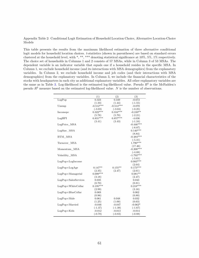
Appendix Table 2: Conditional Logit Estimation of Household Location Choice, Alternative Location-ChoiceModels

This table presents the results from the maximum likelihood estimation of three alternative conditionallogit models for household location choices. t-statistics (shown in parentheses) are based on standard errorsclustered at the household level, with *, **, *** denoting statistical significance at 10%, 5%, 1% respectively.The choice set of households in Columns 1 and 2 consists of 57 MSAs, while in Column 3 of 53 MSAs. Thedependent variable is an indicator variable that equals one if a household resides in the specific MSA. InColumn 1, we exclude household income (and its interactions with MSA demographics) from the explanatoryvariables. In Column 2, we exclude household income and job codes (and their interactions with MSAdemographics) from the explanatory variables. In Column 3, we include the financial characteristics of thestocks with headquarters in each city as additional explanatory variables. All other explanatory variables arethe same as in Table 3. Log-likelihood is the estimated log-likelihood value. Pseudo R2 is the McFadden’spseudo R2 measure based on the estimated log-likelihood value. N is the number of observations.

(1) (2) (3)LogPop 0.323 0.349 -0.672

(1.33) (1.44) (-1.55)Unemp -0.512*** -0.514*** -0.070

(-3.03) (-3.04) (-0.25)Incomepc 0.322*** 0.316*** -0.249**

(5.78) (5.70) (-2.21)LogHPI 6.831*** 6.857*** -4.636

(3.41) (3.43) (-1.34)LogPrice_MSA -0.446***

(-8.87)LogSize_MSA 0.140***

(8.84)BTM_MSA -0.484***

(-5.31)Turnover_MSA 1.790***

(17.46)Momentum_MSA -0.308***

(-4.08)Volatility_MSA -1.792***

(-5.61)LogPop×LogIncome 0.083***

(2.64)LogPop×LogAge 0.147** 0.155** 0.173***

(2.35) (2.47) (2.61)LogPop×Managerial 0.099*** 0.081**

(3.18) (2.47)LogPop×SalesServices 0.035 0.043

(0.70) (0.81)LogPop×WhiteCollar 0.195*** 0.218***

(2.99) (3.16)LogPop×BlueCollar 0.069 0.062

(0.96) (0.80)LogPop×Male 0.061 0.048 0.032

(1.25) (1.00) (0.63)LogPop×Married -0.046 -0.047 -0.062*

(-1.37) (-1.39) (-1.67)LogPop×Kids -0.012 -0.013 -0.014

(-0.78) (-0.83) (-0.88)

61

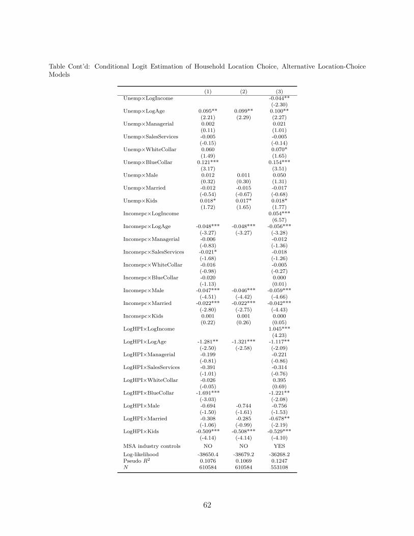
Table Cont’d: Conditional Logit Estimation of Household Location Choice, Alternative Location-ChoiceModels

(1) (2) (3)Unemp×LogIncome -0.044**

(-2.30)Unemp×LogAge 0.095** 0.099** 0.100**

(2.21) (2.29) (2.27)Unemp×Managerial 0.002 0.021

(0.11) (1.01)Unemp×SalesServices -0.005 -0.005

(-0.15) (-0.14)Unemp×WhiteCollar 0.060 0.070*

(1.49) (1.65)Unemp×BlueCollar 0.121*** 0.154***

(3.17) (3.51)Unemp×Male 0.012 0.011 0.050

(0.32) (0.30) (1.31)Unemp×Married -0.012 -0.015 -0.017

(-0.54) (-0.67) (-0.68)Unemp×Kids 0.018* 0.017* 0.018*

(1.72) (1.65) (1.77)Incomepc×LogIncome 0.054***

(6.57)Incomepc×LogAge -0.048*** -0.048*** -0.056***

(-3.27) (-3.27) (-3.28)Incomepc×Managerial -0.006 -0.012

(-0.83) (-1.36)Incomepc×SalesServices -0.021* -0.018

(-1.68) (-1.26)Incomepc×WhiteCollar -0.016 -0.005

(-0.98) (-0.27)Incomepc×BlueCollar -0.020 0.000

(-1.13) (0.01)Incomepc×Male -0.047*** -0.046*** -0.059***

(-4.51) (-4.42) (-4.66)Incomepc×Married -0.022*** -0.022*** -0.042***

(-2.80) (-2.75) (-4.43)Incomepc×Kids 0.001 0.001 0.000

(0.22) (0.26) (0.05)LogHPI×LogIncome 1.045***

(4.23)LogHPI×LogAge -1.281** -1.321*** -1.117**

(-2.50) (-2.58) (-2.09)LogHPI×Managerial -0.199 -0.221

(-0.81) (-0.86)LogHPI×SalesServices -0.391 -0.314

(-1.01) (-0.76)LogHPI×WhiteCollar -0.026 0.395

(-0.05) (0.69)LogHPI×BlueCollar -1.691*** -1.221**

(-3.03) (-2.08)LogHPI×Male -0.694 -0.744 -0.756

(-1.50) (-1.61) (-1.53)LogHPI×Married -0.308 -0.285 -0.678**

(-1.06) (-0.99) (-2.19)LogHPI×Kids -0.509*** -0.508*** -0.529***

(-4.14) (-4.14) (-4.10)MSA industry controls NO NO YESLog-likelihood -38650.4 -38679.2 -36268.2Pseudo R2 0.1076 0.1069 0.1247N 610584 610584 553108

62

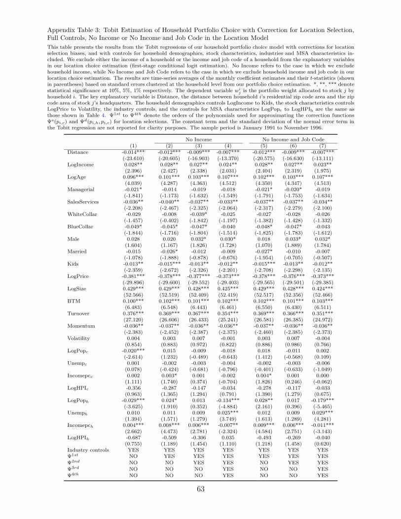
Appendix Table 3: Tobit Estimation of Household Portfolio Choice with Correction for Location Selection,Full Controls, No Income or No Income and Job Code in the Location ModelThis table presents the results from the Tobit regressions of our household portfolio choice model with corrections for locationselection biases, and with controls for household demographics, stock characteristics, industries and MSA characteristics in-cluded. We exclude either the income of a household or the income and job code of a household from the explanatory variablesin our location choice estimation (first-stage conditional logit estimation). No Income refers to the case in which we excludehousehold income, while No Income and Job Code refers to the case in which we exclude household income and job code in ourlocation choice estimation. The results are time-series averages of the monthly coefficient estimates and their t-statistics (shownin parentheses) based on standard errors clustered at the household level from our portfolio choice estimation. *, **, *** denotestatistical significance at 10%, 5%, 1% respectively. The dependent variable wi

j is the portfolio weight allocated to stock j byhousehold i. The key explanatory variable is Distance, the distance between household i’s residential zip code area and the zipcode area of stock j’s headquarters. The household demographics controls LogIncome to Kids, the stock characteristics controlsLogPrice to Volatility, the industry controls, and the controls for MSA characteristics LogPopc to LogHPIh are the same asthose shown in Table 4. Ψ1st to Ψ4th denote the orders of the polynomials used for approximating the correction functionsΨs(pi,c) and Ψd(pi,h, pi,c) for location selections. The constant term and the standard deviation of the normal error term inthe Tobit regression are not reported for clarity purposes. The sample period is January 1991 to November 1996.

No Income No Income and Job Code(1) (2) (3) (4) (5) (6) (7)

Distance -0.014*** -0.012*** -0.009*** -0.007*** -0.012*** -0.009*** -0.007***(-23.610) (-20.605) (-16.903) (-13.370) (-20.575) (-16.630) (-13.111)

LogIncome 0.028** 0.028** 0.027** 0.024** 0.028** 0.027** 0.023**(2.396) (2.427) (2.338) (2.031) (2.404) (2.319) (1.975)

LogAge 0.096*** 0.101*** 0.103*** 0.107*** 0.102*** 0.103*** 0.107***(4.039) (4.287) (4.363) (4.512) (4.350) (4.347) (4.513)

Managerial -0.021* -0.014 -0.019 -0.018 -0.021* -0.020* -0.019(-1.841) (-1.173) (-1.632) (-1.549) (-1.791) (-1.753) (-1.634)

SalesServices -0.036** -0.040** -0.037** -0.033** -0.037** -0.037** -0.034**(-2.208) (-2.467) (-2.325) (-2.064) (-2.317) (-2.279) (-2.100)

WhiteCollar -0.029 -0.008 -0.039* -0.025 -0.027 -0.028 -0.026(-1.457) (-0.402) (-1.842) (-1.197) (-1.382) (-1.428) (-1.332)

BlueCollar -0.049* -0.045* -0.047* -0.040 -0.048* -0.047* -0.043(-1.844) (-1.716) (-1.804) (-1.514) (-1.825) (-1.783) (-1.612)

Male 0.028 0.020 0.032* 0.030* 0.018 0.033* 0.032*(1.604) (1.167) (1.826) (1.728) (1.070) (1.889) (1.784)

Married -0.015 -0.026* -0.012 -0.009 -0.027* -0.010 -0.007(-1.078) (-1.888) (-0.878) (-0.676) (-1.954) (-0.705) (-0.507)

Kids -0.013** -0.015*** -0.013** -0.012** -0.015*** -0.013** -0.012**(-2.359) (-2.672) (-2.326) (-2.201) (-2.708) (-2.298) (-2.135)

LogPrice -0.381*** -0.378*** -0.377*** -0.373*** -0.378*** -0.376*** -0.373***(-29.896) (-29.600) (-29.552) (-29.403) (-29.565) (-29.501) (-29.385)

LogSize 0.429*** 0.429*** 0.428*** 0.425*** 0.429*** 0.428*** 0.424***(52.566) (52.519) (52.409) (52.419) (52.517) (52.356) (52.466)

BTM 0.100*** 0.102*** 0.101*** 0.102*** 0.102*** 0.101*** 0.103***(6.483) (6.548) (6.443) (6.461) (6.550) (6.430) (6.511)

Turnover 0.376*** 0.369*** 0.367*** 0.354*** 0.369*** 0.366*** 0.351***(27.120) (26.606) (26.433) (25.241) (26.581) (26.385) (24.972)

Momentum -0.036** -0.037** -0.036** -0.036** -0.037** -0.036** -0.036**(-2.383) (-2.452) (-2.387) (-2.375) (-2.460) (-2.385) (-2.373)

Volatility 0.004 0.003 0.007 -0.001 0.003 0.007 -0.004(0.854) (0.883) (0.972) (0.822) (0.886) (0.986) (0.766)

LogPopc -0.020*** 0.015 -0.009 -0.018 0.018 -0.011 0.002(-2.614) (1.232) (-0.489) (-0.643) (1.412) (-0.568) (0.109)

Unempc 0.001 -0.002 -0.003 -0.004 -0.002 -0.003 -0.006(0.078) (-0.424) (-0.681) (-0.796) (-0.401) (-0.633) (-1.049)

Incomepcc 0.002 0.003* 0.001 -0.002 0.004* 0.001 0.000(1.111) (1.740) (0.374) (-0.704) (1.826) (0.246) (-0.062)

LogHPIc -0.356 -0.287 -0.147 -0.034 -0.278 -0.117 -0.033(0.963) (1.365) (1.294) (0.791) (1.390) (1.279) (0.675)

LogPoph -0.029*** 0.024* 0.013 -0.134*** 0.028** 0.017 -0.179***(-3.625) (1.910) (0.352) (-4.884) (2.161) (0.396) (-5.465)

Unemph 0.010 0.011 0.009 0.025*** 0.012 0.009 0.029***(1.394) (1.571) (1.279) (3.749) (1.613) (1.289) (4.281)

Incomepch 0.004*** 0.008*** 0.006*** -0.007** 0.009*** 0.006*** -0.011***(2.662) (4.473) (2.781) (-2.324) (4.584) (2.751) (-3.143)

LogHPIh -0.687 -0.509 -0.306 0.035 -0.493 -0.269 -0.040(0.755) (1.189) (1.454) (1.110) (1.218) (1.458) (0.620)

Industry controls YES YES YES YES YES YES YESΨ1st NO YES YES YES YES YES YESΨ2nd NO NO YES YES NO YES YESΨ3rd NO NO NO YES NO NO YESΨ4th NO NO NO YES NO NO YES

63

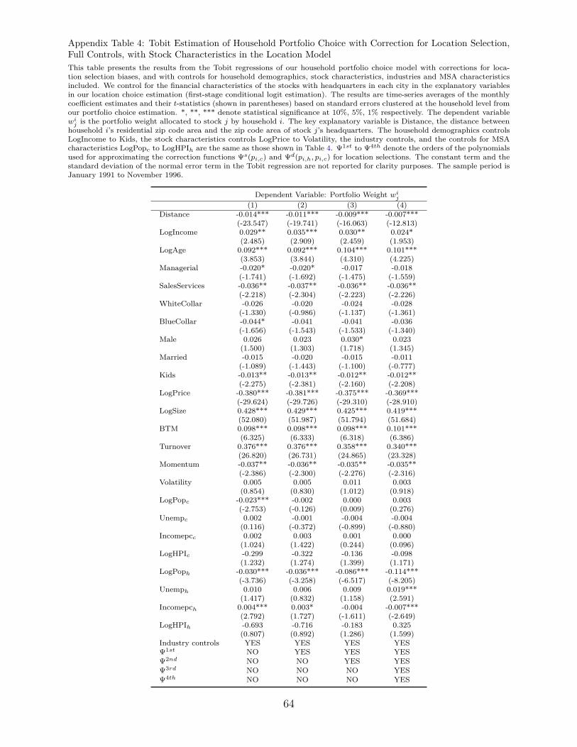
Appendix Table 4: Tobit Estimation of Household Portfolio Choice with Correction for Location Selection,Full Controls, with Stock Characteristics in the Location ModelThis table presents the results from the Tobit regressions of our household portfolio choice model with corrections for loca-tion selection biases, and with controls for household demographics, stock characteristics, industries and MSA characteristicsincluded. We control for the financial characteristics of the stocks with headquarters in each city in the explanatory variablesin our location choice estimation (first-stage conditional logit estimation). The results are time-series averages of the monthlycoefficient estimates and their t-statistics (shown in parentheses) based on standard errors clustered at the household level fromour portfolio choice estimation. *, **, *** denote statistical significance at 10%, 5%, 1% respectively. The dependent variablewi

j is the portfolio weight allocated to stock j by household i. The key explanatory variable is Distance, the distance betweenhousehold i’s residential zip code area and the zip code area of stock j’s headquarters. The household demographics controlsLogIncome to Kids, the stock characteristics controls LogPrice to Volatility, the industry controls, and the controls for MSAcharacteristics LogPopc to LogHPIh are the same as those shown in Table 4. Ψ1st to Ψ4th denote the orders of the polynomialsused for approximating the correction functions Ψs(pi,c) and Ψd(pi,h, pi,c) for location selections. The constant term and thestandard deviation of the normal error term in the Tobit regression are not reported for clarity purposes. The sample period isJanuary 1991 to November 1996.

Dependent Variable: Portfolio Weight wij

(1) (2) (3) (4)Distance -0.014*** -0.011*** -0.009*** -0.007***

(-23.547) (-19.741) (-16.063) (-12.813)LogIncome 0.029** 0.035*** 0.030** 0.024*

(2.485) (2.909) (2.459) (1.953)LogAge 0.092*** 0.092*** 0.104*** 0.101***

(3.853) (3.844) (4.310) (4.225)Managerial -0.020* -0.020* -0.017 -0.018

(-1.741) (-1.692) (-1.475) (-1.559)SalesServices -0.036** -0.037** -0.036** -0.036**

(-2.218) (-2.304) (-2.223) (-2.226)WhiteCollar -0.026 -0.020 -0.024 -0.028

(-1.330) (-0.986) (-1.137) (-1.361)BlueCollar -0.044* -0.041 -0.041 -0.036

(-1.656) (-1.543) (-1.533) (-1.340)Male 0.026 0.023 0.030* 0.023

(1.500) (1.303) (1.718) (1.345)Married -0.015 -0.020 -0.015 -0.011

(-1.089) (-1.443) (-1.100) (-0.777)Kids -0.013** -0.013** -0.012** -0.012**

(-2.275) (-2.381) (-2.160) (-2.208)LogPrice -0.380*** -0.381*** -0.375*** -0.369***

(-29.624) (-29.726) (-29.310) (-28.910)LogSize 0.428*** 0.429*** 0.425*** 0.419***

(52.080) (51.987) (51.794) (51.684)BTM 0.098*** 0.098*** 0.098*** 0.101***

(6.325) (6.333) (6.318) (6.386)Turnover 0.376*** 0.376*** 0.358*** 0.340***

(26.820) (26.731) (24.865) (23.328)Momentum -0.037** -0.036** -0.035** -0.035**

(-2.386) (-2.300) (-2.276) (-2.316)Volatility 0.005 0.005 0.011 0.003

(0.854) (0.830) (1.012) (0.918)LogPopc -0.023*** -0.002 0.000 0.003

(-2.753) (-0.126) (0.009) (0.276)Unempc 0.002 -0.001 -0.004 -0.004

(0.116) (-0.372) (-0.899) (-0.880)Incomepcc 0.002 0.003 0.001 0.000

(1.024) (1.422) (0.244) (0.096)LogHPIc -0.299 -0.322 -0.136 -0.098

(1.232) (1.274) (1.399) (1.171)LogPoph -0.030*** -0.036*** -0.086*** -0.114***

(-3.736) (-3.258) (-6.517) (-8.205)Unemph 0.010 0.006 0.009 0.019***

(1.417) (0.832) (1.158) (2.591)Incomepch 0.004*** 0.003* -0.004 -0.007***

(2.792) (1.727) (-1.611) (-2.649)LogHPIh -0.693 -0.716 -0.183 0.325

(0.807) (0.892) (1.286) (1.599)Industry controls YES YES YES YESΨ1st NO YES YES YESΨ2nd NO NO YES YESΨ3rd NO NO NO YESΨ4th NO NO NO YES

64