Locating Faults by the Traveling Waves They Launch

Locating Faults by the Traveling Waves They Launch

Edmund O. Schweitzer, III, Armando Guzmán, Mangapathirao V. Mynam, Veselin Skendzic, and Bogdan Kasztenny Schweitzer Engineering Laboratories, Inc.

Stephen Marx Bonneville Power Administration

© 2014 IEEE. Personal use of this material is permitted. Permission from IEEE must be obtained for all other uses, in any current or future media, including reprinting/republishing this material for advertising or promotional purposes, creating new collective works, for resale or redistribution to servers or lists, or reuse of any copyrighted component of this work in other works.

This paper was presented at the 67th Annual Conference for Protective Relay Engineers and can be accessed at: http://dx.doi.org/10.1109/CPRE.2014.6798997.

For the complete history of this paper, refer to the next page.

Published in Locating Faults and Protecting Lines at the

Speed of Light: Time-Domain Principles Applied, 2018

Previously presented at the 50th Annual Minnesota Power Systems Conference, November 2014,

5th Annual Protection, Automation and Control World Conference, June 2014, 17th Annual Georgia Tech Fault and Disturbance Analysis Conference, April 2014,

and 67th Annual Conference for Protective Relay Engineers, March 2014

Previously published in Line Current Differential Protection: A Collection of

Technical Papers Representing Modern Solutions, 2014

Originally presented at the 40th Annual Western Protective Relay Conference, October 2013

1

Locating Faults by the Traveling Waves They Launch

Edmund O. Schweitzer, III, Armando Guzmán, Mangapathirao V. Mynam, Veselin Skendzic, and Bogdan Kasztenny, Schweitzer Engineering Laboratories, Inc.

Stephen Marx, Bonneville Power Administration

Abstract—Faults on overhead transmission lines cause transients that travel at the speed of light and propagate along the power line as traveling waves (TWs). This paper provides an overview of TWs and TW fault locators. It explains the physics, reviews the theory of TWs, explains the foundations of various types of TW fault locators, and provides an in-depth discussion on a number of TW fault locating implementation challenges. Finally, it discusses integration of TW fault locating in microprocessor-based relays and presents Bonneville Power Administration’s (BPA’s) field experience using these relays.

I. INTRODUCTION

Fast and accurate fault locating of both permanent and temporary faults on transmission lines is of great value to power transmission asset owners and operators. Fault locating as a discipline dates back to the 1940s and continues to evolve.

Visual inspection methods evolved from road to air patrols and, more recently, to trials with unmanned aerial vehicles. To aid in the visual inspection process, tower targets were introduced [1] [2]. In [1], a target, activated by a gun powder cartridge, was installed on each tower. As the fault current traveled to ground through the tower, it would heat up the charge and set the target pointing to the fault location. This approach significantly helped ground patrols identify damaged insulators.

Fault locating using electrical measurements evolved from simple electromechanical devices to microprocessor-based systems integrated with geospatial data.

One electromechanical device, an annunciator ammeter, is shown in Fig. 1 [3]. Using the fault current level from the meter, an approximate fault location was calculated based on system and line parameters, with the estimated error in the range of 20 percent of the line length.

Fig. 1. Westinghouse JM Group Annunciator and Current Indicator.

Automatic oscillographs were an improvement over annunciator ammeters because the oscillographs used both current and voltage signals and provided accuracy of around 10 percent [4].

Another family of early fault locators used active injection to locate permanent faults. A pulse radar method [5] would send a short pulse (such as 1 µs, 10 kV) into the faulted line after the breaker opened and measure the travel time to and from the fault. The pulse travel time was subsequently converted into physical distance with an expected accuracy of better than 1 percent. Another approach, a resonance method, applied a series of frequencies to effectively measure the frequency response of the faulted line. The fault location was deduced from the frequency response plot. This method had an expected accuracy of 2 to 5 percent [6].

Impedance-based fault locating uses voltage and current measurements at system frequency, i.e., the sinusoidal quasi-steady-state “phasor” quantities combined with different assumptions about the power system to dramatically improve accuracy over the automatic oscillograph method.

Different assumptions lead to a variety of impedance-based fault locating methods. For example, the assumption that the fault current at the fault location is in phase with the fault component of the current at the line terminal led to the Takagi method [7]. Observing that the fault current at the fault location is effectively in phase with the negative-sequence current at the line terminal led to the Schweitzer method [8]. The method used in [8] was the first fault locating method integrated into protective relays. This integration accelerated deployment of digital fault locating by making it more practical, convenient, and essentially free.

Over the years, several different impedance-based methods have been pursued, using information from one or both line ends. All these impedance-based methods, however, face accuracy limitations, including nonhomogeneity of the transmission line, uncertainty of the line impedance data, mutual coupling, series compensation, variability of the arc resistance during the fault, transients, taps, limited voltage and current data between fault inception and breaker operation, limited accuracy of instrument transformers, and ground potential rise for close-in faults.

As a result, accuracy of the impedance-based fault locators is in the order of 0.5 to 2 percent. For a 300 km transmission line, a ±1 percent error still leaves a 6 km section to be patrolled (about 20 towers).

2

Traveling wave (TW) methods use the naturally occurring surges and waves that are generated by the fault. Bonneville Power Administration (BPA) has been a pioneer in TW fault locating, with the first implementations dating back to the 1940s (see Fig. 2). Initially, TW fault locating required only a few technologies that were relatively easy to implement, namely: ability to measure, filter, and amplify the surges; measure time with microsecond accuracy; and communicate with a relatively constant latency. The TW fault locating methods can approach accuracy of 300 m, or about one tower span.

Fig. 2. TW fault locator at BPA, circa 1948 [9].

Advancements in the technology, especially high-speed sampling, digital signal processing, satellite-based synchronization, and digital communications, enable further improvements in TW fault locating. TW fault locating has recently been integrated with microprocessor-based line protection relays [10], improving convenience and reducing cost of ownership to utilities.

II. TW FAULT LOCATING METHODS

A fault at any point on the voltage wave other than at voltage zero launches a step wave, which propagates in both directions from the fault location as shown in Fig. 3 (in the unlikely case of a fault at voltage zero, a ramp wave is launched). One method of determining the fault location uses precise measures of the TW arrival times at both ends of the transmission line.

Fig. 3. TWs propagate in both directions away from the fault.

In early implementations, the time of arrival at one line end was conveyed to the other end over a wide bandwidth communications channel, such as microwave baseband, and the communications delay was accounted for in the time difference measurement. Fig. 4 shows a representation of BPA’s 1955 TW fault locating system for their 500 kV ac transmission network. This two-end system used microwave communication to send a pulse from the remote terminal to signal the TW arrival time.

L

Counter

Start

Stop

Microwave Receiver

TW Processing

Unit

Microwave Transmitter

Master Terminal Remote Terminal

Wave R

R

Wave L

TW Processing

Unit

Fig. 4. TW fault locating operation based on time of arrival conveyed via microwave channel [11].

The TW reaching the master terminal starts an electronic counter. The remote terminal sends a stop pulse to the master terminal via the microwave channel when the TW reaches the remote terminal (see Fig. 4). The TW fault locator determines the counter time, compensates for the communications delay, and translates this time to the fault distance, m, from the master terminal as follows:

Timer Channel1

m t t • v2 (1)

where:

ℓ is the line length.

tTimer is the counter elapsed time. tChannel is the communications channel delay (assumed longer than the line propagation time). v is the TW propagation velocity.

Modern TW fault locators using a common time reference for the devices capturing the TWs at the line terminals are, in principle, simple. This TW fault locating approach, shown in Fig. 5, is known as Type D.

Fig. 5. Fault locating principle of operation using a common time reference.

In Type D TW fault locating, the required wave arrival times are measured with a common time reference and are exchanged in order to calculate the fault location as follows:

L R

1m t t • v

2 (2)

where: is the line length. tL is the TW arrival time at L. tR is the TW arrival time at R. v is the TW propagation velocity.

3

This method leverages the economical and broadly available technologies of digital communications and satellite-based time synchronization. Most recently, digital communications devices designed for critical infrastructure provide absolute time over a wide-area network, independent of Global Positioning Systems (GPS) [12]. Terrestrial communications have the advantage over GPS of being less susceptible to jamming or spoofing.

Type D fault locating technology can be further illustrated using the Bewley lattice diagram as shown in Fig. 6 that shows a line connecting two buses, L and R, with networks behind each bus. A fault at distance m from L launches TWs toward L and R. If the fault is in the middle of the line, then the TW reaches L and R at the same absolute time, so the relative time of arrival is zero. We drew Fig. 6 with m < – m, so the TW reaches L before R. The energy of the incident TW reaching L divides three ways: some reflects back toward the fault, some transmits through L, and some is absorbed. Of course, similar things happen at R, only a bit later in this case.

The first thing known at L about the fault is the initial arrival of the TW from the fault at time tL1, and the first thing known at R about the fault is the initial arrival of the TW from the fault at time tR1. Two-end fault locating methods use these first TW arrival times and do not rely on subsequent TW reflections.

Another TW fault locating method uses TW information from one end of the line and eliminates need for precise relative timing and communications. Referring to Fig. 6 again, we see the TW reaching L is both transmitted and reflected. The reflected energy bounces off the fault (some is transmitted toward R) and eventually travels back to L, arriving at time tL2. The time tL2 – tL1 is the travel time from L to the fault and back.

Fig. 6. Lattice diagram showing incident, reflected, and transmitted TWs.

To estimate fault location, this single-end fault locating method uses the time difference between the first arrived TW and the successive reflection from the fault, as shown in (3).

L2 L1t tm • v

2

(3)

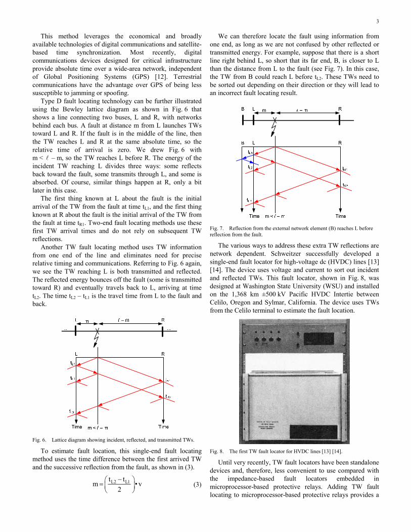
We can therefore locate the fault using information from one end, as long as we are not confused by other reflected or transmitted energy. For example, suppose that there is a short line right behind L, so short that its far end, B, is closer to L than the distance from L to the fault (see Fig. 7). In this case, the TW from B could reach L before tL2. These TWs need to be sorted out depending on their direction or they will lead to an incorrect fault locating result.

Fig. 7. Reflection from the external network element (B) reaches L before reflection from the fault.

The various ways to address these extra TW reflections are network dependent. Schweitzer successfully developed a single-end fault locator for high-voltage dc (HVDC) lines [13] [14]. The device uses voltage and current to sort out incident and reflected TWs. This fault locator, shown in Fig. 8, was designed at Washington State University (WSU) and installed on the 1,368 km ±500 kV Pacific HVDC Intertie between Celilo, Oregon and Sylmar, California. The device uses TWs from the Celilo terminal to estimate the fault location.

Fig. 8. The first TW fault locator for HVDC lines [13] [14].

Until very recently, TW fault locators have been standalone devices and, therefore, less convenient to use compared with the impedance-based fault locators embedded in microprocessor-based protective relays. Adding TW fault locating to microprocessor-based protective relays provides a

4

superior fault locating system by combining both the impedance-based and TW fault locating methods.

III. TW PHENOMENA IN POWER LINES

Power system faults result from the unintended breakdown of insulation. At the very instant of the fault, the current is only supplied locally from the charge stored in the line capacitance. At the same instant, a remote observer performing measurements at the line terminal (substation) has no way of knowing that the fault has occurred. Information about the fault, which propagates very close to the speed of light, travels down the line and reaches the observer.

The TWs reach the line terminals and are transmitted and reflected depending on the relative values of the characteristic impedances of the line and the adjacent network components. Fig. 9 shows the TW reflections and their corresponding attenuation as time progresses. The TW signals in Fig. 9 were obtained by filtering the phase currents and voltages during a fault using a high-pass filter with a cutoff frequency of 2 kHz.

Faults launch waves having energy over a wide frequency spectrum. The energy useful for TW fault locating is mostly present in the 20 kHz to 2 MHz range [10].

0.3 0.301 0.302 0.303 0.304 0.305 0.306 0.307 0.30

Fig. 9. High-frequency transient component for typical fault current and voltage waveforms where Phase A is red, Phase B is green, and Phase C is blue.

In this section we derive, discuss, and illustrate the basic theory of TWs in three-phase power lines.

A. Line Equations for Two Conductors in Free Space

Fig. 10 shows the equivalent circuit of a segment with length ∆x of a two-conductor transmission line. The circuit includes the resistance R, inductance L, conductance G, and capacitance C of the line in per unit of line length [15].

Fig. 10. Equivalent circuit of a segment of a two-conductor transmission line.

We use Kirchhoff’s voltage law, shown in (4), and Kirchhoff’s current law, shown in (5), to relate the voltages and currents at locations x and x + Δx.

v x, t v x x, t

i x, tR • x • i x, t L • x

t

(4)

i x, t i x x, t

v x x, tG • x • v x x, t C • x

t

(5)

We can divide both sides of (4) and (5) by the line segment length Δx to obtain the rate of change of the voltage and current for a change in location Δx. If we assume the change in location Δx approaches zero, we will obtain derivatives of the voltage and current with respect to the position x as shown in (6) and (7). These equations determine the voltage and current as a function of location (x) and time (t) for the two-conductor transmission line. The negative signs indicate that the amplitudes of the waves decrease as x increases.

v x, t i x, t

R • i x, t Lx t

(6)

i x, t v x, t

G • v x, t Cx t

(7)

We substitute the Heaviside operator:

st

in (6) and (7) to transform these equations from the time domain into the Laplace domain as shown in (8) and (9) [16].

v x,sR sL • i x,s

x

(8)

i x,sG sC • v x,s

x

(9)

We further introduce Z = R + sL and Y = G + sC and use them to obtain (10) and (11).

v x,sZ • i x,s

x

(10)

i x,sY • v x,s

x

(11)

Our goal is to have two separate equations that would involve only the voltage and only the current, but not both. We can accomplish this if we take the derivative of (10) and (11) with respect to x to obtain (12) and (13).

2

2

v x,s i x,sZ •

xx

(12)

2

2

i x,s v x,sY •

xx

(13)

5

We then substitute (10) and (11) into (12) and (13) to obtain the voltage and current wave equations (14) and (15).

2

2

v x,sZ• Y • v x,s

x

(14)

2

2

i x,sY • Z• i x,s

x

(15)

Equation (16) defines the propagation constant γ, and (17) and (18) are the wave equations that include γ.

Z • Y (16)

22

2

v x,s• v x,s 0

x

(17)

22

2

i x,s• i x,s 0

x

(18)

Equations (17) and (18) describe the TWs in the Laplace domain. Solving these equations requires assuming a disturbance, such as a step change in voltage caused by a fault, and a set of boundary conditions, such as an open line terminal (current is zero) or a transition point to a bus. Before we can discuss any specific TWs, let us look at the general solutions of the TW equations, irrespective of the boundary conditions.

Equations (19) and (20) are the general solutions for the second-order partial differential equations (17) and (18). The voltage and current are the sum of two components; these components are referred to as the incident wave vIe

–γx, iIe–γx

and the reflected wave vReγx, iReγx.

x xI Rv x, t v e v e (19)

x xI Ri x, t i e i e (20)

When we look at voltage and current from a given point on the transmission line, we can calculate the ratio between the voltage and current for the incident and the reflected components, respectively; these ratios depend on the line parameters and define the line characteristic impedance as shown in (21) and (22).

IC

I

v ZZ

i Y (21)

RC

R

v ZZ –

i Y (22)

Equation (23) expresses i(x,t) as a function of vI, vR, and ZC.

x xI R

C

1i x, t v e – v e

Z (23)

Now let us examine what happens when a TW reaches a discontinuity, i.e., a point when the characteristic impedance of the circuit changes.

B. Terminations

A fault launches waves in both directions, which propagate from the fault toward the line terminals. The TW consists of a

voltage and a current component, related by the characteristic impedance of the line (21) and (22). When an incident TW with current (iI) and voltage (vI) reaches a line terminal, a portion of the incident TW is transmitted, (iT) and (vT), and the remaining portion is reflected, (iR) and (vR). The amount of energy that is transmitted and reflected depends on the characteristic impedance beyond the transition point (ZT) and the characteristic impedance (ZC) of the line the wave traveled, as shown in Fig. 11. A device at the line terminal measures current and voltage values that are the sum of the incident and reflected TWs.

Fig. 11. Illustration of the incident (iI), transmitted (iT), and reflected (iR) waves.

When a surge reaches termination impedance (ZT) at the terminal, the voltage (v) at the terminal equals iZT. The arrival of iI and vI at the terminal creates reflected TWs (iR) and (vR) according to (24).

I RT

I R

v vvZ

i i i

(24)

Our objective is to define a relationship between the incident and reflected TWs. Therefore, we substitute (21) and (22) into (24), and we obtain (25), which is the reflected TW voltage as a function of vI, ZC, and ZT.

T CR I v I

T C

Z Zv v v

Z Z

(25)

where v is the voltage reflection coefficient. Similarly, we can obtain the current reflection coefficient

I expressed in (26).

C TI

T C

Z Z

Z Z

(26)

Equations (25) and (26) tell us how the TW energy in the voltage and in the current divides between the incident and reflected TWs. For example, if ZC = ZT, no energy is reflected and all energy is transmitted. If ZT = 0, the reflected TW voltage equals the incident TW voltage (with the opposite sign) and no energy is transmitted. If ZT = ∞, the reflected TW current equals the incident TW current (with the opposite sign) and no energy is transmitted. We can separate the incident and reflected TWs when we measure both current and voltage at the line terminal. We will return to this discussion in Subsection F.

C. Attenuation and Losses

A fault or a lightning strike generates a surge in voltage and current. The associated TWs attenuate as they propagate along the line because of losses caused by the line resistance and conductance.

To analyze the propagation of TWs in systems with transmission lines having multiple conductors, we perform

6

modal analysis to decouple the wave propagation modes [17]. In modal analysis, the phase signals are linear combinations of the mode signals, and vice versa, as further explained in Subsection D. These linear combinations are expressed by the following transformation matrices.

Phase i ModeI T I (27)

Phase v ModeV T V (28)

–1Mode i PhaseI T I (29)

–1Mode v PhaseV T V (30)

In the analysis of a multiconductor line, the R, L, G, and C parameters of the transmission line are matrices with dimensions according to the number of conductors (n). The same applies to Z, Y, and values in the TW line model (17) and (18). Consider the propagation matrices Av in (31) and Ai in (32), where Z and Y are the impedance and admittance matrices of the line.

vA ZY (31)

iA YZ (32)

Our goal is to establish how the TWs would propagate once they occur. This is normally done using eigenvalue analysis. We will ideally select the transformation matrices Ti and Tv so that the following matrix (is diagonal, meaning the modes are decoupled.

1v v vT A T (33)

1i i iT A T (34)

1

n

0

0

(35)

The square root of each eigenvalue (m) in represents the wave propagation constant (m) for the corresponding mode m.

m m (36)

The real part (m) in (37), represents the attenuation constant, and the imaginary part (m) represents the phase constant of the propagation constant (m).

m m mj (37)

Equation (37) has a two-fold significance. First, the nonzero value of its real part means that the wave magnitude reduces as it travels along the line. This attenuation illustrates that transmission lines have losses resulting from the resistance (R) and conductance (G) of the line. Second, the nonzero value of the imaginary part in (37) shows that the propagation velocity (vm) of a particular mode (m) depends on the frequency (:

mm

v

(38)

For a lossless line, the propagation velocity is constant and dictated by the inductance (L) and capacitance (C) of the line. Equation (37) also shows that each mode may have unique attenuation and propagation velocity.

A different way to look at the dependence of propagation velocity on frequency is to look at the steepness of the TW rising edge in the time domain. If the TW is launched as an ideal step, it contains an infinite spectrum of frequencies. The frequency components propagate at different velocities per (38), causing the initial step in the TW to become distorted. When observed at some distance away from the fault, the TW edge will lean more and more as it travels along the line. This phenomenon is referred to as dispersion or distortion.

Dispersion is of particular interest for TW fault locating because the steepness of the TW rising edge can impact the estimation of the TW arrival time.

As mentioned earlier, dispersion can be different for different modes in a multiconductor system. Let us now examine the Clarke transformation, which is a true modal decomposition.

D. Modal Analysis

In addition to analyzing power systems using phase currents and voltages, we often rely on an auxiliary set of variables obtained from the phase currents and voltages via a linear transformation of choice. These transformations are selected to simplify the analysis by taking advantage of specific relationships between the parameters in the three-phase system or specific relationships between the phase signals. Symmetrical components are the most common transformation used in power system analysis, fault analysis in particular. However, symmetrical components apply to current and voltage phasors and not to instantaneous values such as current and voltage TWs. To analyze TWs, we use the Clarke transformation [18]. Equation (39) defines the Clarke components of the phase currents, with reference to Phase A.

0 A A

1c B B

C C

I I 1 1 1 I1

I T I 2 1 1 I3

I I I0 3 3

(39)

The three modes are referred to as zero, alpha, and beta. If equal currents flow down the A, B, and C conductors and return in the earth, then only the zero mode, shown in the top row of (39), is excited. If all of the current flows down Phase A and half returns on B and C, then only the alpha mode is excited, shown in the middle row of (39). If all current flows down B and returns on C, then only the beta mode is excited.

The Clarke components calculated with reference to Phase A work well for AG and BC faults but will not work optimally for other fault types.

7

In order to cover all fault types, we can use three sets of Clarke components with reference to Phase A, Phase B, and Phase C as follows:

A

AA

B

AC0

2 1 1I I1

I 0 3 3 I3

1 1 1 II

(40)

B

AB

B

BC0

1 2 1I I1

I 3 0 3 I3

1 1 1 II

(41)

C

AC

B

CC0

1 1 2I I1

I 3 3 0 I3

1 1 1 II

(42)

The need to work with three sets of Clarke components makes them less convenient to use compared with symmetrical components when analyzing frequency-domain signals (phasors). Because symmetrical components cannot be used to analyze TW transients, we have to rely on Clarke components, despite the need for three sets of calculations. The alpha components are appropriate for analyzing TWs launched by SLG faults and the beta components for LL faults.

The characteristic impedances, attenuation, and dispersion are in general different for the three modes. Propagation velocity, dispersion, and attenuation are key criteria when selecting the mode for TW fault locating.

E. Mode and Phase Reference Selection

The zero-sequence mode is the least appropriate for TW fault locating, because it has more attenuation and dispersion than the aerial alpha and beta modes, due to greater losses in the earth than in the conductors. This leaves six aerial Clarke components to work with: alpha and beta, each referenced to Phases A, B, or C. Simulations show that alpha and beta components have the following characteristics:

The alpha currents are available for all fault types. They provide a reliable quantity to detect TWs.

The beta currents provide marginally higher signal magnitudes for phase-to-phase faults when the phase-to-phase voltage difference at the fault location is higher than the phase-to-ground voltages of the faulted phases.

Using the highest of the alpha and beta currents reduces the fault location estimation error, but only marginally and only in some cases.

As a result of our findings, our implementation uses the alpha component with the largest amplitude.

F. Separation of Incident and Reflected Waves

TWs measured at the device location are a superposition of the incident and reflected waves, as explained earlier in Subsection B. It is possible to separate the incident and reflected waves.

Let us obtain the incident voltage at the remote end (vI) as a function of the measured terminal voltage (v) and terminal current (i). Equations (43) and (44) represent v and i in terms of their corresponding incident and reflected waves.

I Rv v v (43)

I Ri i i (44)

Then in (45) we express i in terms of vI and vR, and in (46) we solve (45) for vR.

I R

C C

v vi

Z Z (45)

R I Cv v iZ (46)

We substitute vR from (46) into (43) and solve for vI to obtain (47), which expresses the voltage of the incident wave at the line terminal as a function of the voltage and current measured at the terminal.

CI

v iZv

2

(47)

In a similar way, we obtain (48), which expresses the voltage of the reflected wave at the line terminal as a function of v and i.

CR

v iZv

2

(48)

Operations (47) and (48) are performed on modal currents and voltages using the corresponding characteristic impedance of the line. The challenge in separating the incident and reflected waves is proper measurement of voltages and currents at the line terminals. The design of current transformers (CTs) and voltage transformers (VTs) has been optimized for nominal frequency operation. TW signals can be measured using specialized high-frequency transducers similar to those used in high-voltage laboratories, but the high cost and custom nature of these devices make this approach impractical for wide-scale utility applications.

It is more convenient if the TW fault locating device is installed in the substation control house using conventional wiring and existing instrument transformers. Common choices for voltage and current measurements on high-voltage transmission lines are coupling capacitor voltage transformers (CCVTs) and conventional CTs.

CCVTs have a poor frequency response [19] [20]. They are tuned to the nominal signal frequency and show very large attenuation for frequencies in the kHz and MHz range. They are not generally suitable for TW measurement using their standard secondary voltage outputs. We may tap the low-voltage stack of the capacitive divider (power line carrier interface terminal) in order to measure TWs in line voltages, but this application requires extra wiring and interface and is not convenient.

Because of the practical limitations of CCVTs, we decided to use currents for TW fault locating. Conventional CTs have a good high-frequency response [21]. The usable passband easily reaches 100 kHz [21] and may often be closer to the 200 kHz [22] or 500 kHz [23] level.

8

Using only the currents for TW fault locating limits our ability to sort out the incident and reflected waves. However, this is not a problem for two-end TW fault locating methods.

When high-fidelity voltage and current measurements are available, we can separate TWs into their incident and reflected components. These components help us sort out reflections and transmissions and may eliminate the need for communications, allowing us to locate faults from one end of the line.

The TW fault locator mentioned earlier [13] [14], measures the voltages and currents on both poles of the dc line, calculates the TWs in the forward and reverse directions in the differential modes, and uses the direction of travel to isolate the right surges. No communications or end-to-end timing are required.

IV. NATURE OF FAULTS

The TW shape is affected not only by dispersion, attenuation, and selected mode, but also by the very nature of the fault.

High-voltage overhead transmission lines use air-insulated conductors suspended on transmission towers and usually have one or more shielding conductors over them. Running for miles over open terrain, transmission lines are exposed to lightning, which is responsible for the largest number of faults [2] [24]. Other causes include vegetation incursion, brush fires, insulator failure, vandalism, and natural disasters.

Faults caused by insulator failures evolve very quickly, creating a clean TW transient, as illustrated in Fig. 12. Multiple reflections from nearby objects, such as adjoining transmission line towers or instrument transformer secondary wiring, may cause some ripple at the falling edge of the transient as shown in Fig. 12, but the rising edge remains mostly unaffected.

340 360 380 400 420 440 460–500

–400

–300

–200

–100

0

100

200

300

400

500

Time (μs)

Fig. 12. Clean breakdown for a CG fault caused by insulator flashover (Phase C current is the red trace).

A more complex situation occurs with lightning strikes. As described in [2] and [24], some strikes to ground near the line cause TW transients, but these transients do not normally cause power system faults.

A second possibility is a lightning strike to a shield conductor, causing lightning current to flow to ground through neighboring transmission towers. The shield conductor and tower structure potential will be elevated and, in some cases, this potential may exceed the transmission line insulation level, causing flashover referred to as backflash.

Further complicating the TW signal shape, backflash can sometimes occur nearly simultaneously at more than one place, such as different towers or phases. The probability of backflash is lower at higher transmission line voltages. Fig. 13 shows a suspected backflash with a precursory TW arriving around 8 µs before the main flashover. We suspect the precursory currents are a result of the coupling between the power line conductors and the ground wires carrying the lightning strike charge.

340 360 380 400 420 440 460

–600

–400

–200

0

200

400

600

Cur

rent

(A

)

Time (μs)

Precursory Waves

Main Flashover Wave

Fig. 13. TW phase currents for an SLG fault with precursory TWs.

A third possibility is a direct lightning strike to one of the phase conductors. This type of strike is rare on shielded lines and is classified as a shielding failure.

TW fault locators need to be able to handle numerous complex and multiple-stage events.

V. MODERN, PRACTICAL SOLUTIONS FOR LOCATING FAULTS

FROM THE TRAVELING WAVES THEY LAUNCH

We have so far discussed the history, principles of operation, and various methods for TW fault locating. What are today’s preferred solutions for straightforward applications to a broad range of lines and systems?

Because the frequency response for CTs is better than for CCVTs, we have an immediate preference for using currents. This may change going forward with the use of better voltage measuring devices. A current-only solution denies us the opportunity to separate waves into their incident and reflected components.

A convenient implementation is in protective relays, such as line current differential relays and/or distance relays. This aggregation, versus a standalone fault locator, follows on the tremendous acceptance of impedance-based fault locators built into line protection. The combination of single-end impedance methods with two-end TW methods is powerful. The single-end impedance methods are ubiquitous, do not require

9

communications, perform rather well, and are well understood. They give a good answer, fast, with no communications or timing needs. The two-end method offers greater accuracy. Thus the two are complementary and robust: accurate TW fault locator is available most of the time, but if communications or time delivery systems fail, we still have impedance-based fault locating.

The current-only approach to TW fault locating requires relative timing on both ends of the line and data communications. We have both today, especially on the more important lines. The communications system mentioned earlier [12] provides both data communications and precision timing, independent of GPS, and is therefore very well suited to current-only TW fault locating approaches. Other possibilities include GPS receivers commonly found today in substations and conventional wide-area communications networks. Even point-to-point communications suffice.

Thus the design challenge becomes a current-only solution that is easily built into line protection without putting the primary purpose of the protection at risk in any way, and that takes advantage of precise time and end-to-end communications.

The approach taken by our solution is to do the following: High-pass filter the currents to eliminate the power

system frequency. Sample the result at a fast rate. Eliminate the zero-sequence mode to reduce the

effects of dispersion or distortion. Determine the instant of arrival of the TWs in a

manner consistent and accurate in the face of bandwidth, dispersion, and other factors.

Efficiently communicate the time of arrival from end to end.

Calculate the fault location. Save enough information on every event to back up

the results. This section elaborates on some of these implementation

steps.

A. Determining the Time of Arrival To accurately determine TW arrival time, we begin with a

band-pass filter to reject power frequencies, such as 60 Hz and harmonics, and to reject high frequencies to avoid aliasing. The filter’s step response is shown in Fig. 14.

Fig. 14. Step response of the analog filter used to extract TW currents.

As explained earlier, real faults generally do not launch ideal steps. Fig. 15 shows a TW current from an actual line fault.

Fig. 15. Sample TW captured at a line terminal during a line fault.

Fig. 15 shows that faults can produce waveforms that make determining the time of arrival a challenge.

Consider using a simple threshold to measure the arrival time. This approach would make the measured arrival time depend on the magnitude, with a potential error far exceeding several microseconds, as illustrated in Fig. 16.

Fig. 16. Using a simple threshold causes considerable arrival time estimation errors.

Time-stamping the TW peak or inception faces challenges when applied to actual waveforms. We will review these challenges first and then describe the procedure we selected in our implementation.

1) Time-Stamping the TW Peak Frequently, the wave peak is not well defined. Multiple

maxima can be present, produced by ringing in the secondary wires or fast reflections from closely located discontinuities in the primary system (see Fig. 15). In addition, finite sampling rates cause a large time-quantization error if we considered the sample of the maximum magnitude as the peak. Filtering, curve-fitting, and interpolation may overcome the latter issue, but the problem of the ill-defined maximum of the current wave will prevent successful implementation of simple peak determination.

10

2) Time-Stamping the TW Inception Another approach is to time-stamp the moment at which

the TW departs from zero. This can be done by fitting a line into the rising edge of the waveform and calculating the intercept with the time axis. This approach can also be described as calculating the time when the signal is above a certain threshold (see Fig. 16) and correcting it with an estimate of the time it took the signal to depart from zero and reach the applied threshold.

The problem with this approach is the variance in the TW inception, as shown in Fig. 17. Depending on the portion of the rising edge that is used for fitting the line, we could get considerably different TW arrival time measurements.

Fig. 17. The estimated inception of the rising edge is impacted by the region selected to fit the line.

Applying extra digital low-pass filtering to smooth the waveform and remove the unwanted distortions does not solve the variance problem of the TW rising edge, as shown in Fig. 18.

Fig. 18. Despite low-pass filtering, the estimated inception of the rising edge is still impacted by the region selected to fit the line.

Reference [25] describes how this approach has been used in practice. However, there are still better and simpler ways to accurately determine the time of arrival, with very small errors from amplitude variations and time quantization.

3) Determining Arrival Time Using a Differentiator Smoother [13] [14]

This approach originated in “leading edge tracking” techniques used in radar [26]. It overcomes most effects of signal distortion and provides excellent interpolation between samples. This approach was first used in fault locating in the DC Fault Locator described in [13] and [14], and is therefore field-proven for the application.

Fig. 19a shows a block diagram suitable for demonstrating the method. The current is first low-pass filtered or smoothed; then its output is differentiated. Smoothing reduces the effects of waveform distortions and causes the current rising edge to smooth out and become less steep. “Softening” the rising edge at first may seem contrary to the objective of determining the time of arrival; however, it spreads the edge over several samples, making the time-interpolation process possible.

The smoothed waveform is then differentiated, turning the step-like current waveform into a soft pulse-like shape. That pulse-like derivative has its peak at the instant of the steepest slope of the current waveform. The peak of the derivative is relatively insensitive to amplitude changes, being about halfway along the edge, no matter how “tall” the current step is. Fig. 19c repeats the derivative output and adds the points in time where the samples have been taken. It also shows a pair of lines, and their intersection is an excellent measure of ta, the arrival time.

Fig. 19. Differentiator smoother: (a) block diagram, (b) typical waveforms, and (c) time-of-peak estimation.

11

When using general filters to smooth the derivative of the current, the output resembles a parabola, as shown in Fig. 19b and Fig. 19c. Therefore, in our implementation, we use a parabola-based interpolation method for calculating the arrival time. The algorithm selects a few samples prior to the peak sample and a few samples following the peak. It further uses the least-squares estimation (LSE) method to fit a parabola to the selected points, including the maximum sample, and calculates the arrival time (ta) using the best-fitting parabola (see Fig. 20).

34 35 36 37 38 39 40

320

340

360

380

400

420

440

460

480

Time (μs)

Best Fit Parabola

Time of Arrival

ta

Fig. 20. Accurate time-stamping of the TW using the best-fit parabola.

This method is simple and robust. It provides a time-stamping accuracy better than 0.2 µs.

B. Compensation for Dispersion

The differentiator-smoother algorithm is immune to the magnitude but is affected by the steepness of the rising edge. This algorithm time-stamps the midpoints of the rising edges at each terminal, resulting in two different time-stamping errors, e1 and e2, as shown in Fig. 21.

True total travel timeTime

t1 t2

e2e1

Differentiator-smoother time stamps

m ℓ – m

Fig. 21. Dispersion causes different time-stamping errors at the line terminals.

Knowing the rate of dispersion measured in ns per line length, we can compensate for errors caused by dispersion as follows:

1. Calculate the distance to the fault assuming no dispersion.

2. Estimate the duration of the rising edge for both terminals based on the fault location from each terminal and the rate of dispersion for a given fault type.

3. Correct the original time stamps for half of the duration of the rising edge (t1Corr = t1 – e1, t2Corr = t2 – e2), and repeat the fault locating calculations.

4. Optionally, repeat Steps 2 and 3 a few times for even better accuracy.

The rate of dispersion may be different for different lines. In addition, the rate of dispersion may depend on the fault location and the resulting degree of transposition between the fault and each of the line terminals. Therefore, very precise compensation for dispersion requires specific tower configuration data for the entire line.

When assuming a linear relationship between dispersion and the traveled distance, the compensation can be achieved by applying a slightly adjusted propagation velocity and using the same base TW fault locating equation, (2). Referring to Fig. 21, we write (49) and (50), where v is the actual propagation velocity:

1 1m

t ev

(49)

2 2m

t ev

(50)

Assuming the dispersion time-stamping errors are proportional to the traveled distance (m), we can write (51), where D is the dispersion per each unit of distance.

1e m • D (51)

2e m • D (52)

Substituting (51) and (52) into (49) and (50) and solving for m we obtain:

1 21 v

m t t •2 1 D • v (53)

Observe that (53) is the classic two-end fault locating equation, (2), with the propagation velocity adjusted as follows:

RealUsed

Real

vv

1 D • v

(54)

The corrected velocity is slightly lower than the actual propagation velocity because D > 0.

The value of D may depend on the fault type, making the corrections slightly different for phase and ground faults.

Measuring the velocity using a line energization test (see Section VI) yields a TW propagation velocity that is already corrected for the dispersion effect, assuming the dispersion rate is the same for the entire line length.

C. Secondary Cable Length Compensation

In general, cables from the CT secondary terminals to the fault locators at either end of the line introduce an extra time difference. We improve the accuracy by compensating for the propagation time from the primary CT to the relay terminal using the length and propagation velocity of the secondary cable.

For example, at the relay terminal with 100 m of secondary cable, assuming the propagation velocity in a typical CT cable

12

is 0.7 times the speed of light, the TW arrives from the CT to the relay after 100 m/(0.7 • 3 • 108 m/s) = 0.476 s. If not compensated for, this additional travel time would yield a fault locating error of 0.5 • 0.476 s • 3 • 108 m/s = 71.4 m.

Equation (55) shows the estimated TW arrival time (t1Corr) using the secondary cable compensation.

CT Cable1Corr 1

Secondary Cable

t tv

(55)

VI. FIELD EXPERIENCE

A. Trial Line

BPA owns and operates the Goshen and Drummond substations in Idaho. The Goshen-Drummond 161 kV line is 117.11 km long per the system data book. The line shares a right-of-way with a 115 kV line for approximately 7.64 km and also with a 161 kV line for the next 27.36 km. The line was originally built for 115 kV and was later upgraded to 161 kV without initially changing conductors or insulators. BPA has been changing the insulators to the 161 kV rating as they fail or as opportunity arises. An illustration of the Goshen-Drummond line is shown in Fig. 22.

Fig. 22. Goshen-Drummond 161 kV line (blue) and neighboring 161 kV lines (magenta).

After the 161 kV upgrade, the line experienced over 40 faults in five years. The most common causes of faults on this line include the following:

Galloping conductors. Farmers spraying fertilizers and inadvertently

polluting the conductors and insulators. People shooting the conductors and insulators.

The Goshen-Drummond line has 18 sections, with four different tower structures. Fig. 23 shows a one-line diagram and the CT connections.

Fig. 23. BPA network showing the Goshen-Drummond line.

B. TW Device Installation

On April 4, 2012, BPA installed two microprocessor-based relays with two-end TW fault locators on the Goshen-Drummond 161 kV line. Although these relays are capable of exchanging information via a 64 kbps channel and estimating fault location in real time, the communications channel was not initially available. Therefore, we retrieved the COMTRADE event records with TW information and ran the fault locating algorithm off-line in software after the occurrence of each fault. The event records include the TW phase currents and time-stamp information. A communications channel was later added, facilitating automatic fault location in these relays.

C. Propagation Velocity and Line Length

Two-end TW fault locating relies on the line length and propagation velocity settings, see (2).

We calculated the propagation velocity using the line length and the measured wave travel time. In order to measure the travel time (tTravel), we energized the line from the Goshen terminal while the Drummond terminal was open.

We used the time stamps corresponding to pole closing and the reflected TW from the open terminal to calculate the propagation velocity. We show the propagation velocity calculations in (56) and (57), with travel time equal to 790.605 µs and line length equal to 117.11 km.

Travel

2 •v

t

(56)

2 •117.11 km

v 296259.1 km/s790.605 s

(57)

The propagation velocity is therefore 0.98821 times the speed of light in free space (299792 km/s). Being measured with a line energization test, this velocity already considers the effect of dispersion, see (54).

D. Power System Faults and Fault Location Estimates

1) Event 1: CG Fault, April 24, 2012 (Flashover) Fig. 24 and Fig. 25 show the phase currents captured at the

Goshen and Drummond terminals for the CG fault.

13

Fig. 24. Phase currents at Goshen for a CG fault at 109.29 km from the Goshen terminal.

Fig. 25. Phase currents at Drummond for a CG fault at 109.29 km from the Goshen terminal.

Based on the measured TW arrival times, we estimated from (2) a fault location of 109.74 km from the Goshen terminal. When the line crew patrolled the line, they found a damaged insulator at 109.29 km from the Goshen terminal. Fig. 26 shows the damaged insulator. The line crew reported that the cause of the insulator damage was a flashover.

Fig. 26. Damaged insulator at 109.29 km from the Goshen terminal.

2) Event 2: BG Fault, May 11, 2012 (Gunshot) This permanent fault was caused by a bullet hitting the

Phase B insulators. Fig. 27 and Fig. 28 show the phase currents captured at both terminals.

Fig. 27. Phase currents at Goshen for a BG fault at 61.41 km from the Goshen terminal.

Fig. 28. Phase currents at Drummond for a BG fault at 61.41 km from the Goshen terminal.

We estimated a fault location of 61.12 km from the Goshen terminal. The line crew found the fault at 61.41 km from the Goshen terminal. Fig. 29 shows one of the damaged insulators in the insulator string.


3) Event 3: BG Fault, May 26, 2012 (Lightning) Fig. 30 and Fig. 31 show the phase currents captured at

both terminals.

Damaged Insulator

14



Based on the prestrikes recorded at the Goshen terminal, it is suspected that the fault was due to lightning.

We estimated a fault location of 108.23 km from the Goshen terminal. The line crew found the fault at 107.60 km from Goshen.

4) Event 4: BG Fault, June 4, 2013 (Flashover) Fig. 32 and Fig. 33 show the phase currents captured at

both terminals.



We estimated a fault location of 98.85 km from the Goshen terminal. The line crew found the fault at 98.98 km from Goshen. Fig. 34 shows one of the damaged insulators in the insulator string. The line crew reported that the cause of the insulator damage was a flashover.


5) Summary of Results Table I provides the fault locations reported by the relay

based on TW measurements and the fault locations reported by BPA. The differences between the TW-based estimated distances and the BPA reported distances are attributed to the nonuniformity of the line sag due to terrain elevation changes and differences in tower structures. BPA is working on providing more accurate line length estimates to include line sag.

TABLE I REPORTED FAULT LOCATIONS AND ASSOCIATED DIFFERENCES

Event Number

Faulted Phase

TW Estimated Distance

BPA Reported Distance

Difference

1 C 109.74 km 109.29 km 0.45 km

2 B 61.12 km 61.41 km –0.29 km

3 B 108.23 km 107.60 km 0.63 km

4 B 98.85 km 98.98 km –0.13 km

15

VII. CONCLUSIONS

Traveling wave fault locators built into transmission line protective relays and using standard CTs determine locations of faults to within half a kilometer.

The inherent accuracy of the fault location is better than 0.2 s, or about 60 meters. Thus, the limiting factors may be knowledge of the actual line length and characteristics of the fault.

Traveling wave fault locators built into relays add very little cost and eliminate many sources of error found in impedance-based methods.

The authors believe the improved accuracy, elimination of factors of error, low cost, and ease of use will contribute substantially to the safe, reliable, and economical operation and maintenance of overhead transmission lines.

VIII. REFERENCES [1] H. L. Rorden, “Visual Flashover Indicator,” Electrical World,

Vol. 132, Issue 19, May 7, 1949, p. 71.

[2] H. R. Armstrong and E. R. Whitehead, “Field and Analytical Studies of Transmission Line Shielding,” IEEE Transactions on Power Apparatus and Systems, Vol. PAS–87, Issue 1, January 1968, pp. 270–281.

[3] J. I. Holbeck, “A Simple Method for Locating Ground Faults,” Electrical Engineering, Vol. 63, Issue 3, March 1944, pp. 89–92.

[4] H. P. Dupuis and W. E. Jacobs, “Fault Location and Relay Performance Analysis by Automatic Oscillographs,” Transactions of the American Institute of Electrical Engineers, Vol. 65, Issue 7, June 1946, pp. 442–446.

[5] L. R. Spaulding and C. C. Diemond, “A Transient Fault Locator for High-Voltage Transmission Lines,” Transactions of the American Institute of Electrical Engineers, Vol. 68, Issue 2, July 1949, pp. 1005–1012.

[6] J. E. Allen and G. J. Gross, “A Method for Locating Faults on Overhead Transmission Lines by Means of High Frequency,” Edison Electric Institute Bulletin, Vol. 3, Issue 8, August 1935, p. 309.

[7] T. Takagi, Y. Yamakoshi, M. Yamaura, R. Kondow, and T. Matsushima, “Development of a New Type Fault Locator Using the One-Terminal Voltage and Current Data,” IEEE Transactions on Power Apparatus and Systems, Vol. PAS–101, Issue 8, August 1982, pp. 2892–2898.

[8] E. O. Schweitzer, III, “A Review of Impedance-Based Fault Locating Experience,” proceedings of the 15th Annual Western Protective Relay Conference, Spokane, WA, October 1988.

[9] R. F. Stevens and T. W. Stringfield, “A Transmission Line Fault Locator Using Fault-Generated Surges,” Transactions of the American Institute of Electrical Engineers, Vol. 67, Issue 2, January 1948, pp. 1168–1179.

[10] S. Marx, B. K. Johnson, A. Guzmán, V. Skendzic, and M. V. Mynam, “Traveling Wave Fault Location in Protective Relays: Design, Testing, and Results,” proceedings of the 16th Annual Georgia Tech Fault and Disturbance Analysis Conference, Atlanta, GA, May 2013.

[11] D. J. Marihart and N. W. Haagenson, “Automatic Fault Locator for Bonneville Power Administration,” proceedings of the 1972 IEEE Power and Energy Society Summer Meeting, San Francisco, CA, July 1972.

[12] K. Fodero, C. Huntley, and D. Whitehead, “Secure, Wide-Area Time Synchronization,” proceedings of the 12th Annual Western Power Delivery Automation Conference, Spokane, WA, April 2010.

[13] M. Ando, E. O. Schweitzer, III, and R. A. Baker, “Development and Field-Data Evaluation of Single-End Fault Locator for Two-Terminal HVDC Transmission Lines, Part I: Data Collection System and Field Data,” IEEE Transactions on Power Apparatus and Systems, Vol. PAS–104, Issue 12, December 1985, pp. 3524–3530.

[14] M. Ando, E. O. Schweitzer, III, and R. A. Baker, “Development and Field-Data Evaluation of Single-End Fault Locator for Two-Terminal HVDC Transmission Lines, Part II: Algorithm and Evaluation,” IEEE Transactions on Power Apparatus and Systems, Vol. PAS–104, Issue 12, December 1985, pp. 3531–3537.

[15] B. S. Guru and H. R. Hiziroglu, Electromagnetic Field Theory Fundamentals. PWS Publishing Company, Boston, MA, June 1997.

[16] V. D. S. Lou, Transients in Power Systems. John Wiley & Sons Ltd., Chichester, England, May 2002.

[17] D. E. Hedman, “Propagation on Overhead Transmission Lines I: Theory of Modal Analysis,” IEEE Transactions on Power Apparatus and Systems, Vol. 84, Issue 3, March 1965, pp. 200–205.

[18] E. Clarke, “Circuit Analysis of A-C Power Systems,” General Electric, Schenectady, NY, 1950.

[19] M. Kezunovic, L. Kojovic, V. Skendzic, C. W. Fromen, D. Sevcik, and S. L. Nilsson, “Digital Models of Coupling Capacitor Voltage Transformers for Protective Relay Studies,” IEEE Transactions on Power Delivery, Vol. 7, Issue 4, October 1992, pp. 1927–1935.

[20] D. Hou and J. Roberts, “Capacitive Voltage Transformers: Transient Overreach Concerns and Solutions for Distance Relaying,” proceedings of the 22nd Annual Western Protective Relay Conference, Spokane, WA, October 1995.

[21] H. Lee, “Development of an Accurate Travelling Wave Fault Locator Using the Global Positioning System Satellites,” proceedings of the 20th Annual Western Protective Relay Conference, Spokane, WA, October 1993.

[22] D. A. Douglass, “Current Transformer Accuracy with Asymmetric and High Frequency Fault Current,” IEEE Transactions on Power Apparatus and Systems, Vol. 100, Issue 3, March 1981, pp. 1006–1012.

[23] M. A. Redfern, S. C. Terry, F. V. P. Robinson, and Z. Q. Bo, “A Laboratory Investigation Into the use of MV Current Transformers for Transient Based Protection,” proceedings of the 2003 International Conference on Power Systems Transients (IPST), New Orleans, LA, September–October 2003.

[24] S. Okabe, T. Tsuboi, and J. Takami, “Analysis of Aspects of Lightning Strokes to Large-Sized Transmission Lines,” IEEE Transactions on Dielectrics and Electrical Insulation, Vol. 18, Issue 1, February 2011, pp. 182–191.

[25] M. Aurangzeb, P. A. Crossley, and P. Gale, “Fault Location on a Transmission Line Using High Frequency Travelling Waves Measured at a Single Line End,” proceedings of the 2000 IEEE Power Engineering Society Winter Meeting, Vol. 4, Singapore, January 2000, pp. 2437–2442.

[26] F. E. Nathanson, Radar Design Principles: Signal Processing and the Environment, McGraw-Hill Book Co., 1969.

IX. BIOGRAPHIES Edmund O. Schweitzer, III, is recognized as a pioneer in digital protection and holds the grade of Fellow in the IEEE, a title bestowed on less than one percent of IEEE members. In 2002, he was elected as a member of the National Academy of Engineering. Dr. Schweitzer received the 2012 Medal in Power Engineering, the highest award given by IEEE, for his leadership in revolutionizing the performance of electrical power systems with computer-based protection and control equipment. Dr. Schweitzer is the recipient of the Graduate Alumni Achievement Award from Washington State University and the Purdue University Outstanding Electrical and Computer Engineer Award. He has also been awarded honorary doctorates from both the Universidad Autónoma de Nuevo León, in Monterrey, Mexico, and the Universidad Autónoma de San Luis Potosí, in San Luis Potosí, Mexico, for his contributions to the development of electric power systems worldwide. He has written dozens of technical papers in the areas of digital relay design and reliability, and holds 100 patents worldwide pertaining to electric power system protection, metering, monitoring, and control. Dr. Schweitzer received his bachelor’s and master’s degrees in electrical engineering from Purdue University, and his doctorate from Washington State University. He served on the electrical engineering faculties of Ohio University and Washington State University, and in 1982, he founded Schweitzer Engineering Laboratories, Inc., (SEL) to develop and manufacture digital protective relays and related products and services. Today, SEL is an employee-owned company that

16

serves the electric power industry worldwide and is certified to the international quality standard ISO 9001:2008. SEL equipment is in service at voltages from 5 kV through 500 kV to protect feeders, motors, transformers, capacitor banks, transmission lines, and other power apparatus.

Armando Guzmán received his BSEE with honors from Guadalajara Autonomous University (UAG), Mexico. He received a diploma in fiber-optics engineering from Monterrey Institute of Technology and Advanced Studies (ITESM), Mexico, and his MSEE and MECE from the University of Idaho, USA. He served as regional supervisor of the protection department in the Western Transmission Region of the Federal Electricity Commission (the Mexican electrical utility company) in Guadalajara, Mexico, for 13 years. He lectured at UAG and the University of Idaho in power system protection and power system stability. Since 1993, he has been with Schweitzer Engineering Laboratories, Inc., in Pullman, Washington, where he is a fellow research engineer. He holds numerous patents in power system protection and metering. He is a senior member of IEEE.

Mangapathirao (Venkat) Mynam received his MSEE from the University of Idaho in 2003 and his BE in electrical and electronics engineering from Andhra University College of Engineering, India, in 2000. He joined Schweitzer Engineering Laboratories, Inc. (SEL) in 2003 as an associate protection engineer in the engineering services division. He is presently working as a senior research engineer in SEL research and development. He was selected to participate in the U.S. National Academy of Engineering (NAE) 15th Annual U.S. Frontiers of Engineering Symposium. He is a senior member of IEEE.

Veselin Skendzic is a principal research engineer at Schweitzer Engineering Laboratories, Inc. He earned his BS in electrical engineering from FESB, University of Split, Croatia; his Masters of Science from ETF, Zagreb, Croatia; and his Ph.D. from Texas A&M University, College Station, Texas. He has more than 25 years of experience in electronic circuit design and power system protection-related problems. He is a senior member of IEEE, has written multiple technical papers, and is actively contributing to IEEE and IEC standard development. He is a member of the IEEE Power Engineering Society (PES) and the IEEE Power System Relaying Committee (PSRC), and he is a past chair of the PSRC Relay Communications Subcommittee (H).

Bogdan Kasztenny is the R&D director of technology at Schweitzer Engineering Laboratories, Inc. He has over 23 years of expertise in power system protection and control, including ten years of academic career and ten years of industrial experience developing, promoting, and supporting many protection and control products. Bogdan is an IEEE Fellow, Senior Fulbright Fellow, Canadian representative of the CIGRE Study Committee B5, registered professional engineer in the province of Ontario, and an adjunct professor at the University of Western Ontario. Since 2011, Bogdan has served on the Western Protective Relay Conference Program Committee. Bogdan has authored about 200 technical papers and holds 20 patents.

Stephen Marx received his BSEE from the University of Utah in 1988. He joined Bonneville Power Administration (BPA) in 1988. He is presently the District Engineer in Idaho Falls, Idaho, for BPA. He has over 25 years of experience in power system protection and metering. He has been a lecturer at the Hands-On Relay School in Pullman, Washington, since 2007. He is a registered professional engineer in the state of Oregon. He is a member of IEEE and has authored and coauthored several technical papers.

Previously presented at the 2014 Texas A&M Conference for Protective Relay Engineers.

© 2014 IEEE – All rights reserved. 20140210 • TP6628-01

Locating Faults by the Traveling Waves They Launch

Documents

Transcript of Locating Faults by the Traveling Waves They Launch