Localized Outlying and Boundary Data Detection in

Sensor Networks

Weili Wu∗ Xiuzhen Cheng† Min Ding Kai Xing Fang Liu Ping Deng

December 19, 2006

Abstract

This paper targets the identification of outlying sensors (i.e., outlying-reading sen-

sors) and the detection of the reach of events in sensor networks. Typical applications

include the detection of the transportation front line of some vegetation or animal-

cule’s growth over a certain geographical region. We propose and analyze two novel

algorithms for outlying sensor identification and event boundary detection. These

algorithms are purely localized and thus scale well to large sensor networks. Their

computational overhead is low, since only simple numerical operations are involved.

Simulation results indicate that these algorithms can clearly detect the event bound-

ary and can identify outlying sensors with a high accuracy and a low false alarm rate

when as many as 20% sensors report outlying readings.

Our work is exploratory in that the proposed algorithms can accept any kind of

scalar values as inputs, a dramatic improvement over existing works that take only

0/1 decision predicates. Therefore, our algorithms are generic. They can be applied as

long as “events” can be modeled by numerical numbers. Though designed for sensor

∗The author is supported in part by the NSF under grant ACI-0305567.†The research of Dr. Xiuzhen Cheng is supported by the NSF CAREER Award CNS-0347674.

networks, our algorithms can be applied to the outlier detection and regional data

analysis in spatial data mining.

Keywords: Sensor networks, event boundary detection, outlying sensor identification,

ROC curve analysis.

1 Introduction

In ecological study, sensor networks can be deployed to monitor the invasive species spread.

This represents a class of sensor network applications in which events (phenomena) span

a relatively large geographic region. In this paper, we consider the detection of the event

boundary. This is an important task in sensor networks for many reasons. For example, the

reach of the special vegetation or an animalcule’s growth provides ecologists with the most

important information.

Event boundary detection is a challenging problem. As understood by researchers, sen-

sor networks suffer from a very limited resource provisioning. Further, sensors are error-

prone due to low-cost; thus they are usually densely deployed to compensate for each other.

Therefore, in designing algorithms for boundary detection, we face the problem of efficiently

processing a large volume of data containing redundant and spurious information. And we

need to disambiguate an outlying reading and a reading that signals an event, since they are

indistinguishable in nature.

Our objective is to design localized algorithms to identify outliers (outlying sensors) and

event sensors at an event boundary. As reported earlier, an outlying reading and a reading

signalling an event in a sensor network may not be distinguishable. However, outlying read-

ings are geographically independent while normal sensors observing the same phenomenon

are spatially correlated [11]. These observations constitute the base for our algorithm design.

We first propose an algorithm to identify outlying sensors. These sensors may report

outlying values due to hardware defects or environmental variations. The basic idea of out-

lying sensor detection is given as follows: Each sensor first computes the difference between

its reading and the median reading from the neighboring readings. Each sensor then collects

all differences from its neighborhood and standardizes them. A sensor is an outlier if the

absolute value of its standardized difference is sufficiently large.

We then propose an algorithm for event boundary detection. This algorithm is based on

the outlying sensor detection algorithm and the following simple observation. For an event

sensor, there often exists two regions with each containing the sensor such that the absolute

value of the difference between the reading of the sensor and the median reading from all

other sensors in one region is much larger than that in another region.

Our algorithms require threshold values for comparison. We propose an adaptive thresh-

old determination mechanism based on the ROC (receiver operating characteristic) curve

analysis. The performance of these algorithms are verified by extensive simulation study.

Special features of our algorithms include the following. a) The input can be any numeric

value. This is significantly different from the existing works ([6, 11]) based on 0/1 decision

predicates, where a 1 indicates the occurrence of some phenomenon while a 0 indicates a

normal status. b) The computation overhead is low, which involves only simple algebraic

operations. c) The communication overhead is low, since sensor readings are disseminated

to the neighborhood only. d) Event boundaries can be accurately identified even when many

sensors report outlying measurements. In other words, outliers and boundary sensors can

be clearly differentiated.

This paper is organized as follows. In the following section we summarize the adopted

network model and major related work. The two localized algorithms for outlier identification

and event boundary detection are proposed in Sections 3 and 4. Performance metrics and

analysis are outlined in Section 5. Our simulation results are reported in Section 6. We

conclude our paper in Section 7 with a future research discussion.

2 Network Model and Related Work

2.1 Network Model

Throughout this paper, we assume that N sensors are uniformly distributed in the network

area, with a base station residing in the boundary. The network region is a b × b squared

field located in the two dimensional Euclidean plane R2. A sensor’s reading is outlying if it

deviates significantly from other readings of neighboring sensors [1]. Sensors with outlying

readings are called outliers or outlying sensors while sensors with normal readings are called

normal sensors. In this paper, the ith sensor Si and its location will be used exchangeably.

We use S to denote the set of all the sensors in the field and R denote the radio range of

the sensors. Let xi denote the reading of the sensor Si. Instead of a 0-1 binary variable,

xi is assumed to represent the actual reading of a factor or variable, such as temperature,

light, sound, the number of occurrences of some phenomenon, and so on. Therefore, xi can

be continuous or discrete.

Informally, an event can be defined in terms of sensor readings. An event, denoted by

E , is a subset of R2 such that the readings of the sensors in E are significantly different

from those of sensors not in E . A sensor detecting some event is called an event sensor.

An outlying sensor can be viewed as a special event which contains only one point, i.e., the

sensor itself. A point x ∈ R2 is said to be on the boundary of E if and only if each closed

disk centered at x contains both points in E and points not in E . The boundary of the event

E , denoted by B(E), is the collection of all the points on the boundary of E .

We assume that each sensor can locate its physical position through either GPS or GPS-

less techniques such as [5, 14, 20]. Note that in this paper we focus on the detection of

outliers and event boundary sensors, thus report generation and delivery to the base station

will not be considered. Further, we assume there exists a MAC layer protocol to coordinate

neighboring broadcastings such that no collision occurs.

2.2 Related Work

Spatial outlier detection and regional data analysis have been extensively studied in spatial

data mining research [12, 15, 16]. In this subsection, we briefly survey related results in

sensor network research.

As we have noted earlier, when a remarkable change in the readings of sensors is detected,

an outlier or some event must have occurred. This observation is explored in [4, 13, 17] for

0/1 decision predicate computation. The related algorithms require only the most recent

readings (within a sliding window) of individual sensors. No collaboration among neighboring

sensors is exploited. In [4], the “change points” of the time series are statistically computed.

The detector proposed in [13] computes a running average and compares it with a threshold,

which can be adjusted by a false alarm rate. In [17], kernel density estimators are designed to

check whether the number of outlying readings are beyond an application-specific threshold.

Note that none of these works can disambiguate outlying sensors and real event sensors

since only observations from individual sensors are studied. By exploring the correlation

among neighboring sensors, our algorithms can discern outlying sensors from event sensors

and compute the boundary of the event region.

For outlying or misbehaving node identification, one solution is to seek the help of the

base station [18][19]. Staddon, Balfanz, and Durfee [18] propose to trace failed nodes in

sensor networks at a base station, assuming that all sensor measurements will be directed to

the base station along a routing tree. In this work, the base station that has a global view of

the network topology can identify failed nodes through route update messages. In [19], base

stations launch marked packets to probe sensors and rely on their responses to identify and

isolate insecure locations. Our algorithm is more versatile. It is pure localized, which can

save a great amount of communication overhead and therefore help to elongate the network

lifetime.

To our best knowledge, the only work that targets localized event boundary detection in

sensor networks is the one in [6], in which three proposed schemes take as inputs the 0/1

decision predicates from neighboring sensors. The work for event region detection by [11] also

takes only 0/1 decision predicates. This is a major drawback compared to our work that does

not impose such restrictions. Further, the threshold in our algorithms can be determined

based on ROC curve analysis, which is computationally efficient compared to those in [6]

and [11]. Using 0/1 decision predicates for boundary computation may have the following

disadvantages. a) 0/1 decision predicates are the results of comparing current sensor readings

with a threshold. If the threshold is a global cut based on a priori information, 0/1 predicates

will miss the spatial information on deployed sensors. b) 0/1 decision predicates are the

preprocessed results of the actual measured data. Detection over binary predicates represents

the second round approximation. c) 0/1 predicates may not be correct due to faulty sensors.

Intuitively, algorithms based on original sensor readings or measurements should be more

precise and more robust.

3 Localized Outlying Sensor Detection

In this section, we describe our algorithm for detecting sensors whose readings (measure-

ments) deviate considerably from its neighbors.

3.1 Derivation of Detection Procedure

The procedure of locating an outlier in sensor networks could be formalized statistically as

follows. Consider how to compare the reading at Si with those of its neighbors. Let N (Si)

denote a bounded closed set of R2 that contains the sensor Si and additional k sensors

Si1, Si2, · · ·, Sik. The set N (Si) represents a closed neighborhood of the sensor Si. An

example of N (Si) is the closed disk centered at Si with the radius R. Let x(i)1 , x

(i)2 , · · ·,x(i)

k

N (S )2

S2

N * (S )iN (S )1

N (S )iS i

S1

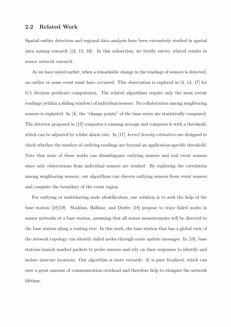
Figure 1: An N ∗ neighborhood of sensor Si and N neighborhoods of sensors inside N ∗(Si).

Each N neighborhood is used to compute di, while the N ∗(Si) is used to compare the di’s.

denote the measurement at Si1, Si2, · · ·, Sik, respectively. A comparison between xi and

{x(i)1 , x

(i)2 , · · · , x(i)

k } could be done by checking the difference between xi and the “center” of

{x(i)1 , x

(i)2 , · · · , x(i)

k }. Clearly, such a difference is

di = xi −medi, (1)

where medi denotes the median of the set {x(i)1 , x

(i)2 , · · · , x(i)

k }. We note that medi in Eq. (1)

should not be replaced by the mean (x(i)1 + x

(i)2 + · · ·+ x

(i)k )/k of the set {x(i)

1 , x(i)2 , · · · , x(i)

k }.

This is because the sample mean can not represent the “center” of a sample well when some

values of the sample are extreme. However, median is a robust estimator of the “center” of

a sample. If di is large or large but negative, then it is very likely that Si is an outlier. Now

we start to quantify the degree of extremeness of di. To do this, we need the differences d

that are associated with sensors near Si and computed via Eq (1).

Consider another bounded closed set N ∗(Si) ⊂ R2 that contains Si and additional n− 1

sensors. This set N ∗(Si) also represents a neighborhood of Si. Among many choices of

N ∗(Si), one could select N ∗(Si) = N (Si). We denote the n sensors in N ∗(Si) by S1, · · ·, Si,

· · ·, Sn. See Fig. 1 for an illustration of N and N ∗. According to Eq. (1) sensors in N ∗(Si)

yield d1, · · ·, di, · · ·, dn. Now if di is extreme in D = {d1, · · · , di, · · · , dn}, Si will be treated

as an outlying sensor. The decision can be made vigorously using the following procedure.

Let µ̂ and σ̂ denote, respectively, the sample mean and sample standard deviation of the set

D, i.e.,

µ̂ =1

n

n∑i=1

di,

σ̂ =

√√√√ 1

n− 1

n∑i=1

(di − µ̂)2 .

Standardize the dataset D to obtain {y1, · · · , yi, · · · , yn}, where

y1 =d1 − µ̂

σ̂, · · · , yi =

di − µ̂

σ̂, · · · , yn =

dn − µ̂

σ̂. (2)

DECISION: If |yi| ≥ θ, treat Si as an outlying sensor. Here θ(> 1) is a preselected number.

We now start to justify the above decision making procedure under certain assumptions.

For this purpose, we first need some result of the median. Given N (Si), assume x(i)1 , x

(i)2 ,

· · ·, x(i)k form a sample from a population having a continuous distribution function F . Let

x(i)1 , x

(i)2 , · · ·, x

(i)k be rearranged in the order from least to greatest and let the ordered values

be x(i)(1), x

(i)(2), · · ·, x

(i)(k), where x

(i)(1) ≤ x

(i)(2) ≤ · · · ≤ x

(i)(k). Then Eq. (1) can be rewritten as

medi =

x(i)((k+1)/2) if k is odd

(x(i)(k/2) + x

(i)(k/2+1))/2 if k is even.

(3)

Assuming that the median of the distribution F is µ̃ and F (µ̃) = 0.5 has a unique solution,

we have the following

PROPOSITION: As k →∞, medi converges in probability to µ̃.

To prove, we first note the following special case of Theorem 9.6.5 in [21]: if kpk is a positive

integer such that pk = 0.5 + O(1/k), then as k → ∞, x(i)(kpk) converges in probability to µ̃.

For any real number a, let bac denote the largest integer less than or equal to a and let (a)

denote the difference a− bac. Then 0 ≤ (a) < 1. Set p1k = b0.5kc+1k

. Then

p1k =0.5k − (0.5k) + 1

k= 0.5 + O

(1

k

).

Let p2k = p1k−1/k. Then p2k = 0.5+O(1/k). Therefore, both x(i)(kp1k) and x

(i)(kp2k) converge in

probability to µ̃. Now the proposition follows from the observation that Eq. (3) is equivalent

to the following

medi =

x(i)(kp1k) if k is odd

(x(i)(kp1k) + x

(i)(kp2k))/2 if k is even.

The above property of median is established for a quite general class of F . Deeper results

of median are also available. For example, an asymptotic normal distribution of median can

be obtained under some general conditions [3].

Now consider the following simple scenario where i) readings of sensors in N ∗(Si), i.e.,

x1, · · ·, xn, are independent; ii) for each sensor Sj in N ∗(Si), the readings from the sensors in

N (Sj) form a sample of a normal distribution; iii) all the variances of the above mentioned

distributions are equal. Since the median is equal to the mean for any normal distribution,

it follows from the proposition and i)-iii) that as k becomes large, the sequence d1, · · ·,

dn form approximately a sample from a normal distribution with mean equal to 0. This

implies that as k is large, the sequence from standardization, i.e., y1, · · ·, yn, can be treated

as a sample from a standard normal population N(0, 1). When xi is particularly large or

small, compared with all the other x values, di will deviate markedly from all the other d

values. Consequently, |yi| will be large, which implies that yi will fall into the tail region

of the density of the standard normal population. However, if |yi| is large, the probability

of obtaining this observation yi is small and thus Si should be treated as outlying. When

θ = 2, the probability of observing a yi with |yi| ≥ 2 is about 5%.

3.2 Algorithm

Let C1 denote the set of sensors with |yi| ≥ θ. The set C1 is viewed as a set of sensors that are

claimed as outliers by the above procedure. The procedure in part 3.1 can be summarized

into the following algorithm.

ALGORITHM 1

1. Construct {N} and {N ∗}. For each sensor Si, perform the following steps.

2. Use {N (Si)} and Eq. (1) to compute di for sensor Si.

3. Use {N ∗(Si)} and Eq. (2) to compute yi for sensor Si.

4. If |yi| ≥ θ, where θ > 1 is predetermined, assign Si to C1. Otherwise, Si is treated as

a normal sensor.

Clearly, |C1|, the size of C1, depends on θ. Assuming the y values in Eq. (2) constitute a

sample of a standard normal distribution and the decisions are made independently, then if

θ is chosen so that the right tail area of the density of N(0, 1) is α, |C1| will be about α×N.

In practice, a sensor becomes outlying if i) data measurement or data collection makes

errors, or ii) some variability in the area surrounding the sensor has changed significantly, or

iii) the inherent function of the sensor is abnormal. In any of the three cases, readings from

outlying sensors do not reflect reality, so that they can be discarded before further analysis

on sensor data. However, outlying readings may contain valuable information related to

events and provide help in detecting the events. For this reason, issues concerning event

region detection will be addressed in the presence of data from outlying sensors.

4 Localized Event Boundary Detection

In this section, we describe our procedure for localized event region detection. To detect

an event region, it suffices to detect the sensor nodes near or on the boundary of the event.

We note that C1 may contain some normal sensors close to the event boundary. However,

Algorithm 1 usually does not effectively detect sensors close to the boundary of the event.

To illustrate this point, let us consider the simple situation where the event lies to one side

Event

S1

S i

l(=B( ))E

N *(S )i

N (S )1

Figure 2: Event E is the union of line l and the portion on the left hand side of l. Si is a

sensor located on B(E) and S1 is a sensor inside N ∗(Si). Both N ∗(Si) and N (S1) are closed

disks.

of a straight line. Suppose that readings of sensors in the event (region) E form a sample

from a normal distribution N(µ1, σ2) and sensor readings outside E form another sample

from N(µ2, σ2), where µ1 6= µ2, and σ is small compared to |µ1 − µ2|. {N} and {N ∗} are

constructed using closed disks. Consider a sensor Si that is close to the event boundary.

Below we will show that even under some quite favorable setting, such a sensor Si may not

be detected, i.e., assigned to C1 by Algorithm 1.

Assume that readings of sensors in a neighborhood of Si are within 2σ distance from the

means of their corresponding normal distributions. Take each N neighborhood of sensors in

N ∗(Si) to be sufficiently large. Due to uniformity of the deployment of sensors, calculation

based on Eq. (1) shows that each d follows N(0, σ2) approximately. For example, at sensor

S1 shown in Fig. 2, d1 follows approximately N(0, σ2). The reasoning is as follows. Let R1

denote the portion of N (S1) that lies on the right hand side of the event boundary, and R2

denote the remaining portion of N (S1). Then the area of R1 is larger than that of R2. Since

the sensors are uniformly distributed, the expected number of sensors in R1 is larger than

the expected number of sensors in R2. Then med1 will be obtained using the sensor readings

from R1. When σ is small compared to |µ1−µ2|, med1 is about µ2, so that d1, which is about

x1−µ2, follows approximately N(0, σ2). Furthermore, it is seen that y1,· · ·, yn from (2) form

B( )E

Event

P1

P2

A

B

S i

Figure 3: Illustration of random bisection. NN (Si) is the half disk containing P1, Si, P2,

and B.

approximately a sample of N(0, 1) where each member of the sample is within distance 2 of

the mean 0. Therefore, C1 from Algorithm 1 will not pick up this sensor Si if θ = 2.

So that sensors near and on B(E) can be detected efficiently, the procedure described

in Algorithm 1 should be modified. As motivated above, to detect a sensor Si close to the

boundary, we should select a special neighborhood NN (Si) such that di, compared with d

values from surrounding neighborhoods, is as extreme as possible. There are many options

in doing this. Here we describe two of them: random bisection and random trisection.

Random Bisection

Consider an Si from the set S − C1. Place a closed disk centered at Si. Randomly draw a

line through Si, dividing the disk into two halves. Calculate di in each half. Use NN (Si)

to denote the half disk yielding the largest |di|. For an illustration, consult Fig. 3. In the

figure, the line randomly chosen meets the boundary of the disk at points P1 and P2, and the

boundary of the event meets the boundary of the disk at points A and B. Due to uniformity

of sensor deployment, we see that |di| from the half disk containing P1, P2, B, and Si is the

largest, and hence this half will be used as NN (Si). After NN (Si) is found, the resulting

di will be used to replace the old di, keeping unchanged all the other d values from N ∗(Si).

Then perform the calculation in Eq. (2) and make a decision on Si. We note that for random

i

i i

i i i

A

B

P1

P3 P2

RS i

Event

B( )E

Figure 4: Illustration of random trisection. Sectors P1SiP2, P2SiP3, and P3SiP1 are numbered

as i, ii, and iii, respectively. Each sector contains an angle equal to 2π/3. NN (Si) is the

union of sectors i and iii.

bisection as well as random trisection introduced next, lines are drawn randomly to form

sectors simply due to the fact the location and shape of an event boundary are usually

unknown a priori.

Random Trisection

Consider a closed disk centered at Si ∈ S − C1. Randomly divide the disk into three sectors

with an equal area. Number the sectors as i, ii, and iii, as shown in Fig. 4. Form a union

using any two sectors and calculate di in each union (total =3). The union resulting in the

largest |di| is NN (Si). It is easy to see that in Fig. 4, NN (Si) is the union of sectors i

and iii. The di with the largest |di| will replace previous di, keeping all the other d values

unchanged from N ∗(Si), and subsequently a decision will be made on Si.

Event Boundary Determination

There are two options of the decision on Si, based on NN (Si). If |yi| < θ, Si would be

treated as a normal sensor. If |yi| ≥ θ, the sensor Si can be close to or far away from the

boundary B(E). Let C2 denote the set of all the sensors with |yi| ≥ θ. The set C2 is expected

to contain enough sensors close to the event boundary (See Fig. 5(c)). In general, C2 catches

0 5 10 15 20 25 300

5

10

15

20

25

30

0 5 10 15 20 25 300

5

10

15

20

25

30

(a) Data (b) C1

0 5 10 15 20 25 300

5

10

15

20

25

30

0 5 10 15 20 25 300

5

10

15

20

25

30

(c) C2 (d) C3

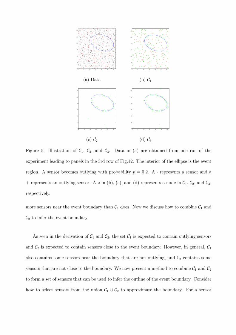
Figure 5: Illustration of C1, C2, and C3. Data in (a) are obtained from one run of the

experiment leading to panels in the 3rd row of Fig.12. The interior of the ellipse is the event

region. A sensor becomes outlying with probability p = 0.2. A · represents a sensor and a

+ represents an outlying sensor. A ◦ in (b), (c), and (d) represents a node in C1, C2, and C3,

respectively.

more sensors near the event boundary than C1 does. Now we discuss how to combine C1 and

C2 to infer the event boundary.

As seen in the derivation of C1 and C2, the set C1 is expected to contain outlying sensors

and C2 is expected to contain sensors close to the event boundary. However, in general, C1

also contains some sensors near the boundary that are not outlying, and C2 contains some

sensors that are not close to the boundary. We now present a method to combine C1 and C2

to form a set of sensors that can be used to infer the outline of the event boundary. Consider

how to select sensors from the union C1 ∪ C2 to approximate the boundary. For a sensor

Si ∈ C1 ∪ C2, draw a closed disk D(Si; c) with radius c centered at Si. The expected number

of sensors falling into the disk is m = πc2Nb2

. Since sensor readings are usually correlated

and C2 mainly contributes to the set of sensors near the event boundary, Si is expected to

be close to the boundary if D(Si; c) contains at least one sensor from C2 that is different

from Si. For any positive integer m, let C3(m) denote the subset of C1 ∪ C2 such that for

each Si ∈ C3(m), the disk D(Si;√

mb2

πN) contains at least one sensor from C2 that is different

from Si. The set C3(m) will serve as a set of sensors used to infer the event boundary (See

Fig. 5(d)). For convenience, sometimes we will write C3 for C3(m).

Now we summarize the above procedure of finding C2 and C3 into the following algorithm.

ALGORITHM 2

1. Construct {N} and {N ∗}. Apply Algorithm 1 to produce the set C1 (θ = θ1).

2. For each sensor Si ∈ S − C1, perform the following steps. Obtain NN (Si) and update

di from step 1 to the new di from NN (Si), keeping unchanged all the other d values

from N ∗(Si) obtained in step 1. Use Eq. (2) to recompute yi. If |yi| ≥ θ, assign Si to

set C2 (θ = θ2); otherwise, treat Si as a normal sensor.

3. Obtain C3(m), where m is a predetermined positive integer.

We stress on the following points on the use of the algorithm. First, the updated di in

step 2 is only needed when making a decision on sensor Si. Once such a decision is made,

this new di will have to be changed back to the original one obtained in step 1. Second,

assuming the y values in Eq. (2) constitute a sample of a standard normal distribution and

the decisions are made independently, then if θ1 and θ2 are such that the right tail areas of

the density of N(0, 1) are α1 and α2, respectively, the size of C2 is about (1− α1)× α2 ×N .

Third, unlike Algorithm 1, which utilizes the topological information of sensor locations to

find C1, Algorithm 2 uses the geographical information of locations to locate C2 and C3.

To conclude this section, we make the following note on the computational complexity

of Algorithms 1 and 2. Assume N ∗(Si) = N (Si) for each sensor Si, which is usually the

case in a densely deployed sensor network. Let ρ denote the average number of sensors in a

typical neighborhood N , which is also the average number of neighboring sensors in the given

network. Then it can be easily shown that both Algorithms 1 and 2 have a computational

complexity of O(ρ logρ). Since each sensor broadcasts a constant number of messages, the

message complexity of both algorithms is O(ρ).

5 Performance Evaluation

Evaluation of the proposed algorithms include two tasks: evaluating C1 and evaluating C3.

In this section, we first define metrics to evaluate C1. Then we examine what type of sensors

could be detected as being in C2 by Algorithm 2. The finding is then used to define metrics

to evaluate the performance of C3.

5.1 Evaluation of C1

To evaluate the performance of C1, we compute the detection accuracy a(C1), defined to be

the ratio of the number of outlying sensors detected to the total number of outlying sensors,

and the false alarm rate e(C1), defined to be the ratio of the number of normal sensors that

are claimed as outlying to the total number of normal sensors. Let O denote the set of

outliers in the field, then

a(C1) =|C1 ∩ O||O| , e(C1) =

|C1 −O|N − |O| . (4)

If a(C1) is high and e(C1) is low, Algorithm 1 has a good performance.

P1

P2P3

A

B

S i

ii

iiii

Event

B( )E

r

R

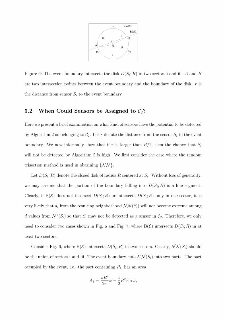
Figure 6: The event boundary intersects the disk D(Si; R) in two sectors i and iii. A and B

are two intersection points between the event boundary and the boundary of the disk. r is

the distance from sensor Si to the event boundary.

5.2 When Could Sensors be Assigned to C2?

Here we present a brief examination on what kind of sensors have the potential to be detected

by Algorithm 2 as belonging to C2. Let r denote the distance from the sensor Si to the event

boundary. We now informally show that if r is larger than R/2, then the chance that Si

will not be detected by Algorithm 2 is high. We first consider the case where the random

trisection method is used in obtaining {NN}.

Let D(Si; R) denote the closed disk of radius R centered at Si. Without loss of generality,

we may assume that the portion of the boundary falling into D(Si; R) is a line segment.

Clearly, if B(E) does not intersect D(Si; R) or intersects D(Si; R) only in one sector, it is

very likely that di from the resulting neighborhood NN (Si) will not become extreme among

d values from N ∗(Si) so that Si may not be detected as a sensor in C2. Therefore, we only

need to consider two cases shown in Fig. 6 and Fig. 7, where B(E) intersects D(Si; R) in at

least two sectors.

Consider Fig. 6, where B(E) intersects D(Si; R) in two sectors. Clearly, NN (Si) should

be the union of sectors i and iii. The event boundary cuts NN (Si) into two parts. The part

occupied by the event, i.e., the part containing P1, has an area

A1 =πR2

2πω − 1

2R2 sin ω,

B

A

P3

P1

P2

S i R

iiii

ii

r

Event

B( )E

Figure 7: The event boundary intersects the disk D(Si; R) in three sectors i, ii, and iii. A

and B are two intersection points between the event boundary and the boundary of the disk.

r is the distance from sensor Si to the event boundary.

where ω ∈ (0, π] is the value of ∠ASiB. And consequently, the area of the other part is

A2 =πR2

2π(4π

3)− A1.

So that di from NN (Si) becomes extreme, we require A1 ≥ A2, which implies

2(πR2

2πω − 1

2R2 sin ω) ≥ πR2

2π(4π

3).

Simplification leads to ω − 2π3≥ sinω. We see that ω ≥ 2π

3, since sin ω ≥ 0. Then

r = R cosω

2≤ R cos

(1

2

2π

3

)=

R

2.

Now consider Fig. 7, where B(E) intersects D(Si; R) in all three sectors. Let ω ∈ (0, π]

be the value of ∠ASiB. Then ω ≥ 2π/3. So r = R cos ω2≤ R

2. Summarizing the above shows

that r < R2.

Similarly, when the random bisection method is used in obtaining {NN}, we can also

show that r < R2.

Due to the above property of R, we call R/2 the tolerance radius.

5.3 Evaluation of C3

Here we first describe a quantity to judge how well C3 can be used to fit the boundary. Then

we present a quantity to examine how many sensors that are “far away” are included in C3.

We begin with the following definition.

DEFINITION: For a positive number r, let BA(E ; r) denote the set of all points in R2 such

that the distance of each point to the boundary B(E) is at most r. The degree of fitting of

C3 is defined to be

a(C3, r) =|BA(E ; r) ∩ C3||BA(E ; r) ∩ S| . (5)

Intuitively, BA(E ; r) is a strip with width 2r centered around the event boundary. The

quantity a(C3, r) is expected to provide valuable information on whether or not the detection

algorithm performs well in detecting the boundary of the event. The reasoning is as follows.

Suppose BA(E ; r) is such that all the sensors in BA(E ; r) provide a good outline of the

boundary B(E). If a(C3, r) is large, say, above 90%, then all the sensors in BA(E ; r) that are

detected by an event detection algorithm are also expected to provide a good outline of the

boundary of the event.

The value of r plays an important role in interpreting BA(E ; r) and a(C3, r). If r is large,

say, above R/2, then the above Section 5.2 shows that many sensors within BA(E ; r) will

not be detected so that a(C3, r) can be very low. On the other hand, if r is very small,

BA(E ; r) may become a strip containing few sensors so that BA(E ; r) does not present a

good description of the boundary B(E). A natural question is then: how can one choose

an appropriate r such that BA(E ; r) provides a good outline of the boundary and a(C3, r) is

informative?

To get an answer, we first note that if these N sensors are placed into the field using

the standard grid method, then a typical grid is a square with width equal to b/√

N . Given

BA(E ; r), randomly draw a square Q “inside” BA(E ; r) such that i) its width is 2r; ii) two

sides of the square are “perpendicular” to the boundary B(E). See Fig. 8 for an example of

Q.

Set 2r = c× b√N

, where c is to be determined. That is, the width of the fitted square Q

Q2r

B( ; )E r

B( )E

Figure 8: An illustration of the square Q fitted into the boundary area.

equals c times the width of a typical grid square. Clearly, the expected number of sensors

caught by Q is

N ×( area of Q

area of sensor field

)=

N × (c× b√N

)2

b2= c2.

For BA(E ; r) to provide a good outline of the boundary, intuitively, we could choose r such

that c2, the expected number of sensors inside Q, equals 1. When c2 = 1, r has the following

value

r1 =1

2(

b√N

). (6)

Note that r1 equals half width of a typical grid.

We now turn to examining how many sensors not close to the boundary are contained in

C3. Motivated by Section 5.2, we only check those sensors whose distances to the boundary

are at least R/2. Let A(E ; R) denote the set of all points in R2 such that the distance of

each point to the boundary B(E) is at least R/2. Define the false detection rate of C3 to be

the following quantity

e(C3, R) =|A(E ; R) ∩ C3||A(E ; R) ∩ S| . (7)

If e(C3, R) is small, sensors far away from the event boundary are not likely to be contained

in C3.

6 Simulation

In this section, we describe our simulation set-up, discuss the issue of determination of

threshold values, and report our experimental results.

6.1 Simulation Set-Up

We use MATLAB to perform all simulations. All the sensor nodes are uniformly distributed

in a 64 × 64 square region. The number of nodes is 4096. Without loss of generality, we

assume the square region resides in the first quadrant such that the lower-left corner and the

origin are co-located. Sensor coordinates are defined accordingly. Normal sensor readings

are drawn from N(µ1, σ21) while event sensor readings are drawn from N(µ2, σ

22). In the

simulation we choose µ1 = 10, µ2 = 30, σ1 = σ2 = 1. Note that these means and variances

can be picked arbitrarily as long as |µ1 − µ2| is large enough compared with σ1 and σ2. We

choose σ1 = σ2 = 1 because they represent the system calibration error which should be

small for a sensor that is not outlying.

In all the simulation scenarios, we choose N = N ∗, and N (Si) contains all one-hop

neighbors of Si. Construction of NN (Si) is based on N (Si). Increasing the size of N

requires increasing either the transmission range, to enlarge the one-hop neighbor set, or the

hop count. We note that multihop neighborhood information implies high communication

overhead. Since our simulation focuses on the evaluation of the proposed algorithms, we

choose to increase the transmission range and thus N always contains one-hop neighbors.

We call the average number of sensors in N the density of the sensor network.

To simulate ALGORITHM 1 for outlying sensor detection, no event is generated in the

network region. All outlying values are drawn from N(30, 1). In the simulation of event

boundary detection, a sensor in the event region gets a value from N(10, 1) with probability

p and a value from N(30, 1) with probability 1 − p. A sensor out of the event region gets

a value from N(30, 1) with probability p and a value from N(10, 1) with probability 1 − p.

These settings are selected to make readings from an event region and readings outside

the region largely interfere with each other. Though various event regions with different

boundary shapes can be considered, in this paper we focus on two typical cases: the event

regions with ellipses or straight lines as the boundaries. Straight lines are selected because

when the event region is large, the view of a sensor near the boundary is approximated

by a line segment in most cases. An ellipse represents a curly boundary. Our simulation

produces similar results for event regions with other boundary shapes. The event regions are

generated as follows. For a linear boundary, a line y = kx + b is computed, where k = tanγ

is the slope, with γ drawn randomly from (0, π2), and b is the intercept, drawn randomly

from (−16, 16). The area below the line is the event region. For a curly boundary, the event

region is bounded by an ellipse that can be represented by E(a, b, x0, y0, ν) = 0 [6]. Here 2a

and 2b are the lengths of the major and minor axes of the ellipse, with a, b drawn randomly

from [4,16]. (x0, y0) is the center of the ellipse, where x0 and y0 are randomly chosen from

[a, 64 − a]. ν, the angle between the major axis of the ellipse and the x-axis, is a random

number between 0 and π.

Note that both algorithms 1 and 2 need thresholds θ1 and θ2 to compute C1 and C2.

Determination of these values is discussed in the next subsection.

6.2 Determination of Thresholds

One possibility of obtaining the threshold values [9] is to estimate them according to p,

the probability that a sensor becomes outlying. For example, from the theory of normal

distributions, the ideal relationship between θ1 and p, under the strict assumptions stated

after ALGORITHM 1, may be seen partially in Table 1. However, due to practical violations

of the assumptions, the actual relationship might deviate significantly from the one listed in

p 0.26% 5% 10% 15% 20% 25%

θ1 3.00 1.96 1.65 1.44 1.28 1.15

Table 1: Relationship between θ1 and p when y’s are iid (Identical Independent Distribution)

from N(0, 1).

the table. Therefore, to obtain more accurate detection results, one needs some alternative

methods to estimate the threshold settings. For convenience, we simply choose θ2 = θ1 = θ

in this paper, because both algorithms 1 and 2 follow the same procedure except that they

utilize different neighborhoods to compute d value. This means that once we have an estimate

for θ1, the same estimate will also be used for θ2. In this section, we propose to determine

θ1 using an adaptive threshold determination scheme through the ROC (receiver operating

characteristic) curve analysis [10].

Here is the idea of this scheme. Periodically the base station queries a subregion, where no

event occurs, to obtain a training dataset and then executes the algorithm for outlying sensor

detection based on different threshold settings. We note that the utilization of such training

data is practical in the sensor networks [2, 8]. Each time, the false alarm rates and detection

accuracies based on one query are used to construct an ROC curve, where the abscissa

represents the false alarm rate, and the ordinate denotes the detection accuracy. This curve

outlines the relationship between the accuracy and the false alarm rate when varying the

threshold values of θ. The well-known fact is that an improvement in the detection accuracy

is usually accompanied by an increase in the false alarm rate. A common practical choice

of θ is obtained from the knee point on the curve where the detection accuracy increases

limitedly while the false alarm rate exhibits a large boost. Base station will then broadcast

the settings of the thresholds to the whole network.

In our simulation studies, we only consider the following six threshold settings: 3, 1.96,

1.65, 1.44, 1.28, 1.15, as shown in Table 1. For each query, the training data set contains

196 nodes, i.e., about 5% of the entire network. In the light of the ratio of the increase

in detection accuracy to the increase in false alarm rate, one of these six settings will be

selected as the optimal setting that corresponds to the knee point. Details are provided as

follows.

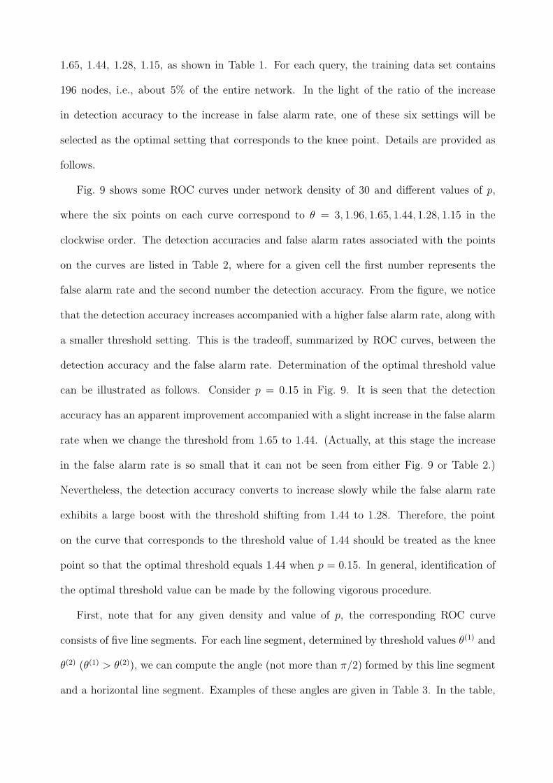
Fig. 9 shows some ROC curves under network density of 30 and different values of p,

where the six points on each curve correspond to θ = 3, 1.96, 1.65, 1.44, 1.28, 1.15 in the

clockwise order. The detection accuracies and false alarm rates associated with the points

on the curves are listed in Table 2, where for a given cell the first number represents the

false alarm rate and the second number the detection accuracy. From the figure, we notice

that the detection accuracy increases accompanied with a higher false alarm rate, along with

a smaller threshold setting. This is the tradeoff, summarized by ROC curves, between the

detection accuracy and the false alarm rate. Determination of the optimal threshold value

can be illustrated as follows. Consider p = 0.15 in Fig. 9. It is seen that the detection

accuracy has an apparent improvement accompanied with a slight increase in the false alarm

rate when we change the threshold from 1.65 to 1.44. (Actually, at this stage the increase

in the false alarm rate is so small that it can not be seen from either Fig. 9 or Table 2.)

Nevertheless, the detection accuracy converts to increase slowly while the false alarm rate

exhibits a large boost with the threshold shifting from 1.44 to 1.28. Therefore, the point

on the curve that corresponds to the threshold value of 1.44 should be treated as the knee

point so that the optimal threshold equals 1.44 when p = 0.15. In general, identification of

the optimal threshold value can be made by the following vigorous procedure.

First, note that for any given density and value of p, the corresponding ROC curve

consists of five line segments. For each line segment, determined by threshold values θ(1) and

θ(2) (θ(1) > θ(2)), we can compute the angle (not more than π/2) formed by this line segment

and a horizontal line segment. Examples of these angles are given in Table 3. In the table,

0 0.02 0.04 0.06 0.080

0.2

0.4

0.6

0.8

1

False alarm rate

Det

ectio

n ac

cura

cy

p=0.05p=0.10p=0.15p=0.20

Figure 9: Examples of ROC curves for density = 30 and different values of p.

the five components under a value of p are angles corresponding to θ1 = 3.00, 1.96, 1.65, 1.44,

and 1.28, respectively. Clearly, the angle derived from a line segment depends on the ratio

of the increase in detection accuracy to the increase in false alarm rate. Table 3 shows

that as θ(1) decreases, the angle decreases. As the angle becomes smaller, the line segment

becomes less steep. Our experience shows that the following is an efficient way to choose

the optimal threshold value: if there exists at least one pair (θ(1), θ(2)) such that the angle

from the corresponding line segment is less than 1.5(i.e., 86◦), the largest value of such θ(1)

is selected as the optimal setting of the threshold; otherwise, 1.15 (the smallest among the

six preselected values of the threshold setting) is chosen as the optimal setting. Reconsider

the case with density =30 and p = 0.15. It follows from Table 3 that only angles from the

line segments corresponding to (θ(1), θ(2)) = (1.44, 1.28) and (1.28, 1.15) are less than 1.5.

Then the largest θ(1) value such that the angle is less than 1.5 is 1.44. Therefore, 1.44 is the

optimal threshold value. Optimal threshold values, derived from Table 3, are provided in

Table 4. We see that the optimal threshold setting is smaller when there are more outlying

sensors in the network, i.e., p is larger.

θ p = 0.05 p = 0.10 p = 0.15 p = 0.20

3 0.0000 0.0000 0.0000 0.0000

0.4444 0.1875 0.0000 0.0000

1.96 0.0053 0.0000 0.0000 0.0000

1.0000 0.6250 0.5000 0.2857

1.65 0.0107 0.0000 0.0000 0.0000

1.0000 0.8750 0.7500 0.5000

1.44 0.0214 0.0000 0.0000 0.0000

1.0000 0.8750 0.8571 0.5476

1.28 0.0374 0.0111 0.0060 0.0130

1.0000 1.0000 0.8929 0.7381

1.15 0.0642 0.0222 0.0119 0.0455

1.0000 1.0000 0.9286 0.8571

Table 2: False alarm rates and detection accuracies associated with the points indicated on

the ROC curves in Fig. 9.

p = 0.05 p = 0.10 p = 0.15 p = 0.20

1.5612 1.5708 1.5708 1.5708

0 1.5708 1.5708 1.5708

0 1.5708 1.5708 1.5708

0 1.4821 1.4056 1.5027

0 0 1.4056 1.3045

Table 3: Angles of line segments of ROC curves in Fig. 9.

p = 0.05 p = 0.10 p = 0.15 p = 0.20

θ 1.96 1.44 1.44 1.28

Table 4: Optimal threshold values derived from Table 3.

6.3 Simulation Results

In this subsection, we report our simulation results, each representing an averaged summary

over 100 runs. More specifically, for each run of computation, the sensor field with or without

an event region is generated using the procedure in Subsection 6.1, the optimal threshold

value is determined using the method described in Subsection 6.2, and then Algorithm 1

or Algorithm 2 is applied to obtain the values of the performance metrics. The averaged

values of the performance metrics over 100 runs are reported as our simulation findings. The

performance metrics include the detection accuracy and false alarm rate for outlying sensor

detection, as defined by Eq. (4) in Subsection 5.1 for the evaluation of C1, and the degree

of fitting and false detection rate for event boundary detection, as defined by Eq. (5) and

(7) in Subsection 5.3 for the evaluation of C3. Recall that two sets, C1 and C3, contain the

detected outlying sensors and boundary sensors respectively.

We note that based on the detection accuracy and false alarm rate, one usually has a

good idea on whether or not our outlying sensor detection algorithm works well in practice.

However, the use of information on the degree of fitting and false detection rate is somewhat

subjective. Sometimes, our algorithm yields a clear outline of the event boundary, but the

degree of fitting can be low and false detection rate can be high. In this paper, we do not

make any effort in trying to determine what values of the degree of fitting and false detection

rate could indicate that the event boundary has been successfully located. The related issue

will be addressed in our future work.

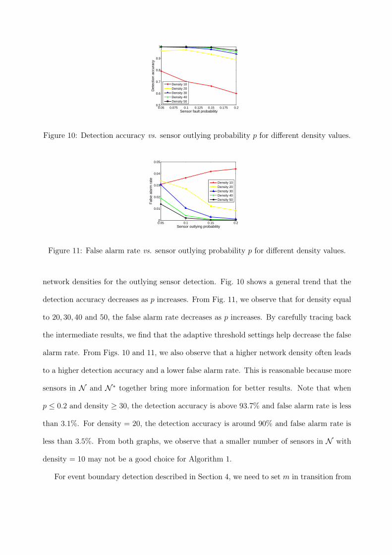
Figs. 10 and 11 plot the detection accuracy and false alarm rate vs. p, under different

0.05 0.075 0.1 0.125 0.15 0.175 0.20.5

0.6

0.7

0.8

0.9

1

Sensor fault probability

Det

ectio

n ac

cura

cy

Density 10Density 20Density 30Density 40Density 50

Figure 10: Detection accuracy vs. sensor outlying probability p for different density values.

0.05 0.1 0.15 0.20

0.01

0.02

0.03

0.04

0.05

Sensor outlying probability

Fal

se a

larm

rat

e

Density 10Density 20Density 30Density 40Density 50

Figure 11: False alarm rate vs. sensor outlying probability p for different density values.

network densities for the outlying sensor detection. Fig. 10 shows a general trend that the

detection accuracy decreases as p increases. From Fig. 11, we observe that for density equal

to 20, 30, 40 and 50, the false alarm rate decreases as p increases. By carefully tracing back

the intermediate results, we find that the adaptive threshold settings help decrease the false

alarm rate. From Figs. 10 and 11, we also observe that a higher network density often leads

to a higher detection accuracy and a lower false alarm rate. This is reasonable because more

sensors in N and N ∗ together bring more information for better results. Note that when

p ≤ 0.2 and density ≥ 30, the detection accuracy is above 93.7% and false alarm rate is less

than 3.1%. For density = 20, the detection accuracy is around 90% and false alarm rate is

less than 3.5%. From both graphs, we observe that a smaller number of sensors in N with

density = 10 may not be a good choice for Algorithm 1.

For event boundary detection described in Section 4, we need to set m in transition from

C1 and C2 to C3. Through simulation studies we observe that a larger m usually results in a

higher degree of fitting and a higher false detection rate, when the network density and p are

fixed. For convenience, we fix m = 4 in the following, since this setting in general achieves

a good degree of fitting and a low false detection rate. Plots of the experimental results are

shown in Fig. 12 for various scenarios.

The main observations from these plots are summarized in the following. a) For a fixed

density, as p increases, the degree of fitting tends to decrease and the false detection rate

tends to increase. The main reason for this is that for a larger p, more outlying sensors

interfere with boundary nodes. b) For a fixed sensor outlying probability, as density increases,

the degree of fitting tends to become larger and the false detection rate tends to become

smaller. This is due to the fact that with a higher density, more information is available

for the detection algorithms. c) For a given shape (line or ellipse) of the event boundary,

the random trisection method outperforms the random bisection method. This is because

random trisection induces a larger NN so that more information is utilized in the detection

process.

From Fig. 12, we see that the degree of fitting is low for the cases where density equals

10. Note that a low degree of fitting does not mean that the boundary can not be detected.

Instead it means that more sensors close to the boundary escape the detection. For example,

Fig. 5(d) indicates a case where the degree of fitting is as low as 53% for p = 0.2. However,

for such a low value of the degree of fitting, the elliptical boundary is still clearly identified.

(In this scenario, the outlying sensor detection accuracy is 92%.)

We have also conducted simulations when input data are binary decision predicates and

obtained results close to those reported in Fig. 12. This indicates that our algorithms are

applicable to both 0/1 decision predicates and numeric sensor readings.

7 Conclusions and Future Works

In this paper, we present localized algorithms for the identification of outlying sensors and

event boundary in sensor networks. We also propose a scheme to adaptively adjust the

thresholds in the base station. Simulation results indicate that these algorithms can clearly

detect the event boundary and can identify outlying sensors with a high accuracy and a low

false alarm rate when as many as 20% of the outlying readings exist.

We believe that our ideas in detecting outlying sensors and event boundaries can be

extended to multi-modality sensor networks, and the data aggregation can be done along

both temporal and spatial dimensions for decreasing the false alarm rate in outlying sensor

detection and the false detection rate for boundary detection. Thus we propose to explore

along these directions in the future. We will further study the minimum density requirement

for an expected detection accuracy of our proposed algorithms, which can be used as a

guideline for the selection of the neighborhood N and/or N ∗ in real network scenarios.

Furthermore, we intend to study other techniques for thresholds (both θ1 and θ2) compu-

tation. For example, θ values may be determined based on the minimization of a cost-based

system. We will conduct more simulations for the case of θ1 6= θ2 to study the performance

of the proposed algorithms. We also plan to study the robust estimates for the population

standard deviation. These estimates will replace the corresponding estimates, such as σ̂ in

equation (2), in the present description of our algorithms. Robust estimates are less influ-

enced by the values of outlying sensors. A potential benefit of the use of robust estimates of

population standard deviation is that we could use the percentiles of the standard normal

distribution or χ21 to make decisions instead of the thresholds.

References

[1] V. Barnet and T. Lewis, Outliers in Statistical Data, John Wiley and Sons, Inc., 1994.

[2] R. Brooks, P. Ramanathan and A. Sayeed, Distributed Target Classification and Track-

ing in Sensor Networks, Proc. IEEE, pp. 1163-1171, Vol. 91, No. 8, August 2003.

[3] D. Chen and X. Cheng, An Asymptotic Analysis of Some Expert Fusion Methods,

Pattern Recognition Letters, 22, 901-904, 2001.

[4] D. Chen, X. Cheng, and M. Ding, Localized Event Detection in Sensor Networks,

manuscript, 2004.

[5] X. Cheng, A. Thaeler, G. Xue, and D. Chen, TPS: A Time-Based Positioning Scheme

for Outdoor Sensor Networks, IEEE INFOCOM, HongKong China, March 2004.

[6] K.K. Chintalapudi and R. Govindan, Localized Edge Detection in Sensor Fields, IEEE

Ad Hoc Networks Journal, pp. 59-70, 2003.

[7] T. Clouqueur, K.K. Saluja, and P. Ramanathan, Fault Tolerance in Collaborative Sensor

Networks for Target Detection, IEEE Transactions on Computers, pp. 320-333, Vol. 53,

No. 3, March 2004.

[8] Amol Deshpande, Carlos Guestrin, Samuel Madden, Joseph Hellerstein, and Wei Hong,

Model Driven Data Acquisition in Sensor Networks, 30th International Conference on

Very Large Data Bases , VLDB 2004, Toronto, Canada.

[9] M. Ding, D. Chen, K. Xing, and X. Cheng, Localized Fault-Tolerant Event Boundary

Detection in Sensor Networks, IEEE INFOCOM, March 2005, Miami Florida.

[10] Richard O. Duda, Peter E. Hart, and David G. Stork, Pattern Classification, Wiley-

Interscience, New York, 2000.

[11] B. Krishnamachari and S. Iyengar, Distributed Bayesian Algorithms for Fault-Tolerant

Event Region Detection in Wireless Sensor Networks, IEEE Transactions on Computers,

Vol. 53, No. 3, pp. 241-250, March 2004.

[12] K. Krivoruchko, C. Gotway, and A. Zhigimont, Statistical Tools for Regional Data

Analysis Using GIS, GIS’03, pp. 41-48, New Orleans, LA, November 2003.

[13] D. Li, K.D. Wong, Y.H. Hu, and A.M. Sayeed, Detection, Classification, and Tracking

of Targets, IEEE Signal Processing Magazine, Vol. 19, pp. 17-29, March 2002.

[14] F. Liu, X. Cheng, D. Hua, and D. Chen, Range-Difference Based Location Discovery

for Sensor Networks with Short Range Beacons, to appear in International Journal on

Ad Hoc and Ubiquitous Computing, 2007.

[15] C.T. Lu, D. Chen, and Y. Kou, Detecting Spatial Outliers with Multiple Attributes,

Proceedings of 15th International Conference on Tools with Artificial Intelligence pp.

122-128, November 2003.

[16] C.T. Lu, D. Chen, and Y. Kou, Algorithms for Spatial Outlier Detection, Proceedings

of 3rd IEEE International Conference on Data Mining, pp. 597-600, November 2003.

[17] T. Palpanas, D. Papadopoulos, V. Kalogeraki, and D. Gunopulos, Distributed Deviation

Detection in Sensor Networks, SIGMOD Record, 32(4), pp. 77-82, December 2003.

[18] J. Staddon, D. Balfanz, and G. Durfee, Efficient Tracing of Failed Nodes in Sensor

Networks, ACM WSNA’02, pp. 122-130, Atlanta, GA, September 2002.

[19] S. Tanachaiwiwat, P. Dave, R. Bhindwale, A. Helmy, Location-centric Isolation of Mis-

behavior and Trust Routing in Energy-constrained Sensor Networks, the Workshop on

Energy-Efficient Wireless Communications and Networks (EWCN 2004), Phoenix, Ari-

zona, April 14-17, 2004.

[20] A. Thaeler, M. Ding, X. Cheng, and D. Chen, iTPS: An Improved Location Discov-

ery Scheme for Sensor Networks with Long Range Beacons, Journal of Parallel and

Distributed Computing, 65(2), pp.98-106, Feburary 2005.

[21] S. S. Wilks, Mathematical Statistics, Wiley, New York, 1962.

0 0.05 0.1 0.15 0.20.1

0.125

0.15

0.175

0.2

0.225

0.25

0.275

0.3

Sensor outlying probability

Deg

ree

of fi

tting

Trisection for ellipseBisection for ellipseTrisection for straight lineBisection for sraight line

0 0.05 0.1 0.15 0.20

0.005

0.01

0.015

0.02

0.025

0.03

Sensor outlying probability

Fal

se d

etec

tion

rate

Trisection for ellipseBisection for ellipseTrisection for straight lineBisection for straight line

0 0.05 0.1 0.15 0.20.3

0.35

0.4

0.45

0.5

0.55

0.6

0.65

0.7

Sensor outlying probability

Deg

ree

of fi

tting

Trisection for ellipseBisection for ellipseTrisection for straight lineBisection for sraight line

0 0.05 0.1 0.15 0.20

0.005

0.01

0.015

0.02

0.025

Sensor outlying probabilityF

alse

det

ectio

n ra

te

Trisection for ellipseBisection for ellipseTrisection for straight lineBisection for straight line

0 0.05 0.1 0.15 0.20.4

0.5

0.6

0.7

0.8

0.9

Sensor outlying probability

Deg

ree

of fi

tting

Trisection for ellipseBisection for ellipseTrisection for straight lineBisection for sraight line

0 0.05 0.1 0.15 0.20

0.002

0.004

0.006

0.008

0.01

Sensor outlying probability

Fal

se d

etec

tion

rate

Trisection for ellipseBisection for ellipseTrisection for straight lineBisection for straight line

0 0.05 0.1 0.15 0.20.5

0.6

0.7

0.8

0.9

1

Sensor outlying probability

Deg

ree

of fi

tting

Trisection for ellipseBisection for ellipseTrisection for straight lineBisection for sraight line

0 0.05 0.1 0.15 0.20

1

2

3

4

5

6x 10

−3

Sensor outlying probability

Fal

se d

etec

tion

rate

Trisection for ellipseBisection for ellipseTrisection for straight lineBisection for straight line

0 0.05 0.1 0.15 0.20.5

0.6

0.7

0.8

0.9

1

Sensor outlying probability

Deg

ree

of fi

tting

Trisection for ellipseBisection for ellipseTrisection for straight lineBisection for sraight line

0 0.05 0.1 0.15 0.20

0.5

1

1.5

2

2.5

3

3.5

4x 10

−3

Sensor outlying probability

Fal

se d

etec

tion

rate

Trisection for ellipseBisection for ellipseTrisection for straight lineBisection for straight line

Figure 12: Performance of the event boundary detection algorithm under different values of

sensor outlying probability p and network density. The 1st, 2nd, 3rd, 4th, and 5th row has

a density equal to 10, 20, 30, 40, and 50, respectively.