LOCAL REGULARIZATION METHODS FOR THE STABILIZATION...

LOCAL REGULARIZATION METHODS FOR THE STABILIZATION OF

LINEAR ILL-POSED EQUATIONS OF VOLTERRA TYPE

Patricia K. Lamm

Department of Mathematics, Michigan State University,E. Lansing, MI 48824-1027

E-mail: [email protected]

and

Thomas L. Scofield

Department of Mathematics and Statistics,Calvin College, Grand Rapids, MI 49546

E-mail: [email protected]

Inverse problems based on first-kind Volterra integral equations appear nat-urally in the study of many applications, from geophysical problems to the in-verse heat conduction problem. The ill-posedness of such problems means thata regularization technique is required, but classical regularization schemes likeTikhonov regularization destroy the causal nature of the underlying Volterraproblem and, in general, can produce oversmoothed results.

In this paper we investigate a class of local regularization methods in whichthe original (unstable) problem is approximated by a parameterized familyof well-posed, second–kind Volterra equations. Being Volterra, these approxi-mating second–kind equations retain the causality of the original problem andallow for quick sequential solution techniques. In addition, the regularizingmethod we develop is based on the use of a regularization parameter which isa function (rather than a single constant), allowing for more or less smooth-ing at localized points in the domain. We take this approach even further byadopting the flexibility of an additional penalty term (with variable penaltyfunction) and illustrate the sequential selection of the penalty function in anumerical example.

Key Words: Volterra first-kind problem, inverse problem, regularization, fast sequential algorithm

1. INTRODUCTION

We consider the following scalar Volterra first-kind integral problem. Given a suitable

function f(·) defined on [0, 1], find u(·) satisfying, for a.e. t ∈ [0, 1],

Au(t) = f(t), (1)

where A is the bounded linear operator on L2(0, 1) given by

Au(t) :=∫ t

0

k(t, s)u(s) ds, a.e. t ∈ [0, 1].

1

2 P. K. LAMM AND T. L. SCOFIELD

Problem (1) is an important one, having many applications. One is the inverse heat con-

duction problem (IHCP) or sideways heat equation [4] with convolution kernel k. In an

application from capillary viscometry, the integral equation takes the form of (1) with non-

convolution kernel k. In this case, f (the known function) is the apparent wall shear rate

(itself a measured quantity rather than the true wall shear rate) and the desired quantity,

the reciprocal of u(·), is the viscosity [29].

In the typical case that the range of A is not closed, it is well-known that problem (1) is

ill-posed, lacking continuous dependence on data f ∈ L2(0, 1). Thus, when using measured

or numerically-approximated data, one must resort to a regularization method to ensure

stability. There is a well-developed theory for classical methods such as Tikhonov regulariza-

tion (see, for example, [13]), but such methods are less than optimal for Volterra problems of

the form (1). For example, Tikhonov regularization replaces the original “causal” problem

with a full-domain one. By the causal nature of the original problem we mean that problem

(1) has the property that, for any t ∈ (0, 1], the solution u on the interval [0, t] is determined

only from values of f on that same interval; for this reason, sequential solution techniques

are optimal for causal problems. In contrast, to determine a solution via Tikhonov regu-

larization one must use data values from the interval [t, 1] (i.e., future data values), thus

destroying the causal nature of the original problem and leading to non-sequential solution

techniques.

Another difficulty arising in classical regularization techniques involves the use of a single

regularization parameter when a priori information indicates that a solution is rough in some

areas of the domain and smooth in others. In recent years a number of approaches have

been developed to handle this difficulty, among them the technique of bounded variation

regularization [1, 7, 11, 16, 17, 33], as well as the method of “regularization for curve

representations” [31]. Although effective, these approaches do not preserve the causal nature

of the original Volterra problem and, in addition, can require a reformulation of the linear

problem (or linear least-squares problem) into either a nondifferentiable or nonquadratic

optimization problem. In [30], a unified approach to regularization with nondifferentiable

functionals (including functionals of bounded variation type) is considered, with theoretical

treatment based on the concept of distributional approximation. The approach in [30] may

be adapted so that a localized type of regularization is possible, however the application of

this approach to Volterra equations has evidently not been studied.

Local regularization techniques form a different class of methods which have been the

focus of study in recent years. These methods retain both the linear and causal structure

of the original Volterra problem, allowing for solution via fast sequential methods, and rely

on differentiable optimization techniques for solution. And, because regularization occurs

in local regions only, sharp/fine structures of true solutions can often be recovered. The

development in [21, 22, 23, 25, 26] of such methods grew out of a desire to construct a the-

oretical framework for understanding a popular numerical method developed by J. V. Beck

VARIABLE REGULARIZATION METHODS 3

in the 1960’s for the IHCP. In this sequential method, Beck held solutions rigid for a short

time into the future (forming a locally regularized “prediction”), and then truncated the

prediction in order to improve accuracy (“correction”) before moving to the next step in

the sequence. Generalizations of Beck’s ideas also retain this “predictor-corrector” charac-

teristic when discretized. In general, the methods are easy to implement numerically and

provide fast results in almost real-time. (We note that mollifier methods for regularization

can also be considered local regularization methods; however such methods do not easily

apply to general equations of the form (1). See [24] and the references therein for a more

complete discussion.)

In what follows, we lay the groundwork for a general class of local regularization methods.

Our emphasis here is on a continuous method in which one may employ variable regulariza-

tion parameters to allow for local control of the stabilization process. This is an extension

of the continuous regularization method studied in [22] where a single (constant-valued)

local regularization parameter was employed. The change to functional regularization pa-

rameters requires a nontrivial redevelopment of the theory of [22]. In addition, it is worth

noting that convergence of a discrete version of the method presented below is studied in

[27], where it is shown that the resulting sequential regularization algorithm leads to con-

siderable savings in computational costs. Indeed the discrete local regularization algorithm

requires only O(N2) arithmetic operations while standard Tikhonov regularization requires

O(N3) operations (to highest order). In [27] we also propose and test a sequential algorithm

for the adaptive selection of one of the variable regularization parameters.

2. PRACTICAL IMPLEMENTATION OF A LOCAL REGULARIZATION

METHOD

Before discussing the continuous regularization method of interest in this paper, we mo-

tivate the work that follows by describing a practical implementation of our ideas. The

discussion in this section will focus on a discretization of the original equation (1), as well

as a discretization of the continuous regularization method to be analyzed in subsequent

sections.

2.1. Collocation-based discretization of the original Volterra problem

We first describe a simple collocation-based discretization of (1). We divide [0, 1] into

N subintervals [ti−1, ti], i = 1, . . . N , each of width ∆t = 1/N , and seek constants ci,

i = 1, . . . , N , so that the step function

u(t) =N∑

i=1

ciχi(t), t ∈ [0, 1], (2)


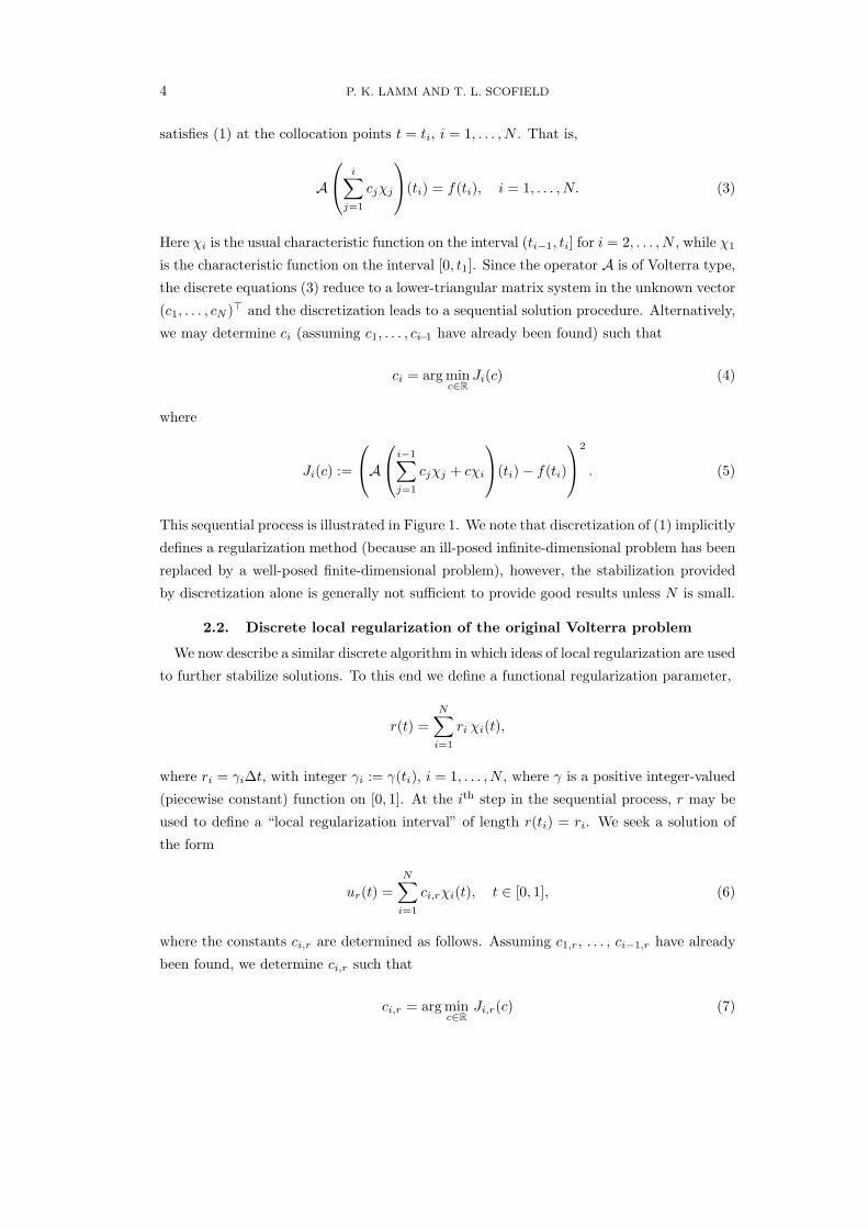
satisfies (1) at the collocation points t = ti, i = 1, . . . , N . That is,

A

i∑j=1

cjχj

(ti) = f(ti), i = 1, . . . , N. (3)

Here χi is the usual characteristic function on the interval (ti−1, ti] for i = 2, . . . , N , while χ1

is the characteristic function on the interval [0, t1]. Since the operator A is of Volterra type,

the discrete equations (3) reduce to a lower-triangular matrix system in the unknown vector

(c1, . . . , cN )> and the discretization leads to a sequential solution procedure. Alternatively,

we may determine ci (assuming c1, . . . , ci−1 have already been found) such that

ci = arg minc∈R

Ji(c) (4)

where

Ji(c) :=

Ai−1∑

j=1

cjχj + cχi

(ti)− f(ti)

2

. (5)

This sequential process is illustrated in Figure 1. We note that discretization of (1) implicitly

defines a regularization method (because an ill-posed infinite-dimensional problem has been

replaced by a well-posed finite-dimensional problem), however, the stabilization provided

by discretization alone is generally not sufficient to provide good results unless N is small.

2.2. Discrete local regularization of the original Volterra problem

We now describe a similar discrete algorithm in which ideas of local regularization are used

to further stabilize solutions. To this end we define a functional regularization parameter,

r(t) =N∑

i=1

ri χi(t),

where ri = γi∆t, with integer γi := γ(ti), i = 1, . . . , N , where γ is a positive integer-valued

(piecewise constant) function on [0, 1]. At the ith step in the sequential process, r may be

used to define a “local regularization interval” of length r(ti) = ri. We seek a solution of

the form

ur(t) =N∑

i=1

ci,rχi(t), t ∈ [0, 1], (6)

where the constants ci,r are determined as follows. Assuming c1,r, . . . , ci−1,r have already

been found, we determine ci,r such that

ci,r = arg minc∈R

Ji,r(c) (7)


where

Ji,r(c) :=γi∑

k=0

Ai−1∑

j=1

cjχj + ci+k∑`=i

χ`

(ti+k)− f(ti+k)

2

. (8)

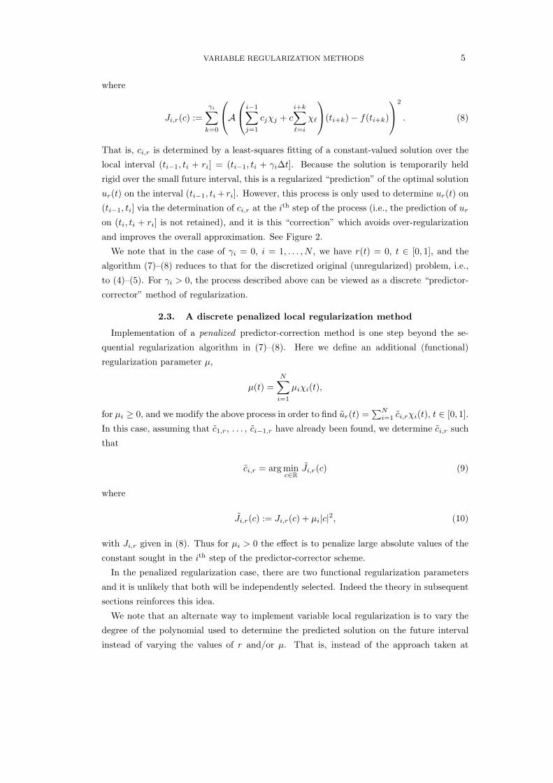
That is, ci,r is determined by a least-squares fitting of a constant-valued solution over the

local interval (ti−1, ti + ri] = (ti−1, ti + γi∆t]. Because the solution is temporarily held

rigid over the small future interval, this is a regularized “prediction” of the optimal solution

ur(t) on the interval (ti−1, ti + ri]. However, this process is only used to determine ur(t) on

(ti−1, ti] via the determination of ci,r at the ith step of the process (i.e., the prediction of ur

on (ti, ti + ri] is not retained), and it is this “correction” which avoids over-regularization

and improves the overall approximation. See Figure 2.

We note that in the case of γi = 0, i = 1, . . . , N , we have r(t) = 0, t ∈ [0, 1], and the

algorithm (7)–(8) reduces to that for the discretized original (unregularized) problem, i.e.,

to (4)–(5). For γi > 0, the process described above can be viewed as a discrete “predictor-

corrector” method of regularization.

2.3. A discrete penalized local regularization method

Implementation of a penalized predictor-correction method is one step beyond the se-

quential regularization algorithm in (7)–(8). Here we define an additional (functional)

regularization parameter µ,

µ(t) =N∑

i=1

µiχi(t),

for µi ≥ 0, and we modify the above process in order to find ur(t) =∑N

i=1 ci,rχi(t), t ∈ [0, 1].

In this case, assuming that c1,r, . . . , ci−1,r have already been found, we determine ci,r such

that

ci,r = arg minc∈R

Ji,r(c) (9)

where

Ji,r(c) := Ji,r(c) + µi|c|2, (10)

with Ji,r given in (8). Thus for µi > 0 the effect is to penalize large absolute values of the

constant sought in the ith step of the predictor-corrector scheme.

In the penalized regularization case, there are two functional regularization parameters

and it is unlikely that both will be independently selected. Indeed the theory in subsequent

sections reinforces this idea.

We note that an alternate way to implement variable local regularization is to vary the

degree of the polynomial used to determine the predicted solution on the future interval

instead of varying the values of r and/or µ. That is, instead of the approach taken at


-

6

t1 t2 t3 t4 t5 t6

c1

Let u be given by (2).

Step 1: Pick c1 which

matches Au(t1) to f1.

-

6

t1 t2 t3 t4 t5 t6

c1

c2



-

6

t1 t2 t3 t4 t5 t6

c1

c2

c3



And so on.

FIG. 1. Unregularized collocation method: highly oscillatory solutions are possible.

-

6

t1 t2 t3 t4 t5 t6

−−−−−−c1,r

Let ur be given by

(6).

Step 1: Suppose

r1 = 3∆t. Then we

pick c1,r to match

Aur(ti) to fi, (in a

least squares sense),

for i = 1, 2, 3, and 4.

-

6

t1 t2 t3 t4 t5 t6

c1,r

−−−−c2,r

Step 2: Suppose

r2 = 2∆t. Then we

pick c2,r to match



for i = 2, 3, and 4.

-

6

t1 t2 t3 t4 t5 t6

c1,r

c2,r

−−−−−−c3,r

Step 3: Suppose

r3 = 3∆t. Then we

pick c3,r to match



for i = 3, 4, 5, 6.

And so on.

FIG. 2. Predictor-corrector implementation of local regularization method

the ith step in (7)–(8) of finding an optimal constant-valued solution over a future interval

of length ri, we may instead find the optimal di-degree polynomial solution over a future

interval of fixed length, where the integer di is allowed to change with each i. Smaller di

values lead to stronger regularization on the ith subinterval, while larger di values lead to


less localized regularization. An analysis of regularization methods for Volterra problems

based on localized polynomial fitting may be found in [8].

2.4. Numerical Examples and the Case for Variable r and/or µ

We present an example where the kernel k(t, s) = t− s is of convolution type, examining

the stability of solutions of algorithm (9)–(10) in the usual situation where the data is in

error. The discretization parameter is N = 40 (∆t = 1/40), and the relative error in data

(randomly generated) is of order 3%. In the figures shown below, the true solution is repre-

sented by a dashed curve, and approximate solutions are shown using a solid curve (joining

midpoints of stepfunctions).

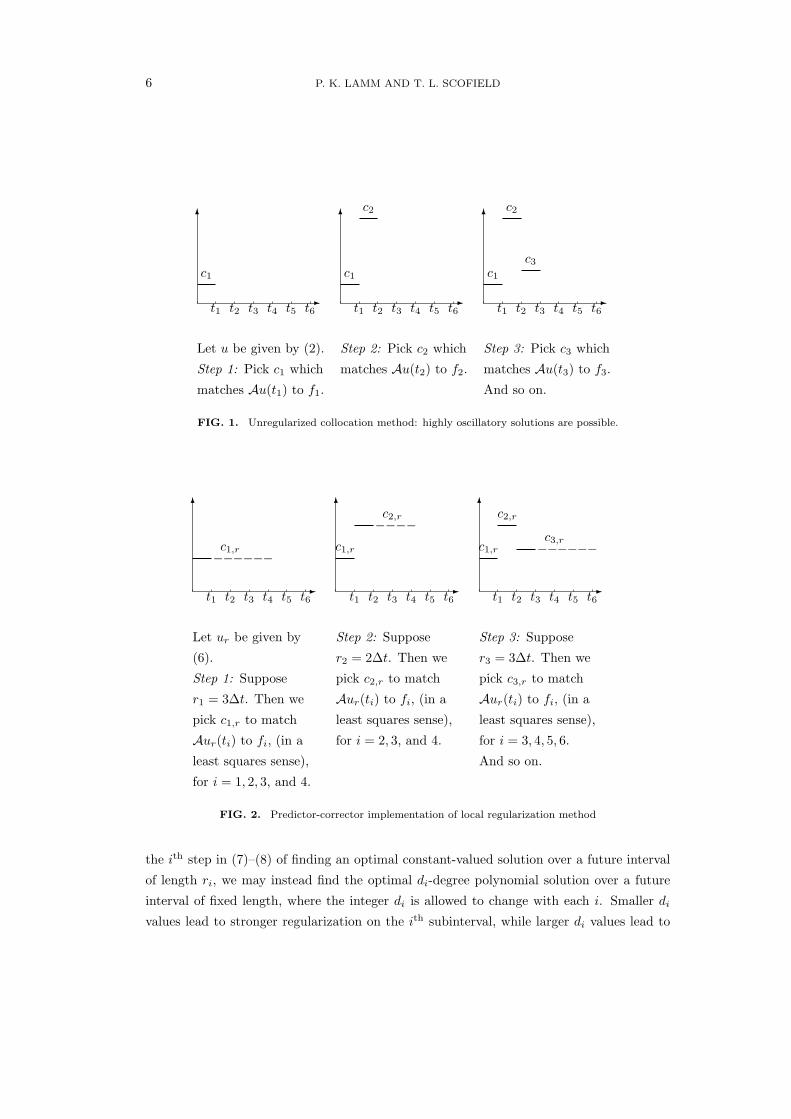
Example 2.1. In Figure 3 we first illustrate the application of standard Tikhonov

regularization for a true solution which has both steep and flat features. We show the results

for α = 0 (no regularization) and for various other choices of the Tikhonov regularization

parameter α. As can be seen from this figure, both peaks in u are adequately resolved with

the choice of α = 2.5 × 10−7, but the flat region on [.6, 1.0] is not recovered well in this

case. When α is increased in the later graphs to better handle the flat area at the end of

the interval, the first peak in u is lost due to oversmoothing. (We note that with Volterra

problems it is well-known that one cannot accurately recover values of solutions at the very

end of the interval – on say, [.8, 1.], for example – using any regularization algorithm.)Example 2.2. In Figure 4 we illustrate an application of local regularization (algorithm

(9)–(10)) to the same example. The length ri of the local interval is held constant at

ri = 2∆t = .05, for i = 1, . . . , 40, while the values of µi are changed sequentially through

the regularization process. The determination of µi is made using a sequential Morozov

discrepancy principle and knowledge of the magnitude of the error (error in the data, and

error in the propagated solution) at the ith step. Even though having good information

about the magnitude of the exact error is an unrealistic expectation, it nevertheless shows

that the sequential selection of µi has much potential for applications in which a good model

of error is available. We plot the (rescaled) µi determined by this process in the second

graph in Figure 4, connecting with line segments between discrete µi values. The general

increase in µi over the interval [0, 1] is likely to be due to the growth in propagated error

of the sequential method as the number of steps increases. It is interesting to also note the

way in which the computed µi decreases sharply near .35 and .55, roughly corresponding

to sharp increases in the true solution. The issue of sequential selection of µi is discussed

further in [27], where a simple analytic formula for µi (based on a sequential Morozov

discrepancy principle) is derived. In addition, numerical examples using non-exact error

magnitudes are also given in [27].


0.2 0.4 0.6 0.8 1

-0.5

-0.25

0.25

0.5

0.75

1

1.25alpha = .00000075

0.2 0.4 0.6 0.8 1

-0.5

-0.25

0.25

0.5

0.75

1

1.25alpha = .000001

0.2 0.4 0.6 0.8 1

-0.5

-0.25

0.25

0.5

0.75

1

1.25alpha = .00000025

0.2 0.4 0.6 0.8 1

-0.5

-0.25

0.25

0.5

0.75

1

1.25alpha = .0000005

0.2 0.4 0.6 0.8 1

-0.5

-0.25

0.25

0.5

0.75

1

1.25alpha = 0

0.2 0.4 0.6 0.8 1

-0.5

-0.25

0.25

0.5

0.75

1

1.25alpha = .0000001

FIG. 3. Tikhonov regularization for several α values (Example 2.1)


0.2 0.4 0.6 0.8 1

-0.5

-0.25

0.25

0.5

0.75

1

1.25r = .05, with computed mu

0.2 0.4 0.6 0.8 1

1.0

3.0

5.0

7.0computed mu, rescaled

FIG. 4. Local regularization with µ computed using a sequential discrepancy principle (Example 2.2)

3. A CONTINUOUS LOCAL REGULARIZATION METHOD

For suitable k and f , it can be shown [27] that the penalized predictor-corrector numer-

ical algorithm given by (9)–(10) above is simply a collocation-based discretization of the

following second-kind Volterra equation:∫ t

0

k(t, s; r)u(s) ds+ (α(t; r) + µ(t))u(t) = f(t; r), a.e. t ∈ [0, 1], (11)

where

k(t, s; r) :=∫ r(t)

0

k(t+ ρ, s) dηr(ρ; t), (12)

α(t; r) :=∫ r(t)

0

∫ ρ

0

k(t+ ρ, s+ t) ds dηr(ρ; t), (13)

f(t; r) :=∫ r(t)

0

f(t+ ρ) dηr(ρ; t), (14)

for a.e. t ∈ [0, 1]. In the above, ηr(·; t) is the r-dependent discrete measure defined for a

bounded Borel function g and a.e. t ∈ [0, 1] by∫ r(t)

0

g(ρ)dηr(ρ; t) =∫ ‖r‖∞

0

g(ρ)χ[0,r(t)](ρ) dηr(ρ; t),

where χ[0,r(t)] denotes the usual characteristic function on [0, r(t)], and where

∫ ‖r‖∞

0

g(ρ)dηr(ρ; t) :=L∑

`=1

s`(t)g(τ`), a.e. t ∈ [0, 1], (15)

with

L := 1 + max1≤i≤N

γi

s`(t) :=

{∆t− t+

∫ t`−1

−tk(t+ t`−1, t+ s) ds, 0 ≤ t ≤ ∆t,∫ t`−1

−∆tk(t+ t`−1, t+ s) ds, t > ∆t,

(16)

τ` := (`− 1)∆t,


for ` = 1 . . . , L.

For a.e. t ∈ [0, 1] the measure ηr(·; t) serves to “sample” a small amount of future data,

which is then used in the regularization process. In order for k and f in (13)–(14) to be

well-defined, we will require that both k and f be defined on an extended interval [0, T ],

for some T > 1, and that the original Volterra equation (1) holds on this extended interval

as well. (The alternative is to determine a reconstructed regularized solution of (1) on the

interval [0, 1− ε], for some ε > 0 small.)

We thus make the following standing hypothesis:

Hypothesis 3.1. For T > 1 fixed, let k ∈ C1([0, T ] × [0, T ]) and let f : [0, T ] → R be

bounded, and assume that equation (1) has a unique solution u on [0, T ]. Further, assume

k(t, t) 6= 0 for 0 ≤ t ≤ T ; without loss of generality, we assume that k(t, t) = 1 for 0 ≤ t ≤ T .

We note that in the above we assume that the kernel k satisfies k(t, t) 6= 0 for t ∈ [0, T ].

Because this assumption limits the convergence theory to those operators A for which

equation (1) is only mildly ill-posed, a couple of remarks are in order.

(1) We note that this assumption (or an assumption of even milder ill-posedness than

assumed here) is standardly found in theoretical convergence arguments for methods which

preserve the Volterra nature of the original problem. Indeed, the theory for classical regu-

larization methods is typically based on the special spectral properties of the operator A?A,

where A? is the (Hilbert) adjoint of A. However, A?A is a non-causal operator, and is thus

not of use in the theoretical treatment of methods which preserve the Volterra nature of

the original problem. For this reason, theoretical findings for Volterra-preserving methods

typically require much more stringent conditions than do classical regularization methods.

The hypotheses of several well-known Volterra-preserving methods are discussed in [24, 27].

(2) Our second comment is that the theoretical assumption k(t, t) 6= 0 does not appear

to be needed in practice for the method we present here. Indeed, as mentioned in Section

1, our method is a generalization of one which has been used for over thirty years in the

practical solution of the inverse heat conduction problem [4] (a severely ill-posed problem

for which k(t, s) and all its derivatives are zero on the line s = t). Other numerical examples

for k not satisfying the assumption k(t, t) 6= 0 may be found in [21, 27]. We note that Ring

and Prix have shown that a certain sufficient condition for convergence fails to hold for a

class of kernels k satisfying k(t, t) = 0. In [32], numerical results are given to illustrate lack

of stability for a particular example of this type; nonetheless, a change in the measure and

numerical parameters seems to restore stability. Clearly there is much work still needed

to complete our understanding of stability and convergence in the case of k(t, t) = 0. In

particular, the convergence of the method with a kernel of the class in [32] using constant-

valued r and µ = 0 is still an open problem.


3.1. A general framework for the continuous local regularization problem

For the discrete regularization algorithm described in Section 2, it was useful to prescribe

the functional regularization parameters r and µ as piecewise-constant functions. This

restriction is not needed for the continuous regularization problem so instead we generalize

the definitions of r and µ used earlier.

Definition 3.1. We define a functional regularization parameter r ∈ P, where

P := {r : [0, 1] → R : r piecewise continuous on [0, 1],with

mint∈[0,1]

r(t) > 0, maxt∈[0,1]

t+ r(t) ≤ T }.

For r ∈ P, we make the definition rmin := mint∈[0,1] r(t) > 0 and note also that ‖r‖∞ :=

maxt∈[0,1] r(t) ≤ T .

Definition 3.2. We take the penalty regularization parameter µ to be a Lebesgue-

measurable function on [0, 1] satisfying µ(t) ≥ 0 a.e. t ∈ [0, 1].

Corresponding to the generalizations of r and µ put forth in the above definitions, we

consider a larger class of measures ηr = ηr(·; t) than the one defined earlier in this section

(the one that led to the algorithm described in Section 2):

Definition 3.3. Given r ∈ P, we assume that ηr = ηr(·; t) is a Borel measure which

satisfies (15) for a.e. t ∈ [0, 1], where the r-dependent parameters L, s`, τ` satisfy

(1) L > 0 integer;

(2) s` ∈ L∞(0, 1) with 0 ≤ s`(t), a.e. t ∈ [0, 1], ` = 1, . . . , L; and,

(3) 0 ≤ τ1 < τ2 < · · · < τL ≤ ‖r‖∞, with τ` ∈ (0, rmin] and s`(t) ≥ s` > 0, for some

` = 1, . . . , L.

Given r, µ, and ηr, the continuous regularization problem is to find u = u(t; r, µ) satisfying

the second-kind Volterra equation (11).

We note that the continuous regularization equation (11) could also arise by viewing

regularization of the original Volterra problem (1) from a different perspective. Indeed we

note that, given r ∈ P, the true solution u satisfies∫ t+ρ

0

k(t+ ρ, s)u(s) ds = f(t+ ρ), a.e. ρ ∈ [0, r(t)], t ∈ [0, 1].

Splitting the left-hand side of this equation into the sum of two integrals, we have (after a

change in variables)∫ t

0

k(t+ ρ, s)u(s) ds+∫ ρ

0

k(t+ ρ, s+ t)u(s+ t) ds = f(t+ ρ), (17)


for a.e. ρ ∈ [0, r(t)], t ∈ [0, 1]. Now integrating both sides of equation (17) with respect to

the measure ηr, we get that u satisfies∫ r(t)

0

∫ t

0

k(t+ρ, s)u(s) ds dηr(ρ; t) +∫ r(t)

0

∫ ρ

0

k(t+ρ, s+t)u(s+t) ds dηr(ρ; t)

=∫ r(t)

0

f(t+ ρ) dηr(ρ; t), a.e. t ∈ [0, 1], (18)

or, after a change in order of integration in the first term of (18),∫ t

0

k(t, s; r)u(s) ds+∫ r(t)

0

∫ ρ

0

k(t+ ρ, s+ t)u(s+ t) ds dηr(ρ; t)

=∫ r(t)

0

f(t+ ρ) dηr(ρ; t), a.e. t ∈ [0, 1]. (19)

Stabilization occurs when we consider a regularized variation of (19) (which was suggested

in [22]) where the idea is to replace the second integral term in (19) by a term which serves

to restrict the variation (in some sense) of u on the local interval [t, t+ r(t)] for each t. The

result is equation (11) with µ = 0. The case of nonzero µ simply allows for a penalized

variation of this regularization problem.

In [22], consideration of equation (11) was restricted to the case of a convolution kernel,

a constant regularization parameter r(t) ≡ r, t ∈ [0, 1], and zero penalty parameter µ;

the fact that the kernel was of convolution type meant that the associated measure ηr

was necessarily t-independent. A central goal of this paper is to extend the regularized

convergence results in [22] to the case of nonconvolution kernels (which leads to the need

in practical applications for measures ηr(·; t) which depend on t), and, more importantly,

to variable regularization parameters r(·) and µ(·). The use of a variable regularization

parameter appears to allow for better resolution of solutions having sharp features, even

discontinuities, than does a constant regularization parameter. (See the numerical examples

in Section 2 and in [27].)

Remark 3.1. We note that the idea of regularizing first-kind Volterra problems via the

formulation of a related second-kind equation is not a new one. Indeed, the “small parameter

method” (see, for example, [3, 10, 18, 19, 20, 28, 36]) is based on adding a term of the form

ε(u(t)− u(0)) to the right-hand side of the original Volterra equation (1). However, for this

particular approach one requires accurate knowledge of the initial value u(0) of the true

solution, otherwise a boundary layer effect can lead to an unsatisfactory approximation of

u in the neighborhood of t = 0. See, for example, [2, 24]. In contrast, knowledge of u(0) is

not required for the local regularization method described in this paper (and in the other

local regularization references given above). The only exception to this statement is the

fairly-specific result in Theorem 4.2 below (and Theorem 5.3, which generalizes this result).

Well-posedness of equation (11) follows from the next theorem.


Theorem 3.1. Let r, µ, and ηr be given as in Definitions 3.1–3.3, and let k and f satisfy

Hypothesis 3.1. Then for ‖r‖∞ sufficiently small, there is a unique solution u(·; r, µ) ∈L2(0, 1) of equation (11) which depends continuously on f ∈ L∞(0, T ).

Proof. We may use a Taylor expansion on the integrand of α in (13) to write

α(t; r) =∫ r(t)

0

∫ ρ

0

[k(t, t) + ρD1k(t+ξ, t+ζ) + sD2k(t+ξ, t+ζ)] ds dηr(ρ; t) (20)

=

(∫ r(t)

0

ρ dηr(ρ; t)

)(1 + h(t; r)) (21)

for suitable ξ = ξt,s(ρ), ζ = ζt,s(ρ), and a.e. t ∈ [0, 1], where it follows from the definition

of ηr that∫ r(t)

0ρ dηr(ρ; t) > 0, a.e. t ∈ [0, 1]. Here

|h(t; r)| =|∫ r(t)

0

∫ ρ

0[ρD1k(t+ξ, t+ζ) + sD2k(t+ξ, t+ζ)] ds dηr(ρ; t)|∫ r(t)

0ρ dηr(ρ; t)

≤ 32‖k‖1,∞‖r‖∞, (22)

for a.e. t ∈ [0, 1]. Thus, for ‖r‖∞ sufficiently small,

α(t; r) + µ(t; r) ≥ 12

∫ r(t)

0

ρ dηr(ρ; t) > 0

for a.e. t ∈ [0, 1]. Using this fact and the assumptions on k, we have that the quantities

k(t, s; r)/(α(t; r) +µ(t; r)), 0 ≤ s ≤ t ≤ 1, and f(t; r)/(α(t; r) +µ(t; r)), 0 ≤ t ≤ 1, are well-

defined and prescribe Lebesgue square-integrable “functions” on their respective domains.

Dividing equation (11) by α(t; r) + µ(t; r), we obtain

u(t) = −∫ t

0

k(t, s; r)α(t; r) + µ(t; r)

u(s) ds+f(t; r)

α(t; r) + µ(t; r), a.e. t ∈ [0, 1], (23)

for which there is a unique solution u(·; r, µ) in L2(0, 1) depending continuously on the

quantity f(·; r)/(α(·; r) + µ(·; r)) ∈ L2(0, 1) (see, for example, [14]). It easily follows that u

depends continuously on f ∈ L∞(0, T ).

In the next section we give proofs of convergence of continuous regularization schemes

based on equation (11). Convergence results for discretizations of (11) (with formulations

generalizing the algorithms in (7)–(8) and (9)–(10)) may be found in [27]. The theoreti-

cal findings in [27] extend the results in [21] and provide an alternative to the sequential

Tikhonov regularization algorithm considered in [26].


4. CONVERGENCE RESULTS

We now turn to the issue of convergence of the regularized solution u(·; r, µ) of (11) to u

as the regularization parameters r and µ go to zero. Specifically we will look at conditions

guaranteeing ‖u(·; rn, µn) − u‖∞ → 0 as n → ∞, for appropriate sequences {rn}, {µn}satisfying ‖rn‖∞, ‖µn‖∞ → 0 as n→∞.

Once a sequence {rn} ⊂ P has been specified, we will also require a corresponding

sequence {ηrn} of measures. This is done in a natural way following Definition 3.3.

Definition 4.1. Given {rn} ⊂ P, we will define for each n = 1, 2, . . ., ηrn= ηrn

(·; t)satisfying

∫ ‖rn‖∞

0

g(ρ)dηrn(ρ; t) :=Ln∑`=1

s`,n(t)g(τ`,n), a.e. t ∈ [0, 1], (24)

where for each n = 1, 2, . . . , the parameters Ln, s`,n, and τ`,n satisfy the conditions (1)–(3)

of the corresponding (n-independent) parameters L, s`, τ`, in Definition 3.3.

Remark 4.2. Although we will not require additional conditions on {ηrn} in general, it

will be useful in certain situations to note that the practical implementation in Section 2

was naturally associated with a sequence {ηrn}, n = N = 1, 2, . . . of measures, where we

see from (15)–(16) that, in addition to the conditions given above, certain other properties

naturally occur. For example, for all n sufficiently large it follows that for this particular

sequence {ηrn} there is some L > 0 for which

Ln = L, (25)

s`,n(t) = σ`‖rn‖∞ (1 +O(‖rn‖∞)) , ` = 1, . . . , L, (26)

for a.e. t ∈ [0, 1], and

τ`,n = c`‖rn‖∞, ` = 1, . . . , L, (27)

where, for at least one ` = 1, . . . , L,

c`σ` > 0. (28)

(We note that L = 1 + ‖γ‖∞, σ` = `/‖γ‖∞, and c` = (` − 1)/‖γ‖∞ for the particular

sequence of measures associated with the practical implementation in Section 2.) We will

need conditions like these in Theorem 4.1 below.


It will be useful for the analysis in this section to make the following definition. We define

for ν = 0, 1,

aν(t; rn) :=∫ rn(t)

0

ρν dηrn(ρ, t), a.e. t ∈ [0, 1]. (29)

¿From assumptions on rn and ηrn , we note that a0(t; rn) ≥ a1(t; rn)/‖rn‖∞ > 0, a.e. t ∈[0, 1]. In addition, even if rn is a constant, aν still depends on t through the t-dependence

of ηrn.

The following technical lemma will be used to prove the main results of this section.

Lemma 4.1. For each n = 1, 2, . . ., let yn satisfy

yn(t) = −∫ t

0

(k(t, s)εn

+Kn(t, s))yn(s) ds+ En(t) + F (t), (30)

a.e. t ∈ [0, 1], where k ∈ C1([0, 1] × [0, 1]) satisfies k(t, t) = 1 for t ∈ [0, 1]; Kn(·, ·) is

bounded, measurable on [0, 1] × [0, 1]; F (·) ∈ C[0, 1] with F (0) = 0; En(·) is bounded,

measurable on [0, 1]; and where εn is a positive real number (independent of t) for each

n = 1, 2, . . .. Then yn ∈ L∞(0, 1) for each n = 1, 2, . . .. Further, if

•εn → 0,

•‖En(·)‖∞ → 0

•|Kn(t, s)| ≤M , a.e. 0 ≤ s ≤ t ≤ 1,

as n→∞, for some M > 0 independent of n, it follows that yn → 0 in L∞(0, 1) as n→∞.

Proof. The proof extends the ideas found in [22] (using a variation of an argument in [9]),

differing here in the presence of the Kn and En terms. We first note that the assumptions of

the lemma give yn ∈ L2(0, 1) [14] so that, from the form of (30) it follows that yn ∈ L∞(0, 1)

for all n.

Given εn > 0, define

ψ(t, εn) :=

{0, t < 0,

1εne−t/εn , t ≥ 0.

(31)

Convolving both sides of (30) with ψ(t, εn) we obtain∫ t

0

ψ(t− s, εn)yn(s)ds

= −∫ t

0

ψ(t− τ, εn)∫ τ

0

(k(τ, s)εn

+Kn(τ, s))yn(s) ds dτ + ψ(t, εn)∗(En(t) + F (t))

= −∫ t

0

∫ t

s

ψ(t− τ, εn)(k(τ, s)εn

+Kn(τ, s))dτ yn(s) ds+ ψ(t, εn)∗(En(t) + F (t)),


where we use an integration by parts on the first term on the right-hand side above to

obtain∫ t

0

ψ(t− s, εn)yn(s)ds

= −∫ t

0

(k(t, s)εn

− e−(t−s)/εnk(s, s)εn

)yn(s) ds+

1εn

∫ t

0

∫ t

s

e−(t−τ)/εnD1k(τ, s) dτ yn(s) ds

−∫ t

0

∫ t

s

ψ(t− τ, εn)Kn(τ, s) dτ yn(s) ds+ ψ(t, εn) ∗ (En(t) + F (t))

= −∫ t

0

(k(t, s)εn

− ψ(t− s, εn))yn(s) ds+

∫ t

0

∫ t

s

ψ(t− τ, εn)D1k(τ, s) dτ yn(s) ds

−∫ t

0

∫ t

s

ψ(t− τ, εn)Kn(τ, s) dτ yn(s) ds+ ψ(t, εn) ∗ (En(t) + F (t)),

for t ∈ [0, 1]. Subtracting the last equation from equation (30), we have for a.e. t ∈ [0, 1],

yn(t) = −∫ t

0

∫ t

s

ψ(t− τ, εn)D1k(τ, s) dτ yn(s) ds

+∫ t

0

∫ t

s

ψ(t− τ, εn)Kn(τ, s) dτ yn(s) ds−∫ t

0

Kn(t, s)yn(s) ds

+ [En(t)− ψ(t, εn) ∗ En(t)] + [F (t)− ψ(t, εn) ∗ F (t)] ,

or

yn(t) =∫ t

0

Gn(t, s)yn(s) ds+ [En(t)− ψ(t, εn) ∗ En(t)] (32)

+ [F (t)− ψ(t, εn) ∗ F (t)] , a.e. t ∈ [0, 1],

where

Gn(t, s) :=∫ t

s

ψ(t− τ, εn) (Kn(τ, s)−D1k(τ, s)) dτ −Kn(t, s)

for 0 ≤ s ≤ t ≤ 1. But

|Gn(t, s)| ≤∫ t

s

e−(t−τ)/εn

εn(|Kn(τ, s)|+ |D1k(τ, s)|) dτ + |Kn(t, s)|

≤ (‖k‖1,∞ +M)(1− e−(t−s)/εn

)+M

≤ ‖k‖1,∞ + 2M,

for a.e. 0 ≤ s ≤ t ≤ 1. Further, for a.e. t ∈ [0, 1],

En(t)− ψ(t, εn) ∗ En(t) ≤ ‖En(·)‖∞[1 +

∫ t

0

ψ(t− τ, εn) dτ]

≤ 2‖En(·)‖∞.

Combining these estimates with equation (32), we see that for a.e. t ∈ [0, 1],

|yn(t)| ≤∫ t

0

(‖k‖1,∞ + 2M) |yn(s)| ds+ 2‖En(·)‖∞

+ |F (t)− ψ(t, εn) ∗ F (t)| . (33)


Finally we use the result [9, 12] that if g : [0, 1] → R is a continuous function satisfying

g(0) = 0, then ψ(t, ε) ∗ g(t) → g(t) as ε→ 0+, uniformly in t ∈ [0, 1]. We thus have that

|F (t)− ψ(t, εn) ∗ F (t)| → 0

as n→∞, uniformly in t ∈ [0, 1]. An application of a generalized Gronwall inequality (see,

e.g., [34, 37]) to the bound in (33) completes the proof of the lemma.

4.1. Convergence with constant r and variable µ

We obtain convergence results in this section as the regularization parameters go to zero,

for functional parameters µn and constant parameters rn; the same results hold for nearly

constant rn, as will be seen in Section 5. For the result that follows we also require the

additional conditions (25)–(28) on {ηrn}, conditions which occur naturally in practice.

Theorem 4.1. Assume that u ∈ C1[0, 1]. Let {rn} ⊂ R be a given sequence with rn → 0

as n→∞. Assume that the rn-dependent measures ηrnare given as in Definition 4.1 and

such that the additional conditions (25)–(28) hold.

Then if, for some Cµ ≥ 0 and p ≥ 3, {µn} ⊂ L∞(0, 1) is selected satisfying

0 ≤ µn(t) ≤ Cµrpn, a.e. t ∈ [0, 1], (34)

for all n sufficiently large, it follows that u(·; rn, µn), the solution of∫ t

0

k(t, s; rn)u(s) ds+ [α(t; rn) + µn(t)]u(t) = f(t; rn), a.e. t ∈ [0, 1], (35)

belongs to L∞(0, 1) and converges to u in L∞(0, 1) as n→∞.

Moreover, if the sequence {fδn} ∈ L∞(0, T ) is given with dn(t) := fδn(t)− f(t), a.e. t ∈[0, 1], n = 1, 2, . . ., where for a.e. t ∈ [0, 1], |dn(t)| ≤ δn → 0 as n → ∞, then the solution

uδn(·; rn, µn) ∈ L∞(0, 1) of∫ t

0

k(t, s; rn)u(s) ds+ [α(t; rn) + µn(t)]u(t) = fδn(t; rn), a.e. t ∈ [0, 1], (36)

converges to u in L∞(0, 1) as n→∞, provided that rn = rn(δn) is chosen so that

δnrn(δn)

→ 0

and rn(δn) → 0 as n→∞. In (36), fδn is defined by

fδn(t; rn) :=∫ rn

0

fδn(t+ ρ) dηrn(ρ; t).


Proof. ¿From (19), the true solution u of (1) satisfies∫ t

0

k(t, s; rn)u(s) ds+ [α(t; rn) + µn(t)] u(t)

=∫ rn

0

f(t+ ρ) dηrn(ρ; t) + µn(t)u(t), (37)

−∫ rn

0

∫ ρ

0

k(t+ ρ, s+ t) [u(s+ t)− u(t)] ds dηrn(ρ; t),

for a.e. t ∈ [0, 1]. Setting yδn(t; rn, µn) := uδn(t; rn, µn)−u(t), for uδn(·; rn, µn) the solution

of (36), we see that yδn(t; rn, µn) solves

yn(t) =−1

α(t; rn) + µn(t)

∫ t

0

k(t, s; rn)yn(s) ds+ E(t; rn) + F (t; rn), (38)

for a.e. t ∈ [0, 1] and n = 1, 2, . . ., where

E(t; rn) :=

∫ rn

0dn(t+ ρ) dηrn

(ρ; t)α(t; rn) + µn(t)

, (39)

F (t; rn) :=

∫ rn(t)

0

∫ ρ

0k(t+ ρ, s+ t) [u(s+ t)− u(t)] ds dηrn

(ρ; t)− µn(t)u(t)α(t; rn) + µn(t)

, (40)

a.e. t ∈ [0, 1], and where E(·; rn) = 0 for all n in the case of noise-free data f .

A Taylor expansion may be used to write (for suitable νt,s(ρ)),

k(t, s; rn) =∫ rn

0

k(t+ ρ, s) dηrn(ρ; t)

=∫ rn

0

[k(t, s) + ρD1k(t+ νt,s(ρ), s)] dηrn(ρ; t),

a.e. 0 ≤ s ≤ t ≤ 1, so that

k(t, s; rn) = a0(t; rn)k(t, s) +∫ rn

0

ρD1k(t+ νt,s(ρ), s) dηrn(ρ; t), (41)

for a.e. 0 ≤ s ≤ t ≤ 1, where a0 is defined in (29). Similarly, (21) and (22) give

α(t; rn) = a1(t; rn)(1 + h(t; rn)), a.e. t ∈ [0, 1],

where |h(t; rn)| ≤ 32‖k‖1,∞‖rn‖∞ for a.e. t ∈ [0, 1], so that

α(t; rn) + µn(t) = a1(t; rn)(

1 +µn(t)a1(t; rn)

+ h(t; rn)), a.e. t ∈ [0, 1].

If we pick µn(t) ≥ 0, a.e. t ∈ [0, 1], satisfying (34), then (25)–(28) guarantee that, for all rnsufficiently small,

1α(t; rn) + µn(t)

=1

a1(t; rn)(1 + g(t; rn)) ,


where ‖g(·; rn)‖∞ = O(rn). Conditions (25)–(28) on ηrn also give us that

a1(t, rn)a0(t, rn)

= κrn(1 +O(rn)), a.e. t ∈ [0, 1], (42)

where

κ =∑L

`=1 c`σ`∑L`=1 σ`

> 0.

The kernel in (38) may then be estimated by

k(t, s; rn)α(t; rn) + µn(t)

=a0(t; rn)a1(t; rn)

(1 + g(t; rn)) k(t, s) +D(t, s; rn)

=1κrn

(1 +O(rn))k(t, s) +D(t, s; rn), (43)

for a.e. 0 ≤ s ≤ t ≤ 1, where

|D(t, s; rn)| :=∣∣∣∣1 + g(t; rn)a1(t; rn)

∫ rn

0

ρD1k(t+ νt,s(ρ), s) dηrn(ρ; t)∣∣∣∣

≤ 1 + |g(t; rn)|a1(t; rn)

∫ rn

0

ρ |D1k(t+ νt,s(ρ), s)| dηrn(ρ; t)

≤ ‖k‖1,∞[1 + |g(t; rn)|]

≤ 2‖k‖1,∞,

for rn sufficiently small and a.e. 0 ≤ s ≤ t ≤ 1. Thus

k(t, s; rn)α(t; rn) + µn(t)

=k(t, s)εn

+Kn(t, s), 0 ≤ s ≤ t ≤ 1,

where εn := κrn → 0 as n→∞, and

Kn(t, s) :=γ(t; rn)k(t, s)

κrn+D(t, s; rn)

is bounded, a.e. 0 ≤ s ≤ t ≤ 1, as n→∞. In addition, for all rn sufficiently small and for

a.e. t ∈ [0, 1],

|E(t; rn)| ≤∫ rn

0|dn(t+ ρ)| dηrn(ρ; t)

a1(t; rn)(1 + |g(t; rn)|)

≤ 2δna0(t; rn)a1(t; rn)

≤ 4δn/(κrn),

for rn sufficiently small, from the assumptions of the theorem. Further,

|F (t; rn)|

≤

(∫ rn

0

∫ ρ

0k(t+ρ, s+t) |u(s+t)− u(t)| ds dηrn(ρ; t) + µn(t)|u(t)|

a1(t; rn)

)(1 + |g(t; rn)|)


≤ 2‖k‖∞‖u‖1,∞

∫ rn

0

∫ ρ

0s ds dηrn(ρ; t)a1(t; rn)

+ 2‖u‖∞µn(t)a1(t; rn)

= O(rn)

for rn sufficiently small and a.e. t ∈ [0, 1].

Thus yδn(·, rn, µn) satisfies the conditions of Lemma 4.1, i.e., yδn(·, rn, µn) satisfies

yn(t) = −∫ t

0

(k(t, s)εn

+Kn(t, s))yn(s) ds+ En(t), a.e. t ∈ [0, 1],

where En(t) := E(t; rn)+F (t; rn) satisfies ‖En‖∞ → 0 as n→∞ under the assumptions in

the theorem. The result then follows from Lemma 4.1.

4.2. Convergence with variable r and fixed µ

We turn to a second result which allows rn to vary with t and places fewer constraints on

ηrn than did Theorem 4.1; however, this improvement occurs at the expense of requiring a

fixed (rn-dependent) construction of µn.

Theorem 4.2. Assume that u ∈ C[0, T ] with u(0) = 0. Let {rn(·)} ⊂ P be given with

rn → 0 as n → ∞, uniformly on [0, 1], and assume that the sequence {ηrn} of measures is

defined as usual from {rn} using Definition 4.1.

If µn = µn(·; rn) is given by

µn(t; rn) := Cµ‖rn‖p∞

∫ rn(t)

0

dηrn(ρ; t), t ∈ [0, 1], (44)

for some p ∈ (0, 1/2] and Cµ > 0, then the solution u(·; rn, µn) ∈ L∞(0, 1) of (35) converges

to u(·) in L∞(0, 1) as n→∞. Moreover, if fδn satisfies the conditions of Theorem 4.1, then

the solution uδn(·; rn, µn) of (36) converges to u in L∞(0, 1), provided that rn(·) = rn(·; δn)

is chosen so thatδn

‖rn(·; δn)‖p∞→ 0

and ‖rn(·; δn)‖∞ → 0 as n→∞.

Proof. As in the proof of Theorem 4.1, the error function yδn(·; rn) = uδn(·; rn, µn)−u(·)satisfies (38) for n = 1, 2, . . ., where now µn(t) = µn(t; rn) is given by (44). Further, from

(41) we may write

k(t, s; rn) = a0(t; rn) [k(t, s) +H(t, s; rn)] , a.e. 0 ≤ s ≤ t ≤ 1, (45)

where

|H(t, s; rn)| =

∣∣∣∫ rn(t)

0ρD1k(t+ νt,s(ρ), s)dηrn

(ρ; t)∣∣∣

a0(t; rn)


≤ ‖k‖1,∞‖rn‖∞,

for a.e. 0 ≤ s ≤ t ≤ 1. Employing a Taylor expansion as in (20), we obtain

α(t; rn) = Cµ ‖rn‖p∞ a0(t; rn) h(t; rn), a.e. t ∈ [0, 1],

for Cµ and p given in (44) and where, for a.e. t ∈ [0, 1],

∣∣∣h(t; rn)∣∣∣ =

∣∣∣∫ rn(t)

0

∫ ρ

0[1 + ρD1k(t+ ξ, t+ ζ) + sD2k(t+ ξ, t+ ζ)] ds dηrn(ρ; t)

∣∣∣Cµ‖rn‖p

∞ a0(t; rn)

≤ 1Cµ‖rn‖p

∞ a0(t; rn)

[‖rn‖∞a0(t; rn) +

32‖k‖1,∞

∫ rn(t)

0

ρ2 dηrn(ρ; t)

]

≤ ‖rn‖1−p∞

Cµ

[1 +

32‖k‖1,∞‖rn‖∞

]= O(‖rn‖1−p

∞ )

as ‖rn‖∞ → 0. Thus using this estimate and the definition of µn(·; rn) given in (44),

1α(t; rn) + µn(t; rn)

=1

Cµ‖rn‖p∞ a0(t; rn)

· 11 + h(t; rn)

=1 + γp(t; rn)

Cµ‖rn‖p∞ a0(t; rn)

, a.e. t ∈ [0, 1], (46)

for ‖rn‖∞ sufficiently small, where ‖γp(·; rn)‖∞ = O(‖rn‖1−p∞ ) as ‖rn‖∞ → 0.

Using (45) and (46), it follows that the solution yn of (38) satisfies

yn(t) = −1 + γp(t; rn)Cµ‖rn‖p

∞

∫ t

0

[k(t, s) +H(t, s; rn)] yn(s) ds+ E(t; rn) + F (t; rn)

= −∫ t

0

[k(t, s)

Cµ‖rn‖p∞

+G(t, s; rn)]yn(s) ds+ E(t; rn) + F (t; rn), (47)

for a.e. t ∈ [0, 1], where E and F are given by (39) and (40), respectively (with E ≡ 0

when noise-free data f is used), and where for a.e. 0 ≤ s ≤ t ≤ 1,

|G(t, s; rn)| = 1Cµ‖rn‖p

∞|k(t, s)γp(t; rn) +H(t, s; rn) [1 + γp(t; rn)] | .

The terms in G are of order ‖rn‖1−2p∞ and ‖rn‖1−p

∞ , respectively, and since p ∈ (0, 1/2], it

follows that ‖G(·, ·; rn)‖∞ = O(1) as n→∞.

Thus we may apply Lemma 4.1 with Kn(t, s) = G(t, s; rn), εn = Cµ‖rn‖p∞, and En(·),

F (·) given in (30) by

En(t) =

∫ rn(t)

0

∫ ρ

0k(t+ ρ, s+ t) [u(s+ t)− u(t)] ds dηrn(ρ; t) + α(t; rn)u(t)

α(t; rn) + µn(t; rn)

+

∫ rn(t)

0dn(t+ ρ) dηrn(ρ; t)

α(t; rn) + µn(t; rn),

F (t) = −u(t),


for a.e. 0 ≤ t ≤ 1. In bounding En, we have from (46) that for a.e. t ∈ [0, 1],∣∣∣∫ rn(t)

0

∫ ρ

0k(t+ ρ, s+ t) [u(s+ t)− u(t)] ds dηrn

(ρ; t) + α(t; rn)u(t)∣∣∣

α(t; rn) + µn(t; rn)

≤ 3α(t; rn)α(t; rn) + µn(t; rn)

‖u‖∞

≤ 3α(t; rn)µn(t; rn)

‖u‖∞

= 3h(t; rn)‖u‖∞

= O(‖rn‖1−p∞ ).

Finally, the last term in En(t) is bounded for 0 ≤ t ≤ 1 by∣∣∣∣∣∫ rn(t)

0dn(t+ ρ)dηrn

(ρ; t)α(t; rn) + µn(t; rn)

∣∣∣∣∣ ≤ δna0(t; rn)µn(t; rn)

= δna0(t; rn)

Cµ‖rn‖p∞a0(t; rn)

.

Thus, under the conditions of the theorem we have ‖En‖∞ → 0 as n → ∞. An appli-

cation of Lemma 4.1 then gives that uδn(·; rn, µn) converges to u in L∞(0, 1) as n→∞.

5. CONTINUOUS LOCAL REGULARIZATION WITH GENERAL

MEASURES

Finally we turn to a generalization of the theory developed earlier, here allowing the

measure ηr to take a more general form. The discrete measure defined in preceding sections

will be a special case of the general measure we construct here; in addition, the theory

of this section will apply to measures of the form given in Example 5.1 below. Although

the generalization of the theory in Sections 3–4 leads to more technical definitions and

theoretical results, the proofs of these results are quite similar to those given in the preceding

sections (see also [35]). We will state the relevant theorems below without proof.

In the generalization we will let f ∈ FD, the admissible set of data functions, where it is

assumed that all g ∈ FD are bounded Borel functions on [0, 1].

Definition 5.1. For given r ∈ P, we say that the one-parameter family Nr =

{ηr(·; t), t ∈ [0, 1]} is an r-suitable family of measures if, for a.e. t ∈ [0, 1], ηr(·; t) is a

finite positive Borel measure on [0, r(t)], and the family Nr is such that the following three

conditions hold:

(1)∫ r(t)

0ρ dηr(ρ; t) > 0, a.e. t ∈ [0, 1];

(2) the quantities k(·, ·; r), α(·; r), and f(·; r), defined by (12), (13), and (14), respectively,

are Lebesgue measurable on their respective domains (for all f ∈ FD); and


(3) t 7→∫ r(t)

0dηr(ρ; t)∫ r(t)

0ρ dηr(ρ; t)

∈ L2(0, 1).

As indicated above, given r ∈ P the family Nr = {ηr(·; r), t ∈ [0, 1]}, where ηr is given by

Definition 3.3, is an r-suitable family of measures. Another example of an r-suitable family

of measures is as follows.

Example 5.1. Let r ∈ P be given, and let ωr ∈ L∞( (0, ‖r‖∞) × (0, T ) ) be given with

0 < ωr ≤ ωr(ρ, t), a.e. ρ ∈ (0, ‖r‖∞), t ∈ (0, T ). Define Nr = {ηr(·; r), t ∈ [0, 1]}, where∫ ‖r‖∞

0

g(ρ)dηr(ρ; t) :=∫ ‖r‖∞

0

g(ρ)ωr(ρ, t)dρ, a.e. t ∈ [0, 1],

for g a bounded Borel function. Then Nr is an an r-suitable family of measures.

When ηr takes a more general form than that assumed in previous sections, we still

obtain the existence of solutions u(·; r, µ) of equation (11). The next theorem states this

result precisely, with proof similar to that of Theorem 3.1.

Theorem 5.1. Given r ∈ P, let Nr = {ηr(·; t), t ∈ [0, 1]} be an r-suitable family of

measures and let µ be given as in Definition 3.2. Assume that k and f ∈ FD satisfy

Hypothesis 3.1. Then for ‖r‖∞ sufficiently small, there is a unique solution u(·; r, µ) ∈L2(0, 1) of equation (11) which depends continuously on f ∈ L∞(0, 1).

Analogous to Theorem 4.1, we obtain convergence of regularized solutions to the true so-

lution u, provided the regularization parameter r is “nearly constant” (this requirement can

be seen to follow from condition (48) below), while the functional regularization parameter

µ need only satisfy a weak size condition (49) relative to r.

Theorem 5.2. Assume that u ∈ C1[0, 1]. Let {rn} ⊂ P be a given sequence with rn →0 as n → ∞, uniformly on [0, 1], and for each n = 1, 2, . . ., let Nrn denote a family

{ηrn(·; t), t ∈ [0, 1]} of rn-suitable measures. Assume that there is κn : R+ → R+ for which

a1(t, rn)a0(t, rn)

= κn(‖rn‖∞) (1 +O(‖rn‖∞)) , a.e. t ∈ [0, 1], (48)

as ‖rn‖∞ → 0, where, for some mκ > 0, κn satisfies κn(‖rn‖∞) ≥ mκ‖rn‖∞ for all n

sufficiently large, and κn(‖rn‖∞) → 0 as n→∞.

Then if, for some Cµ ≥ 0 and p ≥ 1, µn(·) is selected satisfying µn(t) ≥ 0, a.e. t ∈ [0, 1],

and

µn(t) ≤ Cµ‖rn‖p∞

∫ rn(t)

0

ρ dηrn(ρ; t), a.e. t ∈ [0, 1], (49)


for all n sufficiently large, it follows that u(·; rn, µn), the solution of (35), belongs to L∞(0, 1)

and converges to u in L∞(0, 1) as n→∞.

Moreover, if the sequence {fδn} ⊂ FD is given with dn(t) := fδn(t)− f(t), a.e. t ∈ [0, 1],

n = 1, 2, . . ., where for a.e. t ∈ [0, 1], |dn(t)| ≤ δn → 0 as n → ∞, then the solution

uδn(·; rn, µn) ∈ L∞(0, 1) of (36) converges to u in L∞(0, 1) as n → ∞, provided that

rn(·) = rn(·; δn) is chosen so that

δn‖rn(·; δn)‖∞

→ 0

and ‖rn(·; δn)‖∞ → 0 as n→∞.

Finally, when we relax restrictions on the r regularization parameter, we obtain conver-

gence provided we make a precise definition of the µ regularization parameter. This result

is a generalization of Theorem 4.2.

Theorem 5.3. Assume that u ∈ C[0, T ] with u(0) = 0. Let {rn(·)} ⊂ P be given with

rn → 0 as n→∞, uniformly on [0, 1], and assume that, for each n = 1, 2, . . ., we have an

rn-suitable family Nr = {ηrn(·; t), t ∈ [0, 1]} of measures. If µn = µn(·; rn) is given by

µn(t; rn) := Cµ‖rn‖p∞

∫ rn(t)

0

dηrn(ρ; t), t ∈ [0, 1],

for some p ∈ (0, 1/2] and Cµ > 0, then the solution u(·; rn, µn) ∈ L∞(0, 1) of (35) converges

to u(·) in L∞(0, 1) as n→∞. Moreover, if fδn satisfies the conditions of Theorem 4.1, then

the solution uδn(·; rn, µn) of (36) converges to u in L∞(0, 1), provided that rn(·) = rn(·; δn)

is chosen so that

δn‖rn(·; δn)‖p

∞→ 0

and ‖rn(·; δn)‖∞ → 0 as n→∞.

6. CONCLUSION

We have presented theoretical convergence results for a local regularization method ap-

plied to ill-posed Volterra problems of the form (1). This method extends the ideas in [22]

to the case of a local regularization parameter r which is allowed to vary over different parts

of the domain, and to Volterra problems with nonconvolution kernels (which, in practice,

means that t-dependent families {ηr(·; t), t ∈ [0, 1]} of measures must be considered). In

addition to allowing variability in r, we have considered the inclusion of a second variable

regularization parameter µ which serves to further restrict the variation of regularized solu-

tions. Numerical results indicate that, for fixed regularization parameter r, the parameter


µ may be determined using a local (sequential) Morozov discrepancy principle provided one

has a good estimate of the data error and propagated error. A more extensive discussion

of this sequential discrepancy principle and analysis of the convergence of a discrete local

regularization method (based on the ideas of this paper) may be found in [27].

ACKNOWLEDGMENTThis work was supported in part by the National Science Foundation under contract number

NSF DMS 9704899 (P.K.L.)

REFERENCES1. R. Acar and C. Vogel, Analysis of bounded variation penalty methods for ill-posed problems, Inverse

Problems, 10 (1994), pp. 1217–1229.

2. J. S. Angell and W. E. Olmstead, Singularly perturbed Volterra integral equations, SIAM J. Appl. Math.,47 (1987), pp. 1–14.

3. A. Asanov, A class of systems of Volterra integral equations of the first kind, Funktsional. Anal. iPrilozhen., 17 (1983), pp. 73–74; English translation: Functional Analysis and its Applications, 17,pp. 303–4.

4. J. V. Beck, B. Blackwell and C. R. St. Clair, Jr., Inverse Heat Conduction, Wiley-Interscience, NewYork, 1985.

5. G. Blanc, J. V. Beck and M. Raynaud, Solution of the inverse heat conduction problem with a time-variable number of future temperatures, Numerical Heat Transfer, Part B, 32 (1997), pp. 437–451.

6. T. A. Burton, Volterra Integral and Differential Equations, Academic Press, New York, 1983.

7. A. Chambolle and P.-L. Lions, Image recovery via total variation minimization and related problems,Numer. Math., 72 (1997), pp. 167–188.

8. A. C. Cinzori and P. K. Lamm, Future polynomial regularization of first-kind Volterra operators, SIAMJ. Numerical Analysis, to appear.

9. C. Corduneanu, Integral Equations and Applications, Cambridge University Press, Cambridge, 1991.

10. A. M. Denisov, The approximate solution of a Volterra equation of the first kind, Z. Vycisl. Mat. iMat. Fiz., 15 (1975), pp. 1053–1056, 1091; English translation: USSR Comput. Math. Math. Phys., 15,pp. 237–239.

11. D. C. Dobson and C. R. Vogel, Convergence of an iterative method for total variation denoising, SIAMJ. Numerical Analysis, 34 (1997), pp. 1779-1971.

12. R. E. Edwards, Fourier Series (a Modern Introduction), Vol. 1, 2nd Ed., Springer-Verlag, Berlin, 1979.

13. H. W. Engl, M. Hanke and A. Neubauer, Regularization of Inverse Problems, Kluwer Academic Pub-lishers, Dordrecht, The Netherlands, 1996.

14. G. Gripenberg, S. O. Londen and O. Saffens, Volterra Integral and Functional Equations, CambridgeUniversity Press, Cambridge, 1990.

15. C. W. Groetsch, The Theory of Tikhonov Regularization for Fredholm Equations of the First Kind,Pitman, Boston, 1984.

16. K. Ito and K. Kunisch, An active set strategy based on the augmented Lagrangian formulation for imagerestoration, R.A.I.R.O. Math. Mod. and Numer. Anal., to appear.

17. K. Ito and K. Kunisch, Augmented Lagrangian formulation of nonsmooth convex optimization in Hilbertspaces, in Control of Partial Differential Equations and Applications, Proceedings of the IFIP TC7/WG-7.2 International Conference, Laredo, Spain, 1994, Lect. Notes Pur Appl. Math. 174, E. Casas, ed.,Dekker, New York (1996), pp. 107–117.

18. M. I. Imanaliev and A. Asanov, Solutions of systems of nonlinear Volterra integral equations of the firstkind, Dokl. Akad. Nauk SSSR, 309 (1989), pp. 1052–1055; English translation: Soviet Math. Dokl., 40,pp. 610–613.

19. M. I. Imanaliev, B. V. Khvedelidze, T. G. Gegeliya, A. A. Babaev and A. I. Botashev, Integral equations,Differential Equations, 18 (1982), pp. 1442–1458.


20. B. Imomnazarov, Regularization of dissipative operator equations of the first kind, Zh. Vychisl. Mat. iMat. Fiz., 22 (1982), pp. 791–800, 1019; English translation: USSR Comput. Math. Math. Phys., 22,pp. 22-32.

21. P. K. Lamm, Approximation of ill-posed Volterra problems via predictor–corrector regularization meth-ods, SIAM J. Appl. Math., 56 (1996), pp. 524–541.

22. P. K. Lamm, Future-sequential regularization methods for ill-posed Volterra equations: applications tothe inverse heat conduction problem, J. Math. Anal. Appl., 195 (1995), pp. 469–494.

23. P. K. Lamm, Regularized inversion of finitely smoothing Volterra operators: predictor–corrector regu-larization methods, Inverse Problems, 13 (1997), pp. 375–402.

24. P. K. Lamm, A survey of regularization methods for first-kind Volterra equations, to appear.

25. P. K. Lamm, On the local regularization of inverse problems of Volterra type, in Proc. 1995 ASMEDesign Engineering Technical Conferences – Parameter Identification Symposium, Boston, MA, 1995.

26. P. K. Lamm, P. K and L. Elden, Numerical solution of first-kind Volterra equations by sequentialTikhonov regularization, SIAM J. Numer. Anal., 34 (1997), pp. 1432–1450.

27. P. K. Lamm and T. L. Scofield, Sequential predictor-corrector methods for the variable regularizationof Volterra problems, Inverse Problems, 16 (2000), pp. 373–399.

28. N. A. Magnickiı, The approximate solution of certain Volterra integral equations of the first kind,Vestnik Moskov. Univ. Ser. XV Vycisl. Mat. Kibernet., 1978 pp. 91–96; English translation: MoscowUniv. Comput. Math. Cybernetics, 1978, pp. 74–78.

29. J. C. Munoz and Y. L. Yeow, Applications of maximum entropy method in capillary viscometry,Rheo. Acta, 35 (1996), pp. 76–82.

30. M. Z. Nashed and O. Scherzer, Least squares and bounded variation regularization with nondifferentiablefunctionals, Numer. Funct. Anal. and Optimz., 19 (1998), pp. 873–901.

31. A. Neubauer and O. Scherzer, Regularization for curve representations: uniform convergence for discon-tinuous solutions of ill-posed problems, SIAM J. Appl. Math., 58 (1998), pp. 1891–1900.

32. W. Ring and J. Prix, Sequential predictor-corrector regularization methods and their limitations, InverseProblems, 16 (1999), pp. 619–634.

33. L. I. Rudin, S. Osher and E. Fatemi, Nonlinear total variation based noise removal algorithms, PhysicaD, 60 (1992), pp. 259–268.

34. S. Schwabik, Generalized Ordinary Differential Equations, World Scientific Publ. Co., New Jersey, 1992.

35. T. L. Scofield, Sequential predictor-corrector methods for variable regularization of ill-posed Volterraproblems, Ph.D. Thesis (1998), Department of Mathematics, Michigan State University, E. Lansing, MI48824–1027.

36. V. O. Sergeev, Regularization of Volterra equations of the first kind, Dokl. Akad. Nauk SSSR, 197(1971), pp. 531–534; English translation: Soviet Math. Dokl., 12, pp. 501–505.

37. D. Willett, A linear generalization of Gronwall’s inequality, Proc. Amer. Math. Soc., 16 (1965), pp. 774–778.

LOCAL REGULARIZATION METHODS FOR THE STABILIZATION...

Documents

Transcript of LOCAL REGULARIZATION METHODS FOR THE STABILIZATION...