Local polynomial chaos expansion method for high ...

Purdue UniversityPurdue e-Pubs

Open Access Dissertations Theses and Dissertations

8-2016

Local polynomial chaos expansion method for highdimensional stochastic differential equationsYi ChenPurdue University

Follow this and additional works at: https://docs.lib.purdue.edu/open_access_dissertations

Part of the Applied Mathematics Commons

This document has been made available through Purdue e-Pubs, a service of the Purdue University Libraries. Please contact [email protected] foradditional information.

Recommended CitationChen, Yi, "Local polynomial chaos expansion method for high dimensional stochastic differential equations" (2016). Open AccessDissertations. 744.https://docs.lib.purdue.edu/open_access_dissertations/744

https://docs.lib.purdue.edu?utm_source=docs.lib.purdue.edu%2Fopen_access_dissertations%2F744&utm_medium=PDF&utm_campaign=PDFCoverPages

https://docs.lib.purdue.edu/open_access_dissertations?utm_source=docs.lib.purdue.edu%2Fopen_access_dissertations%2F744&utm_medium=PDF&utm_campaign=PDFCoverPages

https://docs.lib.purdue.edu/etd?utm_source=docs.lib.purdue.edu%2Fopen_access_dissertations%2F744&utm_medium=PDF&utm_campaign=PDFCoverPages

https://docs.lib.purdue.edu/open_access_dissertations?utm_source=docs.lib.purdue.edu%2Fopen_access_dissertations%2F744&utm_medium=PDF&utm_campaign=PDFCoverPages

http://network.bepress.com/hgg/discipline/115?utm_source=docs.lib.purdue.edu%2Fopen_access_dissertations%2F744&utm_medium=PDF&utm_campaign=PDFCoverPages

https://docs.lib.purdue.edu/open_access_dissertations/744?utm_source=docs.lib.purdue.edu%2Fopen_access_dissertations%2F744&utm_medium=PDF&utm_campaign=PDFCoverPages

Graduate School Form 30 Updated ��

PURDUE UNIVERSITY GRADUATE SCHOOL

Thesis/Dissertation Acceptance

This is to certify that the thesis/dissertation prepared

By

Entitled

For the degree of

Is approved by the final examining committee:

To the best of my knowledge and as understood by the student in the Thesis/Dissertation Agreement, Publication Delay, and Certification Disclaimer (Graduate School Form 32), this thesis/dissertation adheres to the provisions of Purdue University’s “Policy of Integrity in Research” and the use of copyright material.

Approved by Major Professor(s):

Approved by: Head of the Departmental Graduate Program Date

YI CHEN

LOCAL POLYNOMIAL CHAOS EXPANSION METHOD FOR HIGH DIMENSIONAL STOCHASTIC DIFFERENTIAL EQUATIONS

Doctor of Philosophy

Dongbin XiuCo-chair

Suchuan Dong Co-chair

Peijun Li

Guang Lin

Dongbin Xiu

David Goldberg 6/6/2016

LOCAL POLYNOMIAL CHAOS EXPANSION METHOD

FOR HIGH DIMENSIONAL STOCHASTIC DIFFERENTIAL EQUATIONS

A Dissertation

Submitted to the Faculty

of

Purdue University

by

Yi Chen

In Partial Fulfillment of the

Requirements for the Degree

of

Doctor of Philosophy

August 2016

Purdue University

West Lafayette, Indiana

ii

To my beloved ones:

my parents, my grandparents, and many others.

iii

ACKNOWLEDGMENTS

First of all, I would like to express my deepest gratitude to my major advisor, Prof.

Dr. Dongbin Xiu. I appreciate all his contributions of time, wisdom and funding that

result in a productive and stimulating Ph.D. experience for me. I was motivated by

his enthusiasm and creativity in research. He also serves as a role model to me as a

member of academia.

I would like to thank Prof. Suchuan Dong, Prof. Peijun Li and Prof. Guang Lin

for serving as committee members for the past a few years. Special thanks to Prof.

Suchuan Dong for being the co-chair of the committe while Prof. Dongbin Xiu is in

Utah. Their guidance has served me well and greatly improved the quality of my

dissertation.

I wish to acknowledge the help provided by Dr. Claude Gittelson and Dr. John

Jakeman for the work to overcome the challenges in local polynomial chaos method-

ology and numerical experiments. This work became my first published paper.

Dr. Xueyu Zhu deserve my sincere thanks for providing insightful comments

and contributions to the work of validations of local polynomial chaos methodol-

ogy. Together, we draw the connection between strategies of stochastic PDEs and

deterministic PDEs. This work becames the highlight of my research.

I would like to thank all my colleagues in Mathematics Department. Shuhao Cao,

Xuejing Zhang and Jing Li are the ones who provided guidance and help in di↵erent

research areas. Many thanks to my formal roommate Nan Ding and Xiaoxiao Chen

and many other friends for the help and support when I was having health issues in

2013.

Finally, I would like to say thanks to my beloved ones. This thesis is dedicated to

them.

iv

TABLE OF CONTENTS

Page

LIST OF FIGURES . . . . . . . . . . . . . . . . . . . . . . . . . . . . . . . vi

ABBREVIATIONS . . . . . . . . . . . . . . . . . . . . . . . . . . . . . . . . ix

ABSTRACT . . . . . . . . . . . . . . . . . . . . . . . . . . . . . . . . . . . x

1 INTRODUCTION . . . . . . . . . . . . . . . . . . . . . . . . . . . . . . 11.1 Overview . . . . . . . . . . . . . . . . . . . . . . . . . . . . . . . . . 11.2 Preliminaries . . . . . . . . . . . . . . . . . . . . . . . . . . . . . . 3

1.2.1 Generalized Polynomial Chaos . . . . . . . . . . . . . . . . . 41.2.2 Stochastic Galerkin Method . . . . . . . . . . . . . . . . . . 61.2.3 Stochastic Collocation Method . . . . . . . . . . . . . . . . . 7

1.3 Research Outline . . . . . . . . . . . . . . . . . . . . . . . . . . . . 13

2 LOCALIZED POLYNOMIAL CHAOS METHODOLOGY . . . . . . . . 152.1 Problem Setup . . . . . . . . . . . . . . . . . . . . . . . . . . . . . 15

2.1.1 PDE with Random Inputs . . . . . . . . . . . . . . . . . . . 152.1.2 Domain Partitioning . . . . . . . . . . . . . . . . . . . . . . 172.1.3 Definition of Subdomain Problem . . . . . . . . . . . . . . . 18

2.2 Methodology . . . . . . . . . . . . . . . . . . . . . . . . . . . . . . 192.2.1 Local Parameterization of Subdomain Problems . . . . . . . 192.2.2 Solutions of the Subdomain Problems . . . . . . . . . . . . . 242.2.3 Global Solution via Sampling . . . . . . . . . . . . . . . . . 27

3 ERROR ANALYSIS . . . . . . . . . . . . . . . . . . . . . . . . . . . . . 313.1 Error Contributions . . . . . . . . . . . . . . . . . . . . . . . . . . . 313.2 Computational Complexity . . . . . . . . . . . . . . . . . . . . . . . 333.3 Choice of Subdomain and Spatial Discretization. . . . . . . . . . . . 34

4 FURTHER VALIDATION . . . . . . . . . . . . . . . . . . . . . . . . . . 374.1 Application to Stochastic Elliptic Equation . . . . . . . . . . . . . . 37

4.1.1 Subdomain Problems and Interface Conditions . . . . . . . . 374.1.2 Parameterized Subdomain Problems . . . . . . . . . . . . . 384.1.3 Recovery of Global Solutions . . . . . . . . . . . . . . . . . . 38

4.2 Connection with the Schur Complement . . . . . . . . . . . . . . . 394.2.1 The Classical Steklov-Poincare . . . . . . . . . . . . . . . . . 394.2.2 Steklov-Poincare in Local PCE . . . . . . . . . . . . . . . . 414.2.3 The Classical Schur Complement . . . . . . . . . . . . . . . 434.2.4 The Local PCE Approach - Local Problem . . . . . . . . . . 44

v

Page4.2.5 The Local PCE Approach - The Interface Problem . . . . . 47

4.3 A Practical Algorithm . . . . . . . . . . . . . . . . . . . . . . . . . 52

5 NUMERICAL EXAMPLES . . . . . . . . . . . . . . . . . . . . . . . . . 555.1 1D Elliptic Problem with Moderately Short Correlation Length . . 565.2 2D Elliptic Problem with Moderate Correlation Length . . . . . . . 595.3 2D Elliptic Problem with Short Correlation Length . . . . . . . . . 625.4 2D Di↵usion Equation with a Random Input in Layers . . . . . . . 655.5 2D Di↵usion Equation with a Random Input in Di↵erent Direction 705.6 A 2D Multiphysics Example . . . . . . . . . . . . . . . . . . . . . . 745.7 Computational Cost . . . . . . . . . . . . . . . . . . . . . . . . . . 79

6 SUMMARY . . . . . . . . . . . . . . . . . . . . . . . . . . . . . . . . . . 81

REFERENCES . . . . . . . . . . . . . . . . . . . . . . . . . . . . . . . . . . 83

VITA . . . . . . . . . . . . . . . . . . . . . . . . . . . . . . . . . . . . . . . 87

vi

LIST OF FIGURES

Figure Page

1.1 2-dimensional interpolation grids based on Clenshaw-Curtis nodes (1-dimensionalextrema of Chebyshev polynomials) at level k = 5. Left: tensor productgrids. Right: Smolyak sparse grids. . . . . . . . . . . . . . . . . . . . . 13

2.1 Eigenvalues vs. their indices, for the global and local Karhunen-Loeveexpansion of covariance function C(x, y) = exp(�(x � y)2/`2) in [�1, 1]2with ` = 1. . . . . . . . . . . . . . . . . . . . . . . . . . . . . . . . . . 22

2.2 Eigenvalues versus their indices, for the global and local Karhunen-Loeveexpansion of covariance function C(x, y) = exp(�(x � y)2/`2) in [�1, 1]2with ` = 0.2. . . . . . . . . . . . . . . . . . . . . . . . . . . . . . . . . 22

5.1 Errors in the local gPC solutions with respect to increasing isotropic sparsegrid levels, with di↵erent dimensions d of the local KL expansion. . . . 58

5.2 Errors in the local gPC solutions with respect to increasing isotropic sparsegrid level, with di↵erent number of subdomains K. (The dimension d inthe subdomains is determined by retaining all eigenvalues of the local KLexpansion for up to machine precision.) . . . . . . . . . . . . . . . . . . 58

5.3 The first ten eigenvalues of the local Karhunen-Loeve expansion for co-variance function C(x, y) = exp(�(x� y)2/`2) in [�1, 1]2 with ` = 1. . 59

5.4 Errors, measured against the auxiliary reference solutions, in the localgPC solutions with respect to increasing local gPC order. The local KLexpansion is fixed at d(i) = 4. . . . . . . . . . . . . . . . . . . . . . . . 60

5.5 Errors in the local 4th-order gPC solutions with respect to increasingdimensionality of the local KL expansions, using 4⇥ 4, 8⇥ 8, and 16⇥ 16subdomains. (` = 1) . . . . . . . . . . . . . . . . . . . . . . . . . . . . 61

5.6 The first ten eigenvalues of the local Karhunen-Loeve expansion for co-variance function C(x, y) = exp(�(x� y)2/`2) in [�1, 1]2 with ` = 0.2. 62

5.7 Errors, measured against the auxiliary reference solutions, in the localgPC solutions with respect to increasing local gPC order. The local KLexpansion is fixed at d(i) = 4. . . . . . . . . . . . . . . . . . . . . . . . 63

5.8 Errors in the local 4th-order gPC solutions with respect to increasingdimensionality of the local KL expansions, using 4⇥ 4, 8⇥ 8 and 16⇥ 16subdomains. (` = 0.2) . . . . . . . . . . . . . . . . . . . . . . . . . . . 64

vii

Figure Page

5.9 A realization of the input random field a(x, Z) with distinct means valuesin each layer indicated above and the corresponding full finite elementsolution. . . . . . . . . . . . . . . . . . . . . . . . . . . . . . . . . . . . 66

5.10 The corresponding full finite element solution (reference solution) of therealization of the input a(x, Z) with distinct means values in each layerindicated above. . . . . . . . . . . . . . . . . . . . . . . . . . . . . . . . 67

5.11 Errors, measured against the auxiliary reference solutions, in the local gPCsolutions with respect to increasing gPC order. The local KL expansionis fixed at d(i) = 4. . . . . . . . . . . . . . . . . . . . . . . . . . . . . . 68

5.12 Errors in the local 4-th order gPC solutions with respect to increasingdimensionality of the local KL expansions, using 4⇥ 4, 8⇥ 8 and 16⇥ 16subdomains. (` = 0.2) . . . . . . . . . . . . . . . . . . . . . . . . . . . 69

5.13 One realization of the input a with randomness in di↵erent directions . 71

5.14 The corresponding full finite element solution (reference solution) of stochas-tic elliptic problem with the realization of the input a with randomness indi↵erent directions . . . . . . . . . . . . . . . . . . . . . . . . . . . . . 71

5.15 Global mesh and the skeleton degree of freedoms as a total resolution of16⇥ 16⇥ 5. . . . . . . . . . . . . . . . . . . . . . . . . . . . . . . . . . 72

5.16 Errors, measured against the auxiliary reference solutions, in the local gPCsolutions using 4⇥4⇥5 subdomains with respect to increasing gPC order.The local KL expansion is fixed at d(i) = 4 (` = 0.4). . . . . . . . . . . 73

5.17 Errors in the 2nd-order gPC solutions in with respect to increasing dimen-sionality of the local KL expansions, using 4⇥4⇥5 subdomains (` = 0.4). 74

5.18 One realization of the input a with correlation length ` = 0.5. . . . . . 75

5.19 The corresponding full finite element solution (reference solution) of 2Dmultiphysics example . . . . . . . . . . . . . . . . . . . . . . . . . . . . 76

5.20 Global mesh and its corresponding subdomains as a total resolution of64⇥ 64⇥ 5. . . . . . . . . . . . . . . . . . . . . . . . . . . . . . . . . . 76

5.21 Errors, measured against the auxiliary reference solutions, in the local gPCsolutions using 5 subdomains with respect to increasing gPC order. Thelocal KL expansion is fixed at d(i) = 4 (` = 0.5). . . . . . . . . . . . . . 77

5.22 Errors in the 2nd-order gPC solutions in with respect to increasing dimen-sionality of the local KL expansions, using 5 subdomains (` = 0.5). . . 78

viii

5.23 Computational cost in term of operation count versus the number of sub-domains used by the local gPC method for 2 ⇥ 2, 4 ⇥ 4, 8 ⇥ 8, 16 ⇥ 16subdomains, along with the cost by the full global FEM method. . . . 80

ix

ABBREVIATIONS

PDEs Partial Di↵erential Equations

FEM Finite Element Method

PC Polynomial Chaos

gPC Generalized Polynomial Chaos

PCE Polynomial Chaos Expansion

CoD Curse of Dimensionality

x

ABSTRACT

Chen, Yi PhD, Purdue University, August 2016. Local Polynomial Chaos ExpansionMethod for High Dimensional Stochastic Di↵erential Equations. Major Professor:Dongbin Xiu.

Polynomial chaos expansion is a widely adopted method to determine evolution

of uncertainty in dynamical system with probabilistic uncertainties in parameters.

In particular, we focus on linear stochastic problems with high dimensional random

inputs. Most of the existing methods enjoyed the e�ciency brought by PC expansion

compared to sampling-based Monte Carlo experiments, but still su↵ered from rela-

tively high simulation cost when facing high dimensional random inputs. We propose

a localized polynomial chaos expansion method that employs a domain decomposition

technique to approximate the stochastic solution locally. In a relatively lower dimen-

sional random space, we are able to solve subdomain problems individually within the

accuracy restrictions. Sampling processes are delayed to the last step of the coupling

of local solutions to help reduce computational cost in linear systems. We perform

a further theoretical analysis on combining a domain decomposition technique with

a numerical strategy of epistemic uncertainty to approximate the stochastic solution

locally. An establishment is made between Schur complement in traditional domain

decomposition setting and the local PCE method at the coupling stage. A further

branch of discussion on the topic of decoupling strategy is presented at the end to

propose some of the intuitive possibilities of future work. Both the general math-

ematical framework of the methodology and a collection of numerical examples are

presented to demonstrate the validity and e�ciency of the method.

1

1. INTRODUCTION

1.1 Overview

The growing need to conduct uncertainty quantification (UQ) for practical prob-

lems has stimulated fast development for solutions of stochastic partial di↵erential

equations (sPDE). Many techniques have been proposed and investigated. One of

the more adopted methods is generalized polynomial chaos (gPC), which will be cov-

ered briefly in the next section. In general, one seeks a polynomial approximation of

the solution in the random space. Motivated by N. Wiener’s work of homogeneous

chaos [1], the polynomial chaos methods utilized Hermite orthogonal polynomials in

their earlier development [2], and were generalized to other types of orthogonal poly-

nomials corresponding to more general non-Gaussian probability measures [3]. Many

numerical techniques, such as stochastic Galerkin and stochastic collocation meth-

ods, have been developed in conjunction with the gPC expansions. In many cases,

the gPC based methods can be much more e�cient than the traditional stochastic

methods such as Monte Carlo sampling, perturbation methods, etc. The properties

of the gPC methods, both theoretical and numerical, have been intensively studied

and documented. See, for example, [2–9]. For a review of the gPC type methods,

see [10].

One of the most outstanding challenges facing the gPC based methods, as well

as many other methods, is the curse of dimensionality. This refers to the fast, often

exponential, growth of simulation e↵ort when the random inputs consist of a large

number of (random) variables. On the other hand, in many practical problems the

random inputs often are random processes with very short correlation structure, which

induce exceedingly high dimensional random inputs. Thus, the curse of dimensionality

2

becomes a salient obstacle for applications of the gPC methods, as well as many other

methods, in such situations.

Many techniques have been investigated to alleviate the di�culty by exploiting

certain properties, e.g., smoothness, sparsity, of the solutions. These include, for

example, (adaptive) sparse grids, [11–16], sparse discretization [17–19], multi-element

or hybrid collocation [20–25], `1-minimization [26–28], ANOVA approach [29, 30],

dimension reduction techniques [31], multifidelity approaches [32,33], to name a few.

Recently, exploiting the idea of domain decomposition methods (DDM) to allevi-

ate the computational cost and facilitate UQ analysis of multiscale and multi-physics

problems receives increased attention. One of the key open questions in the do-

main decomposition methods in the stochastic setting is how to construct proper

coupling conditions across the interface. The choice of coupling strategy roughly falls

into two types: (1) deterministic coupling. This refers to the coupling through the

sample of the solutions or the corresponding gPC expansion, which is a natural exten-

sion of deterministic coupling in the traditional domain decomposition methods, e.g.,

based on the Schur complement matrix in the stochastic Galerkin setting [34,35]. (2)

stochastic coupling. This refers to the coupling through either statistics or probability

density function (PDF) of the solutions. In a recent work [36], the authors proposed

to combine UQ at local subsystem with a system-level coordination via importance

sampling.

However, the sampling e�ciency and quality of the coupling appears to be highly

dependent on the prior proposal of probability density function (PDF). Additionally,

estimation of the posterior PDF in high dimensional problems will render the numeri-

cal strategy ine↵ective. In [37], the authors explored the empirical coupling operators

in terms of functionals of the stochastic solution, i.e., by enforcing the continuity of

the conditional mean and variance.

I will propose a new method based on a non-overlapping domain decomposition

approach, called local polynomial chaos expansion method (local PCE), for the high

dimensional problems with random inputs of short correlation length [38]. The es-

3

sential features of the method are: (1) Local problems on each subdomain are of very

low dimension in the random space, regardless of the dimensionality of the original

problem. (2) Each local problem can be solved e�ciently and completely indepen-

dently, by treating the boundary data as an auxiliary variable. (3) Correct solution

statistics are enforced by the proper coupling conditions.

In later chapters, I extend the previous work [37] and continue to analyze the

properties of the local PCE method. After presenting a brief review of the local PCE

method, we shall restrict our attention on revealing the intrinsic connection between

the Schur complement in the tradition DDM setting and the local PCE method at

the interface coupling stage, which is also instrumental in understanding the local

PCE method.

1.2 Preliminaries

Before we dive into the new localized strategy, I present a few basic notations and

theorems in the following three major topics.

• Generalized Polynomial Chaos

• Stochastic Galerkin Method

• Stochastic Collocation Method

They are not only prerequisites for details of further claims and proofs in the following

chapters, but also good explanations for implementation details of numerical experi-

ments. I will present a variety of numerical examples in Chapter 5, which implement

basic computational routines by Galerkin method and Collocation method. Other

then the listed topics, I also employed the finite element method (FEM) in spacial

decomposition and representations. However, I skip the introduction to FEM since it

is more like a tool I employed instead of a research topic I looked into. In addition,

FEM and its implementation has been well documented in a variety of materials.

4

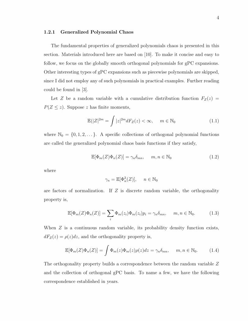
1.2.1 Generalized Polynomial Chaos

The fundamental properties of generalized polynomials chaos is presented in this

section. Materials introduced here are based on [10]. To make it concise and easy to

follow, we focus on the globally smooth orthogonal polynomials for gPC expansions.

Other interesting types of gPC expansions such as piecewise polynomials are skipped,

since I did not employ any of such polynomials in practical examples. Further reading

could be found in [3].

Let Z be a random variable with a cumulative distribution function FZ(z) =

P (Z z). Suppose z has finite moments,

E(|Z|2m =

Z|z|2mdFZ(z) <1, m 2 N0 (1.1)

where N0 = {0, 1, 2, . . . }. A specific collections of orthogonal polynomial functions

are called the generalized polynomial chaos basis functions if they satisfy,

E[�m(Z)�n(Z)] = �n�mn, m, n 2 N0 (1.2)

where

�n = E[�2n(Z)], n 2 N0

are factors of normalization. If Z is discrete random variable, the orthogonality

property is,

E[�m(Z)�n(Z)] =X

i

�m(zi)�m(zi)pi = �n�mn, m, n 2 N0. (1.3)

When Z is a continuous random variable, its probability density function exists,

dFZ(z) = ⇢(z)dz, and the orthogonality property is,

E[�m(Z)�n(Z)] =

Z�m(z)�m(z)⇢(z)dz = �n�mn, m, n 2 N0. (1.4)

The orthogonality property builds a correspondence between the random variable Z

and the collection of orthogonal gPC basis. To name a few, we have the following

correspondence established in years.

5

• Standard Gaussian random variable Z ⇠ N(0, 1) — Hermite polymonials

• Uniformly distributed random variable Z ⇠ U(�1, 1) — Legendre polymonials

• Beta distributed random variable Z ⇠ B(�1, 1) — Jacobi polymonials

• Gamma distributed random variable Z ⇠ �(k+1, 1, 0) — Laguerre polymonials

Refer to Table 5.1 in [10] for details of other commonly used distributions.

To define similar polynomial expansions for multiple random variables, we only

have to employ multivatiate gPC expansion. Let Z = (Z1, Z2, . . . , Zd) be a random

vector with CDF FZ(z1, z2, . . . , zd), where all Zi’s are mutually independent. There-

fore, FZ(z) =Qd

i=1 FZi(zi). Let {�k(Zi)}Nk=0 2 PN(Zi) be the univariate gPC basis

functions in the variable Zi with degree up to N , i.e,

E[�m(Zi)�n(Zi)] =

Z�m(z)�m(z)dFZi(z) = �n�mn, 0 m,n N. (1.5)

Let i = (i1, i2, . . . , id) 2 Nd0 be a multi index with |i| = i1 + i2,+ · · · + id. The

multivatiate gPC basis functions with N degree are the product of univariate gPC

polynomials with total degree being les than or equal to N , that is,

�i(Z) = �i1(Z1) · · ·�id(Zd), 0 |i| N. (1.6)

Thus, the following holds,

E[�i(Z),�j(Z)] =

Z�i(z),�j(z)dFZ(z) = �i�ij (1.7)

where �i = E[�2i ] = �i1 · · · �id are the factors of normalization and �ij = �i1ji · · · �idjd is

the d-variate Kronecker delta function. These polynomials span PdN with dimension

dim PdN =

✓N + d

N

◆, (1.8)

which is the linear space of all polynomials of degree less than or equal to N with

d variabls. When we apply classical approximation theory to any mean-square inte-

grable functions of Z with respect to the measure dFZ , we can have some conclusion

as

||f � PNf ||L2dFZ! 0, N !1 (1.9)

6

where PN is the orthogonal projection operator. It is obvious that the dimension is

still increasing too fast with respect to d and N . The curse of dimensionality is there

proventing us from getting high accuracy in approximation with high dimensional

random variables Z. This is exactly what my localized strategy is going to avoid,

which will help reduce computation cost in a large scale. I pause here with enough

discussion of gPC expansion notations and issues. Then, I will dive into two commonly

used methods for solving stochastic systems in the next two sections.

1.2.2 Stochastic Galerkin Method

In this section, I present the framework of the generalized polynomial chaos

Galerkin method for solving stochastic systems such as stochastic partial di↵eren-

tial equations (sPDE).

Without loss of generality, for a physical domain D ⇢ Rl, l = 1, 2, 3, and T > 0,

the a stochastic PDE system could be represented as following,8>>><

>>>:

ut(x, t, Z) = L(u), D ⇥ (0, T ]⇥ Rd,

B(u) = 0, @D ⇥ [0, T ]⇥ Rd,

u = u0, D ⇥ [t = 0]⇥ Rd,

(1.10)

where L is the di↵erential operator, B is the boundary condition operator and u0 is

the initial condition. Z = (Z1, Z2, . . . , Zd) 2 Rd, d � 1, are mutually independent

random variables featuring the random inputs of the equation system. Consider a

simple representation of u as scaler function, i.e,

u(x, t, Z) : D ⇥ [0, T ]⇥ Rd R, (1.11)

we will apply apply gPC expansion to each existence of u. As discussed in the gPC

basic notations, {�k(Z)} is the set of gPC basis functions satisfying

E[�i(Z),�j(Z)] = �i�ij. (1.12)

7

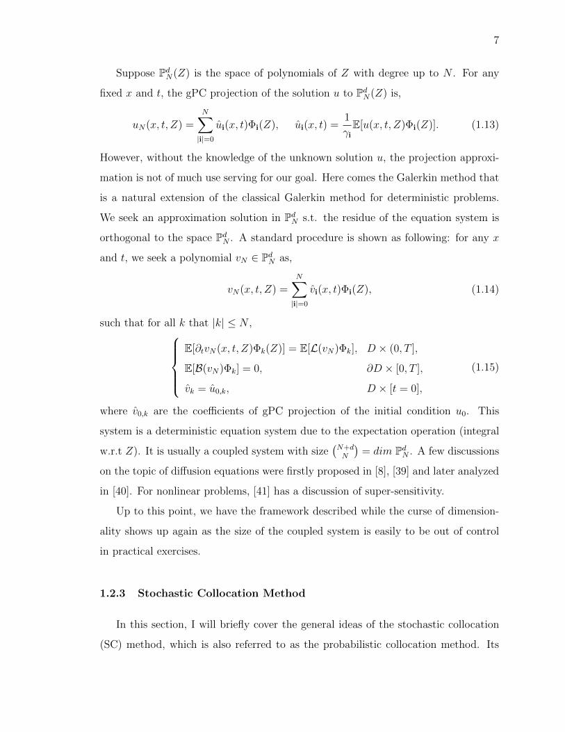
Suppose PdN(Z) is the space of polynomials of Z with degree up to N . For any

fixed x and t, the gPC projection of the solution u to PdN(Z) is,

uN(x, t, Z) =NX

|i|=0

ui(x, t)�i(Z), ui(x, t) =1

�iE[u(x, t, Z)�i(Z)]. (1.13)

However, without the knowledge of the unknown solution u, the projection approxi-

mation is not of much use serving for our goal. Here comes the Galerkin method that

is a natural extension of the classical Galerkin method for deterministic problems.

We seek an approximation solution in PdN s.t. the residue of the equation system is

orthogonal to the space PdN . A standard procedure is shown as following: for any x

and t, we seek a polynomial vN 2 PdN as,

vN(x, t, Z) =NX

|i|=0

vi(x, t)�i(Z), (1.14)

such that for all k that |k| N ,8>>><

>>>:

E[@tvN(x, t, Z)�k(Z)] = E[L(vN)�k], D ⇥ (0, T ],

E[B(vN)�k] = 0, @D ⇥ [0, T ],

vk = u0,k, D ⇥ [t = 0],

(1.15)

where v0,k are the coe�cients of gPC projection of the initial condition u0. This

system is a deterministic equation system due to the expectation operation (integral

w.r.t Z). It is usually a coupled system with size�N+dN

�= dim Pd

N . A few discussions

on the topic of di↵usion equations were firstly proposed in [8], [39] and later analyzed

in [40]. For nonlinear problems, [41] has a discussion of super-sensitivity.

Up to this point, we have the framework described while the curse of dimension-

ality shows up again as the size of the coupled system is easily to be out of control

in practical exercises.

1.2.3 Stochastic Collocation Method

In this section, I will briefly cover the general ideas of the stochastic collocation

(SC) method, which is also referred to as the probabilistic collocation method. Its

8

systematic introduction could be found in [42]. A few notations of SC method will

be introduced and two major numerical interpolation approaches will be discussed,

i.e, Tensor Product Collocation and Sparse Grid Collocation.

Collocation method, unlike the Galerkin method, requires the residue of the gov-

erning system equations to be zero on prescribed nodes in the domain. These nodes

are also called collocation points, which is widely studied in the deterministic nu-

merical analysis. Take the same sPDE system as it in Galerkin method section as

example,

8>>><

>>>:

ut(x, t, Z) = L(u), D ⇥ (0, T ]⇥ Rd,

B(u) = 0, @D ⇥ [0, T ]⇥ Rd,

u = u0, D ⇥ [t = 0]⇥ Rd,

(1.16)

where d � 1. Assume w(·, Z) is a numerical approximation to the actual solution

u for a fixed x and t. Obviously 1.16 cannot be satisfied over all Z when using the

approximation solution w. But we can make them exact on a collection of points.

Let ⇥M = {Z(j)}Mj=1 ⇢ IZ be a collection of prescribed nodes in the random space,

where IZ is the support of Z and M 1 is the total number of nodes. Then, by

enforcing the following deterministic system, we have the collocation method formu-

lation, for j = 1, 2, . . . ,M8>>><

>>>:

ut(x, t, Z(j)) = L(u), D ⇥ (0, T ],

B(u) = 0, @D ⇥ [0, T ],

u = u0, D ⇥ [t = 0].

(1.17)

As long as the original problem has a well-defined deterministic algorithm, the col-

location system showed above could be easily solved for each j. Assume we have

the solution to the above problems, namely u(j) = u(·, Z(j)), j = 1, 2, . . . ,M . We

can employ a variety of numerical methods to do the post-processing of u(j)’s to (ap-

proximately) obtain any kind of detailed information of the exact solution u(Z). A

straight forward example is Monte Carlo sampling method, which randomly gener-

ate sample points Z(j) depending on the distribution of Z. Another good example

9

is deterministic sampling method, which usually use nodes of quadrature rules in

multi-dimensions. The convergence of these methods is usually based on the solution

statistics, i.e, mean, variance, moments, which is in the sense of weak convergence.

In the following paragraphs, I will go over the framework of interpolation approach

which will give the convergence in the sense of strong convergence (Lp norm).

It is natural to adopt interpolation approach to stochastic collocation problem by

letting the approximating solution w be exact on a collection of nodes. Therefore,

given the nodal set ⇥M ⇢ |Z and {u(j)}Mj=1, we seek a polynomial w(Z) in a proper

polynomial space ⇧(Z) such that w(Z(j)) = u(j) for all j = 1, 2, . . . ,M .

The Lagrange interpolation is one straightforward approach for that goal,

w(Z) =MX

j=1

u(Z(j))Lj(Z), (1.18)

where

Lj(Z(k))) = �jk, 1 j, k M, (1.19)

It is easy to implement Lagrange interpolation, but the trade o↵ is that many funda-

mental issues of Lagrange interpolation with high dimension (d � 1) are not clear.

Another approach is to adopt the matrix inversion method. We will pre-decide

the polynomial basis for the interpolation, e.g., we choose the collection of gPC basis

�k(Z) and naturally build the approximation function as,

wN(Z) =NX

|k|=0

wk�k(Z). (1.20)

where wk’s are the unknown coe�cients. Then, we apply the interpolation condition

w(Z(j)) = u(j) for j = 1, 2, . . . ,M , which gives,

AT w = u (1.21)

where

A = (�k(Z(j))), 0 |k| N, 1 j M, (1.22)

is the coe�cient matrix, u = (u(Z(1)), u(Z(2)), . . . , u(Z(M)))T and w is the unknown

vector of coe�cients. It is obvious that we have to make sure M ��N+dN

�such that

10

the system is not under-determined. On one side, it is good to use matrix inversion

method, since nodal set is given and we can guarantee the existence of interpolation

by examining A and its determinant. On the other hand, issues and concerns are still

there with accuracy of the approximation. Zero interpolation errors on nodes does not

guarantee a good approximation result in the place between nodes, it is particularly

true in multidimensional cases. Though, we know that using nodes that are zeros of

the orthogonal polynomials {�k(Z)} will o↵er relatively high accuracy, there is still

no universal approaches that would provide satisfactory for general purposes, but we

can still find a few good candidates.

Tensor Product Collocation

It is natural to consider employing a univariate interpolation and fill the entire

space on each single dimension, which brings up the Tensor Product Collocation ap-

proach. By doing so, most of the error analysis and nice features would be maintained

in the multi-variate interpolation.

For any 1 i d, let Qmi be the interpolating operator such that,

Qmi [f ] = umif(Zi) 2 Pmi(Zi) (1.23)

is an interpolating polynomial of degree mi, for a given function f in the Zi variable.

It used mi +1 nodes, namely ⇥mi1 = {Z(1)

i , ..., Z(mi+1)i }. Then, to interpolate f in the

entire space IZ ⇢ Rd is to use the tensor product of interpolating operators,

QM = Qm1 ⌦ · · ·⌦Qmd(1.24)

where the collection of nodes is,

⇥M = ⇥m11 ⇥ · · ·⇥⇥md

1 (1.25)

and M = m1 ⇥ · · · ⇥ md. Most of the properties of the 1D interpolation approach

are retained when we adopt the tensor product collocation method. Error analysis

for the entire space could be derived from the 1D error bound. To simplify the

11

argument, we assume the number of nodes in each dimension stay the same, i.e.,

m1 = m2 = · · · = md = m, then the 1D interpolation error in the i-th dimension is,

(I �Qmi)[f ] / m�↵ (1.26)

where ↵ depends on the smoothness of the function f . The total interpolation error

follows,

(I �QM)[f ] /M�↵/d, d � 1, (1.27)

where we substitute m by M1/d. This is an unfortunate situation for convergence,

since the convergence rate decreases rapidly when d!1. Additionally, the size of the

collection of nodes is large M = md. For large d, it is something that we cannot(don

not want) to a↵ord in computation, since each collocation node will require to solve

the deterministic governing problem once in whatever numerical approach you choose.

This brings up the curse of dimensionality again and could only be accepted with low

dimensional PDE systems (It works well when d 5). See [43] for details about

stochastic di↵usion equations.

Sparse Grid Collocation

Using Smolyak sparse grid is another (better) approach compared to tensor prod-

uct approach. It is firstly proposed in [44], and is studied by many researchers recently.

To briefly present its core idea, it is important to know that Smolyak sparse grids are

just a (proper) subset of the full tensor grids. It can be constructed by the following

form (given in [45]),

QN =X

N�d+1|i|N

(�1)N�|i| ·✓

d� 1

N � |i|

◆· (Qi1 ⌦ · · ·⌦Qid) (1.28)

where N � d is the level of the construction. 1.28 confirms that Smolyak sparse grid

is a combination of subsets of tensor product grids. The chosen nodes are,

⇥M =[

N�d+1|i|N

(⇥i11 ⇥ · · ·⇥⇥id

1 ) (1.29)

12

It is hard to give a close form of number of nodes in ⇥M in term of M and N .

It is interesting and helpful if we decides to let 1D nodal sets be nested, which is

given by the following definition,

⇥i1 ⇢ ⇥j

1, i < j. (1.30)

Studies show that the total number of nodes in 1.29 is minimized when we have the

nested nodal sets. Bad news is that if we adopt the nodes as zeros of orthogonal

polynomials, we will not have such a nice nesting property.

We can turn to a popular choice of Clenshaw-Curtis nodes, which are the extrema

of the well-known Chebyshev polynomials, for a given integer i in the range [1, d],

Z(j)i = � cos

⇡(j � 1)

mki � 1

, j = 1, 2, . . . ,mki (1.31)

where we use k to index the node set with di↵erent size in the nested manner. With

increasing index k, the size of node set is almost doubled for each increment on k,

i.e., mki = 2k�1 + 1, and the conner case is defined as m1

i = 1 and Z(1) = 0. It is

easy to verify the nesting property for this setting. And we denote the index k as the

level of Clenshaw-Curtis grids. It is obvious that the larger k is, the finer the grids.

See [46] for details.

Though there is no explicit closed form for the total number of nodes in the nodal

set, we have a rough estimate of that amount as following,

M = |⇥k| ⇠2kdk

k!, d� 1. (1.32)

Studies has be done in [47] that the Clenshaw-Curtis sparse grid interpolation gives

exact representation of functions in Pdk. When d � 1, we have dim Pd

k =�d+kd

�⇠

dk/k!. Therefore, to accurately represent a function in Pdk, we need approximately a

2k multiplicative constant, which is irrelevant to dimension d. A fundamental result

in [47] gives a boundary of the approximation error.

Theorem 1.2.1 For functions in space F ld = {f : [�1, 1]d ! R|@|i|fcontinuous, ik

l, 8k}, the interpolation error is bounded by,

||I �QM ||1 Cd,lM�l(logM)(l+2)(d�1)+1

13

This error estimation shows a little bit better bound, but still su↵ers from the curse

of dimensionality when d is getting larger and larger. However, the reduction in the

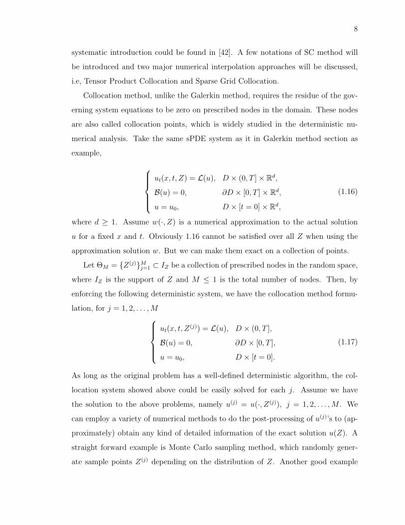
size of nodal set could be well observerd as shown in Figure 1.1

Figure 1.1. 2-dimensional interpolation grids based on Clenshaw-Curtis nodes (1-dimensional extrema of Chebyshev polynomials) atlevel k = 5. Left: tensor product grids. Right: Smolyak sparse grids.

1.3 Research Outline

With the basic tools introduced in the previous sections, we can dive into de-

tails of a numerical method that solves stochastic partial di↵erential equations with

a local solver and a global coupling strategy. The primary methodology/routine is

introduced in Chapter 2 with general cases and a detailed example for di↵usion equa-

tions. The method is designed not to be limited in a specific type of equations, but

a good example will make reader easily understand how it works and what to expect

in details. In Chapter 3, a brief error analysis and discussion is proposed and exam-

ined. To further validate the methodology and build connections/relationships with

local strategy for deterministic problems, I provide the Chapter 4 as a guide to the

comparision with the Steklov-Poincare interface equation and the classical Schur com-

plement. A variety of numerical examples including 1D and 2D di↵usion equations

and a multiphysics example are presented in Chapter 5.

14

The text of this dissertation includes some reprints of the the following papers,

either accepted or submitted for consideraton at the point of publication. The dis-

sertation author was the author of these publicatons.

Y. Chen, X. Zhu, and D. Xiu, Properties of Local Polynomial Chaos Expansion

for Linear Di↵erential Equations, 2016.

Y. Chen, J. Jakeman, C. Gittelson and D. Xiu, Local Polynomial Chaos Expansion

for Linear Di↵erential Equations with High Dimensional Random Inputs, SIAM J. Sci.

Comput., 2014. 37(1), A79A102.

15

2. LOCALIZED POLYNOMIAL CHAOS METHODOLOGY

2.1 Problem Setup

Consider the following setting of a partial di↵erential equation with random in-

puts. Let D ⇢ R`, ` = 1, 2, 3, be a physical domain with boundary @D and coordi-

nates x = (x1, . . . , x`) 2 D. Let ⌦ be the event space in a properly defined probability

space. Consider the following SPDE:8<

:L(x, u; a(x,!)) = f(x), in D ⇥ ⌦,

B(x, u; a(x,!)) = 0, on @D ⇥ ⌦,(2.1)

where L is a di↵erential operator, B is a boundary operator. The random input

a(x,!) is a random process on the physical domain, i.e.,

a(x,!) : D ⇥ ⌦! R.

We make a fundamental assumption that the governing equation (2.1) is well posted

almost everywhere in the probability space ⌦. For simplicity of notation and without

loss of generality, we assume f(x) is deterministic.

2.1.1 PDE with Random Inputs

For the practical purpose, the random input usually needs to be parameterized

by a set of random variables. The parametrization usually employs a linear form of

a set of random variables, e.g.,

a(x,!) ⇡ a(x, Z) = µa(x) +dX

i=1

↵i(x)Zi(!), (2.2)

where µa(x), {↵i(x)} and {Zi} are the mean, spatial functions and random variables,

respectively. A widely used method of the parametrization process is the so called

16

Karhunen-Loeve (KL) expansion. Given a covariance function C(x, y) of the random

process a(x,!), where

C(x, y) = E[(a(x,!)� µa)(a(y,!)� µa(y))], (2.3)

The Karhunen-Loeve (KL) expansion gives the parametrization, i.e.,

a(x,!) ⇡ aKL(x, Z) = µa(x) +dX

i=1

p�i i(x)Zi(!), (2.4)

where {�i, i(x)} are the eigenvalues and eigenfunctions of the covariance function

such that,

Z

D

C(x, y) i(x)dx = �i i(y), i = 1, 2, 3, . . . , x, y 2 D, (2.5)

and the random vector Z = (Z1, Z2, Z3, . . . , ) are defined as follows,

Zi(!) =1p�i

Z

D

(a(x,!)� µa(x)) i(x)dx, i = 1, 2, 3, . . . , (2.6)

These random variables Z1, Z2, Z3, . . . , statisfy E[Zi] = 0 and E[ZiZj] = 0 by a simple

derivation of there definitions.

With the non-increasing ordering of eigenvalues in (2.5), one can usually truncate

the expansion in a finite number d as the eigenvalue decays to a su�ciently small

value. In fact, the decay rate of the eigenvalues depends on the correlation length of

covariance function C(x, y). Typically, the longer the correlation length, the faster the

decay and the smoother the random curve is, and vice versa. Therefore, a finite-term

series in the form of (2.2) is established in (2.4).

Upon such a parameterization of the global input a(x,!), the original SPDE (2.1)

is transformed into the following finite-dimensional problem with Z 2 Iz ⇢ Rd,8<

:L(x, u; a(x, Z)) = f(x), in D ⇥ ⌦,

B(x, u; a(x, Z)) = 0, on @D ⇥ ⌦,(2.7)

As mentioned earlier, when the input a(x,!) has short correlation length, the

parameterized global inputs aKL(x, Z) will have a larger number of terms. A slow

17

decay of the eigenvalues in KL expansion in (2.5) is observed by tons of experiments.

Consequently, the resulting high dimensional random space Z 2 Rd, d� 1 makes the

problem very time consuming to solve, as most of the existing numerical methods,

e.g., stochastic Galerkin methods, stochastic collocation methods, su↵er from the

curse-of-dimensionality. Our goal is to propose a methodology to address this well

known issue and tackle this computational challenge.

Though Karhunen-Loeve expansion (2.4) is employed in the exposition of our

method hereafter, we confirm that other types of input parameterization methods, in

the form of (2.2), can be readily used. The following methodology we present applies

equally well to other parameterization methods. It is always true that global input

of random processes with short correlation length results in high dimensional random

space, regardless of the exact form of the parameterization.

2.1.2 Domain Partitioning

Following our natural instinct, we decompose the spatial domain D into K non-

overlapping subdomains D(i), i = 1, . . . , K, such that,

D =K[

i=1

D(i), D(i) \D(j) = ;, j 6= i. (2.8)

and the partition is geometrically conforming, i.e., the intersection between two clo-

sure of any two subdomains is either an entire edge, a vertex or empty.

The traditional deterministic domain decomposition method (DDM) always em-

ploy a specific coupling conditions as the subdomain interfaces. We will adopt a

similar approach on the interface. We assume that the original problem (2.1) can be

solved in each subdomain with proper coupling conditions at the interfaces. In fact,

under a suitable regularity assumption (e.g. f us square-summable and the bound-

aries of subdomains are Lipschitz [48]), the original problem (2.1) is equivalent to the

18

following local problem on each subdomain with proper coupling conditions. More

specifically, for each i = 1, . . . , K, let8>>><

>>>:

L(x, u(i); a(x,!)) = f(x), in D(i),

C(ij)(x, u(j); a(x,!)) = 0, on @D(i) \ @D(j), j 6= i,

B(x, u(i); a(x,!)) = 0, on @D(i) \ @D,

(2.9)

where C(ij) stands for the coupling operator between neighboring subdomainsD(i) and

D(j). Then the global solution of the original problem can be naturally represented

in the following form,

u(x,!) =KX

i=1

u(i)(x,!)ID(i)(x), (2.10)

where IA is the indicator function satisfying

IA(x) =

8<

:1, x 2 A,

0, x /2 A.(2.11)

Note that this is quite a mild assumption on the governing equation (2.1). The

coupling operator C(ij) we refer to in (2.9) is exactly the coupling operator that is

widely used in traditional deterministic domain decomposition method. The specifi-

cation of the coupling operator C(ij) obviously depends on the problem.

2.1.3 Definition of Subdomain Problem

We make another fundamental assumption that each local problem (2.9) can be

well defined and be solved independently with a proper prescription of boundary

condition on the interface �(i). Suitable boundary conditions to ensure the solvability

vary and depend on the type and nature of the underlining PDE model. For example,

for a large class of PDEs, it is enough to impose Dirichlet boundary data to guarantee

the well-posedness of the problem. That is, for each i = 1, ..., K,8<

:L(x, w(i); a(x,!)) = f(x), in D(i),

w(i) = �(i)(x,!), on �(i) ⇢ @D(i),(2.12)

19

is well defined problem with proper boundary data �(i). Note that at this step,

each subdomain problem is independent of each other and bear no relation with the

solution of the original global problem (2.1), because they are uncoupled and satisfy

any Dirichlet boundary conditions. We tend to move the coupling process to later

stage to make our subdomain solver parallel or even reduced to a single subdomain

for some cases. It is also approved to apply any other type of boundary conditions to

make the subdomain problem independently solvable. We will continue our discussion

with the setup in (2.12)

2.2 Methodology

Given a specific domain partitioning stretagy, the general idea behind our local

polynomial chaos expansion is to solve independent sumdomain problems with arti-

ficial boundary conditions, e.g., the Derichlet conditions in (2.12). The idea relies

on the nature that we do not explicitly specify boundary conditions as deterministic

input values. Instead, we treat them as auxiliary variables or the so called unknown

parameters. We then seek a collection of numerical solutions of all existing equation

systems in (2.12) for i = 1, ..., K, that have functional dependence on input random

variables and auxiliary boundary variables. In the later stage, we sample the input

random variables and the couple local solutions under proper conditions to ensure a

global solution that satisfies the global problem (2.1).

2.2.1 Local Parameterization of Subdomain Problems

Though (2.1) is a localized version of the global problem (2.1), we still have to

make a parameterization to process the random input term a(x,!) in each subdomain

D(i). It is also necessary to parametrize the boundary condition �(i) locally. Due to

the distinct nature of these two type of variables(parameters), in each subdomain

D(i), we adopt di↵erent stretagy for them, i.e., local KL expansion for random input

20

parameters and numerical discretization in physical space for boundary condition

parameters.

Local KL Expansion

Recall the discussion in global parametrization of random input a(x,!), the decay

rate of the eigenvalues depends critically on the relative correlation length of the

process. This is the key to achieve the goal that we approximate local random input

with fewer required random parameters in each subdomain. A detailed workthrough

and is given in the following discussion.

In each subdomain i = 1, . . . , K, let

a(i) = a(x,!)ID(i)(x). (2.13)

be the input process in each subdomainD(i). We denotes the mean of random input in

each subdomain as µ(i)a (x) = µa(x)ID(i)(x) in the same manner. The covariance func-

tion C(x, y) stay the same. Then the corresponding KL expansion can be obtained

as follows,

a(i)(x,!) ⇡ a(i)(x, Z(i)) = µ(i)a (x) +

d(i)X

j=1

q�(i)j

(i)j (x)Z(i)

j (x), (2.14)

where {�(i)j , ij} are the local eigenvalues and eigenvalues of

Z

D(i)

C(x, y) (i)j (x)dx = �(i)j

(i)j (y), j = 1, . . . , d(i), x, y 2 D(i), (2.15)

and the local random random variables Z(i) = (Z(i)1 , . . . , Z(i)

d(i)) are defined as follows:

Z(i)j (!) =

1q�(i)j

Z

D(i)

(a(i)(x,!)� µ(i)a (x)) (i)

j (x)dx, j = 1, . . . , d(i). (2.16)

We have done a similar trunction at d(i) as it in the global KL expansion according

to any necessary accuracy requirement. To make it distinguishable from the global

KL expansion of random input a(x,!), we use a superscript (i) for subdomain D(i).

21

The decay rate of eigenvalues �(i)j depends critically on the relative correlation length,

which has been shrinked by the domain partitioning process as we designed. That is,

for a given random process a(x,!) with a correlation length à in a physical domain

E, it is its the relative correlation length

à,E / à/È, (2.17)

where È scales as the diameter of the domain E, that determines the eigenvalue decay

rate. The longer the relative correlation length the faster the decay of the eigenvalues,

and vice versa. It is now obvious that, with the domain partitioning process, we

are able to make the size of each subdomain small enough to generate a relatively

reasonable correlation length for a parametrization of a reasonable (relativelly small)

number of random parameters, i.e., making di ⌧ d in (2.14).

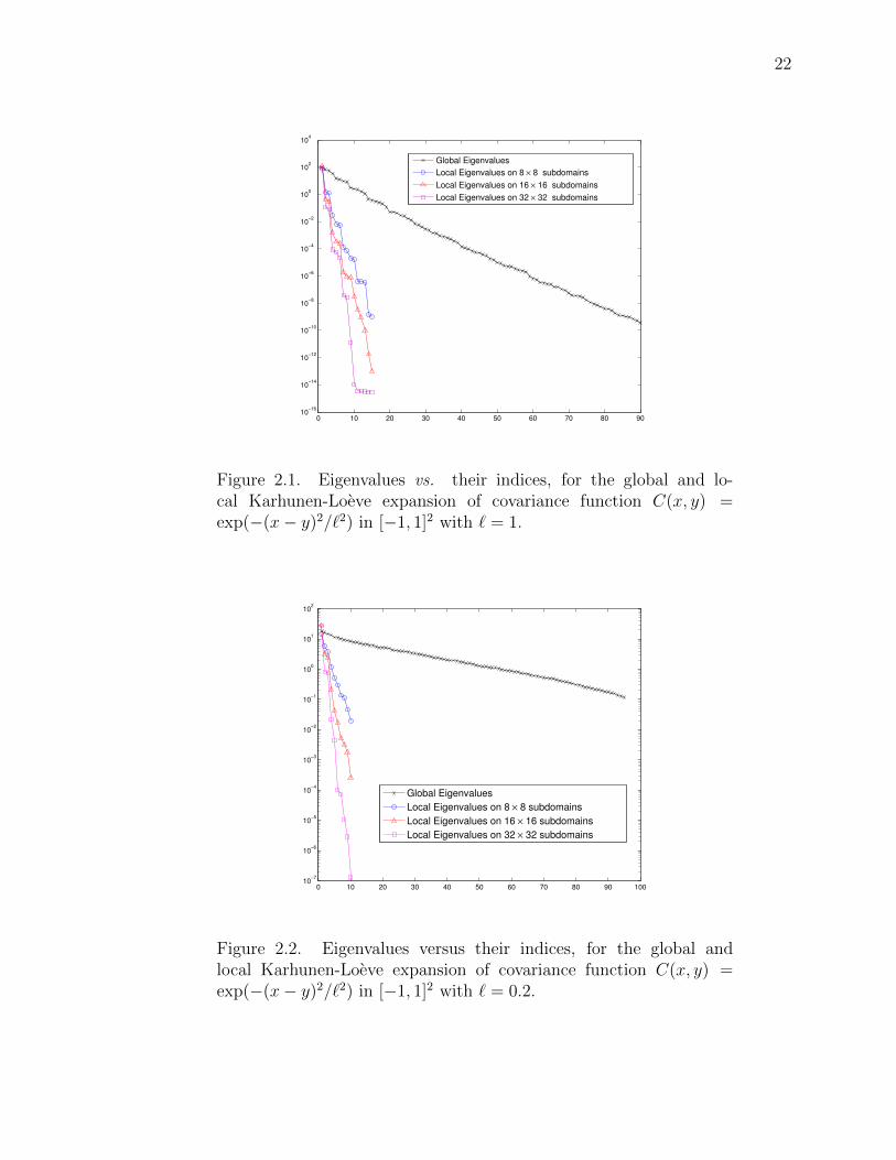
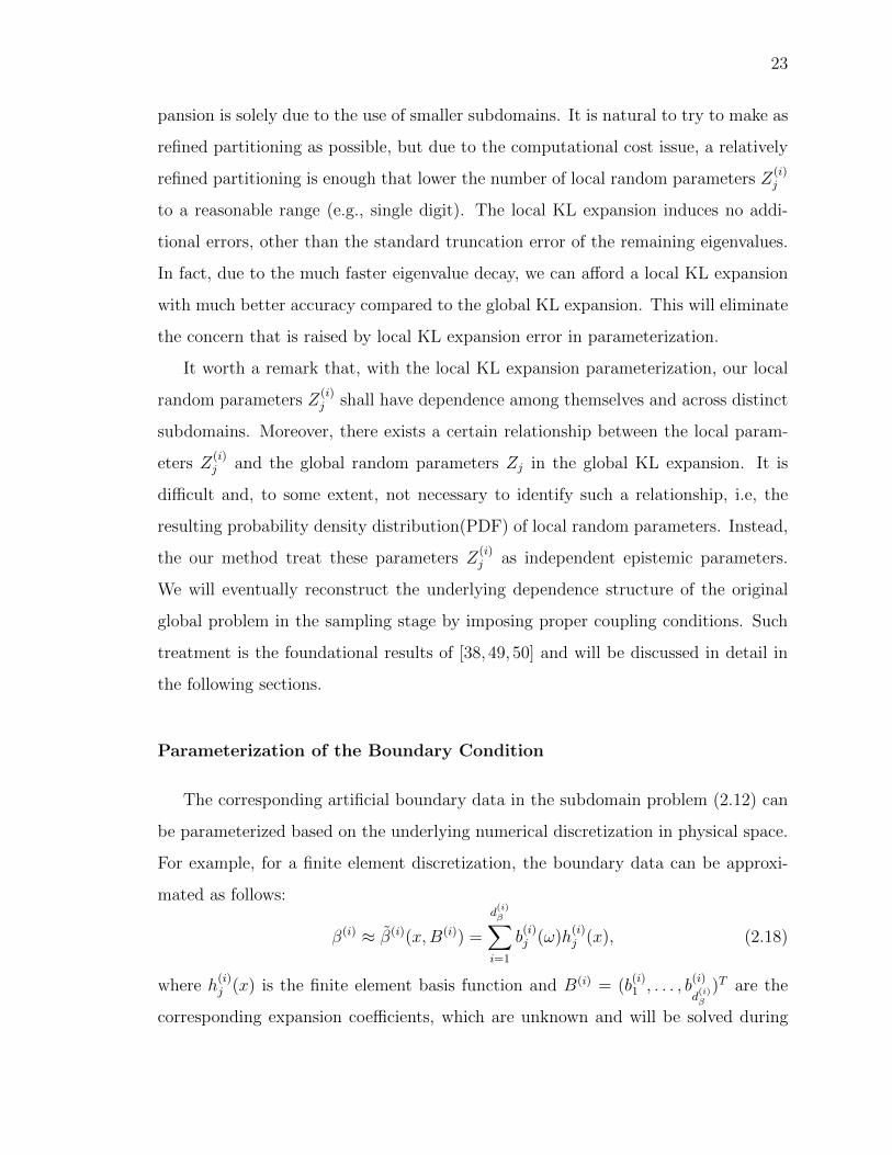
This fact has been discovered and studied by a number of researchers. Here

we present a nice demonstration of eigenvalue decay of KL expansion in a two-

dimensional square domain D = [�1, 1]2 for a Gaussian random process with co-

variance function C(x, y) = exp(�(x � y)2/`2) with a fixed correlation length `. In

Figure 2.1, the correlation length is set as ` = 1. We show the eigenvalues of the

global KL expansion and eigenvalues of the local KL expansions with domain par-

titioning as (8 ⇥ 8), (16 ⇥ 16), and (32 ⇥ 32) square subdomains. A mach faster

eigenvalue decay pattern is observed in local KL expansion compared to the global

KL expansion. For example, to keep a certain level of total spectrum (about 95%),

the global KL requires d = 25 ⇠ 30 terms, whereas the (8 ⇥ 8) partitioning requires

only d(i) = 4 terms and the (32 ⇥ 32) partitioning only requires d(i) = 3 terms. In

Figure 2.2, a similar result is shown for the correlation length ` = 0.2. For this rela-

tive short correlation length, the eigenvalues of the global KL expansion decay much

slowly. It requires around d = 70 ⇠ 90 terms to capture about 95% of the spectrum.

On the other hand, the local KL expansion still only requires a much smaller number

of terms, i.e., around d(i0) = 5 on (8⇥ 8) partitioning and d(i) = 3 on (32⇥ 32) par-

titioning. The reduction in random input dimensionality is significant through these

demonstrations. The drastic reduction in random dimensionality by the local KL ex-

22

0 10 20 30 40 50 60 70 80 9010

−16

10−14

10−12

10−10

10−8

10−6

10−4

10−2

100

102

104

Global Eigenvalues

Local Eigenvalues on 8 × 8 subdomains



Figure 2.1. Eigenvalues vs. their indices, for the global and lo-cal Karhunen-Loeve expansion of covariance function C(x, y) =exp(�(x� y)2/`2) in [�1, 1]2 with ` = 1.

0 10 20 30 40 50 60 70 80 90 10010

−7

10−6

10−5

10−4

10−3

10−2

10−1

100

101

102

Global Eigenvalues




Figure 2.2. Eigenvalues versus their indices, for the global andlocal Karhunen-Loeve expansion of covariance function C(x, y) =exp(�(x� y)2/`2) in [�1, 1]2 with ` = 0.2.

23

pansion is solely due to the use of smaller subdomains. It is natural to try to make as

refined partitioning as possible, but due to the computational cost issue, a relatively

refined partitioning is enough that lower the number of local random parameters Z(i)j

to a reasonable range (e.g., single digit). The local KL expansion induces no addi-

tional errors, other than the standard truncation error of the remaining eigenvalues.

In fact, due to the much faster eigenvalue decay, we can a↵ord a local KL expansion

with much better accuracy compared to the global KL expansion. This will eliminate

the concern that is raised by local KL expansion error in parameterization.

It worth a remark that, with the local KL expansion parameterization, our local

random parameters Z(i)j shall have dependence among themselves and across distinct

subdomains. Moreover, there exists a certain relationship between the local param-

eters Z(i)j and the global random parameters Zj in the global KL expansion. It is

di�cult and, to some extent, not necessary to identify such a relationship, i.e, the

resulting probability density distribution(PDF) of local random parameters. Instead,

the our method treat these parameters Z(i)j as independent epistemic parameters.

We will eventually reconstruct the underlying dependence structure of the original

global problem in the sampling stage by imposing proper coupling conditions. Such

treatment is the foundational results of [38, 49, 50] and will be discussed in detail in

the following sections.

Parameterization of the Boundary Condition

The corresponding artificial boundary data in the subdomain problem (2.12) can

be parameterized based on the underlying numerical discretization in physical space.

For example, for a finite element discretization, the boundary data can be approxi-

mated as follows:

�(i) ⇡ �(i)(x,B(i)) =

d(i)�X

i=1

b(i)j (!)h(i)j (x), (2.18)

where h(i)j (x) is the finite element basis function and B(i) = (b(i)1 , . . . , b(i)

d(i)�

)T are the

corresponding expansion coe�cients, which are unknown and will be solved during

24

the coupling stage later on. Note that if h(i)j (x) is a nodal finite element basis, b(i)j

represents the exact nodal value at the boundary, which could be random.

2.2.2 Solutions of the Subdomain Problems

With the local parameterization, the subdomain problem (2.12) can be reformu-

lated as follows: for each i = 1, . . . , K,8<

:L(x, w(i); a(i)(x, Z(i)) = f(x), in D(i),

w(i) = �(i)(x,B(i)), on �(i) ⇢ @D(i).(2.19)

Now, the solution depends on both local random parameters Z(i) ✓ Rd(i) and the

boundary parameters B(i) ✓ Rd(i)� . We take range of these random parameters into

consideration. Let the ranges be I(i)Z ✓ Rd(i) and I(i)B ✓ Rd(i)� , we have the following

description of our local solution,

w(i)(x, Z(i), B(i)) : D(i) ⇥ I(i)Z ⇥ I(i)B ! R. (2.20)

For this general scenario, the solution w(i) resides in a d(i) = (d(i) + d(i)� )-dimensional

space in addition to the physical domain.

General Procedure

The probability distributions for Z(i) and B(i) are unknown. But we have the

following numerical method developed in [51, 52] to take care of this kind of issue.

Here, we briefly review a few key steps.

First, we define the following random parameters to wrap up both Z(i) and B(i),

Y (i) = (Z(i), B(i)) 2 Red(i) , ed(i) = d(i) + d(i)� , (2.21)

with its range I(i)Y ✓ Red(i) . We then focus on the solution dependence in the param-

eter space, I(i)Y . We emphasize that the precise knowledge of the range I(i)Y and its

associated probability measure ⇢y is not available, which is, in fact, hard to obtain

25

and requires high computational cost. The method developed in [51, 52] proposes a

way to find a strong approximation of the solution in an estimated domain I(i)X , which

is a tensor-product domain that encapsulates the real domain I(i)Y in each dimension.

We impose the following restriction on it,

Prob(I(i)X 4I(i)Y ) �, � � 0, (2.22)

where 4 is the symmetric di↵erence operator between two sets and � should be a

small real number. Note that � can be zero if I(i)X is su�ciently large to completely

encapsulate I(i)Y .

It was shown that, if a strong approximation w(i) in I(i)X , e.g., in a weighted LpW

norm, can be obtained such that, for any fixed x,

✏ =��w(i)(x, ·)� ew(i)(x, ·)

��LpW (I

(i)X )⌧ 1, p � 1, (2.23)

where W is a weight function specified in I(i)X , then, the approximation w(i) can be a

good approximation to ew(i) in the real domain I(i)Y with respect to the real probability

⇢y in the following sense, (Theorem 3.2, [52])

��w(i)(x, ·)� ew(i)(x, ·)��Lp⇢y (I

(i)Y ) C1✏+ C2�, (2.24)

where C1 and C2 are constants unrelated to w(i). Note that w(i) can be obtained by

a standard numerical method, e.g., a gPC expansion using the specified measure W ,

in the well defined tensor domain I(i)X .

One of the immediate results is that even though w(i) is obtained via the weight W

unrelated to the true distribution ⇢y, its samples can be used as good approximations

to the true samples of ew(i). This fact is the foundation of the local gPC method here.

Simplification for Linear Equations

It is always good to examine and utilize the linearity in any collection of PDEs that

could simplify the underlying problem to a certain form. We have been looking into

26

the advantage of linear dependence of local solutions onto its boundary parameters,

we present the following formulation of a simplified problem.

Assume the original governing equation (2.1) is linear. The linearity ensures that

the solution is linear in terms of the boundary parameters B(i). Therefore, instead of

solving (2.19) in the ed(i)-dimensional parameter space, with ed(i) = d(i)+d(i)� , it can be

solved (d(i)� + 1) times in the d(i)-dimensional space for Z(i) in the following manner.

Using the parameterization of the boundary condition (2.18), we define, for each

j = 1, . . . , d(i)� ,

8<

:L(x, ew(i)

j (x, Z(i));ea(i)(x, Z(i))) = 0, in D(i),

ew(i)j = h(i)

j (x), on �(i) ✓ @D(i).(2.25)

We also define8<

:L(x, ew(i)

0 (x, Z(i));ea(i)(x, Z(i))) = f(x), in D(i),

ew(i)0 = 0, on �(i) ✓ @D(i).

(2.26)

Then, upon denoting b(i)0 = 1, the solution of (2.19) is

ew(i)(x, Z(i), B(i)) =

d(i)�X

j=0

b(i)j ew(i)j (x, Z(i)). (2.27)

Problem (2.25) and (2.26) are standard stochastic problems in the subdomainD(i),

with its random input ea, parameterized via the local KL expansion of very low di-

mension d(i), and deterministic boundary condition h(i)j and zero respectively. We can

then apply a standard stochastic method, e.g., gPC Galerkin method or collocation

method, to solve the problem and obtain ew(i)j,N ⇡ ew

(i)j , for each j = 0, . . . , d(i)� .

Then, the approximate solution of (2.19) is

ew(i)N (x, Z(i), B(i)) =

d(i)�X

j=0

b(i)j ew(i)j,N(x, Z

(i)). (2.28)

We remark that the linear dependence of the boundary parameters B(i) is exact, due

to the linearity of the governing equation. On the other hand, the random parameters

27

Z(i) are from the input a(x,!), which one should have su�cient information to be

able to sample directly. Consequently, obtaining the solution (2.28) does not require

the explicit encapsulation step described in the previous section and the numerical

error from (2.24) will not contain the second term (i.e., � = 0). Hereafter, we will

continue to use the notations Z(i) and B(i) or their wraped version Y (i), instead of

evoking the encapsulation variable X(i).

Note that, we have utilized the linearity of an original global PDE to simplify the

formulation of local problem in this section. But we will continue our discussion for

general PDEs, not restricted in the linear family. We will continue to discuss the

general procedure of obtaining global solution by coupling local solutions, and it will

work for a general purpose, and is also a nice guideline for PDEs in linear family.

2.2.3 Global Solution via Sampling

To recover the global numerical solution for a given random vector Z,

wN =KX

i=1

d(i)�X

j=0

b(i)j w(i)N,j(x, Z

(i))ID(i) , (2.29)

we need to determine two sets of local parameters Z(i), B(i) by the coupling the subdo-

main problems. Here we present a sampling method to determine these parameters.

This involves two levels of coupling: (1) correct probabilistic structure of the solu-

tion is enforced through direct sampling of the local random variables Z(i) from a

realization of the global random input a(x, Z). (2) correct physical constraints of the

solution at the interface is enforced via the proper coupling conditions (2.9). We shall

discuss the two steps in detail as follows.

Let M � 1 be the number of input samples we are able to generate. We use

subscript k to denote the samples and for each k = 1, . . . ,M we seek,

( ewN(x))k ⇡ (u(x))k, (2.30)

where ( ewN(x))k and (u(x))k are the kth sample of the numerical solution (2.29) and

of the exact solution (2.1), respectively.

28

Sampling the Random Inputs

The first step is to sample the random input a(x,!) to the original problem (2.1).

This is a straightforward procedure because it is assumed that one should always

be able to sample the random inputs. Let (a(x))k, k = 1, . . . ,M , M � 1, be these

samples, and

(a(x))(i)k = (a(x))kID(i)(x), i = 1, . . . , K, (2.31)

be their restrictions in each subdomains. Then, for each sample and in each subdo-

main D(i), we apply (2.16) to obtain the samples of the random variables in the local

KL expansion (2.14), i.e.,⇣Z(i)

j

⌘

k=

1q�(i)j

Z

D(i)

⇣(a(x))(i)k � µ(i)

a (x)⌘ (i)j (x)dx, j = 1, . . . , d(i). (2.32)

Upon doing so, we obtain the deterministic sample values for the random vector

(Z(i))k = ((Z(i)1 )k, . . . , (Z

(i)

d(i))k), k = 1, . . . ,M , in each subdomain D(i). Note that is a

straightforward deterministic problem. It is essentially a problem of approximating a

given deterministic function (a(x))k locally in D(i) via a set of deterministic orthog-

onal basis { (i)j (x)}. (The eigenfunctions of the KL expansion are orthogonal in the

physical space.) Any suitable approximation methods can be readily used and the

continuity of (a(x))k at the interfaces (if present) can be built in as a constraint. In

our examples we used the constrained least squares method [53].

Interface Problem

After determining the random parameters Z(i) for each solution sample, the only

undetermined parameters in (2.29) are the boundary parametersB(i) = (b(i)1 , . . . , b(i)d(i)�

).

They can be determined by enforcing the proper boundary conditions and the cou-

pling conditions at the subdomain interfaces, as in (2.9). That is, for each sample

k = 1, . . . ,M , and i = 1, . . . , K, we enforce the following conditions,8<

:C(ij)(x, ( ew(i)

N )k, ( ew(j)N )k; (a)

(i)k , (a)(j)k ) = 0, on @D(i) \ @D(j), j 6= i,

B(x, ( ew(i)N )k; (a)

(i)k ) = 0, on @D(i) \ @D.

(2.33)

29

Note that this is a system of deterministic algebraic equations with unknown param-

eters (B(i))k. It is our assumption that these conditions induce a well defined system

so that (B(i))k can be solved. This in turn determines the sample realizations (ew(i)N )k

completely. And we can construct the sample realizations of the global solution now.

( ewN(x))k =KX

i=1

( ew(i)N (x))kID(i)(x), k = 1, . . . ,M. (2.34)

We emphasize that the assumption that the coupling conditions induce a set of

well defined system of algebraic equations for the boundary parameters is not strong.

In fact, this is precisely what is required in the traditional deterministic domain

decomposition methods. We shall illustrate this point in the Chapter of Validation.

31

3. ERROR ANALYSIS

A complete error analysis for the methodology is not possible without specifying the

governing equation. Since the purpose of this chapter is to provide a guideline for con-

ducting error analysis, we will look at all possible error issues in the methodology for

a large collection of PDEs, including the linear family. We also include a full Chapter

of further validation to introduce the similar underlying theorem for our methodology

compared to the domain decomposition method for deterministic problems, which in

return also provide a variety of error analysis tools and results. To begin with, we

examine all possible error contributions in our numerical procedure.

3.1 Error Contributions

Since the local gPC method produces solutions in term of sample realizations in

the form of (2.34), it is natural to adopt a discrete norm over the solution samples.

Again, let M � 1 be the number of samples, for a collection of function samples

(f(x)) = ((f(x))1, . . . , (f(x))M) we define

k(f(x))kX,p =

MX

k=1

k(f(x))kkpX

! 1p

, p � 1, (3.1)

and

k(f(x))kX,1 = max1kM

(k(f(x))kkX) , (3.2)

where k · kX denotes a proper norm over the physical space D. Using this norm, we

now consider, for a fixed set of M samples,

k(u(x))� ( ewN(x))kX,p , (3.3)

where (u(x)) are the sample solutions of the original problem (2.1), or, in its equivalent

local form, (2.9), and ( ewN(x)) are the sample solutions (2.34) obtained by the local

32

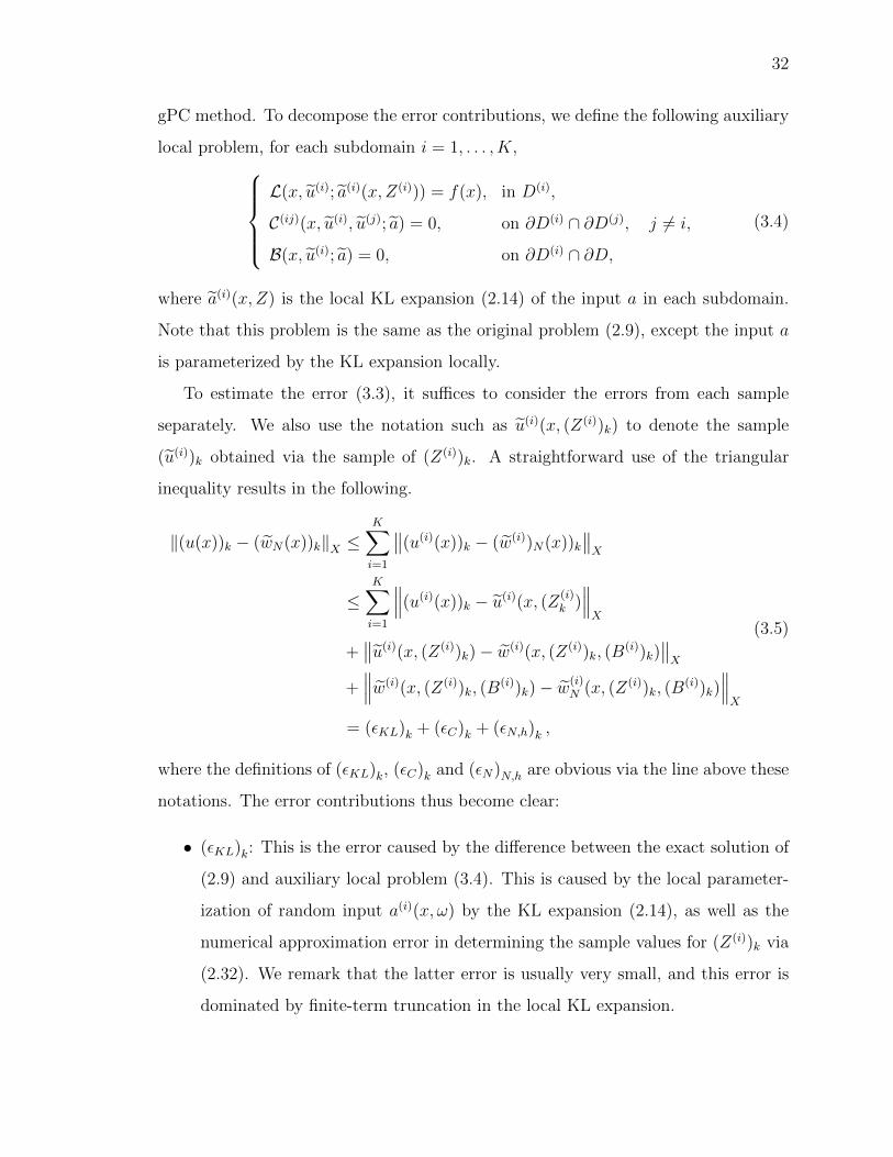
gPC method. To decompose the error contributions, we define the following auxiliary

local problem, for each subdomain i = 1, . . . , K,8>>><

>>>:

L(x, eu(i);ea(i)(x, Z(i))) = f(x), in D(i),

C(ij)(x, eu(i), eu(j);ea) = 0, on @D(i) \ @D(j), j 6= i,

B(x, eu(i);ea) = 0, on @D(i) \ @D,

(3.4)

where ea(i)(x, Z) is the local KL expansion (2.14) of the input a in each subdomain.

Note that this problem is the same as the original problem (2.9), except the input a

is parameterized by the KL expansion locally.

To estimate the error (3.3), it su�ces to consider the errors from each sample

separately. We also use the notation such as eu(i)(x, (Z(i))k) to denote the sample

(eu(i))k obtained via the sample of (Z(i))k. A straightforward use of the triangular

inequality results in the following.

k(u(x))k � ( ewN(x))kkX KX

i=1

��(u(i)(x))k � ( ew(i))N(x))k��X

KX

i=1

��(u(i)(x))k � eu(i)(x, (Z(i)k )��X

+��eu(i)(x, (Z(i))k)� ew(i)(x, (Z(i))k, (B

(i))k)��X

+�� ew(i)(x, (Z(i))k, (B

(i))k)� ew(i)N (x, (Z(i))k, (B

(i))k)��X

= (✏KL)k + (✏C)k + (✏N,h)k ,

(3.5)

where the definitions of (✏KL)k, (✏C)k and (✏N)N,h are obvious via the line above these

notations. The error contributions thus become clear:

• (✏KL)k: This is the error caused by the di↵erence between the exact solution of

(2.9) and auxiliary local problem (3.4). This is caused by the local parameter-

ization of random input a(i)(x,!) by the KL expansion (2.14), as well as the

numerical approximation error in determining the sample values for (Z(i))k via

(2.32). We remark that the latter error is usually very small, and this error is

dominated by finite-term truncation in the local KL expansion.

33

• (✏C)k: This error is caused by the di↵erence between the auxiliary local problem

(3.4) and the subdomain problem (2.19), with its contribution from determin-

ing the boundary parameter samples (B(i))k via the interface problem (2.33).

We remark that the numerical error in solving the system of equations (e.g.

Newton’s method, fast gradient descent method, etc.) in (2.33) is usually very

small and can be neglected.

• (✏N,h)k: The standard error for solving the local problem (2.19), which is equiv-

alent to (2.25) and (2.26) for linear problems, in each subdomain. This error

consists of the approximation error in both the random space and the physical

space. For random space, one can employ any standard stochastic method, such

as the Nth-order gPC method used in the Chapter of numerical examples; and

for physical space, any standard discretization such as finite elements or finite

di↵erence with the discretization parameter h can be used.

The above argument provides only a guideline of the error contributions. A de-

tailed error analysis shall be conducted for a given governing problem, which will

determine the proper norm k · kX to be used in the physical space. (Such kind of

detailed analysis will be discussed in the section of future work.) It is clear from the

discussion that the predominant error contributions stem from the local parameteri-

zation error (✏KL)k, primarily due to the truncation of the local KL expansion, and

the finite-order gPC approximation error (✏N,h)k, as long as the discretization error

in the physical space is su�ciently small.

3.2 Computational Complexity

To solve the original problem (2.1), the standard approach is to solve the param-

eterized problem (2.7), in the d-dimensional random space and the global domain D.

When the random input a(x,!) has short correlation length, e.g. a relatively rough

path in visualization, the random dimension can be very high, d � 1 and make the

problem prohibitively expensive to solve.

34

The local gPC method presented here seeks to solve (2.1) in a collection of non-

overlapping subdomains {D(i)}Ki=1. In each subdomain, the subdomain problem (2.12)

is defined via an artificial boundary condition. The random input a(x,!) is param-

eterized locally in by d(i)-dimensional random parameters. The artificial boundary

condition is parameterized by the standard basis functions in physical domain, which

results in d(i)� parameters. This makes the subdomain problem reside in ed(i) = d(i)+d(i)�

dimensional parameter space.

For linear governing equations, the subdomain problem can be readily solved

(d(i)� + 1) times in the d(i)-dimensional random space, as in (2.25) and (2.26). Since

d(i) is determined by the local parameterization of the random input a(x,!), it can

be significantly smaller than d, as demonstrated in Figure 2.1 and Figure 2.2. Since

d(i) ⌧ d, the local gPC induces significantly less simulation burden, even though the

subdomain problems need to be solved (d(i)� +1) times. Also, because the local random

dimension d(i) is much lower, typically of O(1), one can solve the local problem using

higher order methods to achieve high accuracy.

An added cost in the local gPC method, which is not explicitly present in the

traditional global gPC methods, is incurred when the samples of the correct global

solutions are constructed. This involves (i) using the samples of the input a to

determine the parameters Z(i) in each subdomains; and (ii) for each such sample

solving a system of equations from the coupling conditions to determine the boundary

parameters B(i). The simulation cost of the first step is negligible. The second

step requires one to solve a system of (linear) equations and does not require any

(stochastic) PDE solution.

3.3 Choice of Subdomain and Spatial Discretization.

The local gPC method represents a rather general approach and is not tied up

to a certain spatial discretization. One may choose any feasible spatial discretization

schemes for the governing equation (2.1), e.g., FEM, finite di↵erence/volume, etc.

35

The determination of the subdomains is solely based on the desired relative cor-

relation length of a. In practice, one should choose the subdomains with su�ciently

small size so that the relative correlation length of a is reasonably large. This ensures

the fast decay of KL eigenvalues (2.14) in each subdomain and the low dimension-

ality of the subdomain problem (2.19). It is also convenient to let the interfaces

between the subdomains to align with the physical meshes. By doing so, the spatial

basis functions can be directly used to approximate the artificial boundary conditions

(2.18).

Even though smaller subdomains are preferred to reduce the dimensionality of

the local gPC problem, we caution that the size of the subdomains can not be ex-

ceedingly small. Smaller subdomains results in a larger number of subdomains, and

consequently, a larger system of equations to solve for the interface problem (2.33).

Therefore, in practice, the choice of the size of the subdomains should be a balanced

decision.

37

4. FURTHER VALIDATION

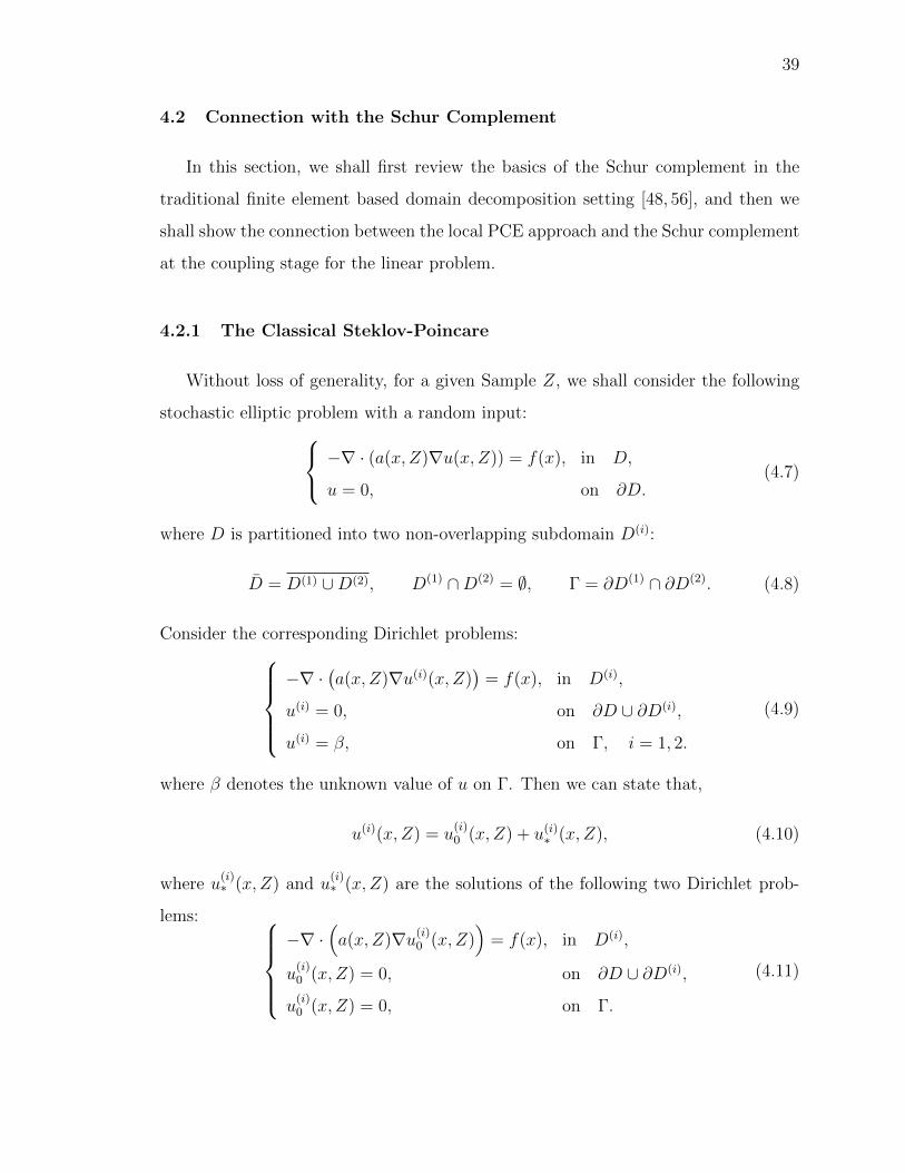
4.1 Application to Stochastic Elliptic Equation

In this section we use stochastic elliptic equation to illustrate the details of the

local gPC method. We consider

8<

:�r · (a(x,!)ru(x,!)) = f(x), x 2 D,

u = g(x) x 2 @D.(4.1)

Without loss of generality, we assume the right-hand side and the boundary conditions

are deterministic. The only random input is via the di↵usivity a(x,!). Our focus

is on the case when a has short correlation length, since it requires large number of

random parameters to parametrize the di↵usivity a(x,!), hence much more attention

must be paid to the computational cost.

4.1.1 Subdomain Problems and Interface Conditions

Let D(i), i = 1, . . . , K, be a set of non-overlapping subdomains, then the problem

(4.1) is equivalent to the following problem.

8>>>><

>>>>:

�r ·�a(x,!)ru(i)(x,!)

�= f (i)(x), in D(i),

u(i) = u(j), n · aru(i) = n · aru(j), on @D(i) \ @D(j),

u(i) = g(x), on @D,

(4.2)

where n is the unit normal vector at the interfaces. The coupling conditions for the

elliptic problem are defined by enforcing the continuity in both the solution and the

flux. That is, along the interfaces @D(i) \ @D(j), we have

u(i) = u(j), n ·ru(i) = n ·ru(j), (4.3)

38

Note that these are the widely used coupling conditions for elliptic equations in do-

main decomposition methods to ensure well posedness of the problem (see [54, 55]).

(4.3) shows the pointwise continuity of the solution itself and the flux term. It is also

valid to apply a slightly weaker condition on the flux, which we will discuss and make

a comparison in the following sections of Schur complement system.

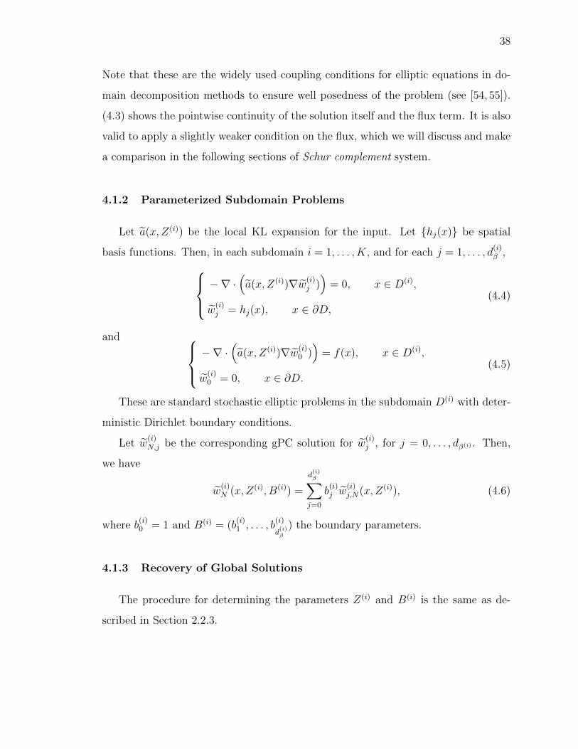
4.1.2 Parameterized Subdomain Problems

Let ea(x, Z(i)) be the local KL expansion for the input. Let {hj(x)} be spatial

basis functions. Then, in each subdomain i = 1, . . . , K, and for each j = 1, . . . , d(i)� ,

8><

>:

�r ·⇣ea(x, Z(i))r ew(i)

j )⌘= 0, x 2 D(i),

ew(i)j = hj(x), x 2 @D,

(4.4)

and 8><

>:

�r ·⇣ea(x, Z(i))r ew(i)

0 )⌘= f(x), x 2 D(i),

ew(i)0 = 0, x 2 @D.

(4.5)

These are standard stochastic elliptic problems in the subdomain D(i) with deter-

ministic Dirichlet boundary conditions.

Let ew(i)N,j be the corresponding gPC solution for ew(i)

j , for j = 0, . . . , d�(i) . Then,

we have

ew(i)N (x, Z(i), B(i)) =

d(i)�X

j=0

b(i)j ew(i)j,N(x, Z

(i)), (4.6)

where b(i)0 = 1 and B(i) = (b(i)1 , . . . , b(i)d(i)�

) the boundary parameters.

4.1.3 Recovery of Global Solutions

The procedure for determining the parameters Z(i) and B(i) is the same as de-

scribed in Section 2.2.3.

39

4.2 Connection with the Schur Complement

In this section, we shall first review the basics of the Schur complement in the

traditional finite element based domain decomposition setting [48, 56], and then we

shall show the connection between the local PCE approach and the Schur complement

at the coupling stage for the linear problem.

4.2.1 The Classical Steklov-Poincare

Without loss of generality, for a given Sample Z, we shall consider the following

stochastic elliptic problem with a random input:8<

:�r · (a(x, Z)ru(x, Z)) = f(x), in D,

u = 0, on @D.(4.7)

where D is partitioned into two non-overlapping subdomain D(i):

D = D(1) [D(2), D(1) \D(2) = ;, � = @D(1) \ @D(2). (4.8)

Consider the corresponding Dirichlet problems:8>>><

>>>:

�r ·�a(x, Z)ru(i)(x, Z)

�= f(x), in D(i),

u(i) = 0, on @D [ @D(i),

u(i) = �, on �, i = 1, 2.

(4.9)

where � denotes the unknown value of u on �. Then we can state that,

u(i)(x, Z) = u(i)0 (x, Z) + u(i)

⇤ (x, Z), (4.10)

where u(i)⇤ (x, Z) and u(i)

⇤ (x, Z) are the solutions of the following two Dirichlet prob-

lems: 8>>><

>>>:

�r ·⇣a(x, Z)ru(i)

0 (x, Z)⌘= f(x), in D(i),

u(i)0 (x, Z) = 0, on @D [ @D(i),

u(i)0 (x, Z) = 0, on �.

(4.11)

40

and 8>>><

>>>:

�r ·⇣a(x, Z)ru(i)

⇤ (x, Z)⌘= 0, in D(i),

u(i)⇤ (x, Z) = 0, on @D [ @D(i),

u(i)⇤ (x, Z) = �, on �.

(4.12)

For each i = 1, 2, we denote

Gif := u(i)0 (x, Z), Hi� := u(i)

⇤ (x, Z). (4.13)

By enforcing flux continuity at the interface � weakly:

Z

�

a(x, Z)@

@nu(1)(x, Z)vdx =

Z

�

a(x, Z)@

@nu(2)(x, Z)vdx, v 2 ⇤, (4.14)

where

⇤ := {⌘ 2 H1/2(�)|⌘ = v|� for a suitable v 2 H0(D)}. (4.15)

then � satisfiesZ

�

a(x, Z)(@

@nu(1)0 (x, Z) +

@

@nu(1)⇤ (x, Z))vdx

=

Z

�

a(x, Z)(@

@nu(2)0 (x, Z) +

@

@nu(2)⇤ (x, Z))vdx,

(4.16)

After rearrangement, we get

Z

�

a(x, Z)(@

@nu(1)⇤ (x, Z)� @

@n)u(2)

⇤ (x, Z) =

Z

�

a(x, Z)(@

@nu(2)0 (x, Z)� @

@nu(1)0 (x, Z))vdx,

(4.17)

this is so called the weak form of the Steklov-Poincare interface equation:

Z

�

S�vdx =

Z

�

�vdx, (4.18)

where

S� = a(x, Z)2X

i=1

@

@n(i)u(i)⇤ (x, Z) = a(x, Z)

2X

i=1

@

@n(i)Hi�,

� = �a(x, Z)2X

i=1

@

@n(i)u(i)0 (x, Z) = �a(x, Z)

2X

i=1

@

@n(i)Gif.

(4.19)

41

4.2.2 Steklov-Poincare in Local PCE

The local PCE starts with the parameterized subdomain problems:8>>><

>>>:

�r ·�a(i)(x, Z)rw(i)(x, Z)

�= f(x), in D(i),

w(i)(x, Z) = 0, on @D [ @D(i),

w(i)(x, Z) = �(i), on �,

(4.20)

where �(i) is parameterized as follows:

�(i) =

d(i)�X

i=1

b(i)j hj(x). (4.21)

Then the local solution in each subdomain can be represented as follows:

w(i)(x, Z) = w(i)0 + w(i)

⇤ , (4.22)

where

w(i)⇤ =

d(i)�X

i=1

b(i)j wj(x, Z), (4.23)

and w(i)j (x, Z) are the solutions of the following Dirichlet problems:

• for j = 0,8<

:�r ·

⇣a(i)(x, Z)rw(i)

0 (x, Z)⌘= f(x), in D(i),

w(i)0 (x, Z) = 0, on @D(i).

(4.24)

• for j = 1, . . . , d(i)� ,8<

:�r ·

⇣a(i)(x, Z)rw(i)

j (x, Z)⌘= 0, in D(i),

w(i)j (x, Z) = hj(x), on @D(i).

(4.25)

For each i = 1, 2, we denote

Gif := w(i)0 (x, Z), Hihj(x) := w(i)

j (x, Z). (4.26)

Then it is obvious thatnX

j=1

b(i)j Hihj(x) = Hi� := w(i)⇤ . (4.27)

42

By enforcing nodal and flux continuity at the interface � weakly:

�(1)(x, Z) = �(2)(x, Z) = �(x, Z),Z

�

a(1)(x, Z)@

@nw(1)(x, Z)vdx =

Z

�

a(2)(x, Z)@

@nw(2)(x, Z)vdx,

(4.28)

the � satisfiesZ

�

a(1)(x, Z)(@

@nw(1)

0 (x, Z)+@

@nw(1)

⇤ (x, Z))vdx

=

Z

�

a(2)(x, Z)(@

@nw(2)

0 (x, Z) +@

@nw(2)

⇤ (x, Z))vdx,

(4.29)

After rearrangement,Z

�

(a(1)(x, Z)@

@nw(1)

⇤ (x, Z)� a(2)(x, Z)@

@nw(2)

⇤ (x, Z))vdx

=

Z

�

(a(2)(x, Z)@

@nw(2)

0 (x, Z)� a(1)(x, Z)@

@nw(1)

0 (x, Z))vdx.(4.30)

We then get the weak form of the approximated Steklov-Poincare interface equation:Z

�

S�vdx =

Z

�

�vdx, (4.31)

where

S� =2X

i=1

a(i)(x, Z)@

@n(i)w(i)

⇤ (x, Z) =2X

i=1

a(i)(x, Z)@

@n(i)Hi�,

� = �2X

i=1

a(i)(x, Z)@

@n(i)w(i)

0 (x, Z) = �2X

i=1

a(i)(x, Z)@

@n(i)Gif.

(4.32)

Compared with (4.18), the di↵erence of both sides of the Steklov-Poincare interface

equation can be clearly seen as follows:

S� � S� = (S � S)� + S(� � �)

=2X

i=1

⇥a(x, Z)

@

@n(i)Hi � a(i)(x, Z)

@

@n(i)Hi

⇤� +

2X

i=1

a(i)(x, Z)@

@n(i)Hi(� � �),

�� = �2X

i=1

⇥a(x, Z)

@

@n(i)Gi � a(i)(x, Z)

@

@n(i)Gi

⇤f.

(4.33)

43

4.2.3 The Classical Schur Complement

Without loss of generality, we shall consider the following stochastic elliptic prob-

lem with a random input, parameterized via a global KL expansion:8<

:�r · (a(x, Z)ru(x, Z)) = f(x), in D,

u = 0, on @D.(4.34)

where D is partitioned into two non-overlapping subdomain D(i):

D = D(1) [D(2), D(1) \D(2) = ;, � = @D(1) \ @D(2). (4.35)

The corresponding variational problem reads: find u 2 H10 such that

Z

D

a(x, Z)ru ·rvdx =

Z

D

fvdx, v 2 H10 . (4.36)

Let K be the finite element mesh of D and Vh is the finite element space defined on K.

For a given sample Z, the classical finite element approximation seeks uh 2 Vh ⇢ H10

such that Z

D

a(x, Z)ruh ·rvhdx =

Z

D

fvhdx, vh 2 Vh, (4.37)

which gives rise to the following linear system:

Au = F, (4.38)

where

A =

2

6664

A(1)II 0 A(1)

I�

0 A(2)II A(2)

I�

A(1)�I A(2)

�I A��

3

7775, u =

2

6664

u(1)I

u(2)I

u�

3

7775, F =

2

6664

F (1)I

F (2)I

F�

3

7775. (4.39)

The unknown coe�cients vector u can be split into two parts: the contribution from

interior nodes of the subdomains u(i)I and the contribution from the interface nodes

u�. A(i)II represents the interaction between the interior nodes. A(i)

I� represents the

interaction between the interior nodes and interface nodes in i-th subdomain. A��

represents the interaction between the interface nodes.

44

By performing block Gauss elimination of A, we get

2

6664

A(1)II 0 A(1)

I�

0 A(2)II A(2)

I�

0 0 S

3

7775u =

2

6664

F (1)I

F (2)I

g�

3

7775. (4.40)

where S is the so-called Schur complement matrix,

S = A�� A(1)�IA

(1)�1

II A(1)I� � A(2)

�IA(2)�1

II A(2)I� , (4.41)

g� = F� � A(1)�IA

(1)�1

II F (1)I � A(2)

�IA(2)�1

II F (2)I , (4.42)

where

F (i) =

2

4F(i)I

F (i)�

3

5 , A(i) =

2

4A(i)II A(i)

I�

A(i)�I A(i)

��

3

5 , (4.43)

are the right hand sides and local sti↵ness matrices for the elliptic problems with a

Dirichlet boundary condition on @D \ � and a Neumann boundary condition on �,

we then have

A�� = A(1)�� + A(2)

��, F� = F (1)� + F (2)

� . (4.44)

With above notations, we find the Schur complement system for u� as follows:

Su� = g�. (4.45)

and the inner unknowns can be recovered by

u(i)I = A(i)�1

II (F (i)I � A(i)

I�u�) (4.46)

following the matrix equation (4.40)

4.2.4 The Local PCE Approach - Local Problem

We discovered a connection between Schur complement and our local polynomial

chaos expansion method.

45

The local PCE approach starts with subdomain problems with Dirichelet condition

on the interface:8<

:�r ·

�a(i)(x, Z(i))rw(i)(x, Z(i))

�= f (i), in D(i), i = 1, 2,

w(i) = �(i), on �,(4.47)

where �(i) is treated as an auxiliary variable. Similar with Section 4.2.3, for the same

global finite element mesh K, a finite element approximation seeks w(i)h 2 Vh(D(i))

such that

Z

D(i)

a(i)(x, Z(i))rw(i)h ·rvhdx =

Z

D(i)

fvhdx, vh 2 V 0h (D

(i)), (4.48)

with the boundary condition w(i)h|� = B(i), where V 0

h (D(i)) := {vh 2 Vh(D(i)) : vh|� =

0}. This leads to the following local linear system:

2

4A(i)II A(i)

I�

0 I

3

5

2

4w(i)I

w�

3

5 =

2

4F(i)I

B(i)

3

5 , i = 1, 2, (4.49)

where I is an identity matrix. It is easy to see that the interior components can be

found by

w(i)I = A(i)�1

II (F (i)I � A(i)

I�B(i)). (4.50)

It can be observed that the interior unknowns w(i)I can be represented in terms of

B(i) at the interface. Recall that given the linearity of the elliptic problem with

parameterized Dirichlet boundary condition, we only need to solve (d(i)� +1) problems

((2.25) and (2.26)) in d-dimensional spaces for local random variable Z(i) for each

subdomain, i.e., in each subdomain D(i), we solve the following linear systems,

(1) the homogeneous system with nonzero Dirichlet boundary condition,

2

4A(i)II A(i)

I�

0 I

3

5

2

4w(i)I,m

w(i)�,m

3

5 =

2

4 0

em

3

5 , m = 1, 2, . . . , d(i)� , (4.51)

where d(i)� = number of degrees of freedom in local boundary �, and em is the

m-th column vector of identity matrix Id(i)� ⇥d

(i)�.

46

(2) the nonhomogeneous system with zero Dirichlet boundary condition,2

4A(i)II A(i)

I�

0 I

3

5

2

4w(i)I,0

w(i)�,0

3

5 =

2

4F(i)I

0

3

5 . (4.52)

By (4.51) and (4.52), we get

A(i)II w

(i)I,m + A(i)

I�em = 0, m = 1, 2, . . . , d(i)� , (4.53)

A(i)II w

(i)I,0 = F (i)

I , (4.54)

hence,

w(i)I,m = �A(i)�1

II A(i)I�em, m = 1, 2, . . . , d(i)� , (4.55)

w(i)I,0 = A(i)�1

II F (i)I . (4.56)

We store these local solutions w(i)I,m and pass them into the assembly of the inter-

face linear system. Assemble all w(i)I,m together with em as follows. We denote the

prolongation (linear) operator E(i),

E(i) =

2

64w(i)

I,1 w(i)I,2, . . . , w(i)

I,d(i)�

e1 e2, . . . , ed(i)�

3

75 , (4.57)

We denote the upper portion of E(i) as E(i)I . By the derivation in (4.57), we get,

E(i)I =

w(i)

I,1 w(i)I,2, . . . , w(i)

I,d(i)�

�= �A(i)�1

II A(i)I�, (4.58)

And the lower portion of E(i) is simply an identity matrix I. Therefore, we re-write

the linear operator E(i) as,

E(i) =

2

4�A(i)�1

II A(i)I�

I

3

5 , (4.59)

We also denote the following vector as e(i)0 for the nonhomogeneous solution,

e(i)0 =

2

4w(i)I,0

0

3

5 =

2

4A(i)�1

II F (i)I

0

3

5 , (4.60)

47

Operator E(i) and vector e(i)0 provide the map from the local boundary degrees of

freedom to the whole subdomain’s degrees of freedom. Recall the representation of

local solution w(i)(x,B(i)) (2.27) of the subdomain problem, we then have

w(i) =

2

4w(i)I

w(i)�

3

5 = E(i)B(i) + e(i)0 . (4.61)

This map helps to construct a full local FE solution w(i) from the unknown local

boundary degrees of freedom B(i). To recover B(i), we need to couple the local

solutions at each subdomain together.

4.2.5 The Local PCE Approach - The Interface Problem

To couple the solutions at di↵erent subdomains, we enforce C0 continuity strongly

and enforce the local flux continuity weakly at the interface � by seeking wh =P2

i=1 w(i)h ID(i) 2 Vh such that

w(1)h = w(2)

h , on �Z

�

a(1)(x, Z(1))@w(1)

h

@n1vhds =

Z

�

a(2)(x, Z(2))@w(2)

h

@n2vhds, vh 2 Th,

(4.62)

where Th is the space spanned by all nodal bases on �, i.e., Th := Vh(�) and n1 = �n2.

By the Green’s first identity,

Z

�

a(i)(x, Z(i))@w(i)

h

@nivhds =

Z

D(i)

⇥r ·�a(i)(x, Z(i))rw(i)(x, Z(i))

�vh⇤dx

+

Z

D(i)

ha(i)(x, Z(i))rw(i)

h ·rvhidx

=

Z

D(i)

h�fvh + a(i)(x, Z(i))rw(i)

h ·rvhidx.

(4.63)

Substitute (4.63) into (4.62), the interface problem becomes that we seeks wh =P2

i=1 w(i)h ID(i) 2 Vh such that

2X

i=1

Z

D(i)

a(i)(x, Z(i))rw(i)h ·rvhdx =

2X

i=1

Z

D(i)

fvhdx, vh 2 Th. (4.64)

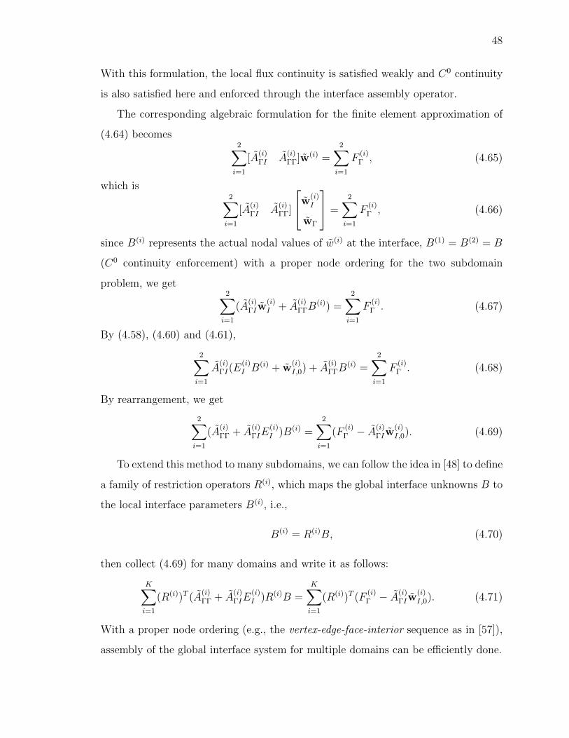
48

With this formulation, the local flux continuity is satisfied weakly and C0 continuity

is also satisfied here and enforced through the interface assembly operator.

The corresponding algebraic formulation for the finite element approximation of

(4.64) becomes2X

i=1

[A(i)�I A(i)

��]w(i) =

2X

i=1

F (i)� , (4.65)

which is2X

i=1

[A(i)�I A(i)

��]

2

4w(i)I

w�

3

5 =2X

i=1

F (i)� , (4.66)

since B(i) represents the actual nodal values of w(i) at the interface, B(1) = B(2) = B

(C0 continuity enforcement) with a proper node ordering for the two subdomain

problem, we get2X

i=1

(A(i)�Iw

(i)I + A(i)

��B(i)) =

2X

i=1

F (i)� . (4.67)

By (4.58), (4.60) and (4.61),

2X

i=1

A(i)�I(E

(i)I B(i) + w(i)

I,0) + A(i)��B

(i) =2X

i=1

F (i)� . (4.68)

By rearrangement, we get

2X

i=1

(A(i)�� + A(i)

�IE(i)I )B(i) =

2X

i=1

(F (i)� � A(i)

�Iw(i)I,0). (4.69)

To extend this method to many subdomains, we can follow the idea in [48] to define

a family of restriction operators R(i), which maps the global interface unknowns B to

the local interface parameters B(i), i.e.,

B(i) = R(i)B, (4.70)

then collect (4.69) for many domains and write it as follows:

KX

i=1

(R(i))T (A(i)�� + A(i)

�IE(i)I )R(i)B =

KX

i=1

(R(i))T (F (i)� � A(i)

�Iw(i)I,0). (4.71)

With a proper node ordering (e.g., the vertex-edge-face-interior sequence as in [57]),

assembly of the global interface system for multiple domains can be e�ciently done.

49

It is almost clear that (4.71) shows a same formulation of our interface problem

compared to the Schur complement system for interface nodes u� in (4.45). To verify

that, firstly, disregard the term (R(i))T and R(i) on both sides (since they are just

locators to help ensure the correct place to keep a corresponding matrix for each

interface edges); secondly, perform a substitution given by (4.58) and (4.56), one get,

KX

i=1

(A(i)�� A(i)

�IA(i)�1

II A(i)I�)B

(i) =KX

i=1

(F (i)� � A(i)

�IA(i)�1

II F (i)I ). (4.72)

With the proper locator operator, one can conclude that this derivation is building

on the same numerical base as Schur complement system, which we denote as the

following concise form,

SB = g, (4.73)

In practice, we need to solve the encapsulation problem to build the gPC surrogate

(wI,m)(i)N to replace w(i)

I,m,m = 1, . . . , d(i)� and therefore (E(i)I )N is the counterpart of

E(i)I .

Then the interface problem is replaced by the approximated interface problem:

SNBN = gN , (4.74)

where

SN =2X

i=1

⇥A(i)

�� A(i)�I(E

(i)I )N

⇤, (4.75)

gN =2X

i=1

⇥F (i)� � A(i)

�I(w(i)I,0)N

⇤. (4.76)

and the correpsonding interior unknowns (w(i)I )N can be approximated by

(wI)(i)N = A(i)�1

II (F (i)I � A(i)

I�BN). (4.77)

Note that we get back to the two subdomains illustration settings, since it is simple

and straightforward to show the idea with the consideration of simple notations.

Next, we shall examine the di↵erence between the Schur complement system (4.46)

and the approximated version (4.74) for each sample in the following steps:

50

(1) We first examine the the di↵erence between the Schur complement matrix and

the approximated one:

SN =2X

i=1

(A(i)�� A(i)

�IA(i)�1

II A(i)I�)

+2X

i=1

⇥(A(i)

�� A(i)��)� (A(i)

�IA(i)�1

II A(i)I� � A(i)

�IA(i)�1

II A(i)I�)⇤

�2X

i=1

A(i)�I

⇥(E(i)

I )N � E(i)I

⇤

= S + �S,

(4.78)

where

�S =2X

i=1

⇥(A(i)

��A(i)��)�(A

(i)�IA

(i)�1

II A(i)I��A

(i)�IA

(i)�1

II A(i)I�)⇤�

2X

i=1

A(i)�I

⇥(E(i)

I )N�E(i)I

⇤.

(4.79)

Observe that the first summation is the error due to local KL expansion and the

second summation is the error due to the surrogate by the sparse grid. We then

assume ||�S|| = ✏S = C1(✏KL + ✏N,h), where ✏KL and ✏N,h denote the error due

to the local KL expansion and the error due to the surrogate of the subdomain

problems respectively.

(2) We next examine the the di↵erence for the right-hand sides:

gN =2X

i=1

(F�(i) � A(i)�IA

(i)�1

II F (i)I )

�2X

i=1

(A(i)�IA

(i)�1

II F (i)I � A(i)

�IA(i)�1

II F (i)I )

�2X

i=1

A(i)�I

⇥(w(i)

I,0)N �w(i)I,0

⇤

= g + �g,

(4.80)

where

�g = �2X

i=1

(A(i)�IA

(i)�1

II F (i)I � A(i)

�IA(i)�1

II F (i)I )�

2X

i=1

A(i)�I

⇥(w(i)

I,0)N �w(i)I,0

⇤. (4.81)

51

Similarly, we observe that the first summation is the error due to local KL

expansion and the second summation is the error due to the surrogate by the

sparse grid. We assume ||�g|| = ✏g = C2(✏KL + ✏N,h).

(3) Finally, we examine the di↵erence between BN and u� through a appropriate

vector norm and consistent matrix norm, let BN = u� + �u� and substitute

them into (4.74), we have

(S + �S)(u� + �u�) = g + �g. (4.82)

which leads to

�u� = (S + �S)�1(�g � �Su�)

= (I + S�1�S)�1S�1(�g � �Su�).(4.83)

Assume we can limit the local KL expansion error and the surrogate error by

sparse grid under a certain level, i.e., ✏KL ⌧ 1 and ✏N,h ⌧ 1, then we can get

||�S|| ✏S ⌧ 1 and ||�g|| ✏g ⌧ 1. As a result, we have the following estimate

for the interface parameters(unknowns) u�:

||�u�|| = ||(I + S�1�S)�1S�1(�g � �Su�)||

||S�1|||1� ||S�1||||�S|||(||�S||||u�||+ ||�g||)

||S�1||||S|||1� ||S�1||||S|| ||�S||||S|| |

(||�S||||S|| +

||�g||||S||||u�||

)||u�||

=(S)

|1� (S) ||�S||||S|| |(||�S||||S|| +

||�g||||S||||u�||

)||u�||

(S)

|1� (S) ||�S||||S|| |(||�S||||S|| +

||�g||||g|| )||u�||

(S)

|1� (S) ✏S||S|| |

(✏S||S|| +

✏g||g||)||u�||

(4.84)

52

where (S) is condition number of Schur complement matrix. And by (4.46)

and (4.77), we have following error estimate for the interior unknowns,

||u(i)I � (wI)

(i)N || = ||A(i)�1

II (F (i)I � A(i)

I�u�)� A(i)�1

II (F (i)I � A(i)

I�BN)||

= ||A(i)�1

II (F (i)I � A(i)

I�u�)� A(i)�1

II (F (i)I � A(i)

I�(u� + �u�))||

= ||(A(i)�1

II � A(i)�1

II )F (i)I + (A(i)�1

II A(i)I� � A(i)�1

II A(i)I�)u� + A(i)�1

II A(i)I��u�||

||(A(i)�1

II � A(i)�1

II )F (i)I ||+ ||(A(i)�1

II A(i)I� � A(i)�1

II A(i)I�)||||u�||

+ ||A(i)�1

II A(i)I�||||�u�||

C3✏KL||F (i)I ||+ C4✏KL||u�||+ C5||�u�||

(4.85)

This completes the exposition of the connection between the Schur complement

and the local PCE method. It is clear that the di↵erence between two approaches

are mainly due to local KL expansion and the polynomial chaos approximation of the

solutions of the subdomain problems. We have made a bound of such errors.

4.3 A Practical Algorithm

Based on the analysis above, we now present a practical algorithm of the local

PCE method for the linear problems involving six steps and we shall highlight e�cient

implementation strategies for some important steps as follows:

(1) Compute the local KL expansion (2.14) on each subdomain by solving the local

eigenvalue problems (2.15) and the local projection (2.16).

(2) Solve the i-th subdomain problems (2.25) and (2.26) with local parameterized

random inputs and Dirichelet boundary conditions to get the local solution

w(i)N,j, i = 1, . . . , K, j = 0, . . . , d(i)� .

(3) Store A(i)�I , A

(i)�� (essentially the whole row corresponding to the interface �).

(4) Form the interface problem matrix (Schur complement matrix).

53

(5) Solve the reduced system (4.74) to get the unknown coe�cients B(i)N .

(6) Recover the global solution via the local solutions:

wN(x, Z) =KX

i=1

d(i)�X

j=0

b(i)j w(i)N,j(x, Z

(i))ID(i) . (4.86)

1. The local projection (2.16) in step 1 can be rewritten as follows:

Z(i)j (!) =

1q�(i)j

Z

D(i)

(a(i)(x,!)� µ(i)a (x)) (i)

j (x)dx (4.87)

=d(i)X

k=1

p�kq�(i)j

Z

D(i)

k(x) (i)j (x)dx. (4.88)

Since in the finite element setting,

k =N(i)X

m=1

k,mh(i)m (x), (4.89)

(i)j =

N(i)X

m=1

(i)j,mh

(i)m (x), x 2 D(i), (4.90)

where h(i)m (x) is the finite element basis defined on the finite element mesh of i-

th subdomain D(i). N (i) is the number of the corresponding degrees-of-freedom

on the finite element mesh. k,m and (i)j,m are the eigenvector evaluated at the

mesh grid points. Define k = [ k,1 . . . k,N(i) ] and (i)

j = [ (i)j,1 . . .

(i)

j,N(i) ], (4.87)

can be approximated as follows:

Z(i)j (!) =

d(i)X

k=1

p�kq�(i)j

T

kM(i)

(i)

j Zk =d(i)X

k=1

P (i)jk Zk, (4.91)

where M (i) is the mass matrix computed on the finite element mesh of i-th sub-

domain D(i). It can be seen that once we know the eigenvalues and eigenvectors

of global and local KL expansions, P (i)jk can be precomputed, then local random

variables Z(i) can be easily computed.

2. For step 2, in order to evaluate w(i)N,j(x, z) e�ciently, we shall build a surrogate

for each subdomain by sparse grid interpolation.

54

3. For step 3, it seems that we have to assemble A(i) for a given new Z. However,

since the local KL expansion is a�ne,

A(i) = A(i)0 +

d(i)X

k=1

A(i)k Z(i)

k , (4.92)

where A(i)k that can be precomputed, corresponds to the sti↵ness matrix due to

the terms in the expansion of local KL expansion in (2.14). Therefore, given a

new sample Z, we only need to evaluate (4.92) and don’t need to go through

the assembly step in the local finite element solver again.

4. Since E(i)I (4.57) can be evaluated e�ciently by its gPC surrogate (E(i)

I )N with-

out evoking the local PDE solver and A(i) can be evaluated online e�ciently by

(4.92), step 4 can be done e�ciently by the following form:

KX

i=1

(R(i))T (A(i)�I + A(i)

��(E(i)I )N)R

(i)B =KX

i=1

(R(i))T (F (i)� � A(i)

�I(w(i)I,0)N). (4.93)

55

5. NUMERICAL EXAMPLES

In this section, we present numerical results to illustrate the e↵ectiveness of the

local gPC method. In the following exampless, we compare three di↵erent numerical

solutions. This is a typical way to separate the error contributions clearly and is

the similar approach discussed in 3.1. Here is a brief explanation of each numerical

solution:

• Local gPC solution.

This refers to the solution using the scheme what we discussed in the Section 2,

which involves employing domain decomposition with local KL expansion ap-

proximation for the global input a(x, Z), building the local subdomain solutions

by the sparse grid surrogate, and enforcing interface conditions by solving the

coupled interface system.

• Auxiliary reference solutions.

Given each realization of the KL expansion approximation of the global input

a(x, Z) as the deterministic input, we shall apply the same domain decomposi-

tion to get the realization of the local KL expansion a(x, Z(i)) and then use it as

the input to compute FEM solution on the mesh with the same total resolution

as the local gPC solution.

• Reference FEM solutions.

We solve the equation with the realizations of original global random field input

a(x, Z) on a full FEM mesh with the same total resolution as the local gPC

solution and auxiliary solution.

56

To examine the accuracy, we shall compare the di↵erences of the above solutions

in terms of following norm:

||(f(x))||l2,1 = max1kM

||(f(x))k||l2 (5.1)

where we denote (f(x)) = (f(x)1, . . . , f(x)M) to be a collection of function samples

and (f(x))k is the kth sample of the function f(x). In the following section, we shall

use M = 100 samples to compute the errors.

5.1 1D Elliptic Problem with Moderately Short Correlation Length

Consider the stochastic elliptic problem (4.1) in a one-dimensional physical domain

D = [0, 1]. The random di↵usivity field a(x,!) is set to be a process with a mean

value of 0.1 and a Gaussian covariance function,

C(x, y) = � exp

✓�(x� y)2

`2

◆, x, y 2 [0, 1], (5.2)

where ` is the correlation length and � controls the variance. In the following we will

set ` = 1/12 and � = 0.021. For this example we use quadratic finite-elements to

solve (4.1). We ensure that for any number K of the subdomains the total number of

elements on the global mesh (the union of all subspace meshes) is 400. For example, if

the global domain is decomposed into 10 subdomains, each subdomain will be solved

using 40 quadratic elements.

After decomposing the global domain into subdomains we construct local KLE

that approximate the global di↵usivity field on each subdomain. The local PCE

approach proposed in this paper leverages the fact that when the eigenvalues of the

local KLE decay rapidly, the stochastic dimension on a subdomain will be significantly

less than the global stochastic dimension. We have shown the result in 2.2.1, so we

skip the resulting plots in this chapter.

Given a KLE approximation on each subdomain the task of building a local poly-

nomial chaos expansion for the PDE on the global domain, requires building an

approximation of the PDE solution on each subdomain over the lower-dimensional

57

random variables of the subdomain. To compute the local gPC solution, we use

isotropic sparse grids [58, 59] to build a polynomial chaos expansion on each subdo-

main. Specifically, we use a sparse grid based upon the univariate Clenshaw-Curtis

quadrature rule and convert it to a Legendre PCE using a fast linear transformation

method developed in [60]. We emphasize again that in practice one may use any

convenient method to build the local gPC expansion in each subdomain.

Figure 5.1 plots the error in the local gPC solution against the number of sparse

grids subdomain solution samples at increasing gPC orders, using di↵erent dimensions

d of the local KL expansion. It is clear that the number of dimensions retained in

the local KL expansion significantly e↵ects the ability to generate accurate local gPC

solutions. With only one term retained (d = 1), the error induced by the local KL

expansion dominates and increasing the gPC order does not reduce the errors at all.

When more terms in the local KL expansion is used, i.e., d = 2, 3, 4, 5, we observe the

error convergence as higher order local gPC expansion is used and the errors saturate

the lower levels. The clearly demonstrate the error contribution from both the local

KL expansion (✏KL) and local gPC expansion (✏N,h), as discussed in (3.5).

The e�cacy of using local PCE to solve stochastic linear PDEs is demonstrated

emphatically in Figure 5.2. To generate this plot we built local PCE on each sub-

domain with a local KLE that was truncated at a dimension d that retained all

eigenvalues of the local KLE above machine precision. As the number of subdomains

K increases, the required dimensionality d of the local PCE decreases drastically and

results in much smaller errors and faster error convergence rate. We recall that at

lower dimensions d, building the local gPC expansion becomes much more e�cient.

We again remark that the local PCE method proposed here ensures that the PDE

on the global domain can be solved independently on each subdomain. Knowledge

of the solution on the other subdomains is only required when reconstructing the

solution on the global domain which is a post-processing step.

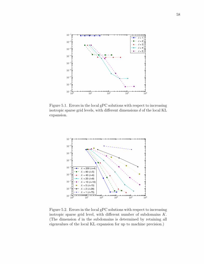
58

Figure 5.1. Errors in the local gPC solutions with respect to increasingisotropic sparse grid levels, with di↵erent dimensions d of the local KLexpansion.

Figure 5.2. Errors in the local gPC solutions with respect to increasingisotropic sparse grid level, with di↵erent number of subdomains K.(The dimension d in the subdomains is determined by retaining alleigenvalues of the local KL expansion for up to machine precision.)

59

5.2 2D Elliptic Problem with Moderate Correlation Length

We now present results for two-dimensional stochastic elliptic problem (4.1), with

the physical domain D = [�1, 1]2, with the right-hand-side of (4.1) set to f = 2+xy,

and a Dirichlet boundary condition of 2+x3y. The random di↵usivity field a(x,!) is

set to be the same process discussed in the local KL expansion in Figure 2.1, which

has a mean value of one and a Gaussian covariance function,

C(x, y) = exp

✓�kx� yk2

`2

◆, x, y 2 [�1, 1]2, (5.3)

where ` is the correlation length. Here we choose a moderate correlation length,

` = 1, and for clarity, we plot the first ten eigenvalues of the local KL expansion in

Figure. 5.3.

1 2 3 4 5 6 7 8 9 1010

−8

10−7

10−6

10−5

10−4

10−3

10−2

10−1

100

101

102

16 × 16 subdomains

8 × 8 subdomains

4 × 4 subdomains

Figure 5.3. The first ten eigenvalues of the local Karhunen-Loeveexpansion for covariance function C(x, y) = exp(�(x � y)2/`2) in[�1, 1]2 with ` = 1.

To compute the gPC expansion,we employ the high level sparse grids stochastic

collocation and then approximate the gPC orthogonal expansion coe�cients using

60

the sparse grids quadrature rule, see, for example, [10] for details. The reference

FEM solutions are computed over a 64⇥64 linear elements, which result in negligible

spatial discretization errors for this case. For subdomain decomposition, we utilize

three sets of subdomains: 4 ⇥ 4, 8⇥ 8, and 16⇥ 16. (The number of FEM elements

in each subdomain is adjusted in each case to keep the overall number of elements at

64⇥ 64.)

We first compute the errors in the local gPC solution against the auxiliary ref-

erence solutions. (Recall the local KL expansion errors are eliminated in this com-

parison.) In this case, we fix the local KL expansion at d(i) = 4 and vary the gPC

orders. The errors are shown in Figure 5.4, where we observe the fast and spectral

convergence with increasing order of gPC expansions.

1 2 3 410

−9

10−8

10−7

10−6

10−5

10−4

16 × 16 subdomains

8 × 8 subdomains

4 × 4 subdomains

Figure 5.4. Errors, measured against the auxiliary reference solutions,in the local gPC solutions with respect to increasing local gPC order.The local KL expansion is fixed at d(i) = 4.

61

Next we fix the local gPC order at N = 4, which results in very small errors

of O(10�9), as shown in Figure 5.4. We then compute the local gPC solutions

against the reference FEM solutions. Since the errors from the local gPC expansions

are small, we expect to see the dominance of the errors induced by the local KL

expansions. This is clearly illustrated in Figure 5.5, which plots the errors in the

local gPC solution with respect to the local KL truncation from d(i) = 1 to d(i) = 6.

The errors are much bigger than those in Figure 5.4, confirming that in this case the

biggest error contribution stems from the truncation error of the local KL expansion.

We observe that the error decay pattern is very similar to the local KL eigenvalue

decay, suggesting that the dominant errors are from the local KL expansion.

1 2 3 4 5 610

−5

10−4

10−3

10−2

10−1

16 × 16 subdomains

8 × 8 subdomains

4 × 4 subdomains

Figure 5.5. Errors in the local 4th-order gPC solutions with respectto increasing dimensionality of the local KL expansions, using 4⇥ 4,8⇥ 8, and 16⇥ 16 subdomains. (` = 1)

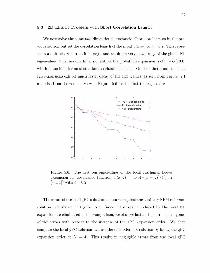
62

5.3 2D Elliptic Problem with Short Correlation Length

We now solve the same two-dimensional stochastic elliptic problem as in the pre-

vious section but set the correlation length of the input a(x,!) to ` = 0.2. This repre-

sents a quite short correlation length and results in very slow decay of the global KL

eigenvalues. The random dimensionality of the global KL expansion is of d ⇠ O(100),

which is too high for most standard stochastic methods. On the other hand, the local

KL expansions exhibit much faster decay of the eigenvalues, as seen from Figure 2.1

and also from the zoomed view in Figure 5.6 for the first ten eigenvalues.

1 2 3 4 5 6 7 8 9 1010

−4

10−3

10−2

10−1

100

101

102

16 × 16 subdomains

8 × 8 subdomains

4 × 4 subdomains

Figure 5.6. The first ten eigenvalues of the local Karhunen-Loeveexpansion for covariance function C(x, y) = exp(�(x � y)2/`2) in[�1, 1]2 with ` = 0.2.

The errors of the local gPC solution, measured against the auxiliary FEM reference

solution, are shown in Figure 5.7. Since the errors introduced by the local KL

expansion are eliminated in this comparison, we observe fast and spectral convergence

of the errors with respect to the increase of the gPC expansion order. We then

compare the local gPC solution against the true reference solution by fixing the gPC

expansion order at N = 4. This results in negligible errors from the local gPC

63

expansions. The errors are plotted in Figure 5.8, with respect to the increasing

dimensionality of the local KL expansions. We again notice the errors decay as more

terms in the local KL expansions are retained. We also note that the errors are

noticeably much larger than those in Figure 5.7, confirming that the predominant

contribution in the overall errors is from the truncation of the local KL expansion.

1 2 3 410

−9

10−8

10−7

10−6

10−5

10−4

16 × 16 subdomains

8 × 8 subdomains

4 × 4 subdomains

Figure 5.7. Errors, measured against the auxiliary reference solutions,in the local gPC solutions with respect to increasing local gPC order.The local KL expansion is fixed at d(i) = 4.

Finally, we emphasize that the errors introduced by truncation of the local KL

expansions will typically dominate the errors induced by other sources. The stochas-

tic elliptic problem is known to be very smooth in random space. In fact, for the

elliptic problems consider in this section, the stochastic solution is analytic in the

random space ( [4]). It is well known that for such analytic functions, gPC type

methods will converge very fast. In addition, since the subdomain problems of the

local gPC method of dimension O(1), we are able to compute reasonably high order

gPC expansions. The fast convergence and low dimensionality means that we can

64

1 2 3 4 5 610

−4

10−3

10−2

10−1

16 × 16 subdomains

8 × 8 subdomains

4 × 4 subdomains

Figure 5.8. Errors in the local 4th-order gPC solutions with respectto increasing dimensionality of the local KL expansions, using 4⇥ 4,8⇥ 8 and 16⇥ 16 subdomains. (` = 0.2)

65

easily drive the gPC error below the error introduced by the truncation of the local

KL expansions. Consequently, the error arising from the local KL expansions provide

the leading contribution to the total error of the local gPC method.

Errors induced by the input parameterization, e.g., either the standard global

KL expansion or the local KL expansion, should be considered a modeling error, as

they are not directly related to the algorithm itself. In fact, the local gPC method

presented in this paper can be more accurate in this sense, as it allows one the capture

more percentage of the KL eigenvalues because of the much faster eigenvalue decay

in the subdomains.

5.4 2D Di↵usion Equation with a Random Input in Layers

Consider the following two-dimensional stochastic elliptic problem8<

:�r · (a(x,!)ru(x,!)) = f(x), in D

u = g(x), on @D,(5.4)

with the physical domain D = [�1, 1]2, with the right-hand side f = 1, and zero

Dirichlet boundary condition. The random di↵usivity field a(x,!) has the covariance

function,

C(x, y) = exp

✓�kx� yk2

`2

◆, x, y 2 [�1, 1]2, (5.5)

where ` is the correlation length. Here we choose a short correlation length, ` = 0.2,

where the global KL expansion results in d = 200 random dimensions. We divide the

physical domain D = [�1, 1]2 into four rectangular layers with distinct mean values,

µa =

8>>>>>>><

>>>>>>>:

200, D1 = [�1, 1]⇥ [1/2, 1],

40, D2 = [�1, 1]⇥ [0, 1/2],

8, D3 = [�1, 1]⇥ [�1/2, 0],

4, D4 = [�1, 1]⇥ [�1,�1/2].

(5.6)

To compute the gPC surrogate, we employ the high level (with level 7) sparse grids

stochastic collocation and then approximate the gPC expansion coe�cients using the

66

Figure 5.9. A realization of the input random field a(x, Z) with dis-tinct means values in each layer indicated above and the correspondingfull finite element solution.

67

sparse grids quadrature rule (with level 7). The reference FEM solutions are computed

over a 64⇥ 64 linear elements, which result in negligible spatial discretization errors

for this case. For domain partitioning, we utilize three sets of subdomains: 4 ⇥ 4,

8 ⇥ 8, and 16 ⇥ 16 (the number of FEM elements in each subdomain is adjusted in

each case to keep the overall number of elements at 64⇥ 64).

Figure 5.9 shows one realization of the input random field a(x, Z) with distinct

means values in each layer indicated above. The corresponding full finite element

solution (reference solution) of the di↵usion problem in the domain D = [�1, 1]2 is

shown in Figure 5.10.

Figure 5.10. The corresponding full finite element solution (referencesolution) of the realization of the input a(x, Z) with distinct meansvalues in each layer indicated above.

We first compute the errors in the local gPC solution against the auxiliary refer-

ence solutions (recall the local KL expansion errors are eliminated in this comparison).

In this case, we fix the local KL expansion at d(i) = 4 and vary the gPC orders. The

errors are shown in Figure 5.11, where we observe the fast and spectral convergence

with increasing order of gPC expansions.

68

In the figures, for example, 16⇥16 subdomains means we have evenly partitioned

16 ⇥ 16 subdomains in D = [�1, 1]2, which gives 4 ⇥ 16 subdomains in each layer

region, and 4 ⇥ 4 linear elements in each subdomain to make the total resolution as

64⇥ 64 linear elements.

1 2 3 410

−7

10−6

10−5

10−4

16 × 16 subdomains

8 × 8 subdomains

4 × 4 subdomains

Figure 5.11. Errors, measured against the auxiliary reference solu-tions, in the local gPC solutions with respect to increasing gPC order.The local KL expansion is fixed at d(i) = 4.

Next we fix the local gPC order at N = 4, which results in very small errors of

O(10�7), as shown in Figure 5.11. We then compute the local gPC solutions against

the reference FEM solutions. Since the errors from the local gPC expansions are small,

we expect to see the dominance of the errors induced by the local KL expansions.

This is clearly illustrated in Figure 5.12, which plots the errors in the local gPC

solution with respect to the local KL truncation from d = 1 to d = 6. The errors are

much bigger than those in Figure 5.11 confirming that in this case the biggest error

contribution stems from the truncation error of the local KL expansion.

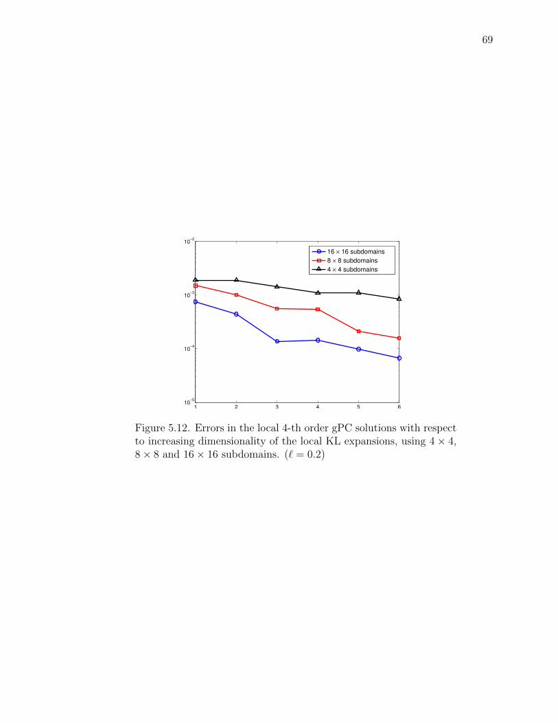
69

1 2 3 4 5 610

−5

10−4

10−3

10−2

16 × 16 subdomains

8 × 8 subdomains

4 × 4 subdomains

Figure 5.12. Errors in the local 4-th order gPC solutions with respectto increasing dimensionality of the local KL expansions, using 4⇥ 4,8⇥ 8 and 16⇥ 16 subdomains. (` = 0.2)

70

5.5 2D Di↵usion Equation with a Random Input in Di↵erent Direction

We now consider the two-dimensional stochastic elliptic problem8<

:�r · (a(x,!)ru(x,!)) = f(x), in D,

u = g(x), on @D,(5.7)

with the T-shaped physical domain D = Dh [Dv where Dh = [�3, 3] ⇥ [1, 3], Dv =

[�1, 1]⇥ [�3, 1), with the right-hand-side f = 1, and zero Dirichlet boundary condi-

tion on @D. In Dh the random di↵usivity field a(x,!) has x-directional covariance

functions,

C(x1, x01) = exp

✓�(x1 � x0

1)2

`2

◆, x1, x

01 2 [�3, 3], (5.8)

In Dv the random di↵usivity field a(x,!) has y-directional covariance functions,

C(x2, x02) = exp

✓�(x2 � x0

2)2

`2

◆, x2, x

02 2 [�3, 1], (5.9)

where ` is the correlation length. Here we choose a regular correlation length, ` = 0.4,

where the global KL expansion results in d = 40 random dimensions. We also set

the average value of both random field as µa = 10 hereafter. Figure 5.14 shows

one realization of the input random field a(x, Z) with distinct directional covariance

functions in Dh, and Dv and the corresponding full finite element solution (reference

solution) of the di↵usion problem in the T-shaped domain D.

We consider the T-shaped region D as the union of five square regions and apply

the same discretization procedure we employed before to set up rectangular subdo-

mains in each square region. Figure 5.15 shows a rough look of global mesh and the

skeleton degree of freedoms at the interface when the number of subdomains in each

square region is set as 4⇥ 4 and the number of FEM elements in each domain is set

as 4 ⇥ 4. In fact, all the crossed points indicate the actual unknowns in the inter-

face problem, while the solid points are boundary nodes fixed by Dirichlet boundary

conditions.

We again employ the high level sparse grids stochastic collocation (with level 7)

and then approximate the gPC expansion coe�cients using the sparse grids quadra-

ture rule (with level 7). The reference FEM solutions are computed over a 16⇥16⇥5

71

Figure 5.13. One realization of the input a with randomness in di↵erent directions

Figure 5.14. The corresponding full finite element solution (referencesolution) of stochastic elliptic problem with the realization of the inputa with randomness in di↵erent directions .

72

−4 −3 −2 −1 0 1 2 3 4−4

−3

−2

−1

0

1

2

3

4

x1

x 2

Dh

Dv

Figure 5.15. Global mesh and the skeleton degree of freedoms as atotal resolution of 16⇥ 16⇥ 5.

73

linear elements (5 comes from the five square regions). This resolution matches the

total resolution shown in Figure 5.15.

Similar to the error analysis in the example in the Section.5.4, we again show two

major sources of errors in our algorithm. First, the errors in the local gPC solution

against the auxiliary reference solutions, where the local KL expansion errors are

eliminated. We fix the local KL expansion at d(i) = 4 and vary the gPC orders. The

errors are shown in Figure 5.16, where we observe the fast and spectral convergence

with increasing order of gPC expansions.

1 2 3 4 5 610

−12

10−11

10−10

10−9

10−8

10−7

10−6

Figure 5.16. Errors, measured against the auxiliary reference solu-tions, in the local gPC solutions using 4 ⇥ 4 ⇥ 5 subdomains withrespect to increasing gPC order. The local KL expansion is fixed atd(i) = 4 (` = 0.4).






solution with respect to the local KL truncation from d = 1 to d = 7. The errors are

74

much bigger than those in Figure 5.16 confirming that in this case the biggest error

contribution stems from the truncation error of the local KL expansion.

1 2 3 4 5 6 710

−7

10−6

10−5

10−4

10−3

10−2

Figure 5.17. Errors in the 2nd-order gPC solutions in with respect toincreasing dimensionality of the local KL expansions, using 4⇥ 4⇥ 5subdomains (` = 0.4).

5.6 A 2D Multiphysics Example

To further demonstrate the applicability of the local PCE method, we now con-

sider a two-dimensional stochastic multiphysics problem, involving both stochastic

transport equation and stochastic elliptic equation,8>>>>>>>>><

>>>>>>>>>:

�r · (a(x,!)ru(x,!)) = f(x), in Dv,

�r · (a(x,!)ru(x,!)) + b ·ru = f(x), in Dh,

u = 0.03, on �1,

@u@y = 0, on �2,

u = 0, on other boundaries,

(5.10)

75

with the T-shaped physical domain D = Dh [ Dv where Dh = [0, 23 ] ⇥ [13 ,23 ], Dv =

[23 , 1]⇥ [0, 1], with the right-hand-side f = 1. The random di↵usivity field a(x,!) has

the covariance function,

C(x, y) = �2 exp

✓�kx� yk2

`2

◆, x, y 2 [�1, 1]2, (5.11)

where ` is the correlation length. Here we choose a regular correlation length, ` = 0.5,

where the global KL expansion results in d = 40 random dimensions. We also set

µa = 1, � = 0.1 and the velocity vector field b = (1, 0) hereafter. Figure 5.19 shows

one realization of the input random field a(x, Z) and the corresponding full finite

element solution (reference solution) in the T-shaped domain D.

Figure 5.18. One realization of the input a with correlation length ` = 0.5.

We consider the T-shaped region D as the union of five subdomains (square re-

gions). Figure 5.20 shows the global mesh and the corresponding subdomains, where

we employ 64⇥ 64 triangular elements in each subdomain. The reference FEM solu-

tions are computed over a 64⇥ 64⇥ 5 linear elements (5 comes from the five square

regions), which match the total resolution shown in Figure 5.20.

Similar to the error analysis in the example in the Section.5.4, we again show two

major sources of errors in our algorithm. First, the errors in the local gPC solution

76

Figure 5.19. The corresponding full finite element solution (referencesolution) of 2D multiphysics example

Dh

Γ2

Dv

D2

D1

D3

D4

D5

Γ2

Γ1

Figure 5.20. Global mesh and its corresponding subdomains as a totalresolution of 64⇥ 64⇥ 5.

77

(we approximate the gPC expansion coe�cients using the sparse grids quadrature rule

with level 5) against the auxiliary reference solutions, where the local KL expansion

errors are eliminated. We fix the local KL expansion at d(i) = 4 and vary the gPC

orders. The errors are shown in Figure 5.21, where we observe the fast and spectral

convergence with increasing order of gPC expansions.

1 2 3 410

−7

10−6

10−5

10−4

Figure 5.21. Errors, measured against the auxiliary reference solu-tions, in the local gPC solutions using 5 subdomains with respect toincreasing gPC order. The local KL expansion is fixed at d(i) = 4(` = 0.5).






solution with respect to the local KL truncation from d = 1 to d = 6. The errors

are much bigger than those in Figure 5.21 confirming that in this case the dominant

error contribution stems from the truncation error of the local KL expansion.

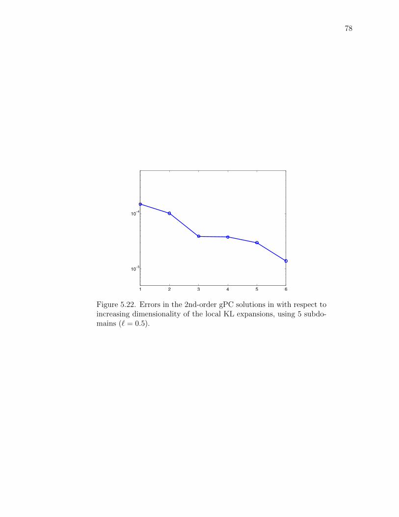
78

1 2 3 4 5 6

10−5

10−4

Figure 5.22. Errors in the 2nd-order gPC solutions in with respect toincreasing dimensionality of the local KL expansions, using 5 subdo-mains (` = 0.5).

79

5.7 Computational Cost

The local gPC method allows a time independent PDE in a global physical do-

main with a high-dimensional random dimension (from the KL-type expansion) to

be decomposed into a set of PDEs in smaller subdomains and with lower random

dimensionality. This can result in substantial computational saving, which is o↵set

by the interface problem (2.33) in the post-processing stage. The interface problem

can be expensive if one uses an exceedingly large number of subdomains.

In fact, the e↵ectiveness of the gPC method is a trade o↵ between the cost of

constructing the local PCE approximations on each subdomain and the cost of solving

the interface problem (2.33). Increasing the number of subdomains decreases the

dimensionality of the local KLE and thus the number of samples required to build

the local gPC approximation. However, increasing the the number of subdomains

requires solving a larger and more computationally expensive interface problem.

Here we present the simulation cost comparison for the two-dimensional example

with correlation length ` = 0.2 from Section 5.3. The global KL expansion results in

d = 94 random dimensions, obtained by retaining all eigenvalues greater than 10�1.

The same truncation tolerance is then used in the local gPC solutions. The FEM

discretization is quadratic elements and in random space we employ the level three

Clenshaw-Curtis stochastic collocation. The computational cost is then estimated

using operational count and demonstrated in Figure 5.23.

We observe that as the number of subdomains increases, the cost for the construc-

tion of the local gPC solutions decreases fast, while the cost for the interface problem

becomes larger. And the solution of the interface problem quickly becomes the dom-

inant cost. Compared against the full FEM solution, we observe at least one order of

magnitude of computational saving, whenever one does not use an exceedingly large

number of subdomains. The comparison is obtained by assuming one generates 106

solution samples. Since both the interface problem and the full FEM solver are based

80

on sampling, the number of samples does not a↵ect the comparison whenever the cost

of interface problem dominates.

We finally remark that the computational cost comparison presented here is pre-

liminary. A complete understanding of e�ciency gain by the local gPC method is

clearly problem dependent. Also, we have not investigated e�cient implementation

of the local gPC method in this first paper. A more comprehensive study of the

computational cost and implementation is the subject of future work.

Figure 5.23. Computational cost in term of operation count versusthe number of subdomains used by the local gPC method for 2 ⇥ 2,4⇥4, 8⇥8, 16⇥16 subdomains, along with the cost by the full globalFEM method.

81

6. SUMMARY

In this work we present a drastically di↵erent method to curb the di�culty posed by

high dimensionality (CoD). The method employs a domain decomposition strategy

so that a potentially high dimensional PDE can be solved locally in each subdomain.

A unique feature of the method is that the local problems in each element are of

very low dimension by local approximation, typically less than five, regardless of the

dimensionality of the random space in original governing equations.

The local subdomain problems are independently defined from each other and with

arbitrarily assigned boundary conditions (typically of Dirichlet type). The solution

of the subdomain problems are then sought in a gPC type by treating the boundary

conditions as auxiliary variables. As long as the gPC solutions in the subdomains are

su�ciently accurate, they allow one to accurately generate solution samples.

A proper coupling algorithm is then applied to each of these samples of the local

solutions at the post-processing stage, where a system of algebraic equations are

solved to ensure the samples satisfy the original governing equations in the global

domain. Applying the surrogate models using independent variables ( [51, 52]) can

indeed reproduce the statistics of the underlying problem via sampling, provided that

the surrogate models are accurate in a strong norm, which is relaxed from L1 norm

in the parameter space ( [51]) to Lp norm, p � 1, in the more recent work of [52].

We extend the previous work [37] and continue to analyze the properties of the

local PCE method. After presenting a brief review of the local PCE method, we

reveal the intrinsic connection between the Schur complement in the tradition DDM

setting and the local PCE method at the interface coupling stage, which characterizes

the local PCE method as a deterministic coupling approach. Besides that, we also

discussed e�cient implementation strageties for the important steps in the local PCE

82

method. This essentially lays a solid foundation for uncertainty quantification for

large scale complex systems in a high dimensional random space.

REFERENCES

83

REFERENCES

[1] N. Wiener. The homogeneous chaos. Amer. J. Math., 60:897–936, 1938.

[2] R.G. Ghanem and P. Spanos. Stochastic Finite Elements: a Spectral Approach.Springer-Verlag, 1991.

[3] D. Xiu and G.E. Karniadakis. The Wiener-Askey polynomial chaos for stochasticdi↵erential equations. SIAM J. Sci. Comput., 24(2):619–644, 2002.

[4] I. Babuska, R. Tempone, and G.E. Zouraris. Galerkin finite element approx-imations of stochastic elliptic di↵erential equations. SIAM J. Numer. Anal.,42:800–825, 2004.

[5] O.G. Ernst, A. Mugler, H.-J. Starklo↵, and E. Ullmann. On the convergence ofgeneralized polynomial chaos expansions. ESAIM: M2AN, 46:317–339, 2012.

[6] P. Frauenfelder, Ch. Schwab, and R.A. Todor. Finite elements for elliptic prob-lems with stochastic coe�cients. Comput. Meth. Appl. Mech. Eng., 194:205–228,2005.

[7] R.G. Ghanem. Ingredients for a general purpose stochastic finite element formu-lation. Comput. Methods Appl. Mech. Engrg., 168:19–34, 1999.

[8] D. Xiu and G.E. Karniadakis. Modeling uncertainty in steady state di↵usionproblems via generalized polynomial chaos. Comput. Methods Appl. Math. En-grg., 191:4927–4948, 2002.

[9] D. Xiu and J. Shen. E�cient stochastic Galerkin methods for random di↵usionequations. J. Comput. Phys., 228:266–281, 2009.

[10] D. Xiu. Numerical methods for stochastic computations. Princeton UniveristyPress, Princeton, New Jersey, 2010.

[11] N. Agarwal and N.R. Aluru. A domain adaptive stochastic collocation approachfor analysis of mems under uncertainties. J. Comput. Phys., 228(20):7662–7688,2009.

[12] B. Ganapathysubramanian and N. Zabaras. Sparse grid collocation methods forstochastic natural convection problems. J. Comput. Phys., 225(1):652–685, 2007.

[13] D. Xiu and J.S. Hesthaven. High-order collocation methods for di↵erential equa-tions with random inputs. SIAM J. Sci. Comput., 27(3):1118–1139, 2005.

[14] F. Nobile, R. Tempone, and C. Webster. An anisotropic sparse grid stochasticcollocation method for elliptic partial di↵erential equations with random inputdata. SIAM J. Numer. Anal., 46(5):2411–2442, 2008.

84

[15] X. Ma and N. Zabaras. An adaptive hierarchical sparse grid collocation algorithmfor the solution of stochastic di↵erential equations. J. Comput. Phys., 228:3084–3113, 2009.

[16] D. Xiu. E�cient collocational approach for parametric uncertainty analysis.Comm. Comput. Phys., 2(2):293–309, 2007.

[17] M. Bieri. A sparse composite collocation finite element method for elliptic sPDEs.Technical Report 2009-08, Seminar for Applied Mathematics, ETHZ, 2009.

[18] M. Bieri and Ch. Schwab. Sparse high order FEM for elliptic sPDEs. Comput.Meth. Appl. Math. Engrg., 198:1149–1170, 2009.

[19] Ch. Schwab and R.A. Todor. Sparse finite elements for elliptic problems withstochastic data. Numer. Math, 95:707–734, 2003.

[20] J. Foo, X. Wan, and G.E. Karniadakis. The multi-element probabilistic collo-cation method (ME-PCM): error analysis and applications. J. Comput. Phys.,227(22):9572–9595, 2008.

[21] X. Wan and G.E. Karniadakis. Multi-element generalized polynomial chaos forarbitrary probability measures. SIAM J. Sci. Comput., 28:901–928, 2006.

[22] X. Wan and G.E. Karniadakis. An adaptive multi-element generalized poly-nomial chaos method for stochastic di↵erential equations. J. Comput. Phys.,209(2):617–642, 2005.

[23] Baskar Ganapathysubramanian and Nicholas Zabaras. Sparse grid collocationschemes for stochastic natural convection problems. Journal of ComputationalPhysics, 225(1):652–685, 2007.

[24] Fabio Nobile, Raul Tempone, and Clayton G Webster. An anisotropic sparsegrid stochastic collocation method for partial di↵erential equations with randominput data. SIAM Journal on Numerical Analysis, 46(5):2411–2442, 2008.

[25] Xiang Ma and Nicholas Zabaras. An adaptive hierarchical sparse grid colloca-tion algorithm for the solution of stochastic di↵erential equations. Journal ofComputational Physics, 228(8):3084–3113, 2009.

[26] Alireza Doostan and Houman Owhadi. A non-adapted sparse approximation ofpdes with stochastic inputs. Journal of Computational Physics, 230(8):3015–3034, 2011.

[27] Liang Yan, Ling Guo, and Dongbin Xiu. Stochastic collocation algorithms usingl 1-minimization. International Journal for Uncertainty Quantification, 2(3),2012.

[28] Xiu Yang and George Em Karniadakis. Reweighted `-1 minimization methodfor stochastic elliptic di↵erential equations. Journal of Computational Physics,248:87–108, 2013.

[29] Xiu Yang, Minseok Choi, Guang Lin, and George Em Karniadakis. Adaptiveanova decomposition of stochastic incompressible and compressible flows. Jour-nal of Computational Physics, 231(4):1587–1614, 2012.

85

[30] Zhen Gao and Jan S Hesthaven. E�cient solution of ordinary di↵erential equa-tions with high-dimensional parametrized uncertainty. Communications in Com-putational Physics, 10(EPFL-ARTICLE-190409):253–278, 2011.

[31] Lijian Jiang, J David Moulton, and Jia Wei. A hybrid hdmr for mixed multi-scale finite element methods with application to flows in random porous media.Multiscale Modeling & Simulation, 12(1):119–151, 2014.

[32] Akil Narayan, Claude Gittelson, and Dongbin Xiu. A stochastic collocationalgorithm with multifidelity models. SIAM Journal on Scientific Computing,36(2):A495–A521, 2014.

[33] Xueyu Zhu, Akil Narayan, and Dongbin Xiu. Computational aspects of stochas-tic collocation with multifidelity models. SIAM/ASA Journal on UncertaintyQuantification, 2(1):444–463, 2014.

[34] Waad Subber. Domain decomposition methods for uncertainty quantification.PhD thesis, Carleton University Ottawa, 2012.

[35] Abhijit Sarkar, Nabil Benabbou, and Roger Ghanem. Domain decomposition ofstochastic pdes: theoretical formulations. International Journal for NumericalMethods in Engineering, 77(5):689–701, 2009.

[36] Qifeng Liao and Karen Willcox. A domain decomposition approach for uncer-tainty analysis. SIAM Journal on Scientific Computing, 37(1):A103–A133, 2015.

[37] D. Venturi H. Cho, X. Yang and G. E. Karniadakis. Numerical methods forpropagating uncertainty across heterogeneous domains. Preprint, 2014.

[38] Yi Chen, John Jakeman, Claude Gittelson, and Dongbin Xiu. Local polynomialchaos expansion for linear di↵erential equations with high dimensional randominputs. SIAM Journal on Scientific Computing, 37(1):A79–A102, 2015.

[39] D. Xiu and G.E. Karniadakis. A new stochastic approach to transient heatconduction modeling with uncertainty. Inter. J. Heat Mass Trans., 46:4681–4693, 2003.

[40] D. Xiu and S.J. Sherwin. Parametric uncertainty analysis of pulse wave propaga-tion in a model of a human arterial networks. J. Comput. Phys., 226:1385–1407,2007.

[41] D. Xiu and G.E. Karniadakis. Supersensitivity due to uncertain boundary con-ditions. Int. J. Numer. Meth. Engng., 61(12):2114–2138, 2004.

[42] Dongbin Xiu and Jan S Hesthaven. High-order collocation methods for di↵er-ential equations with random inputs. SIAM Journal on Scientific Computing,27(3):1118–1139, 2005.

[43] I. Babuska, F. Nobile, and R. Tempone. A stochastic collocation method forelliptic partial di↵erential equations with random input data. SIAM J. Numer.Anal., 45(3):1005–1034, 2007.

[44] S.A. Smolyak. Quadrature and interpolation formulas for tensor products ofcertain classes of functions. Soviet Math. Dokl., 4:240–243, 1963.

86

[45] G.W. Wasilkowski and H. Wozniakowski. Explicit cost bounds of algorithms formultivariate tensor product problems. J. Complexity, 11:1–56, 1995.

[46] H. Engels. Numerical quadrature and cubature. Academic Press Inc, 1980.

[47] V. Barthelmann, E. Novak, and K. Ritter. High dimensional polynomial inter-polation on sparse grid. Adv. Comput. Math., 12:273–288, 1999.

[48] Andrea Toselli and Olof Widlund. Domain decomposition methods: algorithmsand theory, volume 3. Springer, 2005.

[49] John Jakeman, Michael Eldred, and Dongbin Xiu. Numerical approach forquantification of epistemic uncertainty. Journal of Computational Physics,229(12):4648–4663, 2010.

[50] Xiaoxiao Chen, Eun-Jae Park, and Dongbin Xiu. A flexible numerical approachfor quantification of epistemic uncertainty. Journal of Computational Physics,240:211–224, 2013.

[51] J. Jakeman, M. Eldred, and D. Xiu. Numerical approach for quantification ofepistemic uncertainty. J. Comput. Phys., 229:4648–4663, 2010.

[52] X. Chen, E.-J. Park, and D. Xiu. A flexible numerical approach for quantificationof epistemic uncertainty. Journal of Computational Physics, 240(0):211–224,2013.

[53] P.E. Gill, W. Murray, and M.H. Wright. Practical Optimization. Academic Press,London, UK, 1981.

[54] A. Quarteroni and A. Valli. Domain decomposition methods for partial di↵eren-tial equations. Oxford University Press, 1999.

[55] A. Toselli and O. Widlund. Domain decomposition methods – algorithms andtheory. Springer-Verlag, 2010.

[56] Alfio Quarteroni and Alberto Valli. Domain decomposition methods for partialdi↵erential equations numerical mathematics and scientific computation. OxfordUniversity Press New York, 1999.

[57] George Karniadakis and Spencer Sherwin. Spectral/hp element methods for com-putational fluid dynamics. Oxford University Press, 2005.

[58] V. Barthelmann, E. Novak, and K. Ritter. High dimensional polynomial inter-polation on sparse grids. Advances in Computational Mathematics, 12:273–288,2000.

[59] F. Nobile, R. Tempone, and C. G. Webster. A sparse grid stochastic collocationmethod for partial di↵erential equations with random input data. SIAM Journalon Numerical Analysis, 46(5):2309–2345, January 2008.

[60] G.T. Buzzard. E�cient basis change for sparse-grid interpolating polynomialswith application to T-cell sensitivity analysis. Computational Biology Journal,2013, April 2013.

87

VITA

Yi Chen was born on April 20th, 1987 in China. He received his B.S. degree of

mathematics and applied mathematics in 2009 at Zhejiang University. From 2010,

he started to work under Professor Dongbin Xiu0s supervision towards the Ph.D.

degree in applied mathematics at Purdue University. For a detailed vita please go to

http://www.math.purdue.edu/⇠chen411.

Local polynomial chaos expansion method for high ...

Documents

Transcript of Local polynomial chaos expansion method for high ...