Journal of Educational MeasurementFall 2011, Vol. 48, No. 3, pp. 229–254

Local Linear Observed-Score Equating

Marie WibergUmea University

Wim J. van der LindenCTB/McGraw-Hill

Two methods of local linear observed-score equating for use with anchor-test andsingle-group designs are introduced. In an empirical study, the two methods werecompared with the current traditional linear methods for observed-score equating.As a criterion, the bias in the equated scores relative to true equating based onLord’s (1980) definition of equity was used. The local method for the anchor-testdesign yielded minimum bias, even for considerable variation of the relative diffi-culties of the two test forms and the length of the anchor test. Among the traditionalmethods, the method of chain equating performed best. The local method for single-group designs yielded equated scores with bias comparable to the traditional meth-ods. This method, however, appears to be of theoretical interest because it forces usto rethink the relationship between score equating and regression.

The goal of observed-score equating is to adjust the number-correct scores on anew test form to make them indistinguishable from the scores on an old form. Thechoice of equating procedure to realize this goal depends on the sampling design forthe observed scores on the two forms.

The three basic designs for equating studies are: (1) the single-group (SG) design,which consists of a single sample of test takers taking both forms; (2) the equivalent-groups (EG) design, which consists of two random samples of test takers from thesame population both taking a different form; and (3) the nonequivalent-groups-with-anchor-test (NEAT) design, which consists of two groups randomly sampled fromdifferent populations both taking a different form along with some common items.More detailed descriptions of these equating designs are given in Kolen and Brennan(2004) and von Davier, Holland, and Thayer (2004a).

In the NEAT design, the common items can be a subset of items serving as aninternal anchor to the two forms or a separate external anchor test. For notationalconvenience, we assume an external anchor test throughout this paper. But, as forthe statistical nature of the equating procedure, it is irrelevant whether the anchor isinternal or external. We will return to this point later. More importantly, however, nomatter the position of the anchor, in this context it should be long enough to provideaccurate information and its content specifications should match those of the twoforms that are to be equated. Both conditions lead to higher correlations between thescores on the anchor items and the two test forms, and higher correlations alwaysmean a better anchor test (von Davier, Holland, & Thayer, 2004a).

The equipercentile equating transformation maps the observed-score populationdistribution on one test form onto the distribution on the other. The use of the

Copyright c© 2011 by the National Council on Measurement in Education 229

Wiberg and van der Linden

transformation is not unique to test equating; the transformation actually is the Q-Q transformation used in statistics as a general statistical tool for matching differentdistributions (Wilk & Gnanadesikan, 1968). To define the transformation, we denotethe observed scores on the new and old test forms by X and Y and use FY (y) andFX (x) to denote their (cumulative) distribution functions. We will also use the Latincapitals X and Y to denote the test forms themselves. For simplicity, it is assumed thatthe two functions are continuous and strictly increasing. The equipercentile equatingtransformation is then defined as

x = ϕ(y) = F−1X (FY (y)). (1)

If the equating is to be linear, only the mean and variance of the two distributionsare matched. Let μY and μX be the observed-score means of Y and X , respectively,and σY and σX their standard deviations. The linear equating transformation from Yto X is defined as (Kolen & Brennan, 2004)

x = ϕ(y) = μX + σX

σY(y − μY ). (2)

The equation only specifies the general shape of the transformation. For differentequating designs, the two sets of means and standard deviations in it have to beinferred from actual test scores using different sets of assumptions.

Linear equating can be viewed as an approximation to equipercentile equatingbased on the first two moments of the observed-score distributions. (Interestingly, itcan also be viewed as a limiting case of kernel smoothing of the distributions withthe bandwidth parameters approaching infinity; for this perspective, see von Davier,Holland, & Thayer, 2004a) One may wonder why we should ever use a linear ap-proximation and not always prefer equipercentile equating based on the full distribu-tions. However, this choice would be statistically naive. Unless we have extremelylarge samples, estimates of observed-score distributions are notoriously inaccurate,particularly with respect to their tails when the number of score points increases.On the other hand, for equal sample sizes, estimates of means and variances havemuch higher accuracy. As a consequence, the choice between linear and equiper-centile equating faces the well-known trade-off between bias and accuracy that ex-ists throughout statistics. If the bias due to the assumption of linearity is minor (thatis, when the two score distributions do not differ too much in their higher moments,especially their skew), it is generally prudent to accept the bias as a small price fora much more favorable mean square error relative to equipercentile equating. A dis-cussion of the practical cases in which linear and equipercentile equating are mostappropriate can be found in Kolen and Brennan (2004; see especially their Table8.5).

This research was motivated by some persistent problems in traditional observed-score equating and in particular by the difficulty in realizing the requirements ofequity and population independence. Lord’s equity requirement stipulates that eachconditional distribution of the equated scores given the ability measured by the tests

230

Local Linear Equating

should be identical to the conditional distribution of the scores to which the equatingoccurs. For a common ability θ measured by X and Y , it can be formulated as (Lord,1980):

Fϕ(Y )|θ = FX |θ , (3)

for all θ. If the requirement holds, the equated scores are indistinguishable from thescores to which they are equated.

van der Linden (2000) showed that Lord’s criterion of equity actually implies afamily of equating transformations with a different member for each ability level.The family follows directly from (3) using the equipercentile transformation to mapthe conditional rather than the marginal distributions of Y onto those of X; that is, as

ϕ∗(y; θ) = F−1X |θ (FY |θ (y)), θ ∈ R. (4)

The necessity of an entire family of transformations reveals a serious flaw in thetraditional methods which all assume a single transformation for some populationof test takers. As a single transformation for an entire population necessarily hasto compromise between what should be used at different ability levels, it producesequated scores for the individual test takers that are always biased. In addition, asthe nature of the compromise depends on the shape of the ability distribution inthe chosen population of test takers, the equated scores are necessarily populationdependent.

This research is part of a program that tries to use the family of the true equatingtransformations in (4) to (i) define equating error, study equating bias, and otherwiseevaluate the traditional equating methods, and (ii) find new equating methods thatoffer better approximation to the true transformations and consequently minimizeequating bias and population dependency. Because of the attempt to approximate theindividual members of the family of transformations as closely as possible using allempirical information about the test taker’s ability available in the equating design,we refer to this new type of equating as “local equating” (van der Linden, 2000,2006a, 2011).

The focus of the current research is on linear equating. Two local methods forthis type of equating were derived and their properties were compared with the ma-jor traditional linear methods. In addition, all methods were evaluated against thetrue equating transformations using the simulated observed scores for which thesetransformations were known.

Linear Equating Methods

As already noted, the main differences between the traditional equating meth-ods for the three different data-collection designs exist in the way the populationmeans and standard deviations in the linear transformation in (1) are estimated fromthe test scores. For the SG and EG designs, the estimation is straightforward, but

231

Wiberg and van der Linden

for the NEAT design several possibilities are available, each relying on differentstatistical assumptions. We will review the assumptions for the Tucker, Levine,chain linear equating, and Braun-Holland methods. For more in-depth introductionsto these methods, see Braun and Holland (1982), Kolen and Brennan (2004), vonDavier, Holland, and Thayer (2004a), or von Davier and Kong (2005).

Each of these methods (except chain linear equating) relies on the notion of asynthetic population, i.e., a new population S that is a weighted combination of thepopulations P and Q that take X and Y , respectively. The synthetic population issymbolically defined as S = w1 P + (1 − w2)Q, with w1and w2 weights satisfyingthe constraint w1 + w2 = 1 (Braun & Holland, 1982). Setting the weights equal,i.e., w = w1 = w2 = .5, reflects the case of both populations being considered asequally important (Kolen & Brennan, 2004). The linear equating transformation forthis synthetic population is defined as

x = ϕ(y) = μS(X ) + σS(X )

σS(Y )(y − μS(Y )); (5)

that is, with the means and standard deviations for the two forms estimated from Sinstead of P and Q.

Tucker Method

The Tucker method is based on the following assumptions: (i) the regressions ofX and Y on the anchor score A are the same linear functions in populations P andQ, and (ii) the conditional variances of X and Y given A are the same for bothpopulations (Braun & Holland, 1982; Kolen & Brennan, 2004; von Davier & Kong,2005).

Using these assumptions, the means and standard deviations in (5) can be derivedas

μS(X ) = μP (X ) − wQγP (μP (A) − μQ(A)), (6)

μS(Y ) = μQ(Y ) − wPγQ(μP (A) − μQ(A)), (7)

σ2S(X ) = σ2

P (X ) − wQγ2P (σ2

P (A) − σ2Q(A)) + wPwQγ2

P (μP (A) − μQ(A))2, (8)

σ2S(Y ) = σ2

Q(Y ) − wPγ2Q(σ2

P (A) − σ2Q(A)) + wPwQγ2

Q(μP (A) − μQ(A))2, (9)

with γP and γQ regression slopes defined by

γP = σ2P (X , A)/σ2

P (A), (10)

γQ = σ2Q(Y , A)/σ2

Q(A). (11)

232

Local Linear Equating

Plugging the sample equivalents of these parameters into (5), an estimate of theTucker linear equating transformation is obtained.

It should be noted that the Tucker method relaxes the usual assumption ofpopulation-invariant conditional distributions of X and Y given A = a to the oneof invariant regressions of X and Y on A. In addition, it requires the residual vari-ances to be constant (Braun & Holland, 1982; Kolen & Brennan, 2004).

Levine Method

The Levine method for observed-score equating relies on the assumptions of theclassical test theory model for all three observed scores. For a fixed test taker, themodel can be represented as

X = τX + EX , (12)

Y = τY + EY , (13)

A = τA + E A, (14)

where τX , τY , and τA are the true scores defined as the expected values of X, Y, andA across replicated administrations of the test to the test taker, respectively. EX , EY ,

and E A are the errors defined as the differences between the observed and true scoresacross the replications. It follows from these definitions that the errors have expecta-tions equal to zero and they do not correlate with the true scores in any population oftest takers.

In addition, it is assumed that (i) true scores TX , TY , and TA correlate perfectlyin populations P and Q, (ii) the regressions of TX and TY on TA are the same linearfunction for both populations, and (iii) the measurement errors EX , EY , and E A areidentically distributed in both populations (Kolen & Brennan, 2004; von Davier &Kong, 2005). Basically, these assumptions formalize the more intuitive requirementof X, Y , and A “measuring the same variable equally well.”

From these assumptions, it follows that the means and variances of the syntheticpopulation are the same as for the Tucker method but with the regression slopes in(10) and (11) replaced by

γP = σP (TX )/σP (TA), (15)

γQ = σQ(TY )/σQ(TA). (16)

The slopes in (15) and (16) are defined for unobservable true scores. However,they can be expressed as functions of observed variables,

γP = σP (X )√

ρP (X , X ′)σP (A)

√ρP (A, A′)

, (17)

233

Wiberg and van der Linden

γQ = σQ(Y )√

ρQ(Y , Y ′)

σQ(A)√

ρQ(A, A′), (18)

and estimated using one of the standard methods for estimating the reliabilitycoefficients ρP (X , X ′), ρQ(Y , Y ′), ρQ(A, A′), and ρP (A, A′) (Kolen & Brennan,2004).

Braun-Holland Method

Braun and Holland (1982) proposed a linear method similar to the Tucker method.In fact, the method becomes identical to Tucker linear equating when the regressionsof X on A and Y on A are both linear and homoscedastic (Braun & Holland, 1982;Kolen & Brennan, 2004). The means and standard deviations can then be defined as

μS(X ) =∑

x

x fs(x), (19)

μS(Y ) =∑

y

y fs(y), (20)

σ2S(X ) =

∑x

[x − μS(X )]2 fs(x), (21)

σ2S(Y ) =

∑y

[y − μS(Y )]2 fs(y). (22)

Substitution of the sample equivalents of (19)–(22) into (5) yields the equatingtransformation. The Braun-Holland method is claimed to be useful when the re-gressions of X and Y on the anchor-test score A are nonlinear (Kolen & Brennan,2004).

Linear Chain Equating

An alternative to these poststratification methods for NEAT designs is chain equat-ing. The basic idea of chain equating is to equate Y to the anchor-test score A forpopulation Q and then equate A to X for population P . The two equating transfor-mations are then combined or “chained” together (Kolen & Brennan, 2004). For thecombination of two linear transformations, the result is

x = ϕ(y) = μPX + σP

X

σPA

(μQA − μP

A) + σPX

σQY

σQA

σPA

(y − μQY ). (23)

234

Local Linear Equating

Linear chain equating is based on the assumptions of population invariance withrespect to the two basic linear transformations functions from Y to A and from A toX (von Davier, Holland, & Thayer, 2004b; von Davier & Kong, 2005).

Local Equating

As described in Lord (1980), equating methods should satisfy the three fundamen-tal criteria of (i) equity, (ii) population independence, and (iii) symmetry. Besides,of course, test scores should only be equated when they measure the same construct.For a discussion of these criteria, see Kolen and Brennan (2004).

As already observed, the criteria of equity and population independence are themost challenging ones. The linear equating methods reviewed above ignore the crite-rion of equity. Besides, they simply assume the criterion of population independenceto hold, not offering anything to check on it. Also, with the exception of the methodof chain equating, they rely heavily on the notion of a synthetic population whichcreates a mismatch between the population for which the equating transformation isderived and the test takers for which it is actually used (van der Linden & Wiberg,2010).

Methods of local equating deal directly with the criteria of equity and populationindependence. They can be motivated from different points of view. One motivationis that a single transformation can never yield equitable equatings because it alwayshas to compromise between the score distributions of different test takers. The onlyway to reduce the bias is to abandon the idea of a “one-size-fits-all” score transfor-mation and replace it with a family of transformations with different members foreach ability level. In an actual equating, we then pick the member from the familythat is best given what we know about the test taker’s ability.

This argument, which was already used briefly in the introductory section of thispaper, is not further pursued here; readers interested in details should consult vander Linden (2006a, 2006b, 2011) or van der Linden and Wiberg (2010). Instead, weuse the notions of matching and conditioning to motivate the idea of local equating.Both notions have popped up earlier in the equating literature (e.g., Cook & Petersen,1987; Dorans, 1990; Liou, Cheng, & Li, 2001; Livingston, Dorans, & Wright, 1990;Wright & Dorans, 1993) but have only been exploited to adjust a population distri-bution for use with a single equating transformation (that is, as an alternative to thesynthetic population discussed earlier). Here, we use the same notions to motivate theuse of a family of transformations to deal with the criteria of equity and populationindependence.

Matching is a standard technique for creating groups of subjects comparable onone or more relevant variables. In the context of observed-score equating, matchingon a variable results in different pairs of distributions of the observed scores X andY for each value of the matching variable. Or, in distributional language, when testtakers are matched on a variable, the focus moves from the marginal populationdistributions of X and Y to their conditional distributions given the values of thematching variable.

If we match or condition on information on the test taker’s ability, the resulthas the potential of improving observed-score equating in important respects. First,

235

Wiberg and van der Linden

because we condition on ability information, the equating becomes less dependent onthe ability distribution in the population of test takers that is considered. The more ac-curate the information, the stronger the effect. In the limit, if we condition on the trueability of the test taker, the equating becomes completely population-independent.

Second, the conditional distributions of X and Y approximate the observed-scoredistributions of the individual test takers. Again, if we could condition on the trueability, the conditional distributions would become the test taker’s observed-scoredistributions on X and Y and we could use (4) for the equating with a result thatwould perfectly meet Lord’s criterion of equity. Also, as we no longer compromisedbetween what is required for different ability levels, the bias in the equatings woulddisappear.

The argument shows how closely related the problems of inequity, population de-pendence, and bias in observed-score equating are. Each of them has the same causeof the equating being based on a single transformation derived from the marginaldistributions of X and Y for a population of test takers. The same fact was alluded toby Dorans and Holland (2000, p. 384) when they noticed that “a single linking func-tion is inappropriate when population invariance fails to hold to a sufficient degree.”However, rather than their general recommendation to use “several different . . .

functions for important subpopulations,” our analyses show that the only way toreduce these problems is to use different functions for subpopulations defined by thesame ability level. Or, in more practical terms, we must use all information aboutthe ability available in the equating study as a conditioning variable and equate theobserved scores using the distributions conditional on the variable. This is exactlywhat local equating tries to achieve.

We consider Lord’s third equating criterion of symmetry as less important thanequity and population independence. The main purpose of using the criterion in theequating literature has been to rule out linear regression as an equating method (e.g.,Kolen & Brennan, 2004). But if a method can be proven to be less biased by sacri-ficing some of its symmetry, there are strong statistical arguments for doing so (vander Linden, 2011). In fact, the Tucker and Braun-Holland methods above as well asthe traditional equipercentile method are only symmetric when their synthetic popu-lation weights are equal (that is, w1 = w2 = .5). The local linear anchor-test methodpresented below is symmetric in x and y given the anchor-test score A = a but themethod of conditional means is not. Both methods will be evaluated for their biasagainst the traditional linear methods.

Use of Proxies for Ability

From a practical perspective, an important question is, what information aboutthe common ability measured by the test forms should be used to approximate theconditional distributions required for the true equating transformations in (4)? Oneobvious answer is to use the extra information in the vector of responses by the testtaker above and beyond simple number-correct scoring. This information is presentfor any type of equating design. If the two test forms fit a common IRT model, wecan simply use the true transformations in (4) with an estimate of θ substituted for thetrue ability. For applications of this local method with excellent results, see Janssen,

236

Local Linear Equating

Magis, San Martin, and Del Pino (2009) and van der Linden (2000, 2006a, 2006b).Our current intention, however, is to avoid any assumption beyond the classical testtheory model from which some of the earlier traditional equating methods have bor-rowed assumptions.

A key notion in our derivation of two new equating methods is one of a proxy forthe common ability measured by the two forms. A proxy is defined as any monotonefunction of the ability that is measured. As the proxy will be used only as a condition-ing variable, the function does not need to be known. A statistical estimator, such asthe maximum-likelihood estimate (MLE) of θ in a response model fitting the items,is definitely a good proxy. But a good proxy does not need to be a good estimatorbecause it cannot be on a scale different from θ.

More formally, let P be a proxy that is considered. Analogous to (12)–(14), thetest taker’s true score for P is defined as

τP = E(P). (24)

For P to be a valid proxy, its true score should be a strictly monotonically in-creasing function of the ability θ measured by the two forms. It should thus holdthat

τP = g(θ), (25)

where g can be any monotone function. Observe that the assumption does not implylinear correlation between the true scores TX , TY , and TA, only that these scores aremonotonically related. The assumption is thus weaker than the one of perfect linearcorrelation for the Levine method.

Local equating is based on the conditional distribution functions FX |θ.(x) andFY |θ.(y). However, these distributions are identical to those of X and Y given τP.The truth of the claim follows directly from (25). Because of the monotonicity, theinverse function θ = g−1(τP) exists. Therefore,

FX |θ (x) = FX|g−1(τP ) (x) = FX |τP (x), (26)

and likewise,

FY |θ (y) = FY |τP (y). (27)

Thus, all we need to do to approximate the required conditional distributionsFX |θ.(x) and FY |θ.(y) is to find an accurate proxy P with the (strict) monotonic rela-tionship in (25) and condition the observed scores X and Y on it. The function itselfcan remain unknown; the fact that P and θ are on different scales does not matter.

The quality of the approximation depends solely on the reliability of P. The effectof less than perfect reliability is the use of a mixture of the conditional distributionsFX |θ.(x) and FY |θ.(y) over the distribution of θ given the observed value P = p for theproxy rather than the exact distributions we need. The more reliable the proxy, thenarrower the mixing distribution and the better the result.

237

Wiberg and van der Linden

But even for a less reliable proxy, the gain relative to traditional equating is alreadysubstantial. The best way to view this is by observing the differences between thefollowing pairs of conditional distributions: The distributions that should be used toequate X and Y are FX |θ.(x) and FY |θ.(y) in (4). If we condition on a proxy for θ, thedistributions we actually use are

∫FX |θ (x) f (θ |p )dθ and

∫FY |θ (y) f (θ |p )dθ. (28)

In traditional equating, the distributions used to derive the equating transformationare

∫FX |θ (x) f (θ)dθ and

∫FY |θ (y) f (θ)dθ, (29)

with f (θ) the ability distribution of the entire (synthetic) population that is consid-ered.

The gain in the use of P as a proxy is due to the fact that f (θ|p) can be expectedto be a considerably narrower mixing distribution than f (θ). For a perfectly reliableproxy, f (θ|p) becomes a point distribution at the test taker’s true ability and the equat-ing will be fully equitable and population-independent.

It is straightforward to derive quantitative measures of the relative qualities oftraditional equating and proxy-based local equating from the expressions in (28) and(29). But such measures are beyond the scope of this paper.

Two Methods of Local Linear Equating

In the following sections, we present two different families of linear transforma-tions for observed-score equating and discuss their features. The first family is for theNEAT design; the second for is the SG design. Both families are based on a differentchoice of proxy.

Local Linear Anchor-Test Method

For the NEAT design, a linear version of the local equating method in van derLinden and Wiberg (2010) is proposed. The method is based on the choice of theanchor score A as a proxy of the ability measured by X and Y—a choice that makessense given that anchor tests should be built according to the same specificationsas the test forms that are equated. Under this condition, the assumption of the trueanchor score being a monotonically increasing function of the ability measured bythe two forms seems trivial. Finally, as the focus is on linear equating, the differencesbetween the conditional distributions of X and Y given A = a are assumed to bedescribed satisfactorily by their first two moments.

The assumptions result in the family of local linear transformations

x = ϕa(y) = μX |a + σX |aσY |a

(y − μY |a), a ∈ {0, 1, . . . , m}, (30)

238

Local Linear Equating

with anchor-test score a serving as the index of the family (i.e., identifier of itsmembers).

The family differs from the traditional transformation in (2) because of the useof the first two moments of the conditional distributions of X and Y given A = ainstead of their marginal moments. Besides, except for linearity, it differs from thetrue family in (4) in that its members are indexed by the anchor score a instead of θ.In the unlikely case of a sufficiently large sample for which one of the scores on Anevertheless has zero frequency, we should interpolate the equated scores just as fortraditional equipercentile equating (for the method of linear interpolation, see Kolen& Brennan, 2004, sect. 2.5).

It is interesting to compare the current assumptions about the anchor test withthose for the Tucker, Levine, and Braun-Holland methods of linear equating. Theassumptions for the latter are necessary to adjust the estimates of the marginal meansand standard deviations in (2) for the differences between the ability distributions inthe two populations P and Q or to derive a synthetic population as a compromisebetween the two. For the local method, there is neither a need to adjust for populationdifferences nor to introduce a synthetic population. Whatever population a test takermay belong to, we just condition the two test scores on the anchor score assumed tobe the proxy for the ability measured by the test.

Method of Conditional Means

The SG design is the only type of design that gives an estimate of the joint dis-tribution of the observed scores on X and Y . The second method capitalizes on thisfact.

Obviously, the score on the new test form, Y , measures the intended ability of thetest takers. The assumption of its true score τY meeting the monotonicity conditionin (25) thus should be automatically met. So, it is tempting to explore the use ofthe observed score Y = y on the new form as a proxy and base the equating on theconditional distributions of X and Y given the observed score on form Y . We doso primarily for theoretical reasons, not because we expect immediate convincingsuccess. The reasons for our motivation will become clear below.

If we condition on Y = y, the linear transformation in (1) results in the family oftransformations

x = ϕy(y) = μX |y + σX |yσY |y

(y − μY |y) , y ∈ {0, . . . , n}, (31)

with index y.The conditional distribution of X given Y = y can be estimated directly from the

joint distribution of X and Y sampled in the SG design. The estimation of μX |y andσX |y is thus straightforward.

The distribution of Y given y is the observed-score distribution of Y that would beobtained if we replicated the administration of Y for all test takers with the currentscore Y = y. The distribution is not directly accessible. But surprisingly for linear

239

Wiberg and van der Linden

equating it is unnecessary to know it. From classical test theory, it follows that

μY |y = y. (32)

Consequently, substitution of y for μY |y. simplifies the family in (31) to

x = ϕy(y) = μX |y , y ∈ {0, . . . , n}. (33)

The simple result can be summarized by stating that local linear equating for theSG design with just the score on the new form as proxy involves the assignment ofthe conditional mean μX |y. to each score y on form Y . The conditional variances σ2

X |yand σ2

Y |y do not play any role.It may seem as if the choice of the proxy in this method confounds the use of

the test scores on the new form as a conditioning variable with the score that isequated. In fact, this would be the case if these scores were fixed values. However,in classical test theory only the true score for each individual test taker is fixed;observed scores are random because of measurement error. Therefore, conditioningon Y = y is a meaningful operation; practically, it means pooling all test takers withthe same realized observed score Y = y but with different measurement errors. Ifthere were no measurement error, Y would be a fixed value for each test taker andeach replication of Y would result in the same observed score. Only in this ideal casewould we condition on the score that is to be equated.

Also, use of the method of conditional means should not be confused with a directpostulate of the use of the regression function for the equating. The family in (33) isa special case of the linear family in (31) due to the fact that classical measurementerror has zero expectation across replications.

Observe that the standard warning in the traditional equating literature againstthe confusion between a linear equating transformation and a regression line (e.g.,Kolen & Brennan, 2004) does not apply here—our result is a regression function,not a regression line. Nevertheless, the formal equivalence between the current formof linear equating and regression is intriguing. Apparently, as soon as we allow formeasurement error the standard warning may no longer apply and we have to rethinkthe relationship between score equating and (nonlinear) regression.

Internal Anchoring

The only relevant difference between an internal and external anchor is the in-clusion of the anchor items in the test scores. The adjustment to internal anchorsrequired for the local method in (30) is minimal. Let Xu and Y u denote the number-correct scores on the unique items in X and Y . The total scores on the two formsare equal to X = Xu+A and Y = Y u+A. Both score components can be taken tobe independent (assumption of “local independence”). The anchor-score componentneed not be equated. Thus, for the local anchor-test method, we can just equate Y u

to Xu given A = a and add anchor score a to the result. More formally, the family of

240

Local Linear Equating

transformation in (30) needs to be adjusted as

x = ϕa(y) = μXu |a + σXu |aσYu |a

(yu − μYu |a) + a, a ∈ A. (34)

The method of conditional means does not assume any anchor items. But if thetwo test forms would happen to have them, we should adjust (12) analogously as

x = ϕy(y) = μXu |yu + a , y ∈ {0, . . . , n}. (35)

Empirical Study

The goal of this part of the study was empirical evaluation of the traditional andlocal methods of linear equating discussed in this paper. As we wanted to evaluatethese methods for bias in their equatings, the true equating transformations mappingthe distributions of the observed scores on Y on the distributions for the scores on Xhad to be known. The evaluation thus only was possible using simulated test scores.

The test scores on the two test forms were simulated under the 3-parameter logistic(3PL) response model. As both the ability of each simulated test taker and the itemparameters in the test forms were known, we knew the conditional distributions of theobserved number-correct scores X and Y given θ. The distributions are generalizedbinomial, with distribution functions FX |θ(x) and FY |θ(y) that can be calculated usingthe recursive algorithm in Lord and Wingersky (1984). The true equating transfor-mations x = ϕ∗(y) in (4) were calculated directly from these distribution functions.

The decision to generate the data under the 3PL model restricts the generalityof our conclusions below. However, the model is one of the most commonly usedmodels for unidimensional tests in the testing industry—unidimensionality being anassumption that has to be satisfied for any observed-score equating to be meaning-ful. For items with other than a dichotomous response format, the study should berepeated with a response model appropriate for the format.

The bias of each of the methods in this research was examined by comparing thepertinent transformation x = ϕ(y) with the corresponding true transformation x =ϕ∗(y) in (4). Using,

bias(ϕ(y); θ) = ϕ(y) − ϕ∗(y; θ) , θ ∈ R. (36)

Since Y and A are random, the local anchor-test method and the method of con-ditional means had to be evaluated by taking the expectations over Y and A given θ

across the simulated replications. Thus,

bias(ϕY (y); θ) = EY |θ[ϕY (y) − ϕ∗(y; θ)] , θ ∈ R, (37)

bias(ϕA(y); θ) = E A|θ[ϕA(y) − ϕ∗(y; θ)] , θ ∈ R. (38)

241

Wiberg and van der Linden

The main factor varied in this study was the difficulty of form Y relative to X .In addition, to assess the price of economizing on the anchor-test design, we alsoexplored how far the length of the anchor test could be shortened before yieldingunsatisfactory results.

It should be noted that, for the current case of linear equating with realisticobserved-score distributions, the bias measures in (36)–(38) capture both (i) the ear-lier bias due to population dependency (traditional methods) or conditioning on animperfect proxy (local methods) and (ii) the assumed linearity of the transformation.The latter would disappear only when all (conditional) observed-score distributionsdiffered only in their first two moments. However, a comparison with the results invan der Linden and Wiberg (2010) allows us to assess the effect of the linearity as-sumption for some of the methods. These authors studied poststratification and chainequating for the NEAT design using exactly the same test forms and sampling fromthe same populations as in our examples. The Tucker, Levine, and Braun-Hollandtransformations are linear versions of the equipercentile transformation used in post-stratification equating. The same relationship exists between the local anchor-testmethods in van der Linden and Wiberg (2010) and this research. The method ofthe conditional means has no nonlinear equivalent, and its bias due to the assumedlinearity therefore remains unknown.

Method

The methods were evaluated for the equating of one test form assembled from anitem pool from the Law School Admission Test (LSAT) to another test form. Forthe anchor-test design, a third form from the same pool was used as the anchor. Thethree test forms were randomly sampled from the item pool and each had a lengthof m = 40 items. The actual LSAT is longer but the current test length was chosento fit the earlier empirical studies with an anchor test size between 20 and 60 items(e.g., Kolen & Brennan, 2004, p. 271; Petersen, Marco, & Stewart, 1982; von Davier,Holland, & Thayer, 2004a, p. 156).

The number-correct scores on each of the test forms were generated for N =50,000 test takers. This large sample size is not a requirement for linear equating. Itwas chosen here because the interest was in an estimate of the bias in the equatingmethods and we did not want to confound our bias estimates with the accuracy ofthe methods. For the SG design, the test takers were sampled from N (0, 1). For theNEAT design, the test takers were sampled randomly from N (−.5, 1) for populationP and N (.5, 1) for population Q. The Tucker, Levine, and Braun-Holland methodswere used with weight w = .5—a choice usually defended as representing the caseof two equally relevant populations (Kolen & Brennan, 2004). The conditional dis-tribution functions FX |θ and FY |θ necessary for the true transformation in (4) werecalculated at θ = −2.0, −1.9, ..., 2.0. The transformations at these values were ob-tained using equipercentile equating with simple linear interpolation to deal with thediscreteness of the scores (Kolen & Brennan, 2004). The bias in the equating trans-formations was evaluated at the θ value closest to the test taker’s sampled true valueof θ.

Several of the bias functions in the figures below do not run over the whole rangeof possible values of y due to the fact that we have omitted all results for the values

242

Table 1Descriptive Statistics for the Test Forms Used in the Simulation Study

Design Test Form Mean SD A rXA

SGX 23.13 5.88 .75 –Y 20.00 5.20 .66 –

Y (more difficult) 17.97 4.96 .63 –Y (less difficult) 22.14 5.33 .68 –

NEATX 20.60 5.77 .73 –Y 22.12 5.32 .68 –

Y (more difficult) 19.97 5.18 .66 –Y (less difficult) 24.34 5.32 .69 –A (population P) 19.92 5.33 .69 .71A (population Q) 24.49 5.42 .72 .70

of Y with a probability lower than 10−4 because their equatings would have beentoo unstable. This choice does not have any consequences; in practical applications,only a few test takers would obtain one of the omitted values, and their equated scoresshould never be reported without a warning about their lack of accuracy.

Test forms X and Y had an average difficulty parameter equal to .08 and .71, re-spectively. In the conditions with a more or less difficult form Y , the value of .5 wasadded to or subtracted from its difficulty parameters, not changing the parameters ofform X. These changes in the difficulty of Y are extreme, especially given the factthat Y was already more difficult. But our only goal was to illustrate the possible im-pact of a large inequality in item difficulty on score equating as clearly as possible.The effect of the length of the anchor test was examined by shortening the baselinecase of m = 40 to m = 30 and m = 20 items. The test was shortened by randomlyremoving items. As a result, the alternative anchor tests had average item difficultiesb40 = .13, b30 = –.02, and b20 = .03, respectively.

Table 1 summarizes the properties of all three test forms for each of the conditionsin this study. The statistics show enough variation in the mean, standard deviation,and Cronbach’s α between the forms to challenge our score equating. The correla-tions between the test forms and the anchor test for the NEAT design were of thesame order as their estimated reliabilities.

Results

For clarity, only the results for θ = −2.0, −1.0, 0, 1.0, and 2.0 are shown. Forthe same reason, for the local anchor-test method only the results for every otherobserved score on the anchor test are displayed. However, all omitted results fit thegeneral pattern in these figures.

Figures 1 and 2 show the results for the baseline case. As in all other figures,the true transformations are generally ordered with respect to their θ values. TheTucker, Levine, Braun-Holland, and chain equating methods have one equating

243

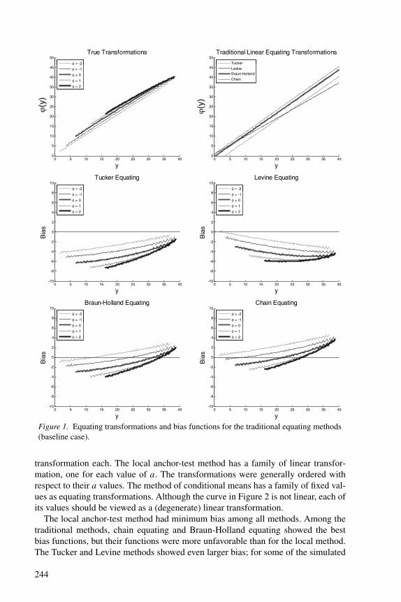
Figure 1. Equating transformations and bias functions for the traditional equating methods(baseline case).

transformation each. The local anchor-test method has a family of linear transfor-mation, one for each value of a. The transformations were generally ordered withrespect to their a values. The method of conditional means has a family of fixed val-ues as equating transformations. Although the curve in Figure 2 is not linear, each ofits values should be viewed as a (degenerate) linear transformation.

The local anchor-test method had minimum bias among all methods. Among thetraditional methods, chain equating and Braun-Holland equating showed the bestbias functions, but their functions were more unfavorable than for the local method.The Tucker and Levine methods showed even larger bias; for some of the simulated

244

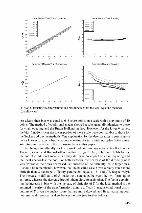
Figure 2. Equating transformations and bias functions for the local equating methods(baseline case).

test takers, their bias was equal to 6–8 score points on a scale with a maximum of 40points. The method of conditional means showed results generally identical to thosefor chain equating and the Braun-Holland method. However, for the lower θ values,the bias functions over the lower portion of the y scale were comparable to those forthe Tucker and Levine methods. One explanation for the deterioration is guessing—afactor known to affect observed-score equating for tests with multiple-choice items.We return to this issue in the discussion later in this paper.

The changes in difficulty for test form Y did not have any noticeable effect on theTucker, Levine, and Braun-Holland methods (Figures 3–6). The same holds for themethod of conditional means. But they did have an impact on chain equating andthe local anchor-test method. For both methods, the decrease of the difficulty of Ywas favorable: their bias decreased. But increase of the difficulty led to larger bias.It should be remembered, however, that the baseline case Y was already much moredifficult than X (average difficulty parameters equal to .71 and .08, respectively).The increase in difficulty of .5 made the discrepancy between the two forms quiteextreme, whereas the decrease brought them close to each other. The factor explain-ing the increase in bias with the increase of difficulty of Y for the local method is theassumed linearity of the transformation: a more difficult Y means conditional distri-butions of Y given the anchor score that are more skewed, and linear equating doesnot remove differences in skew between scores (see further below).

245

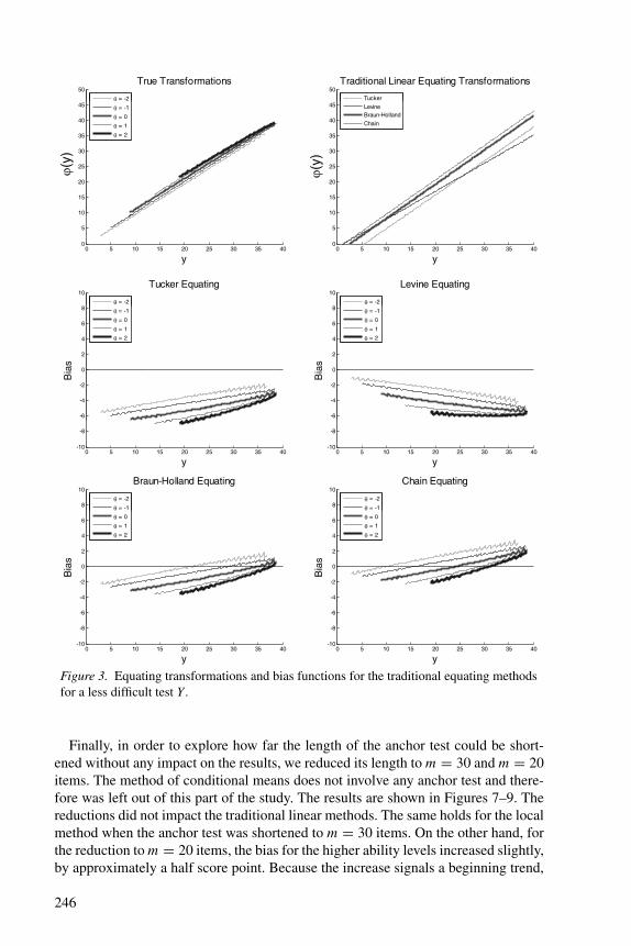
Figure 3. Equating transformations and bias functions for the traditional equating methodsfor a less difficult test Y .

Finally, in order to explore how far the length of the anchor test could be short-ened without any impact on the results, we reduced its length to m = 30 and m = 20items. The method of conditional means does not involve any anchor test and there-fore was left out of this part of the study. The results are shown in Figures 7–9. Thereductions did not impact the traditional linear methods. The same holds for the localmethod when the anchor test was shortened to m = 30 items. On the other hand, forthe reduction to m = 20 items, the bias for the higher ability levels increased slightly,by approximately a half score point. Because the increase signals a beginning trend,

246

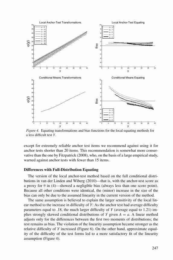
Figure 4. Equating transformations and bias functions for the local equating methods fora less difficult test Y .

except for extremely reliable anchor test items we recommend against using it foranchor tests shorter than 20 items. This recommendation is somewhat more conser-vative than the one by Fitzpatrick (2008), who, on the basis of a large empirical study,warned against anchor tests with fewer than 15 items.

Differences with Full-Distribution Equating

The version of the local anchor-test method based on the full conditional distri-butions in van der Linden and Wiberg (2010)—that is, with the anchor-test score asa proxy for θ in (4)—showed a negligible bias (always less than one score point).Because all other conditions were identical, the (minor) increase in the size of thebias can only be due to the assumed linearity in the current version of the method.

The same assumption is believed to explain the larger sensitivity of the local lin-ear method to the increase in difficulty of Y: As the anchor test had average difficultyparameters equal to .18, the much larger difficulty of Y (average equal to 1.21) im-plies strongly skewed conditional distributions of Y given A = a. A linear methodadjusts only for the differences between the first two moments of distributions; therest remains as bias. The violation of the linearity assumption became stronger as therelative difficulty of Y increased (Figure 6). On the other hand, approximate equal-ity of the difficulty of the test forms led to a more satisfactory fit of the linearityassumption (Figure 4).

247

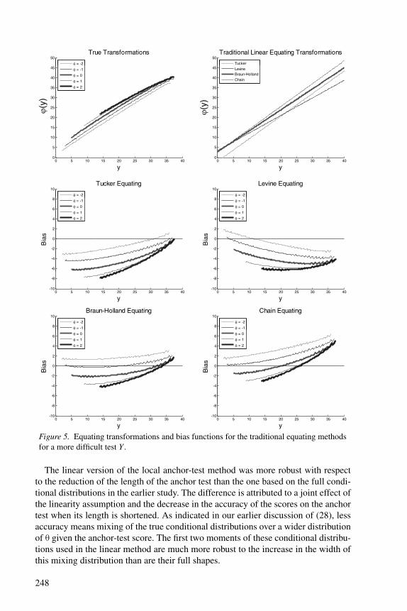
Figure 5. Equating transformations and bias functions for the traditional equating methodsfor a more difficult test Y .

The linear version of the local anchor-test method was more robust with respectto the reduction of the length of the anchor test than the one based on the full condi-tional distributions in the earlier study. The difference is attributed to a joint effect ofthe linearity assumption and the decrease in the accuracy of the scores on the anchortest when its length is shortened. As indicated in our earlier discussion of (28), lessaccuracy means mixing of the true conditional distributions over a wider distributionof θ given the anchor-test score. The first two moments of these conditional distribu-tions used in the linear method are much more robust to the increase in the width ofthis mixing distribution than are their full shapes.

248

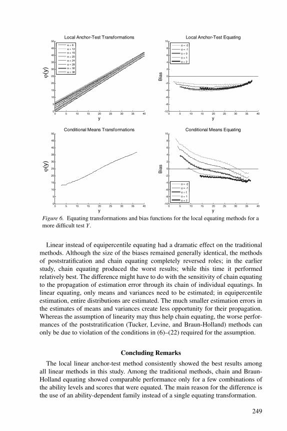
Figure 6. Equating transformations and bias functions for the local equating methods for amore difficult test Y .

Linear instead of equipercentile equating had a dramatic effect on the traditionalmethods. Although the size of the biases remained generally identical, the methodsof poststratification and chain equating completely reversed roles; in the earlierstudy, chain equating produced the worst results; while this time it performedrelatively best. The difference might have to do with the sensitivity of chain equatingto the propagation of estimation error through its chain of individual equatings. Inlinear equating, only means and variances need to be estimated; in equipercentileestimation, entire distributions are estimated. The much smaller estimation errors inthe estimates of means and variances create less opportunity for their propagation.Whereas the assumption of linearity may thus help chain equating, the worse perfor-mances of the poststratification (Tucker, Levine, and Braun-Holland) methods canonly be due to violation of the conditions in (6)–(22) required for the assumption.

Concluding Remarks

The local linear anchor-test method consistently showed the best results amongall linear methods in this study. Among the traditional methods, chain and Braun-Holland equating showed comparable performance only for a few combinations ofthe ability levels and scores that were equated. The main reason for the difference isthe use of an ability-dependent family instead of a single equating transformation.

249

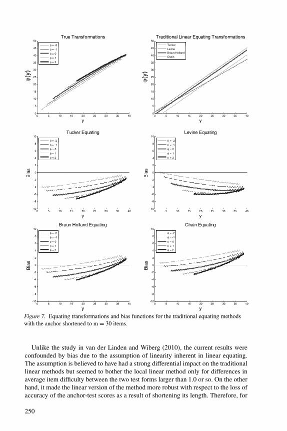
Figure 7. Equating transformations and bias functions for the traditional equating methodswith the anchor shortened to m = 30 items.

Unlike the study in van der Linden and Wiberg (2010), the current results wereconfounded by bias due to the assumption of linearity inherent in linear equating.The assumption is believed to have had a strong differential impact on the traditionallinear methods but seemed to bother the local linear method only for differences inaverage item difficulty between the two test forms larger than 1.0 or so. On the otherhand, it made the linear version of the method more robust with respect to the loss ofaccuracy of the anchor-test scores as a result of shortening its length. Therefore, for

250

Figure 8. Equating transformations and bias functions for the traditional equating methodswith the anchor shortened to m = 20 items.

longer anchors the local method for the full conditional distributions should be pre-ferred over the linear method, but for shorter anchors the linear method is expectedto perform better (at the price of a slightly increased bias). In fact, these preferencesare entirely in line with the bias-accuracy trade-off discussed in the introduction tothis paper to motivate linear equating.

Reversely, the full local method appeared to be more robust to extreme differencesin difficulty between the test forms, but the linear method was sensitive to them

251

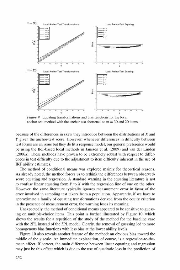
Figure 9. Equating transformations and bias functions for the localanchor-test method with the anchor test shortened to m = 30 and 20 items.

because of the differences in skew they introduce between the distributions of X andY given the anchor-test score. However, whenever differences in difficulty betweentest forms are an issue but they do fit a response model, our general preference wouldbe using the IRT-based local methods in Janssen et al. (2009) and van der Linden(2006a). These methods have proven to be extremely robust with respect to differ-ences in test difficulty due to the adjustment to item difficulty inherent in the use ofIRT ability estimates.

The method of conditional means was explored mainly for theoretical reasons.As already noted, the method forces us to rethink the differences between observed-score equating and regression. A standard warning in the equating literature is notto confuse linear equating from Y to X with the regression line of one on the other.However, the same literature typically ignores measurement error in favor of theerror involved in sampling test takers from a population. Apparently, if we have toapproximate a family of equating transformations derived from the equity criterionin the presence of measurement error, the warning loses its meaning.

Unexpectedly, the method of conditional means appeared to be sensitive to guess-ing on multiple-choice items. This point is further illustrated by Figure 10, whichshows the results for a repetition of the study of the method for the baseline casewith the 2PL instead of the 3PL model. Clearly, the removal of guessing led to morehomogenous bias functions with less bias at the lower ability levels.

Figure 10 also reveals another feature of the method: an obvious bias toward themiddle of the y scale. An immediate explanation, of course, is a regression-to-the-mean effect. If correct, the main difference between linear equating and regressionmay just be this effect which is due to the use of quadratic loss in the prediction of

252

Figure 10. Equating transformations and bias functions for the method of conditionalmeans for the 2PL model (baseline case).

one score from the other in the latter. In principle, it might be simple to correct for it;the bias functions in Figure 10 appear to be amazingly straight, and their slope mayrelate directly to the reliability of X. But this topic, as well as several other aspects ofthe method of conditional means, requires further study before we can recommendusing (a modification of) it in practice.

References

Braun, H. I., & Holland, P. W. (1982). Observed-score test equating: A mathematical analysisof some ETS equating procedures. In P. W Holland & D. B. Rubin (Eds.), Test equating(pp. 9–49). New York, NY: Academic Press.

Cook, L. L., & Petersen, N. S. (1987). Problems related to the use of conventional and item re-sponse theory equating methods in less than optimal circumstances. Applied PsychologicalMeasurement, 25, 225–244.

Dorans, N. J. (1990). Equating methods and sampling designs. Applied Measurement in Edu-cation, 3, 3–17.

Dorans, N. J., & Holland, P. W. (2000). Population invariance and the equatability of tests:Basic theory and the linear case. Journal of Educational Measurement, 37, 281–306.

Fitzpatrick, A. R. (2008). The impact of anchor-test configuration on student proficiency rates.Educational Measurement: Issues and Practice, 27(4), 34–40.

Janssen, R., Magis, D., San Martin, E., & Del Pino, G. (2009, April). Local equating in theNEAT design. Paper presented at the meeting of the National Council on Measurement inEducation, San Diego, CA.

Kolen, M. J., & Brennan, R. L. (2004). Test equating, scaling, and linking: Methods andpractices (2nd ed.). New York, NY: Springer.

Liou, M., Cheng, P. E., & Li, M.-Y. (2001). Estimating comparable scores using surrogatevariables. Applied Psychological Measurement, 25, 197–207.

Livingston, S. A., Dorans, N. J., & Wright, N. K. (1990). What combination of sampling andequating methods work best? Applied Measurement in Education, 3, 73–95.

Lord, F. M. (1980). Applications of item response theory to practical testing problems.Hillsdale, NJ: Erlbaum.

Lord, F. M., & Wingersky, M. S. (1984). Comparison of IRT true-score and equipercentileobserved-score “equatings”. Applied Psychological Measurement, 8, 452–461.

253

Wiberg and van der Linden

Petersen, N. S., Marco, G. L., & Stewart, E. E. (1982). A test of the adequacy of linear scoreequating models. In P. W. Holland & D. B. Rubin (Eds.), Test equating (pp. 71–135). NewYork, NY: Academic Press.

van der Linden, W. J. (2000). A test-theoretic approach to observed score equating. Psychome-trika, 65, 437–456.

van der Linden, W. J. (2006a). Equating error in observed-score equating. Applied Psycholog-ical Measurement, 30, 355–378.

van der Linden, W. J. (2006b). Equating scores from adaptive to linear tests. Applied Psycho-logical Measurement, 30, 493–508.

van der Linden, W. J. (2011). Local observed-score equating. In A. A. von Davier (Ed.), Sta-tistical models for equating, scaling, and linking (pp. 201–223). New York, NY: Springer.

van der Linden, W.J., & Wiberg, M. (2010). Local observed-score equating with anchor-testdesigns. Applied Psychological Measurement, 34, 620–640.

von Davier, A. A., Holland, P. W., & Thayer, D. T. (2004a). The kernel method of test equating.New York, NY: Springer.

von Davier, A. A., Holland, P. W., & Thayer, D. T. (2004b). The chain and post-stratificationmethods for observed-score equating: Their relationship to population invariance. Journalof Educational Measurement, 41, 15–32.

von Davier, A. A., & Kong, N. (2005). A unified approach to linear equating for the nonequiv-alent groups design. Journal of Educational and Behavioral Statistics, 30, 313–342.

Wilk, M. B., & Gnanadesikan, R. (1968). Probability plotting methods for the analysis of data.Biometrika, 55, 1–17.

Wright, N. K., & Dorans, N. J. (1993). Using the selection variable for matching and equating(Research Report No. 94-04). Princeton, NJ: Educational Testing Service.

Authors

MARIE WIBERG is an Associate Professor, Department of Statistics, Umea University,SE-90187 Umea, Sweden; marie.wiberg@stat.umu.se. Her primary research interestsinclude psychometrics, test equating, applied statistics, and international large-scaleassessments.

WIM J. VAN DER LINDEN is Chief Research Scientist, CTB/McGraw-Hill, 20 Ryan RanchRoad. Monterey, CA 93940; wim vanderlinden@ctb.com. His primary research interestsinclude test theory, applied statistics, and research methods.

254