Local False Discovery RatesBradley Efron

Abstract

Modern scientific technology is providing a new class of large-scale simultaneousinference problems, with hundreds or thousands of hypothesis tests to consider at thesame time. Microarrays epitomize this type of technology but similar problems arisein proteomics, time of flight spectroscopy, flow cytometry, FMRI imaging, and massivesocial science surveys. This paper uses local false discovery rate methods to carryout size and power calculations on large-scale data sets. An empirical Bayes approachallows the fdr analysis to proceed from a minimum of frequentist or Bayesian modelingassumptions. Microarray and simulated data sets are used to illustrate a convenientestimation methodology whose accuracy can be calculated in closed form. A crucialpart of the methodology is an fdr assessment of “thinned counts”, what the histogramof test statistics would look like for just the non-null cases.

1. Introduction

Large-scale simultaneous hypothesis testing problems, with hundreds or thousands ofcases considered together, have become a fact of current-day statistical practice. Microarraymethodology spearheaded the production of large-scale data sets, but other “high through-put” technologies are emerging, including time of flight spectroscopy, proteomic devices, flowcytometry, and functional Magnetic Resonance Imaging.

Benjamini and Hochberg’s seminal (1995) paper introduced False Discovery Rates (Fdr),a particularly useful new approach to simultaneous testing. Fdr theory relies on p-values,that is on null hypothesis tail areas, and as such operates as an extension of traditionalfrequentist hypothesis testing to simultaneous inference, whether involving just a few casesor several thousand. Large-scale situations, however, permit another approach: empiricalBayes methods can bring Bayesian ideas to bear without the need for strong Bayesian orfrequentist assumptions. Local false discovery rates (fdr), the subject of this paper, useempirical Bayes techniques to provide both size and power calculations for large-scale studies.

The data for one such study is summarized in Figure 1. Eight microarrays, four from cellsof HIV infected subjects and four from uninfected subjects, have each measured expressionlevels for the same N = 7680 genes. Each gene yields a two-sample t-statistic ti comparingthe infected versus the uninfected subjects, which is then transformed to a z-value,

zi = Φ−1(F6(ti)), (1.1)

where F6 is the cumulative distribution function (cdf) of a standard t variable with 6 de-grees of freedom, and Φ is the standard normal cdf. Theoretically zi should have a N(0, 1)distribution if gene i produces identically distributed normal expressions for infected anduninfected cells.

The histogram of z-values shown in Figure 1 looks promising: the normal-shaped centralpeak presumably charts the large majority of “null” genes, those behaving similarly forinfected and uninfected cells, while the long tails reveal some interesting “non-null” genes,the kind the study, was intended to detect; fdr methodology, described in Section 5, hasbeen used to provide thinned counts, an estimate of what a histogram of only the non-nullz-values would look like.

Figure 2 shows the estimated local false discovery rate curve fdr(z) based on empiricalBayes methodology discussed in Sections 3 and 4; fdr(z), the conditional probability of a casebeing null given z, declines from one near z = 0 to zero at the extremes. There are 186 geneshaving fdr(z) ≤ 0.2, a reasonable cutoff point discussed in Section 2, and we might reportthese 186 to the investigators as interesting candidates for further study. Other methods,such as Benjamini and Hochberg’s Fdr procedure with cutoff q = 0.1, yield similar results.

Figure 2 also displays the thinned counts from Figure 1, estimating the histogram ofnon-null genes. Strikingly, a majority of the non-null cases lie well within the 0.2 fdr cutofflimits. However if we try to report more of the non-null cases then false discovery rates

1

Figure 1: Histogram of 7680 z-values from an HIV microarray experiment. Short verticalbars are estimated “thinned counts” of non-null genes, as explained in Section 5. (Extremevalues have been truncated, giving small bars at each end.) Data from van’t Wout et al.(2003), discussed in Gottardo et al. (2004).

can grow unacceptably large, say to fdr(z) = 0.5, where the investigator would have a 50%chance of pursuing false leads.

In other words the HIV study is underpowered. Section 5 describes power diagnosticsfor large-scale testing situations, based on fdr calculations of the type shown Figure 2.

Section 6 discusses the non-null distribution of z-values such as (1.1). It suggests thatthe underlying densities for histograms like Figure 1’s should be smooth normal mixtures,smoothness being an important assumption of our fdr methodology.

Ideally, a big data set like that of the HIV study should require very little paramet-ric modeling, the data itself providing the framework for its own analysis. This ideal isapproached by the fdr calculations for Figures 1 and 2, which depend on a simple model,presented in Section 2, requiring few assumptions. Section 7 examines this model in termsof a more structured formulation, clarifying its limitations in regard to bias and the choiceof null hypothesis.

Focusing on z-values, rather than working within the full 7680 × 8 data matrix forthe HIV study, greatly reduces the need for modeling assumptions. There will certainlybe situations where working inside the matrix, as in Newton et al. (2004), Gottardo etal. (2004), and Kerr, Martin, and Churchill (2000), yields more information. Using suchmethods requires more careful attention to the details of the individual data set than ourrelatively crude z-value approach. A key assumption not made here is independence acrossthe columns of the data matrix (e.g. independence across microarrays) which underlies theuse of permutation or bootstrap methods for null hypothesis testing distributions. In factthere turns out to be curious dependences across the HIV matrix, as mentioned in Section3.2, similar to the correlation effects in the microarray example of Efron (2004); column-wiseindependence seems to be a dangerous assumption for microarray studies.

A substantial microarray statistics literature has developed in the past few years, much

2

Figure 2: Heavy curve is fdr(z), local false discovery rate as estimated by locfdr algorithmdescribed in Section 3; fdr(z) = 0.2 at z = −2.34 and 2.17. Vertical bars are thinned countsfrom Figure 1, now multiplied by 0.01 and plotted negatively.

of it focused on the control of frequentist Type I errors, see for example Dudoit, van derLaan and Pollard (2004), and the review article by Dudoit, Shaffer, and Boldruck (2003).Bayes and empirical Bayes methods have also been advocated, as in Kendziorski et al. (2003),Johnstone and Silverman (2004), and Newton et al. (2004), while Benjamini and Hochberg’sFdr theory is increasingly influential, see Storey et al. (2004), and Genovese and Wasserman(2004). Local fdr methods, which this article argues can play a useful role, were introducedin Efron et al. (2001); several references are listed at the end of Section 3.1.

2. False Discovery Rates

Local false discovery rates, Efron et al. (2001), Efron and Tibshirani (2002), are avariant of Benjamini and Hochberg’s (1995) “tail area” false discovery rates. This sectionrelates the two ideas, reviews a few basic properties, and presents some general guidelines forinterpreting fdr’s. The development here is theoretical, with practical estimation proceduresdeferred to Section 3.

Suppose we have N null hypotheses to consider simultaneously, each with its own teststatistic,

Null hypothesis : H1,H2,...,Hi,...,HN

Test statistic : z1, z2,..., zi,..., zN

(2.1)

N must be large for local fdr calculations, at least in the hundreds, but the zi need not beindependent. A simple Bayesian model, Lee et al. (2000), Newton et al. (2001), Efron et al.(2001), underlies the theory: we assume that the N cases are divided into two classes, nullor non-null, occurring with prior probabilities p0 or p1 = 1− p0, and with the density of test

3

statistic z depending upon its class,

p0 = Pr{null} f0(z) density if null

p1 = Pr{non-null} f1(z) density if non-null.(2.2)

In context (1.1) it is natural to take f0(z) to be the standard N(0, 1) density – but see Section3.2 – and f1(z) some longer-tailed density, perhaps representing a mixture of alternativepossibilities; the empirical estimation theory of Section 3 does not require specification off1(z). Practical applications of large-scale testing usually assume a large p0 value, say

p0 ≥ 0.9, (2.3)

the goal being to identify a relatively small set of interesting non-null cases.

Define the null subdensityf+

0 (z) = p0f0(z) (2.4)

and the mixture densityf(z) = p0f0(z) + p1f1(z). (2.5)

The Bayes posterior probability that a case is null given z, by definition the local falsediscovery rate, is

fdr(z) ≡ Pr{null|z} = p0f0(z)/f(z)

= f+0 (z)/f(z).

(2.6)

The Benjamini-Hochberg false discovery rate theory relies on tail areas rather thandensities. Letting F0(z) and F1(z) be the cdf’s corresponding to f0(z) and f1(z) in (2.2),define F+

0 (z) = p0F0(z) and F (z) = p0F0(z) + p1F1(z). Then the posterior probability of acase being null given that its z-value “Z” is less than some value z is

Fdr(z) ≡ Pr{null|Z ≤ z} = F+0 (z)/F (z). (2.7)

(It is notationally convenient to consider events Z ≤ z but we could just as well consider tailareas to the right, two-tailed events, etc.) Figure 3 illustrates the geometrical relationshipbetween Fdr and fdr.

Benjamini and Hochberg’s FDR control rule depends on an estimated version of (2.6)where F is replaced by the empirical cdf. Storey (2002) and Efron and Tibshirani (2002)discuss the connection of the frequentist FDR procedure with Bayesian form (2.7). Fdr(z)corresponds to Storey’s “q-value”, the value of the tail area false discovery rate attained ata given observed value Z = z.

Fdr and fdr are analytically related by

Fdr(z) =

∫ z

−∞fdr(Z)f(Z)dZ/

∫ z

−∞f(Z)dZ

= Ef{fdr(Z)|Z ≤ z},(2.8)

4

Figure 3: Geometrical relationship of Fdr to fdr; heavy curve plots F+0 (z) versus F (z);

fdr(z) is slope of tangent, Fdr(z) slope of secant.

“Ef” indicating expectations with respect to f(z), Efron and Tibshirani (2002). That is,Fdr(z) is the average of fdr(Z) for Z ≤ z; Fdr(z) will be less than fdr(z) in the usual situationwhere fdr(z) decreases as |z| gets large. For example fdr(−2.34) = 0.20 in Figure 2 whileFdr(−2.34) = 0.12. If the cdf’s F0(z) and F1(z) are Lehmann alternatives

F1(z) = F0(z)α, [α < 1], (2.9)

it is straightforward to show that

log

{fdr(z)

1 − fdr(z)

}= log

{Fdr(z)

1 − Fdr(z)

}+ log

(1

α

), (2.10)

givingfdr(z) = Fdr(z)/α (2.11)

for small values of Fdr. The HIV data of Figure 1 has α roughly 1/2 in the left tail and 1/3in the right.

The local nature of fdr(z) is an advantage in interpreting results for individual cases.For example, a gene with z = 2.0 in the HIV study has an estimated fdr of 0.30 while thecorresponding (right-sided) tail-area Fdr, the q-value, is 0.12. Quoting just this last numbergives an overoptimistic impression of the gene’s significance. In practice the methods canbe combined, using the Benjamini-Hochberg algorithm to identify non-null cases, say withq = 0.10, but also providing individual fdr values for those cases.

The literature has not reached consensus on a standard choice of q for Benjamini-Hochberg testing, the equivalent of .05 for single tests, but Bayesian calculations offer someinsight. The cutoff threshold fdr ≤ 0.20 used in Figure 2 yields posterior odds ratio

Pr{non-null|z}/Pr{null|z} = (1 − fdr(z))/fdr(z)

= p1f1(z)/p0f0(z) ≥ 0.8/0.2 = 4.(2.12)

5

If we assume prior odds ratio p1/p0 ≤ 0.1/0.9 as in (2.3), then (2.12) corresponds to Bayesfactor

f1(z)/f0(z) ≥ 36 (2.13)

in favor of non-null.

This threshold requires a much stronger level of evidence against the null hypothesisthen in standard one-at-a-time testing. For instance suppose we observe x ∼ N(µ, 1) andwish to test H0 : µ = 0 vs µ = 2.80, a familiar scenario for power calculations sincerejecting H0 for x ≥ 1.96 yields two-sided size 0.05 and power 0.80. Here the criticalBayes factor is only f2.80(1.96)/f0(1.96) = 4.80. (A value closer to 3 is suggested by themore careful considerations in Efron and Gous (2001).) We might justify (2.13) as beingconservative in guarding against multiple testing fallacies. More pragmatically, increasing thefdr threshold much above 0.20 can deliver unacceptably high proportions of false discoveriesto the investigators. The 0.20 threshold, used in the remainder of the paper, corresponds toq-values between 0.05 and 0.15 for reasonable choices of α in (2.11); such q-value thresholdscan be interpreted as reflecting a conservative Bayes factor for Fdr interpretation.

Any choice of threshold is liable to leave investigators complaining that the statisticians’list of non-null cases omits some of their a priori favorites. Conveying the full list of valuesfdr(zi), not just those for cases judged non-null, allows investigators to employ their ownprior opinions on interpreting significance. This is particularly important for low-poweredsituations like the HIV study, where luck plays a big role in any one case’s results, but it isthe counsel of perfection, and most investigators will require some sort of reduced list.

False discovery rates, both fdr and Fdr, depend on only the marginal distribution ofthe z values, f(z) or F (z). This has both good and bad consequences: On the good side,independence is not required of the zi’s in (2.1), since all that is needed is a reasonableestimate of their marginal distribution. Less happily, results like (2.6) or (2.7) are really“one-at-a-time” Bayes inferences, that may be quite different than the (usually unknowable)posterior probability of Hi given the entire N -vector z.

3. Estimating fdr

The heavy curve in Figure 2 is an estimate of the local false discovery rate fdr(z) forthe HIV study. This section concerns the estimate’s empirical Bayes methodology, includingthe question of choosing an appropriate null hypothesis. Accuracy of the estimation pro-cedure is taken up in Section 4. (This methodology is available through algorithm locfdr,Comprehensive R Archive Network, http://cran.r-project.org.) Estimating the numeratorand denominator of fdr(z) = f+

0 (z)/f(z) will be discussed separately.

3.1 Estimating the Mixture Density f(z)

Nonparametric density estimation has a reputation for difficulty, well-deserved in generalsituations. However there are good theoretical reasons for believing that z-value distributionsare quite smooth, see Section 6. Our tactic here is to estimate the mixture density f(z),the denominator of fdr(z) in (2.6), with smooth but flexible parametric models. Section 4discusses the accuracy of this approach.

Lindsey’s method, as discussed in Section 2 of Efron and Tibshirani (1996), permits effi-cient and flexible parametric density estimation using standard Poisson regression software.

6

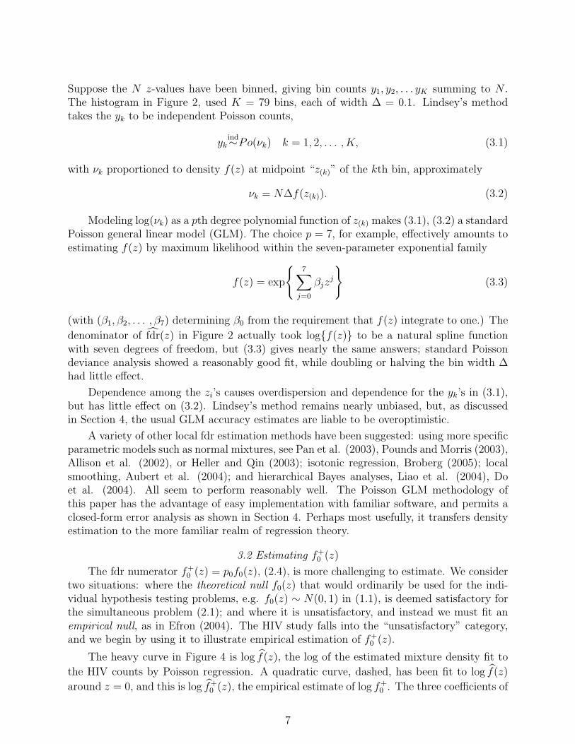
Suppose the N z-values have been binned, giving bin counts y1, y2, . . . yK summing to N .The histogram in Figure 2, used K = 79 bins, each of width ∆ = 0.1. Lindsey’s methodtakes the yk to be independent Poisson counts,

ykind∼Po(νk) k = 1, 2, . . . , K, (3.1)

with νk proportioned to density f(z) at midpoint “z(k)” of the kth bin, approximately

νk = N∆f(z(k)). (3.2)

Modeling log(νk) as a pth degree polynomial function of z(k) makes (3.1), (3.2) a standardPoisson general linear model (GLM). The choice p = 7, for example, effectively amounts toestimating f(z) by maximum likelihood within the seven-parameter exponential family

f(z) = exp

{7∑

j=0

βjzj

}(3.3)

(with (β1, β2, . . . , β7) determining β0 from the requirement that f(z) integrate to one.) The

denominator of fdr(z) in Figure 2 actually took log{f(z)} to be a natural spline functionwith seven degrees of freedom, but (3.3) gives nearly the same answers; standard Poissondeviance analysis showed a reasonably good fit, while doubling or halving the bin width ∆had little effect.

Dependence among the zi’s causes overdispersion and dependence for the yk’s in (3.1),but has little effect on (3.2). Lindsey’s method remains nearly unbiased, but, as discussedin Section 4, the usual GLM accuracy estimates are liable to be overoptimistic.

A variety of other local fdr estimation methods have been suggested: using more specificparametric models such as normal mixtures, see Pan et al. (2003), Pounds and Morris (2003),Allison et al. (2002), or Heller and Qin (2003); isotonic regression, Broberg (2005); localsmoothing, Aubert et al. (2004); and hierarchical Bayes analyses, Liao et al. (2004), Doet al. (2004). All seem to perform reasonably well. The Poisson GLM methodology ofthis paper has the advantage of easy implementation with familiar software, and permits aclosed-form error analysis as shown in Section 4. Perhaps most usefully, it transfers densityestimation to the more familiar realm of regression theory.

3.2 Estimating f+0 (z)

The fdr numerator f+0 (z) = p0f0(z), (2.4), is more challenging to estimate. We consider

two situations: where the theoretical null f0(z) that would ordinarily be used for the indi-vidual hypothesis testing problems, e.g. f0(z) ∼ N(0, 1) in (1.1), is deemed satisfactory forthe simultaneous problem (2.1); and where it is unsatisfactory, and instead we must fit anempirical null, as in Efron (2004). The HIV study falls into the “unsatisfactory” category,and we begin by using it to illustrate empirical estimation of f+

0 (z).

The heavy curve in Figure 4 is log f(z), the log of the estimated mixture density fit to

the HIV counts by Poisson regression. A quadratic curve, dashed, has been fit to log f(z)

around z = 0, and this is log f+0 (z), the empirical estimate of log f+

0 . The three coefficients of

7

the fitted quadratic determine f+0 (z) as a scaled normal density, in this case with p0 = 0.917

and f0 ∼ N(−0.10, 0.742),

f0(z) = .917 · ϕ−.10,.74(z)

[ϕδ,σ(z) = exp

{− 1

2

(z − δ

σ

)2}/√2πσ2

]. (3.4)

The default option in locfdr fits a quadratic to log f(z) by ordinary least squares appliedover the central one-third range of the z-values.

Figure 4: Empirical estimation of the fdr numerator f+0 (z) = p0f0(z), HIV study. Heavy

curve is log of Poisson regression estimate f(z) for mixture density; dashed curve is log f+0 (z),

best-fitting quadratic to log f(z) near z = 0; estimates p0 = 0.917, f0 ∼ N(−0.10, 0.742).

Dotted curve is log f+0 for theoretical null.

The logic here is quite simple: we make the “zero assumption” that the central peakof Figure 1’s histogram consists mainly of null cases, and choose p0, δ and σ in (3.4) toquadratically approximate the histogram counts near z = 0. This same argument can beapplied with the theoretical null, giving the dotted curve in Figure 4. Now f0(z) is assumedto be ϕ0,1(z), the standard normal, so only p0 in f+

0 = p0f0 remains to be estimated fromthe central histogram counts.

The two-class model (2.2) is unidentifiable without restrictions on the form of f0 andf1. Some version of the zero assumption is necessary in the absence of strong parametricassumptions, see for example Section 3 of Storey (2002). (Most of the FDR literature workswith p-values rather than z-values, pi = F6(ti) in (1.1), in which case the “zero region” occursnear p = 1.) The zero assumption is more believable when p0, the proportion of null cases, is

8

near 1. Efron (2004), Section 5, shows that if p0 exceeds 0.90, the fitting method of Figure 4will have negligible bias: although the 10% or less of non-null cases might in fact contributesome counts near z = 0, these cannot substantially affect the estimates of δ and σ in (3.4).The estimate of p0 is affected, being upwardly biased as seen in Section 4 and discussed inSection 7.

The theoretical null hypothesis f0 ∼ N(0, 1) is untenable for the HIV data. If it werevalid then f(z) should be at least as wide as f0 near z = 0, assuming that non-null z’s aremore dispersed than nulls. Instead f is substantially narrower, forcing f+

0 = p0f0 to takethe impossible value p0 = 1.15 in order to match the histogram heights near z = 0.

The examples in Efron (2004) go the other way: in both of them the empirical null issubstantially wider than N(0, 1). Various causes of overdispersion are suggested, includinghidden correlations and unobserved covariates. The underdispersion here is harder to explain,but can be traced to a correlation of expression levels across microarrays: levels on the odd-numbered arrays were positively correlated, as were levels among the even-numbered arrays,the effect cutting across the Treatment-Control classification, a pattern that swelled thedenominators of the t-statistics (1.1).

Misspecification of the null hypothesis, which becomes visible in large-scale testing sit-uations, undermines all forms of simultaneous inference, fdr, Fdr, Bonferroni, Family-WiseError Rate, or the sophisticated resampling based algorithms of Westfall and Young (1993).Using an empirical null avoids the problem, but at a substantial cost in estimation efficiencyas shown in Section 4. Other methods are sometimes available for empirical null estimation,involving “housekeeper genes” (cases known a priori to be null) and designed replications,as in Lee et al. (2000).

More ambitiously, one may try to model the full error structure of the original data set,a 7680 × 8 matrix in the HIV study, using frequentist or Bayesian modeling as in Kerr andChurchill (2001), or Newton et al. (2004). When feasible this is the ideal approach but itcan be an heroic undertaking in the complicated venue of microarray analysis. The approachhere, relying only on the observed distribution of the z-values, trades some loss of efficiencyfor fewer assumptions and simple application.

Permutation and bootstrap null density estimates play a major role in the microarrayliterature, as in Tusher et al. (2001) and Pollard and van der Laan (2003). These shouldbe considered as improved versions of the theoretical null rather than empirical nulls. Thepermutation null for the HIV data, permuting the eight microarrays, is about N(0, .992).

Figure 4’s quadratic construction assumes that f0 is normal, but uses the data to estimateits mean and variance instead of accepting the theoretical choice N(0, 1). Under somecircumstances we might wish to go further, perhaps adding a cubic term to log f0; locfdrincludes such an option, described in Section 7.

The basic false discovery rate idea is appealingly simple: 19 of the HIV z-values fellinto bin [2.0, 2.1] in Figure 1, the smoothed estimate from f being 19.95; this compares with

expected number 4.70 under f+0 , yielding estimated local false discovery rate 4.70/19.95 =

0.24. If we report this bin as containing interesting cases, then about one-fourth of themwill turn out to be false discoveries. The question of the accuracy of this estimate is takenup next.

9

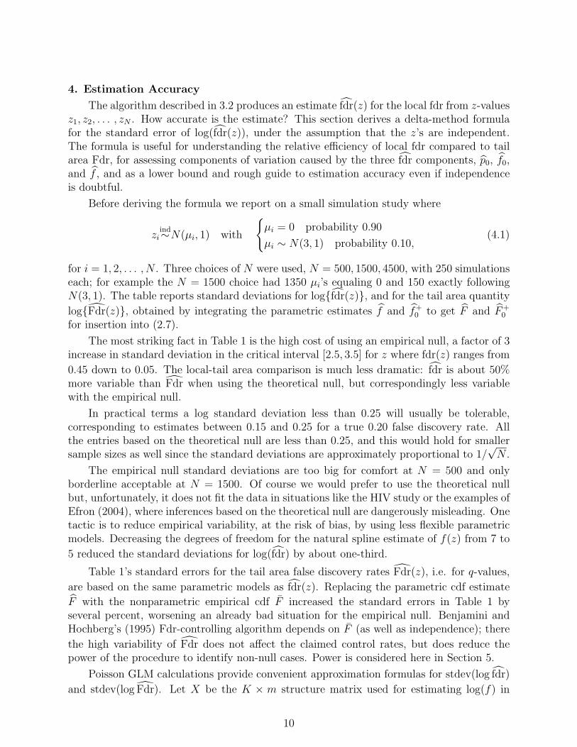
4. Estimation Accuracy

The algorithm described in 3.2 produces an estimate fdr(z) for the local fdr from z-valuesz1, z2, . . . , zN . How accurate is the estimate? This section derives a delta-method formulafor the standard error of log(fdr(z)), under the assumption that the z’s are independent.The formula is useful for understanding the relative efficiency of local fdr compared to tailarea Fdr, for assessing components of variation caused by the three fdr components, p0, f0,and f , and as a lower bound and rough guide to estimation accuracy even if independenceis doubtful.

Before deriving the formula we report on a small simulation study where

ziind∼N(µi, 1) with

{µi = 0 probability 0.90

µi ∼ N(3, 1) probability 0.10,(4.1)

for i = 1, 2, . . . , N . Three choices of N were used, N = 500, 1500, 4500, with 250 simulationseach; for example the N = 1500 choice had 1350 µi’s equaling 0 and 150 exactly followingN(3, 1). The table reports standard deviations for log{fdr(z)}, and for the tail area quantity

log{Fdr(z)}, obtained by integrating the parametric estimates f and f+0 to get F and F+

0

for insertion into (2.7).

The most striking fact in Table 1 is the high cost of using an empirical null, a factor of 3increase in standard deviation in the critical interval [2.5, 3.5] for z where fdr(z) ranges from

0.45 down to 0.05. The local-tail area comparison is much less dramatic: fdr is about 50%more variable than Fdr when using the theoretical null, but correspondingly less variablewith the empirical null.

In practical terms a log standard deviation less than 0.25 will usually be tolerable,corresponding to estimates between 0.15 and 0.25 for a true 0.20 false discovery rate. Allthe entries based on the theoretical null are less than 0.25, and this would hold for smallersample sizes as well since the standard deviations are approximately proportional to 1/

√N .

The empirical null standard deviations are too big for comfort at N = 500 and onlyborderline acceptable at N = 1500. Of course we would prefer to use the theoretical nullbut, unfortunately, it does not fit the data in situations like the HIV study or the examples ofEfron (2004), where inferences based on the theoretical null are dangerously misleading. Onetactic is to reduce empirical variability, at the risk of bias, by using less flexible parametricmodels. Decreasing the degrees of freedom for the natural spline estimate of f(z) from 7 to

5 reduced the standard deviations for log(fdr) by about one-third.

Table 1’s standard errors for the tail area false discovery rates Fdr(z), i.e. for q-values,

are based on the same parametric models as fdr(z). Replacing the parametric cdf estimate

F with the nonparametric empirical cdf F increased the standard errors in Table 1 byseveral percent, worsening an already bad situation for the empirical null. Benjamini andHochberg’s (1995) Fdr-controlling algorithm depends on F (as well as independence); there

the high variability of Fdr does not affect the claimed control rates, but does reduce thepower of the procedure to identify non-null cases. Power is considered here in Section 5.

Poisson GLM calculations provide convenient approximation formulas for stdev(log fdr)

and stdev(log Fdr). Let X be the K × m structure matrix used for estimating log(f) in

10

Section 3.1; X has m = 8, kth row (1, z(k), z2(k), . . . , z7

(k)) in model (3.3). Also let X0 be the

K ×m0 matrix used to describe log(f+0 ) in Section 3.2: X0 has kth row (1, z(k), z

2(k)) for the

empirical null, m0 = 3, while X0 is the K × 1 matrix (1, 1, . . . , 1)′ for the theoretical null.

Locfdr fits log f+0 (z) to log f(z) over a central subset of K0 bins, with index set say “i0”,

defining submatrices with rows in i0,

X = X[i0, ] and X0 = X0[i0, ] (4.2)

of dimensions K0 × m and K0 × m0. Also define inner product matrices

G = X ′ diag (ν)X and G0 = X ′0X0, (4.3)

where diag (ν) is the K × K diagonal matrix having diagonal elements νk = N∆f(z(k)) asin (3.2).

Finally, let � indicate the K-vector with elements �k = log f(z(k)), likewise �+0 for vector

(log f+0 (z(k))) and �fdrk for log fdr(z(k)).

Lemma 1 The K × K derivative matrix of log fdr with respect to the bin counts is(d �fdrk

dy�

)= AG−1X ′, (4.4)

whereA = X0G

−10 X ′

0X − X. (4.5)

Proof A small change dy in the count vector (considered as continuous) produces change

d� in �,d� = XG−1X ′dy. (4.6)

Similarly if �+0 = X0γ, γ a m0-vector, is fit by least squares to � = �[i0], we have

dγ = G−10 X ′

0d� and d�+0 = X0G

−10 X ′

0d�. (4.7)

Both (4.6) and (4.7) are standard regression results. Then (4.6) gives d� = d�[i0] =

XG−1X ′dy, yieldingd�+

0 = X0G−10 X ′

0XG−1X ′dy (4.8)

from (4.7). Finally,

d(�fdr) = d(�+0 − �) = (X0G

−10 X ′

0X − X)G−1X ′dy, (4.9)

verifying (4.4). �The delta-method estimate of covariance for the K-vector �fdr is derived from the lemma

ascov(�fdr) = (AG−1X ′)cov(y)(AG−1X ′)′

= (AG−1X ′)diag(ν)(AG−1X ′)′,(4.10)

11

under Poisson assumptions (3.1), (3.2). Since G = X ′ diag (ν)X this reduces to a relativelysimple formula:

Theorem The delta-method estimate of covariance for the vector of log fdr(z(k)) values is

cov(�fdr) = AG−1A (4.11)

with A as in (4.5).

The entries “form” in Table 1 are square roots of diagonal elements of cov in (4.11), av-eraged over the 250 simulations. They produced reasonable estimates of the actual standarddeviations of log (fdr), especially for the empirical null.

A formula similar to (4.11) exists for the tail area false discovery rates �Fdrk = log Fdr(z(k)),

cov(�Fdr) = BG−1B′, (4.12)

B = S0X0G−10 X ′

0X − SX, (4.13)

where, for the case of left-tail Fdr’s, S0 and S are lower triangular matrices,

Sk� =f�

Fk

and S0k� =f0�

F0k

for � ≤ k. (4.14)

Comparisons of (4.11) with (4.12) in various situations confirm the general story of Table

1: fdr is somewhat more variable than Fdr when using theoretical nulls, the opposite beingtrue for empirical nulls; however both methods are much more variable in the empirical case,this effect dwarfing their comparative differences. (Empirical nulls fare better in the powercalculations of Section 5.)

Table 2 displays means and standard deviations in simulation (4.1) for the three esti-mated parameters of the empirical null, p0, δ, and σ, (3.4). Notice that p0 is biased upward

from the simulation value p0 = 0.90. This makes little difference to fdr(z) = p0f0(z)/f(z),only increasing it by factor .0924/0.90 = 1.03. (The power calculations of Section 5 are moresensitive to bias.) Upward bias arises from the zero assumption: the µ ∼ N(3, 1) compo-nent of (4.1) gives z ∼ N(3, 2), resulting in a small proportion of non-null z-values near 0.However the “bias” here reflects, at least partly, an ambiguity in what p0 actually means, asdiscussed in Section 7.

The variability in the estimated mean and standard deviation of the empirical null, δand σ, has an order of magnitude bigger effect than p0 on fdr and Fdr. The theoretical null“knows” that (δ, σ) = (0, 1), eliminating this variability and accounting for its much smallerstandard deviations.

For fixed z, log fdr(z) is a sum of three terms,

log fdr(z) = log p0 + log f0(z) − log f(z), (4.15)

allowing an exact apportionment of variability of log fdr(z) to the three components. For theempirical null with N = 1500 and z = 2.9 (the point where fdr(z) = 0.20 in model (4.1)) the

12

THEORETICAL NULL EMPIRICAL NULL

z ave(fdr) local (form) tail local (form) tail

N = 5001.5 .95 .08 (.09) .09 .06 (.07) .172.0 .77 .15 (.15) .08 .17 (.17) .272.5 .45 .17 (.18) .08 .28 (.28) .403.0 .17 .15 (.18) .10 .45 (.45) .563.5 .05 .18 (.24) .12 .68 (.67) .724.0 .01 .20 (.27) .16 .89 (.90) .90

N = 15001.5 .96 .05 (.05) .05 .04 (.04) .102.0 .76 .08 (.09) .05 .09 (.10) .152.5 .44 .09 (.10) .05 .16 (.16) .233.0 .16 .08 (.10) .06 .25 (.25) .323.5 .04 .10 (.13) .07 .38 (.38) .424.0 .01 .11 (.15) .10 .50 (.51) .52

N = 45001.5 .96 .03 (.03) .03 .02 (.02) .052.0 .77 .05 (.05) .03 .05 (.06) .082.5 .43 .06 (.06) .03 .09 (.09) .123.0 .16 .05 (.06) .03 .14 (.14) .183.5 .04 .06 (.08) .04 .21 (.22) .234.0 .01 .06 (.09) .05 .28 (.29) .29

Table 1: Accuracy comparison for local and tail area false discovery rates, simulationstudy (4.1); boldface stdev(log fdr), ”local”, and stdev (log Fdr), ”tail”; ”form” from formula

(4.11), delta-method approximation for stdev(log fdr). Second column shows average fdr(z)over the 250 simulations. Simulations used natural spline bases, seven degrees of freedom,for estimating f(z).

p0 δ σ p(theo)0

N = 500: .924 (.020) .021 (.078) 1.018 (.056) .917 (.023)N = 1500: .924 (.011) .023 (.046) 1.020 (.031) .915 (.015)

[form]: [.013] [.049] [.032] [.015]N = 4500: .922 (.006) .024 (.026) 1.017 (.018) .915 (.007)

Table 2: Means and standard deviations (parentheses) for estimated empirical null pa-rameters p0, δ, σ, (3.4); simulation study (4.1). Last column for theoretical null p0 estimates.Bracketed numbers from formulas (4.17)-(4.18), N = 1500.

13

term log f0(z) is completely dominant: even knowing the true value of p0 and f(z) would

reduce the standard deviation of log fdr(z) by less than 1%. Employing a theoretical null

assumes away variability in log f0(z). Now the log f(z) term dominates variance: knowing

p0 exactly reduces sd(log fdr(z)) by only 9%.

Standard error formulas are available for the trio of empirical null parameter estimatesθ ≡ (log p0, δ, σ) obtained as in Figure 4. Defining

D =

1 δ σ2 + δ2

0 σ2 2δ σ2

0 0 σ3

G−10 X ′

0X (4.16)

in the notation of (4.2)-(4.9), the delta method covariance matrix is

cov(θ) = DG−1D′ −

1N

0 00 0 00 0 0

, (4.17)

this following after some calculation from dγ in (4.7). Applied to the simulations for N =1500, (4.16) gave average standard errors “form” in Table 2, close to the empirical values;variation was moderate across trials, coefficients of variation 13%, 6%, and 8% respectively.

Simpler calculations provide a delta-method formula for the variance of log(p0) whenusing the theoretical null, also shown in Table 2,

var{log p0} = x−10 G−1x′

0 −1

N, (4.18)

where x0 is the column-wise average of X0.

For the HIV study, formula (4.17) yielded standard errors (.0087, .014, .014) for the

empirical null estimates (p0, δ, σ) = (0.917,−0.10, 0.735). The objection here is that zi’s arelikely to be correlated in a microarray study, which would usually increase cov(y) above thePoisson estimate diag(ν) used in (4.10). (“Correlated” refers to the random errors in the

expression readings, not the fact that genes have related functions; if for example ziind∼N(µi, 1)

as in (4.1), then it is easy to show that cov(y) will be smaller than diag(ν), even if the µi’sfor related genes tend toward similar values.)

Other methods of microarray error assessment, not requiring independence, may beavailable: resampling microarrays instead of genes (the latter giving almost the same resultsas (4.11) or (4.17)); blocking genes into groups suspected to be intracorrelated, and thenbootstrapping or jackknifing with the groups as units; decomposing the gene-microarray datamatrix into some form of random effects model that can then be resampled to give presum-ably more dependable standard error estimates. The HIV study, with its small number ofmicroarrays and uncertain correlation structure sprawling across both genes and arrays, isnot a promising candidate for these methods. The independence-based results of this sectionare useful even when not definitive, serving as lower bounds on variability for microarrayanalysis; locfdr returns standard errors from (4.11) along with fdr(z).

14

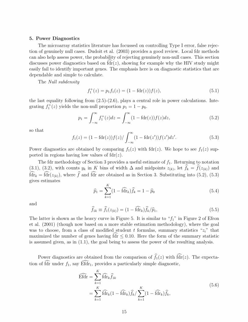
5. Power Diagnostics

The microarray statistics literature has focussed on controlling Type I error, false rejec-tion of genuinely null cases. Dudoit et al. (2003) provides a good review. Local fdr methodscan also help assess power, the probability of rejecting genuinely non-null cases. This sectiondiscusses power diagnostics based on fdr(z), showing for example why the HIV study mighteasily fail to identify important genes. The emphasis here is on diagnostic statistics that aredependable and simple to calculate.

The Null subdensity

f+1 (z) = p1f1(z) = (1 − fdr(z))f(z), (5.1)

the last equality following from (2.5)-(2.6), plays a central role in power calculations. Inte-grating f+

1 (z) yields the non-null proportion p1 = 1 − p0.

p1 =

∫ ∞

−∞f+

1 (z)dz =

∫ ∞

−∞(1 − fdr(z))f(z)dz, (5.2)

so that

f1(z) = (1 − fdr(z))f(z)/

∫ ∞

−∞(1 − fdr(z′))f(z′)dz′. (5.3)

Power diagnostics are obtained by comparing f1(z) with fdr(z). We hope to see f1(z) sup-ported in regions having low values of fdr(z).

The fdr methodology of Section 3 provides a useful estimate of f1. Returning to notation(3.1), (3.2), with counts yk in K bins of width ∆ and midpoints z(k), let fk = f(z(k)) and

fdrk = fdr(z(k)), where f and fdr are obtained as in Section 3. Substituting into (5.2), (5.3)gives estimates

p1 =K∑

k=1

(1 − fdrk)fk = 1 − p0 (5.4)

andf1k ≡ f1(z(k)) = (1 − fdrk)fk/p1, (5.5)

The latter is shown as the heavy curve in Figure 5. It is similar to “f1” in Figure 2 of Efronet al. (2001) (though now based on a more stable estimation methodology), where the goalwas to choose, from a class of modified student t formulas, summary statistics “zi” thatmaximized the number of genes having fdr ≤ 0.10. Here the form of the summary statisticis assumed given, as in (1.1), the goal being to assess the power of the resulting analysis.

Power diagnostics are obtained from the comparison of f1(z) with fdr(z). The expecta-

tion of fdr under f1, say Efdr1, provides a particularly simple diagnostic,

Efdr =K∑

k=1

fdrkf1k

=K∑

k=1

fdrk(1 − fdrk)fk/K∑

k=1

(1 − fdrk)fk,

(5.6)

15

Figure 5: Heavy curve proportional to non-null density estimate f1(z), (5.5), for HIV

study; light curve proportional to fdr(z). Points are thinned counts (5.9); a regression curve,dotted, has been fit directly to the thinned counts on the right.

the expected non-null false discovery rate. A small value of Efdr1, suggests good power, witha typical non-null case likely to show up on a list of interesting candidates for further study.

Table 3 shows Efdr1’s behavior in simulation (4.1), N = 1500. The situation is seen to be

favorable, with Efdr1, averaging only 0.23 or 0.29 using empirical or theoretical nulls (Section

7 explains the disparity between the two Efdr1 values). Moreover the individual Efdr1 valueswere reasonably stable, having standard deviations only 0.04 or 0.06. The empirical nullperforms well here, in contrast to Table 3.

empirical null theoretical null

p1 Efdr1 p1 Efdr1

mean: 0.76 .232 .085 .285stdev: .011 .040 .015 .060

coeffvar: .14 .17 .18 .21

Table 3: Means, standard deviations, and coefficients of variation of p1 and Efdr1 forN = 1500 case of Tables 1 and 2.

On the other hand, Efdr1 equals 0.45 for the HIV study (by necessity using the empiricalnull) so a typical non-null gene is likely to receive a substantial fdr estimate, high enough to

exclude it from the list of those having fdr ≤ 0.20.

16

The Efdr1, computations can be carried out separately to the left and right of z = 0by appropriately restricting the range of summation in the numerator and denominator of(5.6). Doing so gives Efdrleft = 0.51 and Efdrright = 0.35 for the HIV data. This says that itwill be particularly difficult to detect genes that underexpress in HIV-positive subjects.

Other moments or probabilities of fdr with respect to f1 are as simple to calculate asEfdr1, for example the standard deviation

Sd1 =

[K∑

k=1

fdr2

k · f1k − Efdr2

1

]1/2

, (5.7)

which equals 0.30 for the HIV data. The possibility of dependence among the zi’s does notbias estimates such as (5.6) or (5.7), though it increases their variability.

Going further, we can examine the entire distribution of fdr under f1. The heavy curvein Figure 6 shows the f1 cdf of fdr for the HIV study,

G(x) =∑ˆfdrk≤x

f1k

/ K∑k=1

f1k. (5.8)

Figure 6: Empirical cdf of fdr with respect to estimated non-null density f1. Heavy curveHIV study; Light curve first simulated sample (4.1), N = 1500. The simulated sample

displays greater power. Efdr1, equals 0.45 for HIV study, 0.23 for simulation.

For instance G(.2) = 0.27, so only 27% of the non-null cases are estimated to have fdr valuesless than 0.20. By contrast, the first of the N = 1500 simulated data sets from Table 1 isseen to have much greater power, with G(.2) = 0.64.

17

The limitations of the HIV study are forcefully illustrated by Figure 6: if we wish toreport 50% of the non-null cases then we must tolerate fdr values as high as 0.45 = G−1(.5),etc.

The thinned counts appearing in Figures 1, 2, and 5 are defined in terms of originalcounts yk as

y1k = (1 − fdrk) · yk. (5.9)

Since 1− fdrk is the probability of being non-null for a case in the kth bin, y1k is, nearly, anunbiased estimate of the number of non-null cases in bin k. We can use the thinned countsto carry out sample size power calculations for large-scale studies.

Traditional sample size calculations employ preliminary data to predict how large anexperiment will be required for effective power. Here we might ask, for instance, if doublingthe number of subjects in the HIV study would substantially improve its detection rate. Toanswer the question we assume a homoskedastic model for the z-values,

zi ∼ (µi, σ20), (5.10)

the notation indicating that zi has expectation µi, its “true score” and variance σ20, with

µi = 0 for the null cases. Sections 6 and 7 discuss the rationale for (5.10).

We imagine that c independent replicates of (5.10) are available for each case, fromwhich a combined statistic zi is formed,

zi =c∑

j=1

zij/√

c ∼ (√

c µi, σ20) (5.11)

This definition maintains the distribution of the null cases, zi ∼ (0, σ20), while moving the

non-null true scores away from zero 1 by factor√

c.

Consider a subset of the non-null cases in which the true scores have empirical meanand variance say (a, b2). A randomly selected z statistic “Z” from this subset has marginalmean and variance

Z ∼ (A,B2) = (a, b2 + σ20) (5.12)

according to (5.10), while the corresponding statistic “Z” from (5.11) has

Z ∼ (A, B2) = (√

c a, cb2 + σ20) (5.13)

Comparing (5.13) with (5.12) shows that the simple formula

Z =√

c A + d(Z − A), [d2 = c − (c − 1)σ20/B

2], (5.14)

gives Z the correct mean and variance.

From the thinned counts (5.9) on the right side of Figure 5 we estimate

A =

∑z(k)y1k∑

y1k

= 2.23 and B =

[∑z2(k)y1k∑y1k

− A2

] 12

= 0.87, 5.15)

18

the sums being over z(k) > 0. Then (5.14), with σ0 = 0.735 from the empirical null, describeshow the right-side non-null zi’s might transform under increased sample sizes (5.11). Asimilar calculation applies on the left, while the null scores, of which there are yk − y1k inthe kth bin, would remain unchanged.

Table 4 reports on Efdr1, (5.6), for hypothetical transformed data sets having c =1, 1.5, 2, and 2.5. We see that doubling the number of subjects, from 4 to 8 in each group,would reduce Efdr1 from 0.45 to 0.28, a substantial improvement. Table 3 involves a consid-erable amount of speculation, more so than diagnostics (5.6)-(5.8), but power computationsare traditionally speculative; the calculations here, involving just means and variances, arefashioned to minimize the amount of parametric modeling.

The dotted curve on the right side of Figure 5 is a cubic Poisson GLM fit directly to thethinned counts y1k; that is, we assume

y1kind∼Po(ν1k), (5.16)

for log(ν1k) a cubic polynomial in the bin midpoints z(k), say

(log ν1k) = X1β, (5.17)

with X1 a K1 ×m1 structure matrix; K1 is the number of bins involved and m1 the numberof parameters, m1 = 4 here.

#Subjects 4-4 6-6 8-8 10-10

Efdr1: 0.45 0.33 0.28 0.22

Table 4: Estimated values of Efdr1, for expanded versions of HIV study; doubling thestudy, to 8 subjects each in the two groups reduces Efdr1 from 0.45 to 0.28.

The usual GLM estimate of covariance for β is

G−11 = (X ′

1 diag (ν1k)X1)−1. (5.18)

However this leads to an overestimate under model (3.1), because y1k = (1 − fdrk)yk hasvariance about (1 − fdrk)ν1k, less than the Poisson value ν1k assumed in (5.16). A moreaccurate approximation is

Cov(β) = G−11 [X ′

1 diag ((1 − fdrk)ν1k)X1)−1G−1

1 , (5.19)

Estimating f1 directly from the thinned counts is appealing since it does not involve aglobal fit to all N cases, as does (5.5), a fact we took advantage of in using only a cubicmodel for the dotted curve. It did not make much difference to the HIV analysis though,nor did simply replacing f1k with y1k in (5.6)-(5.8).

19

6. The Non-Null Distribution of z-values

A key assumption of our fdr estimation methodology was the smooth nature of the z-value mixture density f(z). This section discusses a useful approximation for the distributionof z-values, null or non-null,

Z∼N(µ, σ2µ), (6.1)

where Z represents a generic z-value, µ its expectation, “∼” indicates second order accu-racy with distributional errors of order O(n−1) in the usual repeated sampling context, and

σµ = 1 +O(n− 12 ). The smoothness assumption is justified by (6.1), which represents f(z) as

a well-controlled mixture of normal densities.

Figure 7 illustrates (6.1) for transformed t-statistics (1.1). We suppose that ti has anoncentral t distribution, noncentrality θ and degrees of freedom ν,

ti ∼θ + W

S1/2[W ∼ N(0, τ) independent of s ∼ τx2

ν/ν]. (6.2)

Figure 7: Density of z-value (1.1) when ti is non-central t variate, 6 degrees of freedom;non-centrality parameter θ = .5, 1.5, 2.5, 3.5, 4.5 left to right. Means 0.42, 1.35, 2.04, 2.56,2.96; stdevs 0.98, 0.88, 0.75, 0.65, 0.58. Dotted curves are corresponding normal densities.

By definition zi ∼ N(0, 1) in the null case θ = 0. (For the calculations of this sectionwe are ignoring the failure of the theoretical null in Figure 4.) Figure 7 shows the densityof zi = Φ−1(F6(ti)) for θ = .5, 1.5, · · · , 4.5. We see σµ declining from 1 at θ = 0 to 0.58 atθ = 4.5, while the normality claimed in (6.1) is nicely maintained.

Relationship (6.1) can be verified in a wide variety of situations. Suppose Z is based on

testing H0 : θ = 0 for a summary statistic θ having cdf Fθ,

Z = Φ−1(F0(θ)). (6.3)

20

We assume that θ behaves asymptotically like a maximum likelihood estimate in terms ofa notional sample size “n”, its bias, standard deviation, skewness, and kurtosis having theappropriate orders of magnitude,

θ − θ ∼ (Bθ/n, Cθ/√

n,Dθ/√

n,Eθ/n); (6.4)

Bθ, Cθ, Dθ, and Eθ are smooth bounded functions of θ and n.

Following Sections 3-5 of Efron (1987), particularly Theorem 1, there exists a monotone

increasing transformation φ = g(θ), φ = g(θ), 0 = g(0), such that

φ ∼ φ + (1 + aφ)(W − z0), (6.5)

with W ∼ N(0, 1) and a and z0, the “acceleration” and “bias-correction” constants, each of

order O(n− 12 ). At θ = φ = 0 we have φ ∼ N(−z0, 1), implying Z = φ + z0. Then (6.4) gives

Z ∼ φ(1 − az0) + (1 + aφ)W ∼ N(φ, (1 + aφ)2), (6.6)

(az0 = O(n−1) being ignorably small) verifying (6.1) with µ = φ and

σµ = 1 + aµ. (6.7)

The acceleration constant “a” determines how quickly σµ departs from σ0 = 1. Efron (1987)derives approximation a = skew (�0)/6, in terms of the score function �0 at θ = 0.

As an example suppose we observe scaled one-sided exponential varieties,

y1, y2, . . . , ynind∼θG1 [Pr{G1 < x} = 1 − e−x], (6.8)

so that θ = y ∼ θ Gamman/n. For n = 10, and for any choice of the null hypothesisH0 : θ = θ0, the score function approximation gives a = 1/(3

√10) = .1054, while direct

numerical computation yielded

dσµ

dµ

∣∣∣∣∣θ0

= .1049; (6.9)

σµ varied on the range [0.5, 1.5] for µ in ±5. The normal approximation is just as impressivehere as in Figure 7.

The gist of (6.1), (6.7) is that as µ departs from zero by amount O(1), σµ changes by

O(n− 12 ) while normality decays by only O(n−1). The student t example of Figure 7 is not

included in development (6.4)-(6.7), because of the nuisance parameter τ in (6.2), but in factshowed even greater accuracy for (6.1). This can be verified using the diagnostic function inEfron (1982).

Going further, we can consider the situation where Z is the z-value for a single parameterin a multiparameter family. A promising conjecture is that (6.1), (6.7) holds in multiparam-eter exponential families if z-values are obtained via the ABC method, DiCiccio and Efron(1992). Section 4 of Efron (1988) discusses a variant of (6.1) applying to sequential sampling.

21

Model (6.1) can be used to sharpen the sample size calculations of Section 5. Consider asubset of cases, say the non-null cases on the right side of Figure 5, and let g(µ) represent theempirical distribution of their true scores µi. Formulas (5.12)-(5.15) tacitly involve estimating

g(µ) : (A, B2), the mean and variance of the thinned counts, give estimates (a, b2) for themean and variance of g(µ), (5.12), which depend on the homoskedastic model (5.10). Insteadwe could begin with (6.1) and directly deconvolve the thinned counts to obtain g(µ). Doingso made little difference to Table 4. However g(µ) can be useful in its own right, in particularfor estimating the Bayes posterior distribution of true score µi given zi.

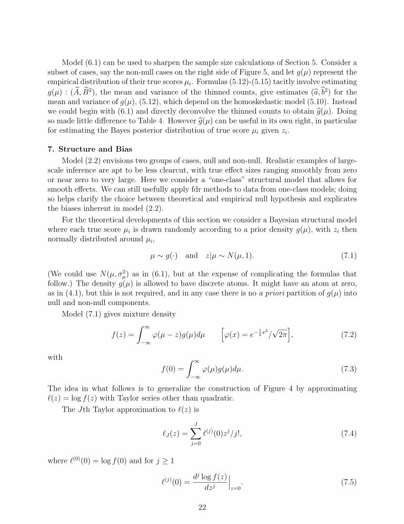
7. Structure and Bias

Model (2.2) envisions two groups of cases, null and non-null. Realistic examples of large-scale inference are apt to be less clearcut, with true effect sizes ranging smoothly from zeroor near zero to very large. Here we consider a “one-class” structural model that allows forsmooth effects. We can still usefully apply fdr methods to data from one-class models; doingso helps clarify the choice between theoretical and empirical null hypothesis and explicatesthe biases inherent in model (2.2).

For the theoretical developments of this section we consider a Bayesian structural modelwhere each true score µi is drawn randomly according to a prior density g(µ), with zi thennormally distributed around µi,

µ ∼ g(·) and z|µ ∼ N(µ, 1). (7.1)

(We could use N(µ, σ2µ) as in (6.1), but at the expense of complicating the formulas that

follow.) The density g(µ) is allowed to have discrete atoms. It might have an atom at zero,as in (4.1), but this is not required, and in any case there is no a priori partition of g(µ) intonull and non-null components.

Model (7.1) gives mixture density

f(z) =

∫ ∞

−∞ϕ(µ − z)g(µ)dµ

[ϕ(x) = e−

12x2

/√

2π], (7.2)

with

f(0) =

∫ ∞

−∞ϕ(µ)g(µ)dµ. (7.3)

The idea in what follows is to generalize the construction of Figure 4 by approximating�(z) = log f(z) with Taylor series other than quadratic.

The Jth Taylor approximation to �(z) is

�J(z) =J∑

j=0

�(j)(0)zj/j!, (7.4)

where �(0)(0) = log f(0) and for j ≥ 1

�(j)(0) =dj log f(z)

dzj

∣∣∣z=0

. (7.5)

22

The sub-densityf+

0 (z) = e�J (z) (7.6)

matches f(z) at z = 0 (a convenient use of the zero assumption) and leads to an fdr expressionas in (2.6),

fdr(z) = e�J (z)/f(z). (7.7)

Larger choices of J match f+0 (z) more accurately to f(z), increasing ratio (7.7); the inter-

esting z-values, those with small fdr’s, are pushed farther away from zero as we allow moreof the data structure to be explained by the null density.

The Bayesian model (1.1) provides a helpful interpretation of the derivatives �(j)(0):

Lemma 2 The derivative �(j)(0), (7.5), is the jth cumulant of the posterior distributionof µ given z = 0, except that �(2)(0) is the second cumulant minus 1. Thus

�(1)(0) = E0 and − �(2)(0) = V0, (7.8)

where E0 and V0 ≡ 1 − V0 are the posterior mean and variance of µ given z = 0.

Proof We have

�(z) = log∫ ∞−∞

e−12 (µ−z)2

√2π

g(µ)dµ

= −12z2 + log f(0) + log

∫ ∞−∞ ezµ[ϕ(µ)g(µ)/f(0)]dµ.

(7.9)

Notice that m(z) ≡∫ ∞−∞ ezµ[ϕ(µ)g(µ)/f(0)]dµ is the moment generating function of the

probability density ϕ(µ)g(µ)/f(0),

djm(z)

dzj|z=0 =

∫ ∞

−∞µj ϕ(µ)g(µ)

f(0)dµ, (7.10)

the last expression also being the posterior jth moment of µ given z = 0. The usualrelationship between moments and cumlants, applied to the function �(z) + 1

2z2 − log f(0),

verifies the Lemma.

For J = 0, 1, 2, formulas (7.7), (7.8) yield simple expressions for p0 and f0(z) in termsof f(0), E0, and V0. These are summarized in Table 5 (with p0 obtained through definition(2.4),

p0 =[ ∫ ∞

−∞f+

0 (z)dz]−1

. ) (7.11)

Formulas are also available for Fdr(z), (2.8).

The choices J = 0, 1, 2 in Table 5 result in a normal null density f0(z), the only differencebeing the means and variances. Going to J = 3 allows for an asymmetric choice of f0(z);from (7.9) and the Lemma,

fdr(z) =f(0)

f(z)eE0z−V0z2/2+S0z3/6, (7.12)

23

J : 0 1 2

p0: f(0)√

2π f(0)√

2π eE20/2 f(0)

√2πV0

eE20/2V0

f0(z): N(0, 1) N(E0, 1) N(E0/V0, 1/V0)

fdr(z): f(0)e−z2/2

f(z)f(0)eE0z−z2/2

f(z)f(0)eE0z−V0z2/2

f(z)

Table 5: Expressions for p0, f0 and fdr, first three choices of J in (7.6), (7.7); numeratorof fdr(z) is f+

0 (z). J = 0 gives theoretical null, J = 2 empirical null; f(z) from (7.2).

p0 δ σ p(theo)0 E0 V0

Model (7.13): 0.916 0.013 1.01 0.906 0.012 0.022Model (7.14): 0.918 0.018 1.13 0.821 0.014 0.223

Table 6: p0 and f0(z) from Table 5; δ and σ mean and standard deviation of empiricalnull, Top line Model (7.13), as used in simulation study; Bottom line Model (7.14).

where S0 is the posterior third central moment of µ given z = 0 in model (7.1). Theprogram locfdr uses a variant, the “split normal”, to model asymmetric null densities withthe exponent of (7.12) replaced by a quadratic spine in z.

Lemma 2 bears on the difference between empirical and theoretical nulls. Suppose thatthe probability mass of g(µ) occurring within a few units of the origin is concentrated in anatom at µ = 0. Then the posterior mean and variance (E0, V0) of µ given z = 0 will be near0, making (E0, V0) = (0, 1). In this case the empirical null (J = 2) will approximate thetheoretical null (J = 0). Otherwise the two nulls will differ; in particular, any mass of g(µ)

around zero increases V0, swelling the standard deviation (1 − V0)− 1

2 of the empirical null.

Model (4.1), used for the simulation study, has

g(µ) = 0.9 · I0(µ) + 0.1 · ϕ3,1(µ), (7.13)

I0(µ) a unit atom at µ = 0, which gives mixture density f(z) = 0.9 · ϕ0,1(z) + 0.1 · ϕ3,√

2(z)according to (7.1). The top line of Table 6 shows p0 and f0(z) for (7.13), as calculated fromTable 5. This amounts to having N equal infinity in Table 2 (except for matching f+

0 (z) tof(z) at z = 0 in (7.6) instead of averaging over the central third of f as in locfdr). We seesmall biases away from f+

0 (z) = 0.9 ·ϕ0,1(z) : p0 exceeds 0.9, more so for the empirical null,and (δ, σ) is slightly distorted from (0, 1).

Bias is more apparent in the left panel of Figure 8, which plots f1(z) = (1− fdr(z)) ·f(z)as calculated from Table 5. The left tail of f1(z) is pushed away from zero compared to thenominal f1 density ϕ3,

√2(z), again more so for the empirical null. The zero assumption is

the culprit here, as mentioned before, since in fact ϕ0,1 and ϕ3,√

2 overlap somewhat. Theempirical’s greater rightward shift, toward smaller fdr values, accounts for its smaller Efdr1

average in Table 3: computing Efdr1 =∫

fdr(z) ·f1(z)dz according to Table 5 gives 0.245 for

24

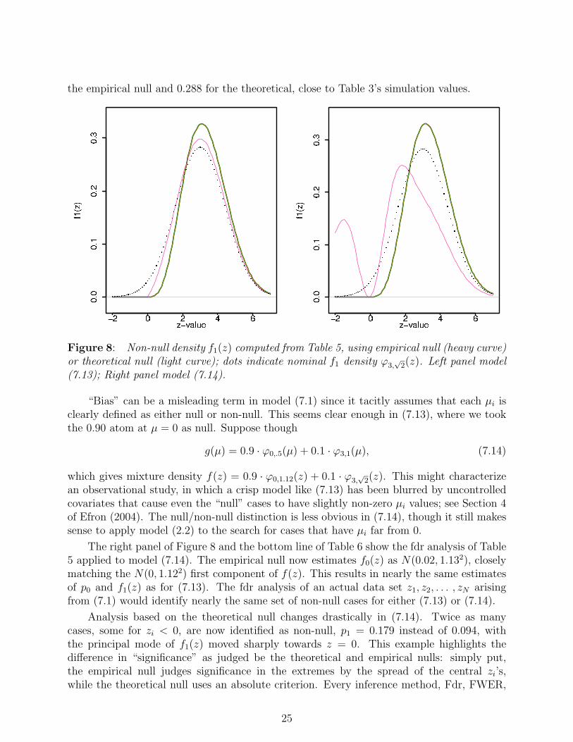
the empirical null and 0.288 for the theoretical, close to Table 3’s simulation values.

Figure 8: Non-null density f1(z) computed from Table 5, using empirical null (heavy curve)or theoretical null (light curve); dots indicate nominal f1 density ϕ3,

√2(z). Left panel model

(7.13); Right panel model (7.14).

“Bias” can be a misleading term in model (7.1) since it tacitly assumes that each µi isclearly defined as either null or non-null. This seems clear enough in (7.13), where we tookthe 0.90 atom at µ = 0 as null. Suppose though

g(µ) = 0.9 · ϕ0,.5(µ) + 0.1 · ϕ3,1(µ), (7.14)

which gives mixture density f(z) = 0.9 · ϕ0,1.12(z) + 0.1 · ϕ3,√

2(z). This might characterizean observational study, in which a crisp model like (7.13) has been blurred by uncontrolledcovariates that cause even the “null” cases to have slightly non-zero µi values; see Section 4of Efron (2004). The null/non-null distinction is less obvious in (7.14), though it still makessense to apply model (2.2) to the search for cases that have µi far from 0.

The right panel of Figure 8 and the bottom line of Table 6 show the fdr analysis of Table5 applied to model (7.14). The empirical null now estimates f0(z) as N(0.02, 1.132), closelymatching the N(0, 1.122) first component of f(z). This results in nearly the same estimatesof p0 and f1(z) as for (7.13). The fdr analysis of an actual data set z1, z2, . . . , zN arisingfrom (7.1) would identify nearly the same set of non-null cases for either (7.13) or (7.14).

Analysis based on the theoretical null changes drastically in (7.14). Twice as manycases, some for zi < 0, are now identified as non-null, p1 = 0.179 instead of 0.094, withthe principal mode of f1(z) moved sharply towards z = 0. This example highlights thedifference in “significance” as judged be the theoretical and empirical nulls: simply put,the empirical null judges significance in the extremes by the spread of the central zi’s,while the theoretical null uses an absolute criterion. Every inference method, Fdr, FWER,

25

permutation, Bonferroni, and not just fdr, yields doubtful results if model (7.14) is analyzedin terms of the theoretical null.

Summary The local false discovery rate methodology developed in Sections 3 and 5 isbased on empirical Bayes analysis of the simple two-class model (2.2); fdr calculations pro-vide both size and power estimates, while requiring a minimum of frequentist or Bayesianmodeling assumptions. The methodology applies to large-scale situations, with hundreds ofinference problems considered simultaneously, perhaps at least a thousand if the theoreticalnull hypothesis is unsatisfactory. A closed form error analysis of fdr estimation, developed inSection 4, is available when the inference problems are independent. Even when the two-classmodel is dubious, as discussed in Section 7, fdr methods can still be informative, though nowthey are more likely to require empirical estimation of the null hypothesis. All calculationsare carried through using standard Poisson GLM software; program locfdr is available fromthe R library CRAN.

26

References

Allison, D., Gadbury, G., Heo, M., Fernandez, J., Lee, C.K., Prolla, T., and Weindruch, R.(2002), “A mixture model approach for the analysis of microarray gene expression data”,Computational Statistics and Data Analysis 39, 1-20.

Aubert, J., Bar-hen, A., Daudin, J., and Robin, S. (2004), “Determination of the differen-tially expressed genes in microarray experiments using local FDR”, BMC Bioinformatics5:125.

Benjamini, Y. and Hochberg, Y. (1995), “Controlling the false discovery rate: a practicaland powerful approach to multiple testing”, Journal of the Royal Statistical Society, Ser.B, 57, 289-300.

Broberg, P. (2005), “A new estimate of the proportion unchanged genes in a microarrayexperiment”, Genome Biology 5:p10.

DiCiccio, T. and Efron, B. (1992), “More accurate confidence intervals in exponential fami-lies”, Biometrika 79, 231-45.

Do, K.A., Mueller, P., and Tang, F. (2003), “A nonparametric Bayesian mixture model forgene expression”, mbi.osu.edu/2004/ws1materials/do.pdf. To appear Jour. Roy. Stat.Soc. C.

Dudoit, S., van der Laan, M., and Pollard, K. (2004), “Multiple testing, part I: Single stepprocedures for the control of general Type I error rates”, Statistical Applications in Genet-ics and Molecular Biology 3, article 13: http://www.bepress.com/sagmb/vol3/iss1/art13.

Dudoit, S., Shaffer, J., and Boldrick, J. (2003), “Multiple hypothesis testing in microarrayexperiments”, Statistical Science 18, 71-103.

Efron, B. (2004), “Large-scale simultaneous hypothesis testing: the choice of a null hypoth-esis”, JASA 99, 96-104.

Efron, B., and Tibshirani, R. (2002), “Empirical Bayes methods and false discovery rates formicroarrays”, Genetic Epidemiology 23, 70-86.

Efron, B. and Gous, A. (2001), “Scales of evidence for model selection: Fisher versus Jef-freys”, Model Selection IMS Monograph 38, 208-256.

Efron, B., Tibshirani, R., Storey, J. and Tusher, V. (2001), “Empirical Bayes analysis of amicroarray experiment”, Journal of the American Statistical Association 96, 1151-1160.

Efron, B. and Tibshirani, R. (1996), “Using specially designed exponential families for densityestimation”, Annals Stat. 24, 2431-61.

Efron, B. (1988), “Three examples of computer-intensive statistical inference”, Sankhya 50,338-362.

Efron, B. (1987), “Better bootstrap confidence intervals”, Jour. Amer. Stat. Assn. 82,171-95.

27

Efron, B. (1982), “Transformation theory: how normal is a family of distributions?”, AnnalsStat. 10, 323-339.

Genovese, C. and Wasserman, L. (2004), “A stochastic process approach to false discoverycontrol”, Annals Stat. 32, 1035-1061.

Gottardo, R., Raftery, A., Yeung, K., and Bumgarner, R. (2004), “Bayesian robust inferencefor differential gene expression in microarrays with multiple samples”, Dept. Statistics,U. Washington technical report, raph@stat.washington.edu

Heller, G. and Qing, J. (2003), “A mixture model approach for finding informative genes inmicroarray studies”, Unpublished.

Johnstone, I. and Silverman, B. (2004), “Needles and straw in a haystacks: empirical Bayesapproaches to thresholding a possibly sparse sequence”, Annals Stat. 32, 1594-1649.

Kendziorski, C., Newton, M., Lan, H., and Gould, M. (2003), “On parametric empiricalBayes methods for comparing multiple groups using replicated gene expression profiles”,Stat. in Medicine 22, 3899-3914.

Kerr, M., Martin, M., and Churchill, G. (2000), “Analysis of variance in microarray data”,Jour. Computational Biology 7, 819-837.

Lee, M.L.T., Kuo, F., Whitmore, G., and Sklar, J. (2000), “Importance of replication inmicroarray gene expression studies: statistical methods and evidence from repetitive cDNAhybridizations”, Proc. Nat. Acad. Sci. 97, 9834-38.

Liao, J., Lin, Y., Selvanayagam, Z., and Weichung, J. (2004), “A mixture model for esti-mating the local false discovery rate in DNA microarray analysis”, Bioinformatics 20,2694-2701.

Newton, M., Noveiry, A., Sarkar, D., and Ahlquist, P. (2004), “Detecting differential geneexpression with a semiparametric hierarchical mixture model”, Biostatistics 5, 155-176.

Newton, M., Kendziorski, C., Richmond, C., Blattner, F., and Tsui, K. (2001), “On differen-tial variability of expression ratios: improving statistical inference about gene expressionchanges from microarray data, Jour. Comp. Biology 8, 37-52.

Pan, W., Lin, J., Le, C. (2003), “A mixture model approach to detecting differentiallyexpressed genes with microarray data”, Functional & Integrative Genomics 3, 117-24.

Pollard, K. and van der Laan, M. (2003), “Resampling-based multiple testing: asymptoticcontrol of type I error and applications to gene expression data”, U.C. Berkeley Biostatis-tics working paper 121; http://www/bepress.com/ucbiostat/paper121

Pounds, S. and Morris, S. (2003), “Estimating the occurrence of false positions and false neg-atives in microarray studies by approximating and partitioning the empirical distributionof the p-values”, Bioinformatics 19, 1236-42.

Storey, J., Taylor, J., and Siegmund, D. (2004), “Strong control, conservative point esti-mation and simultaneous conservative consistency of false discovery rates; a unified ap-proach”, Jour. Royal Stat. Soc. B 66, 187-206.

28

Storey, J. (2002), “A direct approach to false discovery rates”, Journal of the Royal StatisticalSociety, Ser. B, 64, 479-498.

Tusher, V., Tibshirani, R., and Chu, G. (2001), “Significance analysis of microarrays appliedto transcriptional responses to ionizing radiation”, Proc. Nat. Acad. Sci. 98, 5116-21.

Westfall, P. and Young, S. (1993), Resampling-based multiple testing: examples and methodsfor p-value adjustment, New York, Wiley.

29