LOAN DOCUMENTPHOTOGRAPH THIS SHEET

LEVEL INVENTORY

DOCUMuT IDENTIFICATION

HA A

I*STPIIBUTiON g~P~iNL.;' AA

S A 0ppo,,ed lor puliUc re.la,'x,

Dwftbufton Unirnited D

DISTRIBUTION STATEMENT LAtI[LS[ FORE

"TI" GRA&T E:)TIC TRAC E3:%ANNOUNCED 03 ." "J1,STII ICATION 4

JUN 2 4 199Kij" W

DISTRIBUTION/

AvAll AR1h ITY CODES

o/ DATE A'CESSIONED

I)ISTRIBUTION STAMP RE

DATE RETURNED

92-16510,z, 1111 111 11 ill 1111 11 Hll 1111 IIllllDATE RECEIVED IN DTIC REGISTERED OR CERTIFIED NUMBER

PHOTOGRAPH THIS SHEET AND RETURN TO DTIC.FDACDTIC 70A DIr PROCESSING SHEETTIS MAY BE USLD N

7Troc 1 FXHAUSTED

LOAN DOCUMENT

1 r o e ed L ng s

of the

Fifteenth Annual Gravity Gradiometry Conference

United States Air Porce AcademyColorado Springs, Colorado

11-13 February 1987

VOLUME II

Compiled By:

copt Vishnu V.. Nevrekar,. USAF

Earth Sciences Division!,USAF Geophysics laboratoryHanscom AFB, MA 01731

DISCLAIMER NOTICE

THIS DOCUMENT IS BEST

QUALITY AVAILABLE. THE COPY

FURNISHED TO DTIC CONTAINED

A SIGNIFICANT NUMBER OF

PAGES WHICH DO NOT

REPRODUCE LEGIBLY.

ABOUT THESE PROCEEDINGS .

Due to the large number of papers presentn at the Conference, I havedivided the proceedings into two manageable volumes. At the beginning ofeach volume is a list of all papers contained in both volumes, in actualorder of presentation at the Conference. This is also the sequence of thepublished papers within these proceedings.

For the sake of completeness, both volumes contain the Attendees List,

Conference Agenda, Lists of Papers, Conference History, Acknowledgmentsand this explanation.

Every paper is preceded by an abstract in a standard format. Some papersmay also have the original abstract included. Further, you may recall theQ&A session we had at the end of each presentation. In cases where atechnical interchange did take place, the questions and answers aredocumented at the end of each pertinent paper. Every paper did not havea Q&A session, and I have included all Q&A sheets that were handed to meat the end of each presentation. Except for a few minor editorial changes,the information on these sheets has not been significantly altered.Obviously, these sheets are as "good" as the inputs you provided.

In summary, I hope the above explanation was helpful. I have done what Iconsider to be a thorough job of collecting and checking all theinformation for these proceedings. Errors will occur, however, and while

W I will entertain any comments and criticisms on this issue, these

proceedings will stand as published.

Thank you for your participation, and your patience!

Capt Vishnu V. Nevrekar November 1987Earth Sciences Division

USAF Geophysics Laboratory

Hanscom AFB, MA 01731

S

ABOUT THE GRAVITY GRADIOMETRY ONFERENCE .....

The First Gravity Gradiometry Conference was held at the Air Force CambridgeResearch Laboratory (AF(RL, now AFGL) in 1973. Its purpose was to providea forum to evaluate and compare the efforts of three vendors (Charles StarkDraper Lab, Hughes Research Lab and Bell Aerospace Textron) in still-emergingareas of gravity gradiometry. About 15 people attended, most of them from thecompanies mentioned above or the Terrestrial Sciences Division at AFCRL. Incontrast, the 1987 Conference had a guest list of 70 plus attendees, withparticipation from academia (foreign and domestic), private industry and

government. The papers presented were not restricted to gradiometry alone.Indeed, the scope of this annual event has broadened considerably since 1973.

With the exception of the first two conferences, all the others have beenheld at the US Air Force Academy in Colorado Springs, Colorado. The Geodesyand Gravity Branch of the Earth Sciences Division of the Air Force GeophysicsLaboratory (AFGL), Hanscom AFB, Massachusetts, has always organized the event,which usually takes place around the second week in February. This trend isexpected to continue.

If you are not already on our mailing list and would like to attend the1988 Conference, or if you have any questions, please write to:

Ms Claire McCartneyA FUL LWHanscom AFB, MA 01731

Due to space constraints, we restrict the size of our Conferences to about 75people. Attendance will generally be on a "first-come, first-served basis" oncethe completed registration forms are returned to us. We shall mail these forms

later this year.

While we have a limited number of copies of the proceedings for non-attendeesof the 1987 Conference, copies of proceedings for prior years are not available.Also, we appreciate any comments or suggestions you may have regarding this

document.

0

ACKNOWLEDGMENTS SWe couldn't possibly organize a conference the scope and size of our forumwithout some very diligent "behind-the-scenes" work by a few outstandingindividuals. We would like to recognize their efforts and thank them fortheir support throughout the planning and execution of the 1987 GradiometryConference.

We are indebted to the Directorate of Protocol at the US Air Force Academyfor allowing us to host the Conference there these past 13 years. Ms NancyGass was the liaison officer from the Directorate, and we gratefullyacknowledge her assistance in handling all the conference arrangements,including hotel accomodation for the attendees, transportation for theConference and NORAD/CSOC tours, luncheons during the conference and the"mixers" later in the evening, all of which were set up with great skilland professionalism.

Also, we acknowledge the outstanding efforts of TSgt Kent Droz, USAF, of theCommunity Relations Division at HQ NORAD, who arranged tours of the CheyenneMountain Complex (04C) and the Consolidated Space Operations Center (CSOC)at Falcon AFS. These tours gave the conference attendees a first-hand lookat the complex space defense environment.

Next, we thank all the speakers for taking the time to compile and presenttheir papers for the benefit of the Conference attendees. As always, the broadmix of topics went a long way towards making the Conference an intellectuallystimulating event. Indeed, the high quality of the research material presented..made" this Conference.

Finally, we thank Col J.R. Johnson, then Commander, AFGL, Dr Donald H. Eckhardt,Director, Earth Sciences Division and Dr Thomas P. Rooney, Chief, Geodesyand Gravity Branch, without whose support and guidance this Conference couldnot have been held.

4

Alphabetical Listing of Conference Participants

(Name Organization

*Georges Balmino C.N.E.S./Bureau Gravimetrique International (FR)

Anthony Barringer Barringer Resources, Inc

*Hans Baussus Von Luetzow US Army Engineer Topographic Laboratory

Don Benson Dynamics Research Corporation

Ed Biegert Shell Development Corporation

John Binns BP Minerals International, Ltd (UX)

*Sam Bose Applied Science Analytics, Inc

*Carl Bowin Woods Hole Oceanographic Institution

John Brozena Naval Research Laboratory

Marcus Chalona US Naval Oceanographic Office

Lindrith Cordell US Geological Survey

Ronald Davis Northrop Electronics Division

O Mark Dransfield University of Western Australia (AUS)

Donald Eckhardt USAF Geophysics Laboratory

Michael Ellett USAF Space Division

Harry Emrick Consultant

John Fett LaCoste and Romberg Gravity Meters, Inc

Charles Finley National Aeronautics and Space Administration

Thomas Fischetti Technology Management Consultants, Inc

James Fix Teledyne Geotech

Guy Flanagan Standard Oil Production Company

*Rene Forsberg Geodetic Institute (DEN)

Capt Terry Fundak USAF Geophysics Laboratory

*David Gleason USAF Geophysics Laboratory

Rob Goldsborough USAF Geophysics Laboratory

Name Organization

*John Graham Defense Mapping Agency

Andrew Grierson Bell Aerospace Textron

Michael Hadfield Honeywll, Inc

Richard Hansen Colorado School of Mines

Chris Harrison Geodynamics Corporation

Ray Hassanzadeh McDonnell Douglas

*Warren Heller The Analytic Sciences Corporation

Howard Heuberger Johns Hopkins University

George Hinton Consultant

Albert Hsui USAF Geophysics Laboratory

Gene Jackson McDonnell Douglas

Christopher Jekeli USAF Geophysics Laboratory

*Albert Jircitano Bell Aerospace Textron

Col J.R. Johnson Commander, USAF Geophysics Laboratory

J. Edward Jones USAF Intelligence Service

J. Latimer Johns Hopkins University

Andrew Lazarewicz USAF Geophysics Laboratory

Thomas Little US Naval Oceanographic Office

*Dan Long Eastern Washington University

James Lowery III Rockwell International

Charles Martin University of Maryland Research Foundation

*Bahram Mashhoon University of Missouri

*Ernest Metzger Bell Aerospace Textron

*M. Vol Moody University of Maryland

*Ian Moore University of Queensland (AUS)

ILt Vishnu Nevrekar USAF Geophysics Laboratory

*Ho Jung Paik University of Maryland

Name Organization

Mtaj John Prince USAF Office of Scientific Research

*Richard Rapp Ohio State University

Richard Reineman GWR Instruments

*Jean-Paul Richard University of Maryland

Thomas Rooney USAF Geophysics Laboratory

Alan Rufty Naval Surface Weapons Center

Alton Schultz AMOCO Production Company

*Michael Sideris University of Calgary (CAN)

Ted Sims Naval Surface Weapons Center

Randall Smith Defense Mapping Agency

*David Sonnabend CALTEaI/Jet Propulsion Laboratory

Milton Trageser Charles Stark Draper Laboratory

Gary Tuck University of Queensland (AUS)

Herbert Valliant LaCoste and Romberg Gravity Meters, Inc

* Robert Valska Defense Mapping Agency

*Frank van Kann University of Western Australia (AUS)

Richard Wold TerraSense, Inc

Robert Ziegler Defense Mapping Agency

*Alan Zorn Dynamics Research Corporation

Paul Zucker Johns Hopkins University

* Denotes Speaker at ConferenceI

Fifteenth Gravity Gradiometer ConferenceUnited States Air Force Academy

Colorado Springs, Colorado

ONFERENCE AGENDA

Tuesday, 10 February 1987

1900 - 2200 - Pre-Conference Get-Together at Hilton InnEarly Registration

Wednesday, I. February 1987

0700 - Depart Hilton Inn for Fairchild Hall

0730 - Registration - 3rd floor Fairchild Hall, South End

0745 - Welcome/Introduction - Capt Terry J. Pindak

0815 - Presentation by Dr. Georges Balmino of the ONERA (Office Nationald'Etudes et de Recherches Aerospatiales).

"GRADIO Project: A SGG Mission Based on Microaccelerometers"

0845 - Presentation by Dr. G. Ian Moore of the University of Queensland.

"A Mercury Manometer Gravity Gradiometer"

0900 - Presentation by Mr. Ernest H. Metzger of Bell Aerospace Textron.

"Bell Aerospace Gravity Gradiometer Survey System (GGSS) - ProgramReview"

0925 - Presentation by Dr. Frank J. van Kann of the University of WesternAustralia.

"A Prototype Superconducting Gravity Gradiometer for GeophysicalExploration"

0952 - Presentation by Dr. Warren G. Heller of The Analytic Sciences Corp.

"Gravity Gradiometer Survey System (GGSS) Data Processing and DataUse"

1016 - Break

1035 - Presentation by Mr. Al Jircitano of Bell Aerospace Textron.

"Self-Gradient Calibration of the GGSS in a C-130 Aircraft"

1058 - Presentation by Dr. Sam C. Bose of Applied Sciences Analytics, Inc.

"Gravity Gradiometer Data Processing Using the Karhunen-LoeveMethod"

1120 - Presentation by Mr. David M. Gleason of the Air Force GeophysicsLaboratory.

"Numerically Deriving the Kernels of an Integral Predictor YieldingSurface Gravity Disturbance Components from Airborne Gradient Data"

1130 - Presentation by Mr. Al Jircitano of Bell Aerospace Textron.

"Stage II Simulation Results Using the NSWC Synthetic GravityField"

1150 - Depart Fairchild Hall for USAFA Noncommissioned Officers'(NOD) Club

1200 - Lunch - USAFA NO Qub

1245 - Depart ND Club for Fairchild Hall

1330 - Presentation by Dr. Richard H. Rapp of Ohio State University.

"Gradient Information in New High Degree Spherical HarmonicExpansions"

1354 - Presentation by Mr. John J. Graham of the Defense Mapping AgencyAerospace Center.

"The Effect of Topography on Airborne Gravity Gradiometer Data"

1357 - Presentation by Mr. Mike Sideris of the University of Calgary.

"Effect of Terrain Representation, Grid Spacing, and Flight Altitudeon Topographic Corrections for Airborne Gradiometry"

1417 - Presentation by Dr. Rene Forsberg of Geodetic Institute (Denmark)(Oirrently at the University of Calgary, Canada).

"Topographic Effects in Airborne Gravity Gradiometry"

1434 - Presentation by Dr. Alan H. Zorn of Dynamics Research Corporation.

"Observability of Laplace's Equation Using a Torsion-TypeGravity Gradiometer"

1510 - Break

1530 - Presentation by Dr. Carl Bowin of Woods Hole Oceanographic Institute.

"Ratios of Gravity Gradient, Gravity, and Geoid for Determination ofCrustal Structure"

1550 - Presentation by Dr. Rene Forsberg of Geodetic Institute (Denmark).

"Combining Gravity Gradiometry with Other ExplorationMethods for Geophysical Prospecting"

1600 - Presentation by Dr. Rene Forsberg of Geodetic Institute (Denmark).

"Computation of the Gravity Vector from Torsion Balance Data in S.Ohio"

1615 - Presentation by Dr. Hans Baussus von Luetzow of the U.S. ArmyEngineer Topographic Laboratories.

"Estimation of Gravity Vector Components from Bell Gravity Gradiometerand Auxiliary Data under Consideration of Topography and AssociatedAnalytical Upward Continuation Aspects"

1635 - Depart Fairchild Hall for the Hilton Inn

1700 - Reception - Hilton Inn

Thursday, 12 February 1987

0700 - Depart Hilton Inn for Faircnild Hall

0755 - Presentation by Dr. M. Vol Moody of the University of Maryland.

"Development of A Three-Axis Superconducting Gravity Gradiometerand a Six-Axis Superconducting Accelerometer"

0835 - Presentation by Dr. Bahram Mashhoon of the University of 'Missouri-Columbia.

"The Gravitational Magnetic Field of the Earth and the Possibility

of Measuring It Using an Orbiting Gravity Gradiometer"

0905 - Presentation by Dr. Ho Jung Paik of the University of Maryland.

"Tests of General Relativity in Earth Orbit Using a SuperconductingGravity Gradiometer"

0928 - Presentation by Dr. Dave Sonnabend of Jet Propulsion Laboratory.

"Magnetic Isolation - Closing the Loop"

0941 - Presentation by Dr. Dan Long of Eastern Washington University.

"Laboratory G(R) Experiment - Progress Report"

1004 - BreakI

1030 - Cheyenne Mountain Crmplex OverviewBriefing by Maj Bill Carver, USAF(Chief, NORAD Presentations Division).

1110 - Form Groups A & B

1115 - Depart Fairchild Hall for USAFA NCD Club

1130 - Lunch - USAFA ND Club

1200 - Depart USAF Academy for Falcon Air Force Station

1245 - Arrive Falcon AFS for briefing in 2nd Space WingTour of the Consolidated Space Operations Center (CSOC)

(Group A)

1415 - Depart CSOC for Cheyenne Mountain Complex (01C)

1500 - Arrive (1C

1505 - Security in-processing and process through metal detector

1525 - Travel

1530 - Tour NORAD Command Post

Tour Industrial Area

1620 - Travel/question and answer session

1630 - Depart for Hilton Inn

1715 - Arrive Hilton Inn

(Group B)

1415 - Depart USAF Academy for Peterson Air Force Base (AFB)

1445 - Arrive Peterson AFB museum

1600 - Depart Peterson AFB for Hilton Inn

1630 - Arrive Hilton Inn

Friday, 13 February 1987

0800 - Tour of JILA, Boulder, Colorado

0

Papers included in VOLUME I of the Conference Proceedings

I. *Dr. Georges Balmino, C.N.E.S./Bureau Gravimetrique International, France

Dr. Alain Bernard, ONERA (Office National d'Etudes et de RecherchesAerospatiales, France)

Dr. Pierre Touboul, ONERA, France

"GRADIO Project: A SGG Mission Based onMicroaccelerometers"

2. *Dr. G. Ian Moore, University of Queensland, AustraliaDr. Frank D. Stacey, University of Queensland, AustraliaDr. Gary J. Tuck, University of Queensland, AustraliaDr. Barry D. Goodwin, University of Queensland, Australia

"A Mercury Manometer Gravity Gradiometer"

3. Mr. Louis L. Pfohl, Bell Aerospace Textron*Mr. Ernest Metzger, Bell Aerospace Textron

"Bell Aerospace Gravity Gradiometer SurveySystem (GGSS) - Program Review"

* 4. *Dr. Frank J. van Kann, et al, University of Western Australia

"A Prototype Superconducting GravityGradiometer for Geophysical Exploration"

5. *Dr. Warren G. Heller, The Analytic Sciences Corporation

"Gravity Gradiometer Survey SyststA (GGSS)Data Processing and Data Use"

6. Dr. W. John Hutcheson, Bell Aerospace Textron(Paper presented by Mr. Al Jircitano of Bell Aerospace Textron)

"Self-Gradient Calibration of the GGSSin a C-130 Aircraft"

7. *Dr. Sam C. Bose, Applied Science Analytics, IncMr. Glenn E. Thobe, Applied Science Analytics, Inc

"Gravity Gradiometer Data Processing Usingthe Karhunen-Loeve Method"

* * Denotes Speaker at Conference

8. *Mr. David M. Gleason, Air Force Geophysics Laboratory

"Numerically Deriving the Kernels of an IntegralPredictor Yielding Surface Gravity DisturbanceComponents from Airborne Gradient Data"

9. Dr. W. John Hutcheson, Bell Aerospace Textron(Paper presented by Mr. Al Jircitano of Bell Aerospace Textron)

"Stage II Simulation Results Usingthe NSWC Synthetic Gravity Field"

10. *Dr. Richard H. Rapp, Ohio State University

"Gradient Information in New HighDegree Spherical Harmonic Expansions"

• Denotes Speaker at (bnference

Papers included in VOLUME II of the Conference Proceedings

1. *Mr. John J. Graham, Defense Mapping Agency Aerospace Center

Mr. Joseph L. Toohey, Defense Mapping Agency Aerospace Center

"The Effect of Topography on AirborneGravity Gradiometer Data"

2. Dr. Klaus-Peter Schwarz, University of Calgary, Canada*Mr. M.G. Sideris, University of Calgary, Canada

Dr. I.N. Tziavos, University of Calgary, Canada(Dr. Tziavos on leave from the University of Thessaloniki, Greece)

"Effect of Terrain Representation, Grid Spacing, andFlight Altitude on Topographic Corrections forAirborne Gradiometry"

3. *Dr. Rene Forsberg, Geodaetisk Institut, Denmark

"Topographic Effects in Airborne Gravity Gradiometry"

4. *Dr. Alan H. Zorn, Dynamics Research Corporation

"Observability of Laplace's Equation Using

S a Torsion-Type Gravity Gradiometer"

5. *Dr. Carl Bowin, Woods Hole Oceanographic Institute

"Ratios of Gravity Gradient, Gravity, and Geoidfor Determination of Crustal Structure"

6. Dr. Anthony A. Vassiliou, University of Calgary, Canada(Paper presented by Dr. Rene Forsberg, Geodaetisk Institut, Denmark)

"Combining Gravity Gradiometry with otherExploration Methods for Geophysical Prospecting

7. Dr. D. Arabelos, University of Thessaloniki, GreeceMr. Christian Tscherning, Geodaetisk Institut, Denmark

(Paper presented by Dr. Rene Forsberg, Geodaetisk Institut, Denmark)

"Computation of the Gravity Vector from TorsionBalance Data in Southern Ohio"

rn * Denotes Speaker at Conference

8. *Dr. Hans Baussus von Luetzow, US Army Engineer Topographic Laboratory

"Estimation of Gravity Vector Components from Bell GravityGradiometer and Auxiliary Data under Consideration ofTopography and AssociaL-d Analytical Upward ContinuationAspects"

9. Dr. H. A. Chan, University of MarylandDr. Q. Kong, University of Maryland

*Dr. M. Vol Moody, University of Maryland

Dr. H. J. Paik, University of Maryland

Mr. J. W. Parke, University of Maryland

"Development of a Three-Axis Superconducting GravityGradiometer and a Six-Axis Superconducting Accelerometer"

10. *Dr. Bahram Mashhoon, University of Missouri-Columbia

"The Gravitational Magnetic Field of the Earth andthe Possibility of Measuring it Using an Orbiting

Gravity Gradiometer"

i. *Dr. Ho Jung Paik, University of Maryland

"Tests of General Relativity in Earth OrbitUsing a Superconducting Gravity Gradiometer"

12. *Dr. Dave Sonnabend, Jet Propulsion LaboratoryMr. A. Miguel San Martin, Jet Propulsion Laboratory

"Magnetic Isolation-Closing the Loop"

13. *Dr. Dan Long, Eastern Washington University

"Laboratory G(R) Experiment - Progress Report"

* Denotes Speaker at Conference

PROCEEDItNGS

OF THE

Ft FrEENTH GRAVITY GRADIOMETRY (X)NFERENCE

VOL II PAPERS

THE EFFECT OF TOPOGRAPHYON AIRBORNE GRAVITY GRADIOMETER DATA

by

Mr. John J. GrahamMr. Joseph L. Toohey

Defense Mapping Agency Aersopace Center3200 South Second StreetSt Louis MO 63118-3399

ABSTRACT

The reduction and conversion of airborne gravity gradiometer data to ground

level estimates of the gravity disturbance vector is currently of considerable

interest in support of short wavelength gravity modeling. A pressing problem

is the need for an accurate procedure for the downward continuation of data

acquired at altitude by the airborne Gravity Gradiometer Survey System (GGSS).

As part of ongoing investigations, a prism method has been used to calculate the

' effect of topography on the gravity disturbance vector and the five independent

second-order gravity gradients. Calculations of the contribution of topography

to the magnitudes of these gravimetric parameters were made at both surface and

elevated points in the Wichita Mountains of Oklahoma. Computations were made

utilizing Digital Terrain Elevation Data (DTED) with an assumed constant density

of 2.67 grams/centimeters3 for the topographic masses. Results are presented

which reflect the use of DTED sets of different horizontal extent and grid

interval.

S

THE EFFECT OF TOPOGR,'.HY

ON

AIRBORNE GRAVITY GRADIOMETER DATA

by

John J. Graham

&

Joseph L. Toohey

Presented To

Fifteenth Annual Gravity Gradiometry ConferenceUnited States Air Force Academy

Colorado Springs, Colorado11-12 February 1987

Defense Mapping Agency Aerospace Center3200 South Second Street

St. Louis, Missouri 63118-3399

S

ABSTRACT

The reduction and conversion of airborne gravity gradiometer data to groundlevel estimates of the gravity disturbance vector is currently of considerableinterest in support of short wavelength gravity modeling. A pressing problemis the need for an accurate procedure for the downward continuation of dataacquired at altitude by the Airborne Gravity Gradiometer Survey System (GGSS).As part of ongoing investigations, a prism method has been used to calculatethe effect of topography on the gravity disturbance vector and the five inde-pendent second-order gravity gradients. Calculations of the contribution oftopography to the magnitudes of these gravimetric parameters were made at bothsurface and elevated points in the Wichita Mountains of Oklahoma. Computationswere made utilizing Digital Terrain Elelation Data (DTED) with an assumed con-stant density of 2.67 grams/centimeters for the topographic masses. Resultsare presented which reflect the use of DTED sets of different horizontal extentand grid interval.

0

THE EFFECT OF TOPOGRAPHY ON AIRBORNE GRAVITY GRADIOMETER DATA

I. INTRODUCTION

The field testing of the airborne Gravity Gradiometer Survey System (GGSS),being built by Bell Aerospace/Textron for the Defense Mapping Agency, isscheduled to commence before midyear. Therefore, methods for validation ofthe system's ability to map the local gravity field to high detail throughgravity gradient measurements and their subsequent downward continuation/conversion into surface gravity disturbance components are of pressinginterest. Validation can in-part be accomplished by estimating the influ-ence of local topography on the radial disturbance, the deflection compo-nents, and the second-order gravity gradients at both surface and aloftstations. This report summarizes the results of computing topographicterrain effects from the topography above mean sea level. The terraineffects are calculated on the basis of homogeneous rectangular prisms whichmodel the terrain masses with an assumed constant density.

The surface computation points coincide with two astro-geodetic stationslocated in the Wichita Mountains of Oklahoma. One is near Sunset Peak andthe other is on Mount Scott as shown in Figure 1. Terrain effects werecomputed at these surface stations and at points directly overhead ataltitude 5000 feet above the geoid. Digital Terrain Elevation Data (DTED)supplied the topographic model needed to compute the terrain effects. Themain goal of the study was to determine which DTED field should make up aninner grid zone and to what radial extent outward. There was also a needto establish the coarsest DTEU representation permissible for the outerzone and its span of coverage for adequate modeling of the local terraineffects on selective gravimetric quantities.

II. DISCUSSION

a. Objective

A major part of the short wavelength variation of the gravity field in alocal area is due to topography. Therefore, especially in mountainousareas, one would anticipate the need for the best available topographicelevation data in the immediate vicinity of a computation point. At somefurther distance beyond this, a coarser terrain representation could beutilized to make the computational process more efficient with a minimaleffect on results. With this premise, terrain effects were computed forthe stations shown in Figure 1 to establish the radius of an inner zonefor 3" point DTED which is our finest grain DTED. The computations alsoallow the determination of the largest mean DTED representation that ispermissible for an outer zone and its span of coverage for adequatemodeling of the local terrain effects on selective gravimetric quantities.These quantities include the radial gravity disturbance, the deflectionof the vertical components, and the second-order gravity gradients.Inner zone modeling with mean DTED will indicate whether there is a needfor the exclusive use of point DTED for this area. Insight into upwardcontinuation effects is afforded with the inclusion of aloft computationpo i n ta .

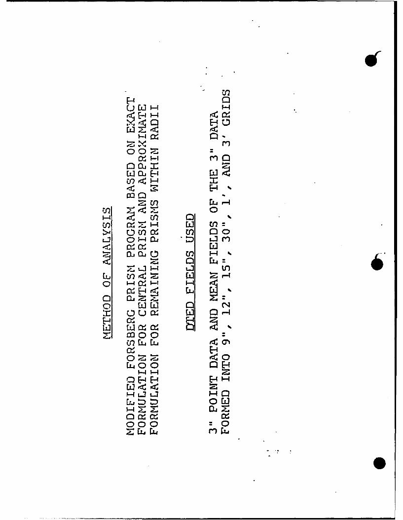
b. Method of Analysis

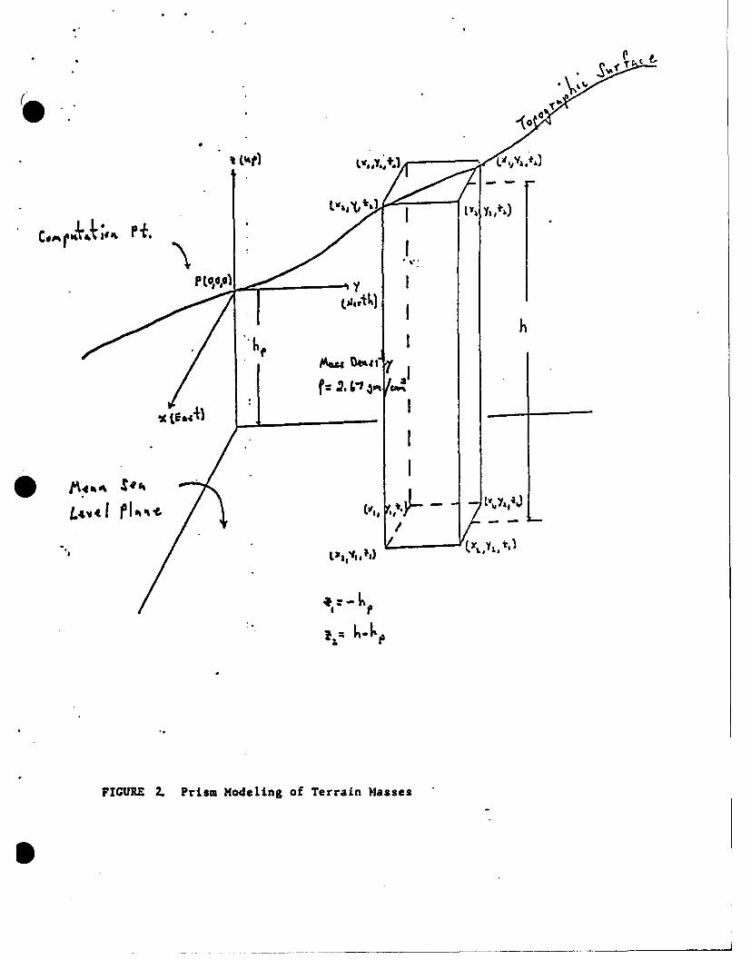
A modified version of the Rene Forsberg prism program was run to computethe topographic terrain effects. T!' program is discussed in Reference 1.The right-handed coordinate system was centered at each computation sta-tion with X pointing east, Y pointing north, and Z pointing up. Prismswere formed from the geoid base up to the DTED topography of an assumeddensity of 2.67 gm/cm as illustrated in Figure 2. The integration wasperformed numerically using the distances from station coordinates to theeight corners of each prism. The surface station height was offset 1 cmto avoid the central prism from being automatically eliminated from theprogram and to avoid the station from being located within the centralprism boundaries.

c. DTED Fields Used

A 3" point DTED field was built around the stations from the same datathat DMAAC sent to Bell Aerospace/Textron. Also created were 9", 12",15", 30", 1' and 3' mean fields from the 3" point data. When usingboth an inner field and an outer field around a station, the prisms mustproperly fit together. If the inner field is the 3" DTED, then the outermean field must be a multiple of 6" for the prisms to fit together.

d. Formulation

Terrain mass modeling is accomplished with homogeneous rectangular prismsin the calculations. Gravitational formulas for such prisms are knownfrom MacMillan's work on potential theory in Reference 2. The prismdimensions for this study were controlled by the description of the topo-graphy. Figure 3 shows the indefinite integral solutions that are usedto compute exact values for ten gravimetric quantities at the computationpoint P in Figure 2 for a single prism. When the separation between aprism and the computation point permits, approximate prism formulationsare used instead of the exact ones. Figure 4 gives details on how aseries expansion for a. prism's potential may be derived by formulatingthe reciprocal distance "r" as an infinite series in terms of the Legendrepolynomials. Using only the first few terms of the potential series, alldesired gravity quantities may be found hv simple differentiation. Theexact formulation is normally used for the central prism while approximateformulation is used for all remaining prisms to obtain the desired gravityquantities.

I1. RESULTS

a. Tabular Output

Tables I and 2 show the effects of topgraphic modeling by different DTEDfields within a 12' radius about the two surface stations. The variousterrain fields used were 3", 9", 12", 15", 30", 1', and 3' DTED. Thesame investigation is repeated in Tables 3 and 4 for the computation

2

points at elevation 5000 feet above the geoid and directly overhead theground stations. Terrain effect variations due to unit step increasesover the interval, 6' to 13', in the radius of a central zone of 3" pointDTED are shown in Tables 5 and 6 for the ground level stations. In theremaining tables, terrain effects are'accounted for by employing the 3"point DTED in an inner zone and one of the mean DTED fields in an outerzone. It waw discovered that the prism program requires the outer gridfield to be a multiple of 6" for the prisms to properly fit together.This is the same as saying that if one extends the 3" field, then theouter mean field grid points must coincide with a 3" point. Examples ofouter fields would then be 12", 30", 1', and 3'.

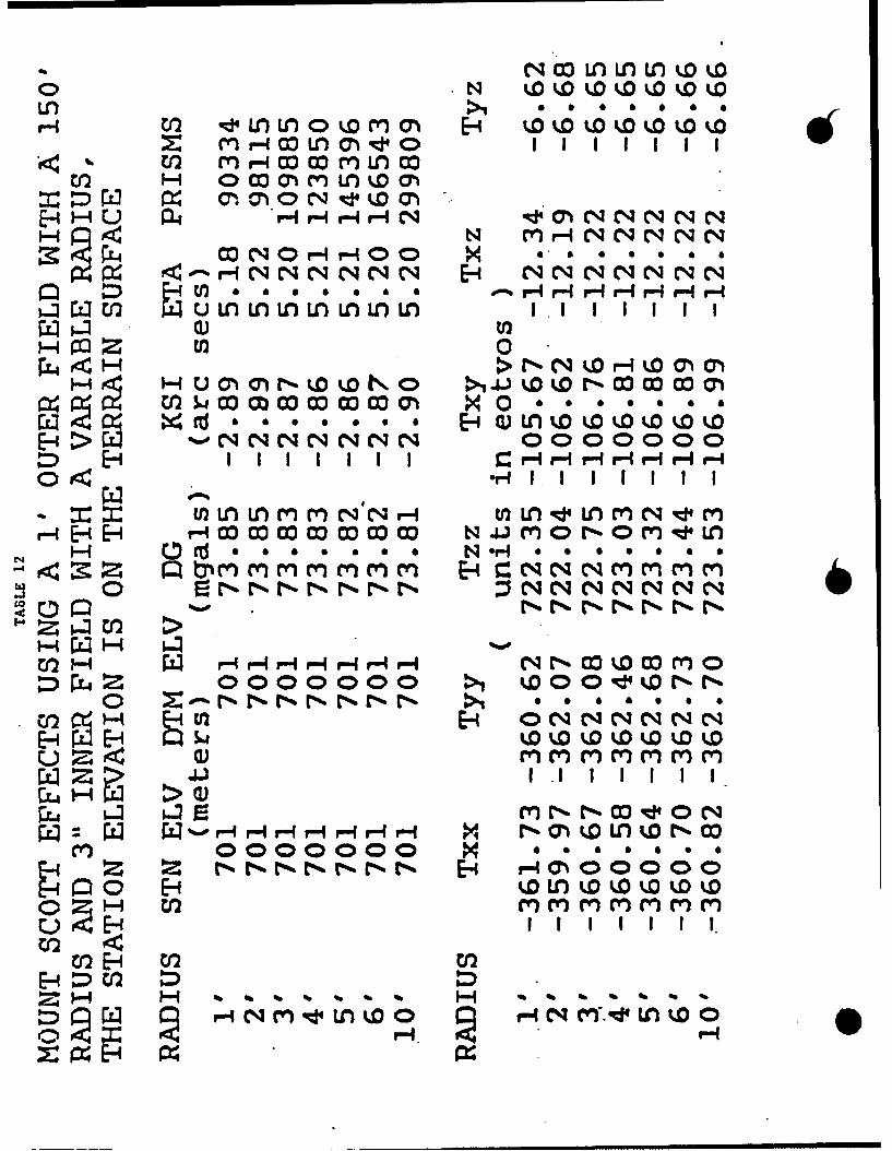
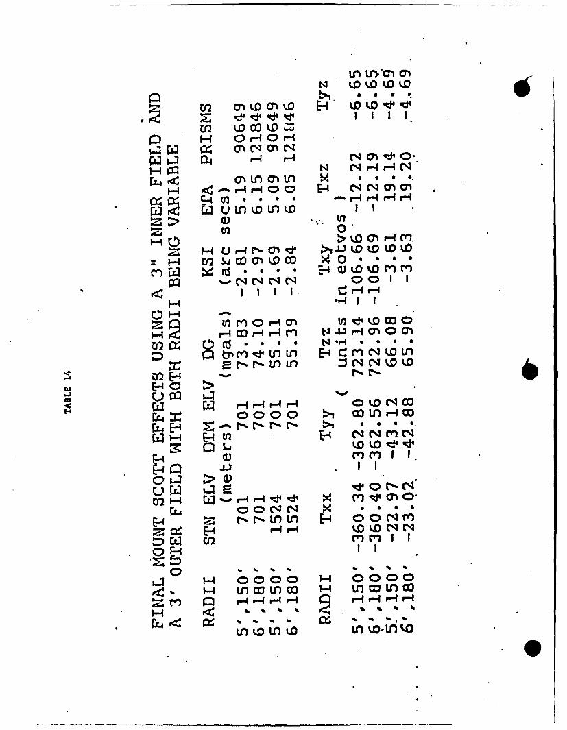
Tables 7 and 8 indicate variation in terrain effects caused by mean DTEDrepresentations in an outer zone of radius 30' and an inner zone radiusof 12'. The means considered for the outer zone terrain modeling were12", 30", 1' and 3' OTED. Each table displays results for one of thesurface points, Sunset Peak or Mount Scott, and the related overheadpoint. Tables 9 and 10 reflect the usage of 1'omean DTED in two expandedouter zones, one of radius 20 and the other 2.5 with an inner zone radiusof 12'. These are again composite tables for a pair of ground/aloftstations. For the ground level stations, Tables 11 and 12 indicate ter-rain variations due to inner zone modeling with different radial extentsover the interval ' to 10' while the outer 1' DTED zone was extended outto a radius of 2.5 . Tables 13 and 14 are composite tables for a pairof ground/aloft stations where the terrain modeling was accomplished byan inner region of 3" point DTED and an outer zone of 3' mean DTED. Theradii of the inner and 8uter regions were 5' and 2.50, respectively, inone case while 6' and 3 in another.

b. Analysis

From Tables 1-4 the pronounced decline in the ground elevation at MountScott with the increasingly smoother DTED modeling in a 12' central zoneindicates steeper terrain here than near Sunset Peak. A 200 meter changein elevation occurred when the 1' DTED field was used instead of the best3" point DTED representation. Tables 1 and 2 clearly show the need forthe best DTED modeling in the immediate vicinity of each ground stationas large gradient variations resulted even with the g" mean DTED field.The same requirement applies to the aloft stations even though the vari-ations are not as striking due to attenuation effects with altitude.Tables 5-6 show diminishing contributions from successive additions of 1'bandwidths of 3" point DTED to a central zone with an initial radius of6. The aggregate contribution of the seven 1' bands is between -23 Eand -25 E on Tzz and 11-13 E on Txx and Tyy. These tables also show thatthe off-diagonal gradients experienced magnitude changes of less than 1 E.

Later tables will indicate an improbable need for continuance of bestterrain modeling beyond the 6' radius. From Tables 7-8 the inclusion ofan outer band, extending from 12' to 30', has an impact of approximately-12 E on Tzz, 5-7 E on Txx and Tyy, and between -0.02-E and 0.7 E on theoff-diagonal gradients irrespective of terrain modeling by 12", 30", 1'.or 3' mean DTED. This beckons the use of either the I' or 3' mean DTEDfield for outer zone modeling. Tables 9 and 10 show that outer zone

modeling with the ' mean DTEU field must extend to 2.50 for the diagonalgradients to exhibit satisfactory convergence. For all cases, the span of1' mean DTED from 30' to 2.50 contributes between -6 E and -7 E to Tzzwith approximetely -0.5 E of that i'.dng from the band 20-2.50. This samehalf-degree width band accounts for less than 0.4 E to the Txx and Tyyvalues. Even 1sss contribution to the results would be expected from anyband beyond 2.5 due to the nature of the kernel functions. With entriesin Tables 9-10 as benchmarks, results in Tables 11-12 show that the innergrid radius for the 3" point DTED may be reduced to at least 5' or 6' fora 2.50 outer radius with the gradient changes being 0.24 E or less inabsolute value. Comparing Tables 13-14 with Tables 11-12 shows that outerzone modeling, from 5' to 2.50 with 3' mean DTED instead of 1' mean DTED,causes gradient changes with magnitudes no greater than 0.41 E. Selectionof the larger mean field would reduce computer processing time in thatfewer prisms are needed. It should be noted that each table contains re-sults for the gravity disturbance and deflection of the vertical componentsthat the reader may examine. The deflection components were more affectedby distant topographic masses than the radial gravity disturbance.

When an outer grid is used, the inner grid values are extended furtherthan they were in Tables I through 4. For instance when the 3' field wasthe outer grid and the inner radius was 5' as in Table 13, the portion offine grid used in computations agrees with that of the 8' radius of Table5. Another example is when the I' field was the outer grid and the innerradius was 6' as in Table 11. This agrees with the portion of fine gridused in computations for the 7' radius of Table 5. The inner field isthen extended by one unit of the outer grid spacing to form prisms thatfit next to the prisms from the outer field. This explains why the outergrid must be a multiple of 6" for the prisms to fit together. This alsoexplains the increase in number of prisms for Tables 7 and 8. The 3"field was extended further out by I' and 3' which caused an increase innumber of prisms. However, as one increases the outer radius to 3 , adecrease in number of prisms would be seen by using a 3' outer mean fieldrather than an outer field of higher density. Computer time is thusreduced by using the 3' outer field.

IV. CONCLUSIONS AND FUTURE CONSIDERATIONS

The inner field must be the 3" point DTEO with an inner radius of at least5'.0 The outer field may be 3' mean OTED with an outer radius of at least?.5 . If the field is big enough it would be advisable to use an outerradius of 30 and an inner radius of 6' in general. This would allowconvergence of the topographic terrain effects within acceptable limits.The 3" inner grid contributes the major portions of the qradient valueswhich means that the 3" elevations near the station coordinates must beas accurate as possible. An inner grid that is a less dense mean fieldwould not yield the proper elevations near the station. The outer gridmay be thought of as fine-tuning the values until convergence is achievedwithin acceptable limits. The 3" OTED tapes are written in 3' blockswhich makes it convenient to form 3' mean OTED fields for the outer grid.

4

( One must consider the computer time saved by using 3' mean TED fieldsfor the outer grid as large numbers of stations are computed. The numberof prisms is cut down without sacrificing accuracy. About 90 seconda ofCPU time is added per station with 3' mean OTED out to a radius of 3 and3" point DTED out to a radius of 6'. The radial gravity disturbance andsecond-order gradients converged within desired limits. The deflectioncomponents will not converge as the outer grid radial extent is increased.Conversion of the deflections into the other two disturbance componentsdoes not give near the magnitude of the radial disturbance. We see thehigh frequency nature of the second-order gradients by their rapid con-vergence. The much lower frequency nature of the deflection componentswill not allow convergence in the computation of the terrain effects.

In the future it would be desirable to augment the analysis with morestations in the Wichita mountains. The spectral characteristics andcovariance funcions for both local topography and terrain effects shouldbe defined. Terrain effect computation by the FFT method may be investi-gated in the future for reduction of computer processing time. Comparisonsof GGSS gradiometry data against gradients derived from DTED fields willneed to be made. It would be desirable to incorporate error propagationinto the topographic terrain effects programs as errors in the OTED anddensity assumption become better defined. A major goal is to be able toadd long and intermediate wavelength information to terrain effects forprediction of more accurate gravimetric quantities.

S

p

REFERENCES

1. Forsberg, Rene: A Study of Terrain Reductions, Density Anomalies andGeophysical Inversion Method-s in Gravity HFel-d odelliinq: OSU Report No. 355,April , 1984

2. MacMillan, William Duncan. The Theory of Potential-. Dover Publications,Inc., New York, New York: 1958

00

0

00

C) 0 0

U).4El

Erl 0

LLO LM

I-4rZ:

C UdW e, 0

V-D 0 LJ E-40 EL

co L- U E-4

-4U' 0 <

0 41 -

ELI =10 Lz>~ [-4

V A

Smntse+ ..A 3140 44'NJ 7s9'0 w

1Aour+ Scot+: 34 *4'$ 9903).

L2Jj;.~wto 4 6'I-T tt7Et 4 /Its, 'Liwow I 1F .. 1

**~ ig 'T=

on~. sd,,L ~ I ~ 'i;

NIA CmE oauh I -SA M AI

WJ~±I MO~fAJJS~" ~ -~-+

- *%..L -b .410 I r JoID7'.4: -A

-f S. .4 FMO~~ F ~.P4~cA- -wLI

AL4A 2 A.

11% 441 -- --~ % 5

I. L I\ (r.4; i

jz;k:Fd _ -1 F a

I ~~ 1" a 1-INL loti t

- "7 \Iall K2"__II~~ III 5

UV Sri~

-gA ,

L PY1 rao oorphcTranAayi -WciaHutJi

Ukl-4

I-4-4

m c

:g: E-4

1-4 Ek1 4 :ia; Otrio M

U j M1I. (n 1-m

b.... D 'D~O U I-

E-4 W.Zr

o o 0

o WIl P E-4

t-3 LJ

0L00 CIH

( O09

40tle

FIGURE 2. Prism Modeling of Terrain Masses

I' etT'h e&iul'. THE 7,d~rPI-lTF r&ATEf.A.%L

61AVITY Qu4J~rml AMCQ FguJClIONAL V'rlgAGf~iUMJ

T ) -r

73 itf ii)ti, i )

16L' -l Li4r -j (I )W 1;,

T2 r

is. l T I LEr

Bit[ 7

7-ry9

FIGUR.E 3. ExaCt Prism Formulation for Differnt Cravimeric Qumniies

7= AY

JLZ. A*

POTENTIAL: .Tti/f JI J(;

L&ADJ 71 THE IV1AIR* AfFr%1Xg1iArTV9

~AX%- y At) 1 j LAyA)~+.t~3~7A)''

U~ +1

FIGURE 4. Approximative Prism Formulation of Potential T

44

w0

dL4

C3C44

o C

E-4 E-m 00

0 >

0- 03 *- N -411

O 0 CqC1 m 0 N ON N 0N C) rOCL, r~4 >1 a * * S, 0

E-4 r-IOOOOcO0

O0L U4 ' Vi * * * * *

rU I'* I* r* I) I M ,~ C(-4 H r-4 t-O0 OO

O~ '-4~ IE-

cl :4 40 * 11. do Id *'

v tJ - I r-4 -4 r4 r- r4

rnr4r4IeI ELIvu e-Ia)-4 Nm *E-4 0 * 0 4 *

E-Ha N 4 ~Ln m c4oin~~14' r- r- *l r- N r-

0 E-4 N~. Ajqp0nw r- -t- r - I 0 0 6 0

Wr4f CWN N -4ur--C--

cot cca o)aoa0O rq r-4JU'I W qd4 0O

> r- r-M -

Mfv tz.r-0: n .

030 o0 : : S* 0C)0 0L

LQ ritncId, 1n

(Y) 0 N~~r~ C Nchr--4 Ln WC- (1Cr- N w.Or- rl r- r-4 C'i

C-4 E-4 o r- Ln r c~

0 rJ4 E-4 rtn * * * .

T. nJ N _IPLf)l 0 0r-4

C0 0000 0

tI 1l r- )r o 3'OLn oL cJn

1-4 ~ ~ ~ S Ol *n M C* w C)r4I *

-r4

o 1 w0 Lo r'i' 02 M44 co I e

N -r4 * * * * o*

Ca OU 0 -c oc

COE- r-I. qSd qS: r-40

r a; rC U( 4 C;

LUjL.] L3 5 oir0O

pp 0 p

r-4 r-4 M 010 -4F-4 In wI I I

M) mOn a) a) fn

r-4- on 0 cJ)k 03D4 K 000 0 0 r-

0 0 0 0 0 .

Mfl EdI1 111 N- N wJ~

#4 = u le I I I I I

r- 4 - r4 r4 0

z>X 0 0 9 * 0 *

1-4 o co 00 CC (n

(t.1E- - - ( C;OO O O ' 4

Z LLA 1L L tlLn L n t c - NC~

0 N -L) co *) 0a w

-3 >

oo a) coLflr400f0

LI mi~ Lrr-4 r4

p... >W>II

ILI > r-4-4l 1-l O H r H lf-4

cu~ U Lj >L

luLi r

0 03 ON r4W.

-4 d r : r-4 N~ ~m m0ce N w d

E- d-r4 C, U N m

1-4-E W -r4 r4H4M

n ,t *f X * * * 4eel u r-4 r-4 W

w a N0 mN 0 Mt.0 a

1-4 d. m -Q4

L2H -t;4-n % or-

0 NDOw ll mqdl N

cOOO 4Vn

HO LO M4~r -d *- N *

r-44 0( a)0

> Ln- -d -Q N

-4 -qd -d -d -,Z -q

EL]N NaiN a3 0L 40 r4 M t.0

E- L u)LnLnL) n mwLnm

IN-

1:4 ~ ~~ ~ ~ ~ r- Ir N m N m N -4 -4 -I r- r- -I I -

E- r-4 E-4 r-4 *- *- r- P- H

:r. N- c ima0 -t

*p . .. . . .

E-4- r,4 cNN C C 4

r- 4r- r-- rIr-4 r-l r- 0

IN 0 0 . 9 * a * 00 r- rO-4 r- IHr- r

N rl rn m re) M mrElLn nLo InLn Ln L InflO -jN Mt* qJ4I

0N i- * e .-r 0) a) t4 a4 %

0o u >C k dO 04E j (N r-4 r-44

H- Lrir

,c~E-4 P Q* -'. * f* *

U 4 ) U) - )r- DU ,4r

EL u N r- -- r-4rH4r-4 4

44I

m~~ ~ r- N mQ0 0 Q0 to

i- nL * n o ci~o

C) t 4u

u r-4 r- r-4 - r 4 r4r4r- --l" -iZ r Q)I I I I I I I I

H -0 000 0 liL tlqo t w t w

r- I Ir I I I I I 0 0 0 0 004 mH m 0 m - N1.

oH P 0bpCOr- - -q - N o-4 0 0 0 a a 00

I- m0 m> 4 4

r-I2 W- ~~r 4r -rr-l r-q

7jI- a-tf a a a 0 0 0 0

P~ &Jri0 td -

0: 0trr 0 0 0 0 0 M 0- DMC d

H) p) INa r r;c%

Por-co0d -4 N m - l- c n0rlN

1-4 P-4P-4 r-fr-ri H-

* M Cf) o0rrC o r- r-

00 rN. Q0 *N C> r- t

0 0 Lz 0 0 0 0 0 0 0 00MCY C l4

Q) I I I I I

E_ -4 u -r-Na

N) r4 N C1 '- N-4 - r- E- r- r- fn enB

* . 6 r4-

) L-3W r-) r-) m m m mm00-

In >1 S B ......

LU)

E-4 ~ r-4 r- r- H r-4 -4 -1ii t l

0c L r'4-4 re) 4 r-4C M -W - ~ -

* < -4 r- y - Y

utpL

r-1 r)"1crIooE' m F-Imm I II I1I11I1c o 4 N o -r * . - W

CL nm m. rm mm )4WLMr4NC%

4 -4 . 4,q X - M C -4r-or4 -oc E- 4 N N C,-4 r-4 *- r- r4 NCN N C a 4

C) E-4 M - 6 a - a r-Il I P- I - FIr- -

tl)

zrz II -,t 1 r-r- r- w

-4 1-4 U f0o mC4CluI

m-~ m 1 % )U)0c h0 O%

tfq E-4n r4rfr- - r4w mcoa -000000 r-'

D4 > LJ Hr-4 r4w

H~w -- m-- H 0~'~r0~~~ III- M14r4 -

44I

N~~ E- r- 4000

r-r- co r-- a)~W

U)~ a) 0lU) Lna n0

10 ~LOOaO0

0H 0. to r N x a a a

W4, kO M 'd S nL

~~L-~ N-Lf. r-4 Nla) U)

- U) ..0

r> U)% >~Lnj)u L nL

-1-4 tlO~~

E-44r

Er 4 I > -0 R4 NJ)rIto0

5) uz ) mn n r r- r

rnJ -'-e3noq

>0

aHL. L() t Ir

Y'- 1400 00 - 0000 a1-4 q~4 :d4. IJ I-I r- -4C

r- -4 r-4 r-4f4 r- - -

11 10mN W 9.0r-- N

N 0 0.

H U) ~ ~o'dom il

<tD r~I-4 J--4 C 0 a)0

r4 LnC a) C a04 M iM M mecq D0

N (CH Hr-o0r*_o x 0N~ N r--4 H c~~cn o

tn af 0 0 0 - 4H r-r-u- -cil m Jp I Icu LI,Lfl .0

H ~-umoowo ta4j C 0 ccz U L, C t.Q0Dr* XO, 0 0 a

H n r1%-110 tn0 r4

r~j r-4 Ul co 0 N ji0 LflO) dr0 t 6 & N 9H 0 0 0

Ca~r-I r-4 r-4 a 0)CN000 rl -

ma Htn H c rm m

1LZ4 >

r- r- r Lru Ln H r- Hrlrn

u In

~~~oc -- 0 0-4 0000

*0v4 r- H -,4r-4 H-lHH-

0N w Nr ! r r

II 0 14 O~ 00 0) -I n V CI

E-4 rN- Ln Ln LnA Ln LA L1- Q 04 NN NN

wrj u N N NN r r

~> OWN R;:PNM ***

E-4 >-4000000m0mm r

1- C rd a & 4 * * 0 N4 * * 6 0

Z ,L L nL LAU L H E4w 1. W D

4 c.yC( r)Mf )Mr)> ,od

E-1,

uu

B_ 5 o0 n 0) 0) r

A-as2 e d d d 4 E4 -;r;r. _

:Z4 I-'

cE-4

E-Si) C

loN

E-1W- f rI V- qN 0NCvCA -H- N m INN 4NC4

co N 0 ,-Ir4 00 x a 5 0000a

F-i cq N N * 4 * % N E- *

POZ 0

triLn Ln m m NNr-iP P r-Ew wwEw- N jM 0 r*- 0oMjd M

1-4 Ord a * * * a 0 * N*- OH *

0 Q~rCrN~

m M4 -4 r- H r4r-4H-4 4

0 0000000

U) r-4 E-42

~z~'r-I r- -- 4 r- r-

C'~~r- 00000 0 0 00eS

Ho

1-4'

024 C-4 oLhE-4 t-4 a) oS '0 w2 clo w coi

E- u7 d0r4

W- u-

:2; >(1)tO oX

- 4 >c

m - 0.- 02.Jfrm %O * o

H - 0 mm t

$ nLn d ,p Na-4 r: w *-.nd9 LO ) Ln L

hiJE-4 0 > I

CO m o m W* *E-4 *-%fdo 41:4 (qp c:to

P n teLo,

-i Xa 5 ld

E- co~~ N - ~ 0w20 Enirf-

07 =0%

H- 0000 H0000: a H r -, n ~ 1 4 I f~ ~1-4 - - 4

1% *Al

0nwL

Ln ut.*O aN W W W~f~f

:> lilt.

H o0O

H ~ H- C4 4Oc .

M 0

0

PQ q (4 Ncq001 1

E-4i 0 >-H- r-40 I ll c

44 a)U- -4C

'-4~r- 000 t', tL l

N cqH rt~flf 0 or

1- m w mi

H bLCn to tnL nD n%

0 P0 -

H- 04 H0HOM 0

4ze H omE-4 0 0 Z:) ED

04 H w c

E-4 E 1 m w 0o -H r4 Ho

o aN oN

:D 0 4U H Z QH4 HO H

0 m 0 z0 H0 H HZ r4 rr

ml m 0 r" -x HE-4 Ez3 -4 (n tON0

H- Nr U

0., W . ,Hr2 O z i-iN• . 00

0.4 z- 0ON) z 0 p

coCf)

ELI EL*- tfl 0 >

Eli 44Euo U U4OE~~iEr] u Uct f~4E~

t fC u i L i~F ~ C

H ~ ~ -H i~ -E-4 Z~L :a;Cr ruDi- E- &E-

r, Li i 1-41- )

-~ uN :>4 c-u-IH

;- )E-

u z -4 H :H= -Ci~( Li Hi PiU ~ ~

~~L C)0 I4 00 E-w0~~~~ Eu00 OH Uv0

~5 ~z H u H qH CEd C i L i id EI ?6- -to tt t

H~~~D H H oH O"4- ~ - ~ -

>4

z0 00 E-H H. >4

H H - 0P

0 H ( . HH

H HO x E-

H 44p4 Hx

HZ >4E- H

u mH

H~~fw m, zU2>40

0H H oz z 04 44-40 H-Hi 0tH 4

>4 0 ~H 0= H

X E-4HZ W W C0

mH u H - zo

HHO

H 0 QIZ~

-4 1- HH0 I4

--KK-K-

EFFECT OF TERRAIN REPRESENTATION, GRID SPACING,

AND FLIGHT ALTITUDE ON TOPOGRAPHIC CORRECTIONS

FOR AIRBORNE GRADIOMETRY

by

Klaus-Peter hchwarzMichael G. Sideris

I.N. Tziavos

The University of Calgary2500 University Drive N.W.

Calgary, Alberta

CANADA T2N 1N4

ABSTRACr

The fast Fourier transform (FFT) algorithm is used to efficiently compute

terrain corrections for airborne gravity gradients. The formulation of the

equations is given in detail, deriving the spectra of the gradient components

of the gravitational tensor directly from the spectrum of the gravitational

potential. The terrain is represented by either line masses or by prisms.

* Results of the method are given for a very rough digital terrain field in the

Kananaskis area. Comparisons of the terrain corrections in common points for

grid spacings of 0.1, 0.2, 0.3, 0.4, 0.5 and I km are made using the line mass

and prism representation of the terrain, for two different flight altitudes.

Results indicate that for a flight height of 1 km above the terrain, a 0.5 km x

0.5 km grid of elevations is adequate for an RMS accuracy of 1 Eotvos, while to

retain this accuracy for a flight height of 0.6 km a grid spacing of about 0.25

km is required.

EFFECT OF TERRAIN

REPRESENTATION, GRID SPACING,AND FLIGHT ALTITUDE ON

TOPOGRAPHIC CORRECTIONS FOR

AIRBORNE GRADIOMETRY

BY

I.N. TZIAVOS*, M.G. SIDERIS AND K.P. SCHWARZS

THE UNIVERSITY OF CALGARY

DEPARTMENT OF SURVEYING ENGINEERING

CALGARY, ALBERTA, CANADA

On leave from

THE UNIVERSITY OF THESSALONIKI

DEPARTMENT OF GEODESY AND SURVEYING

THESSALONIKI, GREECE

Presented at "The 15th Gravity Gradiometer Conference ", Colorado Springs, Feb. 11-13, 1987

NEED FOR ACCURATE TERRAIN CORRECTIONS

MAIN SOURCES OF NOISE (instrument independent)

- Topographical noiseDue to surface topographyCan be minimized using DEMs and DTMs

- Geological noiseDue to density variations in the upper crustAdditional information needed for its estimation

- High frequency effects "filtered out by flight altitude

REQUIRED TERRAIN CORRECTION ACCURACY

- 1 E RMS or better at flight altitude

- Depends onTerrain sampling rate (grid spacing)Terrain representation (prisms or point heights)Flight altitude(Extent and topographic features of the area)

FFT EVALUATION MOST CONVENIENT

- Fastest approach for large data files

- Availability of DEMs

- Homogeneous coverage in results e- Specral analysis and interpretation

OBJECTIVES

DERIVATION OF CONVENIENT COMPUTATIONAL FORMULAS

- 2D convolution integralsFast evaluation using 2D FFT routines

- Relationship between spectra of prisms and point heights

ESTIMATE THE EFFECT OF GRID SPACING

- 0.1km x 0.1kn grid results used as control values

- 0.2km, 0.3km, ... , i km grid results compared to those of 0.1ikmgrid for 1.1 km flight altitude (zf = 1.1km)

ESTIMATE THE EFFECT OF TERRAIN REPRESENTATION

- Prism representation results versus point height results

- Comparison for a grid spacing of 1kn and zf = 1.1km

ESTIMATE THE EFFECT OF FLIGHT ALTITUDE

- zf = 1.1kn and zf =0.6km were used

- Comparison for various grid spacings

PROPOSE THE GRID SPACING AND TERRAIN REPRESENT-ATION NECESSARY FOR A 1E OR BETTER RMS ACCURACY

*AT FLIGHT LEVEL

COMPUTATIONAL FORMULAS- .Z flight

. levelzI

Zf

y P(iptypthp) zo =consL.

Za -hp X sea0 ---hlevel

POTENTIAL OF TOPOGRAPHY AT Po

0 dx dy dz

V(xp,ypz o ) = Gp I . , S2 =(X-Xp)2 +(y-yp)2 (1)

E h [ s2 + (-zo) 2 112

GRAVITY TERRAIN CORRECTION AT P0

5V(Xp,ypZo) h z- zo

t(Xp,ypZo) =- = Gp If dx dy (2)OZo E 0 [s2 + (Z-zo)213/2

Series expansion of (2) around Zav, neglecting orgers higherthan 2nd , gives in convolution form

t(xp,ypzo) =. 2xPZav

+ Gp[hl(xpyp)*kl(xp,yp)+h2(xpyp)*k2(xpyp)] (3) 1*

(= Bouguer affect + effect of residual topography)

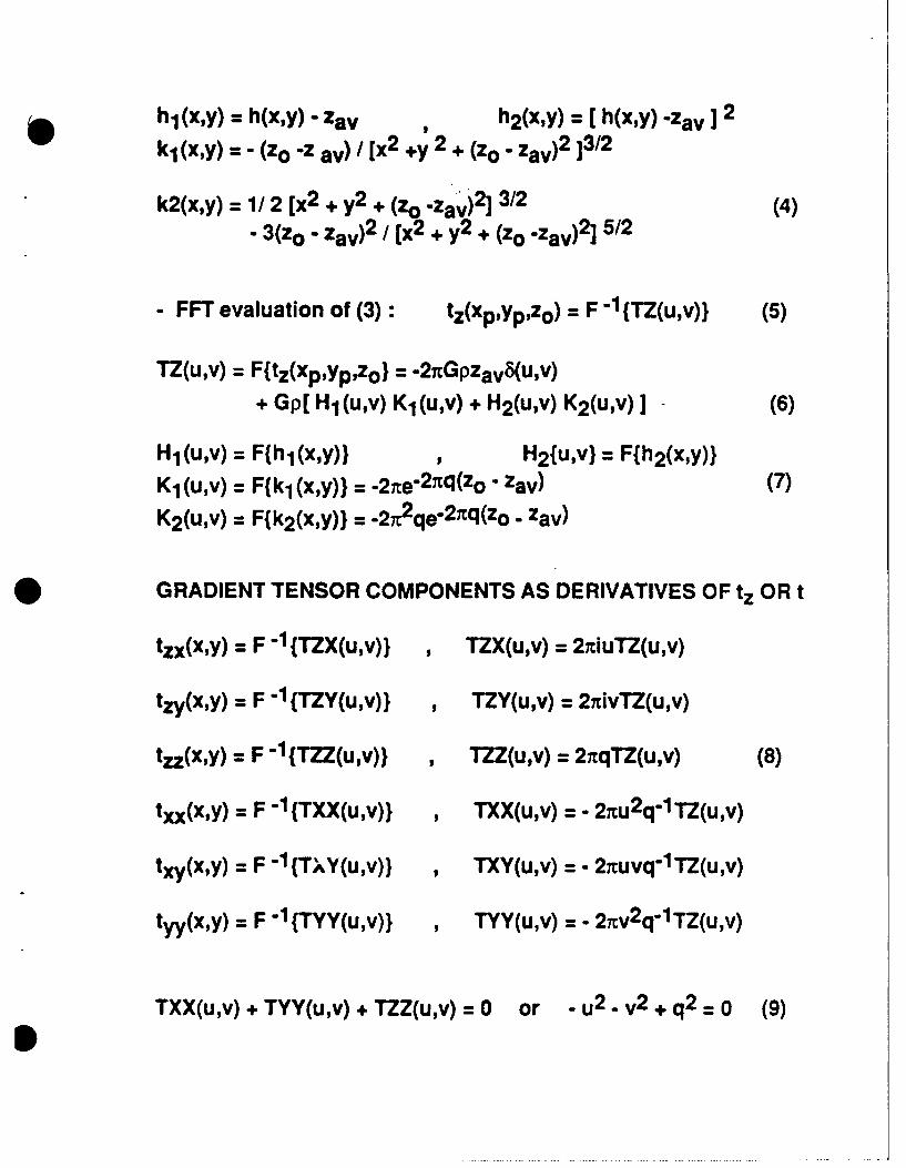
h h1(x,y) = h(x,y) - zav h2(xgY) = h(xgy) -zav ]2

k, (x,y) = - (zo -z av) / [x2 +y 2 + (z0 - zav )2 ]3/2

k2(x,y) = 1/ 2 [x2 + y2+ (zo zqv)2] 3/2 (4)- 3(zo - zav)2 [ x2 + y2+ (zo -zav)2] 5/2

-FFT evaluation of (3): tz(xpgypgzo) = F -1{(TZ(u,v)) (5)

TZ(Li,v) =F~tz(xpgYpizo} -2iGPzavS(ugv)+ Gp[ H1(u,v) Kl(u,v) +H2(u,v) K2(u,v) J (6)

Hl(u,v) =F{hl(xy)l H2{u,v} = F~h2(x~y)}Kj (u v) =F~kj (x y)) = -,.ne- 27rq(zo - zav) (7)K2(u,v) =Fjk2(xqy)} = -2i2qe2nq(zo - zav)

* GRADIENT TENSOR COMPONENTS AS DERIVATIVES OF tz OR t

tzx(xgy) = F 1{TZX(uv)) 9 TZX(uv) =21ciuTZ(u,v)

tz(xoy) = F -1 TZV(u v)) TZY(u,v) =21c~vTZ(u,v)

tz(xoy) = F '{TZZ(u v)) ,TZZ(u,v) =21cqTZ(u,v) (8)

txx(xgy) = F -1{TXX(u,v)) , TXX(u,v) = - 2iru2q-lTZ(u,v)

txy(x,Y) = F -1{TAhY(u,v)) 9 TXY(u,v) = - 27ruvq-ITZ(u,v)

ty~xy)= F -1{TYY(u,v)} , TYY(u,v) = - 2irv2q-lTZ(u,v)

TXX(u,v) + TYY(u,v) + TZZ(u,v) = 0 or -u2

-v2 + q2 =0 (9)

20 PLOT OF THE TEST AREA Urnm x 1km DM

~'coo

1j?7-C P

-01

- }y -

- ~ x -

SSTATISTICAL ANALYSIS OF TOPOGRAPHY AND TERRAIN

CORRECTIONS IN THE 36 krni x 56 km TEST AREA OF ROUGHTOPOGRAPHY USING A 0.1km x 0.1km GRID OF POINT HEIGHTS

Topo- Ag corr. Corr. for tij at zo =4.5 km (zF = 1.1km)Stati- .. . ... -

grphy z=hp z=zo txx txy ta -tyy tyz tzsticsmeters rga Eotvos

min 1378.0 -313.1 46.6 -76.7 -40.7 -74.9 -45.9 -62.8 -129.7

max 3413.0 -141.0 14.6 72.0 38.9 82.4 70.5 69.2 86.5

mean 2129.6 -226.7 -15.1 0.0 0.3 4.6 0.8 -3.5 -0.8

s. d. 350.2 37.3 12.2 35.7 14.6 37.2 18.5 23.9 45.5

RMS 2158.2 229.7 19.4 35.7 14.6 37.5 18.5 24.1 45.5

EFFECT OF GRID SPACING(USING POItT HEIGHTS AND zf = 1.1km)

RMSdifferences " ZZ

[E] .. Izx

.txx

3- si2 Y-

0 LI_.M grid spacing

0.1 0.5 1.0 [k i]

-z-components more sensitive than the horizontal

a Effect on the horizontal components dependent on the terrainfrequency content along the x and y-direction

a 1 km grid insufficient for < 1 E RMS accuracy

- 0.5km grid sufficient for c 1E RMS accuracy

- 0.25km - 0.35km grid spacing necessary for < 0.5 E RMSaccuracy

- Bias always < 1E for 1 km grid< 0.35 E for 0.5 km grid

* EFFECT OF TERRAIN REPRESENTATION(FOR zf = 1,1km)

DIFFERENCES BETWEEN THE RESULTS FROM PRISMS AND FROMPOINT HEIGHTS AT FOR A 1km x 1km GRID

Terrain correction differences, in E, for tij at zf = 1.1km

Statistics txx txy txz tyy tyz tzz

min -6.2 -1.5 -7.0 -1.6 -2.1 -7.3max 6.5 1.1 8.1 1.5 1.6 6.5mean 0.4 0.0 0.5 0.0 0.0 -0.4s. d. 3.5 0.4 3.5 0.5 0.6 3.6RMS 3.5 0.4 3.5 0.5 0.6 3.6

- If TZ(u,v) is the spectrum of tz(xy) computed from prismsand TZ(uv) is the spectrum computed from point heights,then

sin(ur Ax) sin(vtAy)TZ(uv) TZ(u,v) (10)

unAx VICAy

- Prism representation has smoothing effect on high frequencies

- x-components more affected than the y-components becausethis particular terrain has more high frequency content in the x-direction

- Differences of up to a few E are to be expected in the more

densitive components

tEFFECT OF FLIGHT ALTITUDE

(U3!NG POINT HEIGHTS)

RMSvalue[E]70

60 tzz

s - tzx

40

30 .ty20 .........- * - * - tyy

10-

0 'grid spacing

high values : zf =0.6km (zo=4km) ;low values : zf =1.1 km(zo=4.5km)

a Attenuation stronger for z-components

- x-components attenuated more than y-components due tounisotropic terrain frequency distribution

- Attenuation Independent of of grid spacing

- Accuracy of results dependent on grid spacing / altitude ratio0.25km grid to be used with zf = 0.6kn above very roughterrain for < 0.5 E RMS accuracy

CONCLUSIONS

TERRAIN CORRECTIONS NEEDED TO CORRECT FOR THE" TOPOGRAPHIC NOISE" ON THE MEASURED GRADIENTS

REQUIRED ACCURACY AT FLIGHT LEVEL : 0.5 E - 1E

- Depends onGrid spacingTerrain representationFlight altitude

- Effects on horizontal components depend on terrainfrequency content along the x and y-direction

GRID SPACING

- Affects more the z-components

- Accuracy decreases with increase of grid spacing

TERRAIN REPRESENTATION

- Point and prism results can differ by a few E RMS

- Prism representation is more accurate

FLIGHT ALTITUDE

- Stronger attenuation for z-components

- Attenuation effect rather insensitive to grid spacing

.

RECOMMENDATIONS

FFT TECHNIQUES RECOMMENDED FOR THE COMPUTATIONS

- Convenient formula derivations in the specral domain

- Speed, easy handling of large data sets

- Homogeneous coverage

- Frequency domain analysis and interpretation of data andresults

FOR zf = 1.1km AND zf = 0.6km, 0.5 km AND 0.25 km GRIDSPACINGS RESPECTIVELY ARE NECESSARY FOR < 1 ERMS ACCURACY

Ax / zf = 1 / 3 appears to be a good choice

ACCURACY EFFECT OF HIGHER THAN 2nd ORDER TERMSIN THE EQUATIONS TO BE INVESTIGATED

TOPOGRAPHIC EFFECTS IN AIRBORNE GRAVITY GRADIOMETRY

by

Rene Forsberg

Geodaetisk InstitutGamlehave Alle 22

2920 QiarlottenlundDenmark

ABSTRACT

The gravitational signal due to terrain masses will play a dominant role

in airborne gravity gradiometer surveys over mountainous areas. The variations

in the gravity gradient tensor elements may easily attain magnitudes of several

hundred Eotvos units, thus being much larger than typical signals associated

with possible geophysical structures of interest.

To smooth the gradient field and enhance "geological" gravity gradient

anomalies, the gravitational "noise" caused by the topography may be attenuated

'i using available digital terrain models, from which the elements of the terrain -

induced gradient tensor may be computed efficiently at aircraft altitude using

either space domain (integration) or frequency domain (FFT) methods.

In the paper, both of these computation methods are outlined and compared,

and typical magnitudes of the effects are illustrated by examples from the Rocky

Mountains. In general, statistics of the gradient variations may be inferred

rather easily from emperical ACF parameters of the topographic heights, and the

paper concludes with a number of such examples for areas of different types,

from lowlands to high mountains, yielding useful "hand rules" for the gravity

gradient terrain effects in future gravity gradiometer surveys in particular

areas.

p

TOPOGRAPHIC EFFECTS IN AIRBORNE

GRAVITY GRADIOMETRY

Rene Forsberg

Danish Geodetic Institute

whytzrrar~n reutin'

- wPracca comptai u '(;?

or Wr methods)

P sxanteds: Newter nd ColoradoiF.1

Presented at "The 151h GravItY Gradlometer Conference ", Colorado Springs, Feb. 11-13, 19C^7

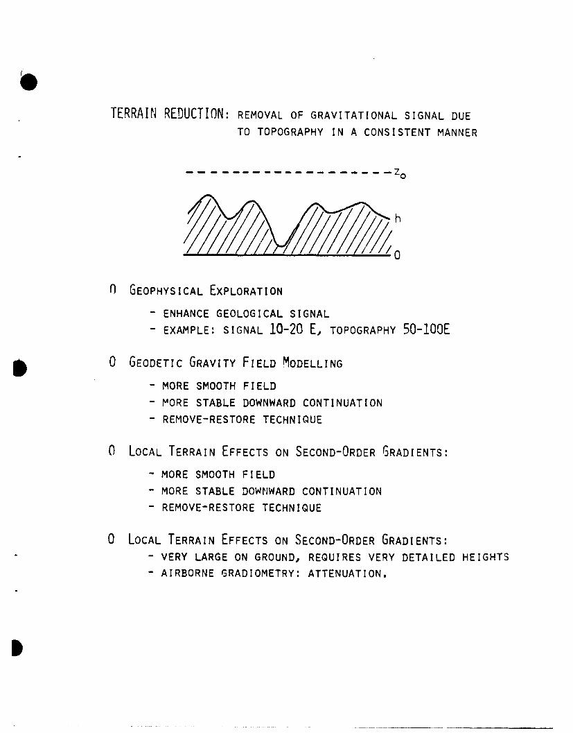
TERRAIN REDUCTION: REMOVAL OF GRAVITATIONAL SIGNAL DUE

TO TOPOGRAPHY IN A CONSISTENT MANNER

h

-- 0

0 GEOPHYSICAL EXPLORATION

- ENHANCE GEOLOGICAL SIGNAL

- EXAMPLE: SIGNAL 10-20 E, TOPOGRAPHY 50-lOOE

0 GEODETIC GRAVITY FIELD MODELLING

- MORE SMOOTH FIELD

- MORE STABLE DOWNWARD CONTINUATION

- REMOVE-RESTORE TECHNIQUE

0 LOCAL TERRAIN EFFECTS ON SECOND-ORDER GRADIENTS:

- MORE SMOOTH FIELD

- MORE STABLE DOWNWARD CONTINUATION

- REMOVE-RESTORE TECHNIQUE

0 LOCAL TERRAIN EFFECTS ON SECOND-ORDER GRADIENTS:- VERY LARGE ON GROUND, REQUIRES VERY DETAILED HEIGHTS

- AIRBORNE GRADIOMETRY: ATTENUATION.

I

0 MODIFICATIONS FOR OPTIMAL GRAVITY FIELD MODELLING

(COLLOCATION ETC.)

- IMPORTANT TO AVOID BIAS IN COMPUTED TERRAIN

EFFECTS, ESPECIALLY FOR COMBINATION SOLUTIONS

WITH TERRESTRIAL GRAVITY AND DEFLECTIONS.

- BIAS OCCUR IN TXX, Tyyj AND TZZ WHEN COMPUTATION

AREA FINITE AND MEAN HEIGHT > n!

- REMEDY: REFER TO MEAN HEIGHT OR USE ISOSTASY!

- BETTER REMEDY: RTM - RESIDUAL TERRAIN MODEL

-Zo

href

0

RTM ADVANTAGES:- HEIGHT DATA NEEDED FOR SMALLER AREA- CONSISTENCY OF NEIGHBOURING SURVEYS

- CONSISTENCY IN PRISM AND FFT METHODS

0

COMPUTATION METHODS: PRISM INTEGRATION AND FFT0

1) PRISM METHOD

NUMERICAL METHOD

z _ _ 1 ? 1 _ ,,C1t 2,

0 x

APPROXIMATE FORMULAS (MCMILLAN): T - fM(" "j4 rf)

TZ, ,+',- ,_. r.,-. ' ,, 7z +24)T ., * - , + , ,L ,-k, . ZT = : , £ -+ j , 2ir a

TMPLEMENTATION: DETAILED/COARSE GRID, INNERZONE SPLINE,

AUTOMATIC FORMULA SELECTION

2) FFT METHOD: PARKER EXPANSION

-Zo

ex h

href

, 0

co = (h-m ,z ,.F -ze (V--Zt4j

F: FOURIER TRANSFORMATION, W = (U+V 2)

GRADIENTS: xx 6lxxT

"I z :-i.,, T

IMPLEMENTATION -Hj H2 ,,,. REAL TRANSFORMS

-COMPLEX FILTER INVERSE TRANSFORM: PAIRWISE

RESULTS

~0

I I

EXAMPLE: W4HITE SANDS, NEW M1EXICO

*33aN - 340N, 1)70W - 10160W, ELEV. 0nm

0,9' x 0,.5' HEIGHT D T:A, 102x102 POINT FFTj 30' RTM

SE

NE

INCREASING FLIGHT ALT'-TUDE: ELEVATION 5Y M.

TZ%

NE

PROFILE TEST: 33.3 0N (PASSING 2680 m PEAK)

C9 -GRADIENTS AT 3000 Ml LEVELLEGEND&

---- TYZT-rYY

07

0 30 s0 90

* ICOEMOt- TZZ

-- TXX

0 0sog

0 30sos

DITAC IK

o .. S FI0 PRIS 90FT z 19, x :14 n

EXAMPLE: CENTRAL COLORADO

390N - 400N, ln7oW - 106011, ELEV, '48Vn m, L.j l % ? C 2 -i

COMPARISON AREA FFT PRISM :30.2 -39,9, 106.8-1%5.2

HE

SE

00

0~

NE

NE

SS

NE

DTM PLOTOverhojnirng: 0.05

39.2 d9 39.8 dg-106 8 dg -106.2 dg

NE

SE

OTM PLT~o opt2Overhojning 0.0539 2 d 398 09

-106.8 ag 036 2 d9

TABLE 1, COMPARISON TEST - 441 POINTS (EoTvos)

Txx Tyy Tzz Txy Txz Tyz

COMPUTED MEAN x -(,6 1.4 -.9 -4. 1.oGRADIENTSRS

o" 36,0 34,5 57.0 20.3 43.2 41,n

RMS DIFFERENCE 0,6 0.5 n,9 n 5 ,n 1,qFFT - PRISM

(N=8)

TABLE 2. DEPENDENCE ON NO. OF FFT EXPANSION TERMSR.M.S. DIFFERENCE TZZ T

N = 1 22.2 8,3N= 3 5.5 1.6N 81,N 15 0.9 0.6

I

COVARIANCE ANALYSIS

0 TOPOGRAPHY ACF - GRAVITY ACU (FIRST ORDER PARKER)

- GRADIENT ACF AT ALTITUDE

0 SELECTED TOPOGRAPHY ACF: SINGLE DIFFERENCE LOGARITHMIC(FORSBERG, 1986)

CONSISTENT GRAVITY ACF - CLOSED FORMULAS BOTH ON GROUND

AND ALOFT, E.G.:

RESULT AT ELEVATION H:

T FIXED -" D FUNCTION OF X FOR TOPOGRAPHY

.4-

.3 --

T2

00 .3 .6 .9 1.2

xI/ 2

T

0 TYPICAL GOOD FIT: T = 10 KM, D = 9,5 KM (JOTUNHEIMEN, NORWAY)

NORMALIZED COVARIANCE

LEGEND:- RCTUAL

- -MODEL (0.5.1OJ

r

SI I

0 10 20 30

OISTANCE (KM)

0 ANALYSIS <r. , X. FOR SAMPLE AREAS (FFT), 1ORTM

--So AT 600 M CLEARANCE ELEV,

0 RELATIONSHIP OF VARIANCES:

VAR(Txx) = VAR (Tyy) = 8 VAR (T7 Z)1

VAR(T) = VAR (T) = VAR (Tzz)

VAR(Txy) = VAR (Tz)XY zz

0 COLORADORM,S, (E) Txx Tyy Tzz Txy TYz

ACTUAL 36 34 5/ -2n L13 141

MODEL 38 38 62 22 44 44

i

~LLU

&r LL., LLIC" LI. 3,I

c ~*- 1r n N

C" U-% 0 -i _; C"j r-, CN-C-1 r-i-' C-4%J

cl c - . c

C N- *C CN C~ r. a C C, C

C Lo* CIN LI 00 Lf C!

r-4 C - c Ln ~

n0. - ~ - c.i M ~C-1 -

.Zd.C) C f-

Z-W r- --

cn C).%

LA- =L LU

<Z C) C) C~ LW LUJ>- -%AdUCLU V LUJ Q0:- ck:

-JJ :a >- >- L = 7 CAU=- ( ~ ~ -LU C) C) LL". )--W

k LU) L.... - =- C,-- = :-C0 rACT- Z-- CA C:) <r CD.

SUMM1ARY

0 TOPOGRAPHIC EFFECTS EFFECTIVELY HANDLED BY

RTM - REDUCTION "REMOVE-RESTORE"

0 EFFECTS LARGE IN ALPINE REGIONS (UP TO 200-300E)

0 COMPUTATIONS BY FFT OR PRISM METHOD(HIGH-ORDER EXPANSION NECESSARY IN FFT)

0 EASY MAGNITUDE ESTIMATION FROM TOPOGRAPHY ACF,- RELATIVELY LARGE EFFECTS EVEN FOR LOWLANDS (DUE TO

LOWER EFFECTIVE FLIGHT LEVEL)

I

I

TITL OF PAP7R: Tonographic >if.octs in Airborne ravitv GradLometrv

SPEAKER: Rene Forsberg

OUF:STIO'S A'D. CO. MNTS:

1. Question: Carl Bowin

It appears that your conversion of topography to gravity assumes the lack of

compensation of the topogrannv, hence the predicted gravitv may be largerthan observed.

Resnonse:

Yes, but the c nptited Rravit,: correlation is like a Rouuer correct ion.

(Carl lowin: :,'e do not mea'ure a touguer anomaly, onl, the equivalent f t.

free-air anom-lv).

S

OBSERVABILITY OF LAPLACE'S EQUATION USINGA TORSION-TYPE GRAVITY GRADIOMETER

by

Alan H. ZornDynamics Research Corporation

60 Frontage RoadAndover, MA 01810

ABSTRAC':

The trace of the gravitation gradient tensor, theoretically zero, is not

directly observable by a torsion-type gradiometer. However, changes in the trace

are directly observable at track crossings by a moving-base torsion gradiometer.

The practicality of measuring these trace changes is illustrated by covariance

analysis of GGSS track crossings. The sensitivity of these results to flight

conditions and noise model parameters is also presented.

I

z w u

0c z0 ) ZI0 0 j a

0 CCcI 0LCI) z oo

z L

m UL

LI. I m I o

0 m 0(FI

z -j

I-0 0

0 SI0LU LC,, 2

0

V5 LU

A w+ + 0CII W LU LU M

LU L LU C.

0L OEM+ +0 LW Z Z~o 0 0 W ~ ,o LU)n I - (

<Z LL~I

-< <

00u-Jclw

0-

o m J

Z U(0 (

1z -U%

o 0 D N*n j )M> N

0 Z LLUm hE X N NX. X~zz~ X NW x xWO

x M Z0

Sl So

N

>. >-cc

uj~~> 0) N

U)l N N NCo >- x

X- N N NW>.J N X N

z>NN N

O() \\4 >-N:

N. N MM

x>- N N1x x X,-xI.- Igown

c,,

z I-

000. z

0Do -o

LL-

L0 1mm

Z u)

wjz woU) <Zizoo 0ut zi

Cl, 0w0.j Wz

0

cr. z ww -J

>0ZCl LL

W > N X 0 0 wL

w 0 L0

o I- I-I N -J 2Z NO C-

0. .j

N N 0 >- 0 (fl)/ W

FZ I-Iz <0 w + WU -I

0J I - :j Cl 0-

I I0o

zw0

U, wW. wr

Ow -JX

cn w(flU z)n I-

LLI mW 4j

ww O2 wOZ wO0

0 z zw iu cr0 0n

D cn

o w

z 0+

0 xix x

Z N

ClCL_ 0. > > W >

n~j X>NM>

cl-6

LL zo 0 I

p ZcnZ .4 0

w 0 z - LUlUCl, LU

>~ (F z

W ii W 0 US~

0 4 0 z CLo J ( U(

w IL Z a 0 o)CL u0 LUZz

0~~ 0U.(CZ

D1 0 D 0z

zLU

(I) LU>

0. 0'

LU DC-J~ ~uZ

0N UL'<N

I-U 1- LLL LU

wu 0 + 20 U)o>- i LU<m

S>0 Q0> I 1 Z

S~ w L I

0 LU n

a 044 20UrL a LL 0

0 LU< 01-W(.

uLL LU 0 cI-rI

0n M~~ jZ>

0w00 cc0 0 j

ww

w z(n Lu LLu r

0 00-M0 03 0)coU,

~x w2 m LL.

0 ~(CIO a4 U z

I*c I (l w W -

-) LL>

M~ oU. 0 0 0

> Z> -0 z0 z

W >

0w

or

ABSTRACT

OBSERVABILITY OF LAPLACE'S EQUATIONUSING A TORSION-TYPE GRAVITY

GRADIOMETER

ALAN ZORNDYNAMICS RESEARCH CORPORATION

The trace of the gravitation gradient tensor, theo-retically zero, is not directly observable by a torsion-type gradiometer. However, changes in the trace aredirectly observable at track crossings by a moving-base torsion gradiometer. The practicality of measuringthese trace changes is illustrated by covarianceanalysis of GGSS track crossings. The sensitivity ofthese results to flight conditions and noise modelparameters is also presented.

MirdvN1Z

U0 I-

-J LLz.j 0

Cl) w

M. 0 LL. 75l

w 1a 0 0 Wu

w 00.

0

C# CO 0. c

w Lu JZO (ui

0J (n>z C

00 wW CLZUb

IL Ico ~ IIw

D m0 0 u

zz0 02

LUL

cm w 0

...

-< Kcr.t

z0 u

0 w

zz zU

(W)1/) liOR3 NOt±LVYYfLiS3 SVYW i

LO

0.0LU . _ _ _

-j4.... .. . 0 0 .

=U ;R oLU =0

0~~- 0.)ulL0

(1')) 4LUUCl, 0 6NZ

.

LU

0 co * 04 c

S (W)/3) iiOMU NOIJ.VI.LS3 SWEI

z

I-'5 LU

ZW LO > U0oz z

w o.Zw

urn.,

D I-- <

- 0< 0

_- z 0: L

z M0 0 00 00

wzU) 0>

z)LU LU

wzL

Vhf

CL0

0:3

LUlLUU

zz

(W)4/) NOMG NOILVW.S U

o '0

o -0z

I 0

-7-I I 00 Rd"

(m13 HiN O.VWJS W

z

LLLU

zcw

Co.h0.Lwc

0 w LU

LUI

zz

w

(O

p (VO1) UiOU NOIJ.VYWIiS3 SIWU

Cll

0

<I

C.))

LU 1 O

(CflOU3NILWY.S W

z - LU LU (ALU C,) C) z

,) F) U

CC LUZ U

0 LU LLU mU U.anL Z -J>

0 0 (0 z - L2~ LU u LL LL

o L: LU .. lU z : I0< 0 40 LU I-

LU P- LU Z -h

0i OO ZI- l< oC LU LULU(LU L0. C LU

z LU I.. C,) 0LZ ( U L L.

LU. 4C00l (C,)U o mCI

zL z

0 us 0 0U0

0 CL 40 wo Yhl

TILE OF PAPER: Observability of Laplace's Equation Using a Torsion-Type

Gravity Gradiomcter

SPEAKER: Alan H. Zorn

yUESTIONS AND COMM.-IENXTS:

L. Question: Dave Sonnabend

Have you taken into account the errors in estimating the angular ratecorrections to the gradiometer? For instance, gyro bias causes correlated

errors in .neisuring X.

Response:

Rate measur_ments are good enough for instruments used in aerial surveys.

2. Comment: Warren Heller

Dave's point was that your technique is a good way to test for gradiometererrors but that the instrumentation is not adequate for tests of inverse

square law.

Response:

I am nit advertising my idea as a test of the inverse square law.

3. Comment: Ho Jung Paik

Your signal f)r inverse square law test is of the order of GM/R4 , which isabout 0.2 E/km. So the sensitivity of the gradiometer must be improved byat least a factor of 10 before you can have a test of the inverse square law.

Response:

MIy simulation of the Texas-Oklahoma area shows that the signal is about 5-10

E/km.

Question: Dan Long

I suggest there is more likelihood that dX rather than dX

dZ dNor d,. would show interesting results.

dE

Response-:

it is harder to neasure d , but I see your point.

dZ

I

5. Question: Alan Rufty

Noise, as measured by the gradiometer, does not form a conservative field.How do you separate out the signal from the noise so that your assumpt.'&:of a conservative field can be use,?

Response:

If one knows something about the nature of the noise, then one can applythe conservative field assumption only to the signal. I do not assume thatthe noise is conservative.

6. Question: George F. Hinton

Shouldn't your method also be sensitive to the Eotvos effect?

Response:

No, I am taking this into account with my measurement of the velocity.

p

RATIOS OF GRAVITY GRADIENT, GRAVITY, AND GEOID

FOR DETERMINATION OF CRUSTAL STRUCTURE

by

Carl BowinWoods Hole Oceanographic Institution

Woods Hole, MA 02543

ABSTRACT

It has been shown (Bowin, 1983, 1985; Bowin et al., 1986) that the simple

ratio of gravity .o geoid anomalies at the center of a feature provides

information comparable to that obtained by the Fourier transforming of either

fieid, ds well as to that obtained by other traditional spatial and frequency

analysis methods. If perfectly accurate measurements of any one of the three

fields - geoid, gravity, or vertical gravity gradient - were available over the

entire earth's surface, no further observations would be necessary or useful.

The other fields could be derived completely by either integration or differ-

entiation. However, both caveats fail us in the real world: the existing data

are neither perfectly accurate nor universal in coverage. Thus, for the

immediate future, knowledge of the full spectrum of the Earth's gravity field

will come from combinations of the various measurement types. In this present-

ation we summarize our ritio results to date, and indicate the utility of

gravity gradient measurements to aid the determination of crustal structure and

depth of causative mass anomaly sources.

Note: The following references include most of the illustrations used inCarl Bowin's talk at the 15th Gravity Gradiometry Conference. Alsoattached are copies of the new wc'rId residual geoid, gravity andvertical gravity gradient maps that were presented at the Conference(Figure 1, 2 and 3 respectively).

References:

1) Bowin, Carl, 1983. Depth of Principal Mass Anomalies Contributing to theEarth's Geoidal Undulations and Gravity Anomalies. Marine Geodesy, V.7,p.61-100.

2) Bowin, Carl, 1985. Global Gravity Maps and the Structure of Earth.IN: W.J. Hinze, ed., SEG Volume: Utility of Regional Gravity- andMagnetic- Anomaly Maps.

3) Bowin, Carl, 1986. Topography at the Core Mantle Boundary. Geophysical

Research Letters, Vol. 13, No. 13, p.1513-1516.

4) Bowin, C., Edward Scheer, Woollcott Smith, 1986. Depth Estimates fromRatios of Gravity Geoid, and Gravity Gradient Anomalies. Geophysics,Vol. 51, No.1, p.123-136.

-z.

.16.

-ta1

or-

IV-

zff

- 4.0

- ~ - -

_ I;:'ew

-Cb

-r +~-

JqA,

ud -

COMBINING GRAVITY GRADIOMETRY WITH OTHEREXPLORATION METHODS FOR GEOPHYSICAL PROSPECTING

by

Dr. Anthony A. VassiliouDepartment of Surveying Engineering

The University of Calgary2500 University Drive N.W.

Calgary, AlbertaCANADA T2.N IN4

ABSTRACT

The Parker-Oldenburg algorithm for fast computation of potential field

anomalies is modified to allow for multilayer inversion of gravity data. First

the algorithm is developed for the inversion of gravity anomaly data and then it

is further extended to suit airborne gravity gradiometer data. It is shown that

the use of gradiometer data is preferable to the use of gravity anomaly data for

the computation of the anomalous density and topography of subsurface densities.

' The solution of the inverse gravity problem is constrained by density and if

possible layer depth information. Density information can be obtained from

borehole surveys or from computed compressional seismic velocities via a non-

linear formula. Subsurface layer information can be obtained from inverted

seismic reflection data. In addition to gravity gradiometer data, the same

inversion algorithm can by employed to determine magnetic susceptibility for

subsurface magnetized layers. Using aeromagnetic data the depth of these layers

is determined by using the Spector-Grant spectral method.

I

COMBINING GRAVITY GRADIOMETRY WITH OTHER

EXPLORATION METHODS FOR GEOPHYSICAL PROSPECTING

Anthony A. Vassiliou

Department of Surveying Engineering

The University of Calgary

25n0 University Drive N.W.

Calgary, Alberta

Paper presented at the 15th Gravity Gradiometer Conference

Colorado Springs, U.S.A.

February U-1, 1987

I

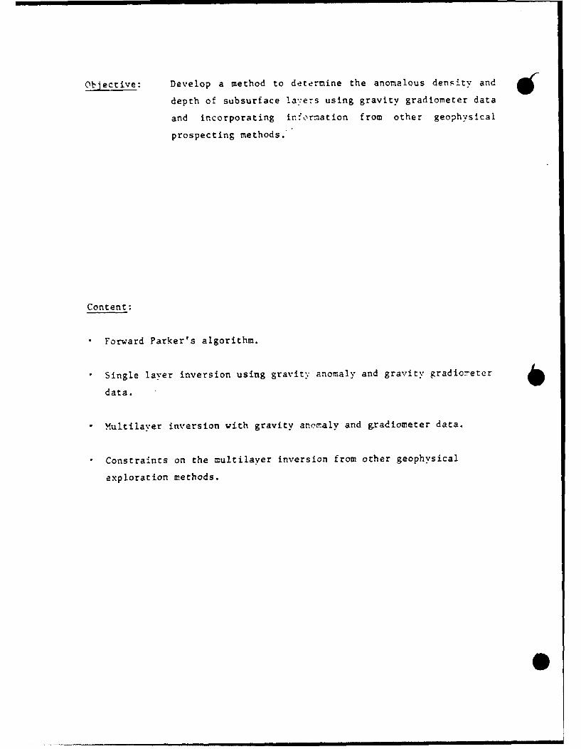
Objective: Develop a method to determine the anomalous density and

depth of subsurface la':ers using gravity gradiometer data

and incorporating information from other geophysical

prospecting methods.

Content:

" Forward Parker's algorithm.

" Single layer inversion using gravity anomaly and gravity gradioreter

data.

" Multilaver inversion with gravity anomaly and gradiometer data.

* Constraints on the multilayer inversion from other geophysical

exploration methods.

I. Forward Parker's algorithm

If F{ Fourier trarnsforrn of }G Newton's gravitational constant

c(x,y) density

z altitude at which gravity data are observed

h(x,y) :layer topography

T anomalous gravity potential

Ti. second-order gradients of T

u,v :spatial frequencies in the two directions

then:

-2,Tqz 0 cc(rn-1F{Tg(x,v) = 2Ge z no F(x,)h (.x,)l

n=1

-2FTq (xv) Go2 (2irg) P'-I 2Tru 2 nxx -n=1 noq

PT (x,v)I = -2.G (2;rg) n-IVV rI no q

*zz n o n

0, n-V{T xv(x,v)! = -2G E n2og 'rrtuv FP(x,y)hn(x,y))

-2Tqz O _

V~T (x,v)l = -27Ge o -"~g 2u KP(x~y)h~(~~xz nl n

-'-qz 'C(27 qn-IF{T YZ(x,y)l -2r(Ge no n!(~g F 0 xyh (x,v)}

j is the is'aginary unit.

ro I io-T I

Single Layer Inversion

Assume gravity anomaly data are available and have been corrected for

any thin sediments or water overlying the layer. Also assume that the

density varies in some smooth fashion reasonably known. Then the laver

topography h(x,y) is determined from

2-rqz 0

F{o(x,y)h(x,y)! = F{AE(x,v } e (2___ n -__,

2-G - F{ (x2ih~xg))

n=2 (1)

* Use equation (1) in an iterative inversion. Start with some estimate

of h(x,y) (probably given from borehole surveys), compute R.H.S. of (1)

up to n=N, then compute L.H.S. and take its inverse 2-D FFT to get

h(x,y). Iterate to achieve convergence. The degree n=N up to which the

sum in the R.H.S. of (1) is computed, is determined from the ratio

(SN /S 2).0x10-3 (with Sn= (2rq)n- i/n! F{hn(x,y)P(x,y)}). Convergence

in the iterative algorithm is considered when the r.m.s. of the

differences between two consecutive estimates of gridded h(xiY k ) is

smaller than 0.3 m.

• Excessive noise amplification in downward continuation is prevented

by low-pass filtering. For gravity anomaly profiles, it has been

suggested by Oldenburg to use cutoff passband frequency u0 :O.05Su 00.1

(cycles/profile spacing) and edge of the stopbard critical frequency

0.15!u S0.25.S

* For gravity gradiometer data higher limits for cutoff frequency up

and stopband critical frequency u have to be used, due to their high

frequency signature. Therefore less information will be smoothed out in

the downward continuation.

. The iterative inversion algorithm expressed by equation (1) converges

only for densities larger than a minimum density pmin * It also

converges for heights z0 minimum z 0 In short, convergence depends on

the density contrast, depth of the subsurface layer and the passband;

Ftopband frequencies of the low-pass filter.

Single Laver Gravity Inversion (continued)

Using gravity gradiometer data, we have six data sets instead of one

to determine the subsurface layer topography. Thus the determination of

h(x,y) is strengthened due to the additional infortation, and thus the

solution becomes more reliable. The equations for the iterative

inversion of h(x,y), using gradients T.. are derived from the forward

Parker's algorithm in the same way as for the gravity anomaly data.

Gravity Gradient Single Laver Inversion

• For simplicity assume T (x,y), Tyz (x,y), T (x,y) data.

• From the forward Parker's algorithm, after reconstructing the

equations

2.qz 1

F{ I(x,v)h (x,y)} = - [F({T xz(X,y)}/2rG~e

2 n-iF" nx)J2h(u F{o (x,yF)h{y }x2e

n=2

27rqz 1

Fthe(x,s)h(x,y)} = l FaTy z (x,y)/ 1 ThGie

(2rq) n - 1 (x,v)hn(xy) }n n! 12 1~I

2Trqz 1

FS ( (x,h (v)} S u= [F{ h zz (X,y)h/2Ge

cc 21(rq'n n

uvo (u,v)h (x,Y)n=2

•Iterate "or each one of the T xzTyzT zz data sets, to finally compute

three sets of subsurface laver topography h 1(x,y). Then combine the

solutions for h(x,y) from TsTlT using spectral weighting

1,1' ~ ~ x 1,2 1, z z z

F"h (x,y) }

S i l (u,v)F{h 1,1(u,v)} + S h2,2 (u,v)F{h 1,2 (u,v)} + S hl,3 (u,v)F{h 1,3 (u,v)}

S h 1 (u,v) + S h 12(u,v) + S h 13(u,v)

where hl, hi,; hl, ... solutions for h(x,y) from T T T1, 1 XZ, VZ z

respectively

Sh ; Sh ; Sh ... are the corresponding amplitude spectra.1,I 1,2 1,3

This iterative weighting procedure can be applied for more than three

data sets.

Multilaver Gravity Inversion

densitv co~ntrasts

*For simplicity we use gravity anomaly data. Assume a 4 layer model

on top of which a layer (composed of sediments, water) with density P1

is located. The density and bedthickness of layers 1,2,3 are known.

Determine the topography of the bottom lav.e r h(x,v:) having some

knowledge of the density 0.

" U'se Parker's formula for more than one layer

4 -2?wqz k (-) -VgxYl- 2IG E e n' VC k cNxy) h k(X,y)l (2)

k-l n-I

" Reconstruct the formula for multilayer inversion

VF; (x ,y)h h(X,V) 2

(3)

- t9'ag(x,y) - Ag(x,y')'/2,rGje n' Fl I~ (x v)hnI (x v)}observed others nm2 n '

Multilayer Gravity inversion (continued)

with 6g(x,y) determined from

others

4 -2 qzk G n-I

F{Ag(x,y)} = -2nG E eE F{a (xv)hn (x v)} (4)1 n!k kothers k=2 n= n

* Equation (3) is used in an iterative manner to solve for the unknown

topography h (x,y). Some apriori (or model) knowledge about h (x,y) is

necessary. This nowledge will provide the depth z

• The depth of each layer k,z is then determined by

z k+1 = zk - (bed thickness) k+ (5)Zkk+1

• The values of h (x,y) vary at each iteration, thus the depths zk need

to be updated. Due to this updating, the gravity anomaly Ag(x,y) will

others

vary as well. A reasonable starting model for tg(-x,y) would prob blv be

others

4

Z a kx,y)k=1

Ag(x,y) = Ag(x,y) (6)others observed

Z a k(x'y)

k=1

Combining equations (3), (4), (5), (6) an iterative procedure for

computing the topography hI (x,y) can be employed.

Multilaver Gravity Gradient Inversion

" Assume for simplicity that onl, T , T Vz, T are available.

" From the multi-layer formulation of the forward Parker's algorithm we

get after reconstruction of the formulas

2' qzIF{c(x,v)hI(x,y) - [F(T xz(X,y) - T (xy)/2rGje

observed others

(2rq)n- 2 nE j 27u F .c ( ,Y)h (x ,v)l

n 2

FJo (x,v)h (x,y)' = _ (F{T (x,y) - T (x,y)/27G]e 1

yz -yz

observed others

(2qz

FP o(x,v)h (x,v)} = - F{T x,y) - T (x)/2rG]e 1

xz -z

observed others

(2?rq~ n 1 , Y% )hln(X,Y)l

n= 2

where T xz(X,y), Tyz (x,v),T xz(X,y) are the gradients T xzTyzITzz

others others others

computed from the other three layers.

The same iteration procedure as for the gravity data has to be

applied for gravity gradient data. To combine the solutionsh ;h,;h for the subsurface topography from T ,T ,T1111,21,3 xz yz zz

respectively we use a spectral weighting scheme as in the single layer

case.

Multilayer Gravity Gradient Inversion (continued)

• After stripping the overlying layers, single layer inversion has

essentially to be performed. Deeper layer inversion can then be

attempted by examining a lower frequency band.

Again the advantage of using gravity gradiometer data is that five

more data sets are available with higher frequency content. Thus the

solution for h (x,y) is more reliable and more detailed for shallow

depths.

0

0

Constraints on Multilayer Gravity Inversion from Other Geophysical

Methods

* The inverted surface need not be the bottom one, as long as

information about the other layers is available.

. Densities from the other layers can be obtained from seismic data, or

from borehole surveys. Borehole data will provide density information

at two, or three points (maybe a few more) in the area of interest.

Then the densities between these points can be assumed to vary linearly.

* Information about bedthickness for each of the other layers can be

obtained from seismic reflection data or from well logs or from sonic

logs.

* If detailed information about the shape of each layer is not

available (as is often the case), then a reasonable approximation is

that the topography of the other layers varies in the same way as the

topography of the inversion subsurface.

* For the gravity correction due to the sedimentary layers, the density

(for Western Canada), is taken from extensive density logging as

P = 2.266 + 0.146 z ± 0.210 (gr/cm 3) (z: depth of sediments)

* Assuming known compressional (P-wave) velocities with depth, from

seismic traveltime inversion, a reasonable density approximation can be

obtained from the non-linear formula

P 0.23 V0. 5 (V : P-wave seismic velocity)

* >nformation about densities can alsc be obtained from deconvolution

of reflection seismograms and computed reflection coefficients. In this

case the density or velocity for some layer should be known (not the

upper sedimentary weathering layer though).

Magnetic Data-Relation to Gravity Data

For a constant ratio of density 0, to magnetic susceptibility k

0T - constantk

the magnetic anomalous potential W is related to the first order

gradients of the anomalous gravity potential T by the Poisson's equation

oH 0 7T with H : magnetic field strength

T u1 : magnetic permeability

* A similar relation can he developed between the magnetic field

anomaly B (B = - VW) and the second-order gradients of T. Inversion of

magnetic anomaly data resembles very much the inversion of gravity

gradiometer data.

. The ancmalv in the direction of the perturbing field !VB! is related

to the magnetic susceptibility by the relation

2r.N(u,v)qH Ole - 2 q z (2q)n-1 n )

0-n= n( F{k(x,y)hnCx,F{IB! =Uo n=1 n!" "

where the d iensionless vector N(u,v) is a function of magnetic

declination D and magnetic inclination I.

* information about the depths of the magnetized layers can be obtained

from the PSD of aeromagnetic intensity data, by using the method

developed by Spector and Grant.

S

Conclusions

. Forward Parkers's algorithm can be used to invert gravity anomaly and

gravity gradiometer data in an iterative mode.

• By using gravity gradiometer data, a solution can be obtained for the

shallower layers with better detail than for deeper layers for which

gravity anomaly data have to be used.

. Knowledge of depth and density of the overlying layers constrains the

solution for the layer topography.

* Depth and density information about the subsurface layers can be

obtained from either borehole surveys or inverted seismic reflection

traveltime data, or from density logs or from sonic logs.

• The same algorithm as for gravity anomaly and gravity gradient data

can be used for magnetic anomaly data, thus yielding magnetic

susceptibility values. Information about the magnetized layer depth can

be obtained from analysis of aeromagnetic data.

COMPUTATION OF THE GRAVITY VECTOR

*FROM TORSION BALANCE DATA IN SOUTHERN OHIO

by

Dr. D. AravelosDepartment of Geodesy and Surveying

University of Thessaloniki

Greece

Mr. Christian TscherningGeodaetisk Institut

Geodetic Department I

Gamlehave Alle 22

2920 CharlottenlundDenmark

ABSTRACT

The method of least squares collocation was used for gravity vector

estimation from torsion balance measurements in Southern Ohio. The results

were dependent on the covariance function used and on the selection of a proper

signal to noise ratio. Here a stanidard deviation of the noise of 10 E.U.

(10- 9 * s- 2 ) gave the best results. Expressed in terms of standard deviations

of observed minus predicted differences, the best results were 0.4" for deflec-

tions of the vertical and 2 mgal for gravity anomalies. This compares to signal

standard deviations of 4" and 22 mgal for deflections and gravity anomalies,

respectively.

p

COMPUTATION Of ]'HE GRAVITY VECTOR FROM TORSION B4ALANCE DATA'L

IN SOUTHERN OHIO.

by

D. Arabelo-,s arid C.C. Tscherning

Department ,-,f Geodaetisk Institut

Geodesy and Surveying Geodetic Departmert I

Univer-sity ,.t Thessaloniki

Greece Denmark

Abstract: The method of least squares collocation was used for gravity

vector estimation from torsion balance measurements in Southern Ohio.

The results were dependent on the covariance function used and ,_-n the

selection of a proper signal to noise ratio. Here a standard

deviation of the n,-oise of 10 E.U. (O-9*s - : ) gave the best results.

Expressed in terms of standard deviations of observed minus predicted.

differences, the best results were 0.4" for deflections of the

vertical ard 2 rgal for gravity an.i:malies. This compares to signal

standard deviations of 4" and 22 rgal for deflections and gravity

anomalies, respectively.

1. Introduction.

The method of collocation and similar optimal estimation techniques

have been proposed as possible methods for gravity vector estimation

from gravity gradi:,meter data, see e.g. Jekeli(1985). Since gravity

gradionieter data are no.t yet available, the estimation procedures hAve

only been tested usirg simulated data. However, the torsion balance

delivers measurements of the same kind as the gradiometer. namelv

l ine ar corabinators of secozrnd order derivatives of the gravity

p.:tr'tial (W).

P Using torsion balance data we may then demonstrate how least-squares

collocation (LSC) can be used for gravity vector 'est imat ion, and also

show which type of difficulties one may encounter while using the

rfietth.d.

Ir, o:rder to draw con~clusion~s fro~m the use of torsion balarice datatVrthe u.su of gratvity qr-adio:meter data, the data distribut io:ri ShouldW

corresporid to the one planned for the gradiorneter. Futhermcore gravity

vector, data must also: be available in the same area as the to:rsior

balance data. Such ar. optimal Situ ation is found in a 0.25 deg. * C). 75

deg. area in Southern Ohio, where gravity data, deflectiorns o:f the

vertical arid to~rsion balance data were o~bserved arid collected in the

peric:.d pr~ior to: 1970. The data is somewhat sparser than the .:ne

planned f:r, gradi.:metry, arid the area covered is smial ler than the

typical area fo:rseen to be covered by som.re ho:urs of aerial grad i.:meter

mieasurefilrit s. Furt hermiore the data is riot observed at al1t ituLde, but at

ground level. Also: Sou~therrn Ohio is rio.t typical, since the area has rio

large height variations. However, irn art operaticonal situatiorn,

topographic effects will in gerneral have to be removed (and restored).

In this way all areas from the standpoint of the gravity field

variation will look like Ohio (Forsberg, 1984, table 6). Also the

gravity variation at an altitude of 0.5 - 2.0 km will riot be riuch

di fferent from the variation at ground level, when topo~graph ic effects.

have beens removed. Furthermore, as we shall see, arn increase irn the

data deni ity would probably not have improved the quality *:f the

pred ict i .:-r vect or.

Deflectio:n of the vertical estimation have been successfully tested in

Southern Ohio by Badekas and Mueller (1963), using a simple rnumerical

integration maethod. With LSC we should be (and have been) able to

obtain similar results, the advantage being that the miethod riot only

enables the estimation of the gravity vector at points where the

measuremients have been made, but also in all points within a certain

distance fromn the measurements. LSC permits the est imat ionr of the

prediction errtor as well.

In section r':' we will introduce the available data, arid ir, section 3 we

will describe the use of LSC, and the associated process of estimiating

the so-called empirical covariance function. The results obtained

using var-i.:.uAs combinations of the data as well as different analytic

miodels f.r the emipirical covariance furnct ion are described in sect ion

4.

:. The Southe'r, Ohio test data set.

* Let W be the gravity potent al and U a corresponding reference

(riormal)p,:tential. Then the ar.,'malous gravity potential is the

differ-ence T = W - U.

The long-wavelength part ,of W ( or T) is described down to a 1 deg.

resolutior, by one :f the available spherical harmonic expansions

complete t.:. degree and order N=18C' such as the OSU81 arid the GPM2

c,-,efficiert sets (see Rapp(1931), Werzel(1925)).

Free-air gravity ariomalies (Ag) have beers published by Heiskarer, arid

Uotila (1956), ard deflectiors of the vertical (4,1)) by Mueller arid

Preuss (1965). They are in spherical approximation related to T

thr:,ugh the fo-,l lowing equatl,-,rs (Heiskaner and Moritz, 1967).

aT 2Ag = FT (1)

1 aT

1 1 aT= -rcospy ax

where o is the latitude, X the longitude, Y norrmial gravity and r the

distance frormi the origin, which ir, spherical approximation is obtaired

as the sum of the Earth mear, radius and the height. Torsion balance

data are published by Badekas(1967), and their relations to: T are

T - T (4)a x aZ

T &2T (5)

T T*:r y = :" 82 (6)

xy xy

a2T a2 TTA =

ay ax

4

where (x, y , z) are the coordinates of a local-I eve 1 coord i nat e syst em

with x east, y north and z up. The distribution of the torsion balan@

data is shown in Fig. 1.

Digital topographic heights was not available. However, topographic

effects have been published for the torsion balance in the same

publication as the observations and for the deflections in Badekas ard

Mueller (1968). The topographic effects on the gravity data riay be

calculated using the simple Bouguer plate reduction, since the terrain

corrections are rather srmall due to the smooth topography.

The use of the spherical harmonic coefficients within the frariewor-k of

LSC is equivalent to subtracting the contribution of the coefficients

from the data. Since the data used for the determination of the

coefficients primarily are free-air gravity anorsialies, the

coefficients also reprensent the attraction of the topographic masses

down to 1 deg. resolution. Consequently only the effect of a Bouguer

plate referring to the mean altitude of the topography (265 m) must be

subtracted from the gravity anomalies. However, this creates an .

inconsistency between the topographic corrections for the gravity data

arid for the other data types, which as we shall see later will result

in biases in the predicted results using topographic reduced data.

This problem is easily avoided in practice, if a detailled topographic

model is available.

Table 1 shows the statistical characteristics of (1) the "raw" data,

(2) the data from which the contribution from a set of spherical

harmonic coefficients (GPM2 to maximal degree 180) have been

subtracted and (3) the data (2) minus the topographic effects. Also

statistics for a subset of the gravity data located in an area close

t,-- the torsion balance data is giver, in the table. These 12 gravity

values have also been used in the following when comparing observed

arid predicted quantities.

Note the striking difference in the mean values. In fact, the area is

l,:,cated on the top and east of a large anomalous mass. Also note, that

the deflections of the vertical have beers transformed from NAD192.7 to

the preliminary NAD33 using datum shifts parameters provided by the

U.S. National Geodetic Survey. The gravity values have beers

transforrmied fro:mrs the Potsdam system to GRS198o usirng a bias c.:rrc-cti.-.r

of 13.7 magal. Hence a small bias with respect to IGSN 1971 may still

be left.

3. Least-squares collocation and covariance functions.

The theory and practice :f LSC is described in numerous publicat i.,r,;.

A recent survey is giver, ir, Tscher-nirg(1985b).

Suppose we have givers r observations related to the anorralous gravity

field through r linear furctionals (eq. (1) - (7)) ,

L. (T) = yI + ei, i = ... . n.

Here e. is the noise or error. Then let C. . denote the covariarnce1 1 .)

between L i (T) and L (T) and CLi the covariance between the value ,--f a

linear functi.-ral L applied or the anomalous potential, L(T), and

L (T). We then obtain an estimate L(T) of L(T) as

T -1L(T) =(C } (C.. D.} {y} (2)

Li i

where D. . is the covariance of the noise associated with the i'th andIi -

J'th observatiors. Let C denote the sum of the C. . and D. matrices. _

Then an estimate of the mean square error for a linear functional is

obtained by

,'r -1Ca (L(f) - L(T)) = CLL - C C CL

where C L is the vector of cc-variances between the observatiozns and the

quantity L(T) and CLL is the variance of this quantity.

Simlilar equatiors are obtained if, instead of the observati.-ns y, we

use the values from which we have subtracted the effect of the

topography or the contributior from a spherical harmonic exparsior. Or,

the right hand side ( of eq. (8)) the covariance function will be the

ore associated with these residual observations. The vector of

6

observations will conrisist of these residuals arid oi the left hand side

we qet the r:sid,.tal potential, to which in the final step W_ shosuld

add back the p,:.tertial implied by the tc.pgr-aphy arid the spherical

harmonic expansion. In the case we :nly have .'jubtracted the

contribution from GPM-, we will associate a superscript "s" with the

relevant quantity, and if also the topographic effects have beer,t

subtracted we will use the superscript "t", i.e. Ag

The starting point for the use of LSC in a local area is the

cc,.mputation arid analytic modelling of the empirical covariance

function. Its estimatiorn is discussed in detail in Goad et al. (190-4).

Numerically the estimation is simply done as the computation :f the

mean value of products of quantities lying within the same interval of

spherical distance. The size of this interval is called the sampling

interval. F,:r vector quarntities, like comporents of deflections of the

vertical, the components of the horizontal gravity (disturbance)

gradient ( eq. (4), (5)) and the mixed second order derivatives (eq.

(6), (7)), the products are formed between products of "along-track"

and "cross-track" components. For details, see Krarup and Tscherning.

(1984).

The quality of the estimation depends on the size of the sampling

error, the regularity of the data distributior and the data error. The

size of the area should also be so large that the mean value of the

quantities (from which the contributiorn from the spherical harmonicS

expansion, here GPM2, have been subtracted), yi , is -zero. For a

spherical harmonic expansion to degree 180, this generally will be

achieved for a 1.5 - 2 deg. equal angular area, since mean values of 1

deg. blocks have been used for the computation of the coefficients.

For the approximately 1 deg. block surrounding the torsion balance

data the mean value of the available 22*7 Ag -values is -3.3 regal (cf.

Table 1). Since the stardard deviation is 19.8 rgal, this meat, value

is not significantly different from zero. The gravity values in this

area were therefore used for the estimation, of the covariance

function, b,:th using Ag s and Agt values (cf. Fig. 2 arid 3).

7

When est imat irg cr,ss-covariarce furct i:ns with the torsion balance

data, we havo the pr.obleni that the data covers a much smaller area.

* Futher,m.:,-e (cf. Table 1), the gr-avity variation in the 0.75 deg * 0.85

deg. area is significantly different fr-om the variatior, in the ar-ea

immediatly s.,r,':.urid ing the torsiorn balance data. Here the variation 1 'a

,.uch larger, and the mean values are nor: -- ero. We decided anyway to

estimate empirical auto- and cross-covariarce functions between the

(GPM- arnd GPM2_ + terrain reduced) gravity and torsion balance data.

Figures 4 to 12 show the covar-iarce furct.ons for" the GPM- reduced

data. It should be rioted that the mear values have not beer, subtracted

f-ro, the data.

The modelling of the ermipirical covarfiance function is based or, the

fitting of an analytic expression to the empirical values. We used a

model for, the gravity aromaly covariarce functior, developed in

Tschernirg and Rapp (1974),

Rz

C(P,o) = AO-1) 8 i+2 , ) O10Pi = 181 T i Z'( +1) (csrF (1P)

with the two free parameters A and R In this expression r' is the

distance of the point 0 from the otigin, P. the Legendr-e-polynomial :,f1

degree i, 4e P ' the sph2rical distance between P and Q and R B is the

radius of the so-cal led Bjerhammar sphere. The summation starts from

181, since we have subtracted the effect of GPM2 to degree 180. This

is equivalent to presupposing that the coefficients are error free, a

hyp:thesis which is certainly not true. However, the consequence of

adoptirg the hypothesis will mainly be seen in predicted geoid

heights, see Prabelos(1980). Also the start of the summation from

i=120 made it reasonable to introduce a modification, namely the

division by i+4 instead of a divisiorn by i+24 in eq. (10) as

rec.:,rmerided in Ibid. (1974). This modificati:.n gives so, me corputational

savlings.

The factor A ir eq. (9) is linearly related to the value at spherical

distance :et-_-,, the variance. The value of RB is more difficult to

estirsiate due to the uncertainity in the estimation of the covariances

0

ard the weak relationship between RE and the covariances, see

Tscher'ning (1985b).We decided to try to find the best one (within the

class ,:.f furictirs giver, by eq. (10)), siply by carrying out

prediction experirmierts with differernt values of RB, and thern selecting

the ore, which gave the best agreement between observed and predicted

deflection values. The results are surmmarized in Fir_. 13 . The

analytic covariance furction found using this procedure

had a depth to the Bjerharsimar-sphere of 3.0 krii. Its graph is shown

with the empirical values in Fig. 2 - 12.

It should be rioted that this procedure of selecting a covariarce

furicti : rs,,:del very well could have beer, used if only torsion balance

.:r- gradiometer data had beers available. A subset of the observatiors

could have beer, used as test-quantities and the relaining observatiors

as the giver, data, The covariarce rodel, which gave the best results

irs a least squares sense msust then be the one in between the used set

of rsodels, which is most close to the true empirical covariance

funct ion.

4. Prediction tests and results.

For the evaluation of the predictions (eq. (8)) as well as the

calculation of error estimated (eq. (9)) the FORTRAN program GEOCOL,

(Tschernirg, 1985a) was used.

Ir, order to check the consistency of the gravity vector data, we first

predicted the deflections at the 8 sites shown ir Fig. 1 from the 227

gravity values and subsequently the 12 gravity values in the vicinity

,-.f the torsion balance data from 15 pairs of deflection points in the

arose area as covered by the 227 gravity values. The results are given

irs Table 2. Note how surprisingly well the gravity anomalies are

determined fr,:,, the deflections. Also note, that the deflections are

predicted just as well fro.m the gravity data as from the torsion

balansce data, as we shall see later.

We tlien wanted to predict also the torsion balance data from gravity,

torsion balance fro,i torsion balance data and gravity and deflections

from torsion balance data. We assigned a noise standard deviation of

9

I.Q E.U. to the tlt-sion balance data, equal to the value given in

Eadekas arid Muel e- (1968, p. 6871). However all our resul t, were

* "bad", in the -er,.;c that the error estimates c,:mputed usi rg eq. (9)

were much smaller than the variance of observed minus computed values.

We ther, spent 14 days intensivly c:-.-ckirng GEOCOL, but found no

significant err.or. This made us go back to the publicatiorn

Badekas(1967), which contains detailed maps showing the individual

data in vector-like f,:r-m. This revealed that neighbouring values could

be rather" differernt, signifying a much larger error level than we h..d

expected. Also the er.mpirically estimated auto-covar-iance furctions

irdicated that a rather large noise was present. This car, bu seer, fr',:.r

Figures 8 to 11, where the variarce is much larger (around 1o')C E.U.)

than the value fourd by sro:,thly extrapolating frorf the first 2 - 3

empirical values t:, the value at spherical distance zero (the

vat iance).

Then changing the noise variar.ce to 100 E.U. , we suddenly obtained

consistent results. This value is probably too pessimistic, but not

irp_,:ssible (I. I.Mueller, personal communication, 1986). We thern tried

using changing noise levels. The results are illustrated in Fig. 14

16. In fact values of the noise between 50 and 150 E.U. all give

rather- similar prediction results, but 100 E.U. a gave the best

results. We thern used this value in the following computat:rns.

Having arrived so far, we decided to make a series of computational

experiments, which should illustrate the dependence of the prediction

result or,

(1) the rmodel selected for the covariance furctior

(2) the use :.r nora-use of the topography

(3) the data type and che combination of various data types

(4) the data dersity.

The Jependerce on the covariance function as mentioned already has

been used to select a "best" analytic model. The dependence :'n tho

m:-odel (the depth t:, the Blerhar,,mar--sphere) is illustrated i, Fig. 1..

The use of tp.:.graphic data results in a slight smoothing of the

qravity field data (cf. Table 1), and we should expect a similar

irprcoverert of the predict ion results. However, as seen from Table 3

not very much is gained, but this is probably due to the high data-

density. The t.-.pographic information is a-priori well represented by

the data.

In order to see the influence of the data density we used either all

data points or one value from each 2'*2' cell. Using all data gave

only a small impr'ovement as seer, from Table 3. More interesting is the

clear- difference in conrtributior from the various torsion balance

eco-:p,.nernts to the components of the gravity vector. We maybe should

expect the significant contribution of the horizontal gradient of the

gravity disturbance to the deflection components from geo:,etrical

reasons and from the results presented in Table 2, where gravity data

were used to predict deflections. The rixed second order derivatives

contributes little, but anyway something of significance.

It is clear that we can not estimate the abso-lute values of the

gravity vector components fro-m torsion balance data alone. This is

also confirmed, since we get relatively large biases (cf. Table 3).

However, gravity vector differences are well determined as seer, from

the small standard deviations in the table. On the other hand, we can

easily add observed gravity vector ineforrmation to the input data in

LSC. We selected one of the deflection points, which coincide with one

of the points of the torsion balance network, but we had to select a

gravity station at some distance ( 1 km ) from the network. The result

is given in Table 4. We see that most of the biases have decreased,

but the bias in the topographically reduced Ag has increased. The

reason for this rmlay as mentioned be due to the inconsistency of the

topographic reductions.

Cornt..ur plots showing the predicted gravity anonaly and deflection

cormpo.nents with the esti reated er-rors of predict i.on (eq. (9) ) are shown

in Fig. 17 ,- -/"

5. CoriclI us i on.

We have seer, ho:w LSC is suitable for gravity vector est im~at ion. in a

local area frcrsm nradi':reeter-l ike data. If the riethod should be used

econom~ical ly for data distributed over large areas, then. the Prea must

be split in, sub-areas o:f reasonable size.

The results r:btairaed in the best cases ( 0.4" for deflectiorns and 1.6

m~gal for- gr-avity arcrili~)is very encouraging since the grad i,:reter

is supposed t. have a n~oise level below 1 E. U. However, as we have

seen, it is imiportant to 1Ae a reasonable signal to noise r-.t io.

The proper removal .:f biases, using observed comipornents or the gravity

vector, requires sorte futher invest igat ions. Here a data set co:verin~g a

lar-ger area would be sui table, permittirng the proper est imat ion *:f all

cr-o-ss-covar i ace functi ons.

Acknowledgement: This work was carried ClUt while the first author was

a visiting scientist at the Geodaetisk Institut, Dernmark.

Re ferences:

Arabe los, D. : Urit er-suchusgen zur gray irmetri scher. Geoi dbest irtmm'rig,

dargesteilt ami Testgebiet Griechenlarid. Wiss. Arb. d. Fachricht ung

Verritessurigsweser, d. Unixversit aet Hanno.:ver, Harnni:ver 1 '9-0(.

Badekas, J.: To:rsx.n Balance Observat ion.s in Sou.thwest Ohio. Repo:rt .:f

the Departm~enit .:,f Geodetic Science, Report No. 89, The Ohio: State

Urniversi ty, Co:lumibus, 1967.

Badekas, J. arid I. I. Mueller: Interpo:lat ion of the Vertical Deflect ion

fro:m Horiz.:.ntal Gravity Gradients. J. Ge.:phys. Res., Vol. 73, N.:. -1,

pp. 68069-607-0, 1968.

Fortsber-g, R.: A Study of Terrain Reductions, Density Anomalies arnd

Geophysical Inversion Methods in Gravity Field Mocdelling. Repo:rts

o:f the Departmienit of Geodetic Science arid Surveying, No. 355,

The Ohio State University, Columbus, Ohio, 1984.

Goad, C. C., C. C. Tscherniag arid M. M. Chin: Gravity Empirical Covarianice

values for the Continental United States. J.Geophys.Res., Vol. 89,

No. B49, pp. 7962~-7968, 1984.

Heiskaien, W. A. arnd H. Moritz: Physical Geodesy. W. H. Freeman & Co-, Sari

Francis:, 1967.

Heiskaien, W.A. arid U.P. Uotila: Gravity Survey of the State .:f Ohi.

Inst itiute of Geo:desy, Photogrametry arid Carto:graphy Publ icat io:n, No.

6, The Ohio State University, 1956.

Jekeli, C. :On Optimal Estimation of Gravity from Gravity Gradients

at Aircraft Altitude. Rev. oif Geophysics, Vol. 23, pp. 301-311, 1985.9

13

Krarup, T. and C.C. Tscherning: Evaluation of Isotropic Covariance

Functions of Torsion Balance Observations. Bulletin Geodesique,

* Vol. 58, n,-,. 2, pp. 180-192, 1984.

Mueller, I.I. and H.D. Preuss: Astro-Geodetic Deflections in Southwest

Ohio. Rep. No. 61, Department of Geodetic Science, The Ohio State

University, 1965.

Rapp, R.H.: The Earth's gravity field to degree and order 180 using

SEASAT altimeter data, terrestrial gravity data, and other data.

Reports of the Department of Geodetic Science and Surveying No. 3222,

The Ohio State University, Columbus, Ohio 1981.

Tscherning, C.C.: GEOCOL - A FORTRAN-program for Gravity Field

Approximation by Collocatiorn. Technical Note, Geodatisk Institut,

. ed., 25 MAR 1985a.

Tscherning, C.C.: Local Approximation of the Gravity Potential by

Least Squares Collocation. In: K.P.Schwarz (Ed.): Proceedings of

the Irternational Summer School on Local Gravity Field Approximatior,

Beijing, China, Aug. 21 - Sept. 4, 1984. Publ. 60003, Univ. of

Calgary, Calgary, Canada, pp. 277-362, 1985b.

Wenzel,H.-G. : Hochaufloesende Kugelfunktiorsmodelle fuer das

Gravitationspotential der Erde. Wiss. Arb. Fachrichtung

Vermessungswesen der Universitaet Hannover, (in print), 1985.

7 i,"" 1 6. /'% col" s ,,e- ,1-,. 2- 64 v

0 /mmmmm ~~~~~~~~~~~~~ ouTunnmn 4Snsuun Ilnnunnmum mm lnUNmN

14 6Figure captions.

Fig. 1. The distribution of the torsion balance (+), gravity data (e)

and deflections of the vertical (o), with the free-air

gravity anomaly field contoured at 2.5 mgal interval.

Fig. 2. Empirical (solid line) and synthetic (broker line) covariance

functions for the gravity anomalies in Southern Ohio. GPM2

-ere0oved from the original data. Units nigala.

Fig. 3. Empirical and synthetic covariance functions for the gravity

anomalies in Southern Ohio. GPM2 and topographic (sirm ple

Bouguer plate) effect removed from the original data. Units

mgal

Fig. 4. Empirical and synthetic cross-covariance functions between

Ag and T . Units higal*E.U.

Fig. 5. Empirical and synthetic cross-covariance functions between

Ag and T4 . Units mgal*E.U.

Fig. 6. Empirical and synthetic cross-covariance functions between

2*Txy and T A. Units E.U.

Fig. 7. Empirical and synthetic cross-covariance functions between

Ag and 2*T . Units mgal*E.U.Ky

Fig. 8. Empirical and synthetic auto-covariance functions for the2

T component. Units E.U. .

Fig. 9. Empirical and synthetic auto-covariance functions for the2

T component. Units E.U.

Fig. 10. Empirical and synthetic auto-covariance functions for the

2*T coroponent. Units E.U.

Fig. 11. Empirical ard synthetic auto-covariance functions for, the

T component. Units E.U.''

• I a | | |L

15

O Fig. I :'. Erpirical ard synthet ic cross-covariarice f'irct ions betweer

Txy and T A. Units E.U. -

Fig. 13. Dependence of the prediction results (expressed in terrmis

of standard deviations of differences observed minus

predicted quantities) or the covariarce functior ( the depth

to the Ojer-harirsar sphere). x = t = -. Topographic

reduced data shown.

Fig. 14. The effect of changing of the noise level on the predictior

results of gravity anomraalies from torsion balance data.

(expressed in terms of standard deviation of differences

observed minus predicted). A = unreduced, x = topographic

reduced data.

Fig. 15. The sare effect as in figure 14, for the 4 component

of the deflection of the vertical.

* Fig. 16. The same effect as ir, figure 14, for the n component

of the deflection of the vertical.

Fig. 17. Prediction of gravity anomalies from torsion balance data.

(Contour interval is 5 regal).

Fig. 10. Error of prediction of gravity anomalies frc~m torsion balance

data. (Contour line interval is 0.25 mgal).

Fig. 19. Prediction of a form torsion balance data. (Contour interval

is 0.5 arcsec).

Fig. 20 . Error of prediction of g frost tor-sion balance data. (CnrtourU

interval is 0.25 arcsec).

Fig. 21. Prediction, o:f -n from torsion balance data usirg eq. (9).

(Contour, interval is 0.5 arcsec).

Fig. 221 . Error of prediction of n from torsion balance data. (Conto:.uriinter-val is 0'.25 A,-csec).

16

Table 1. Statistical characterisi.cs of the raw and reduced data

227 gravity points, 12 gravity points, 8 pairs of deflections

of the vertical and 233 points of torsion balance observations)

Dat a-GPM2-

Raw data Data-GPM2 topography

standard standard standard

mean deviation mean deviation mean deviatior

Ag (,,igal) * -1.24 22.20 -3.32 19.81 -3.32 16.74

Ag (mgal) ** 22.64 27.66 16.31 25.98 16.24 22.41

(arcsec) 0.92 1.44 0.98 1.49 -0.12 1. 70

(arcsec) 4.41 4.72 4.84 4.74 5.89 4.7'

T (E.U.) -0.56 16.20 -0.52 16.24 -1.07 14j

T (E. U.,) -8.69 20.59 -8.73 20.63 -7.89 19.40yz

T (E.U.) -0.35 22.62 -0.37 22.65 -1.12 20.10

2*T (E.U.) 2.38 19.70 2.38 19.74 2.43 17.53xy

• 227 points ** 12 points

1 7

e a T.bl I.e Prediction resImlts

of the two contporaents of the deflec- of 12 gravity val1uesfi:.i

tior, at 8 Points fromr~ ;227 gravity of deflection vilues

po i rts irn 15 po~ints

------------------------------------------------------------------------------------

Ag

obs. - pred. obs. -pred.

riput st andard st and ard st and ard

(i t ta r.ear. deviation mnean~ deviation mean d ev iat in

(arcsec) (arcsec) (mg a I)

-.irreduced .03 Cf.71 -0. 17 0.43 5. 20 4. 3 2

t op -: gr.

reduced -1.27 0.47 1.56 0.47

-I- -----------------------------------

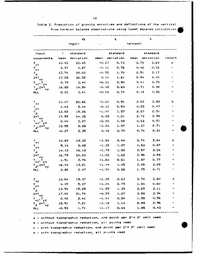
18

Table 3. Prediction of gravity anomalies arid deflections of the vertical

from torsiors balance observat ions using l east squares col .cat 1or

Ag n

(riga I) (arcsec)

Input * standard standard standard

components mean deviation mear deviat ion mean deviation remark

T 10.43 22.45 -0.27 0. 73 .. 70 3.69 a

T 4.97 4.87 -0.12 0.76 0.40 0.72 -

T 13.74 0.03 -0. 95 1.70 2.51 3. 17 -

*T 17.28 26.58 0. 14 1.21 2.84 4.00 -My

Tx , T 0.79 3. 40 -0.3 0 " . 90 0. 41 0.70 -

T3,T 16.85 14.94 -0.45 0.60 1.71 2.92 -

ALL 5.03 3.41 -0.04 0.74 0.13 0.56 -

T 10.07 22.66 -0.-0 0.91 2.62 3.38 bxz

T 4.43 5.44 -0. 12 0.50 0.55 0.47 -yz

T 12.68 19.26 -1.07 1.57 2.57 2.91 -

2*T 17.59 24.38 0.28 1.21 2.72 3.98 -xy

T , T 0.04 3.27 -0.20 1.08 0. 68 0.52 -x:' yz

T , 2*Txy 15.55 8.28 -0.24 1.07 1.37 2.71 -

ALL -0.27 2.35 0.48 0.70 0.74 0.31

T 10.89 19.32 -1.54 0.44 3.74 3.64 cMz

T 5.14 5.08 -1.32 1.07 1.83 0.87 -yz

T 14.13 16.13 -1.79 1.50 3.57 3.24 -

2*T 16.79 24.03 -1.05 1.22 3.96 3.99 -xy

T , T> 1.51 2.74 -1.64 0.61 1.87 0.77 -

To, xy 16.44 13.21 -1.44 1.45 3.03 3.09 -

ALL 3.36 2.47 -1.5) 0.58 1.75 0.71 -

T 10.64 19.37 -1.35 0.63 3.70 3.30 dxy

T 4. 15 5.37 -1. 24 0.79 1.84 0.60 -Yz

T 13.94 15.29 -1.89 1.39 3.65 3.11 -

2*T 17.00 21.74 -0.29 1.27 3.38 3.94 -xy

T , T 0.42 2.41 -1.41 0.80 1.95 0.56 -MZ y:

TA 2.T y 15.91 7.21 -1.18 1.14 2.89 2.96 -

ALL -0.93 1.71 -1.17 0.44 1.85 0.43 -

---------------------------------------------------

a without topographic reduction, one point per 2'. 2' cell used

b without topographic reduction, all points used

c with topographic reduction, one p.int per 2'* 2' cell used

d with topographic reduction, all po:ints used

19

Table 4. Prediction results using all torsion balance data and

in addit ion o:ne gravity poin~t arid orme deflect ion point

(rsgalI (arcsec)

i npu t standard standard starndard

data mear, deviation reeare deviation miean. deviat it-ri

.rweduced C). 05 .150.2~6 C) 6 . 0' 21 C. 370:

tc'popcgr-.

reduced - 5. 137 2.40 -0. 06 0.49 0. 55 0. 61

q - - - - -- - - - - - -- - - - - - -- - - - - -- - - - - - ---5- - -

ft.0

cza

or. CD

of- -2

01

aa

000r

CA c

ot"

cl#

ita

0

Ps I OE .

Fig. 2

0

0-O .4 0.0 0 0 0.40 O-s

.i .

Fig. 6

........

a-o01 .0 0.0 C'o aS

PSI lol.4-i.

~C2

a0

P3 I EG.

0

0.00 0.10 0.20 0.30 o 0.an Oso

P31 I'0(0.)

Fig. 8

0tCc

6

0 lc 01 o 0.0 O'o OS

101 f~ .

Fig 10

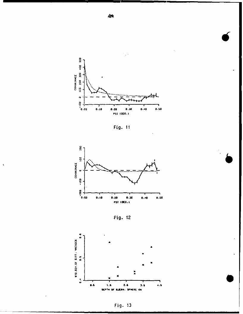
C,)

O-' 0.0 02 0j .0 05

s0 I

o JC.).

Fig. I1I

PS.. C.).

• -.-.

............

- - -- -

0

*1 5

0.00 0.10 0.20 0.30 0.40 0.60

PSI t0ECC

Fig. 12

U

0.15 I .S 2 .$ $ .Ai 4 .6

*CPT" Ow sIcWiI,. sr" (44. i"

Fig. 13

Ia

ao

aC!

M-*vc NOS N

Fig 14

x a

0. 3 a . LC 1 -SIaLA SILEJ

0.0 3.0 6.0 9.0 I2.0 IS-0

SiO-C .cc.f "OISE c.u.

Fig. 16

Crd)

01 1

M*

10 - c

0* 3 Co

01 0.

OC 0

0, 00

(n- (0rC? 0 *0 Ns,,

20 -C (n

0 . 0 ° 0 .

00 0)

C))

4 CO

ene

OD

at *

0** * a

U. 4

O** 44O4

, .. . -... ,

O " *

9-

4,,,

O ") 4"* O "

0. 0. 0cn a)

/ 0.

C'.D0.

Sn c

++ 00

co C

C,

0** +*0

0. 0Sn n S

co (n

(.0)

0 c

co . . 4 *CC)

(1 en . 4

* 4 4

9 4 4 -

0* - 4 0

(r) ~ ~ ~ ~ + +_____ 4

++

cz4

oc

+ 4-- +

o 4o

(4))

%k 91 , .-

c "C

r. (. 0 l

CY) ____ - - C'

0. 0. 0a) )

600

9.0

99

00-.

0.

0 0 001

0. 00. It(WI-n ,

0. Il0

0) 0) a)

0

c,.) +_ _ _ _ _ _ _ _

+ e4

4c

ca *

C.- (0 . Ij

++ ** +* 0* +

0. 00.0m,.

ESTIMATION OF GRAVITY VECTOR ODMPONENTS

FROM BELL GRADIOMETER AND AUXILIARY DATAUNDER ODNSIDERATION OF TOPOGRAPHY AND

ASSOCIATED ANALYTICAL UPWARD ODNTINUATION ASPECTS

by

Dr. Hans Baussus von LuetzowDepartment of the Army

U.S. Army Engineer Topographic Laboratories

Fort Belvoir, VA 22060-5546

ABSTRACT

Following an introduction, the paper briefly discusses gravity gradiometer

applications. It outlines the estimation of first order derivatives of the

anomalous gravity potential from Bell gravity gradiometer and auxiliary data in

the context of a Weiner-Kolmogorov optimization scheme under consideration of

computable "topographic noise", accomplished on the basis of the Pellinen-Moritz

solution of the boundary value problem of physical geodesy. The paper also

addresses four different methods of analytical upward continuation of first

order derivatives of the anomalous gravity potential under identification of a

finite difference method using Laplace's equation as the most economical and

efficient one. Relevant conclusions are then presented.

1. INTRODUCTION

The estimation of gravity vector components from Bell gravity gradiometer

and auxiliary data has been discussed by a nunm:r of authors, including Jordan

6(1982), White and Gol4stein (1984), Center, Jordan and Peacock (1985), and

Baussus von Luetzow (1985). Apart from gravity gradiometer self noise power

spectra or corresponding covariance functions, the collocation theory of

physical geodesy was employed to derive spectra and cross-spectra or equivalent

covariance functions involving first and second order derivatives..Qf the anomalous

gravity potential. The basic covariance functions, pertaining either to a

randomized anomalous gravity'potent'fal or.to a randomized gravity anomaly,

accomplished by the subtraction of low frequency harmonic representations of

anomalous potential or gravity anomaly data, presuppose the existence of homogeneity

and isotropy. The application of collocation theory does not face difficulties

in the case of quasi-flat terrain and is a prerequisite to

arrive at small estimation errors for gravity vector components

in the context of an airborne survey over a square area of 300 x 300 km' , coveredwith parallel traverses and cross traverIes 5 km apart, conducted at an elevationof 600 m at a speed of about 360 km hr , and employing only a limited amount ofmeasured gravity vector component data. It is., however, well known that theassumption of homogeneity and isotropy does not satisfactorily hold in the presenceof moderate to strong mountainous terrain. Some efforts have been made to apply

heuristic topographic corrections to gravity gradiometer measurements. Still,the problem remains to provide for a Wiener-Kolmogorov-type estimation processfree of computable topographic noise so that the assumption of homogeneity andisotropy is reasonably fulfilled with respect to modified, signal-type measurementsdisturbed by gradiometer self noise only. The solution to this problem ispossible under application of approaches to the geodetic boundary value problemand the correlated interpolation of gravity anomalies and deflections of thevertical in mountainous terrain by Pellinen (1969), Moritz (1969), and Baussusvon Luetzow (1971, 1981). Section 3 as the main section of this paper addressesthe solution under consideration of the estimation process and the computationof "topographic noise". The preceding section addresses in a compact waygravity gradiometer applications to place the determination of gravity vectorcomponents over relatively large areas and the analytical upward continuationof vertical and horizontal derivatives of the anomalous gravity potential inthe proper perspective. The relatively short sections 4-7 discuss differentmethods of analytical upward continuation, followed by several conclusions.

2. GRAVITY GRADIOMETER APPLICATIONS

Geodetic research and the development of associated technology has beenconsiderably stimulated by military requirements and actual or potentialmilitary applications with critical funding provided by the U.S. Government.The result thereof was an increase of scientific knowledge, new instrumentationand techniques, and technology transfer to the civilian sector, particularly innavigation and surveying.

The main applications of gravity gradiometers follow:

Establishment of the spatial gravity field in ICBM launch areas (most importantapplication). This includes gravity vector components on the ground forcalibration, local to global coordinate transformations, geodetic azimuthdetermination, and gravity programmed inertial positioning (beneficial toSmall ICBM or Midgetman). An accurate spatial gravity field, extending to

Intercontinental Ballistic Missile

2

a height of 200 km, provides also for comparisons/calibration for theGeopotential Research Mission (GRM) and a Superconducting Gravity GradiometerMission (SGGM). Instrument: Bell Gravity Gradiometer.

2o Accuracy enhancement of SLBE's Instrument: Bell Gravity Gradiometer.

o Improvement of global gravity field for geophysical applications (GRN).

Instrument: Superconducting Gravity Gradiometer.Byproducts: ICBM target error reduction (not critical), cruise missilenavigation, improved satellite ephemeris.

High accuracy space navigation. Instrument: Superconducting GravityGradiometer (six axis version).

0 Gravity vector densification over large areas for gravity programmedinertial navigation and for geodetic network adjustments. Instrument: BellGravity Gradiometer.

o Subterraneous mass detection (cavaties, oil, water). Instrument: Super-

conducting Gravity Gradiometer (vertical axis version).

* Test of Newton's square law and tests of Einstein's theory of relativity.Instrument: Superconducting Gravity Gradiometer.

3. DETERMINATION OF DERIVATIVES OF THE ANOMALOUS GRAVITY POTENTIAL OVERMOUNTAINOUS TERRAIN USING BELL GRAVITY GRADIOMETER MEASUREMENTS ANDAUXILIARY DATA

A. Notations and Relations Used

/ anomalous gravity potential

__ derivatives taken along the local horizon in a northern andi v eastern direction

n = sn/, Bell gravity gradiometer instrument noise with white noisecomponent , and red noise component 4a

signal variable indicator

topographic noise component of

ST topographic noise component of T

lover order spherical harmonics representation of T used forsubtraction

7 lower order spherical harmonics representation of ;r used forsubtraction

lover order spherical harmonics representation of 1 usedfor subtraction

2 Sea Launched Ballistic Missile

3

lower order spherical harmonics representation ofused for subtraction

T T F-A

Kweight factor with measurement index 1 and computationindex 4 , applicable to r in Wiener-Kolmogorov estimation

Kweight factor with measurement index and c, aputationindex J( , applicable to 7 in Wiener-Kolmogorov estimation

.r

earth's mean radius

unit sphere (full solid angle)

r length of radius vector from earth's center to a moving pointon earth's surface

length of radius vector from earth's center to a fixed pointon earth's surface

r length of radius vector from earth's center to a fixed pointon a level surface above earth's surface

-- )P -- -7rangle between radius vectors r and r or r

e r 7- -C

Cazimuth angle counted clockwise from north

S (.4-r)generalized Stokes Function

Aelevation of terrain referring to a movable point on earth'ssurface

4/ elevation of terrain referring to a fixed point on earth's surface

1A elevation of level surface above terrain

4

40= [I1~'A J planar-approximation to

gravity anomaly on earth's surface

c topographic correction to gravity anomaly

,64- A C Faye anomaly

Bouguer gradient

gravitational constant

standard density

potential of the topographic masses

,V. <'"/') d%9 with V as an arbitrary variable

gc

geographic latitude

0o~geographic longitude

B. Estimation Process

A Wiener-Kolmogorov estimation can, under consideration of / and Tonly, be characterized by

5

The derivatives / , also called truth data, are, of course also associatedwith measurement errors. With respect to deflections of the vertical,proportional to /.V and Ty , efforts are being made to determine themastrogeodetically with an error of 0.1 arcsec rms. Gravity anomaliescan be measured with a relatively greater accuracy. In order

to compute the vertical derivative = . , high degree spherical harmonicexpansions presented by Rapp (1987) or-the GRIM3-Ll Model described by Reigber,Balmino, Mll1er, Bsch and Moynot (1985) may be employed. These models arealso usefulfor the subtraction of lower harmonics components from measuredfirst and second order derivatives of 7

Regarding eq. (1), it is assumed that all measured quantities refer to alevel surface. In the case of quasi-flat terrain, /kK estimates have beenmade from r' on the earth's surface and from airborne 7 -measurements,employing spatial covariance functions. This is not possible in the presenceof pronounced topography. In this case, it is

where -- is a representative gradient obtained from gravity gradiometer

measurements. There is no significant degradation in accuracy if eq. (2) isused.

For simplicity, eq. (1) presupposes the prior application of quasi-systematiccorrections obtained from lower harmonic expansions. In the presence of Wpronounced mountainous terrain, eq. (1) is reformulated as

'oe

C. Computation of "Topographic Noise"

The essential task is the computation of topographic noise componentsof the derivatives , T , Z. respect, the solution nomenclature

Y z in 3this rsetemployed by Moritz (1969) is applied. In order to obtain solutions atelevation AA instead of solutions at elevation / 7 A ,Stokes generalizedfunction S replaces Stokes function rJ(5)in the solutions where applicable.

First, the solution for T at a point A is written asA

Moritz (1969), p. 31.4 is explicitly formulated by Moritz (1966). See p. 49.

6

IfI

The solution components are

T/ represents the "signal" term of 7" since its structure is compatiblewith/the existence of a reproducible kernel in the sense of Krarup, aprerequisite for the application of the collocation method of physical geodesy.

la and 7j are clearly "noise" terms which do not permit the establishment

of a statistical estimation structure. 7, appears to be a more slowly varyingfunction. Moritz (1969) s iates that the term Jr" may be neglected in the contextof a planar approximation. Accordingly, / appears to be mainly responsible

for fluctuations of a non-stationary nature.

An improvement of the above analysis is Possible by the replacement of 4.by the isostatic anomaly X6 , provided that isostatic conditions prevail.Neglecting a second order improv=mt involving consideration of C-terms, theadditional "topographic noise" can be written as

40=(A& J-~ 1 A& )]S5 ,'

Without consideration of the term ,the "topographic noise" terms

involving vertical and horizontal derivatives of/ 7.and r'. can be formulated as

SMoritz (1969), p. 3Z.

/ 47

U ,,, I I a ,---,,L.II I I •

ifi

17JdT~ffI

6'

D. Averaged Second Order Derivatives

Because of the application of a moving average of gravity gradiometermeasurements over a time interval 4/ of about 10 seconds, it is not necessaryto compute second order derivatives with respect tox ,y, Z of and . Asan example, the averaged second order derivative of / vith respect to y is

fi1 -P

In eq. (13) it is A -r M ZIP (AL being-the horizontal aircraft speed. W A

4. STANDARD ANALYTICAL UPWARD CONTINUATION

Assuming that the three first order derivatives of the anomalous gravitypotential have been estimated from gradiometric surveys at rectangular gridpoints of a level surface at elevation 4 A -const., Poisson's integral formula

, (,.".,-) {{_z 3p r j e.I3 ¢ c

i8

can be used for the analytical upward continuation of Tor of its derivatives

km ,According to Heiskanen and Moritz (1967), for elevationssmalierothan 2 k , the planar form of eq. (14) is sufficiently accurate. Forelevations up to 150 km, which apply in ICBM launch areas, the horizontalintegration distance has to be ten times the elevation to assure good accuracy,i.e., a very large information base is required. Additionally, rectrangulargrid data has to be interpolated to conform with circular zone data to beemployed in the computation.

5. IMMEDIATE SPATIAL WItNER KOMOGOROV ESTIMATION

The three derivatives of the anomalous gravity potential may be estimated

directly for grid points at higher elevations in the context of a Wiener-Kolmogorovscheme, using spatial covariance functions or equivalent power spectra. Forhigher elevations, data derived from a greater number of adjacent surveys wouldbe required, and matrix inversions would become very complicated. Furthercomplications would arise in the presence of pronounced topography becauseof the non-applicability of effective collocation methods.

6. SPATIAL COLLOCATION UPWARD CONTINUATION OF 4. , j

If T' , , are first estimated at grid points of a level surface withelevation A _ a collocation upward continuation would be a replacement ofthe Poisson integral'formula approach by statistical methods. Again, a largeinformation base would be required, inversions of matrices associated withhigher elevations would become complicated, and complications would exist inthe presence of pronounced topography. It would be possible though to applythe collocation extrapolation only to signal quantities L,, 4 ,f andto compute the "topographic noise" components separately for higher efevations

*by means of eqs. (9) - (12).

7' NIERICAL UPWARD CONTINUATION USING LAPLACE'S DIFFERENTIAL EQUATION

The upward continuation methods discussed in sections 4-6 are characterizedby the use of a specific derivative of the anomalous gravity potential, givenat a level surface, by the requirement of a large information base forextrapolations to higher elevations, by associated large inversion matricesin collocation approaches, and by the inadequacy of these in the presence ofmountainous terrain in the absence of a separation into signal estimationand "topographic noise" computation. Fortunately, the availability of threevector components at a level surface makes it possible to use information attwo adjacent level surfaces as a prerequisite for applying Laplace's equation.Hereby, the information base can be reduced significantly, and inversionsof matrices are not needed.

In'Cartesian coordinates, the availability of T" = ,

at the levelZ makes it possible to compute /V , /at

the level Z = Z A Z since

Y mZ

(; 4

9

The derivative ,1 can, of course, be determined separately through use ofgradiometer information, and a representative value can be employed foranalytical upward continuation.

If a variable / satisfying Laplace's equation is given .t two adjacentlevels separated by AZ , Laplace's equation

permits application of the numerical algorithm

d Z) -2-7

In more appropriate spherical coordinates 71 , , X , eq. (17) has tobe replaced by

where the derivatives in the bracketed term are to be evaluated by finitedifferences. Higher order finite difference algorithms may be applied ifconsidered advantageous.

It is possible to use eq. (18) only for "signal" components and tocompute the "topographic noise" effects separately, using grid lengths of I kminstead of 5 km.

8. CONCLUSIONS

Wiener-Kolmogorov-type estimation of gravity vector components or ofrelated first order derivatives of the anomalous gravity potential from Bellgravity graiomete-r and auxiliary data in the context of an airborne areasurvey can also be accomplished in the presence of pronounced mountainousterrain. A specific solution of the boundary value problem of physicalgeodesy permits the determination of "signal" and "topographic noise"solution terms. "Topographic noise" terms can be computed for each firstderivative of the anomalous gravity potential, and their consideration permitsthe application of algorithms, including numerical weight factors, valid in thecase of quasi-flat terrain. A slight degradation in accuracy may be expected.The standard analytical upward continuation method and two spatial co.locationmethods for the estimation of first order derivatives of the anomalous gravitypotential can be replaced by numerical upward continuation using Laplace'sequation because of the availability of three gravity vector components atthe information base level surface. In this case, the standard informationbase can be reduced considerably, and no matrix inversionsare required. Analytical upward continuation of "topographic noise" componentsmay also be accomplished separately, using a higher resolution grid. Thecomputation of "topographic noise" effects is mathematically laborious, can,

10

however be achieved by means of high speed computers. The alternative in thepresence of mountainous terrain is to reduce flight traverses from 300 km toabout 100 km, to use highly accurate "truth" data at both ends of thetraverse, and to repeat single traverse surveys.

REFERENCES

Baussus vonLuetzow, H. 1971. New Solution for the Anomalous Gravity Potential

J. Geoph. Research, Vol. No. 20. pp. 4884-4891.

Baussus von Luetzow, H. 1981. On the Interpolation of Gravity Anomalies and

Deflections of the Vertical in Mountainous Terrain. Proc. Internatl. Syip.on Geodetic Networks and Computations, Munich. Publications of the GermanGeodetic Commission at the Bavarian Academy of Sciences, Reihe B, Heft Nr.258/VIL.

Baussus von Luetzow, H. 1985. Aerial Astrogeodetic-Gradiometric VerticalDeflection Determination. Proc. Third Inrernatl. Symp. on InertialTechnology for Surveying and Geodesy, Vol. 2, Banff, The University ofCalgary, Publication 60005.

Center, J.L., Jordan,.S.K., and Peacock, G.S. 1985, Post-Mission Adjustmentof Gravity Gradiometer Data (U). TR-139-1, Geospace Systems Corporation,Wellesley, MA (Confidential). Unclassified report available from U.S. ArmyEngineer Topographic Laboratories, Fort Belvoir, VA 22060-5546.

White, J.V. and J.D. Goldstein. 1984. Gravity Gradiometer Survey DataProcessing. AFGL-TR-84-0198, The Analytical Sciences Corporation, Reading, MA01867.

Heiskanen, W.A. and H. Moritz. 1967. Physical Geodesy. W.H. Freeman and Company,San Francisco and London.

Moritz, H. 1966. Linear Solutions of the Geodetic Boundary-Value Problem.Scientific Report No. 11, The Ohio State University Research Foundation,Columbus, Ohio 43212.

Moritz, H. 1969. Nonlinear Solutions of the Geodetic Boundary-Value Problem.Scientific Reprot No. 2, The Ohio State University Research Foundation, ColumbusOhio 43212.

Pellinen, L.P. 1969. On the Computations of Plumbline Deflections and QuasigeoidalHeights in Highlands (in Russian with English Abstract). Tr. ZNIGAIK, 176,Nedra Press, Moscow.

Rapp, R. 1987. Gradient Information in New High Degree Spherical HarmonicExpansions. Proc., 15th Gravity Gradiometer Conference, Colorado Springs,CO. Air Force Geophysics Laboratory, Hanscom Air Force Base, MA 01731-5000.

Reigber, C., Balmino, G., Mueller, H., Basch, W., and Moynot, B: 1985. GRIMGravity Model Improvement Using LAGEO5 (GRIM3-L1). J. Geoph. Research, Vol. 90,pp. 9285-9299.

011

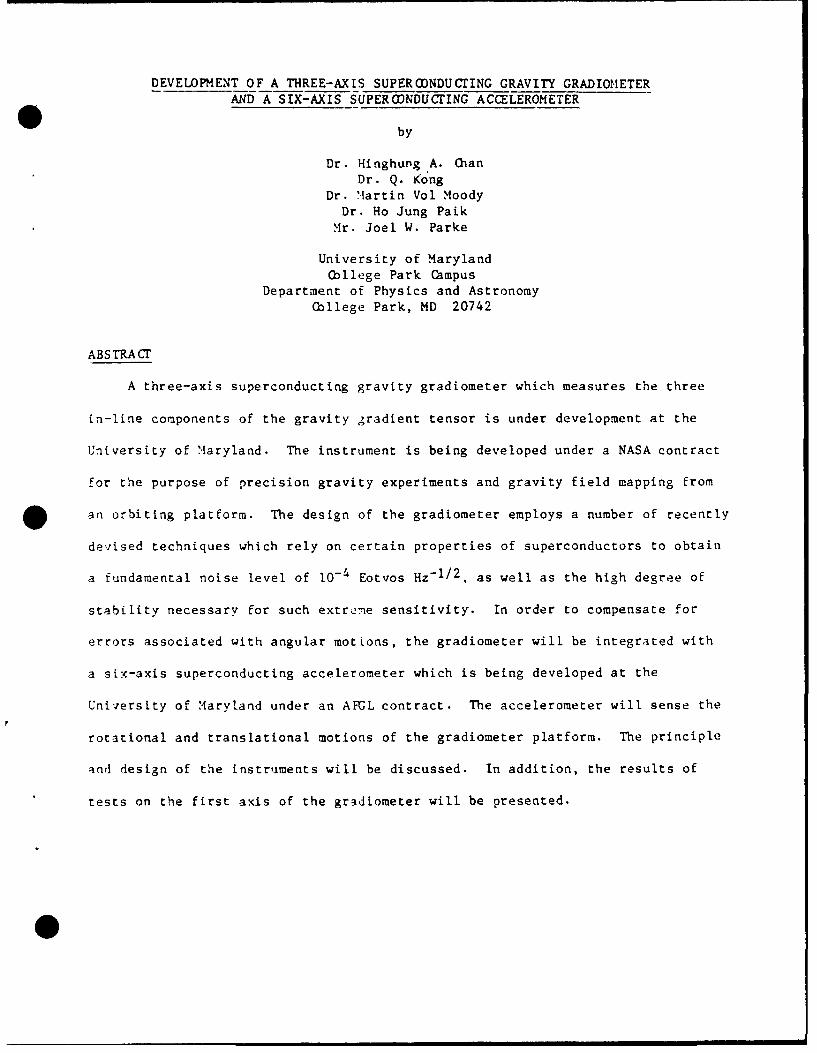
DEVELOPMENT OF A THREE-AXIS SUPERCONDUCTING GRAVITY GRADIOMETER

AND A SIX-AXIS SUPER()NDUCTING ACCELEROMETER

by

Dr. Hinghung A. ChanDr. Q. Kong

Dr. Martin Vol MoodyDr. Ho Jung Paik

Mr. Joel W. Parke

University of MarylandCollege Park Campus

Department of Physics and Astronomy

College Park, MD 20742

ABSTRACT

A three-axis superconducting gravity gradiometer which measures the three

in-line components of the gravity gradient tensor is under development at the

University of Maryland. The instrument is being developed under a NASA contract

for the purpose of precision gravity experiments and gravity field mapping from

an orbiting platform. The design of the gradiometer employs a number of recently

devised techniques which rely on certain properties of superconductors to obtain

a fundamental noise level of 10- 4 Eotvos Hz - I /2 , as well as the high degree of

stability necessary for such extreme sensitivity. In order to compensate for

errors associated with angular motions, the gradiometer will be integrated with

a six-axis superconducting accelerometer which is being developed at the

University of Maryland under an AFUL contract. The accelerometer will sense the

rotational and translational motions of the gradiometer platform. The principle

and design of the instruments will be discussed. In addition, the results of

tests on the first axis of the gradiometer will be presented.

-Devo/o,,,men/ ofa ThroeAx Saper-colnc/uclA 6Yrav,'I v~6-odeme/co'

/ca rA x is -,a rcfdaC4*An r~col/roo,re~or -.0

/Y A~ /A.C ~ha n, .//JIPz;k, alid W Parke"

S tepi. 0/Pf sc / al 'Y l5/4

s' 1 Oporred hy AFGL and "VSA conirccs

6~czr~meerPr,~ram

A~~/ 0~~ rO~~br /970 r -

fa Fr Vcr,n,? cfolo FeA I'757 - 19b i4ooP,

b)hpp ecri/r/e.b

0 M~

(n~ 0

z-Iz

zoI~z* -

cn z~U)

USA

3-AXIS SUPERCONDUCTING GRAVITY GRADIOMETERDESIGN FOR ONE OF SI:4 IDENTICAL UNITS

/0

EDMSLOTS

0

l 4 INCHES ..£COVER - XiIA I

COIL ,--"--SPRINGCOILS

JUNCTION __ __.PROOF

Box MASS

COIL HOUSINGFORMHOLDER L _

£

dale ai ?pe7o9se0

~~D (' , %rc ii'7 ® ner

Fn~r~-=tz4 kx' f cx ,'

CO.LS

COILS 3W50

COIL 35

340-

COILS

LE VITAT IONECOIL 310-

30 10 20 30 40 ~060 7M(Curm) 2

S/f) rIfkT E oMIZ t 2A,7 .

prodf maxiI

basc /'ne m

resonanice I/qetj<7q

L'emperca/ure .T t-fK

9ualI/J ac/or C10

amnpls/ie~r noise EAt/ -01#

e4Oer cvO1p/;/7 /'ar-ar *'

WflOU/ nejablve SPriri? I~ n e ave s)Or iny (~h

6olSolb Iq P3 wee-ks hol - 3 3x /0 e

CANTILEVER SPRING

n*eo $9 t r7

00oIo

I I

0 1

0 @

Sensing ci .reait -

a dj as ra/tO vi' I, fo 1, o balance oul

ornm on mode acce/erabion..

* Levi/a/ion circstd

2 LE

. inereafefc,,lf oersfolcft/ 'Y -2

I F-eeahacA-a, COld( W~,?Moi~nh6. f-orce reba/Qa.ec. hiyh frepuencyj rej c cl;on

i.Three dlimensioial ba/a,,ce

* Feed Lack Funcllolus

Force~ rchal/ance

IMainiain-i nll/ pvsshio ol proof' t71411Gs.Redaces 1704 nearilic-s.1ncrea~resr d9 nertva cs7.

Reoduce.r £2impl;1(4We d / igh 4irp r~c-co-

Prev'rd caj~io/;A, u-/od

0 M~~h tc~uc'4 c- -c 1 'an

Redu cers gjore,4.r ~o/rconce

Prim arj F rror- Source~s

Pezr / ia//l c4mcllo/cd 'b eOMMo4 M04 h4/an.17

Pers;ve rejee/Jon btpn/ &V

ertxoeirer.

Ce-nsj v 14i s a cra/, f~~

ir . -c

* ~ ~ ~~ny iA mo+t-o e tY r(foti(\

r"ACI ve oCan ,necosoe zccce2Wcn-s Infll

sc ~ c -reco

Or 3 ~er -ro (YaiCL)l'Izc .. ~ Mt) rnbe 62P

cc tt s0 (uct c c- ) ct~ Proo nmcss kSZ

. Cectk co'I anc L J~Scns( COt jri ~ y

IT- * ecc'il aC-e- m~n-'cObe

md\CSS.

Supercoiduc &ng St'X-ca's AcceIerorne+' r0

z

iy

Proof mass (Niobium) Coil form (Macor ceramic)(a) (b

Zly Zxy Sensing coil

2iy \Z xyLevitation coil

Coils (24 sensing coils + 24 levitation coils)

(c)

Ix rX INIPC IPC£

a , 000

13-C

IN I

iP

10

0x 0

Ihch

IN IN INt0

irnsoc t-la V7) 2 EA 0]

S4((h)-K.T r E4 /)

OaSi~p Pararcers

proof rncff aI kresonance foere i

amp/:ier rZO01ire EXOA~.71

elterg1 Coup /;n at- /ar -P

mon 'A& r/, Ii4ym

Accekrdi opta Al

(t PA ~ Y)M

tjo" 2 za'J

* LEVITATIOM CIRCU'IT

,Eqaoliollr of 1 1 on:

4)/,L 1 j2

/77 = ,r*7YCn P

04

A. 1 aslevi/a/ed,f- /0.( ~APOWER SPECI 8Avg 0%Ovlp Harnn

04 FE-__

Log 4Hag

rms____ _ _ _ _ _ _

V/CHz

Fxd ( 0 Hz 50

B. Bc//i malsses /eydialeo/ 1 L 7 APOWER SPECI BAvg _ %Ovl-p_ Han-n

Log ___

Mag

Hz 50z

A B

Log

Fxd X 0 HZ 50

Alo,/odinducianceo duof 4o0 supro/c /4f/k.

1tpool' miax

L __00__0_0___

F~rpand i~2 d orc'er

L-;0 hx A -L3 '- d1.

2,2

IIbN#6

om

-. ,p..

A.h

ACAM.

- :. -. -

r

I

nn

-40,.4c

CL C

TITLE OF PAPER: Development of A Three-Axis Superconducting Gravity Gradiometerand A Six-Axis Superconducting Accelerometer

SPEAKER: Martin Vol Moody

QUESTIONS AND COMMENTS:

1. Question: Charles F. Martin

The non-linear effects of levitation at 11.5 Hz caused by -d" and "D"dimensions can be ignored in space. Can you adjust adequately forsurface or near earth use?

Response:

Yes, that distance can be adjusted and should present no problem in nearearth operation.

2. Question: Anthony R. Barringer

Is the six axis accelerometer applicable in a I "g" environment?

Response:

Yes. tk plan to test it in a I "g" environment. It will levitate atI "g".

3. Question: James E. Fix

What Q (quality factor) did you achieve?

Response:

Q is pressure limited. Achieved Q = 105 in tests at Stanford.

THE GRAVITATIONAL MAGNETIC FIELD OF THE EARTH

AND THE POSSIBILITY OF MEASURING IT

USING AN ORBITING GRAVITY GRADIOMETER

by

Dr. 93hram Mashhoon

Department of Physics and Astronomy

University of Missouri-ColumbiaColumbia, MO 65211

ABS T RA Cr

Einstein's theory of gravitation predicts that a rotaring body such as the

Earth carries the local inertial frames around it ("dragging of the inertial

frames"). This results in an effective gravitational "magnetic" field due to

mass current in addition to the usual - i.e., essentially Newtonian - gravita-

tional "electric" field, in close analogy with the electromagnetic field around

a rotating charged body. This fundamental prediction of general relativity has

not yet been tested. A gravity gradiometer in Earth orbit measures mostly the

. components of the tidal field (i.e., curvature tensor) of the Earth. The

gravitational "electric" and "magnetic" fields of the Earth are reflected in

the tidal tensor. The tidal accelerations due to a rotating system have been

studied and the relativistic corrections to the Newtonian results have been

determined (Mashhoon and Theiss, Phys. Rev. Lett. 49, 1542-1545, 1982). The

possibility of measuring relativistic effects using Paik's superconducting

gravity gradiometer currently under development is irvestigated.

S

* ~ ~ ~ ~ ~ Aa nn1~ e~J ietryarc~z

HO H M(it",tier 0

E. Wed en 14Z £leetrogy,nao,,;c 7 ~ /

F. Hun d IV~f Cravdiaio'

s me0ry Pofa'' t.g/$ /1 xcess

DG37 or #Xe Lou/ 1.rhetla Far

pefe re,,cs T' M. F W. ~ I/4 Z) SX . 17 ls's 4u t Y ~ ,~ fg )

/,,,#4ed e',Z4e1 ?e vt1, Ver ?13eem ,*, ~W~ c.1

-- -o

~~An A

_rj

AA

-~J- -2.

-Q- =- & = -- [.z ,. :

-... 7r

S1

E -

OZerv),Le ek~. ~Iv~-c4s I

(vL) En~en'c.. Pin117 V4 elan~c

1',ert~P,l . = 11ta,4 M~ 4

Q-& I ~A~e 4 tclf~

A1,tr, ~ ~ d $ d lje,.,,, o&,6a1

r~2 (74 larVA)

* 4

2 x,( (t)

itz-71

21 , =0

I TIdA Matrix

6enercir eltvtt'-

jr- 2

f~~gE~din:+1 Z4U$~a k~~t~e/2.

Cfdzinc e.f. =0s

/evy~~~~ /?~I1R CkViar 7 ,

(i) CLmw. a. Ok t =t()

t r \( ) l.

2)

0) (()X

*V Anis7red et "l p

z L

Pt o . 0 x=0. t

1j) Mk MM(

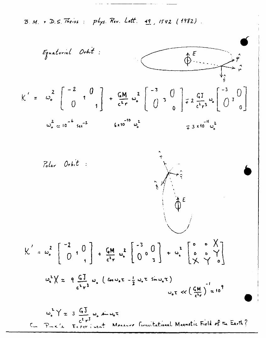
I'

__~~~ 0D X 2~ 43 02. -1.-1(L- 0

cj CV~o -CS WON

c -m f

3

r3 M ~~4i cF eK. -2 T

TITLE OF PAPER: The Gravitational Magnetic Field of the Earth and the Possibility

of Measuring it Using an Orbiting Gravity Gradiometer

O SPEAKER: Bahram Mashhoon

Q ESTIONS AND COMMENTS:

1. Question: Dan Long

Have the gravitational magnetic effects been derived classically as cani bedone in Electricity and Magnetism?

Response:

One would get about the same results but that theory has defects and I have

not used it.

2. Question: Alan Zorn

Your satellite examples show that the relativistic correction terms areboth conservative and harmonic (symmetric and traceless). Is this truein general?

Response:

Yes, general relativity implies this in general.

3. Question: Charles Finley

Does the orientation of the spacecraft, i.e., the orientation of the SCGwithin the Spacecraft (inertial vs. earth pointing) make a differencefor this experiment? If so, which would be preferred?

Response:

In theory, it would not matter which orientation were used since the

deviation from true gyroscopic inertial orientation would have to bemeasured and/or determined. However, in practice this is an importantquestion in that they would want the orientation to be such as to minimizethe difficulty in measuring the deviation from the true inertial.

4. Question: Warren Heller

What is the size of the quadrilateral/magnetic effect in ordinary terms?

Response:

3 x 10-11 of an orbit time.

TESTS OF GENERAL RELATIVITY IN EARTH ORBIT

USING A SUPERCONDUCTING GRAVITY GRADIOMETER

by

Dr. Ho Jung PaikDepartment of Physic. and Astronomy

University of MarylandCollege Park, MD 20742

ABSTRACT

A gravity gradiometer measures a component of the Riemann curvature tensor

which is the fundamental gravitational field in General Relativity. Both the

mass M and the angular momentum J of a spinning object contribute to the Riemann

tensor. For the Earth, the relativistic corrections due to M and J amount to

7 x 10-10 and 8 x 10-11 of the Newtonian gravity gradient, respectively. These

effects could be resolved with a signal-to-noise ratio of 10 in one year by a

three-axis superconducting gravity gradiometer of 10- 4 E Hz -1 / 2 sensitivity in a

* low-altitude polar orbit. We discuss the experimental strategy and the require-

ments that these experiments put on the orbit and the altitude control of the

spacecraft.

0

TESM- OF &E'NERAA REILqTVITr

SUPERCONDCTIN4r GAAVTY &KAbIOMETER

Ho 7a noi P4 or*beparme4f ef- P~ysfc4 o a4svnm

ver~PiP ' ryt4Id, 4 ff" ark

/o E~rtA OS~Srav;#/ FiW/f ;m, Crnm / /e4#j4'

z.Null 7TesiP o,' Emnsons PivE/S 1 N s

(5.ar~sA fie', ot rFyf th ree)

3.DefrAV Orwfe'0na uf "larehre. ",5elod

4/ /?PIJRP7.,"; *#,oc~ft n'0fdq4rve#

~# ~iIs ~r~ 4 Feld ?

w0~ Kepfci';a'ir3'

t:Proper A4,e

7741'pI4frgn (MahhoCD) Poltir Orbfl

3 0 / 4T ;rkcs.

rc'A X ,O 1

-f T2>1

sfedo i 1f r"

Mal n; Oi es

New4vm; a,7'rm

~I*OoE

( r\3 P1~ n6

(dc~~I

Re1q~~sco"ee4e~.2

(4 3gn TR~i'~~ 4 ac

r CIL

r'e 6 ime T 7rxEos

-V-A

ID

NbN

b 0

(?j-Z 3)Wzj )UAIIS3S N30z

8 y su*.lin;~; 9A^ vap I

3'

&Cclutfsce ' il

M~t, tes o# cror:

eNon. Or4*jc90141ioi &f Ire S..ms;$ve AXes

~) ~saf'D . tree SC4C usp*r4 In#ercigt~J of A xes

or wolimD"ilS *

E~o ~S~C~k *ftlpt X PO;n'*tV#?d

-3) CeifEi41 EACr4?'500,

WiA A-C Aid Pf SX-4AX;- 4(ce'Icpvnetet-

142

Source600

response to anpin1mss

**

Ylrt

zZIS

'4,auto

E 'Dl.

e. ,

Jxflverse5sirAa.'7s S

I ,

-2

0 3 _ STACY ,ViT /

107

_o _7 -1/--0 l I AR!Li

o o2 10 ' le I0 J6 1o7 1o8 IO9 1,o

RANGE OF FORCE 2k Cm)

. .. . -

3 e/'et~en of~ 6-rv;#hsvn4i "Maum7,e.4c" FelY

Oreet A.. I~rAgo*tr A~rfs 40

r _L A

of r + ro)

r-Ma 77C-1t

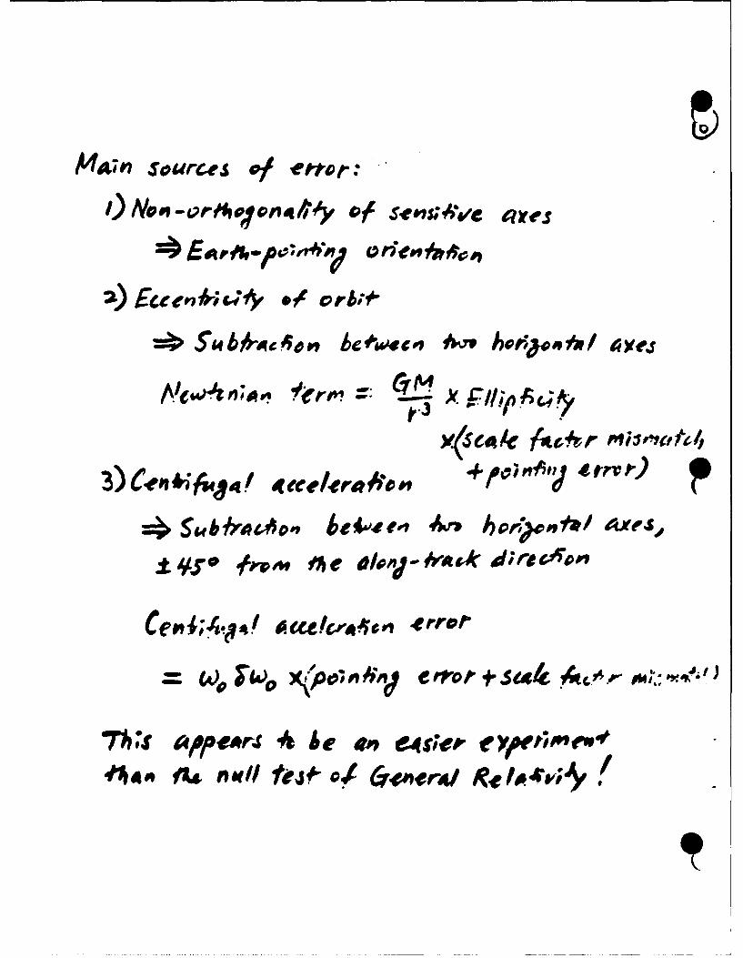
MAI-n sources Of e'rore:

/) Novo of#o4$~yG7 S el~ival ayc es

t-3

3)Cen,*tk~q! tteefera~m + 1001,

4j Ste b frp &Ap*7 be4oee-' 9I h&*i? 4xesJ,

±4#'* ,V 4e fak;w

= w, he e4ror * eafe Amew*

~ fL fle ?C#" 4CrPer4l ffl eif y

4 4

rl r

I' I.

vA 3

~rLr

tzt

ONOtoo

Lltoz

5 e If vejr'w~y OSr bit bE$a £ w or c.4op

:3) Sun-P sgcko"u~os Dri; tp

=EOS ? (Spook' I yr)

TITLE OF PAER: Tests of General Relativity in Earth Orbit Using A Superconducting

Gravity Gradiometer

SPEAKER: Ho Jung Paik

QLESTIONS AND LObLMENTS:

1. Question: Richard Hansen

What about interference to dragging of inertial frames from higher moments

of the earth?

Response:

These appear at higher multiples of the orbital frequency. The only effects

which can interfere are those with components at orbital frequency.

2. Question: Alan Zorn

Can you comment on the relationship between the current state of scale

factor mismatch that you expect on your current instrument and how the

requirements for null test (10-10) and magnetic field (10- 5 ) experiments can bemet?

Response:

We expect 10- 5 on the current 3-axis instrument, so the magnetic field

experiment can be done pretty easily. We recognize that the null test

experiment will be much harder. However, post processing of the data will

help us reach this goal, we believe.

MAGNETIC ISOLATION-CLOSING THE LOOP

0by

Dr. Dave Sonnabend

Mr. A. Miguel Fn Martin

Jet Propulsion Laboratory

California Institute of Technology

ABSTRACT

Progress on the design, construction, and testing of the JPL single axis

magnetic isolation test facility has been previously reported. Our more recent

work has been to close the loop with a digital computer, in order to try out

various vibration isolation and semi drag free control laws. The status of

this work will be reported. For vibration isolation, we will discuss both the

theoretical limitations of the technique, and the test limitations imposed by

the facility. Finally, for semi drag free operation, we will look at shaping

* of the current impulses, to minimize the excitation of vibration modes of the

floated instrument.

S

Magnetic Isolation-Closing the Loop

Dave Sonnabend and A. Miguel San Martin

Jet Propulsion Laboratory

California Institute of Technology

8 February 1987

Abstract

Progress on the design, construction, and testing of the JPL singleaxis magnetic isolation test facility has been previously reported. Ourmore recent work has been to close the loop with a digital computer,in order to try out various vibration and semi drag free control laws.The status of this work will be reported. For vibration isolation, we0 will discuss both the theoretical limitations of the technique, and thetest limitations imposed by the facility. Finally, for semi drag freeoperation, we will look at shaping of the current impulses, to minimizethe excitation of vibration modes of the floated instrument.

1 Introduction

Previous work on magnetic eddy current isolation of gradiometers was re-ported in Refs. 1 and 2. A single axis torsion pendulum facility was de-scribed, on which vibration isolation and semi drag free operation ideascould be tested. The facility characteristics, and initial testing of the mag-netic forcers was reported in Ref. 2. The abstract above tells what we wouldlike to have said today; but, as we have not made that much progress, I'lldiscuss only what we've actually accomplished. Mostly, this will cover ourefforts to close a digital control loop around the magnetic test facility. Atthe end I'll also mention some parallel analytical work, at Arizona StateUniversity, on the physics of eddy currents.

o1

0

2 Hardware Description

The plant (the original facility) comprises the torsion pendulum, four eddycurrent actuators, and two sensors. A photo, from Ref. 1, is shown in Fig. 1.The actuators are mounted externally, on brackets, positioned at oppositefaces of the box (where the gradiometer would reside), two on each side. Thecoil axes are normal to the box faces, along the direction of the box motion.The design and implementation of the torsion pendulum and actuators aredescribed in Ref. 2. A condensed theoretical treatment of eddy currentforcing is given in Ref. 1; and a substantial generalization in Ref. 3. Asynopsis of the latter work is presented here, in the final section.

The two sensors measure the displacement between the box and the brack-ets. They are Kaman Instrument Co. eddy current sensors, Model KD-2400.Each sensor consists of two subassemblies- the sensor head and a signal con-ditioning module. The proximity of the sensor to the box controls a variablegain oscillator within the conditioning module. The oscillator amplitude isdetected to provide an analog signal proportional to displacement. Amongthe sensor features are low cost, no contact, 10 kHz frequency response,adjustable gauge factor, and 0.25 mm resolution.

The function of the control loop is to execute a control law, designed toachieve certain performance objectives. The controller samples analog datafrom the sensors, converts these to digital form, computes actuator com-mands according to the trial control law. converts back to analog, and fi-nally doles out power to the actuators. All these operations are carriedout periodically, in real time. The two most important requirements of thishardware are at least 12 bit resolution, and a sampling frequency of at least10 Hz.

Fig. 2 shows the block diagram of the control loop. The computer is a PC'sLimited IBM AT compatible; and its characteristics are listed in Table 1.The function of the computer is to carry out the calculations dictated bythe control law, control the overall timing of the loop, and generate testevaluation data.

The :nput/output interface board is located in one of the expansion slots ofthe computer, and is connected to the computer output bus. Its function isto perform A/D and D/A input and output conversions. Table 2 lists thefunctions of the interface board. The board consists of a multiplexer, one

2

A/D and two D/A converters, a clock,---id a microprocessor that controlsthe operation of these elements and communicates with the computer mi-croprocessor in a high level command language. The analog outputs are ofthe sample and hold type. Purely digital input and output lines are alsoprovided.

The signal generator provides an analog sinusoidal constant amplitude andfrequency signal. We are presently operating at 40 kHz. The amplitudemodulator regulates the amplitude of the sinusoid according to the controlsignal from the interface board. At the time of the talk, this was a multiply-ing D/A converter (see Fig. 3); requiring a digital output from the interfaceboard. However, due to the unavailability of the DAC1220 micro-chip, thisapproach was changed to using an analog modulator, as shown in Fig. 4.

Finally, the function of the power amplifier is to amplify the signal from theamplitude modulator to provide the desired current to the forcing coils. Itis a standard stereo audio amplifier, a Phase Linear Model 400, Series Two.It can put out 205 watts rms into 8 f loads, and has a bandwidth of 50kHz. Since the talk, these loops have all been closed; and simple control

*laws have been demonstrated.

3 Eddy Current Analysis

In a parallel effort to achieve a better understanding of the physics of eddycurrent interactions, a contract was let to Arizona State University. Ear-Her work, summarized in Ref. 1, examined a conductive spherical shell onthe axis of a circular coil, carrying a sinusoidal current. The force anddissipation were calculated. The newer work, reported in Ref. 3, extendsthis to off-axis cases, and computes the torque on the sphere. The analyt-ical results are much too complicated to be presented here; however, thequalitative results are summarized in Fig. 5. As might be expected fromsymmetry considerations, the axial repelling force does not depend on dis-placement from the axis, to first order in this displacement; and there is notorque on-axis. However, off-axis, to first order in the displacement, thereis a force tending to restore the sphere to the axis, and a torque tending toroll the sphere toward the coil, both proportional to the displacement. Thedissipation in the sphere was shown not to vary, to first order in displace-ment. Future work is planned in this area to develop an electrical model of

3

the coil-sphere combination, that will serve as a basis for design of practicalisolation systems.

References

1) Seaman, C. H., and Sonnabend, D.; "Semi Drag Free Gravity Gradiom-etry"; J. Astron. Sci.; Vol. 33, No. 4; 1985.

2) Seaman, C. H., and Sonnabend, D.; "A Laboratory Single Axis MagneticIsolator"; JPL EM 343-1004; 3-21-86.

3) Bergman, J., and Hestenes, D.; "Eddy Currents in a Conducting Sphere";Dept. of Physics, Ariz. St. Univ. Final Report; 10-86; JPL No. 9950-1269.

4

LL.

<I < 1

L0

LLLU

-J LL-

F-F

<j-- =: :)V

_0 LUJ0 -. 0 <0 ~j=F- =3 ( -1< 0 0<D

<0 < CA ,L

<~ 0 LLJ - < ;7U0 F< (A0 <0 .. <<0< LLnC U ( _ LU~ cL V

w aa- = LU-

0>~ 0 = C)~LL/ Oem )u

CD C LU LC~

<~ C:) c- rL2J <<o<o<

< z F-LL-

Zj LU 0

f(A

C,,

(-

0 0

wU U- LUj

u < -J<0

M. 0in -

CA o < L -

LU 0 I

-J- =: L)Uz; 0I

LU<

L 0 L L -J

S< -LU)0CL O CD

P -i -~ C-) V) - - 0oLUCAC L < =D cm0

cn~~ ~ ~ ~ 0 LL Jc nU L L)

L 0 CAj B C. V) < a < <

0< Li- LU WA 0 < 0~0

z~~~V <<< U~ -

< < 0 U 10 %0 x >( xCL w~- C\ LU LUJ

L)LU

1LL

Il

.t

Fig. 1. Magnetic Isolation Test Facility

LU,

LUJ

-Y NLUi

LLJ

LUIU

C-)

LU~LLJ

LU.

< ) )iu 'wC

a..-0I

_ 0=

czz

==

a VI + 0

CA 1 +

_ 0 0 <c

< (D+

<- U L"

-~ 0 -JC)< ~ -

0 0 < .. -

ml 0Om>.LI C-4A

< 0 ~ >. 0 d

ii <

LUU

:;F L 0- L

0- LU <CA-

CIRCUIT SCHEMATIC

TYP4CAL MOOULATOPRiCUIT

Anlo Moulto

Figure 5.

EDDY CURRENT ANALYSIS

COIL SPHERE

Force: Zero Order - Away from CoilFirst Order - Toward Axis

Torque: Zero Order - NoneFirst Order - Roll Toward Coil

Dissipation: No First Order

I 5gg-2

0

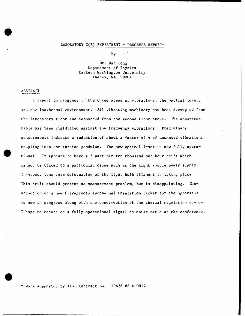
LABORATORY G(R) EXPERIMENT - PROGRESS REPORT*

by

Dr. Dan Long

Department of PhysicsEastern Washington University

Cheney, WA 99004

ABSTRACr

I report on progress in the three areas of vibrations, the optical lever,

ad the isothermal environment. All vibrating machinery has been decoupled from

the laboratory floor and supported from the second floor above. The apparatus

table has been rigidified against low frequency vibrations. Preliminary

measurements indicate a reduction of about a factor of 4 of unwanted vibrations

coupling into the torsion pendulum. The new optical lever is now fully opera-

* tional. It appears to have a 5 part per ten thousand per hour drift which

cannot be traced to a particular cause such as the light source power supply.

I suspect long term deformation of the light bulb filament is taking place.

This drift should present no measurement problem, but is disappointing. Con-

struction of a new (fireproof) isothermal insulation jacket for the apparatur'

is now in progress along with the construction of the thermal regulation devic..

I hope to report on a fully operational signal to noise ratio at the conference.

0* w ork upport,,d by Arn, . Contract No. F19628-86--K-0014.

LABORATORY G(R) EXPERIMENT - PROGRESS REPORT

February 1.987

DANIFl. R. LONG, Ph.DProfessor of Physics

Eastern~ Washington UniversityCheney, Washin~gton 99004

W.-rk supported by AFGL

Cont~ract No. F 19628-86-K-0014

I report on progress in overhauling and improving the

v.itern Washington University Cavendish Torsion Balance. Recent

improvements, mainly funded by AFGL, are illustrated in the

following slides presented at th' conference. These substantial

nodiffications addreised reducing the effects of tilt on the

output signal, reducing vibrations, and improving thermal

stability. The last illustration shows the gravitational force

signal now put out by the apparatus. It indicates about a 2 part

per ten thousand torque signal stability. This is about a factor

of t0 improvement over previous work.

0e

I%

View (1) The entire apparatus with ring masses in view. Note

the thin aluminum legs which are reinforced in the next picture.

6

!4

View (2) 3 x 3 x 1/2 aluminum angle has been used to reinforce

the frame. The 1/2" aluminum plate below the main table was

later loaded with 200 lbs of lead.

S Sht

View (3) A view of the frame showing the cross reinforcing.

View (4) A further view from the rear showing the cross

reinforcing.

j

View (5) The new, tilt proof, optical lever of quasi auto

collimator design can be seen in the right portion of the photo.

View (6) The new optLca. lever features a newly constructzed

external light source and fiber optics. This reduces temperature

dri!:~ in the~ vacuum chamber.

I

View (7) The fan for cooling the optical lever light source is

mounted on the I beams of the second floor above to provide

vibrational isolation. The 4 x 4 in the picture can exert a few

tons against the second floor to tilt the floor and apparatus at

will, without introducing further gravitational masses near the

* apparatus.

View (8) The newly constructed), thermally, and electrically

shielded output box for the opttcal lever.

View (9) The fore pump Is mnounted on 300 lbs of steel suspended

from the second floor above by chains. The vacuum hose goes to

500 lbs of scrap steel which markedly reduces vibrations.

p

View (10) After leaving the 500 Ibs inertial block mass, the

fore-line hose goes to a 400 lbs mass mounted on lead bricks.

I

View (11) The newly constructed isothermal water bath needed to

supply the diffusion pump with constant temperature water has

several vibrating components. These are mounted on the angle

Iron seen hanging down.

S

View (12) The water bath angle iron proceeds through the ceiling

to the second floor I beams above.

9

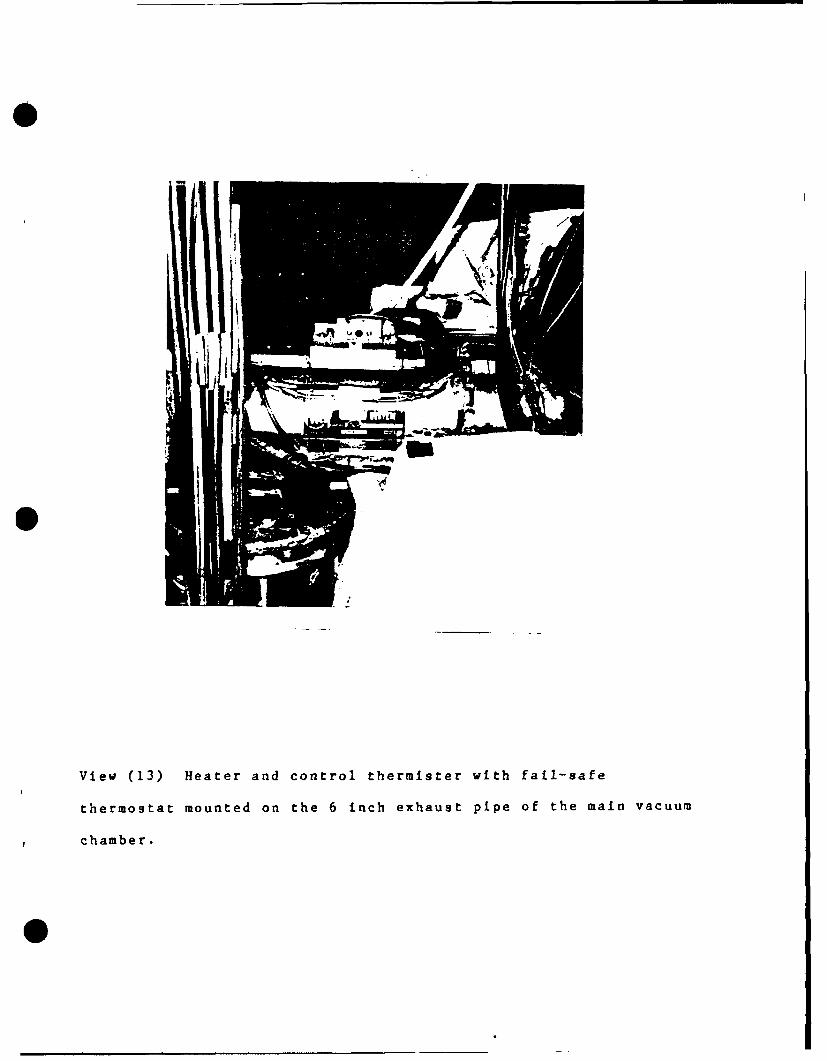
SA

View (13) Heater and control thermister with fail-safe

thermostat mounted on the 6 inch exhaust pipe of the main vacuum

chamber.

A66

View (14) Heater and control thermister with fail-safe

thermostat mounted on the North-East leg.

View (15) Heater and control thermister with fail safe

thermostat mounted on the West leg.

...... ......

!0

" " 000 °

View (16) The five 0.01 C Yellow Springs Instrument Company

thermal controllers used to control power to the heaters.

View (17) Newly constructed, fire proof, fitser glass fabric and

fitser glass felled insulation.

ijqMI i:

View (18) Insulation of the sphere top. An additional 6 inch

hood covers what is seen. Preliminary results suggest 0-0010C

stability over a few hours.

View (19) A thermister shown on the side of the attracted ball

chamber. This thermister will monitor any changes in temperature

produced by introducing the attracting masses near the chamber.

18 thermisters hive been mounted on the apparatus.

A I I VH

I eni

View (20) Strip chart trace of the optical lever )utput of the

gravitational signal. 10 intervals is 1% of the ring torque

signal. The centroid of the sine wave seems stable to 2 or 3

parts per ten thousand of the ring torque.