Load Data Analysis User Guide Release 1.11.1.3 for Windows
434
Oracle Utilities Load Analysis Load Data Analysis User Guide Release 1.11.1.3 for Windows E18229-11 September 2020
Transcript of Load Data Analysis User Guide Release 1.11.1.3 for Windows
Oracle Utilities Load AnalysisLoad Data Analysis User GuideRelease 1.11.1.3 for WindowsE18229-11
September 2020

Oracle Utilities Load Analysis Load Data Analysis User’s Guide, Release 1.11.1.3 for Windows
E18229-11
Copyright © 1999, 2020 Oracle and/or its affiliates. All rights reserved.
This software and related documentation are provided under a license agreement containing restrictions on use and disclosure and are protected by intellectual property laws. Except as expressly permitted in your license agreement or allowed by law, you may not use, copy, reproduce, translate, broadcast, modify, license, transmit, distribute, exhibit, perform, publish, or display any part, in any form, or by any means. Reverse engineering, disassembly, or decompilation of this software, unless required by law for interoperability, is prohibited.
The information contained herein is subject to change without notice and is not warranted to be error-free. If you find any errors, please report them to us in writing.
If this is software or related documentation that is delivered to the U.S. Government or anyone licensing it on behalf of the U.S. Government, the following notice is applicable:
U.S. GOVERNMENT END USERS: Oracle programs, including any operating system, integrated software, any programs installed on the hardware, and/or documentation, delivered to U.S. Government end users are “commercial computer software” pursuant to the applicable Federal Acquisition Regulation and agency-specific supplemental regulations. As such, use, duplication, disclosure, modification, and adaptation of the programs, including any operating system, integrated software, any programs installed on the hardware, and/or documentation, shall be subject to license terms and license restrictions applicable to the programs. No other rights are granted to the U.S. Government.
This software or hardware is developed for general use in a variety of information management applications. It is not developed or intended for use in any inherently dangerous applications, including applications that may create a risk of personal injury. If you use this software or hardware in dangerous applications, then you shall be responsible to take all appropriate fail-safe, backup, redundancy, and other measures to ensure its safe use. Oracle Corporation and its affiliates disclaim any liability for any damages caused by use of this software or hardware in dangerous applications.
Oracle and Java are registered trademarks of Oracle and/or its affiliates. Other names may be trademarks of their respective owners.
Intel and Intel Xeon are trademarks or registered trademarks of Intel Corporation. All SPARC trademarks are used under license and are trademarks or registered trademarks of SPARC International, Inc. AMD, Opteron, the AMD logo, and the AMD Opteron logo are trademarks or registered trademarks of Advanced Micro Devices. UNIX is a registered trademark of The Open Group.
This software or hardware and documentation may provide access to or information on content, products, and services from third parties. Oracle Corporation and its affiliates are not responsible for and expressly disclaim all warranties of any kind with respect to third-party content, products, and services. Oracle Corporation and its affiliates will not be responsible for any loss, costs, or damages incurred due to your access to or use of third-party content, products, or services.
ContentsIntroduction
Is This Guide for You?.................................................................................................................................................... i-iHow To Use This Guide................................................................................................................................................. i-iWhat You Should Know Before Getting Started........................................................................................................ i-iConventions Used in This Guide ................................................................................................................................. i-iiOther Load Analysis Documentation ......................................................................................................................... i-iiiHow To Get Help .......................................................................................................................................................... i-iii
Chapter 1Load Research and the Oracle Utilities Load Analysis System ........................................................................ 1-1
What Is Load Research? ................................................................................................................................................ 1-2How Do Utilities Conduct Load Research?............................................................................................................... 1-4What Does Oracle Utilities Load Analysis Do? ........................................................................................................ 1-5
Chapter 2Overview of the Oracle Utilities Load Data Analysis System .......................................................................... 2-1
What Is the Purpose of the Load Data Analysis System?........................................................................................ 2-2How Does It Work?....................................................................................................................................................... 2-3How Is the LAS Structured?......................................................................................................................................... 2-9Working With the Load Data Analysis Subsystem — What Steps Do You Follow? ....................................... 2-10
Step 1: Inputting Data ................................................................................................................................. 2-10Step 2: Modifying Data ............................................................................................................................... 2-10Step 3: Analysis — Expanding Data to Class Level Estimates............................................................. 2-11Step 4: Analysis — Aggregating Class Estimates to the System Level ................................................ 2-11Step 5: Reporting.......................................................................................................................................... 2-11Step 6: Additional Analysis ......................................................................................................................... 2-11Step 7: Archiving Statistics and Load Data.............................................................................................. 2-12
Chapter 3The Oracle Utilities Load Analysis Data Formats ........................................................................................... 3-1
ELDB Load Data Records ........................................................................................................................................... 3-2Cuts, Cut Series, and Cut Keys .................................................................................................................... 3-2Header and Interval Data in Load Data Records ..................................................................................... 3-4Record Types and Flags ................................................................................................................................ 3-8
Statistics Records ............................................................................................................................................................ 3-8Statistics Identifiers........................................................................................................................................ 3-8Header and Interval Data for Statistics Records..................................................................................... 3-10
Chapter 4Oracle Utilities Load Analysis Mechanics........................................................................................................ 4-1
What Input Files are Used in Oracle Utilities Load Analysis? ................................................................................ 4-2What Output Files Does Oracle Utilities Load Analysis Produce? ........................................................................ 4-2Naming Conventions in Oracle Utilities Load Analysis........................................................................................... 4-3Using the Key Generator Preprocessor in a Control File........................................................................................ 4-4
i
ii
Preprocessing Options .................................................................................................................................. 4-4Supported Programs...................................................................................................................................... 4-5
Querying the Database with Embedded Query Statements .................................................................................... 4-7Syntax for Embedded Query Statements ................................................................................................... 4-7Supported Programs.................................................................................................................................... 4-11Custom Variables ......................................................................................................................................... 4-12
Chapter 5Getting Data into the Extracted Load Database (Y130, Y220, Y240)............................................................... 5-1
What Does ALDB/CLDB/ELDB Extraction Do?................................................................................................. 5-2Deciding Whether to Extract Data from the ALDB, CLDB or ELDB................................................................ 5-3Establishing Guidelines for Data Extraction ............................................................................................................. 5-3Record Flags and Validation Tests — Oracle Utilities Load Analysis “Quality Control” Mechanisms........... 5-4Steps for Using the ALDB/CLDB/ELDB Extraction Program (Y240).............................................................. 5-5Step 1: Create the Load Data Extraction Environment File (TGY24B.ENV) .................................................... 5-6
Step 2: Create the Load Data Extraction Control File (TGY24A.CTL)............................................... 5-8Step 3: Run ALDB/CLDB/ELDB Extraction Program (Y240)........................................................... 5-8ALDB/CLDB/ELDB Extraction Program (Y240) ................................................................................ 5-8
Chapter 6Modifying Customer Load Data Prior to Analysis Using the ELDB Load Data Editor (Y630) ..................... 6-1
Overview.......................................................................................................................................................................... 6-2Using the Load Data Reporter to Examine Cuts ...................................................................................................... 6-3Steps for Using the ELDB Load Data Editor (Y630) .............................................................................................. 6-3
Step 1: Create the Editor Control File Containing your Edit Commands............................................ 6-3ELDB Edit Command Summary ................................................................................................................ 6-4Guidelines for Using the Edit Commands................................................................................................. 6-6Step 2: Run the ELDB Load Data Editor Procedure (Y630) ................................................................. 6-7
Chapter 7Expanding Load Data to Class-Level Estimates Using the Load Analysis Programs (Y310 and Y330)......... 7-1
Comparison of MPU and Ratio Analysis Methodologies ........................................................................................ 7-2Three Methods of Ratio Estimating............................................................................................................................ 7-3Preparing for Analysis.................................................................................................................................................... 7-3Steps for Using the Standard Load Analysis or Ratio Analysis Procedures (Y310 or Y330) ............................. 7-5
Step 1: Ensure that Customer Load Data for the entire Analysis Period is Available ........................ 7-6Step 2: Create the Analysis Control File (TGY31A.CTL or TGY33A.CTL)....................................... 7-7Step 3: Create the Analysis Environment File (TGY31B.ENV or TGY33B.ENV)........................... 7-8Step 4: Modify the Time-of-Use File (TGY31D.TOU) if necessary ................................................... 7-18Step 5: Modify the Season File (TGY31E.SEA) if Necessary .............................................................. 7-20Step 6: Modify the User-Specified Day File (TGY31F.USD) if Necessary ........................................ 7-22Step 7: Verify the Holiday File (TGY31C.HOL) Set Up....................................................................... 7-23Step 8: Run the Standard Load Analysis Program (Y310 or Y330) ..................................................... 7-24Bias Tests — Ratio Only ............................................................................................................................ 7-27Step 9: Check Output .................................................................................................................................. 7-28
Chapter 8Computing Statistics for 100% Sampled Populations (Y380)........................................................................... 8-1
What Does the 100% Sample Analysis Program Do?.............................................................................................. 8-2Steps for Using the 100% Sample Analysis Program (Y380) .................................................................................. 8-2
Step 1: Ensure the tableset (CLDB or ELDB) contains Load Data for all customers. ...................... 8-3Step 2: Create the Analysis Control File (TGY38A.CTL) ....................................................................... 8-4Step 3: Create the Analysis Environment File (TGY38B.ENV) ............................................................ 8-5Step 4: Verify or modify other Required Input Files.............................................................................. 8-10Step 5: Run the 100% Sample Analysis Program (Y380) ...................................................................... 8-10
Chapter 9
Expanding Class Level Estimates to the System Level Using the Aggregate Load Analysis Program (Y320) 9-1
What Does the Aggregate Load Analysis Program Do? .......................................................................................... 9-2Steps for Using the Aggregate Load Analysis Program (Y320) .............................................................................. 9-3
Step 1: Ensure the Statistics you Aggregate are Available in the ELDB............................................... 9-3Step 2: Create the Aggregate Load Analysis Control File (TGY32A) ................................................... 9-3Step 3: Create the Aggregate Load Analysis Environment File (TGY32B) ......................................... 9-6Step 4: Run the Aggregate Load Analysis Program (Y320)..................................................................... 9-9Aggregate Analysis Processing..................................................................................................................... 9-9
Chapter 10Estimating Average Peak Load Using the Coincident Peak Analysis Program (Y340) ................................. 10-1
What Does the Coincident Peak Analysis Program Do? ....................................................................................... 10-2Steps for Using the Coincident Peak Analysis Program (Y340) ........................................................................... 10-3
Step 1: Ensure Data You Analyze is Available in Either the ALDB or the ELDB .......................... 10-4Step 2: Create the Coincident Peak Analysis Control File (TGY34A.CTL)....................................... 10-4Step 3: Create the Coincident Peak Analysis Environment File (TGY34B.ENV)............................ 10-7Step 4: Run the Coincident Peak Analysis Program (Y340)................................................................ 10-11
Chapter 11Estimating Loads for Subpopulations Using the Domains Analysis Programs (Y350 or Y360) .................... 11-1
The Domains Analysis Programs............................................................................................................................... 11-2Expansion Methods..................................................................................................................................... 11-2Results............................................................................................................................................................ 11-2
Steps for Using the Domains Analysis Program (Y350 or Y360) ........................................................................ 11-3Step 1: Ensure Data is Available in the ELDB ....................................................................................... 11-4Step 2: Create the Analysis Control File (TGY35A.CTL or TGY36A.CTL)..................................... 11-4Step 3: Create the Analysis Environment File (TGY35B.ENV or TGY36B.ENV)......................... 11-7Step 4: Verify or Modify Other Required Input Files .......................................................................... 11-17Step 5: Run the Analysis Program........................................................................................................... 11-17Domains Analysis Mean Per Unit Processing ....................................................................................... 11-17Domains Analysis Ratio Processing........................................................................................................ 11-19Bias Tests..................................................................................................................................................... 11-22Step 6: Check Output ................................................................................................................................ 11-22
Chapter 12Reporting Statistics and Load Data (Y410 - Y460) .......................................................................................... 12-1
Time Series Reporter (Y410) ...................................................................................................................................... 12-2Steps for Using the Time Series Reporter................................................................................................ 12-3Step 1: Create the Time Series Reporter Environment File (TGY41B.ENV) ................................... 12-3Step 2: Create the Time Series Reporter Control File (TGY41A.CTL) .............................................. 12-4Heading Commands .................................................................................................................................... 12-4Key Commands............................................................................................................................................ 12-5Step 3: Run the Time Series Reporter Program (Y410)......................................................................... 12-7Time Series Reporting Processing............................................................................................................. 12-7
Load Data Reporter (Y420, Y430)............................................................................................................................. 12-7Steps for Using the Load Data Reporter.................................................................................................. 12-8Step 1: Identify Records to be Reported and Type of Report Needed for Each One ..................... 12-8Step 2: Create Environment File (TGX41B.ENV) ................................................................................ 12-8Step 3: Create Control File (TGX41A.CTL) ......................................................................................... 12-13Step 4: Run the Load Data Reporter (Y420 or Y430).......................................................................... 12-14Load Data Reporter Processing............................................................................................................... 12-14
The Summary Reporter (Y440, Y460) .................................................................................................................... 12-15Steps for Using the Summary Reporters ................................................................................................ 12-16Step 1: Create the Control File (TGY44A.CTL) to Select Specific Cuts for Reporting ................. 12-16Step 2: To report cuts within a date range create the Environment File (TGY44B.ENV)............ 12-16
iii
iv
Step 3: Run the Summary Reporter ........................................................................................................ 12-17SLDB Summary Reporter Processing..................................................................................................... 12-17
Chapter 13Computing Customer Energy Use by Billing Cycles Using the Billed Energy Program (Y230)................... 13-1
Why Accurate Energy for Billing Periods Is Important to Ratio Analysis.......................................................... 13-2What Does the Billed Energy Program Do?............................................................................................................ 13-2Steps for Using the Billed Energy Program (Y230) ................................................................................................ 13-3
Step 1: Ensure Interval data used for computing Billed Energy is available in the ELDB.............. 13-3Step 2: Create the Billed Energy Control File (TGY23A.CTL)............................................................ 13-3Step 3: Create the Billed Energy Cycle File (TGY23X.CYC) ............................................................... 13-7Step 4: Create the Billed Energy Environment File (TGY23B.ENV)................................................. 13-8Step 5: Run the Billed Energy Program (Y230) .................................................................................... 13-10Billed Energy Program Processing.......................................................................................................... 13-10
Chapter 14Key Generators — Shortcuts for Creating Input Files and Reports................................................................ 14-1
What Is the Purpose of Key Generators?................................................................................................................. 14-2Introducing the Control Language ............................................................................................................................ 14-3Control Language — Logic and Structure ............................................................................................................... 14-3
Test Statements ............................................................................................................................................ 14-5Some Tips on Constructing Test Statements .......................................................................................... 14-8Format Statements..................................................................................................................................... 14-10SUBSTR Functions.................................................................................................................................... 14-11Counter Variables ...................................................................................................................................... 14-12
A Checklist for Using the Control Language......................................................................................................... 14-13Sample Control Files for Key Generators .............................................................................................................. 14-14
Example #1 — CLDB Key Generator Control File ........................................................................... 14-14Example #2 — CLDB Key Generator Control File ........................................................................... 14-15Example #3 — CLDB Key Generator Control File ........................................................................... 14-16Example #4 — CLDB Key Generator Control File ........................................................................... 14-16Example #5 — ALDB Key Generator Control File ........................................................................... 14-17Example #6 — ALDB Key Generator Control File ........................................................................... 14-18Example #7 — ELDB Key Generator Control File ........................................................................... 14-19Example #8 — ELDB Key Generator Control File ........................................................................... 14-19Example #9 — SLDB Key Generator Control File ............................................................................ 14-19Example #10 — SLDB Key Generator Control File .......................................................................... 14-20
Using the Key Generator Programs ........................................................................................................................ 14-20Step 1: Create the Key Generator Control File (TGX81A.CTL, TGX82A.CTL, TGY81A.CTL,
TGY82A.CTL) ............................................................................................................................................................................ 14-20Step 2: Add the (optional) Environment File ........................................................................................ 14-20Step 3: Run the Key Generator Program............................................................................................... 14-22Key Generator Processing........................................................................................................................ 14-22Step 4: Check Output ................................................................................................................................ 14-22
Chapter 15Performing Ad Hoc Load Calculations Using the Transformation Program (X620, Y620) ........................... 15-1
What Does the Transformation Program Do?........................................................................................................ 15-2Using the Transformation Commands ..................................................................................................................... 15-2
Constructing Blocks .................................................................................................................................... 15-2Using Variables............................................................................................................................................. 15-2One Type of Transformation Command — Arithmetic Operations.................................................. 15-3Another Type of Transformation Command — Transformation Functions .................................... 15-5
Steps for Using the Transformation Program ....................................................................................................... 15-14Step 1: Create the Transformation Environment File (TGY62B.ENV)........................................... 15-15Step 2: Create the Transformation Control File (TGY62A.CTL)...................................................... 15-17
Step 3: Run the Transformation Program.............................................................................................. 15-17Transformation Processing ...................................................................................................................... 15-17
Chapter 16Making Oracle Utilities Load Analysis Data Available for External Applications (X710, Y710, X720, X740, Y720, Y740, Y780)....................................................................................................................................................... 16-1
Direct Output Program ............................................................................................................................................... 16-3Steps for Using the Direct Output Program............................................................................................................ 16-4
Step 1: Verify that the Data you wish to Output is in the Source Tableset(s).................................... 16-5Step 2: Create the Direct Output Control File ........................................................................................ 16-5Step 3: Create the Direct Output Environment File .............................................................................. 16-6Step 4: Run the Program (Y720) ............................................................................................................. 16-11Direct Output Processing ......................................................................................................................... 16-12
The Direct Output Format (.INP)........................................................................................................................... 16-13Standard Format......................................................................................................................................... 16-13
Daily Output Format ................................................................................................................................................. 16-15Character Daily Energy Format............................................................................................................... 16-15
Statistical Package Interface Program (X710, Y710) ............................................................................................ 16-16Steps for Using the Statistical Package Interface Program (X710, Y710) ......................................................... 16-16
Step 1: Verify that the Data you wish to Output is in the Source Database(s) ................................ 16-17Step 2: Create the Statistical Package Interface Control File (TGY71A.CTL)................................. 16-17Step 3: Create the Statistical Package Interface Environment File (TGY71B.ENV)...................... 16-18Step 4: Run the Program (X710, Y710).................................................................................................. 16-19Statistical Package Interface Processing ................................................................................................. 16-19Step 5: Check Output ................................................................................................................................ 16-20
Statistic Extraction Program (Y780)........................................................................................................................ 16-22Steps for Using the Statistic Extraction Program (Y780) .................................................................................... 16-22
Step 1: Verify that the Data you wish to Output is in the Source Tableset(s).................................. 16-23Step 2: Create the Statistic Extraction Control File.............................................................................. 16-23Step 3: Create the Statistic Extraction Environment File.................................................................... 16-25Step 4: Run the Program (Y780) ............................................................................................................. 16-28Statistic Extraction Processing................................................................................................................. 16-29Step 5: Check Output ................................................................................................................................ 16-29
Chapter 17Housekeeping (Y910 and Y960)....................................................................................................................... 17-1
Steps for Using the Archive/Delete Program (Y910) ............................................................................................ 17-3Step 1: Create Key Generator (TGY11A.CTL) or Archive/Delete Control File (TGX92A.CTL) 17-3Step 2: Run Archive/Delete (Y910).......................................................................................................... 17-4Archive/Delete Processing......................................................................................................................... 17-4Step 3: Check and KEEP Output ............................................................................................................. 17-4Step 4: ELDB Recovery (If Malfunction Occurs) .................................................................................. 17-4
Steps for Using the SLDB Retrieval Program (Y960) ............................................................................................ 17-5Step 1: Create the Retrieval Control File (TGX66A.CTL).................................................................... 17-5Step 2: Create the Retrieval Environment File (TGX66B.ENV)......................................................... 17-6Step 3: Run the SLDB Retrieval Program................................................................................................ 17-7Retrieval Processing..................................................................................................................................... 17-7
Chapter 18The Cut Series Gap Report Program(Y490 - Y491) .................................................................................................................................................... 18-1
Steps for Using the Cut Series Gap Report Program ............................................................................................. 18-2Step 1: Create the Control File to Select Specific Cuts for Reporting................................................. 18-2For Load Data Records............................................................................................................................... 18-2Step 2: Create the Environment File......................................................................................................... 18-3Step 3: Run the Cut Series Gap Report Program ................................................................................... 18-4
v
vi
SLDB Summary Reporter Processing....................................................................................................... 18-4
Chapter 19The Daytype Analysis Program (Y760 — Y770).............................................................................................. 19-1
Input Preparation ......................................................................................................................................................... 19-2Control File (TGY76A.CTL) ..................................................................................................................... 19-2Environment File (TGY76B.ENV) .......................................................................................................... 19-3Peak Days File (TGY76C.PEA) ................................................................................................................ 19-4Holiday File (TGY31C.HOL).................................................................................................................... 19-5Season File (TGY31E.SEA)....................................................................................................................... 19-5
Processing Summary .................................................................................................................................................... 19-5Summary of Outputs ................................................................................................................................................... 19-5
Daytype File (TGY761) .............................................................................................................................. 19-6
Chapter 20The Individual Customer Analysis Program ................................................................................................... 20-1
What Additional Capabilities Does ICA Provide? .................................................................................................. 20-2What Can the Individual Customer Analysis Program Do? .................................................................................. 20-3Analysis Options........................................................................................................................................................... 20-4Reporting ....................................................................................................................................................................... 20-6Saving the Statistics for Further Analysis ................................................................................................................. 20-6Steps for Using the Individual Customer Analysis Program ................................................................................. 20-6
Step 1: Create the Analysis Control File (TGY37A.CTL) ..................................................................... 20-8Step 2: Create the Analysis Environment File (TGY37B.ENV) ........................................................ 20-10Step 3: Modify the Time-of-Use Schedule and Season Files if Necessary........................................ 20-15Step 4: Modify the Billing Cycle File (TGY23E.CYC) if necessary ................................................... 20-15Step 5: Modify the Demand Period File (TGY37E.DEM) if Necessary .......................................... 20-16Step 6: Verify that the Holiday File (TGY31C) has Been Set Up Properly ...................................... 20-18Step 7: Run the Individual Customer Analysis Program ..................................................................... 20-18Step 8: Check Output ................................................................................................................................ 20-18
Sample Applications of the Individual Customer Analysis Program ................................................................. 20-19Example A — Non-Contiguous Periods................................................................................................................ 20-20Example B — CLDB Cuts ....................................................................................................................................... 20-21Example C — Curtailment Periods......................................................................................................................... 20-22Example D — TOU Periods.................................................................................................................................... 20-23Individual Customer Analysis Statistics Output File Format .............................................................................. 20-24File Formats ................................................................................................................................................................ 20-24Quick Reference ......................................................................................................................................................... 20-29
Individual Customer Analysis Program Numbers ................................................................................ 20-29Control File Record Format..................................................................................................................... 20-29Environment File Record Format........................................................................................................... 20-29Average Day Type Statistics Abbreviations ........................................................................................... 20-30Demand Period File Record Format ...................................................................................................... 20-30Time-Of-Use Schedule File Record Format.......................................................................................... 20-30Holiday File Record Format..................................................................................................................... 20-30Oracle Utilities Load Analysis Status Codes .......................................................................................... 20-31
Chapter 21Oracle Utilities Load Analysis Proxy Day Selection Program (X670)............................................................. 21-1
What Does The Proxy Day Selection Program Do? .............................................................................................. 21-2Eligibility Testing.......................................................................................................................................................... 21-2Ranking of Eligible Days............................................................................................................................................. 21-3
Magnitude...................................................................................................................................................... 21-3Shape.............................................................................................................................................................. 21-3
Creating the Environment File (TGX67B) .............................................................................................................. 21-4Program Outputs.......................................................................................................................................................... 21-8
Proxy Day Return Codes............................................................................................................................................. 21-9Proxy Day Return Code List ...................................................................................................................................... 21-9
Appendix AGlossary of Load Research Terms.................................................................................................................... A-1
Appendix BAnalysis Equations ........................................................................................................................................... B-1
Load Analysis Programs............................................................................................................................................... B-1B.1 Non-Stratified Std. Load Analysis Equations (Mean-per-Unit) ..................................................... B-1B.2 Stratified Standard Load Analysis Equations (Mean-per-Unit) ...................................................... B-2B.3 100% Sample Analysis Equations (No Expansion).......................................................................... B-3B.4 Aggregate Load Analysis Equations (Combining Only Sampled Classes).................................... B-4B.5 Aggregate Load Analysis Equations (Combining Sampled and 100% Classes)........................... B-5B.6 Average Day Statistics ........................................................................................................................... B-5
Appendix CRatio Analysis Equations.................................................................................................................................. C-1
C.1 Non-Stratified Ratio Analysis Equations............................................................................................................ C-2Required Conditions for the Correct Application of Ratio Estimation ............................................... C-4
C.2 Separate (Stratified) Ratio Analysis Equations................................................................................................... C-5Required Conditions for the Correct Application of Ratio Estimation ............................................... C-8
C.3 Combined (Stratified) Ratio Analysis Equations............................................................................................... C-9Required Conditions for the Correct Application of Ratio Estimation ............................................. C-11
Average Day Statistics................................................................................................................................................. C-12
Appendix DReading “Analysis Statistics Written to the ELDB” Reports and Listings of Analysis Statistic Names....... D-1
How to Read the “Analysis Statistics Written to the ELDB” Reports ................................................................ D-2
Appendix EIndividual Customer Statistics File Formats ................................................................................................... E-1
Standard Load Analysis (Y310) ................................................................................................................................... E-1Ratio Analysis (Y330).................................................................................................................................................... E-1Domains MPU (Y350).................................................................................................................................................. E-1Domains Ratio (Y360).................................................................................................................................................. E-2100% Sample Analysis (Y380)..................................................................................................................................... E-2
Appendix FCoincident Peak Analysis Equations................................................................................................................ F-1
F.1 Non-Stratified Coincident Peak Analysis Equations (Mean-Per-Unit) .......................................................... F-1Average Customer Level.............................................................................................................................. F-2Customer Class Level ................................................................................................................................... F-3
F.2 Non-Stratified Coincident Peak Analysis Equations (Ratio) ........................................................................... F-5Average Customer Level.............................................................................................................................. F-5Customer Class Level ................................................................................................................................... F-7
F.3 Stratified Concident Peak Analysis Equations (Mean-Per-Unit)................................................................... F-10Average Customer Level............................................................................................................................ F-10Customer Class Level ................................................................................................................................. F-12
F.4 Stratified Coincident Peak Analysis Equations (Combined Ratio) ............................................................... F-14Average Customer Level............................................................................................................................ F-14Customer Class Level ................................................................................................................................. F-17
Appendix GDomains Analysis Ratio Equations................................................................................................................. G-1
Non-Stratified Domains Analysis Ratio Equations ................................................................................................ G-1Combined (Stratified) Ratio Analysis Equations ..................................................................................................... G-6Required Conditions for the Correct Application of Domains Ratio Estimation ........................................... G-10
vii
viii
Average Day Statistics................................................................................................................................................ G-10
Appendix HDomains Analysis Mean Per Unit Equations.................................................................................................. H-1
G.1 Non-Stratified Domains Analysis Mean-Per-Unit Equa ........................................................................tions H-2G.2 Stratified Domains Analysis Mean-Per-Unit Equations .................................................................................. H-4Average Day Statistics................................................................................................................................................... H-6
Appendix IDomains Analysis Ratio Equations................................................................................................................... I-1
H.1 Non-Stratified Domains Analysis Ratio Equations........................................................................................... I-1Required Conditions for the Correct Application of Domains Ratio Estimation............................... I-5
H.2 Combined (Stratified) Domains Analysis Ratio Equations.............................................................................. I-6Required Conditions for the Correct Application of Domains Ratio Estimation............................... I-9
H.3 Average Day Statistics.......................................................................................................................................... I-10
Appendix JOracle Utilities Unit of Measure Codes............................................................................................................. J-1
Appendix KKey Generator Variable Lists ............................................................................................................................ K-1
Index

IntroductionIs This Guide for You?
The Oracle Utilities Load Data Management and Analysis System is a comprehensive software tool designed to help utilities collect, manage, and analyze reliable load research data.
The Oracle Utilities Load Analysis Load Data User’s Guides describe the concepts and procedures involved in working with the Oracle Utilities Load Analysis System. Oracle Utilities Load Analysis Load Data Management User’s Guide covers the Oracle Utilities Load Data Management Subsystem and is intended for anyone concerned with inputting, editing, managing, and/or reporting load data. This volume, Oracle Utilities Load Analysis Load Data Analysis User’s Guide, covers the Oracle Utilities Load Analysis Load Data Analysis Subsystem and is written for utility statisticians and others concerned with applying various statistical analyses to your data in the Oracle Utilities Load Analysis tableset(s).
While this guide assumes a thorough understanding of statistics, it does not require prior knowledge of Oracle Utilities Load Analysis or load research. It is intended for utility statisticians who are new to the Oracle Utilities Load Analysis system in particular and possibly load research and analysis in general.
How To Use This GuideHow you use this guide is up to you. You can either read the guide from beginning to end, or skip ahead to those chapters that pertain to your area of interest. (Each chapter begins with a brief overview of its contents, so you can quickly determine whether or not it is appropriate to your needs.) If you are a new Oracle Utilities Load Analysis user, however, it is recommended that you read all of the chapters in sequence.
Examples are provided throughout the guide to help you understand how the system works.
What You Should Know Before Getting StartedThis manual is not intended to teach you the basics of using your computer or operating system. If you need help with this, contact your facility’s system manager.
i-i
Conventions Used in This Guide
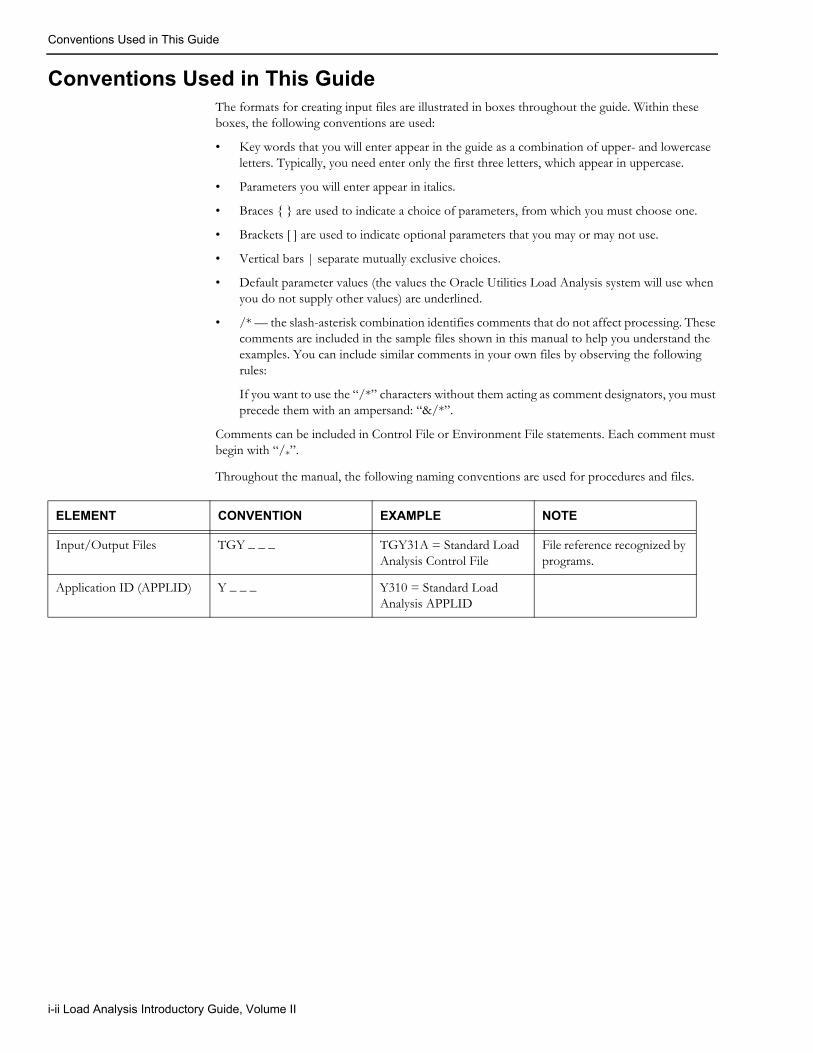
Conventions Used in This GuideThe formats for creating input files are illustrated in boxes throughout the guide. Within these boxes, the following conventions are used:
• Key words that you will enter appear in the guide as a combination of upper- and lowercase letters. Typically, you need enter only the first three letters, which appear in uppercase.
• Parameters you will enter appear in italics.
• Braces { } are used to indicate a choice of parameters, from which you must choose one.
• Brackets [ ] are used to indicate optional parameters that you may or may not use.
• Vertical bars | separate mutually exclusive choices.
• Default parameter values (the values the Oracle Utilities Load Analysis system will use when you do not supply other values) are underlined.
• /* — the slash-asterisk combination identifies comments that do not affect processing. These comments are included in the sample files shown in this manual to help you understand the examples. You can include similar comments in your own files by observing the following rules:
If you want to use the “/*” characters without them acting as comment designators, you must precede them with an ampersand: “&/*”.
Comments can be included in Control File or Environment File statements. Each comment must begin with “/*”.
Throughout the manual, the following naming conventions are used for procedures and files.
ELEMENT CONVENTION EXAMPLE NOTE
Input/Output Files TGY _ _ _ TGY31A = Standard Load Analysis Control File
File reference recognized by programs.
Application ID (APPLID) Y _ _ _ Y310 = Standard Load Analysis APPLID
i-ii Load Analysis Introductory Guide, Volume II
Other Load Analysis Documentation
Other Load Analysis DocumentationBelow are descriptions of other documentation that you may find helpful.
• The Oracle Utilities Load Analysis Quick Reference Guide — A concise summary of procedure names, input file commands and parameters, standard codes, and other essential information for the basic Oracle Utilities Load Analysis system and its extensions. It is a very useful tool to have at hand while you are working with Oracle Utilities Load Analysis.
• The Oracle Utilities Load Analysis Load Data Management User’s Guide — The companion to this manual, explains how to apply Oracle Utilities Load Analysis to build and maintain reliable databases of customer interval data for analysis, billing, and other important purposes.
• Oracle Utilities Load Analysis System Installation Guide/Oracle Utilities Load Analysis Configuration Guide — Explain how to install, customize, and maintain Oracle Utilities Load Analysis as a standalone system, or as a client/server system.
• Oracle Utilities Load Analysis User’s Guide — Explains how to use the graphical user interface of Oracle Utilities Load Analysis to “submit jobs” — that is, how to select a desired program, create and specify the necessary configurations, and view the results. This guide covers the mechanics of how to use Oracle Utilities Load Analysis. This guide should be used as a secondary companion piece to the Oracle Utilities Load Analysis Load Data Management User’s Guide and the Oracle Utilities Load Analysis Load Data Analysis User’s Guide.
In addition, there is a wide variety of optional programs, called “Bundles,” that add additional capabilities to the base Oracle Utilities Load Analysis package. One or more of these programs may be in use at your facility. With the exception of a few programs documented in the Introductory Guides, most of these Bundles are delivered with their own manuals.
How To Get HelpOccasionally, as you work with Oracle Utilities Load Analysis you may encounter an error message or other problem that you cannot decipher on your own. As a Oracle Utilities Load Analysis customer (current, on annual extended maintenance), you can contact Oracle Support personnel at http://metalink.oracle.com.
My Oracle Support offers you secure, real-time access to Oracle experts on the complete Oracle Utilities Load Analysis system. It also provides groundbreaking personalized & proactive support capabilities that help reduce unplanned down time and improve system stability. Leverage the Internet for immediate access to 24/7 support and get the critical and timely information you need for running your business.
Before contacting, please prepare the following information:
• Job directory containing the error
• Anything else that you think might aid in diagnosing the problem.
i-iii

Other Load Analysis Documentation
i-iv Load Analysis Introductory Guide, Volume II
Chapter 1Load Research and the Oracle Utilities Load
Analysis System
This chapter is a useful introduction for anyone unfamiliar with load research and the Oracle Utilities Load Analysis system. It describes the basic concepts of load research, and explains how accurate load research can benefit a utility and its customers.
The chapter then gives a brief overview of the entire Oracle Utilities Load Analysis System — including the Load Data Management Subsystem, the Load Analysis Subsystem, and the optional Bundles. Topics covered in this chapter are:
• What Is Load Research?
• How Do Utilities Conduct Load Research?
• What Does Oracle Utilities Load Analysis Do?
Load Research and the Oracle Utilities Load Analysis System 1-1
What Is Load Research?
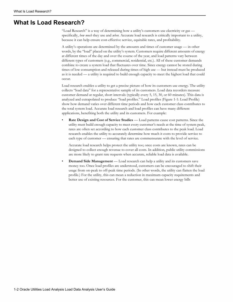
What Is Load Research?“Load Research” is a way of determining how a utility’s customers use electricity or gas — specifically, how much they use and when. Accurate load research is critically important to a utility, because it can help ensure cost-effective service, equitable rates, and profitability.
A utility’s operations are determined by the amounts and times of customer usage — in other words, by the “load” placed on the utility’s system. Customers require different amounts of energy at different times of the day and over the course of the year, and load patterns vary between different types of customers (e.g., commercial, residential, etc.). All of these customer demands combine to create a system load that fluctuates over time. Since energy cannot be stored during times of low consumption and released during times of high use — but instead must be produced as it is needed — a utility is required to build enough capacity to meet the highest load that could occur.
Load research enables a utility to get a precise picture of how its customers use energy. The utility collects “load data” for a representative sample of its customers. Load data recorders measure customer demand at regular, short intervals (typically every 5, 15, 30, or 60 minutes). This data is analyzed and extrapolated to produce “load profiles.” Load profiles (Figure 1-1: Load Profile) show how demand varies over different time periods and how each customer class contributes to the total system load. Accurate load research and load profiles can have many different applications, benefiting both the utility and its customers. For example:
• Rate Design and Cost of Service Studies — Load patterns cause cost patterns. Since the utility must build enough capacity to meet every customer’s needs at the time of system peak, rates are often set according to how each customer class contributes to the peak load. Load research enables the utility to accurately determine how much it costs to provide service to each type of customer — ensuring that rates are commensurate with the level of service.
Accurate load research helps protect the utility too; once costs are known, rates can be designed to collect enough revenue to cover all costs. In addition, public utility commissions are more likely to grant rate requests when accurate, reliable load data is available.
• Demand Side Management — Load research can help a utility and its customers save money too. Once load profiles are understood, customers can be encouraged to shift their usage from on-peak to off-peak time periods. (In other words, the utility can flatten the load profile.) For the utility, this can mean a reduction in maximum capacity requirements and better use of existing resources. For the customer, this can mean lower energy bills
1-2 Oracle Utilities Load Analysis Load Data Analysis User’s Guide
What Is Load Research?
.
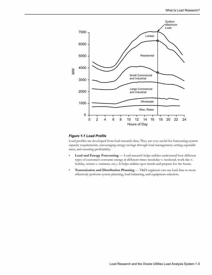
Figure 1-1 Load ProfileLoad profiles are developed from load research data. They are very useful for forecasting system capacity requirements, encouraging energy savings through load management, setting equitable rates, and ensuring profitability.
• Load and Energy Forecasting — Load research helps utilities understand how different types of customers consume energy at different times (weekday v. weekend, work day v. holiday, winter v. summer, etc.). It helps utilities spot trends and prepare for the future.
• Transmission and Distribution Planning — T&D engineers can use load data to more effectively perform system planning, load balancing, and equipment selection.
Losses
0 2 4 6 8 10 12 14 16 18 20 22 24
7000
6000
5000
4000
3000
2000
1000
0
Residential
Small Commercialand Industrial
Large Commercialand Industrial
Wholesale
Misc. Rates
Hours of Day
MW
SystemMaximumLoad
Load Research and the Oracle Utilities Load Analysis System 1-3
How Do Utilities Conduct Load Research?
How Do Utilities Conduct Load Research?Each utility has its own way of conducting load research, but some general steps can be outlined.
First, the utility identifies its major customer classes — for example, residential, commercial, industrial, and agricultural. Then, a small sample group is identified for each customer class. This is necessary because it is prohibitively expensive to obtain load data for each and every customer. Of course, for billing purposes all customers are metered to determine how much energy they consume during a given time period, such as kilowatt hours per month. While useful to supplement load research, this data is too limited to serve as the foundation for load research applications. Load research requires measurement of demand at regular, short intervals — that is, every 5, 10, 15, 30 or 60 minutes. Such measurement requires more effort and more sophisticated equipment — such as “digital pulse recorders” or “solid state devices.” Rather than installing expensive instruments at every customer site, a small but statistically-reliable sample of the total group is selected for monitoring. After the load data has been collected and validated for each sample group, it is analyzed and extrapolated to represent the entire population — providing an accurate picture of the amounts and time of energy consumption by each customer class (Figure 1-1: Load Profile).
For load research analysts, a key challenge is to design samples that will provide accurate pictures without costing a great deal. The number of expensive monitoring devices used to obtain the sample needs to be kept at a minimum, for example.
Traditionally, analysts have designed one sample for each customer class, aiming for accuracy at a particular time period — usually the peak hour of the year. PURPA standards require utilities to achieve at least 90% confidence with a 10% accuracy at the peak hour (the “90-10” rule).
Note: PURPA — the Public Utility Regulatory Policies Act — was signed into law on November 8, 1978. It established a set of procedures and requirements for state utility commissions and electric and gas utilities and was designed to standardize rate making and encourage conservation.
In today’s demanding environment, however, other departments within the company, as well as important customers, are pressing analysts to go well beyond these standards. They need samples that are more accurate and more creative — for example, samples that are accurate for more than one period, such as winter and summer peak hours, and samples that incorporate special characteristics, such as single family homes vs. apartments. Thanks to increasingly sophisticated computer tools such as Oracle Utilities Load Analysis, analysts can respond to such demands.
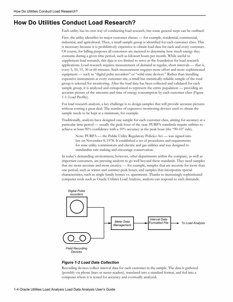
Figure 1-2 Load Data CollectionRecording devices collect interval data for each customer in the sample. The data is gathered (possibly via phone lines or meter readers), translated into a standard format, and fed into a computer where it is tested for accuracy and eventually analyzed.
Meter Data Management
Interval DataFormatted File To Load Analysis
Digital Pulserecorders
Field RecordingDevices
1-4 Oracle Utilities Load Analysis Load Data Analysis User’s Guide
How Do Utilities Conduct Load Research?
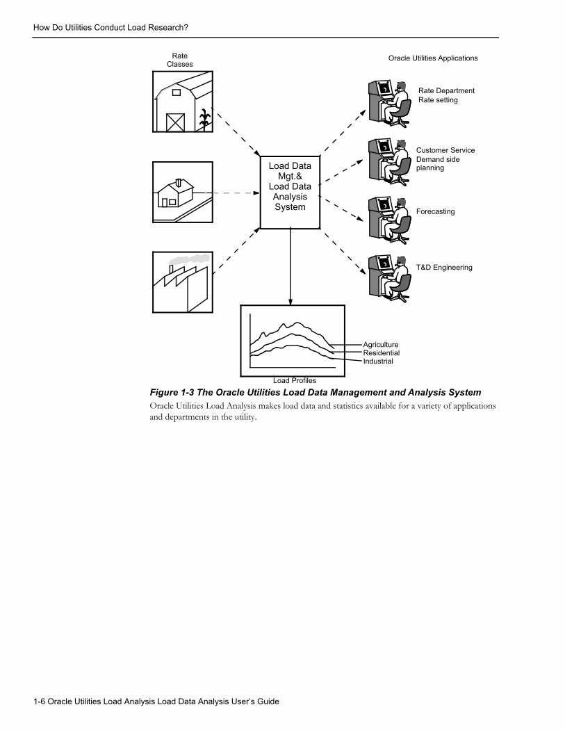
What Does Oracle Utilities Load Analysis Do?Oracle Utilities Load Analysis is a software program for the management and analysis of load research data. Originally developed to help clients meet PURPA requirements, Oracle Utilities Load Analysis has been enhanced and expanded over time to become a broad-based system for a variety of load research applications (Figure 1-3: The Oracle Utilities Load Data Management and Analysis System). Oracle Utilities Load Analysis is now in use at more than seventy utilities across the world, and is the most widely-used system of its kind.
The basic Oracle Utilities Load Analysis package consists of two subsystems: Load Data Management and Load Data Analysis (Figure 1-4: Overview of the Oracle Utilities Load Data Management and Analysis System).
The functions of the Load Data Management Subsystem are: to accept load data from a variety of sources; to ensure that the data is complete, consistent, and accurate; and to make it available for reporting and analysis (Figure 1-4: Overview of the Oracle Utilities Load Data Management and Analysis System). The Load Analysis Subsystem applies complex formulas to the load data in order to generate meaningful statistics on customer, class, and system load patterns, and it produces both standard and ad hoc reports. Both subsystems include programs for various “housekeeping” tasks such as data storage.
Additional programs are included with Oracle Utilities Load Analysis system — adding further data management and analysis functions, such as advanced sample design, additional data validation, and reporting. Here is a brief description of each:
Individual Customer Analysis (ICA) — produces time-of-use, entire period and average day statistics and reports. Different time-of-use schedules can be applied to the same customer in a single run enabling what-if analysis. ICA produces statistics for interruption and load control periods, and can compute statistics for non-contiguous time periods in the same analysis.
Load Research and the Oracle Utilities Load Analysis System 1-5
How Do Utilities Conduct Load Research?
Figure 1-3 The Oracle Utilities Load Data Management and Analysis System Oracle Utilities Load Analysis makes load data and statistics available for a variety of applications and departments in the utility.
Load Data Mgt.&
Load DataAnalysisSystem
RateClasses
Oracle Utilities Applications
AgricultureResidentialIndustrial
Load Profiles
Rate DepartmentRate setting
Customer ServiceDemand sideplanning
Forecasting
T&D Engineering
1-6 Oracle Utilities Load Analysis Load Data Analysis User’s Guide
How Do Utilities Conduct Load Research?
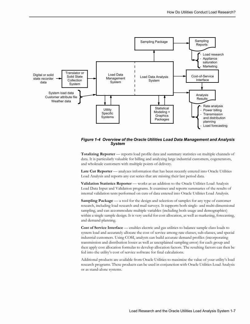
Figure 1-4 Overview of the Oracle Utilities Load Data Management and Analysis System
Totalizing Reporter — reports load profile data and summary statistics on multiple channels of data. It is particularly valuable for billing and analyzing large industrial customers, cogenerators, and wholesale customers with multiple points of delivery.
Late Cut Reporter — analyzes information that has been recently entered into Oracle Utilities Load Analysis and reports any cut series that are missing their last period data.
Validation Statistics Reporter — works as an addition to the Oracle Utilities Load Analysis Load Data Input and Validation programs. It examines and reports summaries of the results of internal validation tests performed on cuts of data entered into Oracle Utilities Load Analysis.
Sampling Package — a tool for the design and selection of samples for any type of customer research, including load research and mail surveys. It supports both single- and multi-dimensional sampling, and can accommodate multiple variables (including both usage and demographics) within a single sample design. It is very useful for cost allocation, as well as marketing, forecasting, and demand planning.
Cost of Service Interface — enables electric and gas utilities to balance sample class loads to system load and accurately allocate the cost of service among rate classes, sub-classes, and special industrial customers. Using COSI, analysts can build accurate demand profiles (incorporating transmission and distribution losses as well as unexplained sampling error) for each group and then apply cost allocation formulas to develop allocation factors. The resulting factors can then be fed into the utility’s cost of service software for final calculations.
Additional products are available from Oracle Utilities to maximize the value of your utility’s load research programs. These products can be used in conjunction with Oracle Utilities Load Analysis or as stand-alone systems.
Sampling Package SamplingReports
Cost-of-ServiceInterface
AnalysisResults
StatisticalModeling +GraphicsPackages
UtilitySpecificSystems
Translator orSolid StateCollectionSystem
Load DataManagement
SystemLoad Data Analysis
System
- Rate analysis- Power billing- Transmission
and distributionplanning
- Load forecasting
System load dataCustomer attribute file
Weather data
Digital or solid state recorder
data
- Load research- Appliance
saturation- Marketing
Load Research and the Oracle Utilities Load Analysis System 1-7

How Do Utilities Conduct Load Research?
1-8 Oracle Utilities Load Analysis Load Data Analysis User’s Guide
Chapter 2Overview of the Oracle Utilities Load Data
Analysis System
This chapter introduces the Oracle Utilities Load Data Analysis Subsystem programs and tablesets, and describes the steps you will follow when working with the subsystem. If you are a new Oracle Utilities Load Analysis user, you should read this chapter.
• What Is the Purpose of the Load Data Analysis System?
• How Does It Work?
• How Is the LAS Structured?
• Working With the Load Data Analysis Subsystem — What Steps Do You Follow?
Overview of the Oracle Utilities Load Data Analysis System 2-1
What Is the Purpose of the Load Data Analysis System?
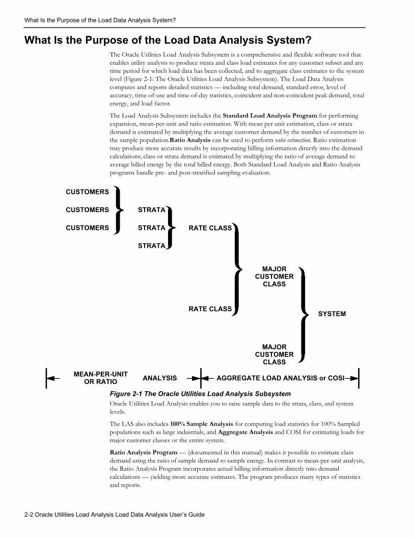
What Is the Purpose of the Load Data Analysis System?The Oracle Utilities Load Analysis Subsystem is a comprehensive and flexible software tool that enables utility analysts to produce strata and class load estimates for any customer subset and any time period for which load data has been collected, and to aggregate class estimates to the system level (Figure 2-1: The Oracle Utilities Load Analysis Subsystem). The Load Data Analysis computes and reports detailed statistics — including total demand, standard error, level of accuracy, time-of-use and time-of-day statistics, coincident and non-coincident peak demand, total energy, and load factor.
The Load Analysis Subsystem includes the Standard Load Analysis Program for performing expansion, mean-per-unit and ratio estimation. With mean per unit estimation, class or strata demand is estimated by multiplying the average customer demand by the number of customers in the sample population.Ratio Analysis can be used to perform ratio estimation. Ratio estimation may produce more accurate results by incorporating billing information directly into the demand calculations; class or strata demand is estimated by multiplying the ratio of average demand to average billed energy by the total billed energy. Both Standard Load Analysis and Ratio Analysis programs handle pre- and post-stratified sampling evaluation.
Figure 2-1 The Oracle Utilities Load Analysis SubsystemOracle Utilities Load Analysis enables you to raise sample data to the strata, class, and system levels.
The LAS also includes 100% Sample Analysis for computing load statistics for 100% Sampled populations such as large industrials, and Aggregate Analysis and COSI for estimating loads for major customer classes or the entire system.
Ratio Analysis Program — (documented in this manual) makes it possible to estimate class demand using the ratio of sample demand to sample energy. In contrast to mean-per-unit analysis, the Ratio Analysis Program incorporates actual billing information directly into demand calculations — yielding more accurate estimates. The program produces many types of statistics and reports.
CUSTOMERS
CUSTOMERS
CUSTOMERS
STRATA
STRATA
STRATA
RATE CLASS
RATE CLASS
MAJORCUSTOMER
CLASS
MAJORCUSTOMER
CLASS
SYSTEM
MEAN-PER-UNITOR RATIO ANALYSIS AGGREGATE LOAD ANALYSIS or COSI
2-2 Oracle Utilities Load Analysis Load Data Analysis User’s Guide
What Is the Purpose of the Load Data Analysis System?
In addition, the Load Data Analysis Subsystem offers three more optional extensions that provide further analysis capabilities:
Domains Analysis — (documented in Chapter 11: Estimating Loads for Subpopulations Using the Domains Analysis Programs (Y350 or Y360)) enables analysts to produce estimates of total loads for sub-populations in an existing customer sample (for example, customers with air conditioning or grocery stores that are open twenty-four hours a day). This type of analysis is extremely useful for rate design, load management, forecasting, and marketing studies.
Coincident Peak Analysis Program — (documented in this manual) makes it possible to produce estimates of rate class coincident peak demand and its corresponding error for up to twelve periods. It helps determine the responsibility of a rate class towards cost, providing a more accurate measure than approaches based on a single hour of demand. Coincident Peak Analysis uses both mean-per-unit and ratio estimation techniques.
Oracle Utilities Load Analysis also makes individual customer statistics and group statistics available for ad hoc analysis, either by the Oracle Utilities Load Analysis Transformation Program or by external programs such as spreadsheet packages and statistical analysis packages.
Altogether, the Load Data Analysis Subsystem is both powerful and flexible, giving you many options in terms of data selection, analysis methodologies and parameters, and reporting capabilities. These features simplify and streamline sensitivity analysis, and enable you to quickly and efficiently respond to requests for different types of analyses.
How Does It Work?The Load Data Analysis Subsystem accepts interval load data from the Load Data Management Subsystem or other sources. (“Interval load data” refers to a series of values representing each individual customer’s demand, measured at regular, short time intervals.) You can select data for analysis by specifying the date range, customer subset, and criteria for acceptable data quality.
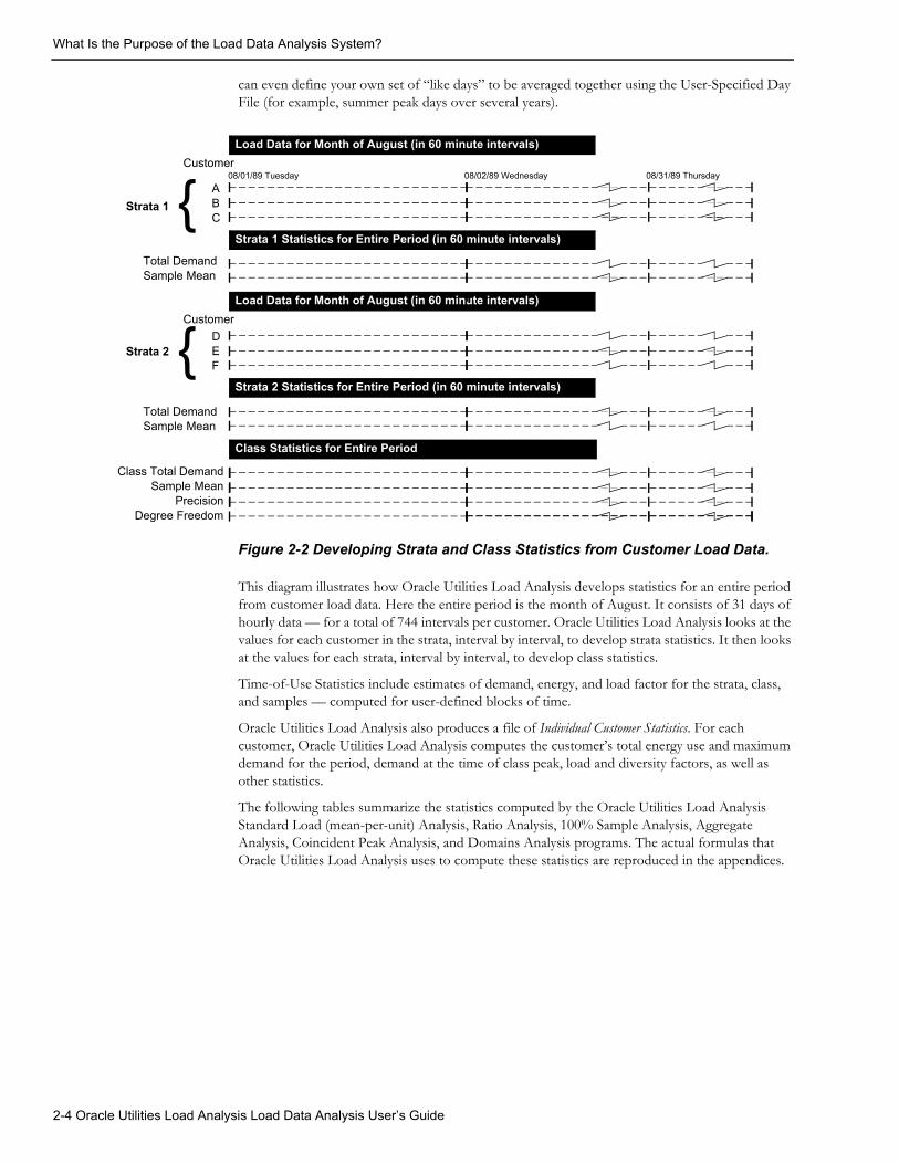
According to parameters you supply, Oracle Utilities Load Analysis first develops strata and class statistics by combining and analyzing customer load data (Figure 2-2: Developing Strata and Class Statistics from Customer Load Data.), interval by interval over the entire analysis period. The resulting statistics are called Entire Period Demands.
At the strata level, these statistics are estimates of total demand and the standard error — for each interval in the analysis period. Oracle Utilities Load Analysis combines the strata estimates to obtain class-level estimates of total demand, standard error, precision, and degrees of freedom — also interval by interval over the entire period.
In addition to statistics for the entire period, Oracle Utilities Load Analysis looks at the interval load data in different ways to calculate two other types of statistics called Average Day and Time-of-Use Statistics.
Average Day Statistics are computed from customer load data across a set of like days. For example, to estimate how a class uses electricity on Saturdays (e.g., “average Saturday”), Oracle Utilities Load Analysis looks at each interval of every Saturday for each customer in the class. You
Overview of the Oracle Utilities Load Data Analysis System 2-3
What Is the Purpose of the Load Data Analysis System?
can even define your own set of “like days” to be averaged together using the User-Specified Day File (for example, summer peak days over several years).
Figure 2-2 Developing Strata and Class Statistics from Customer Load Data.
This diagram illustrates how Oracle Utilities Load Analysis develops statistics for an entire period from customer load data. Here the entire period is the month of August. It consists of 31 days of hourly data — for a total of 744 intervals per customer. Oracle Utilities Load Analysis looks at the values for each customer in the strata, interval by interval, to develop strata statistics. It then looks at the values for each strata, interval by interval, to develop class statistics.
Time-of-Use Statistics include estimates of demand, energy, and load factor for the strata, class, and samples — computed for user-defined blocks of time.
Oracle Utilities Load Analysis also produces a file of Individual Customer Statistics. For each customer, Oracle Utilities Load Analysis computes the customer’s total energy use and maximum demand for the period, demand at the time of class peak, load and diversity factors, as well as other statistics.
The following tables summarize the statistics computed by the Oracle Utilities Load Analysis Standard Load (mean-per-unit) Analysis, Ratio Analysis, 100% Sample Analysis, Aggregate Analysis, Coincident Peak Analysis, and Domains Analysis programs. The actual formulas that Oracle Utilities Load Analysis uses to compute these statistics are reproduced in the appendices.
Strata 1ABC
Customer 08/01/89 Tuesday 08/02/89 Wednesday 08/31/89 Thursday
Load Data for Month of August (in 60 minute intervals)
Total DemandSample Mean
Strata 1 Statistics for Entire Period (in 60 minute intervals)
Strata 2DEF
CustomerLoad Data for Month of August (in 60 minute intervals)
Total DemandSample Mean
Strata 2 Statistics for Entire Period (in 60 minute intervals)
Class Statistics for Entire Period
Strata 1 Statistics for Entire Period (in 60 minute intervals)
Class Total DemandSample Mean
PrecisionDegree Freedom
{
{
2-4 Oracle Utilities Load Analysis Load Data Analysis User’s Guide
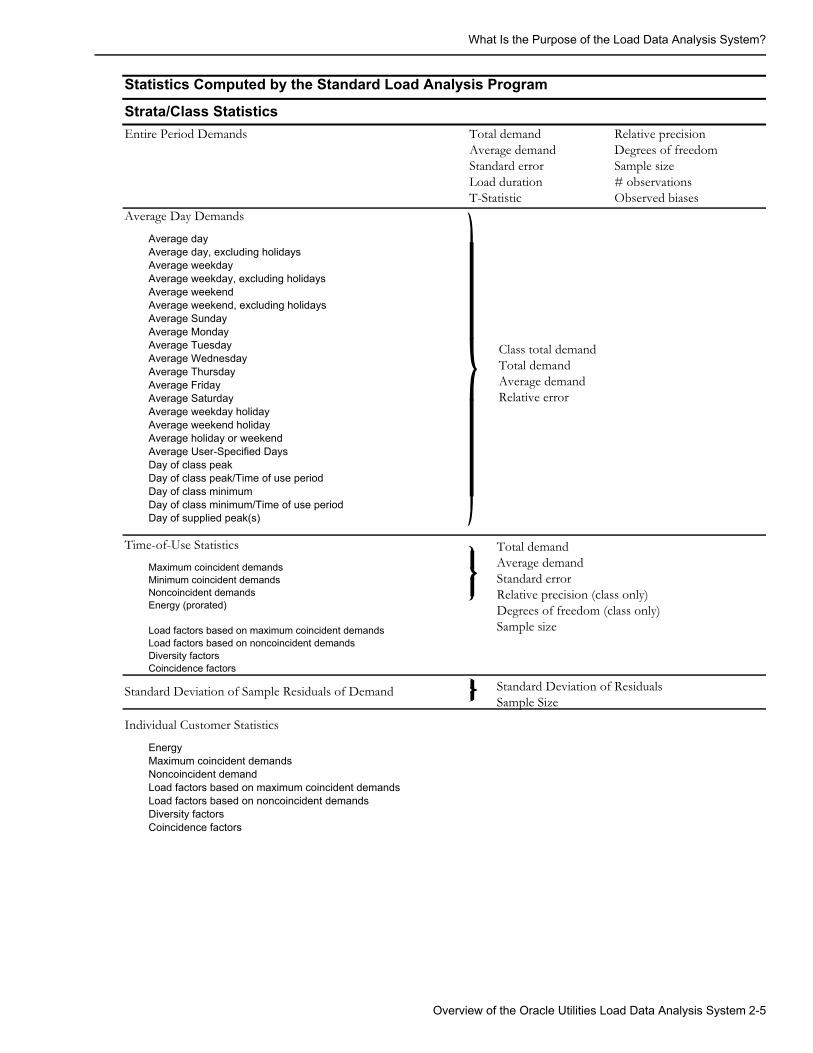
What Is the Purpose of the Load Data Analysis System?
Individual Customer Statistics
EnergyMaximum coincident demandsNoncoincident demandLoad factors based on maximum coincident demandsLoad factors based on noncoincident demandsDiversity factorsCoincidence factors
Statistics Computed by the Standard Load Analysis Program
Strata/Class StatisticsEntire Period Demands Total demand
Average demandStandard errorLoad durationT-Statistic
Relative precisionDegrees of freedomSample size# observationsObserved biases
Average Day Demands
Average dayAverage day, excluding holidaysAverage weekdayAverage weekday, excluding holidaysAverage weekendAverage weekend, excluding holidaysAverage SundayAverage MondayAverage TuesdayAverage WednesdayAverage ThursdayAverage FridayAverage SaturdayAverage weekday holidayAverage weekend holidayAverage holiday or weekendAverage User-Specified DaysDay of class peakDay of class peak/Time of use periodDay of class minimumDay of class minimum/Time of use periodDay of supplied peak(s)
Class total demandTotal demandAverage demandRelative error
Time-of-Use Statistics
Maximum coincident demandsMinimum coincident demandsNoncoincident demandsEnergy (prorated)
Load factors based on maximum coincident demandsLoad factors based on noncoincident demandsDiversity factorsCoincidence factors
Total demandAverage demandStandard errorRelative precision (class only)Degrees of freedom (class only)Sample size
Standard Deviation of Sample Residuals of Demand Standard Deviation of ResidualsSample Size
Overview of the Oracle Utilities Load Data Analysis System 2-5
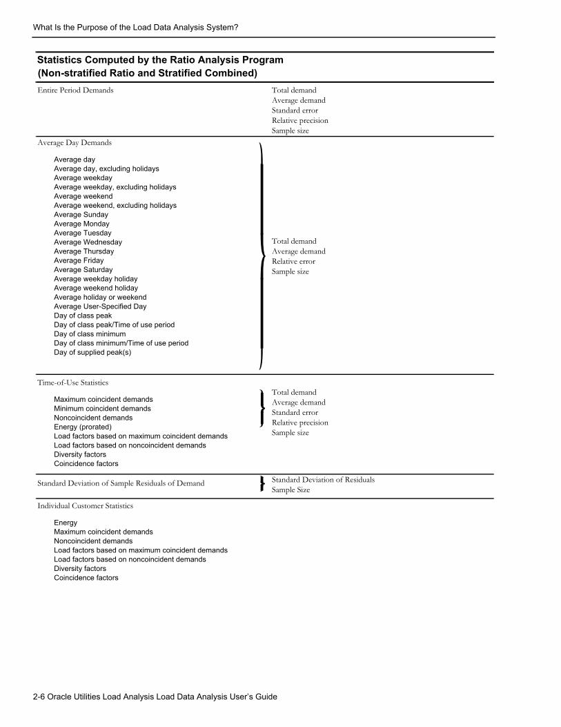
What Is the Purpose of the Load Data Analysis System?
Statistics Computed by the Ratio Analysis Program(Non-stratified Ratio and Stratified Combined)Entire Period Demands Total demand
Average demandStandard errorRelative precisionSample size
Average Day Demands
Average dayAverage day, excluding holidaysAverage weekdayAverage weekday, excluding holidaysAverage weekendAverage weekend, excluding holidaysAverage SundayAverage MondayAverage TuesdayAverage WednesdayAverage ThursdayAverage FridayAverage SaturdayAverage weekday holidayAverage weekend holidayAverage holiday or weekendAverage User-Specified DayDay of class peakDay of class peak/Time of use periodDay of class minimumDay of class minimum/Time of use periodDay of supplied peak(s)
Total demandAverage demandRelative errorSample size
Time-of-Use Statistics
Maximum coincident demandsMinimum coincident demandsNoncoincident demandsEnergy (prorated)Load factors based on maximum coincident demandsLoad factors based on noncoincident demandsDiversity factorsCoincidence factors
Total demandAverage demandStandard errorRelative precisionSample size
Individual Customer Statistics
EnergyMaximum coincident demandsNoncoincident demandsLoad factors based on maximum coincident demandsLoad factors based on noncoincident demandsDiversity factorsCoincidence factors
Standard Deviation of Sample Residuals of Demand Standard Deviation of ResidualsSample Size
2-6 Oracle Utilities Load Analysis Load Data Analysis User’s Guide
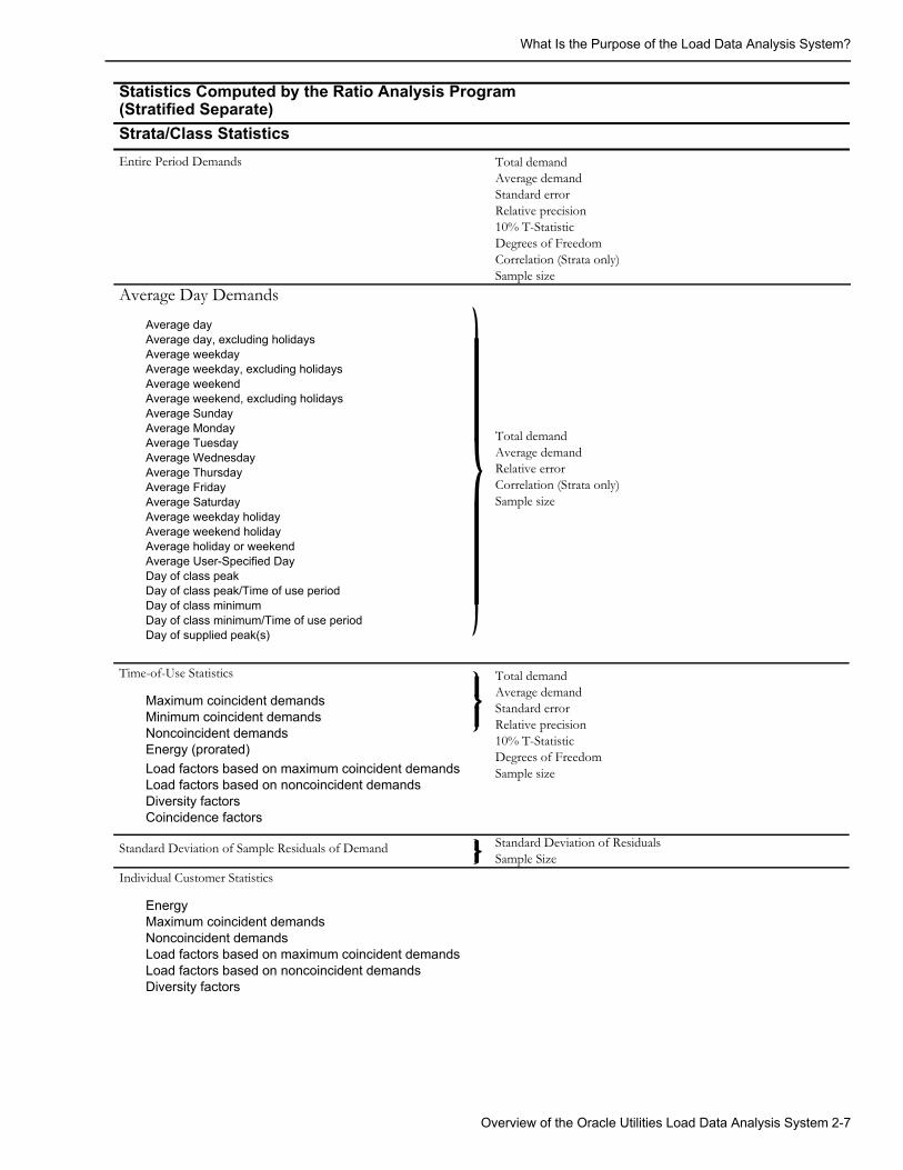
What Is the Purpose of the Load Data Analysis System?
Statistics Computed by the Ratio Analysis Program(Stratified Separate)
Entire Period Demands Total demandAverage demandStandard errorRelative precision10% T-StatisticDegrees of FreedomCorrelation (Strata only)Sample size
Average Day Demands
Average dayAverage day, excluding holidaysAverage weekdayAverage weekday, excluding holidaysAverage weekendAverage weekend, excluding holidaysAverage SundayAverage MondayAverage TuesdayAverage WednesdayAverage ThursdayAverage FridayAverage SaturdayAverage weekday holidayAverage weekend holidayAverage holiday or weekendAverage User-Specified DayDay of class peakDay of class peak/Time of use periodDay of class minimumDay of class minimum/Time of use periodDay of supplied peak(s)
Total demandAverage demandRelative errorCorrelation (Strata only)Sample size
Time-of-Use Statistics
Maximum coincident demandsMinimum coincident demandsNoncoincident demandsEnergy (prorated)Load factors based on maximum coincident demandsLoad factors based on noncoincident demandsDiversity factorsCoincidence factors
Total demandAverage demandStandard errorRelative precision10% T-StatisticDegrees of FreedomSample size
Individual Customer Statistics
EnergyMaximum coincident demandsNoncoincident demandsLoad factors based on maximum coincident demandsLoad factors based on noncoincident demandsDiversity factors
Strata/Class Statistics
Standard Deviation of Sample Residuals of Demand Standard Deviation of ResidualsSample Size
Overview of the Oracle Utilities Load Data Analysis System 2-7
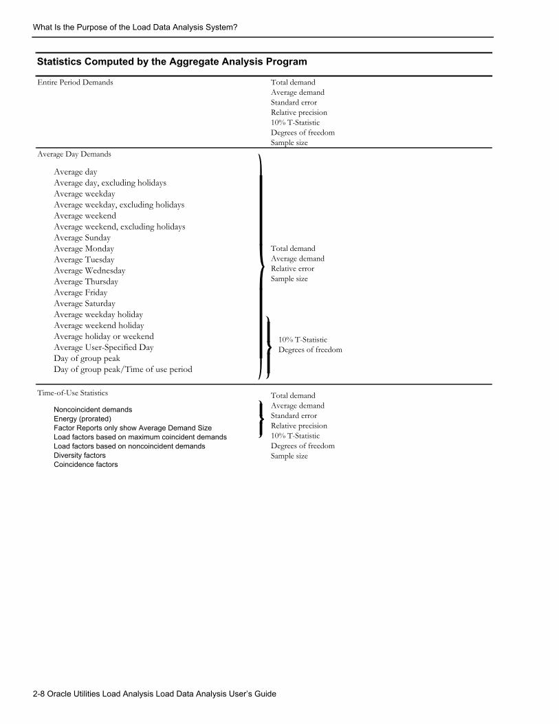
What Is the Purpose of the Load Data Analysis System?
Statistics Computed by the Aggregate Analysis Program
Entire Period Demands Total demandAverage demandStandard errorRelative precision10% T-StatisticDegrees of freedomSample size
Average Day Demands
Average dayAverage day, excluding holidaysAverage weekdayAverage weekday, excluding holidaysAverage weekendAverage weekend, excluding holidaysAverage SundayAverage MondayAverage TuesdayAverage WednesdayAverage ThursdayAverage FridayAverage SaturdayAverage weekday holidayAverage weekend holidayAverage holiday or weekendAverage User-Specified DayDay of group peakDay of group peak/Time of use period
Total demandAverage demandRelative errorSample size
Time-of-Use Statistics
Noncoincident demandsEnergy (prorated)Factor Reports only show Average Demand SizeLoad factors based on maximum coincident demandsLoad factors based on noncoincident demandsDiversity factorsCoincidence factors
Total demandAverage demandStandard errorRelative precision10% T-StatisticDegrees of freedomSample size
10% T-StatisticDegrees of freedom
2-8 Oracle Utilities Load Analysis Load Data Analysis User’s Guide
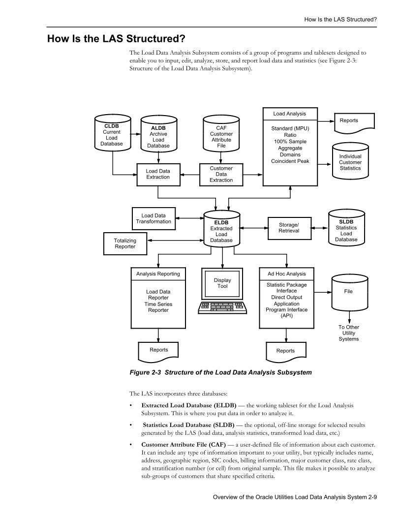
How Is the LAS Structured?
How Is the LAS Structured?The Load Data Analysis Subsystem consists of a group of programs and tablesets designed to enable you to input, edit, analyze, store, and report load data and statistics (see Figure 2-3: Structure of the Load Data Analysis Subsystem).
Figure 2-3 Structure of the Load Data Analysis Subsystem
The LAS incorporates three databases:
• Extracted Load Database (ELDB) — the working tableset for the Load Analysis Subsystem. This is where you put data in order to analyze it.
• Statistics Load Database (SLDB) — the optional, off-line storage for selected results generated by the LAS (load data, analysis statistics, transformed load data, etc.)
• Customer Attribute File (CAF) — a user-defined file of information about each customer. It can include any type of information important to your utility, but typically includes name, address, geographic region, SIC codes, billing information, major customer class, rate class, and stratification number (or cell) from original sample. This file makes it possible to analyze sub-groups of customers that share specified criteria.
ALDBArchive
LoadDatabase
Load DataExtraction
CustomerData
Extraction
Load AnalysisReports
Load DataTransformation ELDB
ExtractedLoad
Database
Storage/Retrieval
SLDBStatistics
LoadDatabase
DisplayTool
To OtherUtility
Systems
Reports Reports
Standard (MPU)Ratio
100% SampleAggregateDomains
Coincident PeakIndividualCustomerStatistics
Ad Hoc Analysis
Statistic PackageInterface
Direct OutputApplication
Program Interface(API)
Analysis Reporting
Load DataReporter
Time SeriesReporter
CAFCustomerAttribute
File
CLDBCurrent
LoadDatabase
File
TotalizingReporter
Overview of the Oracle Utilities Load Data Analysis System 2-9
How Is the LAS Structured?
The LAS extracts data for analysis from two tablesets in the Load Data Management Subsystem:
• Archive Load Database (ALDB) — the optional, off-line storage for data that has been validated with the Load Data Management Subsystem. The ALDB is typically the source of data for analysis.
• Current Load Database (CLDB) — the working tableset for the Load Data Management Subsystem. Data in the CLDB has been converted to the standard Oracle Utilities Load Analysis load data format, but may or may not have been validated for analysis. The CLDB is an alternate source of data for analysis.
The LAS also includes several programs. Their uses are described on the following page.
Working With the Load Data Analysis Subsystem — What Steps Do You Follow?
The Load Data Analysis Subsystem is very flexible, allowing you to tailor its applications to the particular needs of your utility. As an introduction, the basic sequence of steps for using it are outlined below. Following chapters will examine each operation — along with its many options — in detail.
Step 1: Inputting DataThe first step is to bring selected data into the Extracted Load Database (ELDB), where you can apply the Oracle Utilities Load Analysis analysis programs to it. You can use the Load Data Extraction Program (Y240) to extract it from the Archive Load Database (ALDB) or the Current Load Database (CLDB), or you can enter it manually using the Manual Entry Program (Y220). Obviously, the quality of an analysis is dependent upon the quality of the sample data, so you will want to be sure that the data you enter is as complete and accurate as possible.
If you wish to analyze only data for customers who fit a particular profile, you can use the Customer Data Extraction Function (Y110) — a.k.a. the Key Generator — to extract customer data according to the specific criteria you want.
Step 2: Modifying DataUnder certain circumstances, you may wish to modify data in the ELDB before analysis. For example, if you were to run analyses for planning purposes, you would probably replace outages with estimated values.
Note: Although outages reflect actual customer usage, they are likely to be the results of abnormal events of a particular past period and are not appropriate to include in forecasts of use. In such a case, you would first review the data in the ELDB using the Load Data Reporter (ELDB) Program (Y420), or Interval Data Manager (IDM). Once you have identified the data you wish to modify, you would use the Load Data Editor (ELDB) Program (Y630) or IDM.
2-10 Oracle Utilities Load Analysis Load Data Analysis User’s Guide
How Is the LAS Structured?
Step 3: Analysis — Expanding Data to Class Level EstimatesOnce the interval data is in the ELDB, you can apply either the Standard Load Analysis Program (Y310) (for Mean Per Unit analysis) or the Ratio Analysis Program (Y330) to it. These programs calculate statistics for single analysis groups such as a strata or rate class. The 100% Sample Analysis Program (Y380) is also available to calculate statistics for 100% sampled populations, such as large industrials.
Whether you use Standard Load Analysis or Ratio Analysis, your choice of program will depend upon your objectives, whether or not billed energy data is available, and possibly your sample design and quality. This data may come from books and records, or you may use the Billed Energy Program (Y230) to derive the values from interval demand data in a Oracle Utilities Load Analysis database.
Both the Standard Load and Ratio Analysis programs perform stratified or non-stratified analysis and provide both pre- and post-stratification capability. The Ratio Analysis program offers two estimation techniques for stratified samples — Combined Estimate and Separate Estimate.
In addition, both Standard Load Analysis and Ratio Analysis compute and report an extensive variety of load statistics, including estimates of load profiles, energy, and relative precision. The programs write all calculated statistics as cuts to the ELDB for additional analysis and reporting. They also create a file of individual customer statistics that can be accessed by user programs.
Note: If you wish to analyze only customers who fit a particular profile, you can use the Key Generator (Y810 or X810) to select a subset of data in the ELDB for analysis.
Step 4: Analysis — Aggregating Class Estimates to the System LevelThe Aggregate Load Analysis Program (Y320) or the COSI subsystem enable you to combine the results of your analyses for individual analysis groups to obtain statistics for a major customer class or the entire system. The program can process statistical cuts from multiple sources (e.g., Standard Load Analysis, Separate Ratio Analysis, Combined Ratio Analysis, and 100% Sample Analysis) in a single run. Again, you can report any or all of the resulting statistics, and save them in the ELDB for additional analysis and reporting.
Step 5: ReportingOnce you have created a body of statistics using the Oracle UtilitiesOracle Utilities Load Analysis Analysis programs, you may want to produce special reports that highlight some subset of the results or provide additional information. Many different reporting programs are available. For example, the Time Series Reporter (Y410) is a useful tool for formatting reports of user-selected statistics in a neat, tabular format. The ELDB Summary Reporter gives a quick overview of the entire contents of the tableset, listing each record in the tableset along with its start time and percentage of acceptable data. The Load Data Reporter (ELDB) Program (Y420) enables you to take a comprehensive, detailed look at each statistic or load data record. The Interval Data Manager (IDM) enables you to quickly display load data and statistics in easy-to-understand graphs.
Step 6: Additional AnalysisIn addition to the standard analysis programs described above, Oracle Utilities Load Analysis supports ad hoc analysis.
Oracle Utilities Load Analysis also offers a Load Data Transformation (Y620) capability. Data Transformation enables you to create new data from existing data in the Extracted Load Database (ELDB) or Current Load Database (CLDB). For example, you can compute a customer’s power factor from KVA and KW. Load data transformations include standard arithmetic operations and functional operations.
Overview of the Oracle Utilities Load Data Analysis System 2-11
How Is the LAS Structured?
Optional extensions are available to further enhance the analysis capabilities of your Oracle Utilities Load Analysis system. Some or all of these extensions may be in use at your facility. They include: Domains Analysis (Y350, Y360) for computing statistically-reliable estimates for subgroups in preexisting samples; Coincident Peak Analysis (Y340) for calculating the estimate of the mean and corresponding sampling error for up to twelve periods of coincident peak demands and Totalizing Reporter (Y450) for reporting load profile data and summary statistics on multiple channels of data. Coincident Peak Analysis is documented in this manual. The others are documented in separate manuals. Contact your supervisor or Oracle Corporation for more information.
Step 7: Archiving Statistics and Load DataOracle Utilities Load Analysis gives you the option of archiving your statistics and load data to archive designated tablesets. Use the Archive/Delete Program (Y910) to move specified records from the Extracted Load Database to the Statistics Load Database (SLDB). The SLDB Key Generator Program (Y820) facilitates the process by enabling you to quickly specify records for archiving according to desired criteria.
Prior to moving data from the ELDB to the SLDB, you may want to examine the contents of the ELDB. The ELDB Summary Reporter (Y440) enables you to produce a hard copy list of the entire contents of the ELDB as well as useful statistics on the tableset (number of cuts, number of statistics, etc.).
Once records have been archived to the SLDB, you may find that you need to move them back to the ELDB for further analysis or examination. The SLDB Retrieval Program (Y960) makes this possible. The SLDB can be directly accessed from most Oracle Utilities Load Analysis programs.
You may also simply create new generations of ELDBs & CLDBs to store new data and manage what data is in each using the Q91x series of programs Move/Copy/Delete cuts.
2-12 Oracle Utilities Load Analysis Load Data Analysis User’s Guide
Chapter 3The Oracle Utilities Load Analysis Data Formats
In previous chapters we have often used the term “load data” to refer to the raw data that Oracle Utilities Load Analysis analyzes in order to generate statistics. In this chapter we will take a closer look at the kinds of information Oracle Utilities Load Analysis handles and how it is organized in the analysis subsystem. We will examine the formats for both load data and statistics.
This is a key chapter, and new Oracle Utilities Load Analysis users should be sure to read it. It defines many of the terms you will need to understand as you work with the Load Analysis Subsystem, including:
• ELDB Load Data Records
• Statistics Records
The Oracle Utilities Load Analysis Data Formats 3-1
The Oracle Utilities Load Analysis Subsystem stores and manipulates two major types of data (or cuts):
• Load Data — also called “time-series data” — finite sequences of discrete measurements of various quantities such as electric loads, voltage, temperature, and other variables that fluctuate over time. The terms “load data” and “interval data” are used throughout this discussion in a generic sense to cover all time-series data.
• Statistics — estimates of demand for various groups (customers, strata, samples, classes, and system) computed by the Load Analysis Subsystem.
This chapter examines the content and organization of both types of records in detail.
The Load Analysis Subsystem also uses a user-created Customer Attribute File to describe the characteristics of sampled customers. That file is described in Chapter 14: Key Generators — Shortcuts for Creating Input Files and Reports.
ELDB Load Data Records
Cuts, Cut Series, and Cut KeysOracle Utilities Load Analysis works with load data in units called “cuts” and “cut series” (Figure 3-1: Cuts and Cut Series).
• Cut — A cut is a record of load data for a single customer and channel number, covering a single, user-defined time period. Each cut has a unique start-time and stop-time. (Cuts are so named because they represent a slice of time in the ongoing measurement of a customer’s demand.)
3-2 Oracle Utilities Load Analysis Load Data Analysis User’s Guide
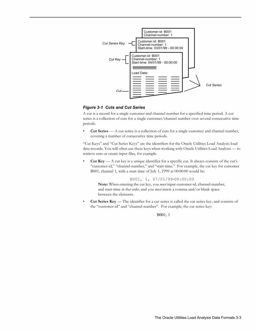
Figure 3-1 Cuts and Cut SeriesA cut is a record for a single customer and channel number for a specified time period. A cut series is a collection of cuts for a single customer/channel number over several consecutive time periods.
• Cut Series — A cut series is a collection of cuts for a single customer and channel number, covering a number of consecutive time periods.
“Cut Keys” and “Cut Series Keys” are the identifiers for the Oracle Utilities Load Analysis load data records. You will often use these keys when working with Oracle Utilities Load Analysis — to retrieve cuts or create input files, for example.
• Cut Key — A cut key is a unique identifier for a specific cut. It always consists of the cut’s “customer-id,” “channel-number,” and “start-time.” For example, the cut key for customer B001, channel 1, with a start-time of July 1, 1999 at 00:00:00 would be:
B001, 1, 07/01/99-00:00:00Note: When entering the cut key, you must input customer-id, channel-number, and start-time in that order, and you must insert a comma and/or blank space between the elements.
• Cut Series Key — The identifier for a cut series is called the cut series key, and consists of the “customer-id” and “channel-number”. For example, the cut series key:
B001, 1
Customer-id: B001Channel-number: 1
Customer-id: B001Channel-number: 1Start-time: 03/01/99 - 00:00:00
Customer-id: B001Channel-number: 1Start-time: 04/01/99 - 00:00:00
Load Data:
Cut Series
Cut
Cut Key
Cut Series Key
The Oracle Utilities Load Analysis Data Formats 3-3
would identify all cuts in a tableset with the customer-id “B001” and channel 1, regardless of their start-times.
Header and Interval Data in Load Data RecordsA Oracle Utilities Load Analysis cut consists of two parts:
• Header — a series of fixed-length fields that contain the cut key and other descriptive information about the cut.
• Interval Data — a series of values that represent the actual customer demand, measured at specified intervals. This data is stored as “energy,” but can be reported as “energy” or “demand.” The interval data portion of the cut can be any length when using Oracle Utilities Load Analysis.
Oracle Utilities Load Analysis also stores status codes in this portion of the record. Status codes indicate the quality of the load data, interval by interval.
Each field in the record is described in detail below and on the following pages. The fields are described in the order in which they appear on the report, and are pertinent to the Oracle Utilities Standard Format (.INP), although Oracle Utilities Load Analysis supports the .LSE format as well as the DataConnect format (.DAT).
• Customer-id is a unique 1- to 64-character identifier assigned to each customer, premise, data stream, or recording device by rate analysts or others at your utility.
Typically, the ID is assigned to the recording device when it is installed, and Oracle Utilities Load Analysis automatically preserves the ID with the cut. However, Oracle Utilities Load Analysis gives you the option of modifying the ID when the data is input to the CLDB or ELDB.
• Channel-number is an integer (0 to 32767) used to identify the port, register, or channel of the device used to record load data for a customer. Different channel-numbers are often assigned to specific end uses, such as water heaters, etc. As with customer-ids, the channel-numbers are usually assigned when the device is installed, but it is also possible to change the numbers when data is input to the CLDB.
• Start- and Stop-Times define the beginning and end of the time period spanned by the cut. The standard format for expressing start- and stop-times is:
Note on the differences between cuts in the Load Data Analysis Subsystem and the Load Data Management Subsystem:
In the Load Data Management Subsystem (Current Load Database or CLDB and Archive Load Database or ALDB), the length of time spanned by a cut depends upon how the data was recorded, and can vary from cut to cut. The cut’s start-time is the beginning of the recording period, and its stop-time is the end of the recording period.
In the Load Data Analysis Subsystem, on the other hand, the time period spanned by a cut ALDB is defined by the user when he or she extracts the cut from either the CLDB or the Archive Load Database for input to the Extracted Load Database (ELDB). The cut must cover your planned analysis period made up of whole day increments; e.g., day(s), week(s), month(s), or one year. The recommended time period is one month.
With Oracle Utilities Load Analysis, there is no maximum cut size.
In addition, cuts in the ELDB do not store meter readings, validation flags and messages, or archive flags (these fields are automatically set to zero), and are used for other purposes.
3-4 Oracle Utilities Load Analysis Load Data Analysis User’s Guide
mm/dd/yy-hh:mm:ss
In some cases, the format mmddyyhhmmss may also be used.
Note: Because data in the Extracted Load Database is created by extracting whole day increments, the hours/minutes/seconds in start-times are always 00:00:00, and in stop-times are always 23:59:59.
• Descriptor is an 80-character, user-defined field. Typically, it is used to store customer name, address, and account. Oracle Utilities Load Analysis can split the field to allow queries on specific information.
• Time Span is the time period covered by the cut, and the number of intervals in the cut. These fields are automatically computed by Oracle Utilities Load Analysis. In the ELDB, the number of expected and recorded intervals will always match.
• Seconds-per-Interval is the length of each interval. You can specify this value when extracting data from the Current Load Database or the Archive Load Database. Note, however, that you can specify only the same or a greater value than the original value. For example, if the data was recorded at 900-second intervals, you can extract it at 3600-second intervals and Oracle Utilities Load Analysis will automatically combine the values. It is not possible to break the 900-second intervals into 300 seconds, however. Keep in mind also that intervals may be summed or averaged when aggregated to a lower frequency, depending upon the unit of measure for the data. The aggregation technique used by Oracle Utilities Load Analysis for each UOM is noted in Appendix J: Oracle Utilities Unit of Measure Codes.
• Meter Data is not used in the Extracted Load Database. The fields are automatically set to zero.
• UOM stands for “Unit of Measure” and identifies the type of interval data stored in the cut. In some instances you may be required to specify UOM using a 3-digit Oracle Utilities code. For example, “01” means that load data is stored as kilowatt-hours. A complete list of the standard codes used in the Oracle Utilities Load Analysis system is provided in Appendix J: Oracle Utilities Unit of Measure Codes.
• Pulse Multiplier and Pulse Offset are values used to convert pulse counts in a Oracle Utilities Load Analysis .INP file into real measurements, such as kilowatt hours. The pulse multiplier is a scale factor, and the pulse offset is a displacement. The values can be different for each customer-id/channel-number. These values are stored for reference only, provided a cut was created from an .INP file containing them. Zeros in both of these values indicates that they were not used in creating the cut, which may have been created using the .LSE or other input format.
• Energy is the total amount of energy used by the customer during the time period spanned by the cut. Oracle Utilities Load Analysis calculates this value as Σ (interval data values).
• Validation Messages are not used for load data records in the Extracted Load Database. The messages are automatically set to blank.
• Edit Trails are not used for cuts in the Extracted Load Database.
where mm = month, 01 < mm < 12
dd = day, 01 < dd < the number of days in the respective month
yy = year, (19)70 < yy < (20)55
hh = hour, 00 < hh < 23
mm = minute, 00 < mm < 59
ss = second, 00 < ss < 59
The Oracle Utilities Load Analysis Data Formats 3-5
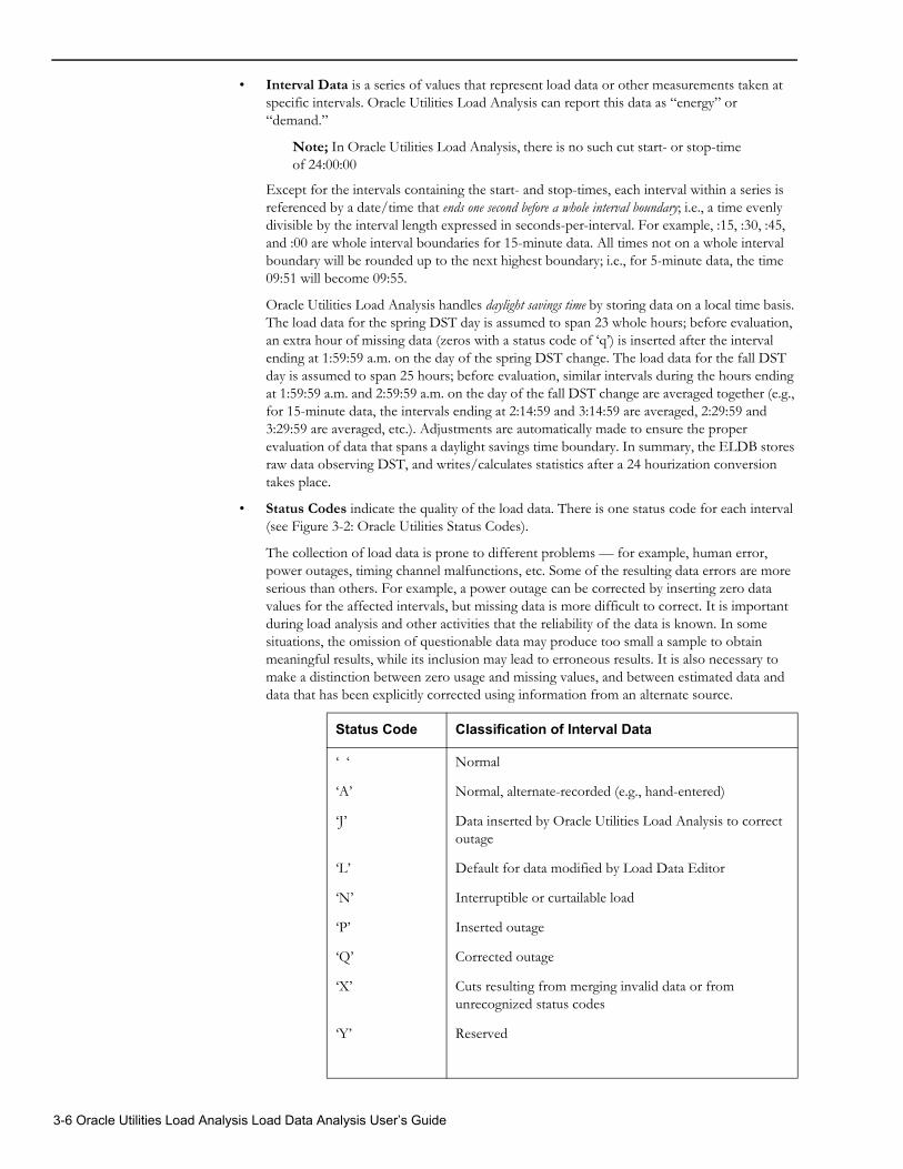
• Interval Data is a series of values that represent load data or other measurements taken at specific intervals. Oracle Utilities Load Analysis can report this data as “energy” or “demand.”
Note; In Oracle Utilities Load Analysis, there is no such cut start- or stop-time of 24:00:00
Except for the intervals containing the start- and stop-times, each interval within a series is referenced by a date/time that ends one second before a whole interval boundary; i.e., a time evenly divisible by the interval length expressed in seconds-per-interval. For example, :15, :30, :45, and :00 are whole interval boundaries for 15-minute data. All times not on a whole interval boundary will be rounded up to the next highest boundary; i.e., for 5-minute data, the time 09:51 will become 09:55.
Oracle Utilities Load Analysis handles daylight savings time by storing data on a local time basis. The load data for the spring DST day is assumed to span 23 whole hours; before evaluation, an extra hour of missing data (zeros with a status code of ‘q’) is inserted after the interval ending at 1:59:59 a.m. on the day of the spring DST change. The load data for the fall DST day is assumed to span 25 hours; before evaluation, similar intervals during the hours ending at 1:59:59 a.m. and 2:59:59 a.m. on the day of the fall DST change are averaged together (e.g., for 15-minute data, the intervals ending at 2:14:59 and 3:14:59 are averaged, 2:29:59 and 3:29:59 are averaged, etc.). Adjustments are automatically made to ensure the proper evaluation of data that spans a daylight savings time boundary. In summary, the ELDB stores raw data observing DST, and writes/calculates statistics after a 24 hourization conversion takes place.
• Status Codes indicate the quality of the load data. There is one status code for each interval (see Figure 3-2: Oracle Utilities Status Codes).
The collection of load data is prone to different problems — for example, human error, power outages, timing channel malfunctions, etc. Some of the resulting data errors are more serious than others. For example, a power outage can be corrected by inserting zero data values for the affected intervals, but missing data is more difficult to correct. It is important during load analysis and other activities that the reliability of the data is known. In some situations, the omission of questionable data may produce too small a sample to obtain meaningful results, while its inclusion may lead to erroneous results. It is also necessary to make a distinction between zero usage and missing values, and between estimated data and data that has been explicitly corrected using information from an alternate source.
Status Code Classification of Interval Data
‘ ‘ Normal
‘A’ Normal, alternate-recorded (e.g., hand-entered)
‘J’ Data inserted by Oracle Utilities Load Analysis to correct outage
‘L’ Default for data modified by Load Data Editor
‘N’ Interruptible or curtailable load
‘P’ Inserted outage
‘Q’ Corrected outage
‘X’ Cuts resulting from merging invalid data or from unrecognized status codes
‘Y’ Reserved
3-6 Oracle Utilities Load Analysis Load Data Analysis User’s Guide
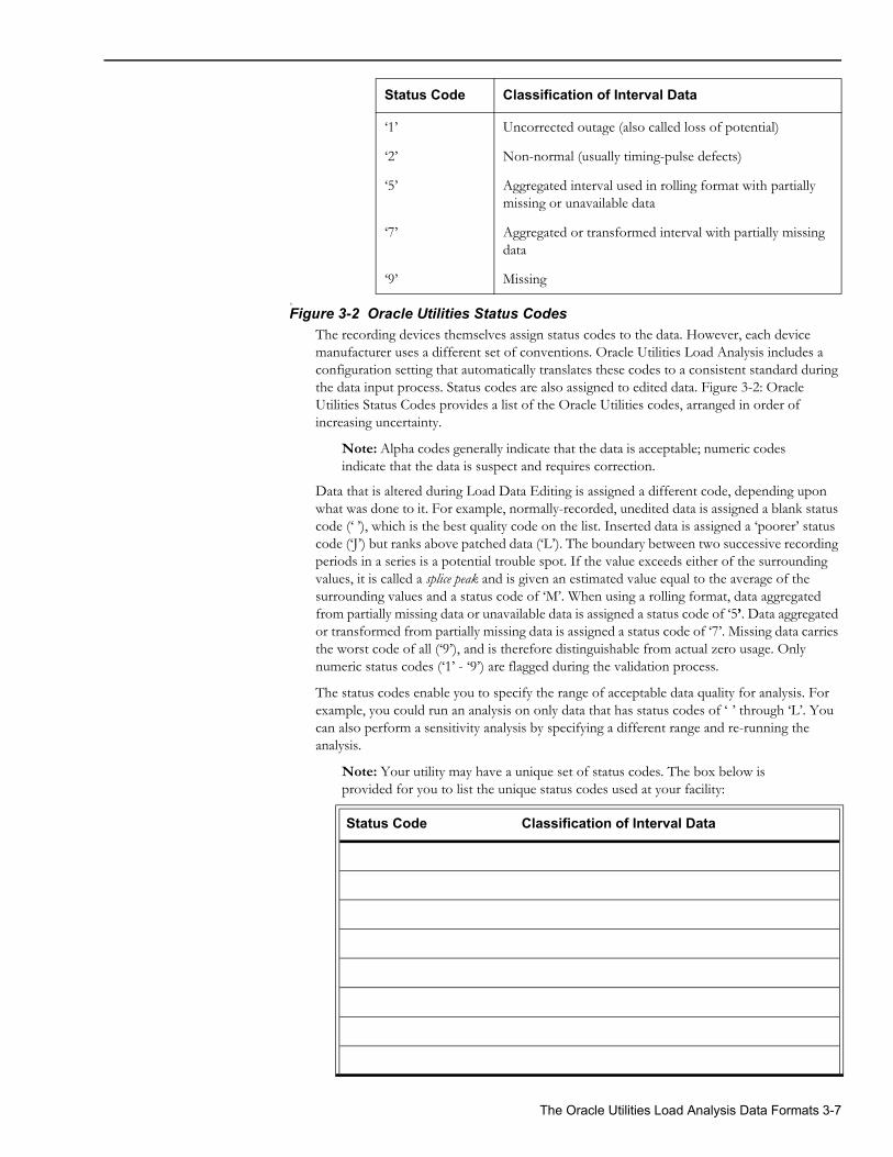
().
Figure 3-2 Oracle Utilities Status CodesThe recording devices themselves assign status codes to the data. However, each device manufacturer uses a different set of conventions. Oracle Utilities Load Analysis includes a configuration setting that automatically translates these codes to a consistent standard during the data input process. Status codes are also assigned to edited data. Figure 3-2: Oracle Utilities Status Codes provides a list of the Oracle Utilities codes, arranged in order of increasing uncertainty.
Note: Alpha codes generally indicate that the data is acceptable; numeric codes indicate that the data is suspect and requires correction.
Data that is altered during Load Data Editing is assigned a different code, depending upon what was done to it. For example, normally-recorded, unedited data is assigned a blank status code (‘ ’), which is the best quality code on the list. Inserted data is assigned a ‘poorer’ status code (‘J’) but ranks above patched data (‘L’). The boundary between two successive recording periods in a series is a potential trouble spot. If the value exceeds either of the surrounding values, it is called a splice peak and is given an estimated value equal to the average of the surrounding values and a status code of ‘M’. When using a rolling format, data aggregated from partially missing data or unavailable data is assigned a status code of ‘5’. Data aggregated or transformed from partially missing data is assigned a status code of ‘7’. Missing data carries the worst code of all (‘9’), and is therefore distinguishable from actual zero usage. Only numeric status codes (‘1’ - ‘9’) are flagged during the validation process.
The status codes enable you to specify the range of acceptable data quality for analysis. For example, you could run an analysis on only data that has status codes of ‘ ’ through ‘L’. You can also perform a sensitivity analysis by specifying a different range and re-running the analysis.
Note: Your utility may have a unique set of status codes. The box below is provided for you to list the unique status codes used at your facility:
‘1’ Uncorrected outage (also called loss of potential)
‘2’ Non-normal (usually timing-pulse defects)
‘5’ Aggregated interval used in rolling format with partially missing or unavailable data
‘7’ Aggregated or transformed interval with partially missing data
‘9’ Missing
Status Code Classification of Interval Data
Status Code Classification of Interval Data
The Oracle Utilities Load Analysis Data Formats 3-7
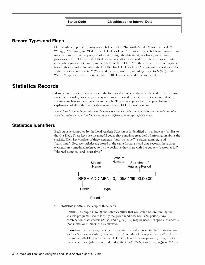
Record Types and FlagsOn records or reports, you may notice fields marked “Internally Valid”, “Externally Valid”, “Merge,” “Archive”, and “Edit”. Oracle Utilities Load Analysis sets these fields automatically and uses them to manage the progress of a cut through the data input, validation, and editing processes in the CLDB and ALDB. They will not affect your work with the analysis subsystem except when you extract data from the ALDB or the CLDB. (See the chapter on extracting data later in this manual.) On cuts in the ELDB, Oracle Utilities Load Analysis automatically sets the External Validation flags to Y (Yes), and the Edit, Archive, and Merge flags to N (No). Only “Active” type records are stored in the ELDB. There is no audit trail in the ELDB.
Statistics RecordsMost often, you will view statistics in the formatted reports produced at the end of the analysis runs. Occasionally, however, you may want to see more detailed information about individual statistics, such as strata population and weight. This section provides a complete list and explanation of all of the data fields contained in an ELDB statistics record.
You will see that statistics records share the same format as load data records. That is why a statistics record is sometimes referred to as a “cut.” However, there are differences in the types of data stored.
Statistics IdentifiersEach statistic computed by the Load Analysis Subsystem is identified by a unique key (similar to the Cut Key). These keys are meaningful codes that contain a great deal of information about the statistic. Each key consists of three elements: “statistic name,” “stratum number,” and “start-time.” Because statistics are stored in the same format as load data records, these three elements are sometimes referred to by the positions they share with the cut key: “customer-id,” “channel-number,” and “start-time.”
• Statistics Name is made up of three parts:
Prefix — a unique 1- to 40-character identifier that you assign before running the analysis program; used to identify the group (and possibly TOU period). Any combination of characters (A - Z) and digits (0 - 9) may be used, but special characters (not a letter or number) are not allowed.
Period — in most cases, this indicates the time period represented by the statistic — such as “average weekday”, “average Friday”, or “day of class peak demand”. This field is automatically filled in by the Oracle Utilities Load Analysis program, using a 2- to 5-character code (which is reproduced in the Oracle Utilities Load Analysis Quick Reference
Status Code Classification of Interval Data
RESH-AD-CMEN, 0, 05/01/99-00:00:00
Prefix Type
Period
StratumNumberStatistic
NameStart time of
Analysis Period
3-8 Oracle Utilities Load Analysis Load Data Analysis User’s Guide
Guide under “Report Qualifiers”). For instance, in the example above, “AD” represents average day.
Type — in most cases, this represents the methodology used to compute the statistic, and the type of statistic, e.g., “Combined Relative Precision” or “Standard Error Combined Ratio Mean KW”. This field is automatically filled in by the Oracle Utilities Load Analysis program using a 4-character code (which is reproduced in the Oracle Utilities Load Analysis Quick Reference Guide under “Statistic Qualifiers”). For instance, in the example above, “CMEN” represents “Combined Ratio Mean KW”. Statistical cuts will have the statistic description in a validation message.
• Stratum Number identifies the group for which the statistic was computed. The value is automatically assigned in the statistics identifier by Oracle Utilities Load Analysis (based on your input in the analysis Control files).
Note: A stratum number of 0 may indicate “Entire Period.”
If there are no strata (such as for sample statistics), Oracle Utilities Load Analysis puts a "0" in the stratum number field.
• Start-time indicates the start-time of the analysis period. It is important to note that, for all statistics, this date and time represent the beginning of the entire period examined in the analysis, not the particular date or date range represented by a specific statistic. For example, if a statistic were computed for the day of class peak during the month of May, the start-time in the identifier would be 05/01/89-00:00:00, even if the class peak occurred on May 7th. This approach is designed to ensure that all statistics for a given analysis period can be identified together. An alternate method of separating and arranging your statistic records is to set up tablesets to specially hold the records. All Analysis programs have the capability to read Interval data from one tableset and write the statistics to another. Both of these tablesets need to be defined on the server as ELDBs.
The conventions for expressing start-times for statistics are the same as for load data records.
The Oracle Utilities Load Analysis Data Formats 3-9
Header and Interval Data for Statistics RecordsEach field is described in detail below and on the following pages. The fields are described in the order in which they appear on the report.
• Statistics Name appears in the field labeled “customer-id”. See the previous page for a further description.
• Stratum Number appears in the field labeled “channel-number”. See the previous page for a further description.
• Start-time represents the beginning of the analysis period.
• Stop-time is the stop time, calculated based on the number of data values (which may or may not represent intervaks) in the record.
• Descriptor is an 80-character field specifying the type of statistic in the report. It is automatically filled in by Oracle Utilities Load Analysis.
• Time span — “Expected” describes the entire period under analysis; “Recorded” describes the time span for the computed statistic.
Note: The number of recorded intervals is the number of intervals or data values that will appear in the second half of the statistics record.
• Seconds/interval is typically the length of each interval. You determine this value before analysis or reporting.
• Population — You enter this value in the Environment File before running the analysis programs.
• Weight — You assign this value before running the analysis programs.
• Number of Time-of-Use periods is automatically filled in by Oracle Utilities Load Analysis.
• Number of Supplied Peaks is automatically filled in by Oracle Utilities Load Analysis.
• UOM stands for “Unit of Measure” and identifies the type of data stored in the interval portion of the record. See Appendix J: Oracle Utilities Unit of Measure Codes for a list of these codes and their meanings.
• Pulse Multiplier and Pulse Offset are shown only for certain load data records; they are not meaningful for statistics.
• Energy is the sum of the interval energies. (If appropriate - please note that this may not be meaningful if the interval data does not represent usage.)
• Sample Titles and Day and Time of Peak for Peak Statistic Records sometimes appear in the Title or Description field. Up to three sample titles or peak times (which you assign before analysis) are stored in this field. These titles appear in reports produced by the Time Series Reporter.
• Edit Trails are not used for statistics records.
• Interval Data — The values reported in this portion of the record have different meanings, depending upon the type of statistics record. For Entire Period and Average Day records, the values represent estimates for the group, interval by interval. For Time-of-Use statistics, the values represent estimates of energy, demand, or load factor by time period.
Note: When viewing reports of interval data, all statistics should be viewed as energy data, not demand data.
• Status Codes — each computed statistic value has a status code of blank (‘ ’). Values that cannot be computed have a value of zero and a status code of ‘9’.
• Flags and record type have no meaning in statistics records.
3-10 Oracle Utilities Load Analysis Load Data Analysis User’s Guide
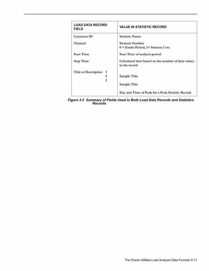
Figure 3-3 Summary of Fields Used in Both Load Data Records and Statistics Records
LOAD DATA RECORD FIELD VALUE IN STATISTIC RECORD
Customer ID Statistic Name
Channel Stratum Number0 = Entire Period, 1= Stratum 1 etc.
Start Time Start Time of analysis period
Stop Time Calculated time based on the number of data values in the record
Title or Description 1 2 3
Sample Title
Sample Title
Day and Time of Peak for a Peak Statistic Record
The Oracle Utilities Load Analysis Data Formats 3-11

3-12 Oracle Utilities Load Analysis Load Data Analysis User’s Guide
Chapter 4Oracle Utilities Load Analysis Mechanics
This chapter is intended primarily for anyone unfamiliar with the basic concepts of input and output files. However, the chapter also defines some important terms unique to Oracle Utilities Load Analysis, such as “Environment files” and “Control files.” Topics covered in this chapter are:
• What Input Files are Used in Oracle Utilities Load Analysis?
• What Output Files Does Oracle Utilities Load Analysis Produce?
• Naming Conventions in Oracle Utilities Load Analysis
• Using the Key Generator Preprocessor in a Control File
• Querying the Database with Embedded Query Statements
Oracle Utilities Load Analysis Mechanics 4-1
Before you begin working with Oracle Utilities Load Analysis, you might want to review some of the basics of working with the programs on your computer system.
You typically accomplish tasks by submitting custom command files or Oracle Utilities Load Analysis “jobs” that run programs. Each program requires input files and produces output files. Output files may be used as the final result (reports, for example), or become input for other programs.
Another way of looking at this is that you can accomplish the tasks by following three main steps:
1. Creating Input Files
2. Running the Program
3. Checking Output Files.
What Input Files are Used in Oracle Utilities Load Analysis?Most Oracle Utilities Load Analysis programs use two types of input files: control files and environment files.
• The Control File typically contains the data to be processed. Queries, customer lists, and lists of keys for load data records are common kinds of control files.
• The Environment File contains your processing instructions to the program. Typically, you select among a set of optional parameters to define the file.
Some programs also use one or more of the following files: Time of Use File, Holiday File, and/or auxiliary database (AXDB). The first two are typically set up at system installation. The AXDB is explained in Chapter 7: Using the Auxiliary Database (AXDB) to Modify Incoming Data (X170, X180).
What Output Files Does Oracle Utilities Load Analysis Produce?Output — the result of running a program — can be new or modified data entered into a tablset, or reports or data files. Aside from special reports, several reports are automatically produced by Oracle Utilities Load Analysis to help you evaluate the success of the program run. (These reports are typically bundled into a single output file called “REPORT.HTML”.)
• The Environment Report describes the processing mode in effect during the program run. Use this report to verify that you entered the correct commands and parameters in the Environment File, and that the defaults used are as intended.
• The Execution Log typically lists data that was altered or created during the program run; it often includes diagnostic messages that alert you to any problems with the input data or the run.
• The Summary usually provides counts of records entered or modified in the tableset as a result of the run.
4-2 Oracle Utilities Load Analysis Load Data Analysis User’s Guide
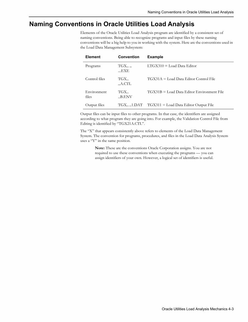
Naming Conventions in Oracle Utilities Load Analysis
Naming Conventions in Oracle Utilities Load AnalysisElements of the Oracle Utilities Load Analysis program are identified by a consistent set of naming conventions. Being able to recognize programs and input files by these naming conventions will be a big help to you in working with the system. Here are the conventions used in the Load Data Management Subsystem:
Output files can be input files to other programs. In that case, the identifiers are assigned according to what program they are going into. For example, the Validation Control File from Editing is identified by “TGX21A.CTL”.
The “X” that appears consistently above refers to elements of the Load Data Management System. The convention for programs, procedures, and files in the Load Data Analysis System uses a “Y” in the same position.
Note: These are the conventions Oracle Corporation assigns. You are not required to use these conventions when executing the programs — you can assign identifiers of your own. However, a logical set of identifiers is useful.
Element Convention Example
Programs TGX_ _ _.EXE
LTGX310 = Load Data Editor
Control files TGX_ _A.CTL
TGX31A = Load Data Editor Control File
Environment files
TGX_ _B.ENV
TGX31B = Load Data Editor Environment File
Output files TGX_ _1.DAT TGX311 = Load Data Editor Output File
Oracle Utilities Load Analysis Mechanics 4-3
Using the Key Generator Preprocessor in a Control File
Using the Key Generator Preprocessor in a Control File Traditionally, using a key generator query (described later) to run a report required submitting two separate jobs. For example, to run the X440 program using a list of generated keys you had to:
1. Submit an X810 Key Generator job.
2. Submit an X440 Summary Reporter job using the results returned from the X810 job.
This example requires the following steps:
1. Create the X810 CTL file.
2. Run the X810 Key Generator.
3. Wait for the job to complete.
4. Copy the contents of the generated output list and paste it into the X440 CTL file.
5. Run the X440 Summary Reporter.
Now you can use the Preprocess Key Generator to consolidate these steps into one job by embedding key generator logic into a control file. Doing so allows you to dynamically create a list of full or partial keys to be used by the program.
For example, you can include the following key generator commands in your X440 control file to run the Summary Reporter on all cuts with a CUSTID that begins with “N”:
L1: SUBSTR(CUSTID,1,1) = 'N' T(PRINT 1) F(NEXT)
FORMATS:1: TRIM(CUSTID) ', ' TRIM(CHANNEL)
Note:
For programs that can run against multiple tablesets, the preprocessor will only run against the primary tableset selected (CLDB if selected, ALDB if no CLDB is available).
If an error occurs during the key generator query process, the job will be aborted with return code 99. Key generator outputs (such as sysprints and reports) will remain in the job output folder. You can use these files to troubleshoot the error that occurred.
For more information about the key generator program see Chapter 15: Key Generator — A Shortcut for Creating Input Files and Reports.
Preprocessing OptionsYou can use the following optional features with the key generator preprocessor.
Keys List (Optional)The KEYSLIST command provides the same functionality as the optional keys list file used by the key generator program. This command allows you to filter the results of the pre-processing query to a select subset of keys or limit the list of cuts scanned by the key generator.
To supply an optional key generator keys list (reducing the runtime significantly), enter the following statement at the end of your pre-process control file:
KEYSLIST:
Following the KEYSLIST statement, supply your list of keys (full, partial, or an embedded Query (@SELECT ...) in the subsequent lines using the following syntax:
KEYSLIST:custid channel [start-time] (0r an embedded Query statement)
4-4 Oracle Utilities Load Analysis Load Data Analysis User’s Guide
Using the Key Generator Preprocessor in a Control File
Example CTL file with KEYSLIST statement:
L1: SUBSTR(CUSTID,1,1) = 'N' T(PRINT 1) F(NEXT)
FORMATS:1: TRIM(CUSTID) ', ' TRIM(CHANNEL)
KEYSLIST:N1723, 1N1725, 1
Example using Embedded Query Statement:
KEYSLIST:@SELECT FKEY WHERE CUSTID LIKE 'N%'
Environment File (Optional)The Preprocess Key Generator uses the tgx81b.env file in the COMMON/DATA directory as a default environment file. If this file is not found, the key generator will create one with the following default value:
PRINT ECONOMY
You can override this setting to provide a custom environment file by using the following statement at the end of your pre-processing control file.
ENV:
Following the ENV statement, enter your environment commands. The following is an example:
/* FIND CUTS WITH MORE THAN 1 EDIT (EACH EDIT PRODUCES 2 TRAILS)L1: TRAILCT > 2 T(PRINT 1) F(NEXT)
FORMATS:1: TRIM(CUSTID) ', ' TRIM(CHANNEL) ', ' TRIM(START)
KEYSLIST:@SELECT FKEY WHERE CUSTID LIKE 'N%'
ENV:TRAILSPRINT ECO
Supported ProgramsThe following Load Analysis programs support the Preprocess Key Generator:
• X210 Cut Series Validation
• X310 Load Data Editor (CLDB)
• X410 Load Data Reporter
• X430 Totalizing Reporter
• X440 Summary Reporter
• X470 Late Cut Report
• X480 Validation Statistics Reporter
Oracle Utilities Load Analysis Mechanics 4-5
Using the Key Generator Preprocessor in a Control File
• X490 Cut Series gap Reporter
• X530 Cut Series Overlap reporter
• X720 Direct Output (CLDB)
• Y230 Billed Energy Program
• Y240 Load Data Extraction
• Y310 Standard Load Data Analysis
• Y320 Aggregate Load Analysis
• Y330 Ratio Analysis
• Y350 Domain Analysis MPU
• Y360 Domains Analysis Ratio
• Y370 Individual Customer Analysis
• Y380 100% Sample Analysis
• Y410 Time Series Reporter
• Y620 Load Data Transformation
• Y630 Load Data Editor (ELDB)
• Y720 Direct Output (ELDB)
• Q91C Copy Cuts
• Q91D Delete Cuts
• Q91M Move Cuts
4-6 Oracle Utilities Load Analysis Load Data Analysis User’s Guide
Querying the Database with Embedded Query Statements
Querying the Database with Embedded Query StatementsThe key generator has traditionally been used to query a tableset to create a list of cuts or cut series for input into programs. The key generator works well for complicated query logic, but it can be inefficient when used to search for cuts in a large tableset. For that situation, a better way to query the database is with embedded query statements.
Query statements can be embedded in an input control or key list file for programs that take a list of cuts or cut series as input. The query is used to query the tableset and return a list of cut or cut series before the a program is run. The control file or key list file that contains embedded query will have the query statements replaced with the results of the query before the main program is processed.
Syntax for Embedded Query StatementsAll embedded query statements are identified by the keyword @SELECT and use the following syntax:
@SELECT selectFields WHERE whereConditions[KEYSLIST:]
Where:
selectFields are a comma-separated list of cut values to return. See Selection Field Names for a list of available field names.
whereConditions are a set of conditions from which to use as criteria for selection. The where conditions have the following format:
FIELD comparison-operator VALUE
Where:
FIELD specifies the field name which will be the target of the selection criteria. See Selection Field Names for a list of available field names.
comparison-operator specifies the logic to use for the comparison. See Comparison Operators for a list of available operators.
VALUE specifies a value to compare the field to. Values can be of type string, numeric, or Boolean.
Values should be in the following formats:
• String data types must be enclosed in single quotes ('example').
• Boolean values must be 'YES', 'Y', 'TRUE', 'NO', 'N', or 'FALSE'.
• Numeric values (NUM values) must be numeric with no plus (+) signs. They can either be in single quotes or not.
• Dates must to follow the standard Oracle Utilities Load Analysis convention (MM/DD/YY-HH:MM:SS or MM/DD/YY). They can either be in single quotes or not.
• Lists need to be enclosed in parentheses and values separated by commas. For example:
CUSTID IN ('N1723', 'N1724')
The following is an example of an embedded query statement:
@SELECT CUSTID, CHANNEL WHERE CHANNEL = 1
You can set multiple where conditions by joining them using AND and OR statements. Sets of conditions can be grouped together by enclosing them in parenthesis "()".
Oracle Utilities Load Analysis Mechanics 4-7
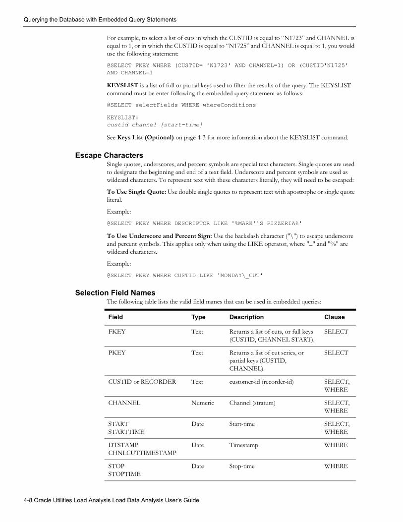
Querying the Database with Embedded Query Statements
For example, to select a list of cuts in which the CUSTID is equal to “N1723” and CHANNEL is equal to 1, or in which the CUSTID is equal to “N1725” and CHANNEL is equal to 1, you would use the following statement:
@SELECT FKEY WHERE (CUSTID= 'N1723' AND CHANNEL=1) OR (CUSTID'N1725' AND CHANNEL=1
KEYSLIST is a list of full or partial keys used to filter the results of the query. The KEYSLIST command must be enter following the embedded query statement as follows:
@SELECT selectFields WHERE whereConditionsKEYSLIST:custid channel [start-time]
See Keys List (Optional) on page 4-3 for more information about the KEYSLIST command.
Escape CharactersSingle quotes, underscores, and percent symbols are special text characters. Single quotes are used to designate the beginning and end of a text field. Underscore and percent symbols are used as wildcard characters. To represent text with these characters literally, they will need to be escaped:
To Use Single Quote: Use double single quotes to represent text with apostrophe or single quote literal.
Example:
@SELECT PKEY WHERE DESCRIPTOR LIKE '%MARK''S PIZZERIA%'
To Use Underscore and Percent Sign: Use the backslash character ("\") to escape underscore and percent symbols. This applies only when using the LIKE operator, where "_" and "%" are wildcard characters.
Example:
@SELECT PKEY WHERE CUSTID LIKE 'MONDAY\_CUT'
Selection Field NamesThe following table lists the valid field names that can be used in embedded queries:
Field Type Description Clause
FKEY Text Returns a list of cuts, or full keys (CUSTID, CHANNEL START).
SELECT
PKEY Text Returns a list of cut series, or partial keys (CUSTID, CHANNEL).
SELECT
CUSTID or RECORDER Text customer-id (recorder-id) SELECT, WHERE
CHANNEL Numeric Channel (stratum) SELECT, WHERE
STARTSTARTTIME
Date Start-time SELECT, WHERE
DTSTAMPCHNLCUTTIMESTAMP
Date Timestamp WHERE
STOPSTOPTIME
Date Stop-time WHERE
4-8 Oracle Utilities Load Analysis Load Data Analysis User’s Guide
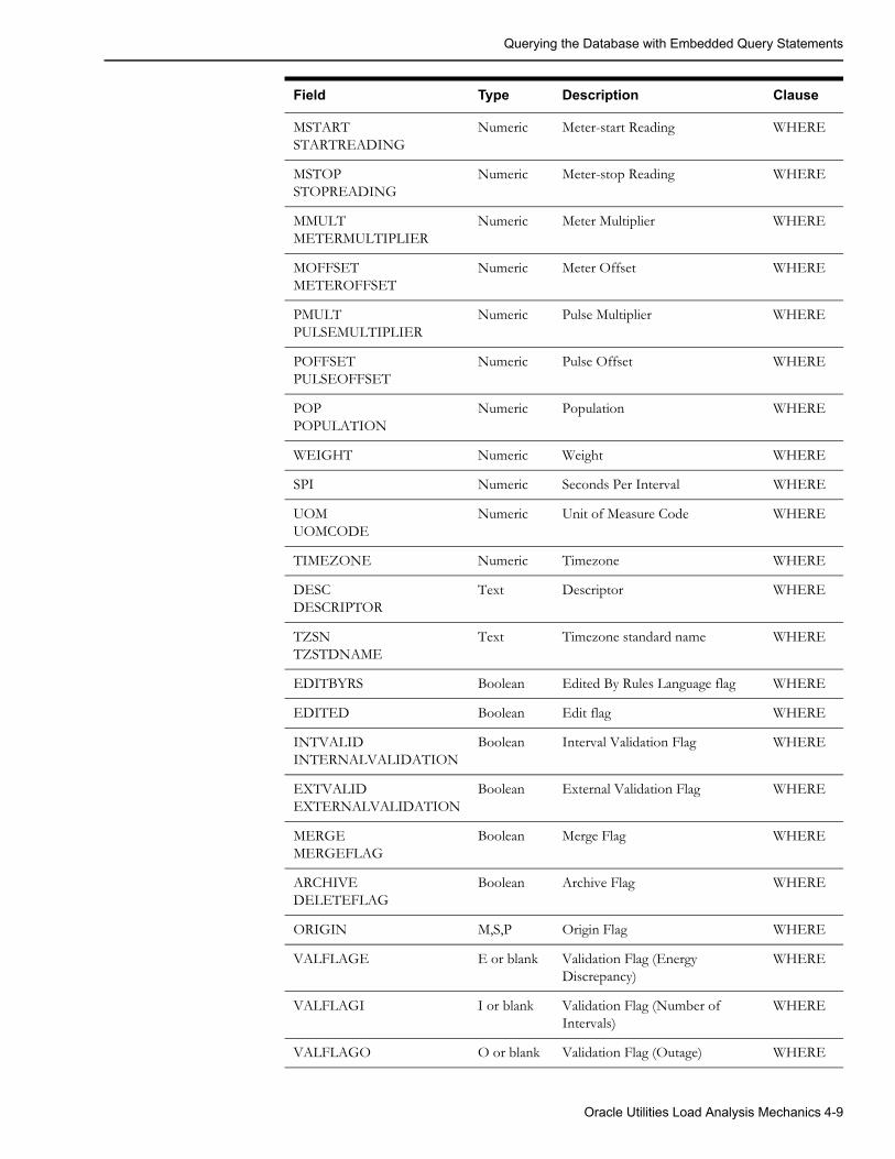
Querying the Database with Embedded Query Statements
MSTARTSTARTREADING
Numeric Meter-start Reading WHERE
MSTOPSTOPREADING
Numeric Meter-stop Reading WHERE
MMULTMETERMULTIPLIER
Numeric Meter Multiplier WHERE
MOFFSETMETEROFFSET
Numeric Meter Offset WHERE
PMULTPULSEMULTIPLIER
Numeric Pulse Multiplier WHERE
POFFSETPULSEOFFSET
Numeric Pulse Offset WHERE
POPPOPULATION
Numeric Population WHERE
WEIGHT Numeric Weight WHERE
SPI Numeric Seconds Per Interval WHERE
UOMUOMCODE
Numeric Unit of Measure Code WHERE
TIMEZONE Numeric Timezone WHERE
DESCDESCRIPTOR
Text Descriptor WHERE
TZSNTZSTDNAME
Text Timezone standard name WHERE
EDITBYRS Boolean Edited By Rules Language flag WHERE
EDITED Boolean Edit flag WHERE
INTVALIDINTERNALVALIDATION
Boolean Interval Validation Flag WHERE
EXTVALIDEXTERNALVALIDATION
Boolean External Validation Flag WHERE
MERGEMERGEFLAG
Boolean Merge Flag WHERE
ARCHIVEDELETEFLAG
Boolean Archive Flag WHERE
ORIGIN M,S,P Origin Flag WHERE
VALFLAGE E or blank Validation Flag (Energy Discrepancy)
WHERE
VALFLAGI I or blank Validation Flag (Number of Intervals)
WHERE
VALFLAGO O or blank Validation Flag (Outage) WHERE
Field Type Description Clause
Oracle Utilities Load Analysis Mechanics 4-9
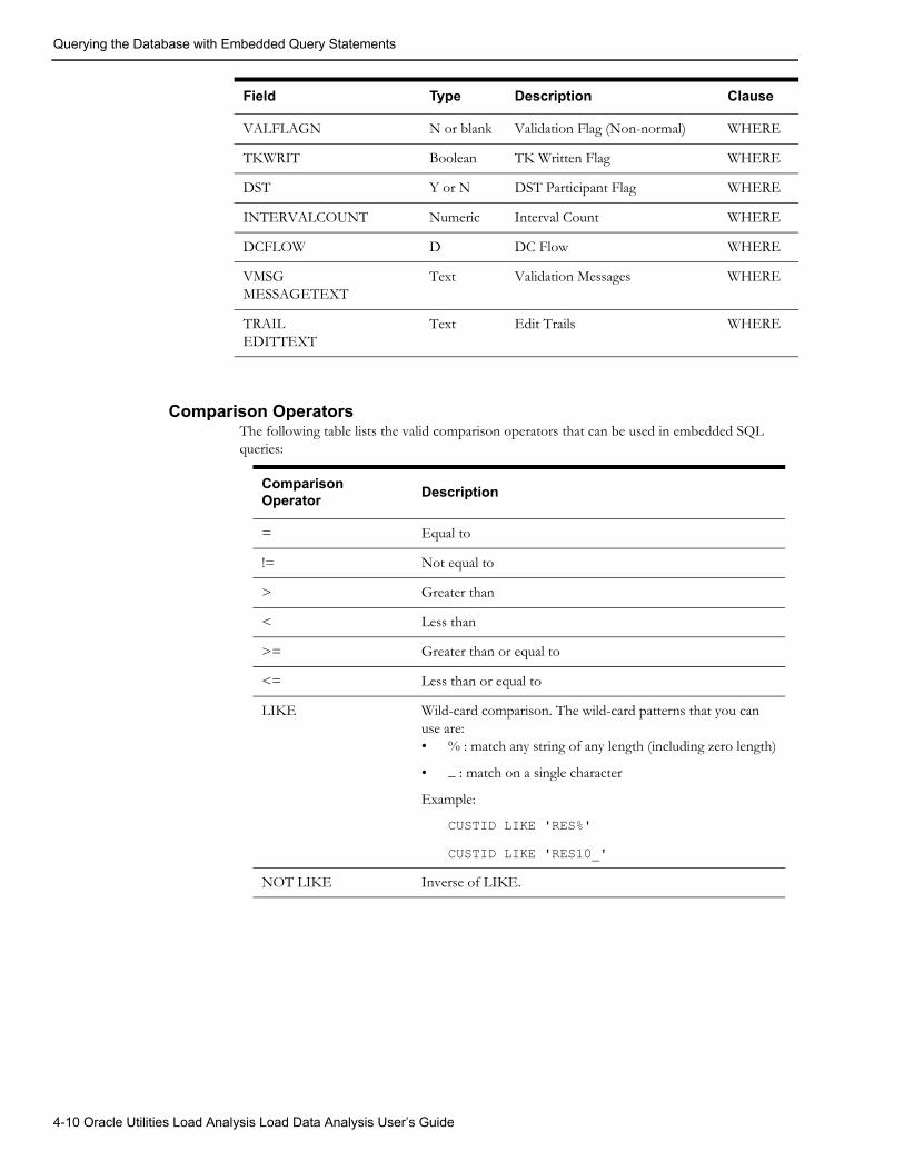
Querying the Database with Embedded Query Statements
Comparison OperatorsThe following table lists the valid comparison operators that can be used in embedded SQL queries:
VALFLAGN N or blank Validation Flag (Non-normal) WHERE
TKWRIT Boolean TK Written Flag WHERE
DST Y or N DST Participant Flag WHERE
INTERVALCOUNT Numeric Interval Count WHERE
DCFLOW D DC Flow WHERE
VMSGMESSAGETEXT
Text Validation Messages WHERE
TRAILEDITTEXT
Text Edit Trails WHERE
Field Type Description Clause
Comparison Operator Description
= Equal to
!= Not equal to
> Greater than
< Less than
>= Greater than or equal to
<= Less than or equal to
LIKE Wild-card comparison. The wild-card patterns that you can use are:• % : match any string of any length (including zero length)
• _ : match on a single character
Example:
CUSTID LIKE 'RES%'CUSTID LIKE 'RES10_'
NOT LIKE Inverse of LIKE.
4-10 Oracle Utilities Load Analysis Load Data Analysis User’s Guide
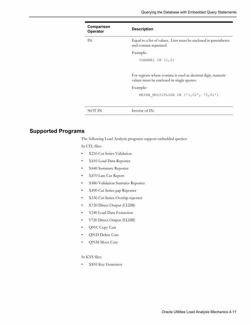
Querying the Database with Embedded Query Statements
Supported ProgramsThe following Load Analysis programs support embedded queries:
In CTL files:
• X210 Cut Series Validation
• X410 Load Data Reporter
• X440 Summary Reporter
• X470 Late Cut Report
• X480 Validation Statistics Reporter
• X490 Cut Series gap Reporter
• X530 Cut Series Overlap reporter
• X720 Direct Output (CLDB)
• Y240 Load Data Extraction
• Y720 Direct Output (ELDB)
• Q91C Copy Cuts
• Q91D Delete Cuts
• Q91M Move Cuts
In KYS files:
• X810 Key Generator
IN Equal to a list of values. Lists must be enclosed in parentheses and comma separated.
Example:
CHANNEL IN (1,2)
For regions where comma is used as decimal digit, numeric values must be enclosed in single quotes.
Example:
METER_MULTIPLIER IN ('1,02', '2,01')
NOT IN Inverse of IN.
Comparison Operator Description
Oracle Utilities Load Analysis Mechanics 4-11
Querying the Database with Embedded Query Statements
Custom VariablesCustom Key Generator variables can also be used in embedded query statements. They can be referenced just like any other variable with certain limitations (see below).
Example:
@SELECT FKEY WHERE RATE = 'N1';
See oula_server.cfg.xml on page 1-14 in the Oracle Utilities Load Analysis Configuration Guide for more information about configuring custom Key Generator variables.
Limitations1. Certain operators cannot work with custom variables. The operator must be one of "=", "!=",
" LIKE " and " NOT LIKE ". For example, the following embedded query would be invalid:
@SELECT FKEY WHERE RATE IN ('R1', 'N1');@SELECT FKEY WHERE RATE > '01';
2. The length of the compare value cannot EXCEED the length of custom variable. For example, if a custom field is defined with a length of 2, compare value cannot exceed 2 characters in length. For example, the following query would be invalid since RATE is defined with LENGTH=2:
@SELECT FKEY WHERE RATE = 'N2024';
3. Multiple wild cards (%) are not allowed. Custom fields do not work with more than one wild card (%) in the compare value. For example, the following embedded query would be invalid:
@SELECT FKEY WHERE RATE LIKE '%N%';
4-12 Oracle Utilities Load Analysis Load Data Analysis User’s Guide
Chapter 5Getting Data into the Extracted Load Database
(Y130, Y220, Y240)
The previous chapters explained the “big picture” of what Oracle Utilities Load Analysis does and why. The remainder of this guide will look more closely at each of the most commonly used procedures in the Load Data Analysis Subsystem.
This chapter describes the first step in working with the subsystem — getting the necessary data organized and input to the Extracted Load Database (ELDB). This chapter focuses on the program most commonly used for this purpose — ALDB/CLDB/ELDB Load Data Extraction (Y240). Two alternative programs, Manual Entry (ELDB) (Y220) and Direct and Production Input (ELDB) (Y130, Y131), are also described briefly. Topics covered are:
• What Does ALDB/CLDB/ELDB Extraction Do?
• Deciding Whether to Extract Data from the ALDB, CLDB or ELDB
• Establishing Guidelines for Data Extraction
• Record Flags and Validation Tests — Oracle Utilities Load Analysis “Quality Control” Mechanisms
• Steps for Using the ALDB/CLDB/ELDB Extraction Program (Y240)
Getting Data into the Extracted Load Database (Y130, Y220, Y240) 5-1
The first step in the analysis process is to put the load data to be analyzed into the Extracted Load Database (ELDB) — the working area for the Load Data Analysis Subsystem. Three programs are available for this purpose:
• ALDB/CLDB /ELDB Load Data Extraction (Y240) — extracts data from other Oracle Utilities Load Analysis databases — the Archive Load Database (ALDB), the Current Load Database (CLDB), or both. This is the recommended method, and is described in detail in this chapter.
Note: This program supports embedded SQL commands. See Querying the Database with Embedded Query Statements on page 4-7 for more information. The program supports pre-process key generator. See Using the Key Generator Preprocessor in a Control File on page 4-4 for more information.
• Manual Entry (Y220) — inputs manually created files to the ELDB. You would typically use this program to input data that does not already exist in electronic media, or is such a small amount that it’s actually quickest to input by hand. See the Oracle Utilities Load Analysis Load Data Management User’s Guide for instructions.
• Direct and Production Input (Y130, Y131) — reads load data from an input file directly into the ELDB. This procedure is identical to the Direct and Production Input programs described in the Oracle Utilities Load Analysis Load Data Management User’s Guide, with the following exception:
• Because the input data is assumed to be accurate, this procedure does not include Validation, and the Load Data Reporter Exception Report is not produced (should include the VALID option in Environment File).
Because this approach bypasses the validation checks that have been designed to help ensure data quality, it is not recommended unless you are absolutely certain that the data is accurate. Otherwise, you should use X110/X111 to input the data to the CLDB, then extract it using Y240 after it has passed all validation tests. (See Chapter 6, “Entering and Validating Data Using the Production Input, Direct Input, or Load Data Input Programs,” in the Oracle Utilities Load Analysis Load Data Management User’s Guide, for details.)
What Does ALDB/CLDB/ELDB Extraction Do?Load Data Extraction (see Figure 5-1: ALDB/CLDB/ELDB Extraction) takes a copy of load data from the ALDB, CLDB, and ELDB or all and inputs it to an ELDB, where you can apply any of several Oracle Utilities Load Analysis Analysis programs to it. You can extract data for any subset of customers over any calendar period that exists in the ALDB, ELDB and/or CLDB. The program automatically combines duplicate or conflicting data according to a prescribed set of rules, creating a single record at a uniform frequency and unit of measure for each customer.
)
CLDB
ALDB
ELDBValidate
Extraction
AnalyzeExtraction
5-2 Oracle Utilities Load Analysis Load Data Analysis User’s Guide
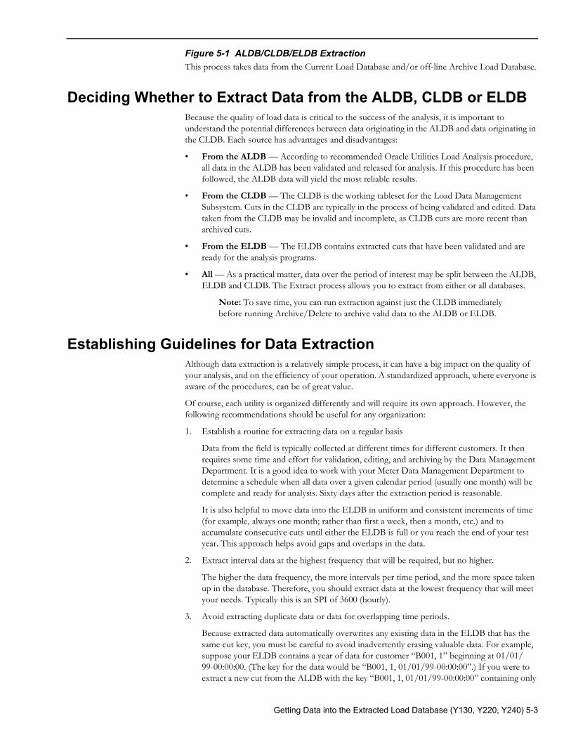
Figure 5-1 ALDB/CLDB/ELDB ExtractionThis process takes data from the Current Load Database and/or off-line Archive Load Database.
Deciding Whether to Extract Data from the ALDB, CLDB or ELDBBecause the quality of load data is critical to the success of the analysis, it is important to understand the potential differences between data originating in the ALDB and data originating in the CLDB. Each source has advantages and disadvantages:
• From the ALDB — According to recommended Oracle Utilities Load Analysis procedure, all data in the ALDB has been validated and released for analysis. If this procedure has been followed, the ALDB data will yield the most reliable results.
• From the CLDB — The CLDB is the working tableset for the Load Data Management Subsystem. Cuts in the CLDB are typically in the process of being validated and edited. Data taken from the CLDB may be invalid and incomplete, as CLDB cuts are more recent than archived cuts.
• From the ELDB — The ELDB contains extracted cuts that have been validated and are ready for the analysis programs.
• All — As a practical matter, data over the period of interest may be split between the ALDB, ELDB and CLDB. The Extract process allows you to extract from either or all databases.
Note: To save time, you can run extraction against just the CLDB immediately before running Archive/Delete to archive valid data to the ALDB or ELDB.
Establishing Guidelines for Data ExtractionAlthough data extraction is a relatively simple process, it can have a big impact on the quality of your analysis, and on the efficiency of your operation. A standardized approach, where everyone is aware of the procedures, can be of great value.
Of course, each utility is organized differently and will require its own approach. However, the following recommendations should be useful for any organization:
1. Establish a routine for extracting data on a regular basis
Data from the field is typically collected at different times for different customers. It then requires some time and effort for validation, editing, and archiving by the Data Management Department. It is a good idea to work with your Meter Data Management Department to determine a schedule when all data over a given calendar period (usually one month) will be complete and ready for analysis. Sixty days after the extraction period is reasonable.
It is also helpful to move data into the ELDB in uniform and consistent increments of time (for example, always one month; rather than first a week, then a month, etc.) and to accumulate consecutive cuts until either the ELDB is full or you reach the end of your test year. This approach helps avoid gaps and overlaps in the data.
2. Extract interval data at the highest frequency that will be required, but no higher.
The higher the data frequency, the more intervals per time period, and the more space taken up in the database. Therefore, you should extract data at the lowest frequency that will meet your needs. Typically this is an SPI of 3600 (hourly).
3. Avoid extracting duplicate data or data for overlapping time periods.
Because extracted data automatically overwrites any existing data in the ELDB that has the same cut key, you must be careful to avoid inadvertently erasing valuable data. For example, suppose your ELDB contains a year of data for customer “B001, 1” beginning at 01/01/99-00:00:00. (The key for the data would be “B001, 1, 01/01/99-00:00:00”.) If you were to extract a new cut from the ALDB with the key “B001, 1, 01/01/99-00:00:00” containing only
Getting Data into the Extracted Load Database (Y130, Y220, Y240) 5-3
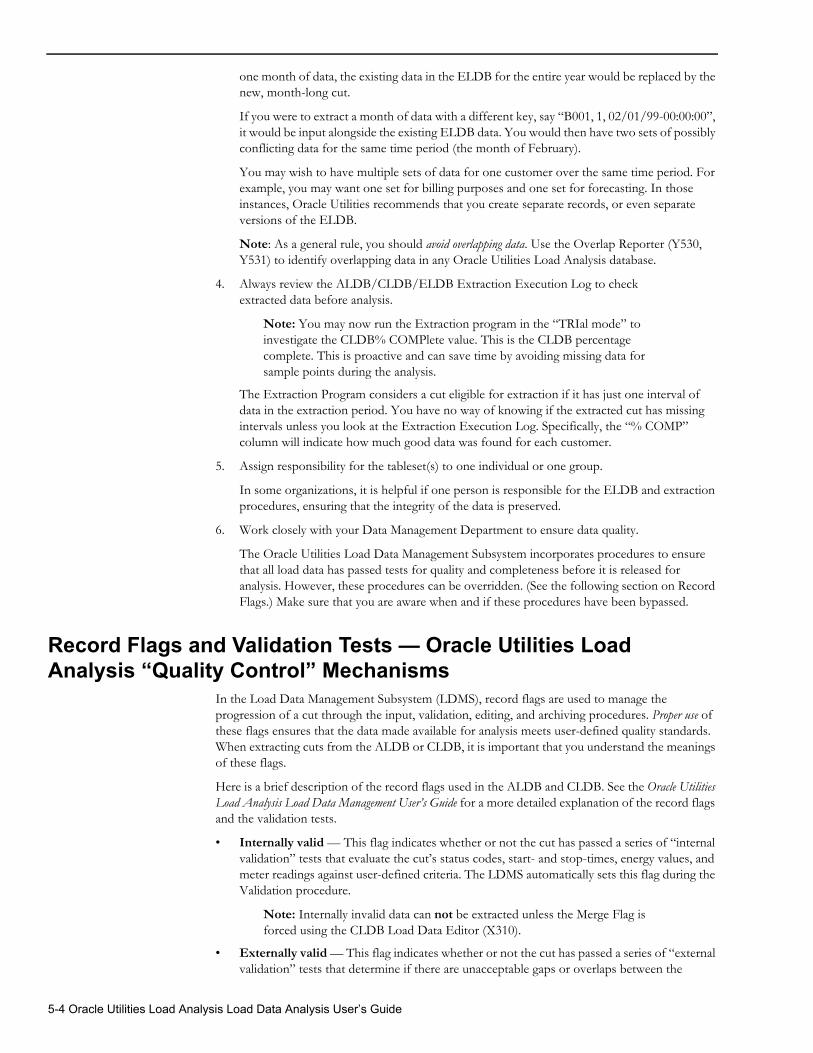
one month of data, the existing data in the ELDB for the entire year would be replaced by the new, month-long cut.
If you were to extract a month of data with a different key, say “B001, 1, 02/01/99-00:00:00”, it would be input alongside the existing ELDB data. You would then have two sets of possibly conflicting data for the same time period (the month of February).
You may wish to have multiple sets of data for one customer over the same time period. For example, you may want one set for billing purposes and one set for forecasting. In those instances, Oracle Utilities recommends that you create separate records, or even separate versions of the ELDB.
Note: As a general rule, you should avoid overlapping data. Use the Overlap Reporter (Y530, Y531) to identify overlapping data in any Oracle Utilities Load Analysis database.
4. Always review the ALDB/CLDB/ELDB Extraction Execution Log to checkextracted data before analysis.
Note: You may now run the Extraction program in the “TRIal mode” to investigate the CLDB% COMPlete value. This is the CLDB percentage complete. This is proactive and can save time by avoiding missing data for sample points during the analysis.
The Extraction Program considers a cut eligible for extraction if it has just one interval of data in the extraction period. You have no way of knowing if the extracted cut has missing intervals unless you look at the Extraction Execution Log. Specifically, the “% COMP” column will indicate how much good data was found for each customer.
5. Assign responsibility for the tableset(s) to one individual or one group.
In some organizations, it is helpful if one person is responsible for the ELDB and extraction procedures, ensuring that the integrity of the data is preserved.
6. Work closely with your Data Management Department to ensure data quality.
The Oracle Utilities Load Data Management Subsystem incorporates procedures to ensure that all load data has passed tests for quality and completeness before it is released for analysis. However, these procedures can be overridden. (See the following section on Record Flags.) Make sure that you are aware when and if these procedures have been bypassed.
Record Flags and Validation Tests — Oracle Utilities Load Analysis “Quality Control” Mechanisms
In the Load Data Management Subsystem (LDMS), record flags are used to manage the progression of a cut through the input, validation, editing, and archiving procedures. Proper use of these flags ensures that the data made available for analysis meets user-defined quality standards. When extracting cuts from the ALDB or CLDB, it is important that you understand the meanings of these flags.
Here is a brief description of the record flags used in the ALDB and CLDB. See the Oracle Utilities Load Analysis Load Data Management User’s Guide for a more detailed explanation of the record flags and the validation tests.
• Internally valid — This flag indicates whether or not the cut has passed a series of “internal validation” tests that evaluate the cut’s status codes, start- and stop-times, energy values, and meter readings against user-defined criteria. The LDMS automatically sets this flag during the Validation procedure.
Note: Internally invalid data can not be extracted unless the Merge Flag is forced using the CLDB Load Data Editor (X310).
• Externally valid — This flag indicates whether or not the cut has passed a series of “external validation” tests that determine if there are unacceptable gaps or overlaps between the
5-4 Oracle Utilities Load Analysis Load Data Analysis User’s Guide
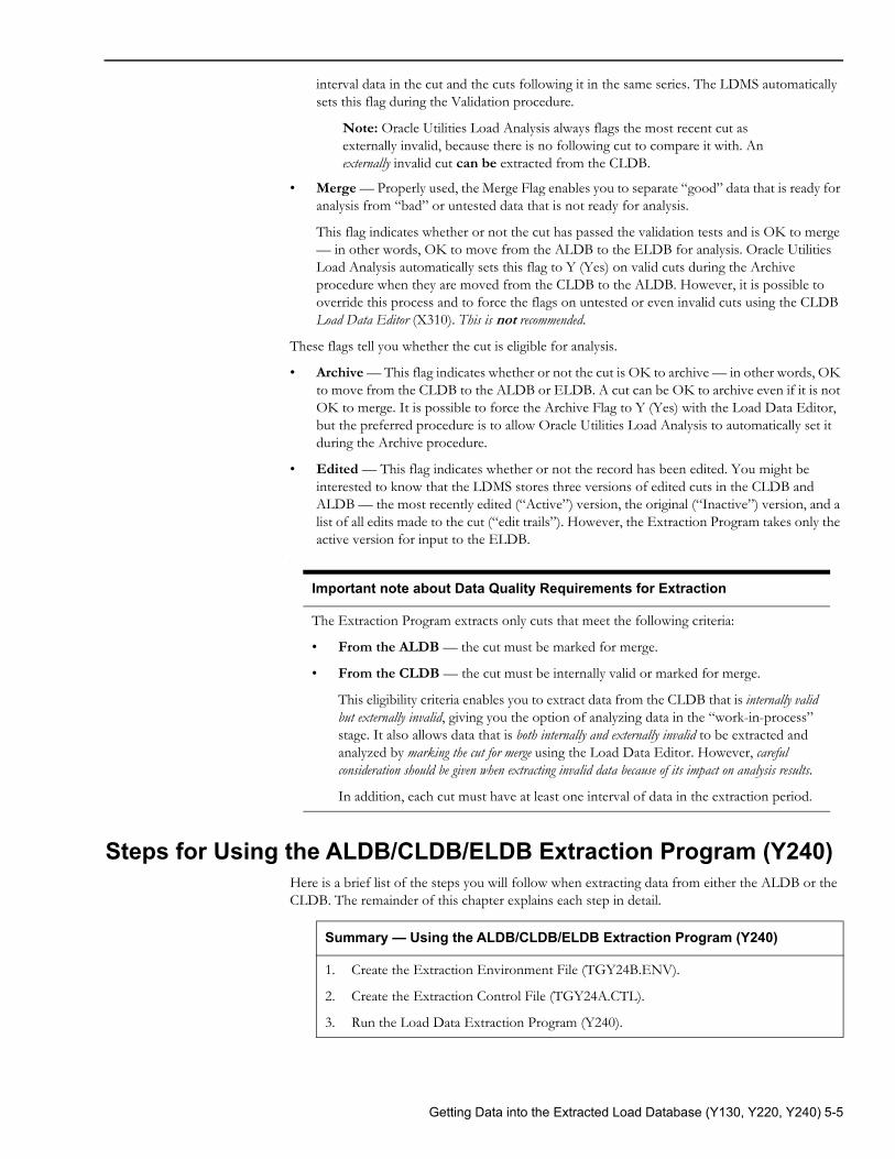
interval data in the cut and the cuts following it in the same series. The LDMS automatically sets this flag during the Validation procedure.
Note: Oracle Utilities Load Analysis always flags the most recent cut as externally invalid, because there is no following cut to compare it with. An externally invalid cut can be extracted from the CLDB.
• Merge — Properly used, the Merge Flag enables you to separate “good” data that is ready for analysis from “bad” or untested data that is not ready for analysis.
This flag indicates whether or not the cut has passed the validation tests and is OK to merge — in other words, OK to move from the ALDB to the ELDB for analysis. Oracle Utilities Load Analysis automatically sets this flag to Y (Yes) on valid cuts during the Archive procedure when they are moved from the CLDB to the ALDB. However, it is possible to override this process and to force the flags on untested or even invalid cuts using the CLDB Load Data Editor (X310). This is not recommended.
These flags tell you whether the cut is eligible for analysis.
• Archive — This flag indicates whether or not the cut is OK to archive — in other words, OK to move from the CLDB to the ALDB or ELDB. A cut can be OK to archive even if it is not OK to merge. It is possible to force the Archive Flag to Y (Yes) with the Load Data Editor, but the preferred procedure is to allow Oracle Utilities Load Analysis to automatically set it during the Archive procedure.
• Edited — This flag indicates whether or not the record has been edited. You might be interested to know that the LDMS stores three versions of edited cuts in the CLDB and ALDB — the most recently edited (“Active”) version, the original (“Inactive”) version, and a list of all edits made to the cut (“edit trails”). However, the Extraction Program takes only the active version for input to the ELDB.
.
Steps for Using the ALDB/CLDB/ELDB Extraction Program (Y240)Here is a brief list of the steps you will follow when extracting data from either the ALDB or the CLDB. The remainder of this chapter explains each step in detail.
Important note about Data Quality Requirements for Extraction
The Extraction Program extracts only cuts that meet the following criteria:
• From the ALDB — the cut must be marked for merge.
• From the CLDB — the cut must be internally valid or marked for merge.
This eligibility criteria enables you to extract data from the CLDB that is internally valid but externally invalid, giving you the option of analyzing data in the “work-in-process” stage. It also allows data that is both internally and externally invalid to be extracted and analyzed by marking the cut for merge using the Load Data Editor. However, careful consideration should be given when extracting invalid data because of its impact on analysis results.
In addition, each cut must have at least one interval of data in the extraction period.
Summary — Using the ALDB/CLDB/ELDB Extraction Program (Y240)
1. Create the Extraction Environment File (TGY24B.ENV).
2. Create the Extraction Control File (TGY24A.CTL).
3. Run the Load Data Extraction Program (Y240).
Getting Data into the Extracted Load Database (Y130, Y220, Y240) 5-5
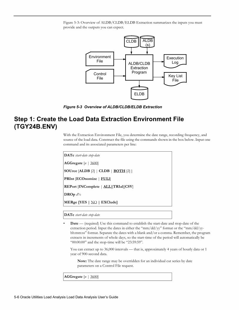
Figure 5-3: Overview of ALDB/CLDB/ELDB Extraction summarizes the inputs you must provide and the outputs you can expect.
Figure 5-3 Overview of ALDB/CLDB/ELDB Extraction
Step 1: Create the Load Data Extraction Environment File (TGY24B.ENV)
With the Extraction Environment File, you determine the date range, recording frequency, and source of the load data. Construct the file using the commands shown in the box below. Input one command and its associated parameters per line:
• Date — (required) Use this command to establish the start-date and stop-date of the extraction period. Input the dates in either the “mm/dd/yy” format or the “mm/dd/yy-hh:mm:ss” format. Separate the dates with a blank and/or a comma. Remember, the program extracts in increments of whole days, so the start-time of the period will automatically be “00:00:00” and the stop-time will be “23:59:59”.
You can extract up to 36,000 intervals — that is, approximately 4 years of hourly data or 1 year of 900-second data.
Note: The date range may be overridden for an individual cut series by dateparameters on a Control File request.
ALDB(s)
ControlFile
EnvironmentFile ALDB/CLDB
ExtractionProgram
ExecutionLog
CLDB
ELDB
Key ListFile
DATe start-date stop-date
AGGregate [n | 3600]
SOUrce [ALDB [2] | CLDB | BOTH [2] ]
PRInt [ECOnomize | FULl]
REPort [INComplete | ALL][TRIal][CSV]
DROp d%
MERge [YES | NO | EXClude]
DATe start-date stop-date
AGGregate [n | 3600]
5-6 Oracle Utilities Load Analysis Load Data Analysis User’s Guide
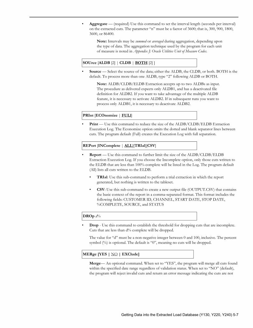
• Aggregate — (required) Use this command to set the interval length (seconds per interval) on the extracted cuts. The parameter “n” must be a factor of 3600; that is, 300, 900, 1800, 3600, or 86400.
Note: Intervals may be summed or averaged during aggregation, depending upon the type of data. The aggregation technique used by the program for each unit of measure is noted in Appendix J: Oracle Utilities Unit of Measure Codes.
• Source — Select the source of the data; either the ALDB, the CLDB, or both. BOTH is the default. To process more than one ALDB, type “2” following ALDB or BOTH.
Note: ALDB/CLDB/ELDB Extraction accepts up to two ALDBs as input. The procedure as delivered expects only ALDB1, and has a deactivated file definition for ALDB2. If you want to take advantage of the multiple ALDB feature, it is necessary to activate ALDB2. If in subsequent runs you want to process only ALDB1, it is necessary to deactivate ALDB2.
• Print — Use this command to reduce the size of the ALDB/CLDB/ELDB Extraction Execution Log. The Economize option omits the dotted and blank separator lines between cuts. The program default (Full) creates the Execution Log with full separation.
• Report — Use this command to further limit the size of the ALDB/CLDB/ELDB Extraction Execution Log. If you choose the Incomplete option, only those cuts written to the ELDB that are less than 100% complete will be listed in the Log. The program default (All) lists all cuts written to the ELDB.
• TRIal: Use this sub-command to perform a trial extraction in which the report generated, but nothing is written to the tableset.
• CSV: Use this sub-command to create a new output file (OUTPUT.CSV) that contains the basic context of the report in a comma-separated format. This format includes the following fields: CUSTOMER ID, CHANNEL, START DATE, STOP DATE, %COMPLETE, SOURCE, and STATUS
• Drop - Use this command to establish the threshold for dropping cuts that are incomplete. Cuts that are less than d% complete will be dropped.
The value for “d” must be a non-negative integer between 0 and 100, inclusive. The percent symbol (%) is optional. The default is “0”, meaning no cuts will be dropped.
Merge— An optional command. When set to “YES”, the program will merge all cuts found within the specified date range regardless of validation status. When set to “NO” (default), the program will reject invalid cuts and return an error message indicating the cuts are not
SOUrce [ALDB [2] | CLDB | BOTH [2] ]
PRInt [ECOnomize | FULl]
REPort [INComplete | ALL][TRIal][CSV]
DROp d%
MERge [YES | NO | EXClude]
Getting Data into the Extracted Load Database (Y130, Y220, Y240) 5-7
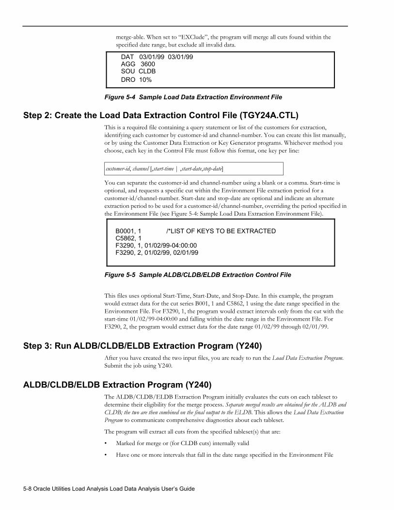
merge-able. When set to “EXClude”, the program will merge all cuts found within the specified date range, but exclude all invalid data.
Figure 5-4 Sample Load Data Extraction Environment File
Step 2: Create the Load Data Extraction Control File (TGY24A.CTL)This is a required file containing a query statement or list of the customers for extraction, identifying each customer by customer-id and channel-number. You can create this list manually, or by using the Customer Data Extraction or Key Generator programs. Whichever method you choose, each key in the Control File must follow this format, one key per line:
You can separate the customer-id and channel-number using a blank or a comma. Start-time is optional, and requests a specific cut within the Environment File extraction period for a customer-id/channel-number. Start-date and stop-date are optional and indicate an alternate extraction period to be used for a customer-id/channel-number, overriding the period specified in the Environment File (see Figure 5-4: Sample Load Data Extraction Environment File).
Figure 5-5 Sample ALDB/CLDB/ELDB Extraction Control File
This files uses optional Start-Time, Start-Date, and Stop-Date. In this example, the program would extract data for the cut series B001, 1 and C5862, 1 using the date range specified in the Environment File. For F3290, 1, the program would extract intervals only from the cut with the start-time 01/02/99-04:00:00 and falling within the date range in the Environment File. For F3290, 2, the program would extract data for the date range 01/02/99 through 02/01/99.
Step 3: Run ALDB/CLDB/ELDB Extraction Program (Y240)After you have created the two input files, you are ready to run the Load Data Extraction Program. Submit the job using Y240.
ALDB/CLDB/ELDB Extraction Program (Y240)The ALDB/CLDB/ELDB Extraction Program initially evaluates the cuts on each tableset to determine their eligibility for the merge process. Separate merged results are obtained for the ALDB and CLDB; the two are then combined on the final output to the ELDB. This allows the Load Data Extraction Program to communicate comprehensive diagnostics about each tableset.
The program will extract all cuts from the specified tableset(s) that are:
• Marked for merge or (for CLDB cuts) internally valid
• Have one or more intervals that fall in the date range specified in the Environment File
DAT 03/01/99 03/01/99AGG 3600SOU CLDBDRO 10%
customer-id, channel [,start-time | ,start-date,stop-date]
B0001, 1 /*LIST OF KEYS TO BE EXTRACTEDC5862, 1F3290, 1, 01/02/99-04:00:00F3290, 2, 01/02/99, 02/01/99
5-8 Oracle Utilities Load Analysis Load Data Analysis User’s Guide

Once the data is extracted, the program merges all cuts for each individual customer-id and channel-number into a new ELDB cut for the extraction period, using the following guidelines:
• Merging is performed in chronological order.
• If the units-of-measure between two cuts are not compatible, the first cut is filled with missing intervals (value zero with status code of 9) up to the start time of the more recent cut. For example, merging two cuts with the same Cust ID but two incompatible UOM's (the first cut was degrees and the second cut was dollars) and start and stop times of 7/1/81 through 8/1/81 (the first cut) and 8/2/81 through 8/30/81 (the second cut) would result in the entire first being replaced with missing intervals. See UOM Compatibility in Appendix J: Oracle Utilities Unit of Measure Codes for more information about compatible UOMs.
• Only data in the extraction period is merged.
• If an overlap occurs, the chronologically most recent data is used.
• If a gap occurs, “0” with a status code of ‘9’ is entered for each missing interval.
• Merged data excludes invalid data, and “0” with a status code of ‘9’ is entered for each excluded interval.
If a cut with the same cut key already exists in the ELDB, the old data will be replaced by the new cut.
Each cut entered into the ELDB will have the following characteristics:
• Start-time is 00:00:00; stop-time is 23:59:59
• Meter information fields are set to zero
• Validation messages are set to blank
• Internal and external validation flags are set to Y (Yes); Edit, Archive, and Merge flags are set to N (No).
Getting Data into the Extracted Load Database (Y130, Y220, Y240) 5-9

5-10 Oracle Utilities Load Analysis Load Data Analysis User’s Guide
Chapter 6Modifying Customer Load Data Prior to Analysis
Using the ELDB Load Data Editor (Y630)
This chapter introduces the ELDB Load Data Editor, which enables you to modify customer load data records in the ELDB. You might use this program to correct bad or missing data, or to create new cuts from old ones.
Topics covered in this chapter:
• Overview
• Using the Load Data Reporter to Examine Cuts
• Steps for Using the ELDB Load Data Editor (Y630)
The kinds of modifications you can make with the Editor are fairly straightforward (e.g., cutting and pasting data and specifying old values for new ones). If you need to combine records or perform calculations on the data, see Chapter 15: Performing Ad Hoc Load Calculations Using the Transformation Program (X620, Y620).
Modifying Customer Load Data Prior to Analysis Using the ELDB Load Data Editor (Y630) 6-1
Overview
OverviewOccasionally, you may need to modify customer load data in the ELDB before applying the analysis programs to it. For example, if you were performing an analysis for forecasting purposes, you would probably replace any outages in a customer’s record with estimated values. (Although the outages reflect actual customer usage, they are likely to be abnormal events that are not appropriate to include in forecasts of future use.) Or, let’s say you wanted to analyze a hypothetical case and needed to synthesize test data from existing cuts. In either case, you could use the Load Data Editor.
The ELDB Load Data Editor enables you to change a cut’s descriptive information and interval data values, and to synthesize new cuts from existing ones. Another important application of the Editor is to delete load data records and other unwanted cuts from the ELDB after you have finished processing them. You can use the ERASE Command to perform this operation.
The kinds of changes that you can make using the ELDB Load Data Editor are primarily “cut and paste” and other direct modifications (in other words, you directly replace an old data value with a new one). Another Oracle Utilities Load Analysis program, Transformation, is available for more complex tasks — such as combining records for multiple channel numbers into a single customer record or calculating new data using arithmetic operations. Transformation is described in Chapter 15: Performing Ad Hoc Load Calculations Using the Transformation Program (X620, Y620).
The ELDB Load Data Editor is identical to the Editor used in the Load Data Management Subsystem, except that the “AUDIT OFF” mode of operation is normally used. This means that edit trails and inactive records of original data are not created during editing, and that the RESTORE Command will not work. All other commands remain the same except PRORATE and REMARK, which are also not available.
6-2 Oracle Utilities Load Analysis Load Data Analysis User’s Guide
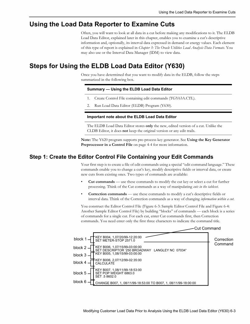
Using the Load Data Reporter to Examine Cuts
Using the Load Data Reporter to Examine CutsOften, you will want to look at all data in a cut before making any modifications to it. The ELDB Load Data Editor, explained later in this chapter, enables you to examine a cut’s descriptive information and, optionally, its interval data expressed in demand or energy values. Each element of this type of report is explained in Chapter 3: The Oracle Utilities Load Analysis Data Formats. You may also use or the Interval Data Manager (IDM) to view data.
Steps for Using the ELDB Load Data Editor (Y630)Once you have determined that you want to modify data in the ELDB, follow the steps summarized in the following box.
Note: The Y620 program supports pre-process key generator. See Using the Key Generator Preprocessor in a Control File on page 4-4 for more information.
Step 1: Create the Editor Control File Containing your Edit CommandsYour first step is to create a file of edit commands using a special “edit command language.” These commands enable you to change a cut’s key, modify descriptive fields or interval data, or create new cuts from existing ones. Two types of commands are available:
• Cut commands — use these commands to modify the cut key or select a cut for further processing. Think of the Cut commands as a way of manipulating cuts in the tableset.
• Correction commands — use these commands to modify a cut’s descriptive fields or interval data. Think of the Correction commands as a way of changing information within a cut.
You construct the Editor Control File (Figure 6-3: Sample Editor Control File and Figure 6-4: Another Sample Editor Control File) by building “blocks” of commands — each block is a series of commands for a single cut. For each cut, enter Cut commands first, then Correction commands. You need enter only the first three characters to indicate the command title.
Summary — Using the ELDB Load Data Editor
1. Create Control File containing edit commands (TGY63A.CTL).
2. Run Load Data Editor (ELDB) Program (Y630).
Important note about the ELDB Load Data Editor
The ELDB Load Data Editor stores only the new, edited version of a cut. Unlike the CLDB Editor, it does not keep the original version or any edit trails.
KEY B004, 1,07/20/99-12:20:00SET METER-STOP 2571.0
KEY B006, 1,07/15/99-03:00:00SET DESCRIPTOR ‘250 BROADWAY LANGLEY NC 07034’KEY B005, 1,08/15/99-03:00:00
KEY B006, 2,07/12/99-02:35:00CALCULATE
KEY B007, 1,08/11/99-18:53:00SET POP WEIGHT 6863.0SET .5 8602.0
CHANGE B007, 1, 08/11/99-18:53:00 TO B007, 1, 08/11/99-18:00:00
block 1
block 2
block 3
block 4
block 5
block 6
Cut Command
CorrectionCommand
Modifying Customer Load Data Prior to Analysis Using the ELDB Load Data Editor (Y630) 6-3
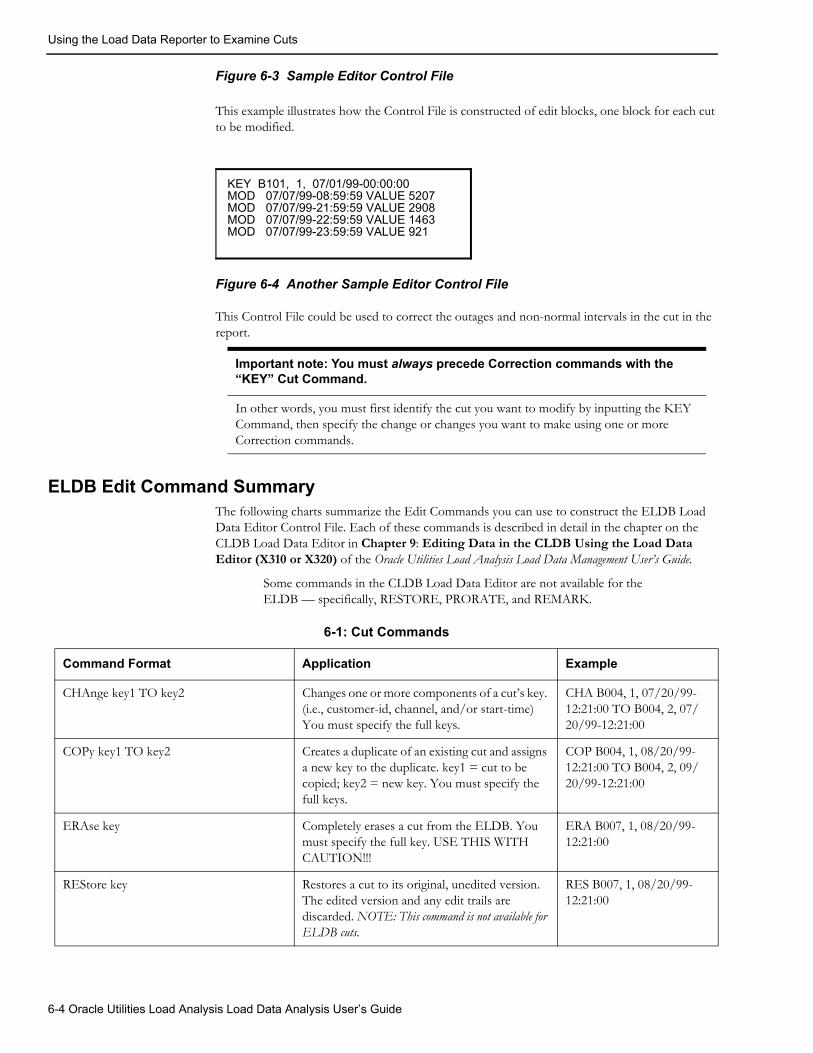
Using the Load Data Reporter to Examine Cuts
Figure 6-3 Sample Editor Control File
This example illustrates how the Control File is constructed of edit blocks, one block for each cut to be modified.
Figure 6-4 Another Sample Editor Control File
This Control File could be used to correct the outages and non-normal intervals in the cut in the report.
ELDB Edit Command SummaryThe following charts summarize the Edit Commands you can use to construct the ELDB Load Data Editor Control File. Each of these commands is described in detail in the chapter on the CLDB Load Data Editor in Chapter 9: Editing Data in the CLDB Using the Load Data Editor (X310 or X320) of the Oracle Utilities Load Analysis Load Data Management User’s Guide.
Some commands in the CLDB Load Data Editor are not available for the ELDB — specifically, RESTORE, PRORATE, and REMARK.
Important note: You must always precede Correction commands with the “KEY” Cut Command.
In other words, you must first identify the cut you want to modify by inputting the KEY Command, then specify the change or changes you want to make using one or more Correction commands.
KEY B101, 1, 07/01/99-00:00:00MOD 07/07/99-08:59:59 VALUE 5207MOD 07/07/99-21:59:59 VALUE 2908MOD 07/07/99-22:59:59 VALUE 1463MOD 07/07/99-23:59:59 VALUE 921
6-1: Cut Commands
Command Format Application Example
CHAnge key1 TO key2 Changes one or more components of a cut’s key. (i.e., customer-id, channel, and/or start-time) You must specify the full keys.
CHA B004, 1, 07/20/99-12:21:00 TO B004, 2, 07/20/99-12:21:00
COPy key1 TO key2 Creates a duplicate of an existing cut and assigns a new key to the duplicate. key1 = cut to be copied; key2 = new key. You must specify the full keys.
COP B004, 1, 08/20/99-12:21:00 TO B004, 2, 09/20/99-12:21:00
ERAse key Completely erases a cut from the ELDB. You must specify the full key. USE THIS WITH CAUTION!!!
ERA B007, 1, 08/20/99-12:21:00
REStore key Restores a cut to its original, unedited version.The edited version and any edit trails are discarded. NOTE: This command is not available for ELDB cuts.
RES B007, 1, 08/20/99-12:21:00
6-4 Oracle Utilities Load Analysis Load Data Analysis User’s Guide
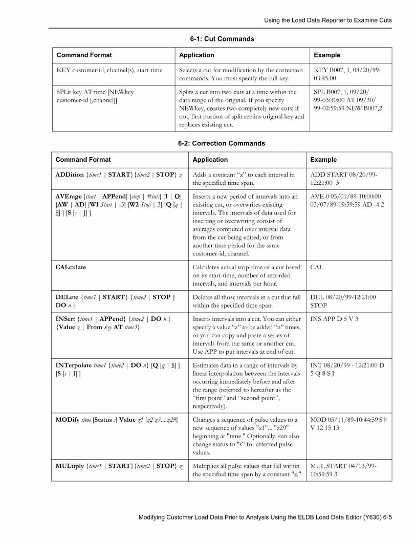
Using the Load Data Reporter to Examine Cuts
KEY customer-id, channel(s), start-time Selects a cut for modification by the correction commands. You must specify the full key.
KEY B007, 1, 08/20/99-03:45:00
SPLit key AT time [NEWkey customer-id [,channel]]
Splits a cut into two cuts at a time within the data range of the original. If you specify NEWkey, creates two completely new cuts; if not, first portion of split retains original key and replaces existing cut.
SPL B007, 1, 09/20/99-03:30:00 AT 09/30/99-02:59:59 NEW B007,2
6-1: Cut Commands
Command Format Application Example
6-2: Correction Commands
Command Format Application Example
ADDition {time1 | START}{time2 | STOP} z Adds a constant “z” to each interval in the specified time span.
ADD START 08/20/99-12:21:00 3
AVErage [start | APPend] [stop | #ints] [I | O] [AW | AD] [W1 Start | -3] [W2 Stop | 3] [Q [q | 8] ] [S [s | J] ]
Inserts a new period of intervals into an existing cut, or overwrites existing intervals. The intervals of data used for inserting or overwriting consist of averages computed over interval data from the cut being edited, or from another time period for the same customer-id, channel.
AVE 0 03/01/89-10:00:0003/07/89-09:59:59 AD -4 2
CALculate Calculates actual stop-time of a cut based on its start-time, number of recorded intervals, and intervals per hour.
CAL
DELete {time1 | START} {time2 | STOP | DO n }
Deletes all those intervals in a cut that fall within the specified time span.
DEL 08/20/99-12:21:00 STOP
INSert {time1 | APPend} {time2 | DO n } {Value z | From key AT time3}
Inserts intervals into a cut. You can either specify a value “z” to be added “n” times, or you can copy and paste a series of intervals from the same or another cut. Use APP to put intervals at end of cut.
INS APP D 5 V 3
INTerpolate time1 {time2 | DO n} [Q [q | 8] ] [S [s | J] ]
Estimates data in a range of intervals by linear interpolation between the intervals occurring immediately before and after the range (referred to hereafter as the “first point” and “second point”, respectively).
INT 08/20/99 - 12:21:00 D 5 Q 8 S J
MODify time [Status s] Value z1 [z2 z3... z29] Changes a sequence of pulse values to a new sequence of values "z1"... "z29" beginning at "time." Optionally, can also change status to "s" for affected pulse values.
MOD 05/11/89-10:44:59 S 9 V 12 15 13
MULtiply {time1 | START}{time2 | STOP} z Multiplies all pulse values that fall within the specified time span by a constant "z."
MUL START 04/13/99-10:59:59 3
Modifying Customer Load Data Prior to Analysis Using the ELDB Load Data Editor (Y630) 6-5
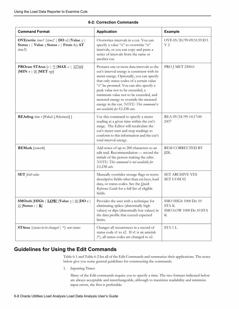
Using the Load Data Reporter to Examine Cuts
Guidelines for Using the Edit CommandsTable 6-1 and Table 6-2 list all of the Edit Commands and summarize their applications. The notes below give you some general guidelines for constructing the commands.
1. Inputting Times
Many of the Edit commands require you to specify a time. The two formats indicated below are always acceptable and interchangeable, although to maximize readability and minimize input errors, the first is preferable:
OVErwrite time1 {time2 | DO n}{Value z | Status s | Value z Status s | From key AT time3}
Overwrites intervals in a cut. You can specify a value “z” to overwrite “n” intervals, or you can copy and paste a series of intervals from the same or another cut.
OVE 05/20/99-09:51:59 D 5 V 2
PROrate STAtus [s | *] [MAX x | 32760] [MIN n | 0] [MET ngy]
Prorates one or more data intervals so the cut’s interval energy is consistent with its meter energy. Optionally, you can specify that only status codes of a certain value “s” be prorated. You can also specify a peak value not to be exceeded, a minimum value not to be exceeded, and metered energy to override the metered energy in the cut. NOTE: This command is not available for ELDB cuts.
PRO J MET 2500.0
REAding time r [#dials [.#decimals] ] Use this command to specify a meter reading at a given time within the cut’s range. The Editor will recalculate the cut’s meter start and stop readings to conform to this information and the cut’s total interval energy.
REA 09/24/99-14:17:00 2437
REMark [remark] Add notes of up to 200 characters to an edit trail. Recommendation — record the initials of the person making the edits. NOTE: This command is not available for ELDB cuts.
REM CORRECTED BY JDL
SET field value Manually overrides storage flags or resets descriptive fields other than cut keys, load data, or status codes. See the Quick Reference Guide for a full list of eligible fields.
SET ARCHIVE YESSET UOM 02
SMOoth [HIGh | LOW] [Value z | 0] [DO n | 1] [Status s | K]
Provides the user with a technique for eliminating spikes (abnormally high values) or dips (abnormally low values) in the data profile that exceed expected limits.
SMO HIGh 1000 Do 10 STA KSMO LOW 1000 Do 10 STA K
STAtus {status-to-be-changed | *} new-status Changes all occurrences in a record of status code s1 to s2. If s1 is an asterisk (*), all status codes are changed to s2.
STA 1 L
6-2: Correction Commands
Command Format Application Example
6-6 Oracle Utilities Load Analysis Load Data Analysis User’s Guide
Using the Load Data Reporter to Examine Cuts
• mm/dd/yy-hh:mm:ss (for example, 01/23/89-00:00:00)
• mmddyyhhmmss (for example, 012389000000).
In the KEY Command, it is permissible to use just the start-date.
2. Specifying Interval Values for Modification
Many of the Correction commands enable you to change one or a series of interval values in a cut. You must identify which values you want to change by specifying parameters in the command. You can do this in a couple of ways:
• “Time1" “Time2" — You can identify the ending time of the first and last intervals in the series to be changed, e.g., “time1 time2”. You must input the complete date and time.
• “START” “STOP” — If the first interval in the group you want to change is the first interval in the cut, you can input “START” instead of typing out the time. Similarly, if the last interval in the group you want to change is the last interval in the cut, you can input “STOP”.
• “DO n” — You can indicate the first interval in the series (using either its ending time or START) and the number of intervals after it if you want them changed using “DO n”, where n = the number of intervals to be changed. You can enter “D” for DO.
• “Value z” — Identify the value to be added, etc., to each specified interval by “Value = z”, where z is the constant. You can abbreviate Value by just using the letter “V”.
3. Patching Interval Data
The INSERT, INTERPOLATE, and OVERWRITE commands enable you to copy, paste, and estimate interval data from one cut to another. You can copy a series of energy values from the same cut or any other cut in the ELDB. The intervals can even be from two contiguous cuts. If the cut being copied has a different pulse multiplier than the cut being edited, the data values will be adjusted using the edited cut’s multiplier before the values are copied. You use “From key AT time” and “DO n” to specify the intervals to be copied, where “key” is the key of the source cut, “time” is the ending time of the first interval to be copied, and n is the number of intervals to be copied. AVERAGE also does patching, but only within a cut series.
Step 2: Run the ELDB Load Data Editor Procedure (Y630)Once you have created the Control File, you are ready to run the ELDB Load Data Editor. Use the Y630 Submit screen.
For a more detailed explanation of the Load Data Editor, please refer to the Oracle Utilities Load Analysis Load Data Management User’s Guide, Chapter 9.
Modifying Customer Load Data Prior to Analysis Using the ELDB Load Data Editor (Y630) 6-7

Using the Load Data Reporter to Examine Cuts
6-8 Oracle Utilities Load Analysis Load Data Analysis User’s Guide
Chapter 7Expanding Load Data to Class-Level Estimates
Using the Load Analysis Programs (Y310 andY330)
Once you have input data to the Extracted Load Database and (possibly) modified it to your requirements, you are ready to begin analysis. Oracle Utilities Load Analysis offers two programs for developing strata- and class-level statistics from customer load data: Standard Load Analysis and Ratio Analysis. This chapter explains how to apply each program. Topics covered are:
• Comparison of MPU and Ratio Analysis Methodologies
• Three Methods of Ratio Estimating
• Preparing for Analysis
• Steps for Using the Standard Load Analysis or Ratio Analysis Procedures (Y310 or Y330)
Oracle Utilities Load Analysis offers a third program for computing statistics for a single analysis group — the 100% Sample Analysis Program. That program, which is described in the following chapter, is used when every member of the population is included in the analysis.
Expanding Load Data to Class-Level Estimates Using the Load Analysis Programs (Y310 and Y330) 7-1
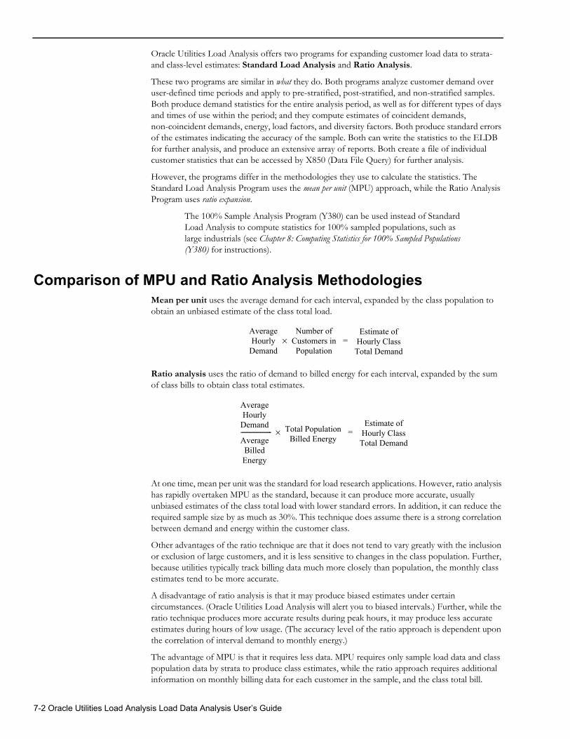
Oracle Utilities Load Analysis offers two programs for expanding customer load data to strata- and class-level estimates: Standard Load Analysis and Ratio Analysis.
These two programs are similar in what they do. Both programs analyze customer demand over user-defined time periods and apply to pre-stratified, post-stratified, and non-stratified samples. Both produce demand statistics for the entire analysis period, as well as for different types of days and times of use within the period; and they compute estimates of coincident demands, non-coincident demands, energy, load factors, and diversity factors. Both produce standard errors of the estimates indicating the accuracy of the sample. Both can write the statistics to the ELDB for further analysis, and produce an extensive array of reports. Both create a file of individual customer statistics that can be accessed by X850 (Data File Query) for further analysis.
However, the programs differ in the methodologies they use to calculate the statistics. The Standard Load Analysis Program uses the mean per unit (MPU) approach, while the Ratio Analysis Program uses ratio expansion.
The 100% Sample Analysis Program (Y380) can be used instead of Standard Load Analysis to compute statistics for 100% sampled populations, such as large industrials (see Chapter 8: Computing Statistics for 100% Sampled Populations (Y380) for instructions).
Comparison of MPU and Ratio Analysis MethodologiesMean per unit uses the average demand for each interval, expanded by the class population to obtain an unbiased estimate of the class total load.
Ratio analysis uses the ratio of demand to billed energy for each interval, expanded by the sum of class bills to obtain class total estimates.
At one time, mean per unit was the standard for load research applications. However, ratio analysis has rapidly overtaken MPU as the standard, because it can produce more accurate, usually unbiased estimates of the class total load with lower standard errors. In addition, it can reduce the required sample size by as much as 30%. This technique does assume there is a strong correlation between demand and energy within the customer class.
Other advantages of the ratio technique are that it does not tend to vary greatly with the inclusion or exclusion of large customers, and it is less sensitive to changes in the class population. Further, because utilities typically track billing data much more closely than population, the monthly class estimates tend to be more accurate.
A disadvantage of ratio analysis is that it may produce biased estimates under certain circumstances. (Oracle Utilities Load Analysis will alert you to biased intervals.) Further, while the ratio technique produces more accurate results during peak hours, it may produce less accurate estimates during hours of low usage. (The accuracy level of the ratio approach is dependent upon the correlation of interval demand to monthly energy.)
The advantage of MPU is that it requires less data. MPU requires only sample load data and class population data by strata to produce class estimates, while the ratio approach requires additional information on monthly billing data for each customer in the sample, and the class total bill.
AverageHourly
Demand
Number ofCustomers inPopulation
×Estimate of
Hourly ClassTotal Demand
=
AverageHourly
Demand
AverageBilledEnergy
---------------------- Total PopulationBilled Energy
×Estimate of
Hourly ClassTotal Demand
=
7-2 Oracle Utilities Load Analysis Load Data Analysis User’s Guide
Three Methods of Ratio EstimatingThe Ratio Analysis Program can perform three types of ratio estimation. Each technique has its own formulation and statistical assumptions for correct usage. Which technique the program applies is automatically dictated by commands you supply in the Environment File.
Non-Stratified Ratio — applies only to simple random samples with no stratification. The program automatically uses this technique when you supply a single STRATA Command in the Environment File.
Stratified Combined Ratio — most commonly used estimator for stratified random samples. It calculates a “combined ratio” across all strata and expands it by the total population billed energy. This technique produces demand estimates for the class; it does not produce stratum-level demand estimates.
Stratified Separate Ratio — effective methodology if the relationship of demand to energy changes significantly from one stratum to the next. It requires that you supply accurate billed energy totals for each stratum. It produces demand estimates for each stratum, and the class total.
Preparing for AnalysisBefore running the Analysis programs, you will construct a “Control File” consisting of a list of customers and related data to be analyzed, and an “Environment File” specifying the analysis mode and various reporting options. Here are some useful guidelines to keep in mind when getting ready to construct these files. Each piece of information is described in more detail later in this chapter.
1. Customer Data
For each customer included in the analysis, you will need to identify its stratum-number (if using stratified analysis) and its billed energy for the billing cycle(s) that correspond to the analysis period (if using any of the three types of Ratio Analysis). The stratum-number will typically come from the original sample design. The billed energy may come from “the Billing System.” For example, your facility may have an interface software program that extracts the data from Billing or a Customer Master File. The customer billed energy values for a Ratio Analysis should be reviewed carefully to ensure that they are complete and correspond to the billing period covered by the analysis.
If you cannot supply billed energy values for individual customers, the Ratio Analysis Program can calculate the energy values for the analysis period using the customers’ interval data as part of the analysis job run. A better alternative, however, is to use the Billed Energy Program, Y230 (described in Chapter 13: Computing Customer Energy Use by Billing Cycles Using the Billed Energy Program (Y230)) to calculate energy for the appropriate billing periods. (This is explained further in Step 2 of this chapter.)
2. Load Data
You can analyze any customer subset and any time period for which data exists in the ELDB.
3. Population
Strata Sizes — If performing stratified analysis, you will need to specify the size of each stratum's population for that bill cycle or the population of that stratum from the original sample design. The population of the current stratum is desirable. This number is calculated by taking each premises energy or billed energy and fitting it into the strata boundaries, then counting that premise into the population of that strata.
Population Billed Energy — If applying ratio analysis, you will need to input the actual value of the billed energy for the sample over the analysis period. If you know the actual billed energy for each stratum, you can perform Separate Ratio Estimation. However, if you do not have the billed energy for the sample accurately broken down by strata, you will have to use Combined Ratio Estimation.
Expanding Load Data to Class-Level Estimates Using the Load Analysis Programs (Y310 and Y330) 7-3
Sample Points — It is important to remember that each entry in the Control File is a sample point. If you are analyzing end uses, it would be appropriate to keep channel-numbers separate. If you are analyzing “total premise loads,” you may want to combine the channel-numbers for a single customer. You can do that in the Analysis Control File or in the Y620 - Transformation or Totalizing reporter programs. (You can create a Sequencer to accomplish both the totalization and analysis runs.) However, if you want to combine multiple customer-ids for a large individual customer to create a single sample point, you will have to use the Load Data Transformation Program, Y620, before analysis (described in Chapter 15: Performing Ad Hoc Load Calculations Using the Transformation Program (X620, Y620)).
4. Saving Results
In the Analysis Environment File, Oracle Utilities Load Analysis will ask you to assign a key identifier to the analysis results. It is very important — particularly if the statistics are to be accessed by people besides yourself — that you assign a meaningful key. For example, you might assign the key “RESAC” to the results of a residential air conditioning study. You may also direct the program to write statistics back to an ELDB designated for a specific rate code or directly into an SLDB.
7-4 Oracle Utilities Load Analysis Load Data Analysis User’s Guide
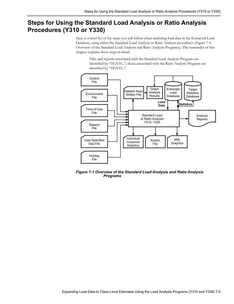
Steps for Using the Standard Load Analysis or Ratio Analysis Procedures (Y310 or Y330)
Steps for Using the Standard Load Analysis or Ratio Analysis Procedures (Y310 or Y330)
Here is a brief list of the steps you will follow when analyzing load data in the Extracted Load Database, using either the Standard Load Analysis or Ratio Analysis procedures (Figure 7-1: Overview of the Standard Load Analysis and Ratio Analysis Programs). The remainder of this chapter explains these steps in detail.
Files and reports associated with the Standard Load Analysis Program are identified by “TGY31_”; those associated with the Ratio Analysis Program are identified by “TGY33_”.
Figure 7-1 Overview of the Standard Load Analysis and Ratio Analysis Programs
ExtractedLoad
Database
StatisticsLoadData
SeasonFile
User-Specified Day File
Standard Loador Ratio Analysis
Y310, Y330
AnalysisReports
IndividualCustomerStatistics
KeylistFile
ControlFile
HolidayFile
EnvironmentFile
Time-of-UseFile
TargetStatisticsDatabase
GraphAnalysisResults
XMLGraphics
Statistic KeysWritten File
Expanding Load Data to Class-Level Estimates Using the Load Analysis Programs (Y310 and Y330) 7-5
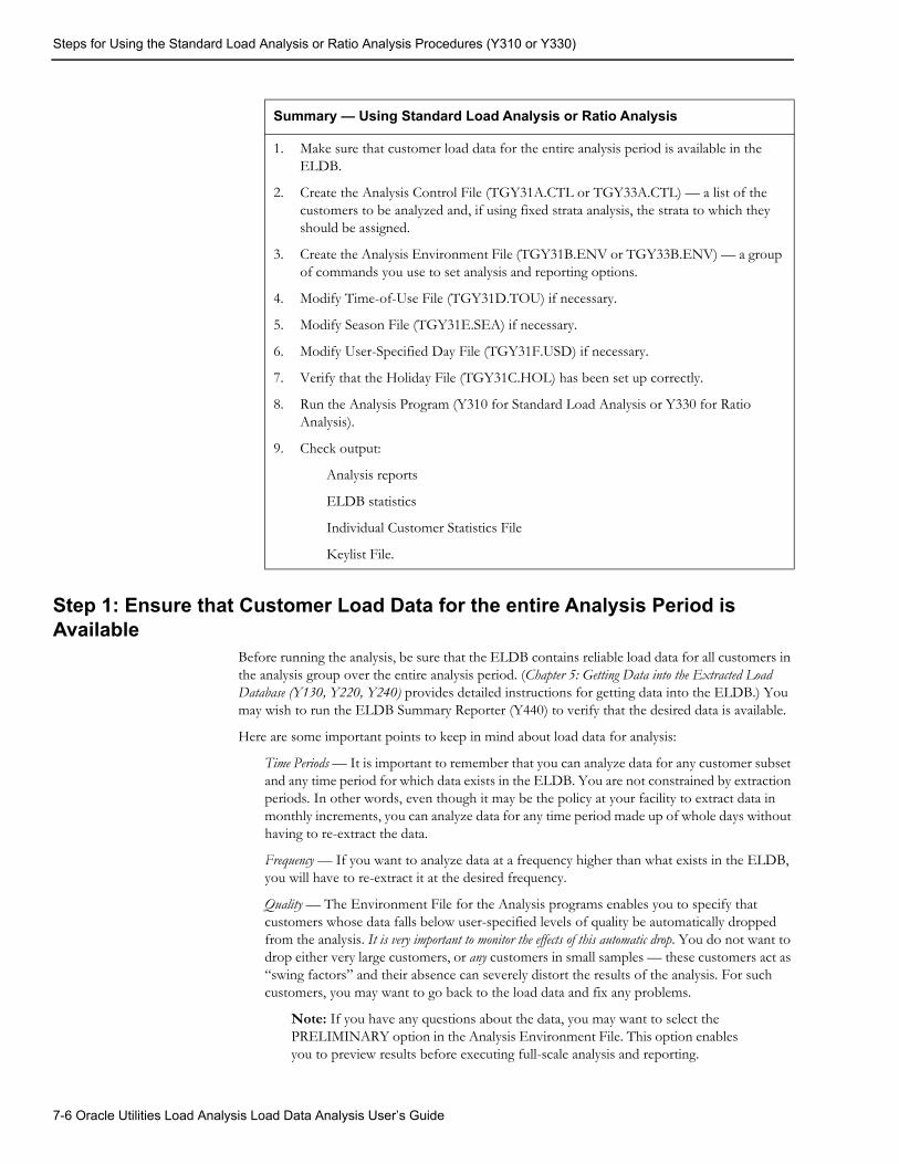
Steps for Using the Standard Load Analysis or Ratio Analysis Procedures (Y310 or Y330)
Step 1: Ensure that Customer Load Data for the entire Analysis Period is Available
Before running the analysis, be sure that the ELDB contains reliable load data for all customers in the analysis group over the entire analysis period. (Chapter 5: Getting Data into the Extracted Load Database (Y130, Y220, Y240) provides detailed instructions for getting data into the ELDB.) You may wish to run the ELDB Summary Reporter (Y440) to verify that the desired data is available.
Here are some important points to keep in mind about load data for analysis:
Time Periods — It is important to remember that you can analyze data for any customer subset and any time period for which data exists in the ELDB. You are not constrained by extraction periods. In other words, even though it may be the policy at your facility to extract data in monthly increments, you can analyze data for any time period made up of whole days without having to re-extract the data.
Frequency — If you want to analyze data at a frequency higher than what exists in the ELDB, you will have to re-extract it at the desired frequency.
Quality — The Environment File for the Analysis programs enables you to specify that customers whose data falls below user-specified levels of quality be automatically dropped from the analysis. It is very important to monitor the effects of this automatic drop. You do not want to drop either very large customers, or any customers in small samples — these customers act as “swing factors” and their absence can severely distort the results of the analysis. For such customers, you may want to go back to the load data and fix any problems.
Note: If you have any questions about the data, you may want to select the PRELIMINARY option in the Analysis Environment File. This option enables you to preview results before executing full-scale analysis and reporting.
Summary — Using Standard Load Analysis or Ratio Analysis
1. Make sure that customer load data for the entire analysis period is available in the ELDB.
2. Create the Analysis Control File (TGY31A.CTL or TGY33A.CTL) — a list of the customers to be analyzed and, if using fixed strata analysis, the strata to which they should be assigned.
3. Create the Analysis Environment File (TGY31B.ENV or TGY33B.ENV) — a group of commands you use to set analysis and reporting options.
4. Modify Time-of-Use File (TGY31D.TOU) if necessary.
5. Modify Season File (TGY31E.SEA) if necessary.
6. Modify User-Specified Day File (TGY31F.USD) if necessary.
7. Verify that the Holiday File (TGY31C.HOL) has been set up correctly.
8. Run the Analysis Program (Y310 for Standard Load Analysis or Y330 for Ratio Analysis).
9. Check output:
Analysis reports
ELDB statistics
Individual Customer Statistics File
Keylist File.
7-6 Oracle Utilities Load Analysis Load Data Analysis User’s Guide
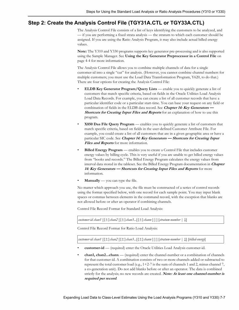
Steps for Using the Standard Load Analysis or Ratio Analysis Procedures (Y310 or Y330)
Step 2: Create the Analysis Control File (TGY31A.CTL or TGY33A.CTL)The Analysis Control File consists of a list of keys identifying the customers to be analyzed, and — if you are performing a fixed strata analysis — the stratum to which each customer should be assigned. If you are using the Ratio Analysis Program, it may also include actual billed energy values.
Note: The Y310 and Y330 programs supports key generator pre-processing and is also supported using the Sample Manager. See Using the Key Generator Preprocessor in a Control File on page 4-4 for more information.
The Analysis Control File allows you to combine multiple channels of data for a single customer-id into a single “cut” for analysis. (However, you cannot combine channel numbers for multiple customers; you must use the Load Data Transformation Program, Y620, to do that.) There are four options for creating the Analysis Control File:
• ELDB Key Generator Program/Query Lists — enable you to quickly generate a list of customers that match specific criteria, based on fields in the Oracle Utilities Load Analysis Load Data Records. For example, you can create a list of all customer records that have a particular identifier code or a particular start-time. You can base your request on any field or combination of fields in the ELDB data record. See Chapter 14: Key Generators — Shortcuts for Creating Input Files and Reports for an explanation of how to use this program.
• X850 Daa File Query Program — enables you to quickly generate a list of customers that match specific criteria, based on fields in the user-defined Customer Attribute File. For example, you could create a list of all customers that are in a given geographic area or have a particular SIC code. See Chapter 14: Key Generators — Shortcuts for Creating Input Files and Reports for more information.
• Billed Energy Program — enables you to create a Control File that includes customer energy values by billing cycle. This is very useful if you are unable to get billed energy values from “books and records.” The Billed Energy Program calculates the energy values from interval data stored in the tableset. See the Billed Energy Program documentation in Chapter 14: Key Generators — Shortcuts for Creating Input Files and Reports for more information.
• Manually — you can type the file.
No matter which approach you use, the file must be constructed of a series of control records using the format specified below, with one record for each sample point. You may input blank spaces or commas between elements in the command record, with the exception that blanks are not allowed before or after an operator if combining channels.
Control File Record Format for Standard Load Analysis:
Control File Record Format for Ratio Load Analysis:
• customer-id — (required) enter the Oracle Utilities Load Analysis customer-id.
• chan1, chan2...chanx — (required) enter the channel-number or a combination of channels for that customer-id. A combination consists of two or more channels added or subtracted to represent the total customer load (e.g., 1+2-7 is the sum of channels 1 and 2, minus channel 7, a co-generation unit). Do not add blanks before or after an operator. The data is combined strictly for the analysis; no new records are created. Note: At least one channel-number is required per record.
customer-id chan1 [{±}chan2 [{±}chan3...[{±}chann ] ] ] [stratum-number | 1]
customer-id chan1 [{±}chan2 [{±}chan3...[{±}chann ] ] ] [stratum-number | 1] [billed-energy]
Expanding Load Data to Class-Level Estimates Using the Load Analysis Programs (Y310 and Y330) 7-7
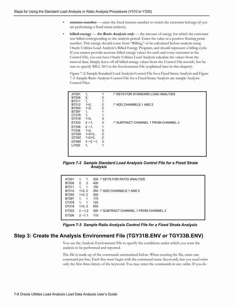
Steps for Using the Standard Load Analysis or Ratio Analysis Procedures (Y310 or Y330)
• stratum-number — enter the fixed stratum number to which the customer belongs (if you are performing a fixed strata analysis).
• billed-energy — for Ratio Analysis only — the amount of energy for which the customer was billed corresponding to the analysis period. Enter the value as a positive floating point number. This energy should come from “Billing,” or be calculated before analysis using Oracle Utilities Load Analysis’s Billed Energy Program, and should represent a billing cycle. If you cannot provide accurate billed energy values for each and every customer in the Control File, you can have Oracle Utilities Load Analysis calculate the values from the interval data. Simply leave off all billed-energy values from the Control File records, but be sure to specify BILL NO in the Environment File (explained later in this chapter).
Figure 7-2: Sample Standard Load Analysis Control File for a Fixed Strata Analysis and Figure 7-3: Sample Ratio Analysis Control File for a Fixed Strata Analysis are sample Analysis Control Files.
Figure 7-2 Sample Standard Load Analysis Control File for a Fixed Strata Analysis
Figure 7-3 Sample Ratio Analysis Control File for a Fixed Strata Analysis
Step 3: Create the Analysis Environment File (TGY31B.ENV or TGY33B.ENV)You use the Analysis Environment File to specify the conditions under which you want the analysis to be performed and reported.
The file is made up of the commands summarized below. When creating the file, enter one command per line. Each line must begin with the command name (keyword); but you need enter only the first three letters of the keyword. You may enter the commands in any order. If you do
A7301 1, 1 /* KEYS FOR STANDARD LOAD ANALYSISB7308 2, 2B7311 1, 1B7312 1+2, 2 /* ADD CHANNELS 1 AND 2B7393 1+2, 2B7397 1, 1C7378 1, 1D7316 1+2, 3E7333 2 –1, 2 /* SUBTRACT CHANNEL 1 FROM CHANNEL 2E7336 2 –1, 1F7338 1+2, 3G7339 1+2+3, 2G7342 1+2+3, 2G7480 3 –2 –1, 3L7353 1, 1
A7301 1, 1 200 /* KEYS FOR RATIO ANALYSISB7308 2, 2 400B7311 1, 1 150B7312 1+2, 2 350 /* ADD CHANNELS 1 AND 2B7393 1+2, 2 300B7397 1, 1 175C7378 1, 1 125D7316 1+2, 3 650E7333 2 –1,2 300 /* SUBTRACT CHANNEL 1 FROM CHANNEL 2E7336 2 –1,1 110
7-8 Oracle Utilities Load Analysis Load Data Analysis User’s Guide
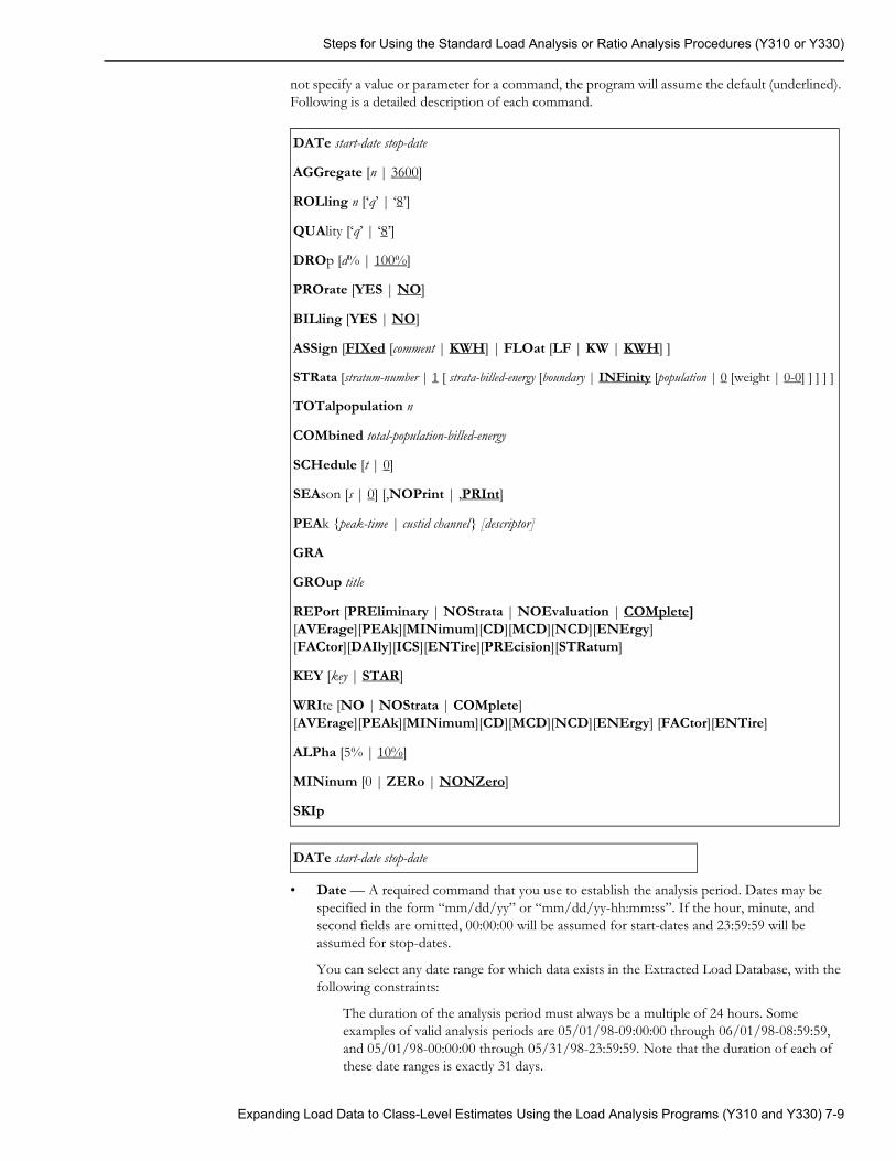
Steps for Using the Standard Load Analysis or Ratio Analysis Procedures (Y310 or Y330)
not specify a value or parameter for a command, the program will assume the default (underlined). Following is a detailed description of each command.
• Date — A required command that you use to establish the analysis period. Dates may be specified in the form “mm/dd/yy” or “mm/dd/yy-hh:mm:ss”. If the hour, minute, and second fields are omitted, 00:00:00 will be assumed for start-dates and 23:59:59 will be assumed for stop-dates.
You can select any date range for which data exists in the Extracted Load Database, with the following constraints:
The duration of the analysis period must always be a multiple of 24 hours. Some examples of valid analysis periods are 05/01/98-09:00:00 through 06/01/98-08:59:59, and 05/01/98-00:00:00 through 05/31/98-23:59:59. Note that the duration of each of these date ranges is exactly 31 days.
DATe start-date stop-date
AGGregate [n | 3600]
ROLling n [‘q’ | ‘8’]
QUAlity [‘q’ | ‘8’]
DROp [d% | 100%]
PROrate [YES | NO]
BILling [YES | NO]
ASSign [FIXed [comment | KWH] | FLOat [LF | KW | KWH] ]
STRata [stratum-number | 1 [ strata-billed-energy [boundary | INFinity [population | 0 [weight | 0-0] ] ] ] ]
TOTalpopulation n
COMbined total-population-billed-energy
SCHedule [t | 0]
SEAson [s | 0] [,NOPrint | ,PRInt]
PEAk {peak-time | custid channel} [descriptor]
GRA
GROup title
REPort [PREliminary | NOStrata | NOEvaluation | COMplete] [AVErage][PEAk][MINimum][CD][MCD][NCD][ENErgy] [FACtor][DAIly][ICS][ENTire][PREcision][STRatum]
KEY [key | STAR]
WRIte [NO | NOStrata | COMplete][AVErage][PEAk][MINimum][CD][MCD][NCD][ENErgy] [FACtor][ENTire]
ALPha [5% | 10%]
MINinum [0 | ZERo | NONZero]
SKIp
DATe start-date stop-date
Expanding Load Data to Class-Level Estimates Using the Load Analysis Programs (Y310 and Y330) 7-9
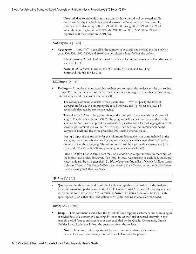
Steps for Using the Standard Load Analysis or Ratio Analysis Procedures (Y310 or Y330)
Note: All data found within any particular 24-hour period will be treated as if it occurs on the day in which that period starts - the “sendout day”. For example, if the specified date range is 05/01/98-09:00:00 through 05/31/98-08:59:59, all intervals occurring between 05/01/98-09:00:00 and 05/02/98-08:59:59 will be reported as if they occur on 05/01/98.
• Aggregate — Input “n” to establish the number of seconds-per-interval for the analysis data; 300, 900, 1800, 3600, and 86400 are permitted values. 3600 is the default.
Where possible, Oracle Utilities Load Analysis will sum each customer’s load data to the specified level.
Note: If AGG 86400 is coded, the SCHedule, SEAson, and ROLling commands should not be used.
• Rolling — An optional command that enables you to report the analysis results in a rolling format. That is, each interval of the analysis period is an average of a number of preceding interval values and the current interval itself.
The rolling command consists of two parameters — “n” to specify the level of aggregation for use in computing the rolled interval, and “q” to set the level of acceptable data quality for the averaging.
The value for “n” must be greater than, and a multiple of, the analysis data’s interval length. The default value is “3600”. The program will average the analysis data at the level set by “n”. For example, if the original analysis data has a level of aggregation of 900 seconds-per-interval and you set “n” to 3600, then each output interval will be the average of itself and the three preceding 900-second interval values.
For “q”, input the status code for the minimum data quality you want included in the averaging. Any intervals that are missing or have status codes worse than “q” will be excluded from the averaging. The status code must be input with apostrophes (’) on either side. The default is ‘8’ (only missing intervals are excluded).
Oracle Utilities Load Analysis sets the status code of an output interval to the worst of the input status codes. However, if an input interval was missing or excluded, the output status code can be no better than ‘5’. Note: You can find a list of Oracle Utilities status codes in Chapter 3: The Oracle Utilities Load Analysis Data Formats, or in the Oracle Utilities Load Analysis Quick Reference Guide.
• Quality — Use this command to set the level of acceptable data quality for the analysis. Input the worst acceptable status code. Oracle Utilities Load Analysis will treat any interval with a status code worse than “q” as missing. Note: The status code must be input with apostrophes (’) on either side. The default is ‘8’ (only missing intervals are excluded).
• Drop — This command establishes the threshold for dropping customers due to missing or excluded data. If a customer is missing d% or more of the total expected intervals in the analysis period (due to missing data or data excluded by the Quality Command), Oracle Utilities Load Analysis will drop the customer from the analysis.
Note: This command is superseded by the requirement that each customer have at least one non-missing interval in each Time-of-Use period.
AGGregate [n | 3600]
ROLling n [‘q’ | ‘8’]
QUAlity [‘q’ | ‘8’]
DROp [d% | 100%]
7-10 Oracle Utilities Load Analysis Load Data Analysis User’s Guide
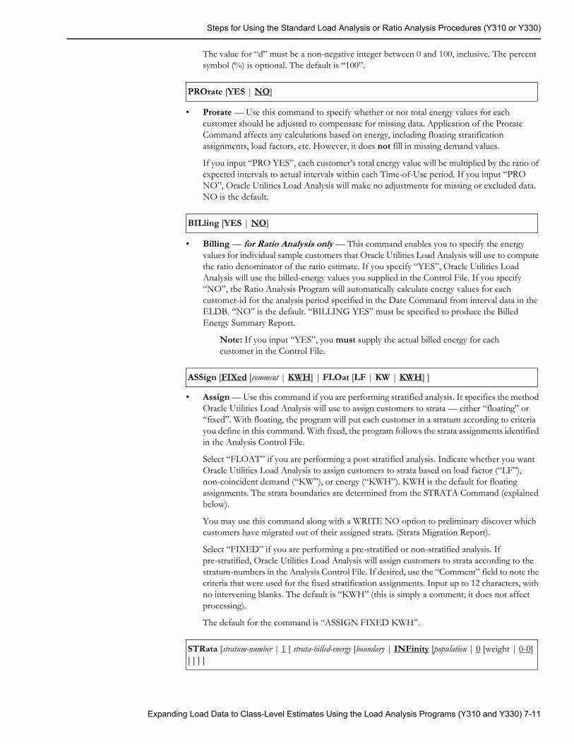
Steps for Using the Standard Load Analysis or Ratio Analysis Procedures (Y310 or Y330)
The value for “d” must be a non-negative integer between 0 and 100, inclusive. The percent symbol (%) is optional. The default is “100”.
• Prorate — Use this command to specify whether or not total energy values for each customer should be adjusted to compensate for missing data. Application of the Prorate Command affects any calculations based on energy, including floating stratification assignments, load factors, etc. However, it does not fill in missing demand values.
If you input “PRO YES”, each customer’s total energy value will be multiplied by the ratio of expected intervals to actual intervals within each Time-of-Use period. If you input “PRO NO”, Oracle Utilities Load Analysis will make no adjustments for missing or excluded data. NO is the default.
• Billing — for Ratio Analysis only — This command enables you to specify the energy values for individual sample customers that Oracle Utilities Load Analysis will use to compute the ratio denominator of the ratio estimate. If you specify “YES”, Oracle Utilities Load Analysis will use the billed-energy values you supplied in the Control File. If you specify “NO”, the Ratio Analysis Program will automatically calculate energy values for each customer-id for the analysis period specified in the Date Command from interval data in the ELDB. “NO” is the default. “BILLING YES” must be specified to produce the Billed Energy Summary Report.
Note: If you input “YES”, you must supply the actual billed energy for each customer in the Control File.
• Assign — Use this command if you are performing stratified analysis. It specifies the method Oracle Utilities Load Analysis will use to assign customers to strata — either “floating” or “fixed”. With floating, the program will put each customer in a stratum according to criteria you define in this command. With fixed, the program follows the strata assignments identified in the Analysis Control File.
Select “FLOAT” if you are performing a post-stratified analysis. Indicate whether you want Oracle Utilities Load Analysis to assign customers to strata based on load factor (“LF”), non-coincident demand (“KW”), or energy (“KWH”). KWH is the default for floating assignments. The strata boundaries are determined from the STRATA Command (explained below).
You may use this command along with a WRITE NO option to preliminary discover which customers have migrated out of their assigned strata. (Strata Migration Report).
Select “FIXED” if you are performing a pre-stratified or non-stratified analysis. If pre-stratified, Oracle Utilities Load Analysis will assign customers to strata according to the stratum-numbers in the Analysis Control File. If desired, use the “Comment” field to note the criteria that were used for the fixed stratification assignments. Input up to 12 characters, with no intervening blanks. The default is “KWH” (this is simply a comment; it does not affect processing).
The default for the command is “ASSIGN FIXED KWH”.
PROrate [YES | NO]
BILling [YES | NO]
ASSign [FIXed [comment | KWH] | FLOat [LF | KW | KWH] ]
STRata [stratum-number | 1 [ strata-billed-energy [boundary | INFinity [population | 0 [weight | 0-0] ] ] ] ]
Expanding Load Data to Class-Level Estimates Using the Load Analysis Programs (Y310 and Y330) 7-11
Steps for Using the Standard Load Analysis or Ratio Analysis Procedures (Y310 or Y330)
• Strata — How you set up the Strata Command(s) largely determines what kind of analysis the program performs. Generally, you will supply one Strata Command for each stratum in a stratified analysis. If you supply just one Strata Command in the file, the program will perform a non-stratified analysis. If you leave out the command altogether, the program will perform the default: non-stratified analysis of a 100% sampled population.
Parameters you supply within the command further influence the type of analysis, as explained below and illustrated later in this section (see Figure 7-4: Sample Environment File for a Stratified Standard Load Analysis through Figure 7-8: Sample Ratio Analysis Environment File for a Non-Stratified Analysis).
Input one command (line) for each stratum in the analysis. Up to 99 strata may be defined. The following explains each parameter in the command:
stratum-number — Identifies the stratum. It must be a positive integer from 1 to 99. Within the file, stratum numbers must appear in ascending order, but need not necessarily be consecutive.
stratum-billed-energy — For Ratio Analysis only. Defines which total billed energy value(s) for the population are to be used in the ratio expansion.
Note: If you can supply accurate billed energy for each stratum, the program will perform Separate Ratio Estimation-producing demand estimates for each stratum, as well as the class total. Typically, however, only the total billed energy for the entire population is available. In that case, you can perform Combined Ratio Estimation, which produces demand estimates for just the class, as explained below.
For Stratified Separate Ratio Estimation: Input the actual total billed energy for the stratum population as a positive floating point number. Stratum-billed-energy is required for separate ratio estimation even if you set the Billing Option to NO (see the Billing Command, later in this section).
For Stratified Combined Ratio Estimation: You must input zero (0) or another value as a placeholder for stratum-billed-energy. The value will not be used in the calculations. You will need to use the COMBINED Command, described later in this section, to specify the total billed energy for the population.
For Non-Stratified Ratio Estimation: You must provide the actual total billed energy for the population as a positive floating point number. This is required even if the Billing Option is set to NO (see the Billing Command, later in this section).
boundary — Defines the upper boundary of the stratum.
For a post-stratified analysis — If you specified FLOAT in the ASSIGN Command, you must use this parameter to define the upper boundary of the stratum. The value must be a positive floating point number. Within the file, boundaries for each stratum must appear in ascending order. Specify “INFinity” as the boundary for the last stratum.
For a pre-stratified or non-stratified analysis — If you specified FIXED in the ASSIGN Command or are performing a non-stratified analysis, you may use this position in the command for comments. Your comments can consist of up to 12 characters with no intervening blanks.
population — the size of the stratum population, or the entire population if performing a non-stratified analysis. If you input “0” or omit the parameter, Oracle Utilities Load Analysis will assume that the population equals the stratum sample size (100% sampling).
weight — optional weighting factor for the stratum. Your input must be a floating point number between zero and one. If you input zero (0.0) or do not supply a weight, Oracle Utilities Load Analysis will assign a weight based on the stratum population.
7-12 Oracle Utilities Load Analysis Load Data Analysis User’s Guide
Steps for Using the Standard Load Analysis or Ratio Analysis Procedures (Y310 or Y330)
Note: The strata boundaries, population, and weight typically come from the original sample design criteria.
• Totalpopulation: When this command is supplied, if any integers have been assigned in the strata population command, the TOTalpopulation calculations will override the user-supplied values. The value of n must be a non-negative integer.
When this happens, that line of the environment file report will be flagged with an asterisk and a legend will appear at the bottom of the report that will read:
“*The supplied strata population has been overridden by the TOTalpopulation command.”
When the TOT command is in effect, the title of the POPULATION column in the environment report is changed to “CALCULATED POPULATION”.
When using the TOT command, the user must include a place holder of zero (0) for the strata populations to avoid the override messages in the environment report.
If both the strata populations and the strata weights are omitted from the strata commands, and the TOT command is present and valid, the system will equally allocate the total population supplied across the stratas and indicate this in the environment report.
When the user supplies a TOT value in the Environment file, and the strata populations but omits the weights, the program assigns weights as documented and then adjusts the strata populations according to the assigned weights.
The strata populations are calculated using the following formula. The Class Population is supplied via the new TOT n environment file command.
Strata Population = Class Population * Strata weight.
• Combined: — for Stratified Combined Ratio Analysis only — use this command to supply the actual total billed energy for the entire population (instead of using the STRATA Command’s stratum-billed-energy option to allocate the population billed energy across individual strata). Input the value as a positive floating point number.
When you supply this command, the program automatically performs Combined Ratio Expansion, and reporting is restricted to the corresponding combined reports.
• Schedule — Use this command to select a single schedule from the Time-of-Use File (TGY31D) for the time-of-use calculations. The parameter “t” is a non-negative integer representing a particular schedule in your TOU file. The default, “SCHEDULE 0”, automatically defines a single time-of-use period equal to the analysis period.
Note: Instructions for modifying or adding new schedules to the Time-of-Use File are provided in Step 4. It is very important to keep in mind that any schedule you select must cover the entire analysis period. If the program encounters a gap, it stops processing.
• Season — Use this command to select a schedule from the Season Schedule File (TGY31E.SEA). Specifying a season schedule makes it possible to apply different time-of-use schedules to different portions of the analysis period.
TOTalpopulation n
COMbined total-population-billed-energy
SCHedule [t | 0]
SEAson [s | 0] [,NOPrint | ,PRInt]
Expanding Load Data to Class-Level Estimates Using the Load Analysis Programs (Y310 and Y330) 7-13
Steps for Using the Standard Load Analysis or Ratio Analysis Procedures (Y310 or Y330)
The parameter “s” is a non-negative integer representing a particular season schedule within the Season Schedule File (defined in Step 5 of this chapter). The default, “SEASON 0”, indicates that a single time-of-use schedule, as specified in the SCHEDULE Command, is to be applied over the entire analysis period.
The PRINT option indicates that graphs of time-of-use periods are to be printed with the Analysis Environment Report; the NOPRINT option suppresses the printing of these graphs. The default is PRINT.
Note: Either the Season Command or the Schedule Command may be used to define time-of-use periods for analysis processing, but not both. If you include both commands in the Environment File, the program will use the Season Command and disregard the Schedule Command. If you include neither command, the default is “SCHEDULE 0, NOPRINT”.
About the Season File: Instructions for modifying or adding new schedules to the Season Schedule File are provided in Step 5. It is very important to keep in mind that any Season Schedule you select must cover the entire analysis period. If the program encounters a gap, it will abort processing and issue an error message.
• Peak — This command enables you to specify the date and time of peaks of interest that are not automatically computed by Oracle Utilities Load Analysis — such as system peak. Oracle Utilities Load Analysis will compute statistics for the entire day in which each supplied peak falls.
You must use either the “mm/dd/yy-hh:mm:ss” or a key value (custid, channel) format to specify the peak. When key value (custid, channel) is supplied, the peak-time will be derived based on the date-time of the maximum interval value found in the supplied cut for the current analysis period.
You can input up to 25 peaks for a Standard Load Analysis, or up to 23 for a Ratio. Input one peak per line. The default is no peaks.
“Descriptor” is optional description text, up to 60 characters, for this supplied peak. It is used as the descriptor for the resulting MXPnn statistics in the ELDB. The descriptor is also included in the heading of the Day Of Supplied Peak reports.
• GRA - This command determines that graphics files are produced when running this program. In addition to the SYSGRAPH.HTM file, this command produces SYSGRAPH_STR.HTM files (SYSGRAPH_STR1, SYSGRAPH_STR2, and so on) that allow users to view graphs for each stratum defined in the job run.
• Group — Use the Group Command to assign a title to appear at the top of each analysis report produced at the end of the program run. You can input one or two group commands (one per line), for one or two titles at the top of the reports. Each title is limited to 76 characters. If you omit the command, no title will be printed..
PEAk {peak-time | custid channel} [descriptor]
GRA
GROup title
REPort [PREliminary | NOStrata | NOEvaluation | COMplete] [AVErage][PEAk][MINimum][CD][MCD][NCD][ENErgy] [FACtor][DAIly][ICS][ENTire][PREcision][STRatum]
7-14 Oracle Utilities Load Analysis Load Data Analysis User’s Guide
Steps for Using the Standard Load Analysis or Ratio Analysis Procedures (Y310 or Y330)
• Report — Use the primary options of this command to specify which groups of statistics Oracle Utilities Load Analysis should calculate and report, and use the secondary options if you wish to print only selected reports.
PREliminary — When you select this option, Oracle Utilities Load Analysis produces the Analysis Environment and Individual Customer Statistics reports. This option enables you to preview the analysis results on a customer basis before incurring the overhead associated with a complete analysis.
NOStrata — This option produces all report types, but does not report the information on individual strata usually included in the Sample Evaluation reports, nor does it produce strata level duration statistics. This option is useful when class totals are needed for each interval of the analysis period, but none of the strata detail. This option does not affect the reporting of the major statistics, which still include results broken down by strata.
NOEvaluation — This option suppresses the printing of all components of the Sample Evaluation reports. Because these reports tend to be very lengthy, this option can substantially reduce the size of the hard copy output. Use this option when you want only the major statistics and analysis environment reports.
COMplete — Select this option to calculate all statistics and print all reports. This option also produces complete load duration statistics. REPORT COMPLETE is the default.
Use the secondary options if you wish to print only selected reports. The program will still calculate all statistics based on your input for the primary options, but only the specified report(s) will be printed based on the secondary options. For example, if you want to calculate all statistics but print only the Energy Report and Individual Customer Statistics Report, use this command: “REP COM ENE ICS”.
AVErage — prints all average day type evaluation reports,
PEAk — prints all peak day and supplied peak evaluation reports.
MINimum — prints all minimum day reports.
CD — prints the Maximum Coincident Demand Report.
MCD — prints the Minimum Coincident Demand Report.
NCD — prints the Noncoincident Demand Report.
ENErgy — prints the Energy Report.
FACtor — prints the Load Factor, Diversity Factor, and Coincidence Factor reports.
DAIly — prints Daily Maximum, Minimum, and Average Demand Report.
ICS — prints the Individual Customer Statistics Report.
ENTire — prints the Entire Period Sample Evaluation Report.
CMB — for Ratio Analysis only — prints the combined ratio estimationreports.
BILling — for Ratio Analysis only — prints the Billed Energy Summary Report if “BILLING YES” is specified in the Environment File.
PREcision — prints the Daily Maximum, Minimum, and Average Precision Report.
STRatum — for Mean-Per-Unit Analysis only — prints the Stratum Average Demands at Time of Group Peak Report:.
KEY [key | STAR]
Expanding Load Data to Class-Level Estimates Using the Load Analysis Programs (Y310 and Y330) 7-15
Steps for Using the Standard Load Analysis or Ratio Analysis Procedures (Y310 or Y330)
• Key — Use the Key Command to assign an identifier to each of the statistics produced by the analysis run. This identifier becomes the prefix in the statistics name (see Statistics Identifiers on page 3-8).
You can use up to 40 characters. A combination of characters (A - Z) and digits (0 - 9) may be used, but special characters (anything that is not a letter or number) are not allowed. The identifier must start with an alphabetic character. The default key is “STAR”.
• Write — Use this command to determine which statistics, if any, should be written back to the ELDB.
NO — No statistical records are written back to the ELDB, even if you specify any of the secondary WRITE options. Use this option when you need just the hard copy output reports.
NOStrata — Individual strata information for the major statistic reports are written to the ELDB, but individual strata statistics in the Sample Evaluation reports and individual strata level duration statistics are not.
COMplete — Writes all statistical records produced by the analysis run back to the ELDB. This is the default.
Use the secondary options in conjunction with the NOSTRATA or COMPLETE options to write only selected statistics. The program will still calculate all the statistics based on your input for the primary options, but only the specified statistics will be written to the ELDB.
AVErage — writes all average day type statistics such as average weekday.
PEAk — writes all statistics for peak day and user-supplied peak days.
MINimum — writes all minimum day statistics.
CD — writes Maximum Coincident Demand statistics.
MCD — writes Minimum Coincident Demand statistics.
NCD — writes Maximum Noncoincident Demand statistics.
ENErgy — writes Energy statistics.
FACtor — writes statistics corresponding to Load, Diversity, and Coincidence factors.
ENTire — writes Entire Period statistics.
CMB — for Ratio Analysis only — writes the combined ratio estimates of demand.
The GUI will handle all necessary program preparation. No Environment File command is necessary. If you would like the statistics to be written to an alternate tableset, then simply choose the tableset from the pull-down box. If you would like the statistics to be written to the same tableset, choose NONE as the target tableset.
• Alpha — This command enables you to set the significance level for t-statistics used in the computation of relative precision. The significance level may be either 5% or 10%; the default is 10%. The percent sign (%) is optional.
• MINimum — This command enables you to determine if the Daily Maximum, Minimum, and Average Demands Report will process zero-values as minimums or ignore them as
WRIte [NO | NOStrata | COMplete][AVErage][PEAk][MINimum][CD][MCD][NCD][ENErgy] [FACtor][ENTire]
ALPha [5% | 10%]
MINinum [0 | ZERo | NONZero]
7-16 Oracle Utilities Load Analysis Load Data Analysis User’s Guide
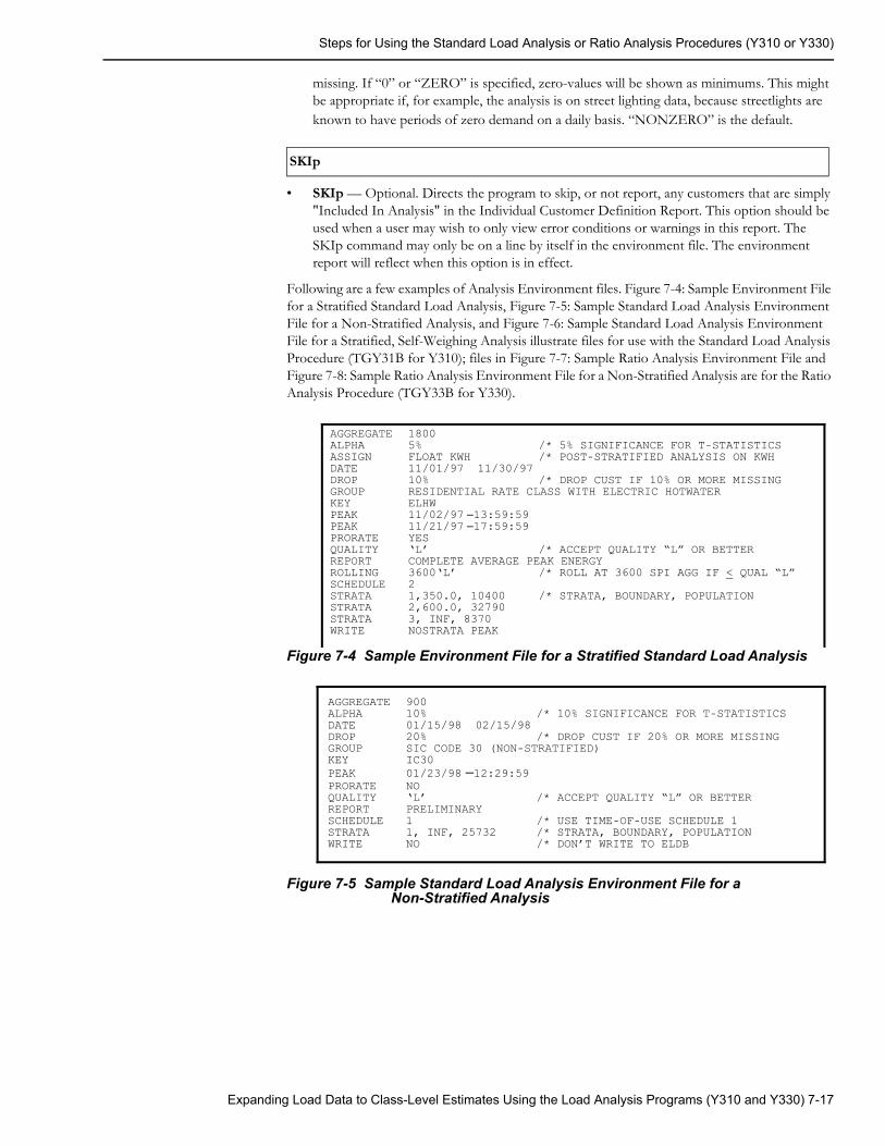
Steps for Using the Standard Load Analysis or Ratio Analysis Procedures (Y310 or Y330)
missing. If “0” or “ZERO” is specified, zero-values will be shown as minimums. This might be appropriate if, for example, the analysis is on street lighting data, because streetlights are known to have periods of zero demand on a daily basis. “NONZERO” is the default.
• SKIp — Optional. Directs the program to skip, or not report, any customers that are simply "Included In Analysis" in the Individual Customer Definition Report. This option should be used when a user may wish to only view error conditions or warnings in this report. The SKIp command may only be on a line by itself in the environment file. The environment report will reflect when this option is in effect.
Following are a few examples of Analysis Environment files. Figure 7-4: Sample Environment File for a Stratified Standard Load Analysis, Figure 7-5: Sample Standard Load Analysis Environment File for a Non-Stratified Analysis, and Figure 7-6: Sample Standard Load Analysis Environment File for a Stratified, Self-Weighing Analysis illustrate files for use with the Standard Load Analysis Procedure (TGY31B for Y310); files in Figure 7-7: Sample Ratio Analysis Environment File and Figure 7-8: Sample Ratio Analysis Environment File for a Non-Stratified Analysis are for the Ratio Analysis Procedure (TGY33B for Y330).
Figure 7-4 Sample Environment File for a Stratified Standard Load Analysis
Figure 7-5 Sample Standard Load Analysis Environment File for a Non-Stratified Analysis
SKIp
AGGREGATE 1800ALPHA 5% /* 5% SIGNIFICANCE FOR T-STATISTICSASSIGN FLOAT KWH /* POST-STRATIFIED ANALYSIS ON KWHDATE 11/01/97 11/30/97DROP 10% /* DROP CUST IF 10% OR MORE MISSINGGROUP RESIDENTIAL RATE CLASS WITH ELECTRIC HOTWATERKEY ELHWPEAK 11/02/97 –13:59:59PEAK 11/21/97 –17:59:59PRORATE YESQUALITY ‘L’ /* ACCEPT QUALITY “L” OR BETTERREPORT COMPLETE AVERAGE PEAK ENERGYROLLING 3600‘L’ /* ROLL AT 3600 SPI AGG IF < QUAL “L”SCHEDULE 2STRATA 1,350.0, 10400 /* STRATA, BOUNDARY, POPULATIONSTRATA 2,600.0, 32790STRATA 3, INF, 8370WRITE NOSTRATA PEAK
AGGREGATE 900ALPHA 10% /* 10% SIGNIFICANCE FOR T-STATISTICSDATE 01/15/98 02/15/98DROP 20% /* DROP CUST IF 20% OR MORE MISSINGGROUP SIC CODE 30 (NON-STRATIFIED)KEY IC30PEAK 01/23/98 –12:29:59PRORATE NOQUALITY ‘L’ /* ACCEPT QUALITY “L” OR BETTERREPORT PRELIMINARYSCHEDULE 1 /* USE TIME-OF-USE SCHEDULE 1STRATA 1, INF, 25732 /* STRATA, BOUNDARY, POPULATIONWRITE NO /* DON’T WRITE TO ELDB
Expanding Load Data to Class-Level Estimates Using the Load Analysis Programs (Y310 and Y330) 7-17
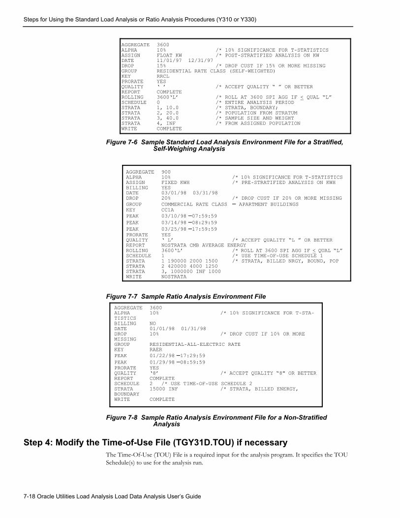
Steps for Using the Standard Load Analysis or Ratio Analysis Procedures (Y310 or Y330)
Figure 7-6 Sample Standard Load Analysis Environment File for a Stratified, Self-Weighing Analysis
Figure 7-7 Sample Ratio Analysis Environment File
Figure 7-8 Sample Ratio Analysis Environment File for a Non-Stratified Analysis
Step 4: Modify the Time-of-Use File (TGY31D.TOU) if necessaryThe Time-Of-Use (TOU) File is a required input for the analysis program. It specifies the TOU Schedule(s) to use for the analysis run.
AGGREGATE 3600ALPHA 10% /* 10% SIGNIFICANCE FOR T-STATISTICSASSIGN FLOAT KW /* POST-STRATIFIED ANALYSIS ON KWDATE 11/01/97 12/31/97DROP 15% /* DROP CUST IF 15% OR MORE MISSINGGROUP RESIDENTIAL RATE CLASS (SELF-WEIGHTED)KEY RRCLPRORATE YESQUALITY ‘ ’ /* ACCEPT QUALITY “ ” OR BETTERREPORT COMPLETEROLLING 3600‘L’ /* ROLL AT 3600 SPI AGG IF < QUAL “L”SCHEDULE 0 /* ENTIRE ANALYSIS PERIODSTRATA 1, 10.0 /* STRATA, BOUNDARY;STRATA 2, 20.0 /* POPULATION FROM STRATUMSTRATA 3, 40.0 /* SAMPLE SIZE AND WEIGHTSTRATA 4, INF /* FROM ASSIGNED POPULATIONWRITE COMPLETE
AGGREGATE 900ALPHA 10% /* 10% SIGNIFICANCE FOR T-STATISTICSASSIGN FIXED KWH /* PRE-STRATIFIED ANALYSIS ON KWHBILLING YESDATE 03/01/98 03/31/98DROP 20% /* DROP CUST IF 20% OR MORE MISSINGGROUP COMMERCIAL RATE CLASS – APARTMENT BUILDINGSKEY CC1APEAK 03/10/98 –07:59:59PEAK 03/14/98 –08:29:59PEAK 03/25/98 –17:59:59PRORATE YESQUALITY ‘ L’ /* ACCEPT QUALITY “L ” OR BETTERREPORT NOSTRATA CMB AVERAGE ENERGYROLLING 3600‘L’ /* ROLL AT 3600 SPI AGG IF < QUAL “L”SCHEDULE 1 /* USE TIME-OF-USE SCHEDULE 1STRATA 1 190000 2000 1500 /* STRATA, BILLED NRGY, BOUND, POPSTRATA 2 420000 4000 1250STRATA 3, 1000000 INF 1000WRITE NOSTRATA
AGGREGATE 3600ALPHA 10% /* 10% SIGNIFICANCE FOR T-STA-TISTICSBILLING NODATE 01/01/98 01/31/98DROP 10% /* DROP CUST IF 10% OR MORE MISSINGGROUP RESIDENTIAL-ALL-ELECTRIC RATEKEY RAERPEAK 01/22/98 –17:29:59PEAK 01/29/98 –08:59:59PRORATE YESQUALITY ‘8’ /* ACCEPT QUALITY “8" OR BETTERREPORT COMPLETESCHEDULE 2 /* USE TIME-OF-USE SCHEDULE 2STRATA 15000 INF /* STRATA, BILLED ENERGY, BOUNDARYWRITE COMPLETE
7-18 Oracle Utilities Load Analysis Load Data Analysis User’s Guide
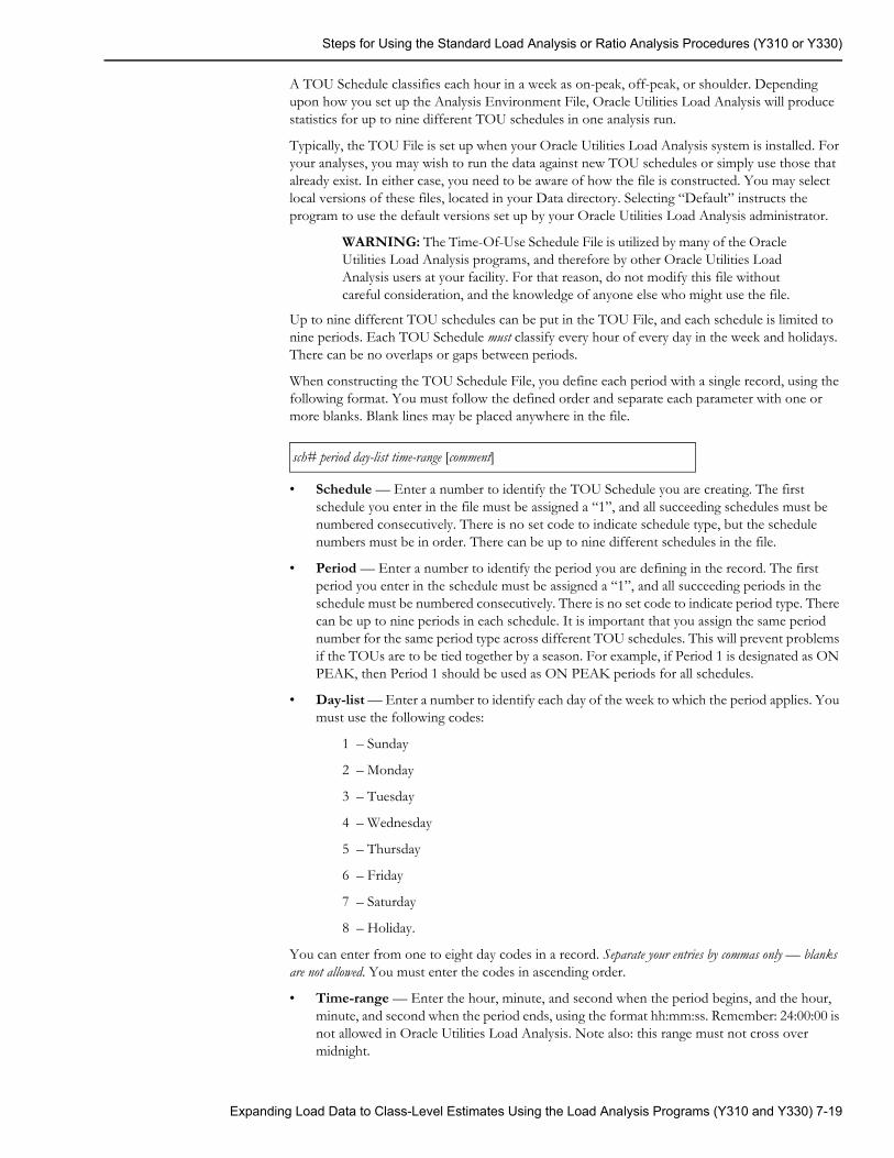
Steps for Using the Standard Load Analysis or Ratio Analysis Procedures (Y310 or Y330)
A TOU Schedule classifies each hour in a week as on-peak, off-peak, or shoulder. Depending upon how you set up the Analysis Environment File, Oracle Utilities Load Analysis will produce statistics for up to nine different TOU schedules in one analysis run.
Typically, the TOU File is set up when your Oracle Utilities Load Analysis system is installed. For your analyses, you may wish to run the data against new TOU schedules or simply use those that already exist. In either case, you need to be aware of how the file is constructed. You may select local versions of these files, located in your Data directory. Selecting “Default” instructs the program to use the default versions set up by your Oracle Utilities Load Analysis administrator.
WARNING: The Time-Of-Use Schedule File is utilized by many of the Oracle Utilities Load Analysis programs, and therefore by other Oracle Utilities Load Analysis users at your facility. For that reason, do not modify this file without careful consideration, and the knowledge of anyone else who might use the file.
Up to nine different TOU schedules can be put in the TOU File, and each schedule is limited to nine periods. Each TOU Schedule must classify every hour of every day in the week and holidays. There can be no overlaps or gaps between periods.
When constructing the TOU Schedule File, you define each period with a single record, using the following format. You must follow the defined order and separate each parameter with one or more blanks. Blank lines may be placed anywhere in the file.
• Schedule — Enter a number to identify the TOU Schedule you are creating. The first schedule you enter in the file must be assigned a “1”, and all succeeding schedules must be numbered consecutively. There is no set code to indicate schedule type, but the schedule numbers must be in order. There can be up to nine different schedules in the file.
• Period — Enter a number to identify the period you are defining in the record. The first period you enter in the schedule must be assigned a “1”, and all succeeding periods in the schedule must be numbered consecutively. There is no set code to indicate period type. There can be up to nine periods in each schedule. It is important that you assign the same period number for the same period type across different TOU schedules. This will prevent problems if the TOUs are to be tied together by a season. For example, if Period 1 is designated as ON PEAK, then Period 1 should be used as ON PEAK periods for all schedules.
• Day-list — Enter a number to identify each day of the week to which the period applies. You must use the following codes:
1 – Sunday
2 – Monday
3 – Tuesday
4 – Wednesday
5 – Thursday
6 – Friday
7 – Saturday
8 – Holiday.
You can enter from one to eight day codes in a record. Separate your entries by commas only — blanks are not allowed. You must enter the codes in ascending order.
• Time-range — Enter the hour, minute, and second when the period begins, and the hour, minute, and second when the period ends, using the format hh:mm:ss. Remember: 24:00:00 is not allowed in Oracle Utilities Load Analysis. Note also: this range must not cross over midnight.
sch# period day-list time-range [comment]
Expanding Load Data to Class-Level Estimates Using the Load Analysis Programs (Y310 and Y330) 7-19
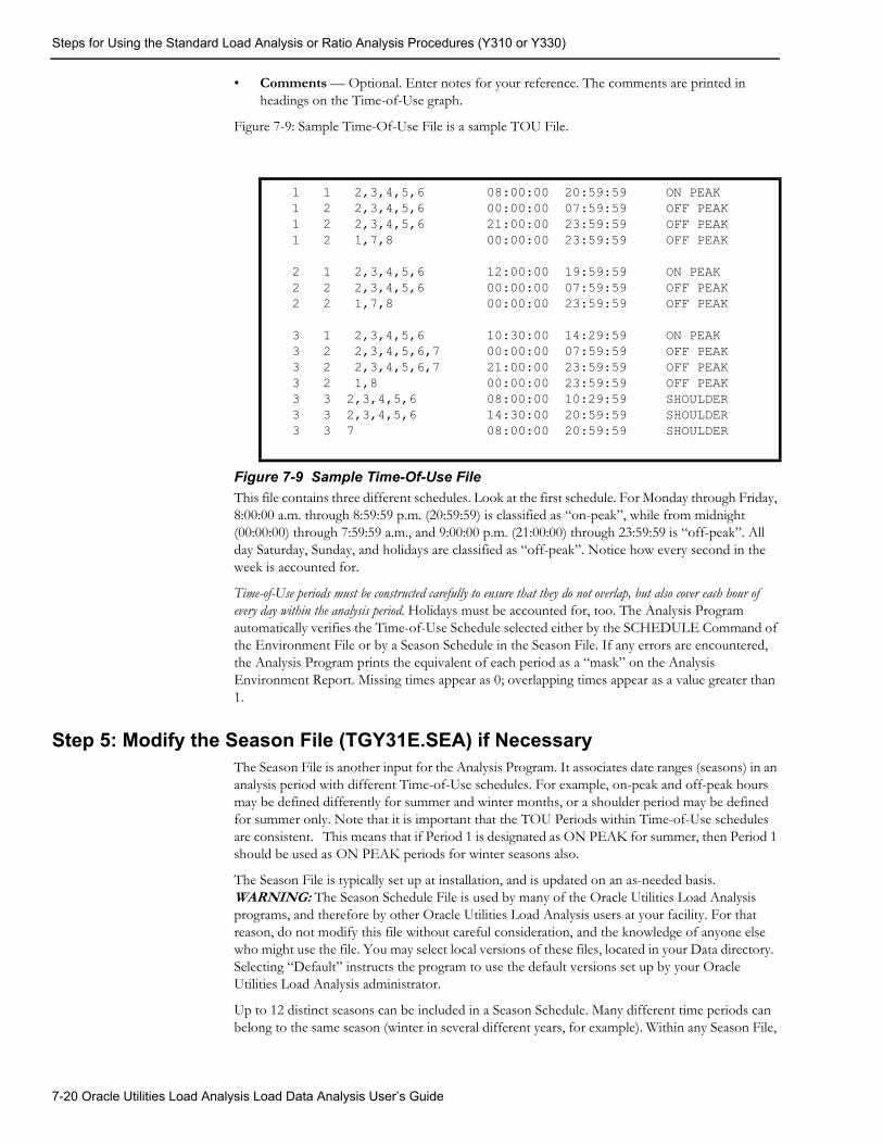
Steps for Using the Standard Load Analysis or Ratio Analysis Procedures (Y310 or Y330)
• Comments — Optional. Enter notes for your reference. The comments are printed in headings on the Time-of-Use graph.
Figure 7-9: Sample Time-Of-Use File is a sample TOU File.
Figure 7-9 Sample Time-Of-Use FileThis file contains three different schedules. Look at the first schedule. For Monday through Friday, 8:00:00 a.m. through 8:59:59 p.m. (20:59:59) is classified as “on-peak”, while from midnight (00:00:00) through 7:59:59 a.m., and 9:00:00 p.m. (21:00:00) through 23:59:59 is “off-peak”. All day Saturday, Sunday, and holidays are classified as “off-peak”. Notice how every second in the week is accounted for.
Time-of-Use periods must be constructed carefully to ensure that they do not overlap, but also cover each hour of every day within the analysis period. Holidays must be accounted for, too. The Analysis Program automatically verifies the Time-of-Use Schedule selected either by the SCHEDULE Command of the Environment File or by a Season Schedule in the Season File. If any errors are encountered, the Analysis Program prints the equivalent of each period as a “mask” on the Analysis Environment Report. Missing times appear as 0; overlapping times appear as a value greater than 1.
Step 5: Modify the Season File (TGY31E.SEA) if NecessaryThe Season File is another input for the Analysis Program. It associates date ranges (seasons) in an analysis period with different Time-of-Use schedules. For example, on-peak and off-peak hours may be defined differently for summer and winter months, or a shoulder period may be defined for summer only. Note that it is important that the TOU Periods within Time-of-Use schedules are consistent. This means that if Period 1 is designated as ON PEAK for summer, then Period 1 should be used as ON PEAK periods for winter seasons also.
The Season File is typically set up at installation, and is updated on an as-needed basis. WARNING: The Season Schedule File is used by many of the Oracle Utilities Load Analysis programs, and therefore by other Oracle Utilities Load Analysis users at your facility. For that reason, do not modify this file without careful consideration, and the knowledge of anyone else who might use the file. You may select local versions of these files, located in your Data directory. Selecting “Default” instructs the program to use the default versions set up by your Oracle Utilities Load Analysis administrator.
Up to 12 distinct seasons can be included in a Season Schedule. Many different time periods can belong to the same season (winter in several different years, for example). Within any Season File,
1 1 2,3,4,5,6 08:00:00 20:59:59 ON PEAK 1 2 2,3,4,5,6 00:00:00 07:59:59 OFF PEAK 1 2 2,3,4,5,6 21:00:00 23:59:59 OFF PEAK 1 2 1,7,8 00:00:00 23:59:59 OFF PEAK 2 1 2,3,4,5,6 12:00:00 19:59:59 ON PEAK 2 2 2,3,4,5,6 00:00:00 07:59:59 OFF PEAK 2 2 1,7,8 00:00:00 23:59:59 OFF PEAK 3 1 2,3,4,5,6 10:30:00 14:29:59 ON PEAK 3 2 2,3,4,5,6,7 00:00:00 07:59:59 OFF PEAK 3 2 2,3,4,5,6,7 21:00:00 23:59:59 OFF PEAK 3 2 1,8 00:00:00 23:59:59 OFF PEAK 3 3 2,3,4,5,6 08:00:00 10:29:59 SHOULDER 3 3 2,3,4,5,6 14:30:00 20:59:59 SHOULDER 3 3 7 08:00:00 20:59:59 SHOULDER
7-20 Oracle Utilities Load Analysis Load Data Analysis User’s Guide

Steps for Using the Standard Load Analysis or Ratio Analysis Procedures (Y310 or Y330)
every time period assigned to the same season must also be associated with the same Time-of-Use Schedule.
There can be no underlaps or gaps between periods. Also, all Time-of-Use schedules referred to in the Season File must be defined in the Time-of-Use Schedule File.
When constructing the Season File, you define each season with a single record, using the following format. You must input the data in the same order as in the format example, and separate each parameter with commas and/or one or more blanks.
• Season-Schedule# — Enter a number to identify the Season Schedule you are creating. The first schedule you enter in the file must be assigned a “1”, and all following schedules must be numbered consecutively. The number of schedules is not limited.
• Season — Enter a number to identify the season you are defining in the record. There can be up to 12 seasons in a schedule.
• TOU-Schedule# — Enter a number to identify the Time-of-Use Schedule (defined in the Time-of-Use File) to be used for this season.
• Date-Range — Enter the date and time when the season begins, and the date and time when the season ends. You can use either “mm/dd/yy-hh:mm:ss” or “mmddyyhhmmss” format. Date ranges must begin at the beginning of a full day. Therefore, the beginning time (hh:mm:ss) must be “00:00:00”, and the ending time must be “23:59:59”. If times other than these are input, they are ignored and “00:00:00” and “23:59:59” are used instead.
All records for each Season Schedule must be grouped together, and season record blocks must be input in ascending order by Season Schedule number. For example, in Figure 7-10: Sample Season File there are seven records associated with Season Schedule number 1, and they precede Season Schedule number 2.
Remember, a Season Schedule selected (via the SEAson Environment File Command) for use in the Analysis Program must contain season segments covering all times in the analysis periods, with no gaps and no overlaps. If the program detects a gap or an overlap in the designated Season Schedule, it will produce an error message and stop processing.
Figure 7-10: Sample Season File illustrates a Season File containing two season schedules, one defining two distinct seasons and the other defining four. Either Season Schedule 1 or Season Schedule 2 could be used for an analysis of the period from July through December of 1992, for example; but only Season Schedule 2 could be used over the same months in 1993.
season-sch# season# tou-sch# date-range [comment]
Expanding Load Data to Class-Level Estimates Using the Load Analysis Programs (Y310 and Y330) 7-21
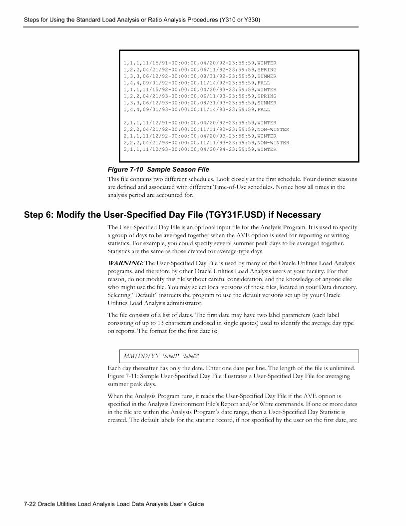
Steps for Using the Standard Load Analysis or Ratio Analysis Procedures (Y310 or Y330)
Figure 7-10 Sample Season FileThis file contains two different schedules. Look closely at the first schedule. Four distinct seasons are defined and associated with different Time-of-Use schedules. Notice how all times in the analysis period are accounted for.
Step 6: Modify the User-Specified Day File (TGY31F.USD) if NecessaryThe User-Specified Day File is an optional input file for the Analysis Program. It is used to specify a group of days to be averaged together when the AVE option is used for reporting or writing statistics. For example, you could specify several summer peak days to be averaged together. Statistics are the same as those created for average-type days.
WARNING: The User-Specified Day File is used by many of the Oracle Utilities Load Analysis programs, and therefore by other Oracle Utilities Load Analysis users at your facility. For that reason, do not modify this file without careful consideration, and the knowledge of anyone else who might use the file. You may select local versions of these files, located in your Data directory. Selecting “Default” instructs the program to use the default versions set up by your Oracle Utilities Load Analysis administrator.
The file consists of a list of dates. The first date may have two label parameters (each label consisting of up to 13 characters enclosed in single quotes) used to identify the average day type on reports. The format for the first date is:
Each day thereafter has only the date. Enter one date per line. The length of the file is unlimited. Figure 7-11: Sample User-Specified Day File illustrates a User-Specified Day File for averaging summer peak days.
When the Analysis Program runs, it reads the User-Specified Day File if the AVE option is specified in the Analysis Environment File’s Report and/or Write commands. If one or more dates in the file are within the Analysis Program’s date range, then a User-Specified Day Statistic is created. The default labels for the statistic record, if not specified by the user on the first date, are
1,1,1,11/15/91-00:00:00,04/20/92-23:59:59,WINTER 1,2,2,04/21/92-00:00:00,06/11/92-23:59:59,SPRING 1,3,3,06/12/92-00:00:00,08/31/92-23:59:59,SUMMER 1,4,4,09/01/92-00:00:00,11/14/92-23:59:59,FALL 1,1,1,11/15/92-00:00:00,04/20/93-23:59:59,WINTER 1,2,2,04/21/93-00:00:00,06/11/93-23:59:59,SPRING 1,3,3,06/12/93-00:00:00,08/31/93-23:59:59,SUMMER 1,4,4,09/01/93-00:00:00,11/14/93-23:59:59,FALL 2,1,1,11/12/91-00:00:00,04/20/92-23:59:59,WINTER 2,2,2,04/21/92-00:00:00,11/11/92-23:59:59,NON-WINTER 2,1,1,11/12/92-00:00:00,04/20/93-23:59:59,WINTER 2,2,2,04/21/93-00:00:00,11/11/93-23:59:59,NON-WINTER 2,1,1,11/12/93-00:00:00,04/20/94-23:59:59,WINTER
MM/DD/YY ‘label1’ ‘label2’
7-22 Oracle Utilities Load Analysis Load Data Analysis User’s Guide
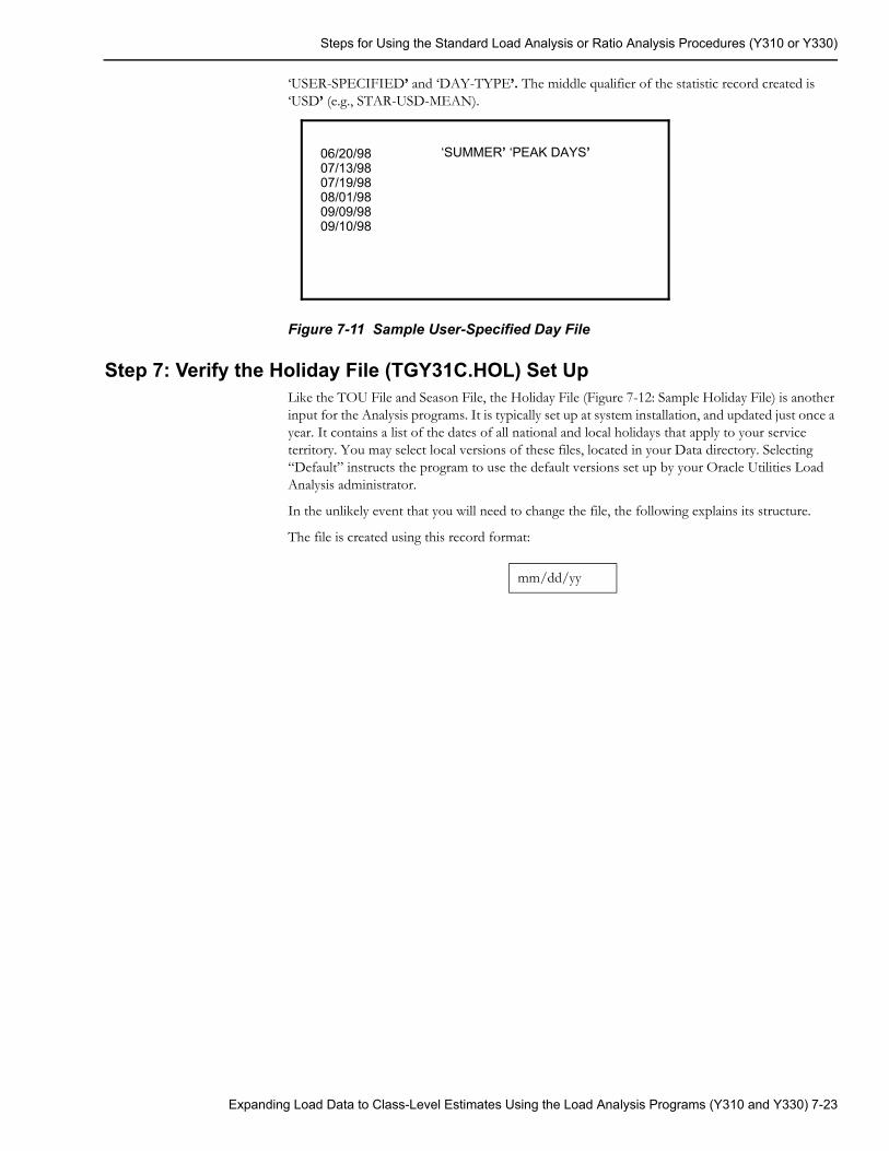
Steps for Using the Standard Load Analysis or Ratio Analysis Procedures (Y310 or Y330)
‘USER-SPECIFIED’ and ‘DAY-TYPE’. The middle qualifier of the statistic record created is ‘USD’ (e.g., STAR-USD-MEAN).
Figure 7-11 Sample User-Specified Day File
Step 7: Verify the Holiday File (TGY31C.HOL) Set UpLike the TOU File and Season File, the Holiday File (Figure 7-12: Sample Holiday File) is another input for the Analysis programs. It is typically set up at system installation, and updated just once a year. It contains a list of the dates of all national and local holidays that apply to your service territory. You may select local versions of these files, located in your Data directory. Selecting “Default” instructs the program to use the default versions set up by your Oracle Utilities Load Analysis administrator.
In the unlikely event that you will need to change the file, the following explains its structure.
The file is created using this record format:
‘SUMMER’ ‘PEAK DAYS’06/20/9807/13/9807/19/9808/01/9809/09/9809/10/98
mm/dd/yy
Expanding Load Data to Class-Level Estimates Using the Load Analysis Programs (Y310 and Y330) 7-23
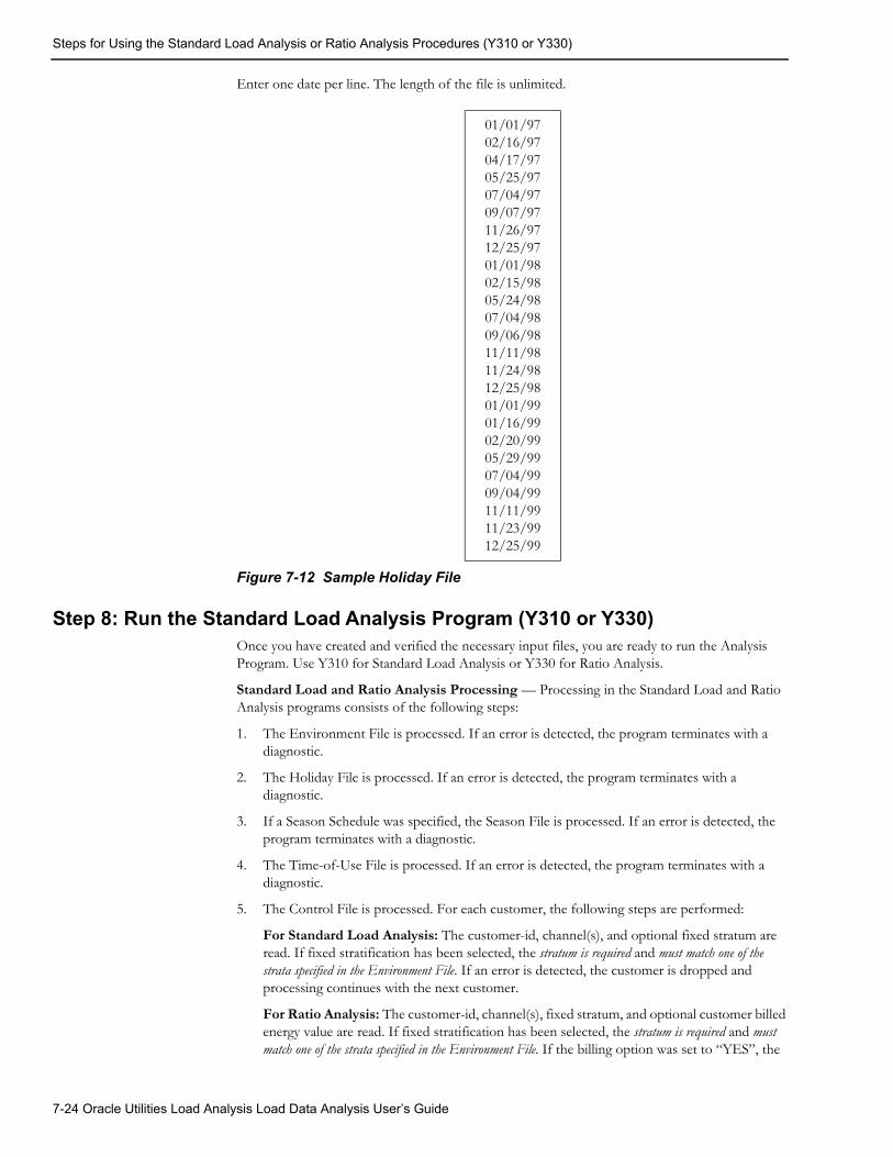
Steps for Using the Standard Load Analysis or Ratio Analysis Procedures (Y310 or Y330)
Enter one date per line. The length of the file is unlimited.
Figure 7-12 Sample Holiday File
Step 8: Run the Standard Load Analysis Program (Y310 or Y330)Once you have created and verified the necessary input files, you are ready to run the Analysis Program. Use Y310 for Standard Load Analysis or Y330 for Ratio Analysis.
Standard Load and Ratio Analysis Processing — Processing in the Standard Load and Ratio Analysis programs consists of the following steps:
1. The Environment File is processed. If an error is detected, the program terminates with a diagnostic.
2. The Holiday File is processed. If an error is detected, the program terminates with a diagnostic.
3. If a Season Schedule was specified, the Season File is processed. If an error is detected, the program terminates with a diagnostic.
4. The Time-of-Use File is processed. If an error is detected, the program terminates with a diagnostic.
5. The Control File is processed. For each customer, the following steps are performed:
For Standard Load Analysis: The customer-id, channel(s), and optional fixed stratum are read. If fixed stratification has been selected, the stratum is required and must match one of the strata specified in the Environment File. If an error is detected, the customer is dropped and processing continues with the next customer.
For Ratio Analysis: The customer-id, channel(s), fixed stratum, and optional customer billed energy value are read. If fixed stratification has been selected, the stratum is required and must match one of the strata specified in the Environment File. If the billing option was set to “YES”, the
01/01/9702/16/9704/17/9705/25/9707/04/9709/07/9711/26/9712/25/9701/01/9802/15/9805/24/9807/04/9809/06/9811/11/9811/24/9812/25/9801/01/9901/16/9902/20/9905/29/9907/04/9909/04/9911/11/9911/23/9912/25/99
7-24 Oracle Utilities Load Analysis Load Data Analysis User’s Guide

Steps for Using the Standard Load Analysis or Ratio Analysis Procedures (Y310 or Y330)
energy values in the Control File are used in the ratio estimates. If an error is detected, the customer is dropped and processing continues with the next customer.
6. If the ROLLING option is selected, the combined channel is converted to rolling average intervals at the specified “window” size. If intervals within a window are below the desired level, they are considered missing and the resulting average is given a status code of ‘5’.
7. The customer’s energy array is scanned for missing data over the entire analysis period. If the number of missing intervals exceeds the drop threshold specified in the Environment File, the customer is dropped and processing continues with the next customer.
8. The customer’s energy array is scanned for missing data on a time-of-use period basis. If all data within any time-of-use period is missing, the customer is dropped and processing continues with the next customer.
9. The following statistics are calculated within each time-of-use period:
• Actual energy
• Prorated energy (if selected) based on the ratio of expected intervals to non-missing intervals
• Non-coincident demand, date and time
• Load factor based on non-coincident demand and average (prorated) demand.
10. The following statistics are calculated for the entire period:
• Actual energy, defined as the sum of time-of-use period actual energies
• Prorated energy (if selected), defined as the sum of time-of-use period prorated energies
• Non-coincident demand, date and time
• Load factor based on non-coincident demand and average (prorated) energy.
11. The following statistics are calculated for each supplied peak:
• Coincident demand
• Load factor based on coincident demand and average (prorated) energy from the entire period
• Diversity factor.
12. If preliminary analysis is selected, processing continues with the next customer; otherwise, the stratification basis is examined. If floating stratification is in effect, the customer’s energy, non-coincident demand, or load factor is compared to the stratum boundary values specified in the Environment File.
13. The customer’s energy array is converted to demand units, and is accumulated into the sum of demands, sum of squared demands, and sample size, for the indicated stratum for each interval in the period.
14. If preliminary analysis is selected, the program skips to the output section for individual customer statistics.
15. The stratum arrays are checked for completeness. If one or more strata is empty, the program issues a diagnostic and skips to the output section. If a stratum sample size exceeds the population specified in the Environment File, the program assumes 100% sampling for the stratum and issues a diagnostic.
16. The following five steps apply to Ratio Analysis only:
• Depending on the billing option selected and the customer’s interval status codes, either the customer’s recorded energy or billed energy is accumulated into a sum of energies and sum of squared energies for the indicated strata for each interval of the period.
Expanding Load Data to Class-Level Estimates Using the Load Analysis Programs (Y310 and Y330) 7-25

Steps for Using the Standard Load Analysis or Ratio Analysis Procedures (Y310 or Y330)
• For the separate ratio estimate, the ratio of mean demand divided by mean energy is calculated for each strata, and these ratios are multiplied by the corresponding stratum’s total billed energy to produce estimates for each strata of the analysis. The individual strata are then summed to obtain total class demand for each interval of the analysis period. The ratio statistic is written to the ELDB (suffix = ’RRAT’).
• For the combined ratio estimate, the ratio is computed by dividing total demand summed over all strata by total energy summed over all strata and multiplying this ratio by total billed energy for the class. This calculation of total class demand is performed for each interval of the analysis period. The combined ratio statistic is written to the ELDB (suffix = ’CRAT’).
• For the non-stratified ratio estimate, the calculation is basically the same as for the combined ratio estimate, except only one strata is involved.
• For each of the above estimates, a different set of tests is performed to determine if the analysis assumptions are correct. The tests are conducted on an interval-by-interval basis for all intervals of the analysis period. If any of these tests is not passed, then for that interval, the ratio estimate and associated statistics computed may not yield accurate results.
17. The strata statistics for coincident demands are computed according to the methodology listed in Appendix B: Analysis Equations. A sample evaluation report is printed for the entire period, and the coincident demand statistics are written to the ELDB.
18. The maximum and minimum demands and the dates and times are computed over the entire period, by time-of-use, for supplied peaks (no minimum), and for strata peaks.
19. Coincident demands are computed, reported, and written to the ELDB for the following types of days:
• Average day
• Average day, excluding holiday
• Average weekday
• Average weekday, excluding holiday
• Average weekend
• Average weekend including holidays
• Average weekend, excluding holidays
• Average Sunday, Monday,..., Saturday
• Weekday holiday (if available)
• Weekend holiday (if available)
• Average User-Specified Day (if available)
• Days of maximum demands (entire period, and by time-of-use)
• Days of minimum demands (entire period, and by time-of-use)
• Days of supplied peaks (if available).
20. Individual customer coincident demands are retrieved for the strata peak, and for class peak over the entire period and by time-of-use. Customer load factors and diversity factors are also computed.
The following class, sample, and strata statistics are computed from the individual customer statistics:
• Non-coincident demand
• Energy
7-26 Oracle Utilities Load Analysis Load Data Analysis User’s Guide
Steps for Using the Standard Load Analysis or Ratio Analysis Procedures (Y310 or Y330)
• Load factor based on maximum coincident demand
• Load factor based on non-coincident demand
• Diversity factor
• Coincidence factor
• Standard deviation of residuals of demand (sample and strata only).
The above statistics are reported and written to the ELDB. For both preliminary and complete analysis, the individual customer statistics are reported and written to a sequential file.The statistics written to the ELDB may also be exported to a graph file.
Bias Tests — Ratio OnlyThere are two types of checks on the accuracy of the analysis estimates. First, due to a small sample size, the large sample formula for the estimated variance of the ratio estimates may be an underestimate. This will make the estimates appear more accurate than they really are. Second, because of the tendency for the ratio estimates to be biased, a test is performed to ensure that the bias is negligible. In practice the bias isn’t important in large or moderate size samples. However, for small samples and in stratified sampling with many strata, the bias can be significant. A large bias can cause a ratio estimate of the mean load to be substantially different from the true population mean.
• In a non-stratified ratio analysis three separate tests are performed to ensure accurate estimation results. These consist of a sample size test and two tests for bias. The sample size test checks to see if the sample size for every interval of the analysis period is 30 customers or more. If the sample size is below 30, an “N” (for “Not 30 or more customers”) is printed in the Bias Flag field, warning that the sample size may be too low for the large sample variance formula to be applicable. Two bias tests are also performed, one based on energy and one based on demand. The energy bias test compares the coefficient of variation of energy (the ratio of the standard error of the sample mean energy divided by the sample mean energy) to the value 0.2, a cutoff level for bias based on empirical research. If the coefficient of variation for energy is greater than or equal to 0.2, the estimates may suffer due to biased results, and an “E” (for “Energy test results may be biased”) is printed in the Bias Flag field. A similar bias test is applied to demand using its coefficient of variation, with a “D” (for “Demand”) being printed if this test fails. These three tests are performed in the order stated above. Whenever a test fails, none of the succeeding tests are performed and the flag printed represents only the failed test.
• In a combined ratio analysis only two tests are done. They are the sample size test (with “N” indicating failure) and the energy bias test (where an “E” indicates failure). For the sample size test, the total sample size for the combined strata is tested against the cutoff value of thirty. The energy bias test is the same as the one used in the non-stratified analysis, and the same considerations and interpretations are applicable.
• In a separate ratio analysis, two tests are also performed to test sample size and the energy bias. The sample size test is the same as the one employed in both non-stratified and combined ratio analysis. The energy bias test is different from those already mentioned, because it tests the square root of the product of the number of strata multiplied by the coefficient of variation for energy, against a cutoff of 0.6. This larger value for the cutoff reflects the fact that the bias calculation includes an accumulated value over all strata, and therefore a larger value can be tolerated and still result in negligible bias. If this test fails, an “S” (for “failure of the Separate ratio analysis”) is placed in the Bias Flag field.
The appearance of a Bias Flag for a number of intervals in any ratio analysis does not mean the results are invalid. It should be interpreted as a potential problem that can lower the accuracy and precision of the resultant calculations, but it does not invalidate the analysis. Analysts should carefully consider the results obtained and try to correct the deficiencies in their data, if possible. For more information on all these tests and their impact on the ratio estimates produced, see Chapter 6 of Cochran’s book, Sampling Techniques, 3rd edition, John Wiley and Sons publishers, 1977.
Expanding Load Data to Class-Level Estimates Using the Load Analysis Programs (Y310 and Y330) 7-27
Steps for Using the Standard Load Analysis or Ratio Analysis Procedures (Y310 or Y330)
Step 9: Check OutputAt the end of a run, both the Standard Load Analysis and Ratio Analysis programs produce five outputs: analysis reports, statistics written to the ELDB (or alternate tableset), the Individual Customer Statistics File, the Keylist File, and the Written Key File.
• ELDB Statistics — Unless you specified the “WRITE NO” option in the Analysis Environment file, the program will write all statistics back to the ELDB, saving them for further reporting and analysis. The statistics are stored as simulated cuts with statistics identifiers (see Statistics Records on page 3-8 for an explanation of these IDs). At the end of a run, the program produces a list of all of the statistics written to the tableset in a report entitled “Analysis Statistics Written to the ELDB”. Both the format of this report and the IDs of all possible types of statistics produced by the programs are summarized in Appendix D: Reading “Analysis Statistics Written to the ELDB” Reports and Listings of Analysis Statistic Names of this manual.
• Individual Customer Statistics File — This file (TGY318.DAT) is optionally produced at the end of each successful analysis run. It is a sequential file containing the basic load statistics for each customer in the analysis, and can be used for further analyses with external programs. You have three options for handling this file:
• Write it to a dummy file so that it is not saved, conserving space in the tableset
• Write it over an existing file at the end of each analysis run
• Save it as a catalogued file, preserving the file for further use.
Note: Appendix E: Individual Customer Statistics File Formats details the contents and format of the Individual Customer Statistics File.
• Keylist File — This file (TGY317.DAT) is automatically produced at the end of each successful analysis run. It is a sequential file containing a list of keys (customer-id, channel) of records that were requested but not included in the analysis. This file can be used as a Control File for running subsequent Oracle Utilities Load Analysis programs, such as the Summary Report, to diagnose why the key was excluded.
• Written Key File — This file (KEYLIST.DAT) is produced at the end of each successful analysis run. It is a sequential file containing a list of keys (customer-id, channel, start-time).
7-28 Oracle Utilities Load Analysis Load Data Analysis User’s Guide
Chapter 8Computing Statistics for 100% Sampled
Populations (Y380)
This chapter explains how to use the 100% Sample Analysis Program to compute load statistics for 100% sampled populations such as large industrials. Topics in this chapter are:
• What Does the 100% Sample Analysis Program Do?
• Steps for Using the 100% Sample Analysis Program (Y380)
Computing Statistics for 100% Sampled Populations (Y380) 8-1
What Does the 100% Sample Analysis Program Do?
What Does the 100% Sample Analysis Program Do?The 100% Sample Analysis Program is used to compute load statistics for 100% sampled populations such as large industrials. It allows a variable population and may optionally perform a stratified analysis (fixed strata only). The program does not perform an expansion. It assumes that missing intervals mean that a customer left the system and the population is less. The analysis program requires users to estimate missing data for customers who are part of the sample. There is no need for expansion because the class is 100% sampled. This is the only accurate way to analyze samples of the largest and most diverse customers.
This program analyzes periods of up to a year. Based on the information provided by the input files, the 100% Sample Analysis Program computes coincident demands, non-coincident demands, energy, load factors, and diversity factors. These statistics are provided for the customer and population levels within an analysis group. Statistics are also calculated by time-of-use period, and, in some cases, by type of day. Means and standard deviations are computed for sample evaluation. Most of the statistics are reported and written to the ELDB for additional evaluation and reporting. These statistics may be archived to the SLDB.
100% Sample Analysis also creates a file of individual customer statistics that may be accessed by user programs.
Steps for Using the 100% Sample Analysis Program (Y380)Here is a brief list of the steps you will follow when analyzing load data for 100% sampled populations (Figure 8-1: Overview of the 100% Sample Analysis Program). The remainder of this chapter explains these steps in detail.
Note: The Y310 program supports pre-process key generator. See Using the Key Generator Preprocessor in a Control File on page 4-4 and the Sample Manager for more information.
Summary - Using 100% Sample Analysis
1. Make sure that the tableset (CLDB or ELDB) contains load data for all customers who are part of the sample.
2. Create the Analysis Control File (TGY38A.CTL) - a list of the customers to be analyzed and, if using fixed strata analysis, the strata to which they should be assigned.
3. Create the Analysis Environment File (TGY38B.ENV) - a group of commands that you use to set analysis and reporting options.
4. Verify or modify other required input files:
Time-of-Use Schedule File (TGY31D.TOU)
Season Schedule File (TGY31E.SEA)
User-Specified Day File (TGY31F.USD)
Holiday File (TGY31C.HOL).
5. Run the 100% Sample Analysis Program (Y380).
8-2 Oracle Utilities Load Analysis Load Data Analysis User’s Guide
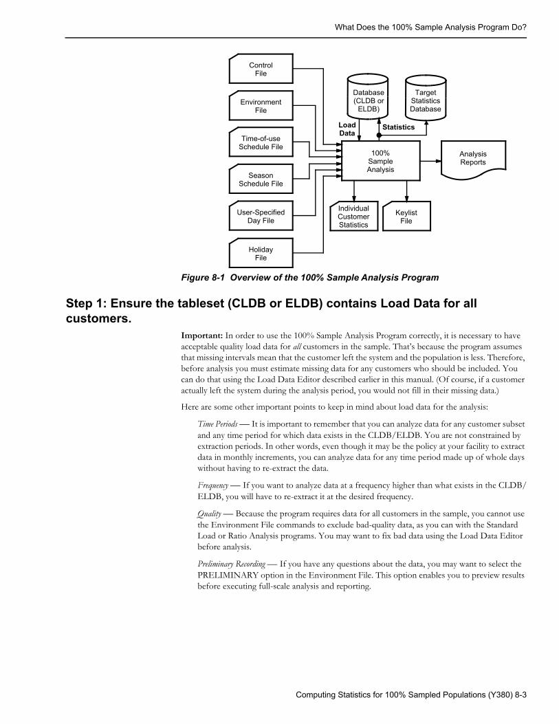
What Does the 100% Sample Analysis Program Do?
Figure 8-1 Overview of the 100% Sample Analysis Program
Step 1: Ensure the tableset (CLDB or ELDB) contains Load Data for all customers.
Important: In order to use the 100% Sample Analysis Program correctly, it is necessary to have acceptable quality load data for all customers in the sample. That’s because the program assumes that missing intervals mean that the customer left the system and the population is less. Therefore, before analysis you must estimate missing data for any customers who should be included. You can do that using the Load Data Editor described earlier in this manual. (Of course, if a customer actually left the system during the analysis period, you would not fill in their missing data.)
Here are some other important points to keep in mind about load data for the analysis:
Time Periods — It is important to remember that you can analyze data for any customer subset and any time period for which data exists in the CLDB/ELDB. You are not constrained by extraction periods. In other words, even though it may be the policy at your facility to extract data in monthly increments, you can analyze data for any time period made up of whole days without having to re-extract the data.
Frequency — If you want to analyze data at a frequency higher than what exists in the CLDB/ELDB, you will have to re-extract it at the desired frequency.
Quality — Because the program requires data for all customers in the sample, you cannot use the Environment File commands to exclude bad-quality data, as you can with the Standard Load or Ratio Analysis programs. You may want to fix bad data using the Load Data Editor before analysis.
Preliminary Recording — If you have any questions about the data, you may want to select the PRELIMINARY option in the Environment File. This option enables you to preview results before executing full-scale analysis and reporting.
SeasonSchedule File
User-Specified Day File
100%SampleAnalysis
AnalysisReports
IndividualCustomerStatistics
KeylistFile
Database(CLDB or
ELDB)
StatisticsLoadData
ControlFile
HolidayFile
EnvironmentFile
Time-of-useSchedule File
TargetStatisticsDatabase
Computing Statistics for 100% Sampled Populations (Y380) 8-3
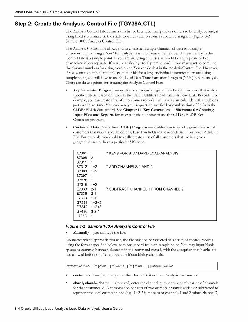
What Does the 100% Sample Analysis Program Do?
Step 2: Create the Analysis Control File (TGY38A.CTL)The Analysis Control File consists of a list of keys identifying the customers to be analyzed and, if using fixed strata analysis, the strata to which each customer should be assigned. (Figure 8-2: Sample 100% Analysis Control File).
The Analysis Control File allows you to combine multiple channels of data for a single customer-id into a single “cut” for analysis. It is important to remember that each entry in the Control File is a sample point. If you are analyzing end uses, it would be appropriate to keep channel-numbers separate. If you are analyzing “total premise loads”, you may want to combine the channel-numbers for a single customer. You can do that in the Analysis Control File. However, if you want to combine multiple customer-ids for a large individual customer to create a single sample point, you will have to use the Load Data Transformation Program (Y620) before analysis. There are three options for creating the Analysis Control File:
• Key Generator Program — enables you to quickly generate a list of customers that match specific criteria, based on fields in the Oracle Utilities Load Analysis Load Data Records. For example, you can create a list of all customer records that have a particular identifier code or a particular start-time. You can base your request on any field or combination of fields in the CLDB/ELDB data record. See Chapter 14: Key Generators — Shortcuts for Creating Input Files and Reports for an explanation of how to use the CLDB/ELDB Key Generator program.
• Customer Data Extraction (CDE) Program — enables you to quickly generate a list of customers that match specific criteria, based on fields in the user-defined Customer Attribute File. For example, you could typically create a list of all customers that are in a given geographic area or have a particular SIC code.
Figure 8-2 Sample 100% Analysis Control File• Manually – you can type the file.
No matter which approach you use, the file must be constructed of a series of control records using the format specified below, with one record for each sample point. You may input blank spaces or commas between elements in the command record, with the exception that blanks are not allowed before or after an operator if combining channels.
• customer-id — (required) enter the Oracle Utilities Load Analysis customer-id
• chan1, chan2...chanx — (required) enter the channel-number or a combination of channels for that customer-id. A combination consists of two or more channels added or subtracted to represent the total customer load (e.g., 1+2-7 is the sum of channels 1 and 2 minus channel 7,
customer-id chan1 [{±}chan2 [{±}chan3...[{±}chann ] ] ] [stratum-number]
A7301 1 /* KEYS FOR STANDARD LOAD ANALYSISB7308 2B7311 1B7312 1+2 /* ADD CHANNELS 1 AND 2B7393 1+2B7397 1C7378 1D7316 1+2E7333 2-1 /* SUBTRACT CHANNEL 1 FROM CHANNEL 2E7336 2-1F7338 1+2G7339 1+2+3G7342 1+2+3G7480 3-2-1L7353 1
8-4 Oracle Utilities Load Analysis Load Data Analysis User’s Guide
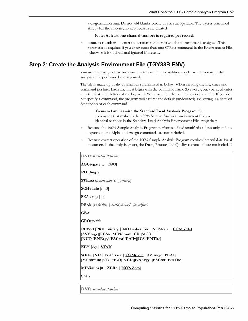
What Does the 100% Sample Analysis Program Do?
a co-generation unit. Do not add blanks before or after an operator. The data is combined strictly for the analysis; no new records are created.
Note: At least one channel-number is required per record.
• stratum-number — enter the stratum number to which the customer is assigned. This parameter is required if you enter more than one STRata command in the Environment File; otherwise it is optional and ignored if present.
Step 3: Create the Analysis Environment File (TGY38B.ENV)You use the Analysis Environment File to specify the conditions under which you want the analysis to be performed and reported.
The file is made up of the commands summarized in below. When creating the file, enter one command per line. Each line must begin with the command name (keyword); but you need enter only the first three letters of the keyword. You may enter the commands in any order. If you do not specify a command, the program will assume the default (underlined). Following is a detailed description of each command.
To users familiar with the Standard Load Analysis Program: the commands that make up the 100% Sample Analysis Environment File are identical to those in the Standard Load Analysis Environment File, except that:
• Because the 100% Sample Analysis Program performs a fixed stratified analysis only and no expansion, the Alpha and Assign commands are not included.
• Because correct operation of the 100% Sample Analysis Program requires interval data for all customers in the analysis group, the Drop, Prorate, and Quality commands are not included.
DATe start-date stop-date
AGGregate [n | 3600]
ROLling n
STRata stratum-number [comment]
SCHedule [t | 0]
SEAson [s | 0]
PEAk {peak-time | custid channel} [descriptor]
GRA
GROup title
REPort [PREliminary | NOEvaluation | NOStrata | COMplete] [AVErage][PEAk][MINimum][CD][MCD] [NCD][ENErgy][FACtor][DAIly][ICS][ENTire]
KEY [key | STAR]
WRIte [NO | NOStrata | COMplete] [AVErage][PEAk] [MINimum][CD][MCD][NCD][ENErgy] [FACtor][ENTire]
MINinum [0 | ZERo | NONZero]
SKIp
DATe start-date stop-date
Computing Statistics for 100% Sampled Populations (Y380) 8-5
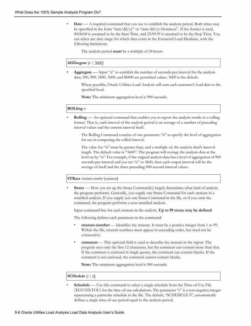
What Does the 100% Sample Analysis Program Do?
• Date — A required command that you use to establish the analysis period. Both times may be specified in the form “mm/dd/yy” or “mm/dd/yy-hh:mm:ss”. If the former is used, 00:00:00 is assumed to be the Start Time, and 23:59:59 is assumed to be the Stop Time. You can select any date range for which data exists in the Extracted Load Database, with the following limitations:
The analysis period must be a multiple of 24 hours.
• Aggregate — Input “n” to establish the number of seconds-per-interval for the analysis data; 300, 900, 1800, 3600, and 86400 are permitted values. 3600 is the default.
Where possible, Oracle Utilities Load Analysis will sum each customer’s load data to the specified level.
Note: The minimum aggregation level is 900 seconds.
• Rolling — An optional command that enables you to report the analysis results in a rolling format. That is, each interval of the analysis period is an average of a number of preceding interval values and the current interval itself.
The Rolling Command consists of one parameter “n” to specify the level of aggregation for use in computing the rolled interval.
The value for “n” must be greater than, and a multiple of, the analysis data’s interval length. The default value is “3600”. The program will average the analysis data at the level set by “n”. For example, if the original analysis data has a level of aggregation of 900 seconds-per-interval and you set “n” to 3600, then each output interval will be the average of itself and the three preceding 900-second interval values.
• Strata — How you set up the Strata Command(s) largely determines what kind of analysis the program performs. Generally, you supply one Strata Command for each stratum in a stratified analysis. If you supply just one Strata Command in the file, or if you omit the command, the program performs a non-stratified analysis.
Input command line for each stratum in the analysis. Up to 99 strata may be defined.
The following defines each parameter in the command:
• stratum-number — Identifies the stratum. It must be a positive integer from 1 to 99. Within the file, stratum numbers must appear in ascending order, but need not be consecutive.
• comment — This optional field is used to describe the stratum in the report. The program uses only the first 12 characters, but the comment can contain more than that. If the comment is enclosed in single quotes, the comment can contain blanks. If the comment is not enclosed, the comment cannot contain blanks.
Note: The minimum aggregation level is 900 seconds.
• Schedule — Use this command to select a single schedule from the Time-of-Use File (TGY31D.TOU) for the time-of-use calculations. The parameter “t” is a non-negative integer representing a particular schedule in the file. The default, “SCHEDULE 0”, automatically defines a single time-of-use period equal to the analysis period.
AGGregate [n | 3600]
ROLling n
STRata stratum-number [comment]
SCHedule [t | 0]
8-6 Oracle Utilities Load Analysis Load Data Analysis User’s Guide
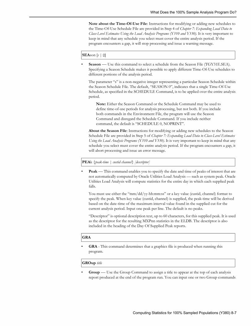
What Does the 100% Sample Analysis Program Do?
Note about the Time-Of-Use File: Instructions for modifying or adding new schedules to the Time-Of-Use Schedule File are provided in Step 4 of Chapter 7: Expanding Load Data to Class-Level Estimates Using the Load Analysis Programs (Y310 and Y330). It is very important to keep in mind that any schedule you select must cover the entire analysis period. If the program encounters a gap, it will stop processing and issue a warning message.
• Season — Use this command to select a schedule from the Season File (TGY31E.SEA). Specifying a Season Schedule makes it possible to apply different Time-Of-Use schedules to different portions of the analysis period.
The parameter “s” is a non-negative integer representing a particular Season Schedule within the Season Schedule File. The default, “SEASON 0”, indicates that a single Time-Of-Use Schedule, as specified in the SCHEDULE Command, is to be applied over the entire analysis period.
Note: Either the Season Command or the Schedule Command may be used to define time-of-use periods for analysis processing, but not both. If you include both commands in the Environment File, the program will use the Season Command and disregard the Schedule Command. If you include neither command, the default is “SCHEDULE 0, NOPRINT”.
About the Season File: Instructions for modifying or adding new schedules to the Season Schedule File are provided in Step 5 of Chapter 7: Expanding Load Data to Class-Level Estimates Using the Load Analysis Programs (Y310 and Y330). It is very important to keep in mind that any schedule you select must cover the entire analysis period. If the program encounters a gap, it will abort processing and issue an error message.
• Peak — This command enables you to specify the date and time of peaks of interest that are not automatically computed by Oracle Utilities Load Analysis — such as system peak. Oracle Utilities Load Analysis will compute statistics for the entire day in which each supplied peak falls.
You must use either the “mm/dd/yy-hh:mm:ss” or a key value (custid, channel) format to specify the peak. When key value (custid, channel) is supplied, the peak-time will be derived based on the date-time of the maximum interval value found in the supplied cut for the current analysis period. Input one peak per line. The default is no peaks.
“Descriptor” is optional description text, up to 60 characters, for this supplied peak. It is used as the descriptor for the resulting MXPnn statistics in the ELDB. The descriptor is also included in the heading of the Day Of Supplied Peak reports.
• GRA - This command determines that a graphics file is produced when running this program.
• Group — Use the Group Command to assign a title to appear at the top of each analysis report produced at the end of the program run. You can input one or two Group commands
SEAson [s | 0]
PEAk {peak-time | custid channel} [descriptor]
GRA
GROup title
Computing Statistics for 100% Sampled Populations (Y380) 8-7
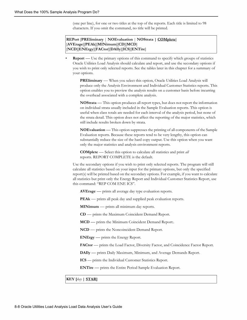
What Does the 100% Sample Analysis Program Do?
(one per line), for one or two titles at the top of the reports. Each title is limited to 98 characters. If you omit the command, no title will be printed.
• Report — Use the primary options of this command to specify which groups of statistics Oracle Utilities Load Analysis should calculate and report, and use the secondary options if you wish to print only selected reports. See the tables later in this chapter for a summary of your options.
PREliminary — When you select this option, Oracle Utilities Load Analysis will produce only the Analysis Environment and Individual Customer Statistics reports. This option enables you to preview the analysis results on a customer basis before incurring the overhead associated with a complete analysis.
NOStrata — This option produces all report types, but does not report the information on individual strata usually included in the Sample Evaluation reports. This option is useful when class totals are needed for each interval of the analysis period, but none of the strata detail. This option does not affect the reporting of the major statistics, which still include results broken down by strata.
NOEvaluation — This option suppresses the printing of all components of the Sample Evaluation reports. Because these reports tend to be very lengthy, this option can substantially reduce the size of the hard copy output. Use this option when you want only the major statistics and analysis environment reports.
COMplete — Select this option to calculate all statistics and print all reports. REPORT COMPLETE is the default.
Use the secondary options if you wish to print only selected reports. The program will still calculate all statistics based on your input for the primary options, but only the specified report(s) will be printed based on the secondary options. For example, if you want to calculate all statistics but print only the Energy Report and Individual Customer Statistics Report, use this command: “REP COM ENE ICS”.
AVErage — prints all average day type evaluation reports.
PEAk — prints all peak day and supplied peak evaluation reports.
MINimum — prints all minimum day reports.
CD — prints the Maximum Coincident Demand Report.
MCD — prints the Minimum Coincident Demand Report:.
NCD — prints the Noncoincident Demand Report.
ENErgy — prints the Energy Report.
FACtor — prints the Load Factor, Diversity Factor, and Coincidence Factor Report.
DAIly — prints Daily Maximum, Minimum, and Average Demands Report.
ICS — prints the Individual Customer Statistics Report.
ENTire — prints the Entire Period Sample Evaluation Report.
REPort [PREliminary | NOEvaluation | NOStrata | COMplete] [AVErage][PEAk][MINimum][CD][MCD] [NCD][ENErgy][FACtor][DAIly][ICS][ENTire]
KEY [key | STAR]
8-8 Oracle Utilities Load Analysis Load Data Analysis User’s Guide
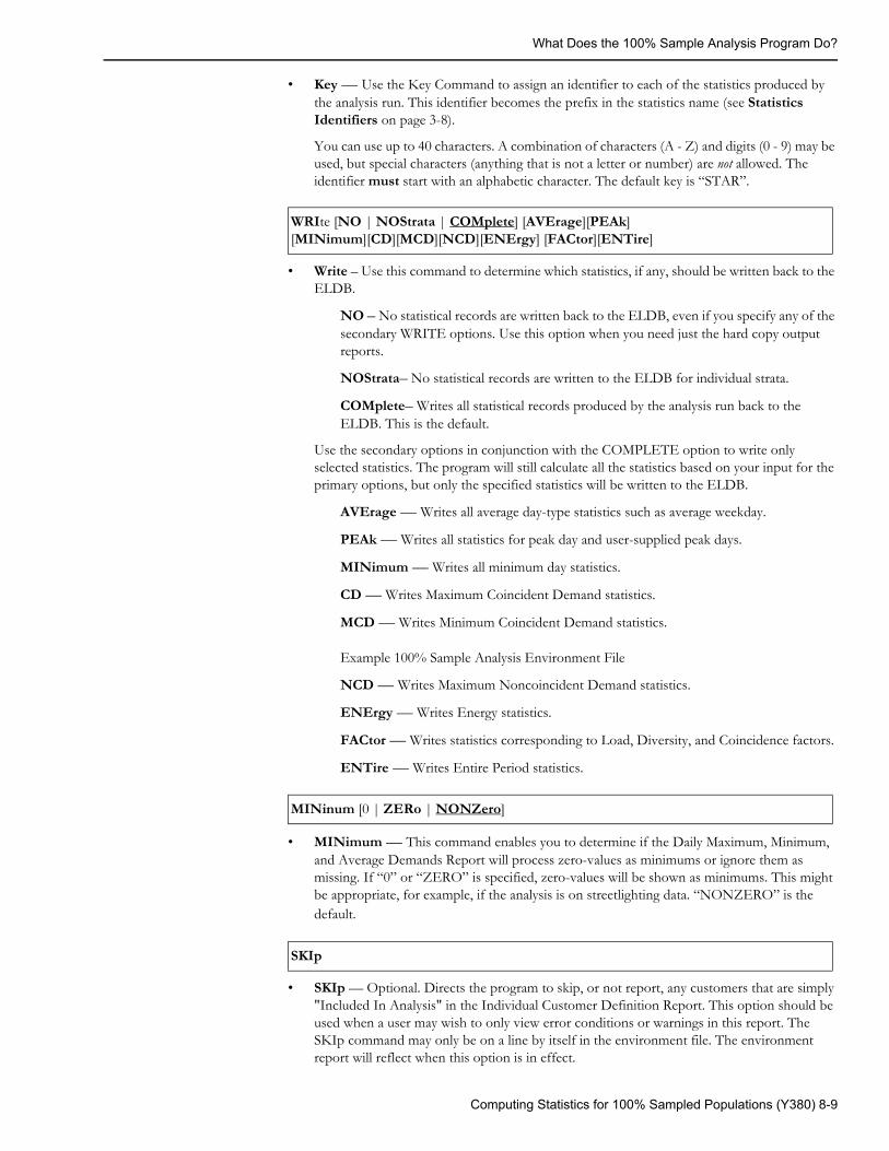
What Does the 100% Sample Analysis Program Do?
• Key — Use the Key Command to assign an identifier to each of the statistics produced by the analysis run. This identifier becomes the prefix in the statistics name (see Statistics Identifiers on page 3-8).
You can use up to 40 characters. A combination of characters (A - Z) and digits (0 - 9) may be used, but special characters (anything that is not a letter or number) are not allowed. The identifier must start with an alphabetic character. The default key is “STAR”.
• Write – Use this command to determine which statistics, if any, should be written back to the ELDB.
NO – No statistical records are written back to the ELDB, even if you specify any of the secondary WRITE options. Use this option when you need just the hard copy output reports.
NOStrata– No statistical records are written to the ELDB for individual strata.
COMplete– Writes all statistical records produced by the analysis run back to the ELDB. This is the default.
Use the secondary options in conjunction with the COMPLETE option to write only selected statistics. The program will still calculate all the statistics based on your input for the primary options, but only the specified statistics will be written to the ELDB.
AVErage — Writes all average day-type statistics such as average weekday.
PEAk — Writes all statistics for peak day and user-supplied peak days.
MINimum — Writes all minimum day statistics.
CD — Writes Maximum Coincident Demand statistics.
MCD — Writes Minimum Coincident Demand statistics.
Example 100% Sample Analysis Environment File
NCD — Writes Maximum Noncoincident Demand statistics.
ENErgy — Writes Energy statistics.
FACtor — Writes statistics corresponding to Load, Diversity, and Coincidence factors.
ENTire — Writes Entire Period statistics.
• MINimum — This command enables you to determine if the Daily Maximum, Minimum, and Average Demands Report will process zero-values as minimums or ignore them as missing. If “0” or “ZERO” is specified, zero-values will be shown as minimums. This might be appropriate, for example, if the analysis is on streetlighting data. “NONZERO” is the default.
• SKIp — Optional. Directs the program to skip, or not report, any customers that are simply "Included In Analysis" in the Individual Customer Definition Report. This option should be used when a user may wish to only view error conditions or warnings in this report. The SKIp command may only be on a line by itself in the environment file. The environment report will reflect when this option is in effect.
WRIte [NO | NOStrata | COMplete] [AVErage][PEAk] [MINimum][CD][MCD][NCD][ENErgy] [FACtor][ENTire]
MINinum [0 | ZERo | NONZero]
SKIp
Computing Statistics for 100% Sampled Populations (Y380) 8-9
What Does the 100% Sample Analysis Program Do?
•
Step 4: Verify or modify other Required Input FilesAlong with the Control and Environment files, four other input files may be required for a 100% Sample Analysis (depending upon your selections in the Environment File):
• Holiday File (TGY31C.HOL) is a list of holidays observed in your service territory.
• Time-of-Use Schedule File (TGY31D.TOU) is a series of TOU schedules.
• Season Schedule File (TGY31E.SEA) is a series of Season schedules that enable you to apply different TOU schedules at different times of the year.
• User-Specified Day File (TGY31F.USD) specifies a group of contiguous or non-contiguous days that may be averaged together for analysis (for example, a set of summer peak days).
Typically, these files are established at system installation and seldom modified. Should you need to update or modify these files (if you want to experiment with a new Time-Of-Use Schedule, for example) see steps 4 - 7 of Chapter 7: Expanding Load Data to Class-Level Estimates Using the Load Analysis Programs (Y310 and Y330). Alternately, you may select local versions of these files, located in your Data directory. Selecting “Default” instructs the program to use the default versions set up by your Oracle Utilities Load Analysis administrator.
Step 5: Run the 100% Sample Analysis Program (Y380)Once you have created and verified the necessary input files, you are ready to run the Analysis Program. Use Y380.
100% Sample Analysis Processing: For your information, processing in the 100% Sample Analysis Program consists of the following steps:
• The Environment File is processed. If an error is detected, the program terminates with a diagnostic.
• The Holiday File is processed. If an error is detected, the program terminates with a diagnostic.
• If a Season Schedule was specified, the Season File is processed. If an error is detected, the program terminates with a diagnostic.
• The Time-of-Use File is processed. If an error is detected, the program terminates with a diagnostic.
• The Control File is processed. For each customer, the following steps are performed:
The customer-id and channel(s) are read. If an error is detected, the customer is dropped and processing continues with the next customer.
The indicated channel(s) is retrieved from the CLDB/ELDB for the analysis period and aggregated accordingly. If an aggregated interval is incomplete, it is assigned a status code of ‘7’. Each channel is converted to energy units and, if necessary, combined. Combined intervals are assigned the worst of the component status codes; incomplete combined intervals are assigned a status code of ‘7’. If one or more channels is missing in its entirety, the customer is dropped, and processing continues with the next customer.
• The customer’s energy array is scanned for missing data on a time-of-use period basis. If all data within any time-of-use period is missing, the customer is dropped and processing continues with the next customer.
The following statistics are calculated within each time-of-use period:
Actual energy
Non-coincident demand, date and time
8-10 Oracle Utilities Load Analysis Load Data Analysis User’s Guide

What Does the 100% Sample Analysis Program Do?
Load factor based on non-coincident demand and average demand.
• The following statistics are calculated for the entire period:
Actual energy, defined as the sum of time-of-use period actual energies
Non-coincident demand, date and time
Load factor based on non-coincident demand and average energy.
• The following statistics are calculated for each supplied peak:
Coincident demand
Load factor based on coincident demand and average (prorated) energy from the entire period
Diversity factor.
• The customer’s energy array is converted to demand units, and is accumulated into the sum of demands, sum of squared demands, and sample size, for the indicated stratum for each interval in the period.
• If preliminary analysis is selected, the program skips to the output section for individual customer statistics.
• The statistics for coincident demands are computed according to the methodology listed in Appendix B: Analysis Equations. A sample evaluation report is printed for the entire period, and the coincident demand statistics are written to the ELDB.
• The maximum and minimum demands and dates and times are computed over the entire period, by TOU, for supplied peaks (no minimum), and for strata peaks.
• Coincident demands are computed, reported, and written to the ELDB for the following types of days:
Average day
Average day, excluding holiday
Average weekday
Average weekday, excluding holiday
Average weekend
Average weekend including weekday holidays
Average weekend, excluding holidays
Average Sunday, Monday,..., Saturday
Weekday holiday (if available)
Weekend holiday (if available)
User-Specified Day (if available)
Days of maximum demands (entire period, and by time-of-use)
Days of supplied peaks (if available).
• Individual customer coincident demands are retrieved for class peak, over the entire period and by time-of-use. Customer load factors and diversity factors are also computed.
The following class and sample statistics are computed from the individual customer statistics:
Non-coincident demand
Energy
Computing Statistics for 100% Sampled Populations (Y380) 8-11

What Does the 100% Sample Analysis Program Do?
Load factor based on maximum coincident demand
Load factor based on non-coincident demand
Diversity factor.
The above statistics are reported and written to the ELDB. For both preliminary and complete analysis, the individual customer statistics are reported and written to a sequential file.
8-12 Oracle Utilities Load Analysis Load Data Analysis User’s Guide
Chapter 9Expanding Class Level Estimates to the System
Level Using the Aggregate Load AnalysisProgram (Y320)
Once you have computed statistics for individual rate classes, you can use the Aggregate Load Analysis Program to combine them into estimates for major customer classes and, in turn, estimates for the total system load.
The Aggregate Load Analysis Program works with any combination of rate class statistics in a single run, e.g., standard (mean-per-unit), non-stratified ratio, stratified combined ratio, stratified separate ratio, and/or 100% sample.
Topics covered are:
• What Does the Aggregate Load Analysis Program Do?
• Steps for Using the Aggregate Load Analysis Program (Y320)
Expanding Class Level Estimates to the System Level Using the Aggregate Load Analysis Program (Y320) 9-1
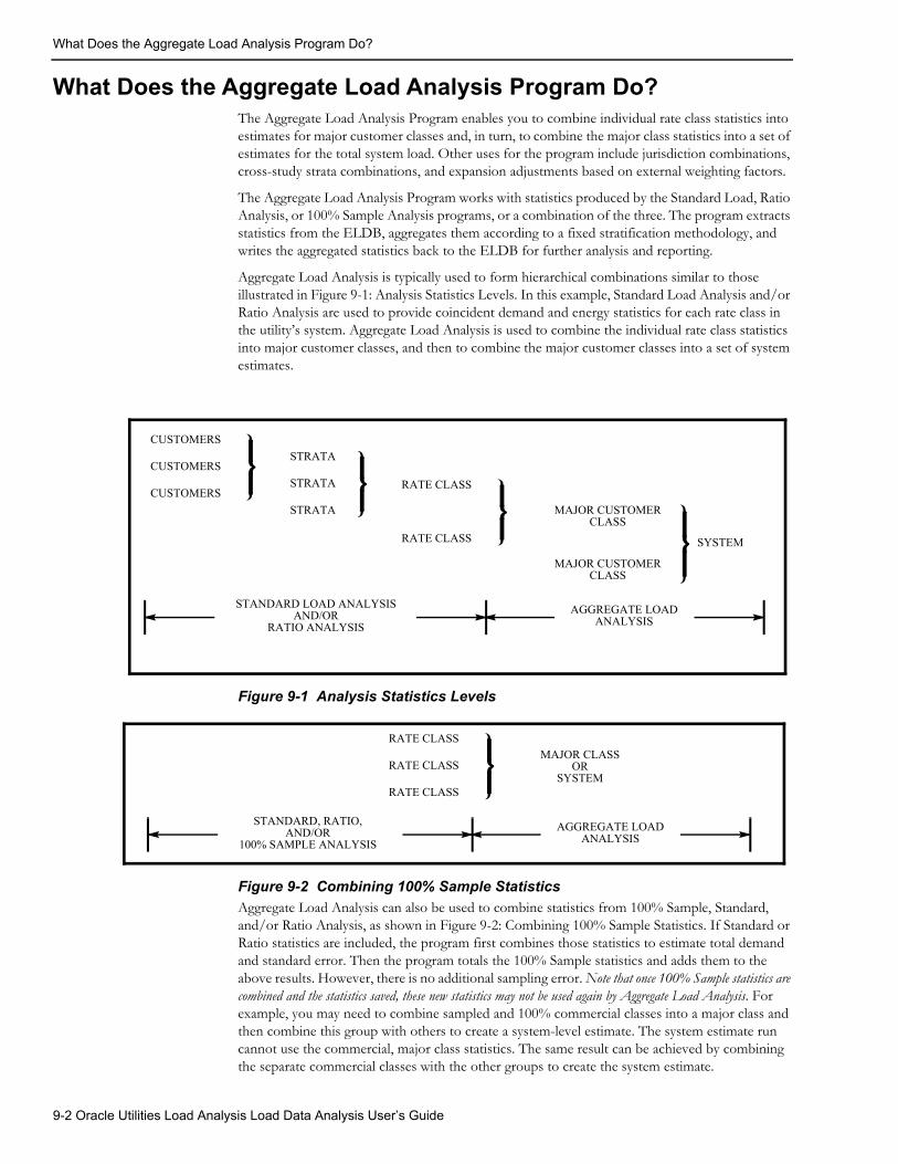
What Does the Aggregate Load Analysis Program Do?
What Does the Aggregate Load Analysis Program Do?The Aggregate Load Analysis Program enables you to combine individual rate class statistics into estimates for major customer classes and, in turn, to combine the major class statistics into a set of estimates for the total system load. Other uses for the program include jurisdiction combinations, cross-study strata combinations, and expansion adjustments based on external weighting factors.
The Aggregate Load Analysis Program works with statistics produced by the Standard Load, Ratio Analysis, or 100% Sample Analysis programs, or a combination of the three. The program extracts statistics from the ELDB, aggregates them according to a fixed stratification methodology, and writes the aggregated statistics back to the ELDB for further analysis and reporting.
Aggregate Load Analysis is typically used to form hierarchical combinations similar to those illustrated in Figure 9-1: Analysis Statistics Levels. In this example, Standard Load Analysis and/or Ratio Analysis are used to provide coincident demand and energy statistics for each rate class in the utility’s system. Aggregate Load Analysis is used to combine the individual rate class statistics into major customer classes, and then to combine the major customer classes into a set of system estimates.
Figure 9-1 Analysis Statistics Levels
Figure 9-2 Combining 100% Sample StatisticsAggregate Load Analysis can also be used to combine statistics from 100% Sample, Standard, and/or Ratio Analysis, as shown in Figure 9-2: Combining 100% Sample Statistics. If Standard or Ratio statistics are included, the program first combines those statistics to estimate total demand and standard error. Then the program totals the 100% Sample statistics and adds them to the above results. However, there is no additional sampling error. Note that once 100% Sample statistics are combined and the statistics saved, these new statistics may not be used again by Aggregate Load Analysis. For example, you may need to combine sampled and 100% commercial classes into a major class and then combine this group with others to create a system-level estimate. The system estimate run cannot use the commercial, major class statistics. The same result can be achieved by combining the separate commercial classes with the other groups to create the system estimate.
CUSTOMERS
CUSTOMERS
CUSTOMERS
STRATA
STRATA
STRATA
RATE CLASS
RATE CLASS
MAJOR CUSTOMERCLASS
MAJOR CUSTOMERCLASS
SYSTEM
AGGREGATE LOAD ANALYSIS
STANDARD LOAD ANALYSISAND/OR
RATIO ANALYSIS
AGGREGATE LOAD ANALYSIS
STANDARD, RATIO,AND/OR
100% SAMPLE ANALYSIS
RATE CLASS
RATE CLASS
MAJOR CLASSOR
SYSTEMRATE CLASS
9-2 Oracle Utilities Load Analysis Load Data Analysis User’s Guide
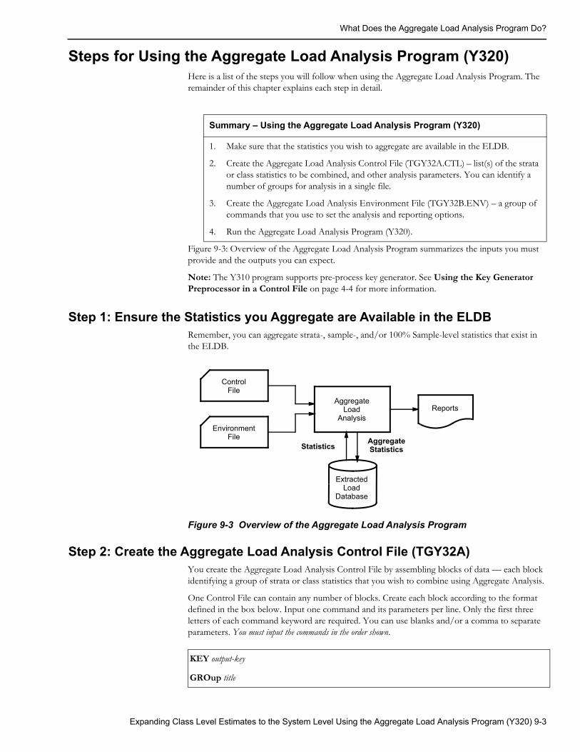
What Does the Aggregate Load Analysis Program Do?
Steps for Using the Aggregate Load Analysis Program (Y320)Here is a list of the steps you will follow when using the Aggregate Load Analysis Program. The remainder of this chapter explains each step in detail.
Figure 9-3: Overview of the Aggregate Load Analysis Program summarizes the inputs you must provide and the outputs you can expect.
Note: The Y310 program supports pre-process key generator. See Using the Key Generator Preprocessor in a Control File on page 4-4 for more information.
Step 1: Ensure the Statistics you Aggregate are Available in the ELDBRemember, you can aggregate strata-, sample-, and/or 100% Sample-level statistics that exist in the ELDB.
Figure 9-3 Overview of the Aggregate Load Analysis Program
Step 2: Create the Aggregate Load Analysis Control File (TGY32A)You create the Aggregate Load Analysis Control File by assembling blocks of data — each block identifying a group of strata or class statistics that you wish to combine using Aggregate Analysis.
One Control File can contain any number of blocks. Create each block according to the format defined in the box below. Input one command and its parameters per line. Only the first three letters of each command keyword are required. You can use blanks and/or a comma to separate parameters. You must input the commands in the order shown.
Summary – Using the Aggregate Load Analysis Program (Y320)
1. Make sure that the statistics you wish to aggregate are available in the ELDB.
2. Create the Aggregate Load Analysis Control File (TGY32A.CTL) – list(s) of the strata or class statistics to be combined, and other analysis parameters. You can identify a number of groups for analysis in a single file.
3. Create the Aggregate Load Analysis Environment File (TGY32B.ENV) – a group of commands that you use to set the analysis and reporting options.
4. Run the Aggregate Load Analysis Program (Y320).
EnvironmentFile
ControlFile
AggregateLoad
AnalysisReports
ExtractedLoad
Database
AggregateStatisticsStatistics
KEY output-key
GROup title
Expanding Class Level Estimates to the System Level Using the Aggregate Load Analysis Program (Y320) 9-3

What Does the Aggregate Load Analysis Program Do?
• Key — This code will become the prefix in the statistics name that Oracle Utilities Load Analysis will assign to the new ELDB statistics. (See Statistics Identifiers on page 3-8).
• You can use up to 40 characters. A combination of characters (A - Z) and digits (0 - 9) may be used, but special characters (anything that is not a letter or number) are not allowed. The identifier must start with an alphabetic character. The default key is "STAR".
• Group — Use the Group Command to designate a title that will appear at the top of each analysis report for the block. The maximum length allowed is 76 characters per title. If you supply two Group commands, the titles will appear on two successive title lines in the sequence given. If you omit the command, no group title will appear.
• Combine — Input one Combine Command for each set of class or strata statistics you want included in a group analysis. Note: The Combine Command applies to statistics from a previous Standard, Ratio, or Aggregate Load Analysis run. Statistics from a 100% Sample Analysis run are not accepted by this command (use 100% instead). Each block must contain at least two Combine and/or 100% commands in any combination (e.g., two of either type or one of each), and all commands in the block must be for compatible statistics. (That is, the statistics to be combined must all have been created over the same date range and using the same Time-Of-Use and Holiday File.) Up to 99 Combine and/or 100% commands may be specified in a block. For a Combine Command, you must supply the following parameters:
component-key — Input the statistics name prefix for the statistics group to be aggregated. Note: A component key is usually a 4-character prefix (e.g., ‘STAR’) and the parameter “strata” (supplied later in the command) is usually ‘0’ (zero); this type of component/strata combination indicates that sample-level statistics are to be used as input. However, if strata-level statistics from Standard Load or Ratio Analysis are desired as input, the “component-key” and “strata” parameters may appear as follows:
If less than 10 strata were used in the Standard Load Analysis or Ratio Analysi run, “component-key” must be specified as a 4- to 6-character code and “strata” must be an integer between 1 and 9, inclusive, e.g., ‘STAR, 2’. If 10 or more strata were used in the Standard Load Analysis or Ratio Analysis run, the “component-key” must be specified as a 7- to 9-character code and “strata” must be 0 (zero); e.g., ‘STAR-02,0’.
type — Indicate the statistics’ type (determined by the analysis methodology used to produce them). Select from these four options:
RATio — non-stratified ratio
COMbined – stratified combined ratio
SEParate — stratified separate ratio
STAndard — standard mean-per-unit or aggregate.
Any one of these four types can be specified. However, for Aggregate Analysis to work properly, the two or more analyses combined must be compatible. That is, they should all be stratified analyses with the same number of strata, or all non-stratified analyses. If type is omitted, the type option defaults to “STANDARD”.
strata — Input a “0”, unless you are combining strata-level statistics from a Standard Load or Ratio Analysis. In that case, enter the appropriate number. (Note: If there are 10
GROup title
COMbine component-key1 [,type] [,strata1 | ,0 [,weight1 | ,0.0 [,factor1 | ,1.0] ] ]
COMbine component-key2 [,type] [,strata2 | ,0 [,weight2 | ,0.0 [,factor2 | ,1.0] ] ]
COMbine component-keyN [,type] [,strataN | ,0 [,weightN | ,0.0 [,factorN | ,1.0] ] ]
100%—component-key N+1 [,factorN+1 | 1.0]
END
9-4 Oracle Utilities Load Analysis Load Data Analysis User’s Guide
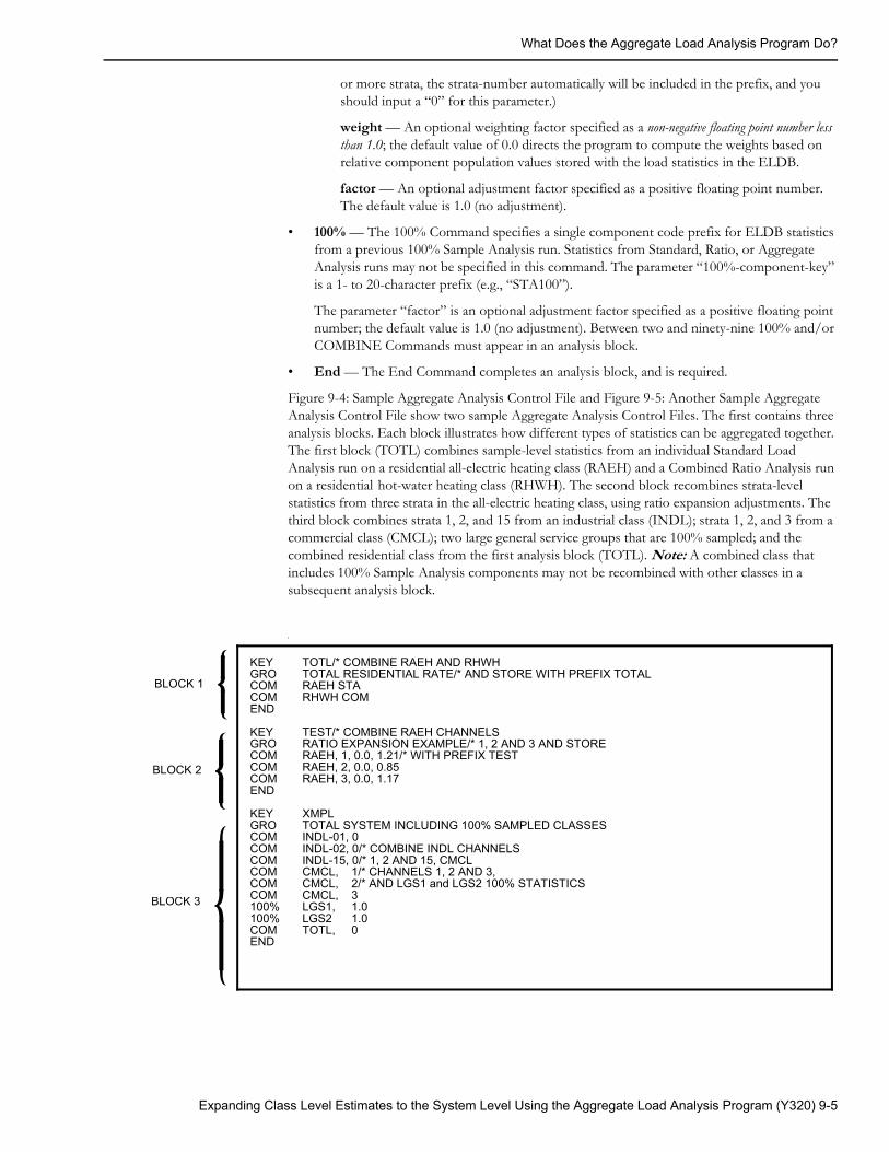
What Does the Aggregate Load Analysis Program Do?
or more strata, the strata-number automatically will be included in the prefix, and you should input a “0” for this parameter.)
weight — An optional weighting factor specified as a non-negative floating point number less than 1.0; the default value of 0.0 directs the program to compute the weights based on relative component population values stored with the load statistics in the ELDB.
factor — An optional adjustment factor specified as a positive floating point number. The default value is 1.0 (no adjustment).
• 100% — The 100% Command specifies a single component code prefix for ELDB statistics from a previous 100% Sample Analysis run. Statistics from Standard, Ratio, or Aggregate Analysis runs may not be specified in this command. The parameter “100%-component-key” is a 1- to 20-character prefix (e.g., “STA100”).
The parameter “factor” is an optional adjustment factor specified as a positive floating point number; the default value is 1.0 (no adjustment). Between two and ninety-nine 100% and/or COMBINE Commands must appear in an analysis block.
• End — The End Command completes an analysis block, and is required.
Figure 9-4: Sample Aggregate Analysis Control File and Figure 9-5: Another Sample Aggregate Analysis Control File show two sample Aggregate Analysis Control Files. The first contains three analysis blocks. Each block illustrates how different types of statistics can be aggregated together. The first block (TOTL) combines sample-level statistics from an individual Standard Load Analysis run on a residential all-electric heating class (RAEH) and a Combined Ratio Analysis run on a residential hot-water heating class (RHWH). The second block recombines strata-level statistics from three strata in the all-electric heating class, using ratio expansion adjustments. The third block combines strata 1, 2, and 15 from an industrial class (INDL); strata 1, 2, and 3 from a commercial class (CMCL); two large general service groups that are 100% sampled; and the combined residential class from the first analysis block (TOTL). Note: A combined class that includes 100% Sample Analysis components may not be recombined with other classes in a subsequent analysis block.
f
KEY TOTL/* COMBINE RAEH AND RHWHGRO TOTAL RESIDENTIAL RATE/* AND STORE WITH PREFIX TOTALCOM RAEH STACOM RHWH COMEND
KEY TEST/* COMBINE RAEH CHANNELS GRO RATIO EXPANSION EXAMPLE/* 1, 2 AND 3 AND STORECOM RAEH, 1, 0.0, 1.21/* WITH PREFIX TESTCOM RAEH, 2, 0.0, 0.85COM RAEH, 3, 0.0, 1.17END
KEY XMPLGRO TOTAL SYSTEM INCLUDING 100% SAMPLED CLASSESCOM INDL-01, 0COM INDL-02, 0/* COMBINE INDL CHANNELSCOM INDL-15, 0/* 1, 2 AND 15, CMCLCOM CMCL, 1/* CHANNELS 1, 2 AND 3,COM CMCL, 2/* AND LGS1 and LGS2 100% STATISTICSCOM CMCL, 3100% LGS1, 1.0100% LGS2 1.0COM TOTL, 0END
BLOCK 1
BLOCK 2
BLOCK 3
Expanding Class Level Estimates to the System Level Using the Aggregate Load Analysis Program (Y320) 9-5
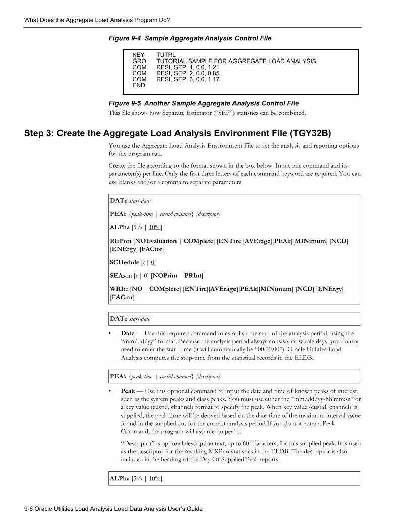
What Does the Aggregate Load Analysis Program Do?
Figure 9-4 Sample Aggregate Analysis Control File
Figure 9-5 Another Sample Aggregate Analysis Control FileThis file shows how Separate Estimator (“SEP”) statistics can be combined.
Step 3: Create the Aggregate Load Analysis Environment File (TGY32B)You use the Aggregate Load Analysis Environment File to set the analysis and reporting options for the program run.
Create the file according to the format shown in the box below. Input one command and its parameter(s) per line. Only the first three letters of each command keyword are required. You can use blanks and/or a comma to separate parameters.
• Date — Use this required command to establish the start of the analysis period, using the “mm/dd/yy” format. Because the analysis period always consists of whole days, you do not need to enter the start-time (it will automatically be “00:00:00”). Oracle Utilities Load Analysis computes the stop-time from the statistical records in the ELDB.
• Peak — Use this optional command to input the date and time of known peaks of interest, such as the system peaks and class peaks. You must use either the “mm/dd/yy-hh:mm:ss” or a key value (custid, channel) format to specify the peak. When key value (custid, channel) is supplied, the peak-time will be derived based on the date-time of the maximum interval value found in the supplied cut for the current analysis period.If you do not enter a Peak Command, the program will assume no peaks.
“Descriptor” is optional description text, up to 60 characters, for this supplied peak. It is used as the descriptor for the resulting MXPnn statistics in the ELDB. The descriptor is also included in the heading of the Day Of Supplied Peak reports.
KEY TUTRLGRO TUTORIAL SAMPLE FOR AGGREGATE LOAD ANALYSISCOM RESI, SEP, 1, 0.0, 1.21COM RESI, SEP, 2, 0.0, 0.85COM RESI, SEP, 3, 0.0, 1.17END
DATe start-date
PEAk {peak-time | custid channel} [descriptor]
ALPha [5% | 10%]
REPort [NOEvaluation | COMplete] [ENTire][AVErage][PEAk][MINimum] [NCD] [ENErgy] [FACtor]
SCHedule [t | 0]
SEAson [s | 0] [NOPrint | PRInt]
WRIte [NO | COMplete] [ENTire][AVErage][PEAk][MINimum] [NCD] [ENErgy] [FACtor]
DATe start-date
PEAk {peak-time | custid channel} [descriptor]
ALPha [5% | 10%]
9-6 Oracle Utilities Load Analysis Load Data Analysis User’s Guide
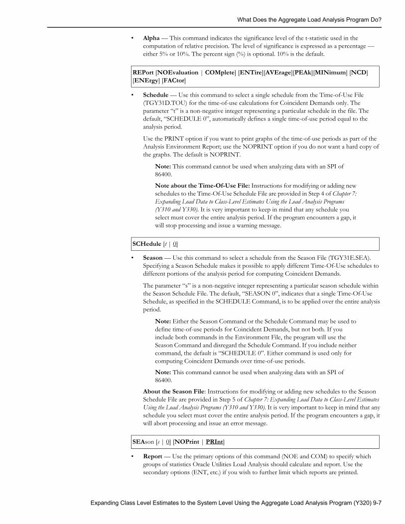
What Does the Aggregate Load Analysis Program Do?
• Alpha — This command indicates the significance level of the t-statistic used in the computation of relative precision. The level of significance is expressed as a percentage — either 5% or 10%. The percent sign (%) is optional. 10% is the default.
• Schedule — Use this command to select a single schedule from the Time-of-Use File (TGY31D.TOU) for the time-of-use calculations for Coincident Demands only. The parameter “t” is a non-negative integer representing a particular schedule in the file. The default, “SCHEDULE 0”, automatically defines a single time-of-use period equal to the analysis period.
Use the PRINT option if you want to print graphs of the time-of-use periods as part of the Analysis Environment Report; use the NOPRINT option if you do not want a hard copy of the graphs. The default is NOPRINT.
Note: This command cannot be used when analyzing data with an SPI of 86400.
Note about the Time-Of-Use File: Instructions for modifying or adding new schedules to the Time-Of-Use Schedule File are provided in Step 4 of Chapter 7: Expanding Load Data to Class-Level Estimates Using the Load Analysis Programs (Y310 and Y330). It is very important to keep in mind that any schedule you select must cover the entire analysis period. If the program encounters a gap, it will stop processing and issue a warning message.
• Season — Use this command to select a schedule from the Season File (TGY31E.SEA). Specifying a Season Schedule makes it possible to apply different Time-Of-Use schedules to different portions of the analysis period for computing Coincident Demands.
The parameter “s” is a non-negative integer representing a particular season schedule within the Season Schedule File. The default, “SEASON 0”, indicates that a single Time-Of-Use Schedule, as specified in the SCHEDULE Command, is to be applied over the entire analysis period.
Note: Either the Season Command or the Schedule Command may be used to define time-of-use periods for Coincident Demands, but not both. If you include both commands in the Environment File, the program will use the Season Command and disregard the Schedule Command. If you include neither command, the default is “SCHEDULE 0”. Either command is used only for computing Coincident Demands over time-of-use periods.
Note: This command cannot be used when analyzing data with an SPI of 86400.
About the Season File: Instructions for modifying or adding new schedules to the Season Schedule File are provided in Step 5 of Chapter 7: Expanding Load Data to Class-Level Estimates Using the Load Analysis Programs (Y310 and Y330). It is very important to keep in mind that any schedule you select must cover the entire analysis period. If the program encounters a gap, it will abort processing and issue an error message.
• Report — Use the primary options of this command (NOE and COM) to specify which groups of statistics Oracle Utilities Load Analysis should calculate and report. Use the secondary options (ENT, etc.) if you wish to further limit which reports are printed.
REPort [NOEvaluation | COMplete] [ENTire][AVErage][PEAk][MINimum] [NCD] [ENErgy] [FACtor]
SCHedule [t | 0]
SEAson [s | 0] [NOPrint | PRInt]
Expanding Class Level Estimates to the System Level Using the Aggregate Load Analysis Program (Y320) 9-7
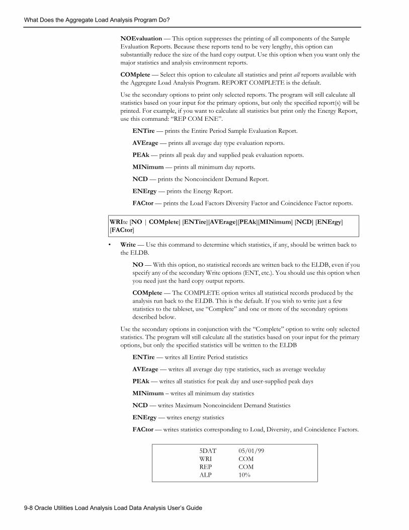
What Does the Aggregate Load Analysis Program Do?
NOEvaluation — This option suppresses the printing of all components of the Sample Evaluation Reports. Because these reports tend to be very lengthy, this option can substantially reduce the size of the hard copy output. Use this option when you want only the major statistics and analysis environment reports.
COMplete — Select this option to calculate all statistics and print all reports available with the Aggregate Load Analysis Program. REPORT COMPLETE is the default.
Use the secondary options to print only selected reports. The program will still calculate all statistics based on your input for the primary options, but only the specified report(s) will be printed. For example, if you want to calculate all statistics but print only the Energy Report, use this command: “REP COM ENE”.
ENTire — prints the Entire Period Sample Evaluation Report.
AVErage — prints all average day type evaluation reports.
PEAk — prints all peak day and supplied peak evaluation reports.
MINimum — prints all minimum day reports.
NCD — prints the Noncoincident Demand Report.
ENErgy — prints the Energy Report.
FACtor — prints the Load Factors Diversity Factor and Coincidence Factor reports.
• Write — Use this command to determine which statistics, if any, should be written back to the ELDB.
NO — With this option, no statistical records are written back to the ELDB, even if you specify any of the secondary Write options (ENT, etc.). You should use this option when you need just the hard copy output reports.
COMplete — The COMPLETE option writes all statistical records produced by the analysis run back to the ELDB. This is the default. If you wish to write just a few statistics to the tableset, use “Complete” and one or more of the secondary options described below.
Use the secondary options in conjunction with the “Complete” option to write only selected statistics. The program will still calculate all the statistics based on your input for the primary options, but only the specified statistics will be written to the ELDB
ENTire — writes all Entire Period statistics
AVErage — writes all average day type statistics, such as average weekday
PEAk — writes all statistics for peak day and user-supplied peak days
MINimum – writes all minimum day statistics
NCD — writes Maximum Noncoincident Demand Statistics
ENErgy — writes energy statistics
FACtor — writes statistics corresponding to Load, Diversity, and Coincidence Factors.
WRIte [NO | COMplete] [ENTire][AVErage][PEAk][MINimum] [NCD] [ENErgy] [FACtor]
5DAT WRI REP ALP
05/01/99COMCOM10%
9-8 Oracle Utilities Load Analysis Load Data Analysis User’s Guide

What Does the Aggregate Load Analysis Program Do?
Figure 9-6 Sample Aggregate Analysis Environment File
Step 4: Run the Aggregate Load Analysis Program (Y320)Once you have created the Control and Environment files, you are ready to run the Analysis Program. Use Y320.
Aggregate Analysis ProcessingThe Aggregate Load Analysis Program initially examines the Environment File for errors and reports fatal errors with a diagnostic message. Those environment parameters that are not specified are assigned default values. The contents of the Environment File apply to all subsequent analyses.
The program then processes analysis blocks in the Control File. A block is defined by a KEY Command, an optional GROUP Command, between 2 and 99 COMBINE and/or 100% commands, and a single END Command. Illegal commands and errors are noted with a diagnostic message; if errors are found, the block is discarded and processing resumes with the next block.
For each valid analysis block, the program extracts certain statistical records in the ELDB for the indicated components, aggregates the statistics using the methodology presented in Appendix B: Analysis Equations, and writes the aggregated statistics back to the ELDB using the key specified in the KEY Command.
The Aggregate Load Analysis Program will attempt to calculate the following load statistics:
• Average day demands
• Average day demands, excluding holiday
• Average weekday demands
• Average weekday demands, excluding holiday
• Coincident demands over the entire period
• Average weekend demands
• Average weekend demands, excluding holidays
• Average day-of-the-week demands
• Average weekday holiday demands
• Average weekend holiday demands
• Average weekend including weekday holiday demands
• Average User-Specified Day (if available)
• Day of supplied peak demands
• Total energy, by time-of-use
• Non-coincident demand, by time-of-use
• Load factor for non-coincident demand
• Load factors for maximum coincident demand and for demand at time of supplied peaks
• Diversity factors for maximum coincident demand and for demand at time of supplied peaks
• Coincidence factors for maximum coincident demand and for demand at time of supplied peaks.
The steps required to develop the above load statistics depend upon the mode of analysis. The Sample Only mode occurs when only Combine commands are used in the command block and all
Expanding Class Level Estimates to the System Level Using the Aggregate Load Analysis Program (Y320) 9-9
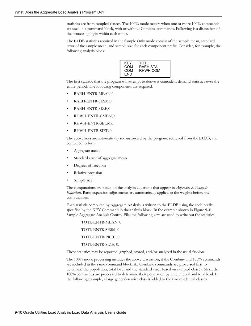
What Does the Aggregate Load Analysis Program Do?
statistics are from sampled classes. The 100% mode occurs when one or more 100% commands are used in a command block, with or without Combine commands. Following is a discussion of the processing logic within each mode.
The ELDB statistics required in the Sample Only mode consist of the sample mean, standard error of the sample mean, and sample size for each component prefix. Consider, for example, the following analysis block:
The first statistic that the program will attempt to derive is coincident demand statistics over the entire period. The following components are required.
• RAEH-ENTR-MEAN,0
• RAEH-ENTR-SESM,0
• RAEH-ENTR-SIZE,0
• RHWH-ENTR-CMEN,0
• RHWH-ENTR-SECM,0
• RHWH-ENTR-SIZE,0.
The above keys are automatically reconstructed by the program, retrieved from the ELDB, and combined to form:
• Aggregate mean
• Standard error of aggregate mean
• Degrees of freedom
• Relative precision
• Sample size.
The computations are based on the analysis equations that appear in Appendix B: Analysis Equations. Ratio expansion adjustments are automatically applied to the weights before the computations.
Each statistic computed by Aggregate Analysis is written to the ELDB using the code prefix specified by the KEY Command in the analysis block. In the example shown in Figure 9-4: Sample Aggregate Analysis Control File, the following keys are used to write out the statistics.
TOTL-ENTR-MEAN, 0
TOTL-ENTR-SESM, 0
TOTL-ENTR-PREC, 0
TOTL-ENTR-SIZE, 0.
These statistics may be reported, graphed, stored, and/or analyzed in the usual fashion.
The 100% mode processing includes the above discussion, if the Combine and 100% commands are included in the same command block. All Combine commands are processed first to determine the population, total load, and the standard error based on sampled classes. Next, the 100% commands are processed to determine their population by time interval and total load. In the following example, a large general-service class is added to the two residential classes:
KEY TOTLCOM RAEH STACOM RHWH COMEND
9-10 Oracle Utilities Load Analysis Load Data Analysis User’s Guide
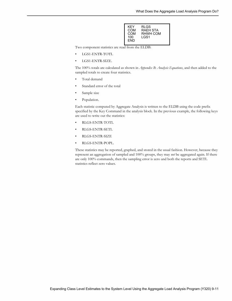
What Does the Aggregate Load Analysis Program Do?
Two component statistics are read from the ELDB:
• LGS1-ENTR-TOTL
• LGS1-ENTR-SIZE.
The 100% totals are calculated as shown in Appendix B: Analysis Equations, and then added to the sampled totals to create four statistics.
• Total demand
• Standard error of the total
• Sample size
• Population.
Each statistic computed by Aggregate Analysis is written to the ELDB using the code prefix specified by the Key Command in the analysis block. In the previous example, the following keys are used to write out the statistics:
• RLGS-ENTR-TOTL
• RLGS-ENTR-SETL
• RLGS-ENTR-SIZE
• RLGS-ENTR-POPL.
These statistics may be reported, graphed, and stored in the usual fashion. However, because they represent an aggregation of sampled and 100% groups, they may not be aggregated again. If there are only 100% commands, then the sampling error is zero and both the reports and SETL statistics reflect zero values.
KEY RLGSCOM RAEH STACOM RHWH COM100 LGS1END
Expanding Class Level Estimates to the System Level Using the Aggregate Load Analysis Program (Y320) 9-11

What Does the Aggregate Load Analysis Program Do?
9-12 Oracle Utilities Load Analysis Load Data Analysis User’s Guide
Chapter 10Estimating Average Peak Load Using the
Coincident Peak Analysis Program (Y340)
In this chapter we will look at the Coincident Peak Analysis Program. This program enables you to calculate the estimate of the mean and corresponding sampling error of up to twelve periods of coincident peak demands for a customer class. Topics covered in this chapter include:
• What Does the Coincident Peak Analysis Program Do?
• Steps for Using the Coincident Peak Analysis Program (Y340)
Estimating Average Peak Load Using the Coincident Peak Analysis Program (Y340) 10-1

What Does the Coincident Peak Analysis Program Do?
What Does the Coincident Peak Analysis Program Do?Coincident peak analysis is a powerful methodology for determining the responsibility of a rate class when allocating costs. Often the allocation of costs to a rate class is done using statistics that reflect just one hour of demand, such as maximum coincident demand at the time of system peak, or maximum non-coincident demand. The problem with these statistics is their concentration on one hour of the year to the exclusion of all others. Coincident peak analysis provides the capability to combine the contributions of special hours into a more representative measure upon which to allocate. The hours included may represent monthly peaks for the year, or a subset of months corresponding to seasonal peaks.
The Oracle Utilities Load Analysis Coincident Peak Analysis Program can be used to calculate the estimate of the mean and corresponding sampling error of up to 12 periods of coincident peak demands for a specified class of customers. (See Figure 10-1: Coincident Peak Analysis.) The estimates may be calculated with either of two techniques: mean-per-unit or combined ratio estimation. Both are sophisticated analysis techniques that yield results at the class and average customer levels. (See the beginning of Chapter 7: Expanding Load Data to Class-Level Estimates Using the Load Analysis Programs (Y310 and Y330) for a discussion of the differences between the mean-per-unit and combined ratio expansion methodologies.) You can even request that the program perform both types of analysis in a single run.
Note: Combined ratio estimation requires accurate billed energy values for the entire customer class population, broken down by analysis sub-period. It is also helpful to have billed energy values for each customer in the sample, by sub-period, but that is not a requirement.
The Coincident Peak Analysis Program offers several additional options, giving you greater control over the analysis — including analysis of stratified or non-stratified samples; the ability to filter interval data by quality; the option to use data from either the ALDB or ELDB, or both; and the capability to adjust for changing strata populations.
The results of the computations are eight output reports: an Environment Report, an Individual Customer Definition Report, a Strata Statistics Matrix Report by strata, a Variance/Covariance Matrix Report, two Coincident Peak reports, an optional Customer Error Report, and an optional Strata Population/Weight Update Report.
10-2 Oracle Utilities Load Analysis Load Data Analysis User’s Guide
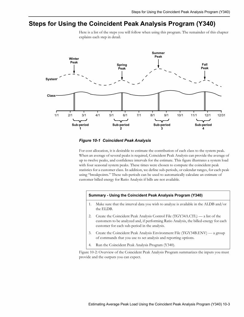
Steps for Using the Coincident Peak Analysis Program (Y340)
Steps for Using the Coincident Peak Analysis Program (Y340)Here is a list of the steps you will follow when using this program. The remainder of this chapter explains each step in detail.
Figure 10-1 Coincident Peak Analysis
For cost allocation, it is desirable to estimate the contribution of each class to the system peak. When an average of several peaks is required, Coincident Peak Analysis can provide the average of up to twelve peaks, and confidence intervals for the estimate. This figure illustrates a system load with four seasonal system peaks. These times were chosen to compute the coincident peak statistics for a customer class. In addition, we define sub-periods, or calendar ranges, for each peak using “breakpoints.” These sub-periods can be used to automatically calculate an estimate of customer billed energy for Ratio Analysis if bills are not available.
Figure 10-2: Overview of the Coincident Peak Analysis Program summarizes the inputs you must provide and the outputs you can expect.
1/1 2/1 3/1 4/1 5/1 6/1 7/1 8/1 9/1 10/1 11/1 12/1 12/31
Sub-period1
Sub-period2
Sub-period3
Sub-period4
Class
System
WinterPeak
SpringPeak
SummerPeak
FallPeak
Summary - Using the Coincident Peak Analysis Program (Y340)
1. Make sure that the interval data you wish to analyze is available in the ALDB and/or the ELDB.
2. Create the Coincident Peak Analysis Control File (TGY34A.CTL) — a list of the customers to be analyzed and, if performing Ratio Analysis, the billed-energy for each customer for each sub-period in the analysis.
3. Create the Coincident Peak Analysis Environment File (TGY34B.ENV) — a group of commands that you use to set analysis and reporting options.
4. Run the Coincident Peak Analysis Program (Y340).
Estimating Average Peak Load Using the Coincident Peak Analysis Program (Y340) 10-3
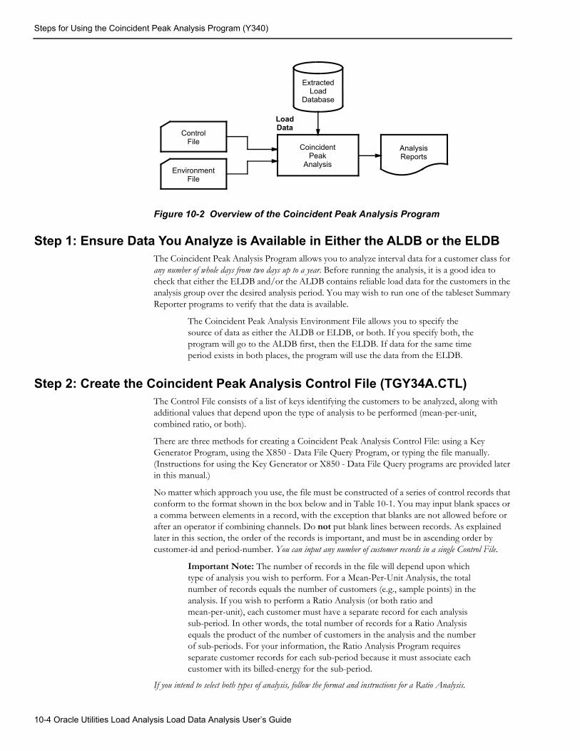
Steps for Using the Coincident Peak Analysis Program (Y340)
Figure 10-2 Overview of the Coincident Peak Analysis Program
Step 1: Ensure Data You Analyze is Available in Either the ALDB or the ELDBThe Coincident Peak Analysis Program allows you to analyze interval data for a customer class for any number of whole days from two days up to a year. Before running the analysis, it is a good idea to check that either the ELDB and/or the ALDB contains reliable load data for the customers in the analysis group over the desired analysis period. You may wish to run one of the tableset Summary Reporter programs to verify that the data is available.
The Coincident Peak Analysis Environment File allows you to specify the source of data as either the ALDB or ELDB, or both. If you specify both, the program will go to the ALDB first, then the ELDB. If data for the same time period exists in both places, the program will use the data from the ELDB.
Step 2: Create the Coincident Peak Analysis Control File (TGY34A.CTL)The Control File consists of a list of keys identifying the customers to be analyzed, along with additional values that depend upon the type of analysis to be performed (mean-per-unit, combined ratio, or both).
There are three methods for creating a Coincident Peak Analysis Control File: using a Key Generator Program, using the X850 - Data File Query Program, or typing the file manually. (Instructions for using the Key Generator or X850 - Data File Query programs are provided later in this manual.)
No matter which approach you use, the file must be constructed of a series of control records that conform to the format shown in the box below and in Table 10-1. You may input blank spaces or a comma between elements in a record, with the exception that blanks are not allowed before or after an operator if combining channels. Do not put blank lines between records. As explained later in this section, the order of the records is important, and must be in ascending order by customer-id and period-number. You can input any number of customer records in a single Control File.
Important Note: The number of records in the file will depend upon which type of analysis you wish to perform. For a Mean-Per-Unit Analysis, the total number of records equals the number of customers (e.g., sample points) in the analysis. If you wish to perform a Ratio Analysis (or both ratio and mean-per-unit), each customer must have a separate record for each analysis sub-period. In other words, the total number of records for a Ratio Analysis equals the product of the number of customers in the analysis and the number of sub-periods. For your information, the Ratio Analysis Program requires separate customer records for each sub-period because it must associate each customer with its billed-energy for the sub-period.
If you intend to select both types of analysis, follow the format and instructions for a Ratio Analysis.
CoincidentPeak
Analysis
AnalysisReports
ExtractedLoad
Database
LoadData
ControlFile
EnvironmentFile
10-4 Oracle Utilities Load Analysis Load Data Analysis User’s Guide

Steps for Using the Coincident Peak Analysis Program (Y340)
Control File Record Format for Mean-Per-Unit Analysis:
Control File Record Format For Combined Ratio Analysis, or Both:
• customer-id — enter the Oracle Utilities Load Analysis customer-id. Required.
• chan1, chan2...chanx — enter the channel-number or a combination of channels for that customer-id. At least one channel-number per record is required.
A combination consists of two or more channels added or subtracted to represent the total customer load. For example, 1+2-7 might be used to represent the sum of channels 1 and 2 minus channel 7, a co-generation unit. Do not add blanks before or after an operator. Note: The data is combined strictly for the analysis; no new records are created.
When deciding whether or not to combine channel-numbers, it is important to remember that each record in the Control File represents one sample point in the analysis. If you are analyzing end-uses, it would be appropriate to keep channel-numbers separate. If you are analyzing total premise loads, you would typically combine the channel-numbers for a large customer into a single record. (Note: If you want to combine multiple customer-ids into a single sample point, you cannot do that in the Control File. You must instead use the Load Data Transformation Program, Y620, before analysis.)
• strata-number — enter the stratum number to which the customer belongs. Required for either type of analysis.
• customer-billed-energy — for Ratio Analysis — enter the amount of energy for which the customer was billed for the analysis sub-period. (The particular analysis sub-period is identified with the next parameter in the command, as described below.) The billed-energy value should come from “billing.” Enter it as a positive floating point number.
If you cannot provide accurate billed energy values for the customers in the analysis, you can have the program calculate the values from the interval data. To do this, you must provide two pieces of information in the Environment File: 1) select the BILLING NO option; and 2) identify the date range of each analysis sub-period using “breakpoints” (explained later in this chapter). Also, be sure to provide a zero or other value in the Control File record as a place-holder (it will not be used in the calculations).
Alternatively, if you are missing just a few values, you can direct the program to drop customers for just specific sub-periods. That is, if a customer has an unacceptable or missing billed-energy value for a particular sub-period, you may insert a negative integer for billed-energy in the Control File to indicate the situation. Doing this will cause the customer’s data contribution to be dropped from the analysis for that sub-period only.
If you are performing a Ratio Analysis, all Control File records must include a billed-energy value (even if it is just a place-holder) and an associated period number. If the program finds any missing values, they will be considered a fatal error and the program will terminate processing.
• period-number — required for Ratio Analysis — a positive integer that identifies a sub-period in the analysis. The customer billed-energy value you supplied in the previous parameter in the record must belong to this sub-period.
If you do not supply a period number for each record in a Ratio Analysis, the program will abort processing.
To obtain a better understanding of the organization of a typical Control File, consider the following two examples. The first example (Figure 10-3: Sample Control File for Stratified,
customer-id chan1 [{±}chan2 [{±}chan3...[{±}chann ] ] ] [stratum-number]
customer-id chan1 [{±}chan2 [{±}chan3...[{±}chann ] ] ][stratum-number] [customer-billed-energy][period-number]
Estimating Average Peak Load Using the Coincident Peak Analysis Program (Y340) 10-5
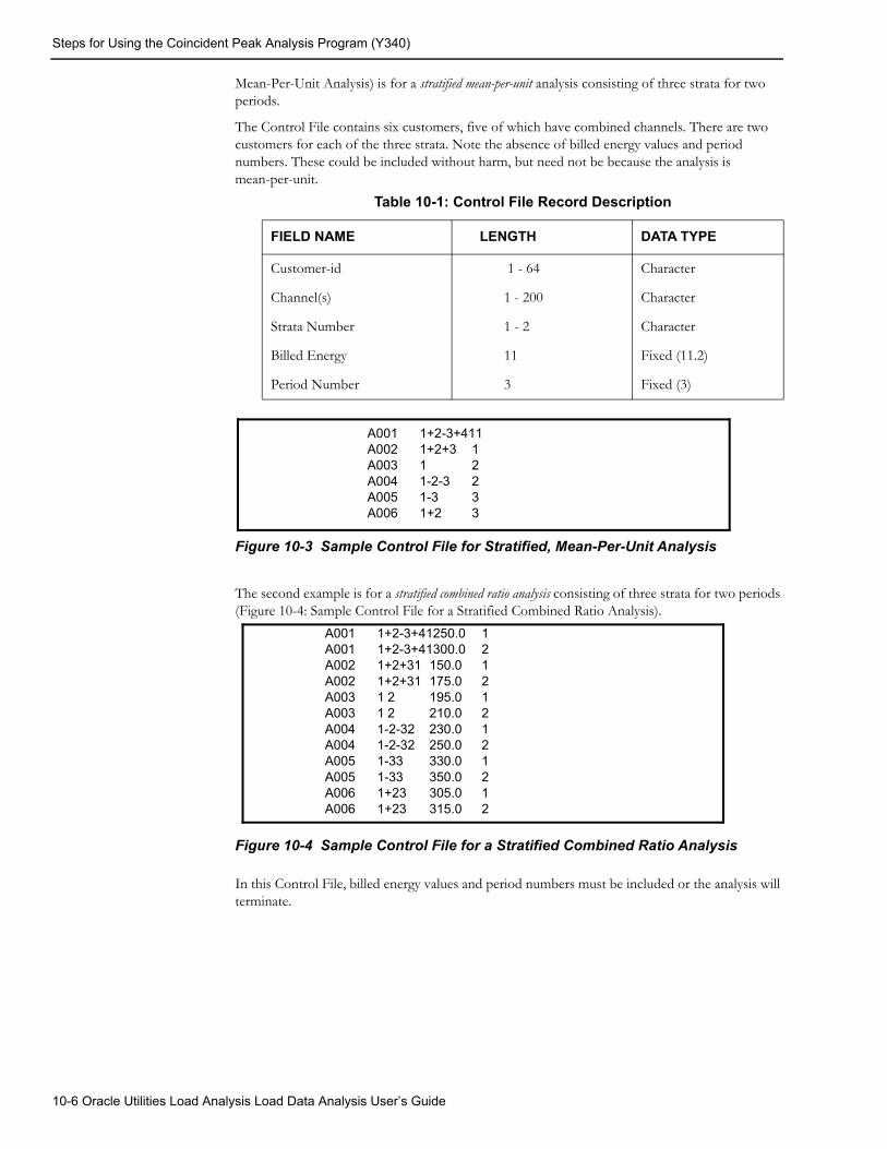
Steps for Using the Coincident Peak Analysis Program (Y340)
Mean-Per-Unit Analysis) is for a stratified mean-per-unit analysis consisting of three strata for two periods.
The Control File contains six customers, five of which have combined channels. There are two customers for each of the three strata. Note the absence of billed energy values and period numbers. These could be included without harm, but need not be because the analysis is mean-per-unit.
Figure 10-3 Sample Control File for Stratified, Mean-Per-Unit Analysis
The second example is for a stratified combined ratio analysis consisting of three strata for two periods (Figure 10-4: Sample Control File for a Stratified Combined Ratio Analysis).
Figure 10-4 Sample Control File for a Stratified Combined Ratio Analysis
In this Control File, billed energy values and period numbers must be included or the analysis will terminate.
Table 10-1: Control File Record Description
FIELD NAME LENGTH DATA TYPE
Customer-id 1 - 64 Character
Channel(s) 1 - 200 Character
Strata Number 1 - 2 Character
Billed Energy 11 Fixed (11.2)
Period Number 3 Fixed (3)
A001 1+2-3+411A002 1+2+3 1A003 1 2A004 1-2-3 2A005 1-3 3A006 1+2 3
A001 1+2-3+41250.0 1A001 1+2-3+41300.0 2A002 1+2+31 150.0 1A002 1+2+31 175.0 2A003 1 2 195.0 1A003 1 2 210.0 2A004 1-2-32 230.0 1A004 1-2-32 250.0 2A005 1-33 330.0 1A005 1-33 350.0 2A006 1+23 305.0 1A006 1+23 315.0 2
10-6 Oracle Utilities Load Analysis Load Data Analysis User’s Guide
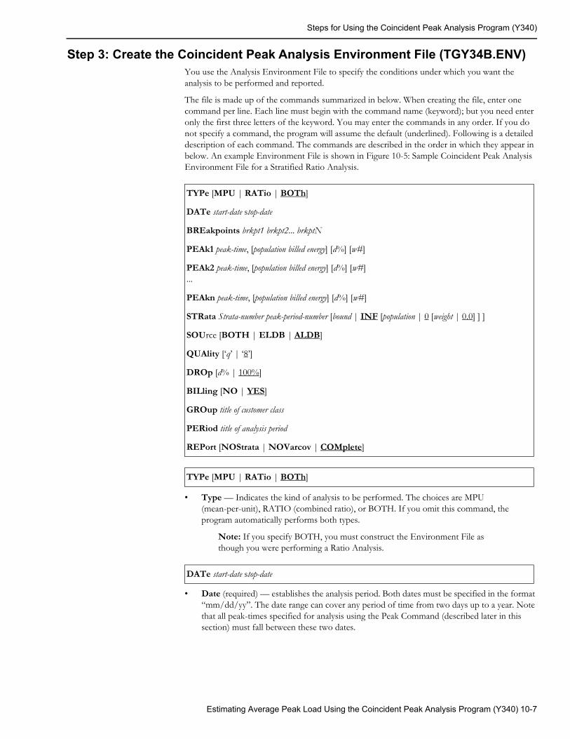
Steps for Using the Coincident Peak Analysis Program (Y340)
Step 3: Create the Coincident Peak Analysis Environment File (TGY34B.ENV)You use the Analysis Environment File to specify the conditions under which you want the analysis to be performed and reported.
The file is made up of the commands summarized in below. When creating the file, enter one command per line. Each line must begin with the command name (keyword); but you need enter only the first three letters of the keyword. You may enter the commands in any order. If you do not specify a command, the program will assume the default (underlined). Following is a detailed description of each command. The commands are described in the order in which they appear in below. An example Environment File is shown in Figure 10-5: Sample Coincident Peak Analysis Environment File for a Stratified Ratio Analysis.
• Type — Indicates the kind of analysis to be performed. The choices are MPU (mean-per-unit), RATIO (combined ratio), or BOTH. If you omit this command, the program automatically performs both types.
Note: If you specify BOTH, you must construct the Environment File as though you were performing a Ratio Analysis.
• Date (required) — establishes the analysis period. Both dates must be specified in the format “mm/dd/yy”. The date range can cover any period of time from two days up to a year. Note that all peak-times specified for analysis using the Peak Command (described later in this section) must fall between these two dates.
TYPe [MPU | RATio | BOTh]
DATe start-date stop-date
BREakpoints brkpt1 brkpt2... brkptN
PEAk1 peak-time, [population billed energy] [d%] [w#]
PEAk2 peak-time, [population billed energy] [d%] [w#]...
PEAkn peak-time, [population billed energy] [d%] [w#]
STRata Strata-number peak-period-number [bound | INF [population | 0 [weight | 0.0] ] ]
SOUrce [BOTH | ELDB | ALDB]
QUAlity [‘q’ | ‘8’]
DROp [d% | 100%]
BILling [NO | YES]
GROup title of customer class
PERiod title of analysis period
REPort [NOStrata | NOVarcov | COMplete]
TYPe [MPU | RATio | BOTh]
DATe start-date stop-date
Estimating Average Peak Load Using the Coincident Peak Analysis Program (Y340) 10-7
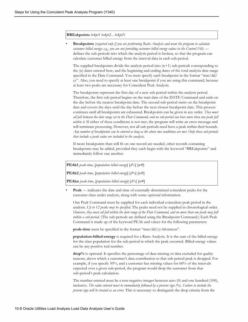
Steps for Using the Coincident Peak Analysis Program (Y340)
• Breakpoints (required only if you are performing Ratio Analysis and want the program to calculate customer billed energy; e.g., you are not providing customer billed energy values in the Control File) — defines the sub-periods into which the analysis period is broken, so that the program can calculate customer billed energy from the interval data in each sub-period.
The supplied breakpoints divide the analysis period into (n+1) sub-periods corresponding to the (n) dates entered here, and the beginning and ending dates of the total analysis date range specified in the Date Command. You must specify each breakpoint in the format “mm/dd/yy”. Also, you need to specify at least one breakpoint if you are using this command, because at least two peaks are necessary for Coincident Peak Analysis.
The breakpoints represent the first day of a new sub-period within the analysis period. Therefore, the first sub-period begins on the start-date of the DATE Command and ends on the day before the nearest breakpoint date. The second sub-period starts on the breakpoint date and covers the days until the day before the next closest breakpoint date. This process continues until all breakpoints are exhausted. Breakpoints can be given in any order. They must all fall between the date range set in the Date Command, and no sub-period can have more than one peak fall within it. If either of these conditions is not met, the program will write an error message and will terminate processing. However, not all sub-periods need have a peak within their bounds. Any number of breakpoints can be entered as long as the above two conditions are met. Only those sub-periods that include a peak value are included in the analysis.
If more breakpoints than will fit on one record are needed, other records containing breakpoints may be added, provided they each begin with the keyword “BREakpoints” and immediately follow one another.
• Peak — indicates the date and time of externally determined coincident peaks for the customer class under analysis, along with some optional information.
One Peak Command must be supplied for each individual coincident peak period in the analysis. Up to 12 peaks may be specified. The peaks need not be supplied in chronological order. However, they must all fall within the date range of the Date Command, and no more than one peak may fall within a sub-period. (The sub-periods are defined using the Breakpoint Command.) Each Peak Command is made up of the keyword PEAk and values for the following parameters:
peak-time must be specified in the format “mm/dd/yy-hh:mm:ss”.
population-billed-energy is required for a Ratio Analysis. It is the sum of the billed-energy for the class population for the sub-period in which the peak occurred. Billed-energy values can be any positive real number.
drop% is optional. It specifies the percentage of data missing or data excluded for quality reasons, above which a customer’s data contribution to that sub-period peak is dropped. For example, if you specify 50%, and a customer has missing values for 60% of the intervals expected over a given sub-period, the program would drop the customer from that sub-period’s peak calculation.
The number entered must be a non-negative integer between zero (0) and one hundred (100), inclusive. The value entered must be immediately followed by a percent sign (%). Failure to include the percent sign will be treated as an error. This is necessary to distinguish the drop criteria from the
BREakpoints brkpt1 brkpt2... brkptN
PEAk1 peak-time, [population billed energy] [d%] [w#]
PEAk2 peak-time, [population billed energy] [d%] [w#]
PEAkn peak-time, [population billed energy] [d%] [w#]
10-8 Oracle Utilities Load Analysis Load Data Analysis User’s Guide
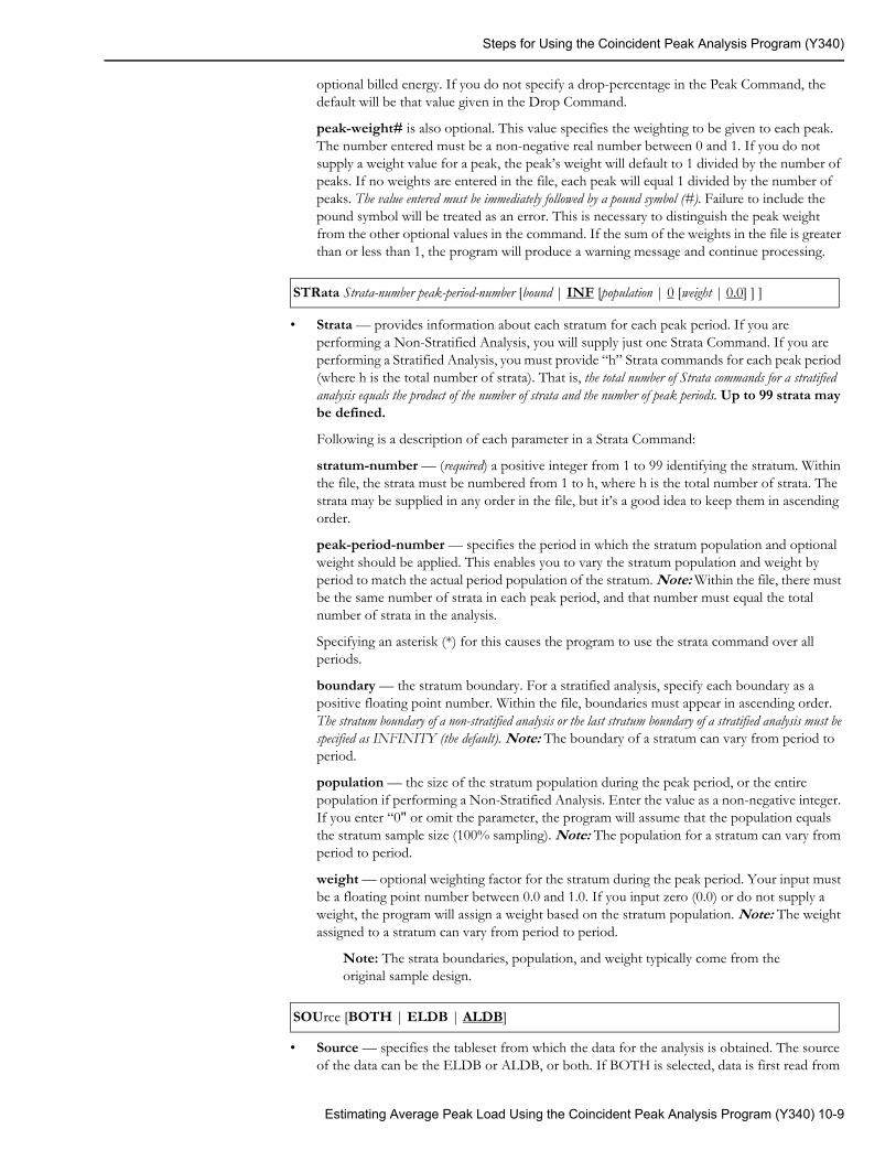
Steps for Using the Coincident Peak Analysis Program (Y340)
optional billed energy. If you do not specify a drop-percentage in the Peak Command, the default will be that value given in the Drop Command.
peak-weight# is also optional. This value specifies the weighting to be given to each peak. The number entered must be a non-negative real number between 0 and 1. If you do not supply a weight value for a peak, the peak’s weight will default to 1 divided by the number of peaks. If no weights are entered in the file, each peak will equal 1 divided by the number of peaks. The value entered must be immediately followed by a pound symbol (#). Failure to include the pound symbol will be treated as an error. This is necessary to distinguish the peak weight from the other optional values in the command. If the sum of the weights in the file is greater than or less than 1, the program will produce a warning message and continue processing.
• Strata — provides information about each stratum for each peak period. If you are performing a Non-Stratified Analysis, you will supply just one Strata Command. If you are performing a Stratified Analysis, you must provide “h” Strata commands for each peak period (where h is the total number of strata). That is, the total number of Strata commands for a stratified analysis equals the product of the number of strata and the number of peak periods. Up to 99 strata may be defined.
Following is a description of each parameter in a Strata Command:
stratum-number — (required) a positive integer from 1 to 99 identifying the stratum. Within the file, the strata must be numbered from 1 to h, where h is the total number of strata. The strata may be supplied in any order in the file, but it’s a good idea to keep them in ascending order.
peak-period-number — specifies the period in which the stratum population and optional weight should be applied. This enables you to vary the stratum population and weight by period to match the actual period population of the stratum. Note: Within the file, there must be the same number of strata in each peak period, and that number must equal the total number of strata in the analysis.
Specifying an asterisk (*) for this causes the program to use the strata command over all periods.
boundary — the stratum boundary. For a stratified analysis, specify each boundary as a positive floating point number. Within the file, boundaries must appear in ascending order. The stratum boundary of a non-stratified analysis or the last stratum boundary of a stratified analysis must be specified as INFINITY (the default). Note: The boundary of a stratum can vary from period to period.
population — the size of the stratum population during the peak period, or the entire population if performing a Non-Stratified Analysis. Enter the value as a non-negative integer. If you enter “0" or omit the parameter, the program will assume that the population equals the stratum sample size (100% sampling). Note: The population for a stratum can vary from period to period.
weight — optional weighting factor for the stratum during the peak period. Your input must be a floating point number between 0.0 and 1.0. If you input zero (0.0) or do not supply a weight, the program will assign a weight based on the stratum population. Note: The weight assigned to a stratum can vary from period to period.
Note: The strata boundaries, population, and weight typically come from the original sample design.
• Source — specifies the tableset from which the data for the analysis is obtained. The source of the data can be the ELDB or ALDB, or both. If BOTH is selected, data is first read from
STRata Strata-number peak-period-number [bound | INF [population | 0 [weight | 0.0] ] ]
SOUrce [BOTH | ELDB | ALDB]
Estimating Average Peak Load Using the Coincident Peak Analysis Program (Y340) 10-9
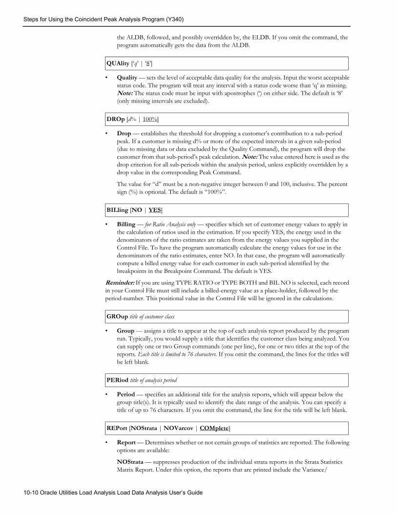
Steps for Using the Coincident Peak Analysis Program (Y340)
the ALDB, followed, and possibly overridden by, the ELDB. If you omit the command, the program automatically gets the data from the ALDB.
• Quality — sets the level of acceptable data quality for the analysis. Input the worst acceptable status code. The program will treat any interval with a status code worse than ‘q’ as missing. Note: The status code must be input with apostrophes (‘) on either side. The default is ‘8’ (only missing intervals are excluded).
• Drop — establishes the threshold for dropping a customer’s contribution to a sub-period peak. If a customer is missing d% or more of the expected intervals in a given sub-period (due to missing data or data excluded by the Quality Command), the program will drop the customer from that sub-period’s peak calculation. Note: The value entered here is used as the drop criterion for all sub-periods within the analysis period, unless explicitly overridden by a drop value in the corresponding Peak Command.
The value for “d” must be a non-negative integer between 0 and 100, inclusive. The percent sign (%) is optional. The default is “100%”.
• Billing — for Ratio Analysis only — specifies which set of customer energy values to apply in the calculation of ratios used in the estimation. If you specify YES, the energy used in the denominators of the ratio estimates are taken from the energy values you supplied in the Control File. To have the program automatically calculate the energy values for use in the denominators of the ratio estimates, enter NO. In that case, the program will automatically compute a billed energy value for each customer in each sub-period identified by the breakpoints in the Breakpoint Command. The default is YES.
Reminder: If you are using TYPE RATIO or TYPE BOTH and BIL NO is selected, each record in your Control File must still include a billed-energy value as a place-holder, followed by the period-number. This positional value in the Control File will be ignored in the calculations.
• Group — assigns a title to appear at the top of each analysis report produced by the program run. Typically, you would supply a title that identifies the customer class being analyzed. You can supply one or two Group commands (one per line), for one or two titles at the top of the reports. Each title is limited to 76 characters. If you omit the command, the lines for the titles will be left blank.
• Period — specifies an additional title for the analysis reports, which will appear below the group title(s). It is typically used to identify the date range of the analysis. You can specify a title of up to 76 characters. If you omit the command, the line for the title will be left blank.
• Report — Determines whether or not certain groups of statistics are reported. The following options are available:
NOStrata — suppresses production of the individual strata reports in the Strata Statistics Matrix Report. Under this option, the reports that are printed include the Variance/
QUAlity [‘q’ | ‘8’]
DROp [d% | 100%]
BILling [NO | YES]
GROup title of customer class
PERiod title of analysis period
REPort [NOStrata | NOVarcov | COMplete]
10-10 Oracle Utilities Load Analysis Load Data Analysis User’s Guide
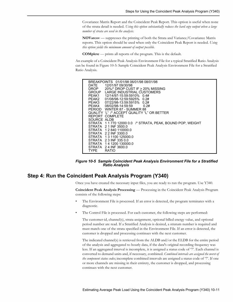
Steps for Using the Coincident Peak Analysis Program (Y340)
Covariance Matrix Report and the Coincident Peak Report. This option is useful when none of the strata detail is needed. Using this option substantially reduces the hard copy output when a large number of strata are used in the analysis.
NOVarcov — suppresses the printing of both the Strata and Variance/Covariance Matrix reports. This option should be used when only the Coincident Peak Report is needed. Using this option yields the minimum amount of output possible.
COMplete — prints all reports of the program. This is the default.
An example of a Coincident Peak Analysis Environment File for a typical Stratified Ratio Analysis can be found in Figure 10-5: Sample Coincident Peak Analysis Environment File for a Stratified Ratio Analysis.
Figure 10-5 Sample Coincident Peak Analysis Environment File for a Stratified Ratio Analysis
Step 4: Run the Coincident Peak Analysis Program (Y340)Once you have created the necessary input files, you are ready to run the program. Use Y340.
Coincident Peak Analysis Processing — Processing in the Coincident Peak Analysis Program consists of the following steps:
• The Environment File is processed. If an error is detected, the program terminates with a diagnostic.
• The Control File is processed. For each customer, the following steps are performed:
The customer-id, channel(s), strata assignment, optional billed energy value, and optional period number are read. If a Stratified Analysis is desired, a stratum number is required and must match one of the strata specified in the Environment File. If an error is detected, the customer is dropped and processing continues with the next customer.
The indicated channel(s) is retrieved from the ALDB and/or the ELDB for the entire period of the analysis and aggregated to hourly data, if the data’s original recording frequency was less. If an aggregated interval is incomplete, it is assigned a status code of ‘7’. Each channel is converted to demand units and, if necessary, combined. Combined intervals are assigned the worst of the component status codes; incomplete combined intervals are assigned a status code of ‘7’. If one or more channels are missing in their entirety, the customer is dropped, and processing continues with the next customer.
BREAKPOINTS 01/01/98 06/01/98 08/01/98DATE 12/01/97 09/30/98DROP 20%/* DROP CUST IF > 20% MISSINGGROUP LARGE INDUSTRIAL CUSTOMERSPEAK1 12/14/97-15:59:5910% 0.4#PEAK2 01/08/98-12:59:5925% 0.2#PEAK3 07/22/98-13:59:5915% 0.2#PEAK4 08/02/98-14:59:59 0.2#PERIOD WINTER 87 - SUMMER 88QUALITY ‘L’ /* ACCEPT QUALITY “L” OR BETTERREPORT COMPLETESOURCE ALDBSTRATA 1 1 770 12000 0.0 /* STRATA, PEAK, BOUND POP, WEIGHTSTRATA 2 1 INF 3500.0STRATA 1 2 840 110000.0STRATA 2 2 INF 3300.0STRATA 1 3 1100 125000.0STRATA 2 3 INF 335 0.0STRATA 1 4 1200 130000.0STRATA 2 4 INF 3600.0TYPE RATIO
Estimating Average Peak Load Using the Coincident Peak Analysis Program (Y340) 10-11

Steps for Using the Coincident Peak Analysis Program (Y340)
• The customer’s peak data is scanned for quality. If a peak interval’s status code exceeds the quality code specified in the Environment File, the interval is set to zero and flagged as missing.
• The customer’s combined demand array for the entire analysis period is divided into sub-periods based upon the entered breakpoints. For each sub-period including a peak value, the entire set of data is scanned for missing data or data excluded due to unacceptable quality. If the percentage of excluded data (relative to the total sub-period data) is above that peak period’s drop criterion, the peak value for that period is dropped from the analysis. Testing continues with the next sub-period that includes a peak, until all sub-periods have been examined. If a customer has at least one peak value, it is included in the analysis.
• The following statistics are calculated for the peak periods in the analysis by strata:
Mean demand (row and column)
Standard error of the mean demand
Correlation coefficient
Average sample size
Common sample size.
• Total variance/covariance statistics calculated for the peak periods in the analysis (summed over strata) are:
The Variances of the coincident peak demands for average and customer class levels
The Co-variances of the coincident peak demands for average and customer class levels.
• Coincident peak statistics are calculated for the peak periods in the analysis and for the entire period of analysis. These statistics are:
Average customer-level coincident peak demand
Variance of the average customer-level coincident peak demand
Contribution to variance of the individual variances of the period average customer-level coincident peak demands
Contribution to variance of the individual co-variances of the between period average customer-level coincident peak demands
Standard error of the average customer-level coincident peak demand
Customer class-level coincident peak demand
Variance of the customer class-level coincident peak demand
Contribution to variance of the individual variances of the period customer class-level coincident peak demands
Contribution to variance of the individual co-variances of the between period customer class-level coincident peak demands
Standard error of the customer class-level coincident peak demand.
10-12 Oracle Utilities Load Analysis Load Data Analysis User’s Guide
Chapter 11Estimating Loads for Subpopulations Using the
Domains Analysis Programs (Y350 or Y360)
Domains analysis is used to study the load characteristics of subpopulations within a customer class — for example, residential customers with water heaters, or grocery stores that stay open 24 hours a day. This technique maximizes the value of existing load research data by making it possible to study subpopulations, or domains, other than those for which a sample was originally designed. It is extremely useful for rate design, demand side management, forecasting, and marketing studies.
Two optional Oracle Utilities Load Analysis extensions are available in the Analysis Bundle to perform domains analysis: the Domains Analysis Mean Per Unit Program (Y350) and the Domains Analysis Ratio Program (Y360). Both versions are described in this manual.
Topics covered in this manual:
• The Domains Analysis Programs
• Steps for Using the Domains Analysis Program (Y350 or Y360)
Estimating Loads for Subpopulations Using the Domains Analysis Programs (Y350 or Y360) 11-1
The Domains Analysis Programs
The Domains Analysis ProgramsThe Domains Analysis programs are used to compute load statistics for one or more subpopulations, or domains, within an analysis group. These subpopulations are selected from an existing load research sample, but are different from those used in designing the original sample. Two programs are available for domains analysis: Domains Analysis Mean-Per-Unit (Domains MPU) and Domains Analysis Ratio (Domains Ratio).
Both programs perform either stratified or non-stratified analyses and analyze a set of domains over an existing stratification scheme. Periods of up to one year may be analyzed, and holidays, time-of-use periods, and type-of-day definitions are incorporated. Up to thirty-five (35) different domains may be analyzed in one job run.
Expansion MethodsDomains MPU — Two methods of expansion are implemented by the Domains MPU Program. The preferred method is the use of domain populations for the expansion estimates. This requires knowledge of the population totals for each domain within each stratum, and should provide the most accurate results. The second technique is employed when populations are not known within each domain. In that case, the expansion is performed using the total population. The equations used for both methods are provided in Appendix G, “Domains Analysis Mean Per Unit Equations”, in the Oracle Utilities Load Analysis Load Data Analysis User’s Guide.
With Domains Ratio, stratified analysis results are calculated using the Combined Estimate technique. This estimation technique is based on the ratio of domain demand to domain energy when total billed energy is available for each domain; otherwise, the ratio of domain demand to sample energy is used to estimate the total.
ResultsBoth programs calculate estimates of coincident demands, non-coincident demands, and energy. For Domains MPU, these estimates are in the form of total demand based on a mean per unit structure, and are provided for the customer, strata, domain, and population levels within an analysis group. For Domains Ratio, these estimates are in the form of total demand based on a ratio estimate, and are provided for the customer, domain, and population levels within an analysis group. Domains Ratio additionally calculates load factors and diversity factors (Domains MPU does not).
Both programs produce time-of-use and type-of-day statistics. Estimates of the relative accuracy of each statistic are computed for sample evaluation. Statistics may be written to the ELDB for additional evaluation, reporting, and archiving to the SLDB. A file of individual customer statistics, which can be accessed by user programs, is also created by both programs.
11-2 Oracle Utilities Load Analysis Load Data Analysis User’s Guide
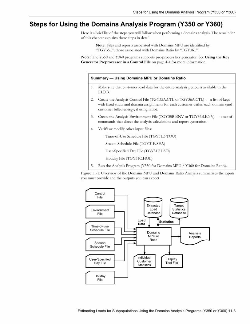
Steps for Using the Domains Analysis Program (Y350 or Y360)
Steps for Using the Domains Analysis Program (Y350 or Y360)Here is a brief list of the steps you will follow when performing a domains analysis. The remainder of this chapter explains these steps in detail.
Note: Files and reports associated with Domains MPU are identified by “TGY35_”; those associated with Domains Ratio by “TGY36_”.
Note: The Y350 and Y360 programs supports pre-process key generator. See Using the Key Generator Preprocessor in a Control File on page 4-4 for more information.
Figure 11-1: Overview of the Domains MPU and Domains Ratio Analysis summarizes the inputs you must provide and the outputs you can expect.
Summary — Using Domains MPU or Domains Ratio
1. Make sure that customer load data for the entire analysis period is available in the ELDB.
2. Create the Analysis Control File (TGY35A.CTL or TGY36A.CTL) — a list of keys with fixed strata and domain assignments for each customer within each domain (and customer billed energy, if using ratio).
3. Create the Analysis Environment File (TGY35B.ENV or TGY36B.ENV) — a set of commands that direct the analysis calculations and report generation.
4. Verify or modify other input files:
Time-of-Use Schedule File (TGY31D.TOU)
Season Schedule File (TGY31E.SEA)
User-Specified Day File (TGY31F.USD)
Holiday File (TGY31C.HOL)
5. Run the Analysis Program (Y350 for Domains MPU / Y360 for Domains Ratio).
SeasonSchedule File
User-Specified Day File
DomainsMPU orRatio
AnalysisReports
IndividualCustomerStatistics
StatisticsLoadData
ControlFile
HolidayFile
EnvironmentFile
Time-of-useSchedule File
ExtractedLoad
Database
TargetStatisticsDatabase
Display Tool File
Estimating Loads for Subpopulations Using the Domains Analysis Programs (Y350 or Y360) 11-3
Steps for Using the Domains Analysis Program (Y350 or Y360)
Figure 11-1 Overview of the Domains MPU and Domains Ratio Analysis
Step 1: Ensure Data is Available in the ELDBPrior to running the analysis, be sure that the ELDB contains reliable load data for all representatives of the domain over the entire analysis period. (Chapter 5 of the Oracle Utilities Load Analysis Load Data Analysis User’s Guide provides detailed instructions for getting data in the ELDB.) You may wish to run the ELDB Summary Reporter (Y440) to verify that the desired data is available.
Other requirements for load data are the same as those for Standard Load Analysis (see Step 1 in Chapter 7 of the Oracle Utilities Load Analysis Load Data Analysis User’s Guide).
Step 2: Create the Analysis Control File (TGY35A.CTL or TGY36A.CTL)The Analysis Control File is a list of keys identifying the customers to be analyzed, along with their strata and domain assignments. If you are using the Domains Analysis Ratio Program, you may also provide billed-energy values for each customer.
Note: If you have set up your descriptor to include required information, then you can use Key Generator to perform queries and create query lists.
Strata assignments typically come from the original sample design. Domain assignments, on the other hand, must be determined externally. That is, because the definition of the domain(s) typically post-dates the sample design, you will have to determine whether or not each customer belongs to a domain, based on characteristic data obtained via surveys or other methods. The Customer Data Extraction (CDE) Program can be a useful tool for this process. That program, which is described later in this manual, enables you to create a file of customers that match a set of user-specified criteria (as long as the defining characteristics are captured in the Customer Attribute File). Other options for creating the Control File are to type it manually, or to use the Key Generator Program to create a file of customers based on fields in the Oracle Utilities Load Data Records (the Key Generator programs are described later in this manual).
Billed energy (for ratio only) typically comes from “Billing.” If you cannot provide customer billed energy, you can have the program calculate the values from interval data in the Interval Database. (This is explained further later in the chapter.) Another alternative is to use the Billed Energy Program to calculate customer billed energy by billing cycles. This is the preferred approach, and is explained in Chapter 14, “Computing Customer Energy Use by Billing Cycles Using the Billed Energy Program (Y230),” in the Oracle Utilities Load Analysis Load Data Analysis User’s Guide.
(Note about combining channels into single sample points: The Analysis Control File allows you to combine multiple channels of data for a single customer-id into a single “cut” for analysis. If you want to combine multiple customer-ids for a large individual customer to create a single sample point, you will have to use the Transformation Program or the Billed Energy Program prior to analysis.)
No matter which method you use to construct the Control File, it must consist of a series of control records that conform to the format specified below, with one record for each sample point. You may input spaces and/or a comma between elements in the command record, with the exception that blanks are not allowed before or after an operator if combining channels.
Note: The energy units-of-measure of all customers in the Analysis Control File must be compatible with each other. Groups of compatible units-of-measure (i.e., different units that may be analyzed together) are listed in Appendix I of the Oracle Utilities Load Analysis Load Data Analysis User’s Guide.
Control File Record Format for Domains MPU
customer-id chan1 [{±}chan2 [{±}chan3...[{±}chann ] ] ] strata-number [domain]
11-4 Oracle Utilities Load Analysis Load Data Analysis User’s Guide
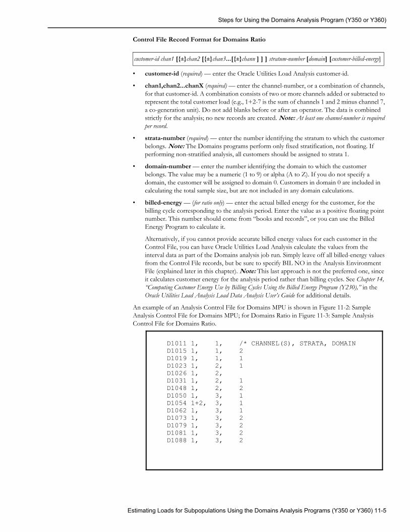
Steps for Using the Domains Analysis Program (Y350 or Y360)
Control File Record Format for Domains Ratio
• customer-id (required) — enter the Oracle Utilities Load Analysis customer-id.
• chan1,chan2...chanX (required) — enter the channel-number, or a combination of channels, for that customer-id. A combination consists of two or more channels added or subtracted to represent the total customer load (e.g., 1+2-7 is the sum of channels 1 and 2 minus channel 7, a co-generation unit). Do not add blanks before or after an operator. The data is combined strictly for the analysis; no new records are created. Note: At least one channel-number is required per record.
• strata-number (required) — enter the number identifying the stratum to which the customer belongs. Note: The Domains programs perform only fixed stratification, not floating. If performing non-stratified analysis, all customers should be assigned to strata 1.
• domain-number — enter the number identifying the domain to which the customer belongs. The value may be a numeric (1 to 9) or alpha (A to Z). If you do not specify a domain, the customer will be assigned to domain 0. Customers in domain 0 are included in calculating the total sample size, but are not included in any domain calculations.
• billed-energy — (for ratio only) — enter the actual billed energy for the customer, for the billing cycle corresponding to the analysis period. Enter the value as a positive floating point number. This number should come from “books and records”, or you can use the Billed Energy Program to calculate it.
Alternatively, if you cannot provide accurate billed energy values for each customer in the Control File, you can have Oracle Utilities Load Analysis calculate the values from the interval data as part of the Domains analysis job run. Simply leave off all billed-energy values from the Control File records, but be sure to specify BIL NO in the Analysis Environment File (explained later in this chapter). Note: This last approach is not the preferred one, since it calculates customer energy for the analysis period rather than billing cycles. See Chapter 14, “Computing Customer Energy Use by Billing Cycles Using the Billed Energy Program (Y230),” in the Oracle Utilities Load Analysis Load Data Analysis User’s Guide for additional details.
An example of an Analysis Control File for Domains MPU is shown in Figure 11-2: Sample Analysis Control File for Domains MPU; for Domains Ratio in Figure 11-3: Sample Analysis Control File for Domains Ratio.
customer-id chan1 [{±}chan2 [{±}chan3...[{±}chann ] ] ] stratum-number [domain] [customer-billed-energy]
D1011 1, 1, /* CHANNEL(S), STRATA, DOMAIND1015 1, 1, 2D1019 1, 1, 1D1023 1, 2, 1D1026 1, 2,D1031 1, 2, 1D1048 1, 2, 2D1050 1, 3, 1D1054 1+2, 3, 1D1062 1, 3, 1D1073 1, 3, 2D1079 1, 3, 2D1081 1, 3, 2D1088 1, 3, 2
Estimating Loads for Subpopulations Using the Domains Analysis Programs (Y350 or Y360) 11-5
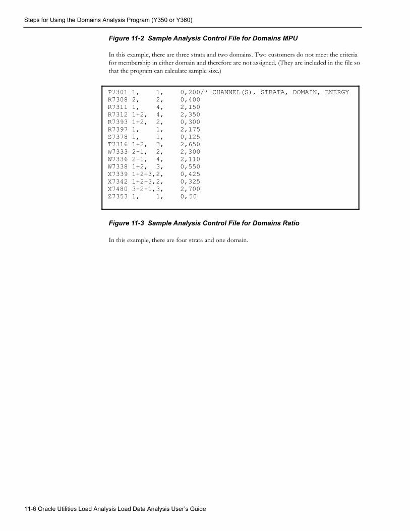
Steps for Using the Domains Analysis Program (Y350 or Y360)
Figure 11-2 Sample Analysis Control File for Domains MPU
In this example, there are three strata and two domains. Two customers do not meet the criteria for membership in either domain and therefore are not assigned. (They are included in the file so that the program can calculate sample size.).
Figure 11-3 Sample Analysis Control File for Domains Ratio
In this example, there are four strata and one domain.
P7301 1, 1, 0,200/* CHANNEL(S), STRATA, DOMAIN, ENERGYR7308 2, 2, 0,400R7311 1, 4, 2,150R7312 1+2, 4, 2,350R7393 1+2, 2, 0,300R7397 1, 1, 2,175S7378 1, 1, 0,125T7316 1+2, 3, 2,650W7333 2-1, 2, 2,300W7336 2-1, 4, 2,110W7338 1+2, 3, 0,550X7339 1+2+3,2, 0,425X7342 1+2+3,2, 0,325X7480 3-2-1,3, 2,700Z7353 1, 1, 0,50
11-6 Oracle Utilities Load Analysis Load Data Analysis User’s Guide
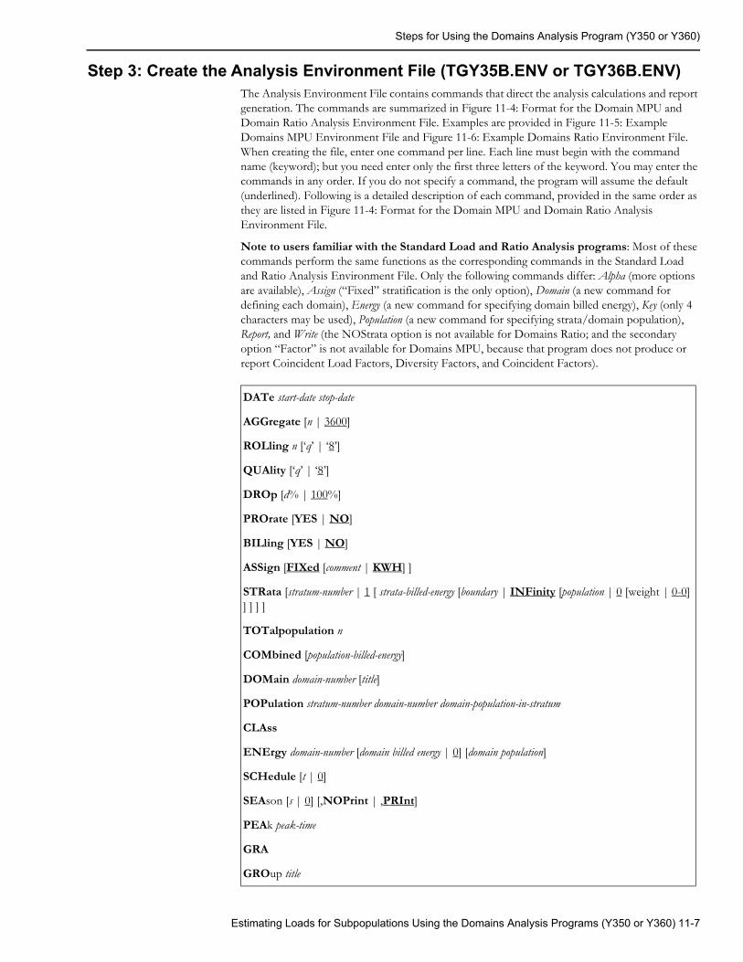
Steps for Using the Domains Analysis Program (Y350 or Y360)
Step 3: Create the Analysis Environment File (TGY35B.ENV or TGY36B.ENV)The Analysis Environment File contains commands that direct the analysis calculations and report generation. The commands are summarized in Figure 11-4: Format for the Domain MPU and Domain Ratio Analysis Environment File. Examples are provided in Figure 11-5: Example Domains MPU Environment File and Figure 11-6: Example Domains Ratio Environment File. When creating the file, enter one command per line. Each line must begin with the command name (keyword); but you need enter only the first three letters of the keyword. You may enter the commands in any order. If you do not specify a command, the program will assume the default (underlined). Following is a detailed description of each command, provided in the same order as they are listed in Figure 11-4: Format for the Domain MPU and Domain Ratio Analysis Environment File.
Note to users familiar with the Standard Load and Ratio Analysis programs: Most of these commands perform the same functions as the corresponding commands in the Standard Load and Ratio Analysis Environment File. Only the following commands differ: Alpha (more options are available), Assign (“Fixed” stratification is the only option), Domain (a new command for defining each domain), Energy (a new command for specifying domain billed energy), Key (only 4 characters may be used), Population (a new command for specifying strata/domain population), Report, and Write (the NOStrata option is not available for Domains Ratio; and the secondary option “Factor” is not available for Domains MPU, because that program does not produce or report Coincident Load Factors, Diversity Factors, and Coincident Factors).
DATe start-date stop-date
AGGregate [n | 3600]
ROLling n [‘q’ | ‘8’]
QUAlity [‘q’ | ‘8’]
DROp [d% | 100%]
PROrate [YES | NO]
BILling [YES | NO]
ASSign [FIXed [comment | KWH] ]
STRata [stratum-number | 1 [ strata-billed-energy [boundary | INFinity [population | 0 [weight | 0-0] ] ] ] ]
TOTalpopulation n
COMbined [population-billed-energy]
DOMain domain-number [title]
POPulation stratum-number domain-number domain-population-in-stratum
CLAss
ENErgy domain-number [domain billed energy | 0] [domain population]
SCHedule [t | 0]
SEAson [s | 0] [,NOPrint | ,PRInt]
PEAk peak-time
GRA
GROup title
Estimating Loads for Subpopulations Using the Domains Analysis Programs (Y350 or Y360) 11-7
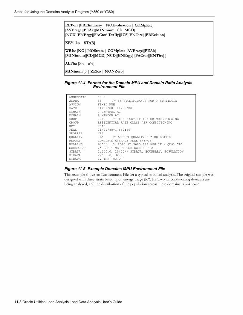
Steps for Using the Domains Analysis Program (Y350 or Y360)
Figure 11-4 Format for the Domain MPU and Domain Ratio Analysis Environment File
Figure 11-5 Example Domains MPU Environment FileThis example shows an Environment File for a typical stratified analysis. The original sample was designed with three strata based upon energy usage (KWH). Two air conditioning domains are being analyzed, and the distribution of the population across these domains is unknown.
REPort [PREliminary | NOEvaluation | COMplete] [AVErage][PEAk][MINimum][CD][MCD] [NCD][ENErgy][FACtor][DAIly][ICS][ENTire] [PREcision]
KEY [key | STAR]
WRIte [NO| NOStrata | COMplete [AVErage][PEAk] [MINimum][CD][MCD][NCD][ENErgy] [FACtor][ENTire] ]
ALPha [5% | n%]
MINinum [0 | ZERo | NONZero]
AGGREGATE 1800ALPHA 5% /* 5% SIGNIFICANCE FOR T-STATISTICASSIGN FIXED KWHDATE 11/01/88 11/30/88DOMAIN 1 CENTRAL ACDOMAIN 2 WINDOW ACDROP 10% /* DROP CUST IF 10% OR MORE MISSINGGROUP RESIDENTIAL RATE CLASS AIR CONDITIONINGKEY RSACPEAK 11/21/88-17:59:59PRORATE YESQUALITY ‘L’ /* ACCEPT QUALITY “L” OR BETTERREPORT COMPLETE AVERAGE PEAK ENERGYROLLING 60‘L’ /* ROLL AT 3600 SPI AGG IF < QUAL “L”SCHEDULE2 /* USE TIME-OF-USE SCHEDULE 2STRATA 1,350.0, 10400/* STRATA, BOUNDARY, POPULATIONSTRATA 2,600.0, 32790STRATA 3, INF, 8370
11-8 Oracle Utilities Load Analysis Load Data Analysis User’s Guide
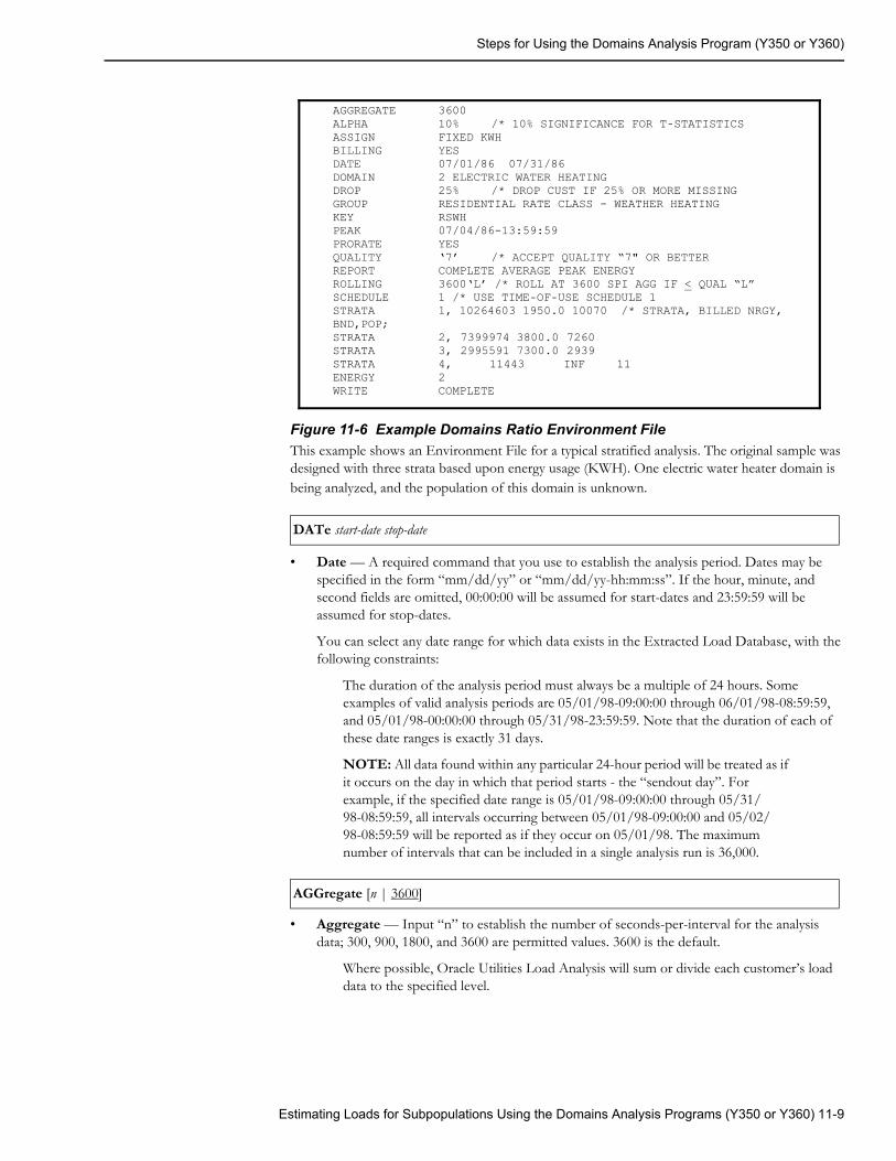
Steps for Using the Domains Analysis Program (Y350 or Y360)
Figure 11-6 Example Domains Ratio Environment FileThis example shows an Environment File for a typical stratified analysis. The original sample was designed with three strata based upon energy usage (KWH). One electric water heater domain is being analyzed, and the population of this domain is unknown.
• Date — A required command that you use to establish the analysis period. Dates may be specified in the form “mm/dd/yy” or “mm/dd/yy-hh:mm:ss”. If the hour, minute, and second fields are omitted, 00:00:00 will be assumed for start-dates and 23:59:59 will be assumed for stop-dates.
You can select any date range for which data exists in the Extracted Load Database, with the following constraints:
The duration of the analysis period must always be a multiple of 24 hours. Some examples of valid analysis periods are 05/01/98-09:00:00 through 06/01/98-08:59:59, and 05/01/98-00:00:00 through 05/31/98-23:59:59. Note that the duration of each of these date ranges is exactly 31 days.
NOTE: All data found within any particular 24-hour period will be treated as if it occurs on the day in which that period starts - the “sendout day”. For example, if the specified date range is 05/01/98-09:00:00 through 05/31/98-08:59:59, all intervals occurring between 05/01/98-09:00:00 and 05/02/98-08:59:59 will be reported as if they occur on 05/01/98. The maximum number of intervals that can be included in a single analysis run is 36,000.
• Aggregate — Input “n” to establish the number of seconds-per-interval for the analysis data; 300, 900, 1800, and 3600 are permitted values. 3600 is the default.
Where possible, Oracle Utilities Load Analysis will sum or divide each customer’s load data to the specified level.
DATe start-date stop-date
AGGregate [n | 3600]
AGGREGATE 3600ALPHA 10% /* 10% SIGNIFICANCE FOR T-STATISTICSASSIGN FIXED KWHBILLING YESDATE 07/01/86 07/31/86DOMAIN 2 ELECTRIC WATER HEATINGDROP 25% /* DROP CUST IF 25% OR MORE MISSINGGROUP RESIDENTIAL RATE CLASS - WEATHER HEATINGKEY RSWHPEAK 07/04/86-13:59:59PRORATE YESQUALITY ‘7’ /* ACCEPT QUALITY “7" OR BETTERREPORT COMPLETE AVERAGE PEAK ENERGYROLLING 3600‘L’ /* ROLL AT 3600 SPI AGG IF < QUAL “L”SCHEDULE 1 /* USE TIME-OF-USE SCHEDULE 1STRATA 1, 10264603 1950.0 10070 /* STRATA, BILLED NRGY, BND,POP;STRATA 2, 7399974 3800.0 7260STRATA 3, 2995591 7300.0 2939STRATA 4, 11443 INF 11ENERGY 2WRITE COMPLETE
Estimating Loads for Subpopulations Using the Domains Analysis Programs (Y350 or Y360) 11-9
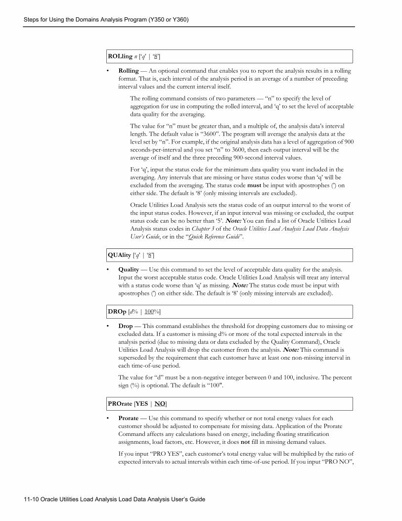
Steps for Using the Domains Analysis Program (Y350 or Y360)
• Rolling — An optional command that enables you to report the analysis results in a rolling format. That is, each interval of the analysis period is an average of a number of preceding interval values and the current interval itself.
The rolling command consists of two parameters — “n” to specify the level of aggregation for use in computing the rolled interval, and ‘q’ to set the level of acceptable data quality for the averaging.
The value for “n” must be greater than, and a multiple of, the analysis data’s interval length. The default value is “3600”. The program will average the analysis data at the level set by “n”. For example, if the original analysis data has a level of aggregation of 900 seconds-per-interval and you set “n” to 3600, then each output interval will be the average of itself and the three preceding 900-second interval values.
For ‘q’, input the status code for the minimum data quality you want included in the averaging. Any intervals that are missing or have status codes worse than ‘q’ will be excluded from the averaging. The status code must be input with apostrophes (’) on either side. The default is ‘8’ (only missing intervals are excluded).
Oracle Utilities Load Analysis sets the status code of an output interval to the worst of the input status codes. However, if an input interval was missing or excluded, the output status code can be no better than ‘5’. Note: You can find a list of Oracle Utilities Load Analysis status codes in Chapter 3 of the Oracle Utilities Load Analysis Load Data Analysis User’s Guide, or in the “Quick Reference Guide”.
• Quality — Use this command to set the level of acceptable data quality for the analysis. Input the worst acceptable status code. Oracle Utilities Load Analysis will treat any interval with a status code worse than ‘q’ as missing. Note: The status code must be input with apostrophes (’) on either side. The default is ‘8’ (only missing intervals are excluded).
• Drop — This command establishes the threshold for dropping customers due to missing or excluded data. If a customer is missing d% or more of the total expected intervals in the analysis period (due to missing data or data excluded by the Quality Command), Oracle Utilities Load Analysis will drop the customer from the analysis. Note: This command is superseded by the requirement that each customer have at least one non-missing interval in each time-of-use period.
The value for “d” must be a non-negative integer between 0 and 100, inclusive. The percent sign (%) is optional. The default is “100".
• Prorate — Use this command to specify whether or not total energy values for each customer should be adjusted to compensate for missing data. Application of the Prorate Command affects any calculations based on energy, including floating stratification assignments, load factors, etc. However, it does not fill in missing demand values.
If you input “PRO YES”, each customer’s total energy value will be multiplied by the ratio of expected intervals to actual intervals within each time-of-use period. If you input “PRO NO”,
ROLling n [‘q’ | ‘8’]
QUAlity [‘q’ | ‘8’]
DROp [d% | 100%]
PROrate [YES | NO]
11-10 Oracle Utilities Load Analysis Load Data Analysis User’s Guide
Steps for Using the Domains Analysis Program (Y350 or Y360)
Oracle Utilities Load Analysis will make no adjustments for missing or excluded data. NO is the default.
• Billing — for Ratio only — This command enables you to specify the energy values for individual sample customers that Oracle Utilities Load Analysis will use to compute the ratio denominator of the ratio estimate. If you specify “YES,” Oracle Utilities Load Analysis will use the billed-energy values you supplied in the Control File. If you specify “NO”, the program will automatically calculate energy values for each customer-id from the recorded interval data in the Oracle Utilities Load Analysis tableset. “NO” is the default. “BIL YES” must be specified to produce the Billed Energy Summary Report.
Reminder: if you specify “YES”, you must supply actual customer billed energy values in the Control File.
• Assign — This command indicates the method by which customers are assigned to strata. Since the Domains Program requires that the strata assignments be fixed, you must indicate FIXed. This means that the program will use the strata assignments you supplied in the Control File. If desired, use the comment field to note the criteria that were the basis for the strata assignments. Input up to 12 characters, with no intervening blanks. The default is KWH (this is simply a comment; it does not affect processing).
• Strata — Provides information about each stratum in the analysis. How you set up the Strata Command(s) largely determines what kind of analysis the program performs. Generally, you will supply one Strata Command for each stratum in a stratified analysis. If you supply just one Strata Command in the file, the program will perform a non-stratified analysis. If you leave out the command altogether, the program will perform the default: non-stratified analysis of a 100% sampled population.
Parameters you supply within the command further influence the type of analysis, as explained below.
Input one command (line) for each stratum in the analysis. Up to 99 strata may be defined. The following explains each parameter in the command:
stratum-number — Identifies the stratum. It must be a positive integer from 1 to 99. Within the file, stratum numbers must appear in consecutive order starting with “1”. For a non-stratified analysis, use a single Strata Command specifying stratum number 1.
stratum-billed-energy (For Ratio only) — Input the actual total billed energy for the stratum population as a positive floating point number. Note: Stratum-billed-energy is required even if you set the Billing Option to NO (see the Billing Command, earlier in this section).
boundary — Defines the upper boundary of the stratum.
For a non-stratified analysis — Specify the stratum boundary as “INF”.
For a pre-stratified analysis — You may use this position in the command for comments. Your comments can consist of up to 12 characters with no intervening blanks.
For a stratified analysis — Specify “INFinity” as the boundary for the last stratum.
BILling [YES | NO]
ASSign [FIXed [comment | KWH] ]
STRata [stratum-number | 1 [ strata-billed-energy [boundary | INFinity [population | 0 [weight | 0-0] ] ] ] ]
Estimating Loads for Subpopulations Using the Domains Analysis Programs (Y350 or Y360) 11-11
Steps for Using the Domains Analysis Program (Y350 or Y360)
population — the size of the stratum population, or the entire population if performing a non-stratified analysis. If you input “0” or omit the parameter, Oracle Utilities Load Analysis will assume that the population equals the stratum sample size (100% sampling).
weight — optional weighting factor for the stratum. Your input must be a floating point number between zero and one. If you input zero (0.0) or do not supply a weight, Oracle Utilities Load Analysis will assign a weight based on the stratum population.
Note: The strata boundaries, population, and weight typically come from the original sample design criteria.
• Totalpopulation: When this command is supplied, if any integers have been assigned in the strata population command, the TOTalpopulation calculations will override the user-supplied values. The value of n must be a non-negative integer.
When this happens, that line of the environment file report will be flagged with an asterisk and a legend will appear at the bottom of the report that will read:
“*The supplied strata population has been overridden by the TOTalpopulation command.”
When the TOT command is in effect, the title of the POPULATION column in the environment report is changed to “CALCULATED POPULATION”.
When using the TOT command, the user must include a place holder of zero (0) for the strata populations to avoid the override messages in the environment report.
If both the strata populations and the strata weights are omitted from the strata commands, and the TOT command is present and valid, the system will equally allocate the total population supplied across the stratus and indicate this in the environment report.
When the user supplies a TOT value in the Environment file, and the strata populations but omits the weights, the program assigns weights as documented and then adjusts the strata populations according to the assigned weights.
The strata populations are calculated using the following formula. The Class Population is supplied via the new TOT n environment file command.
Strata Population = Class Population * Strata weight.
• Combined (optional, for ratio only) — Use this command to supply the actual total billed energy for the entire population, instead of using the Strata Command’s stratum-billed-energy field to allocate the population billed energy across individual strata. Input the value as a positive floating point number. When you supply this command, stratum-billed-energy on Strata commands is ignored.
• Domain — Use this command to define a domain for analysis. Within a single Environment File, you can supply from 1 to 34 Domain commands. Each domain you define in the file will be analyzed in the program run. The population of all domains defined in the file must be mutually exclusive.
One Domain Command is required for each domain included in the analysis period. Multiple Domain commands must be specified in ascending order, with numeric domain-numbers preceding alphabetic; gaps in the sequence are permitted. The command consists of the keyword DOMain and the following parameters:
TOTalpopulation n
COMbined [population-billed-energy]
DOMain domain-number [title]
11-12 Oracle Utilities Load Analysis Load Data Analysis User’s Guide
Steps for Using the Domains Analysis Program (Y350 or Y360)
domain-number (required) — Must be either an integer from 1 to 9 or a single letter of the alphabet (A to Y); domain Z is reserved for optional class totals. This provides for a maximum of 34 domains. Note: The domain-numbers in the Environment File must correspond to the domain-numbers you used in the Control File.
title (optional) — a string of not more than 74 characters that will appear in the heading of each report.
• Class (optional) — Use this command to request an additional set of reports and/or statistics for the entire class of customers (sample) being analyzed, including customers in all domains and those in no domain (domain 0). Results will be comparable to those obtained from a non-domains Standard Analysis (Y310) or Ratio Analysis (Y330) run with the same sample and similar Environment File commands.
• Population (optional) — Use this command to define the population of a domain within a stratum for the time period of the analysis.
If performing Domains MPU: If you supply domain population, the program will use this value to expand the mean and class totals. This is the preferred method, and should provide the most accurate estimates. If you do not supply domain population, or if you specify a zero population, the program will use the strata populations for class expansion. (See the equations in Appendix G of the Oracle Utilities Load Analysis Load Data Analysis User’s Guide for further information.)
If performing Domains Ratio: If you supply domain population, the program will report the value in the Environment File Report, and will use the domain population to calculate the mean (average) demand. If you do not supply any values, the program will print the message “Domain Populations Unknown” in the report.
For either type of analysis, you can enter the Population commands in any sequence, but you can have no more than one Population Command for each stratum/domain combination in the analysis. Each command consists of the keyword POPulation and the following parameters:
stratum-number — the identifier for a stratum that you originally defined using a Strata Command.
domain-number — the identifier for a domain that you originally defined using a Domain Command.
domain-population-in-stratum — a non-negative integer specifying the population of the indicated domain in the indicated stratum. This information is usually obtained from customer survey information.
• Energy (optional, for ratio only) — Use to specify the actual (estimated or computed) billed energy for a particular domain. If no domain billed energy information is available, you can omit this command and the billed energy will default to zero. The command consists of the keyword ENErgy and the following parameters:
domain-number — the identifier for a domain that you originally defined using a Domain Command.
domain-billed-energy — known or estimated total billed energy for the domain, specified as a positive floating point number.
CLAss
POPulation stratum-number domain-number domain-population-in-stratum
ENErgy domain-number [domain billed energy | 0] [domain population]
Estimating Loads for Subpopulations Using the Domains Analysis Programs (Y350 or Y360) 11-13
Steps for Using the Domains Analysis Program (Y350 or Y360)
domain-population (optional) — the population of the entire domain, across all strata. This is a quick alternative to supplying domain populations by strata using the Population Command, above. This alternative supersedes the Population Command; any Population commands left in the Environment File will be ignored, and an informational message printed. If you wish to enter domain population this way, without entering billed energy, code 0 as the domain-billed-energy parameter.
• Schedule — Use to select a single schedule from the Time-of-Use Schedule File (TGY31D) for the time-of-use calculations. The parameter “t” is a non-negative integer representing a particular schedule in your TOU file. The default, “SCHedule 0”, automatically defines a single time-of-use period equal to the analysis period.
Note about the Time-of-Use Schedule File: Instructions for modifying or adding new schedules to the Time-of-Use File are provided in Step 4 of Chapter 7, “Expanding Load Data to Class-Level Estimates Using the Load Analysis Programs (Y310 and Y330)”, in the Oracle Utilities Load Analysis Load Data Analysis User’s Guide. It is very important to keep in mind that any schedule you select must cover the entire analysis period you specified with the DATe Command. If the program encounters a gap, it will stop processing and issue a warning message.
• Season — Use this command to select a schedule from the Season Schedule File (TGY31E) for the time-of-use calculations. Specifying a Season Schedule makes it possible to apply different Time-of-Use schedules to different portions of the analysis period.
The parameter “s” is a non-negative integer representing a particular Season Schedule within the Season Schedule File. The default, “SEASON 0”, indicates that a single Time-of-Use Schedule, as specified in the SCHEDULE Command, is to be applied over the entire analysis period.
The PRINT option indicates that graphs of time-of-use periods are to be printed with the Analysis Environment Report; the NOPRINT option suppresses the printing of these graphs. The default is PRINT.
Note: Either the Season Command or the Schedule Command may be used to define time-of-use periods for analysis processing, but not both. If you include both commands in the Environment File, the program will use the Season Command and disregard the Schedule Command. If you include neither command, the default is “SCHEDULE 0, NOPRINT”.
About the Season Schedule File: Instructions for modifying or adding new schedules to the Season Schedule File are provided in Step 5 of Chapter 7 in the Oracle Utilities Load Analysis Load Data Analysis User’s Guide. It is very important to keep in mind that any schedule you select must cover the entire analysis period you specified with the Date Command. If the program encounters a gap, it will abort processing and issue an error message.
• Peak — This command enables you to specify the date and time of peaks of interest that are not automatically computed by Oracle Utilities Load Analysis – such as system peak. Oracle Utilities Load Analysis will compute statistics for the entire day in which each supplied peak falls.
SCHedule [t | 0]
SEAson [s | 0] [,NOPrint | ,PRInt]
PEAk peak-time
11-14 Oracle Utilities Load Analysis Load Data Analysis User’s Guide
Steps for Using the Domains Analysis Program (Y350 or Y360)
You must use the format “mm/dd/yy-hh:mm:ss” to specify the peak. You can input up to 25 peaks for an MPU Analysis, or up to 23 for a Ratio. Input one peak per line. The default is no peaks.
• GRA - This command determines that a graphics file is produced when running this program.
• Group — Use the Group command to assign a title to appear at the top of each analysis report produced at the end of the program run. You can input one or two Group commands (one per line), for one or two titles at the top of the reports, for the Y360 program; for the Y350 program, you can input one Group command. Each title is limited to 78 characters. Note that using the Group command overwrites the default report name in its first header and the Indexer. If you omit the command, the program supplies specific titles for output reports.
• Report — Use the primary options of this command to specify which groups of statistics Oracle Utilities Load Analysis should calculate and report, and use the secondary options if you wish to print only selected reports. See the tables later in this chapter for a summary of your options.
PREliminary — when you select this option, Oracle Utilities Load Analysis will produce only the Analysis Environment and Individual Customer Statistics reports. This option enables you to preview the analysis results on a customer basis before incurring the overhead associated with a complete analysis.
NOStrata (available for MPU only) — this option produces all report types, but does not report the information on individual strata usually included in the Sample Evaluation Reports. This option is useful when class totals are needed for each interval of the analysis period, but none of the strata detail. This option does not affect the reporting of the major statistics, which still include results broken down by strata.
NOEvaluation — this option suppresses the printing of all components of the Sample Evaluation reports. Since these reports tend to be very lengthy, this option can substantially reduce the size of the hard copy output. Use this option when you want only the major statistics and analysis environment reports.
COMplete — select this option to calculate all statistics and print all reports. This option also produces complete load duration statistics. REPORT COMPLETE is the default.
Use the secondary options if you wish to print only selected reports. The program will still calculate all statistics based on your input for the primary options, but only the specified report(s) will be printed based on the secondary options. For example, if you want to calculate all statistics but print only the Energy Report and Individual Customer Statistics Report, use this command: “REP COM ENE ICS”.
AVErage — prints all average day type evaluation reports.
PEAk — prints all peak day and supplied peak evaluation reports.
MINimum — prints all minimum day reports.
CD — prints the Maximum Coincident Demand Report.
GRA
GROup title
REPort [PREliminary | NOEvaluation | COMplete][AVErage][PEAk] [MINimum][CD][MCD] [NCD][ENErgy][FACtor][DAIly][ICS][ENTire] [PREcision]
Estimating Loads for Subpopulations Using the Domains Analysis Programs (Y350 or Y360) 11-15
Steps for Using the Domains Analysis Program (Y350 or Y360)
MCD — prints the Minimum Coincident Demand Report.
NCD — prints the Noncoincident Demand Report.
ENErgy — prints the Energy Report.
FACtor (for Ratio Analysis only) — prints the Load Factor, Diversity Factor, and Coincidence Factor reports.
DAIly — prints Daily Maximum, Minimum, and Average Demand Report.
PREcision — prints Daily Maximum, Minimum, and Average Accuracy Report.
ICS — prints the Individual Customer Statistics Report.
ENTire — prints the Entire Period Sample Evaluation Report.
• Key — Use the Key Command to assign an identifier to each of the statistics produced by the analysis run. This identifier becomes the prefix in the statistics name (see the “Statistics Identifiers” section in Chapter 3 of the Oracle Utilities Load Analysis Load Data Analysis User’s Guide).
Note: You can use up to 40 characters, the first of which must be alphabetic. A combination of characters (A - Z) and digits (0 - 9) may be used, but special characters (anything that is not a letter or number) are not allowed. The default key is “STAR”.
The program will automatically append the domain-number for which the statistics were computed using the format “Dn” (i.e., STARD1 would be the key for statistics computed for domain 1).
• Write — Use this command to determine which statistics, if any, should be written back to the ELDB.
NO — No statistical records are written back to the ELDB, even if you specify any of the secondary WRITE options. Use this option when you need just the hard copy output reports.
NOStrata (available for MPU only) — Individual strata information for the major statistic reports are written to the ELDB, but individual strata statistics in the Sample Evaluation reports and individual strata level duration statistics are not.
COMplete — Writes all statistical records produced by the analysis run back to the ELDB. This is the default.
Use the secondary options in conjunction with the NOSTRATA or COMPLETE options to write only selected statistics. The program will still calculate all the statistics based on your input for the primary options, but only the specified statistics will be written to the ELDB.
AVErage — writes all average day type statistics, such as average weekday.
PEAk — writes all statistics for peak day and user-supplied peak days.
MINimum — writes all minimum day statistics.
CD — writes Maximum Coincident Demand statistics.
MCD — writes Minimum Coincident Demand statistics.
NCD — writes Maximum Noncoincident Demand statistics.
KEY [key | STAR]
WRIte [NO| NOStrata | COMplete [AVErage][PEAk] [MINimum][CD][MCD][NCD][ENErgy] [FACtor][ENTire] ]
11-16 Oracle Utilities Load Analysis Load Data Analysis User’s Guide
Steps for Using the Domains Analysis Program (Y350 or Y360)
ENErgy — writes Energy statistics.
FACtor — writes statistics corresponding to Load, Diversity, and Coincidence Factors.
ENTire — writes Entire Period statistics.
• Alpha — This command enables you to set the significance level for t-statistics used in the computation of relative precision. The percentage “n” may be 5, 10, 20, 30, 40, 50, or 60. The percent sign (%) is optional.
• MINimum — This command enables you to determine if the Daily Maximum, Minimum, and Average Demands Report will process zero-values as minimums or ignore them as missing. If “0” or “ZERO” is specified, zero-values will be shown as minimums. This might be appropriate, for example, if the analysis is on streetlighting data. “NONZERO” is the default.
Step 4: Verify or Modify Other Required Input FilesAlong with the Control and Environment Files, four other input files may be required for a Domains Analysis (depending upon your selections in the Environment File):
• Holiday File (TGY31C.HOL) — a list of holidays observed in your service territory.
• Time-of-Use Schedule File (TGY31D.TOU) — a series of TOU schedules.
• Season Schedule File (TGY31E.SEA) — a series of season schedules, which enable you to apply different TOU schedules at different times of the year.
• User-Specified Day File (TGY31F.USD) — specifies a group of contiguous or non-contiguous days that may be averaged together for analysis (for example, a set of summer peak days).
Typically, these files are established at system installation and seldom modified. Should you need to update or modify these files (if you want to experiment with a new Time-of-Use Schedule, for example) see steps 4 - 7 of Chapter 7 in the Oracle Utilities Load Analysis Load Data Analysis User’s Guide. Alternatively, you may select local versions of these files, located in your Data directory. Selecting “Default” instructs the program to use the default versions set up by your Oracle Utilities Load Analysis administrator.
Step 5: Run the Analysis ProgramRun Y350 for Domains MPU and Y360 for Domains Ratio. Once you have created and verified the necessary input files, you are ready to run the analysis program.
Domains Analysis Mean Per Unit ProcessingProcessing in the Domains MPU Program follows these steps:
• The Environment File is processed. If an error is detected, the program terminates with a diagnostic message.
• The Holiday File is processed. If an error is detected, the program terminates with a diagnostic message.
• The Time-of-Use File is processed. If an error is detected, the program terminates with a diagnostic message.
ALPha [5% | n%]
MINinum [0 | ZERo | NONZero]
Estimating Loads for Subpopulations Using the Domains Analysis Programs (Y350 or Y360) 11-17

Steps for Using the Domains Analysis Program (Y350 or Y360)
• The Control File is processed. For each customer, the customer-id, channel(s), fixed stratum, and domain number are read. The stratum number must match one of the stratum specified in the Environment File. If no domain number is specified, the customer is assigned to domain zero. If an error is detected, the customer is dropped and processing continues with the next customer.
• For each DOMAIN Command in the Environment File (and for the entire sample, if the Class Command is used) the following steps are performed:
The indicated channel(s) for a customer is retrieved from the ELDB for the analysis period and aggregated accordingly. If an aggregated interval is incomplete, it is assigned a status code of ‘7’. Each channel is converted to energy units and, if necessary, combined. Combined intervals are assigned the worst of the component status codes; incomplete combined intervals are assigned a status code of ‘7’. If one or more channels is missing in its entirety, the customer is dropped and processing continues with the next customer.
The customer’s combined energy array is scanned for quality. If an interval’s status code exceeds the quality code specified in the Environment File, the interval is set to zero and flagged as missing.
The customer’s energy array is scanned for missing data over the entire analysis period. If the number of missing intervals exceeds the drop threshold specified in the Environment File, the customer is dropped and processing continues with the next customer.
The customer’s energy array is scanned for missing data on a time-of-use period basis. If all data within any time-of-use period is missing, the customer is dropped and processing continues with the next customer.
• The following statistics are calculated within each time-of-use period:
Actual energy
Prorated energy (if selected), based on the ratio of expected intervals to non-missing intervals
Non-coincident demand, date and time.
• The following statistics are calculated for the entire period:
Actual energy, defined as the sum of time-of-use period actual energies
Prorated energy (if selected), defined as the sum of time-of-use period prorated energies
Non-coincident demand, date and time.
• The following statistics are calculated for each supplied peak:
Coincident demand
Diversity factor.
• If preliminary analysis is selected, processing continues with the next customer.
• The customer’s energy array is converted to demand units, and is accumulated into the sum of demands, sum of squared demands, sample size, and domain size, for the indicated stratum for each interval in the period.
• If preliminary analysis is selected, the program skips to the output section for individual customer statistics.
• The stratum arrays are checked for completeness. If one or more strata is empty, the program issues a diagnostic message and skips to the output section. If a stratum sample size exceeds the population specified in the Environment File, the program assumes 100% sampling for the stratum and issues a diagnostic message.
11-18 Oracle Utilities Load Analysis Load Data Analysis User’s Guide
Steps for Using the Domains Analysis Program (Y350 or Y360)
• The strata statistics for coincident demands are computed according to the methodology listed in Appendix F of the Oracle Utilities Load Analysis Load Data Analysis User’s Guide. Total demand is computed based on the domain population, if the population is known. If the domain population is unknown, then total demand is estimated based upon the total sample population. A sample evaluation report is printed for the entire period, and the coincident demand statistics are written to the ELDB.
• The maximum and minimum demands, with dates and times, are computed over the entire period, by time-of-use, for supplied peaks (no minimum), and for strata peaks.
• Coincident demands are computed, reported, and written to the ELDB for the following types of days:
Average day
Average day, excluding holidays
Average weekday
Average weekday, excluding holidays
Average weekend
Average weekend including weekday holidays
Average weekend, excluding holidays
Average Sunday, Monday, ..., Saturday
Weekday holiday (if available)
Weekend holiday (if available)
Days of maximum demands (entire period, and by time-of-use)
Days of minimum demands (entire period, and by time-of-use)
Days of supplied peaks (if available)
Daily maximum and minimum demands.
• Individual customer coincident demands are retrieved for the strata peak, and for class peak over the entire period and by time-of-use. Customer diversity factors are also computed.
The following class and strata statistics are computed from the individual customer statistics according to the methodology in Appendix F in the Oracle Utilities Load Analysis Load Data Analysis User’s Guide:
Non-coincident demand
Energy.
The above statistics are reported and written to the ELDB. For both preliminary and complete analysis, the individual customer statistics are reported and written to a sequential file.
Domains Analysis Ratio ProcessingProcessing in the Domains Analysis Ratio Program consists of the following steps:
• The Environment File is processed — If an error is detected, the program terminates with a diagnostic.
• The Holiday File is processed — If an error is detected, the program terminates with a diagnostic.
• The Time-of-Use File is processed — If an error is detected, the program terminates with a diagnostic.
• The Control File is processed. For each customer, the customer-id, channel(s), fixed stratum, domain, and optional customer billed energy value are read. The stratum number must match one of
Estimating Loads for Subpopulations Using the Domains Analysis Programs (Y350 or Y360) 11-19

Steps for Using the Domains Analysis Program (Y350 or Y360)
the stratum specified in the Environment File. If the billing option was set to “YES”, the energy values in the Control File are used in the domain ratio estimates. If an error is detected, the customer is dropped and processing continues with the next customer.
• For each DOMAIN Command in the Environment File (and for the entire sample, if the Class Command is used), the following steps are performed for all customers belonging to a particular domain:
The indicated channel(s) is retrieved from the ELDB for the analysis period and aggregated accordingly. If an aggregated interval is incomplete, it is assigned a status code of ‘7’. Each channel is converted to energy units and, if necessary, combined. Combined intervals are assigned the worst of the component status codes; incomplete combined intervals are assigned a status code of ‘7’. If one or more channels is missing in its entirety, the customer is dropped and processing continues with the next customer.
If the ROLLING option is selected the combined channel is converted to rolling average intervals at the specified “window” size. If intervals within a window are below the desired level, they are considered missing and the resulting average is given a status code of ‘5’.
The customer’s combined energy array is scanned for quality. If an interval’s status code exceeds the quality code specified in the Environment File, the interval is set to zero and flagged as missing.
The customer’s energy array is scanned for missing data over the entire analysis period. If the number of missing intervals exceeds the drop threshold specified in the Environment File, the customer is dropped and processing continues with the next customer.
The customer’s energy array is scanned for missing data on a time-of-use period basis. If all data within any time-of-use period is missing, the customer is dropped and processing continues with the next customer.
• The following statistics are calculated within each time-of-use period:
Actual energy
Prorated energy (if selected), based on the ratio of expected intervals to non-missing intervals
Non-coincident demand, date and time
Load factor based on non-coincident demand and average (prorated) demand.
• The following statistics are calculated for the entire period:
Actual energy, defined as the sum of time-of-use period actual energies
Prorated energy (if selected), defined as the sum of time-of-use period prorated energies
Non-coincident demand, date and time
Load factor based on non-coincident demand and average (prorated) energy.
• If preliminary analysis is selected, processing continues with the next customer.
• The customer’s energy array is converted to demand units, and is accumulated into the sum of demands, sum of squared demands, sample size, and domain size for the indicated stratum for each interval in the period.
• If preliminary analysis is selected, the program skips to the output section for individual customer statistics.
• The stratum arrays are checked for completeness. If one or more strata is empty, the program issues a diagnostic and skips to the output section. If a stratum sample size exceeds the population specified in the Environment File, the program assumes 100% sampling for the stratum and issues a diagnostic.
11-20 Oracle Utilities Load Analysis Load Data Analysis User’s Guide

Steps for Using the Domains Analysis Program (Y350 or Y360)
• Depending on the billing option selected and the customer’s interval status code, either the customer’s recorded energy or billed energy is accumulated into a sum of energies and sum of squared energies for the indicated strata for each interval of the period. If the total domain billed energy was not supplied in the Environment File, recorded or billed energy for each customer in the sample is also accumulated into a sum of energies and sum of squared energies, for the indicated strata for each interval of the period.
• For the combined ratio estimate, the ratio is computed by dividing total domain demand summed over all strata by total domain energy summed over all strata. Total class demand is computed by multiplying this ratio by total billed energy for the domain, if domain billed energy is specified in the environment file. If no domain billed energy is supplied, then the ratio is computed by dividing total domain demand summed over all strata by total class energy summed over all strata.
• Total class demand is computed by multiplying this ratio by total billed energy for the class.
• For the non-stratified ratio estimate, the calculation is basically the same as for the combined estimate, except only one strata is involved.
• For each of the above estimates a different set of tests is performed to determine if the analysis assumptions are correct. The tests are conducted on an interval by interval basis for all intervals of the analysis period. If any of these tests are not passed, then for that interval, the ratio estimate and associated statistics computed may not yield accurate results.
• The strata statistics for coincident demands are computed according to the methodology listed in Appendix G in the Oracle Utilities Load Analysis Load Data Analysis User’s Guide. A sample evaluation report is printed for the entire period, and the coincident demand statistics are written to the ELDB.
• The maximum and minimum demands, with dates and times, are computed over the entire period, by time-of-use, and for supplied peaks.
• Coincident demands are computed, reported, and written to the ELDB for the following types of days:
Average day
Average day, excluding holidays
Average weekday
Average weekday, excluding holidays
Average weekend
Average weekend including weekday holidays
Average weekend, excluding holidays
Average Sunday, Monday, ..., Saturday
Weekday holiday (if available)
Weekend holiday (if available)
Days of maximum demands (entire period, and by time-of-use)
Days of minimum demands (entire period, and by time-of-use)
Days of supplied peaks (if available).
• Individual customer coincident demands are retrieved for class peak over the entire period, and by time-of-use. Customer load factors and diversity factors are also computed.
• The following class, sample, and domain statistics are computed from the individual customer statistics according to the methodology in Appendix G of the Oracle Utilities Load Analysis Load Data Analysis User’s Guide:
Estimating Loads for Subpopulations Using the Domains Analysis Programs (Y350 or Y360) 11-21
Steps for Using the Domains Analysis Program (Y350 or Y360)
Non-coincident demand
Energy
Load factor based on maximum coincident demand
Load factor based on non-coincident demand
Diversity factor
Coincidence factor.
The above statistics are reported and written to the ELDB. For both preliminary and complete analysis, the individual customer statistics are reported and written to a sequential file.
Bias TestsThere are two types of checks on the accuracy of the analysis estimates. First, due to a small sample size, the large sample formula for the estimated variance of the ratio estimates may be an underestimate. This will make the estimates appear more accurate than they really are. Second, because of the tendency for the ratio estimates to be biased, a test is performed to ensure that the bias is negligible. In practice, the bias isn’t important in large or moderate size samples. However, for small samples and in stratified sampling with many strata, the bias can be significant. A large bias can cause a ratio estimate of the mean load to be substantially different from the true population.
In a non-stratified ratio analysis, three separate tests are performed to ensure accurate estimation results. These consist of a sample size test and two tests for bias. The sample size test checks to see if the sample size for every interval of the analysis period is thirty customers or more. If the sample size is below thirty an “N” is printed in the Bias Flag field warning that the sample size may be too small for the large sample variance formula to be applicable. Two bias tests are also performed, one based on energy and one based on demand. The energy test compares the coefficient of variation of energy (the ratio of the standard error of the sample mean energy divided by the sample mean energy) to the value 0.2, a cutoff level for bias based on empirical research. If the coefficient of variation for energy is greater than or equal to 0.2, the estimates may suffer due to biased results, and an “E” is printed in the Bias Flag field. A similar test is applied to demand using its coefficient of variation, with a “D” being printed if this test fails. These three tests are performed in the order stated above. Whenever a test fails, none of the succeeding tests are performed, and the flag printed only represents the failed test.
In a combined ratio analysis only two tests are done. They are the sample size test and the energy bias test. For the sample size test, the total sample size for the combined strata is tested against the cutoff value of thirty. The energy bias test is the same as the one used in the non-stratified analysis, and the same considerations and interpretations are applicable.
The appearance of a Bias Flag for a number of intervals in any ratio analysis does not mean the results are invalid. It should be interpreted as a potential problem that can lower the accuracy and precision of the resultant calculations, but it does not invalidate the analysis. Analysts should carefully consider the results obtained and try to correct the deficiencies in their data, if possible. For more information on all of these tests and their impact on the domains ratio estimates produced, see Chapter 6 of Cochran’s book, Sampling
Techniques, 3rd edition, John Wiley and Sons publishers, 1977.
Step 6: Check OutputAt the end of a run, both programs produce three outputs: analysis reports, statistics written to the ELDB, and the Individual Customer Statistics File.
• Analysis Reports — Summary charts listing the reports available from the programs are shown in Table 1 and Table 2 of Chapter 3: The Oracle Utilities Load Analysis Data Formats. In addition, samples of the reports are reproduced at the end of that chapter.
• ELDB Statistics — Unless you specified the “WRITE NO” option in the Analysis Environment File, the program will write all statistics back to the ELDB or target tableset, saving them for further reporting and analysis. The statistics are stored as simulated cuts with
11-22 Oracle Utilities Load Analysis Load Data Analysis User’s Guide

Steps for Using the Domains Analysis Program (Y350 or Y360)
statistics identifiers (see Chapter 3, “Statistics Records”, of the Oracle Utilities Load Analysis Load Data Analysis User’s Guide for an explanation of these IDs). At the end of a run, the program produces a list of all statistics written to the tableset in a report entitled “Analysis Statistics Written to the ELDB”. Both the format of this report, and the IDs of all possible types of statistics produced by the program, are summarized in Appendix D of the Oracle Utilities Load Analysis Load Data Analysis User’s Guide.
• Individual Customer Statistics File — This file is optionally produced at the end of each successful analysis run. It is a sequential file containing the basic load statistics for each customer in the analysis, and can be used for further analyses with external programs. You have two options for handling this file:
• Write it over an existing file at the end of each analysis run
• Save it, preserving the file for further use.
Appendix E in the Oracle Utilities Load Analysis Load Data Analysis User’s Guide details the contents and format of the Individual Customer Statistics File.
Estimating Loads for Subpopulations Using the Domains Analysis Programs (Y350 or Y360) 11-23

Steps for Using the Domains Analysis Program (Y350 or Y360)
11-24 Oracle Utilities Load Analysis Load Data Analysis User’s Guide
Chapter 12Reporting Statistics and Load Data (Y410 - Y460)
Previously we have seen how the analysis programs generate extensive series of reports on the statistics they produce. Now we will look at the other options you have for reporting load data and statistics. Oracle Utilities Load Analysis includes programs that enable you to look more closely at individual statistics or load data records, to create custom reports on groups of statistics you select, and to get a listing of the entire contents of the tablesets. You can even produce easy-to-understand graphs of your statistics and load data.
Reporting programs described are:
• Time Series Reporter (Y410)
• Load Data Reporter (Y420, Y430)
• The Summary Reporter (Y440, Y460)
Reporting Statistics and Load Data (Y410 - Y460) 12-1
In addition to the reporting capabilities built into the analysis programs, Oracle Utilities Load Analysis offers three separate programs for reporting statistics and customer load data:
• Time Series Reporter (ELDB only) — reports user-specified groups of statistics or load data records in a tabular (columns and rows) format. Data for each selected record is reported in a single column; each row represents a different hour or time period. This program is especially useful for comparing different statistics across time—even those produced by different analysis programs. An optional file can be produced for input to user-written programs.
• Load Data Reporter (ELDB or SLDB) — generates comprehensive reports on individual statistics or customer load data records. It can be used to look at the details of records—for example, to view information not printed in the standard analysis reports (such as population or weight in statistics records). It is also very useful for diagnosing problems with load data records, because it shows both descriptive data and each interval value.
• Summary Reporter (ELDB or SLDB) — lists all or a specified portion of the contents of the ELDB and SLDB, respectively. It can list each record in the tableset along with its start-time and percentage of acceptable data. It is especially useful if you need to diagnose a tableset problem.
Each of these programs is explained on the following pages.
Time Series Reporter (Y410)The Time Series Reporter is used primarily to report statistical records in the ELDB generated by the Load Analysis programs. The program can also be used to report individual load data cuts. It is especially useful for comparing a group of statistics across each hour in a day or at different time periods. You specify a group of statistics to be reported, and Oracle Utilities Load Analysis organizes them in a tabular format (columns and rows). You can also specify your own report titles and column headings.
In contrast to the reporting modules of the Load Analysis programs, which can show statistics from only one analysis program at a time and in a pre-defined format, the Time Series Reporter enables you to select and organize statistics according to your needs. For example, you can include statistics produced by different analysis programs in a single report. You can even compare statistics from different time periods—for example, you could compare the average weekday for each of the three summer months.
You can produce four different types of Time Series reports, corresponding to the four different types of ELDB records and statistics. The types are:
• Customer Load Data — each column in the report will show a selected customer load data record; each row will represent an interval in the specified analysis period.
• Entire Period Demands — each column will show a selected entire period statistic, each row an interval in the analysis period.
• Average Day Demands — each column will show a selected average day-type statistic, each row an hour in the 24-hour period.
• Time-Of-Use Statistics — each column will show a selected time-of-use-type statistic, each row a different TOU period or peak.
Important Note: You can report only one type of record in a single report. If you attempt to mix types within a report, the program will abort or produce erroneous results.
12-2 Oracle Utilities Load Analysis Load Data Analysis User’s Guide
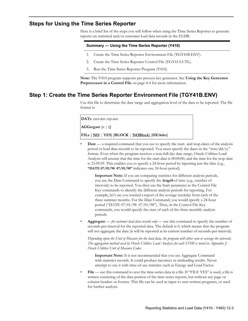
Steps for Using the Time Series ReporterHere is a brief list of the steps you will follow when using the Time Series Reporter to generate reports on statistical and/or customer load data records in the ELDB.
Note: The Y410 program supports pre-process key generator. See Using the Key Generator Preprocessor in a Control File on page 4-4 for more information.
Step 1: Create the Time Series Reporter Environment File (TGY41B.ENV)Use this file to determine the date range and aggregation level of the data to be reported. The file format is:
• Date — a required command that you use to specify the start- and stop-dates of the analysis period or load data records to be reported. You must specify the dates in the “mm/dd/yy” format. Even when the program receives a non-full-day date range, Oracle Utilities Load Analysis will assume that the time for the start-date is 00:00:00, and the time for the stop-date is 23:59:59. This enables you to specify a 24-hour period by inputting just the date (e.g., “DATE 07/01/98 07/01/98” indicates one 24-hour period).
Important Note: If you are comparing statistics for different analysis periods, you use the Date Command to specify the length of time (e.g., number of intervals) to be reported. You then use the Start parameter in the Control File Key commands to identify the different analysis periods for reporting. For example, let’s say you wanted a report of the average weekday from each of the three summer months. For the Date Command, you would specify a 24-hour period (“DATE 07/01/98 07/01/98”). Then, in the Control File Key commands, you would specify the start of each of the three monthly analysis periods.
• Aggregate — for customer load data records only — use this command to specify the number of seconds-per-interval for the reported data. The default is 0, which means that the program will not aggregate the data (it will be reported at its current number of seconds-per-interval).
Depending upon the Unit of Measure for the load data, the program will either sum or average the intervals. The aggregation method used by Oracle Utilities Load Analysis for each UOM is noted in Appendix J: Oracle Utilities Unit of Measure Codes.
Important Note: It is not recommended that you use Aggregate Command with statistics records. It could produce incorrect or misleading results. Never attempt to use it with time-of-use statistics such as Energy and Load Factor.
• File — use this command to save the time-series data in a file. If “FILE YES” is used, a file is written consisting of the data portion of the time-series reports, but without any page or column headers or footers. This file can be used as input to user-written programs, or used for further analysis.
Summary — Using the Time Series Reporter (Y410)
1. Create the Time Series Reporter Environment File (TGY41B.ENV).
2. Create the Time Series Reporter Control File (TGY41A.CTL).
3. Run the Time Series Reporter Program (Y410).
DATe start-date stop-date
AGGregate [n | 0]
FILe [ NO | YES] [BLOCK | NOBlock] [HEAder]
Reporting Statistics and Load Data (Y410 - Y460) 12-3
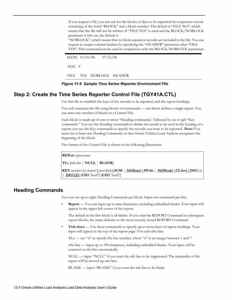
If you request a file, you can ask for the blocks of data to be separated by a separator record consisting of the word “BLOCK” and a block number. The default is “FILE NO”, which means that the file will not be written. If “FILE YES” is used and the BLOCK/NOBLOCK parameter is left out, the default is “NOBLOCK”, which means that no block separator records are included in the file. You can request to output column headers by specifying the “HEADER” parameter after “FILE YES”. This command can be used in conjunction with the BLOCK/NOBLOCK parameter.
Figure 11-9 Sample Time Series Reporter Environment File
Step 2: Create the Time Series Reporter Control File (TGY41A.CTL)Use this file to establish the keys of the records to be reported, and the report headings.
You will construct the file using blocks of commands — one block defines a single report. You can enter any number of blocks in a Control File.
Each block is made up of one or more “Heading commands,” followed by one to eight “Key commands.” You use the Heading commands to define the words to be used in the heading of a report; you use the Key commands to specify the records you want to be reported. Note: You must use at least one Heading Command, so that Oracle Utilities Load Analysis recognizes the beginning of the block.
The format of the Control File is shown in the following illustration.
Heading CommandsYou can use up to eight Heading Commands per block. Input one command per line.
• Report — You can input up to nine characters, including embedded blanks. Your input will appear in the upper left corner of the report.
The default in the first block is all blanks. If you omit the REPORT Command in subsequent report blocks, the name defaults to the most recently issued REPORT Command.
• Title-lines — Use these commands to specify up to seven lines of report headings. Your input will appear at the top of the report page. For each title-line:
TLn — use “n” to specify the line number, where “n” is an integer between 1 and 7.
title-line — input up to 190 characters, including embedded blanks. Your input will be centered on the line automatically.
NULL — input “NULL” if you want the nth line to be suppressed. The remainder of the report will be moved up one line.
BLANK — input “BLANK” if you want the nth line to be blank.
DATE 07/01/98 07/31/98
AGG 0
FILE YES NOBLOCK HEADER
REPort report-name
TLn [title-line | NULL | BLANK]
KEY customer-id, channel [,start-date] [,SUM | ,NOSum] [,PEAk | ,NOPeak] [,CLAss] [,DEC(n) | ,DEC(2)] [CH1 ‘head1’] [CH2 ‘head2’]
12-4 Oracle Utilities Load Analysis Load Data Analysis User’s Guide
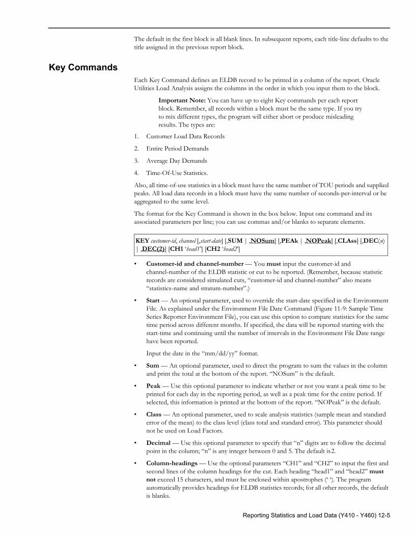
The default in the first block is all blank lines. In subsequent reports, each title-line defaults to the title assigned in the previous report block.
Key CommandsEach Key Command defines an ELDB record to be printed in a column of the report. Oracle Utilities Load Analysis assigns the columns in the order in which you input them to the block.
Important Note: You can have up to eight Key commands per each report block. Remember, all records within a block must be the same type. If you try to mix different types, the program will either abort or produce misleading results. The types are:
1. Customer Load Data Records
2. Entire Period Demands
3. Average Day Demands
4. Time-Of-Use Statistics.
Also, all time-of-use statistics in a block must have the same number of TOU periods and supplied peaks. All load data records in a block must have the same number of seconds-per-interval or be aggregated to the same level.
The format for the Key Command is shown in the box below. Input one command and its associated parameters per line; you can use commas and/or blanks to separate elements.
• Customer-id and channel-number — You must input the customer-id and channel-number of the ELDB statistic or cut to be reported. (Remember, because statistic records are considered simulated cuts, “customer-id and channel-number” also means “statistics-name and stratum-number”.)
• Start — An optional parameter, used to override the start-date specified in the Environment File. As explained under the Environment File Date Command (Figure 11-9: Sample Time Series Reporter Environment File), you can use this option to compare statistics for the same time period across different months. If specified, the data will be reported starting with the start-time and continuing until the number of intervals in the Environment File Date range have been reported.
Input the date in the “mm/dd/yy” format.
• Sum — An optional parameter, used to direct the program to sum the values in the column and print the total at the bottom of the report. “NOSum” is the default.
• Peak — Use this optional parameter to indicate whether or not you want a peak time to be printed for each day in the reporting period, as well as a peak time for the entire period. If selected, this information is printed at the bottom of the report. “NOPeak” is the default.
• Class — An optional parameter, used to scale analysis statistics (sample mean and standard error of the mean) to the class level (class total and standard error). This parameter should not be used on Load Factors.
• Decimal — Use this optional parameter to specify that “n” digits are to follow the decimal point in the column; “n” is any integer between 0 and 5. The default is2.
• Column-headings — Use the optional parameters “CH1” and “CH2” to input the first and second lines of the column headings for the cut. Each heading “head1” and “head2” must not exceed 15 characters, and must be enclosed within apostrophes (‘ ‘). The program automatically provides headings for ELDB statistics records; for all other records, the default is blanks.
KEY customer-id, channel [,start-date] [,SUM | ,NOSum] [,PEAk | ,NOPeak] [,CLAss] [,DEC(n) | ,DEC(2)] [CH1 ‘head1’] [CH2 ‘head2’]
Reporting Statistics and Load Data (Y410 - Y460) 12-5
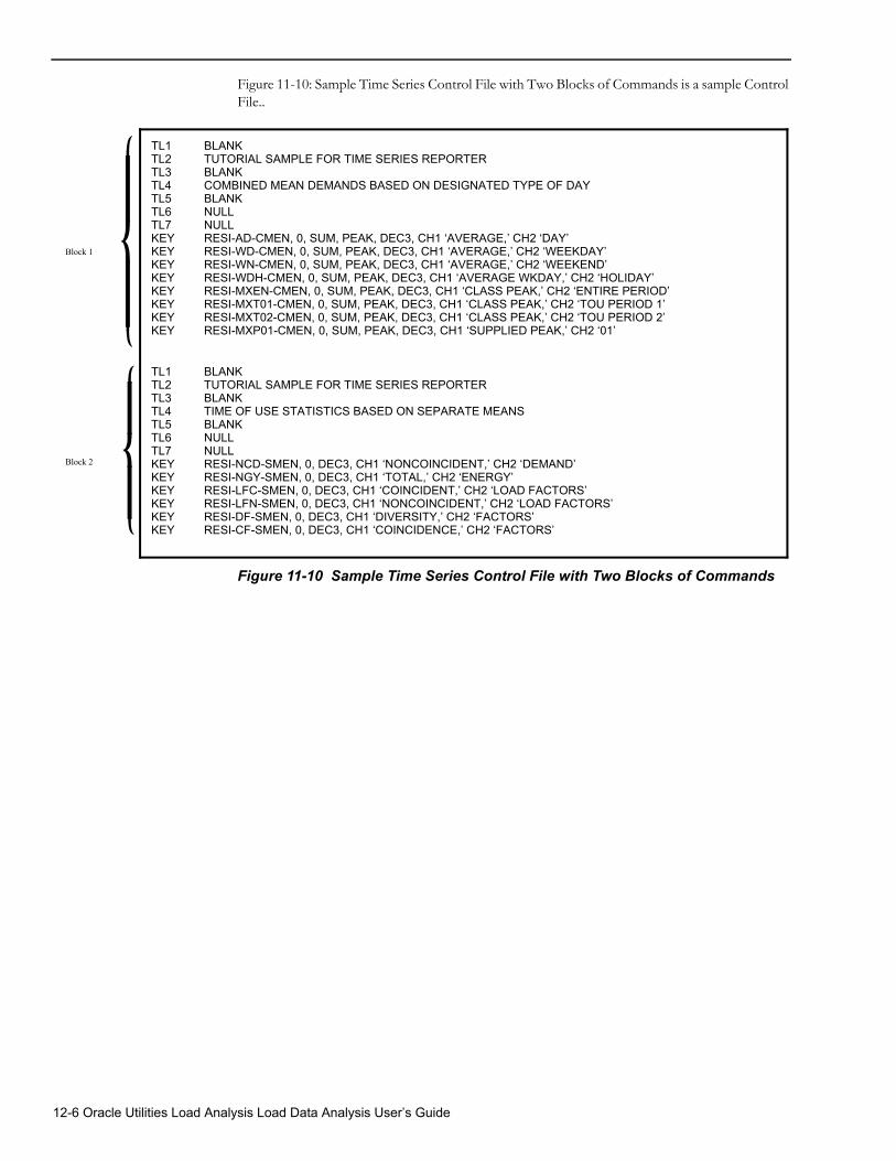
Figure 11-10: Sample Time Series Control File with Two Blocks of Commands is a sample Control File..
Figure 11-10 Sample Time Series Control File with Two Blocks of Commands
TL1 BLANKTL2 TUTORIAL SAMPLE FOR TIME SERIES REPORTERTL3 BLANKTL4 COMBINED MEAN DEMANDS BASED ON DESIGNATED TYPE OF DAYTL5 BLANKTL6 NULLTL7 NULLKEY RESI-AD-CMEN, 0, SUM, PEAK, DEC3, CH1 ‘AVERAGE,’ CH2 ‘DAY’KEY RESI-WD-CMEN, 0, SUM, PEAK, DEC3, CH1 ‘AVERAGE,’ CH2 ‘WEEKDAY’KEY RESI-WN-CMEN, 0, SUM, PEAK, DEC3, CH1 ‘AVERAGE,’ CH2 ‘WEEKEND’KEY RESI-WDH-CMEN, 0, SUM, PEAK, DEC3, CH1 ‘AVERAGE WKDAY,’ CH2 ‘HOLIDAY’KEY RESI-MXEN-CMEN, 0, SUM, PEAK, DEC3, CH1 ‘CLASS PEAK,’ CH2 ‘ENTIRE PERIOD’KEY RESI-MXT01-CMEN, 0, SUM, PEAK, DEC3, CH1 ‘CLASS PEAK,’ CH2 ‘TOU PERIOD 1’KEY RESI-MXT02-CMEN, 0, SUM, PEAK, DEC3, CH1 ‘CLASS PEAK,’ CH2 ‘TOU PERIOD 2’KEY RESI-MXP01-CMEN, 0, SUM, PEAK, DEC3, CH1 ‘SUPPLIED PEAK,’ CH2 ‘01’
TL1 BLANKTL2 TUTORIAL SAMPLE FOR TIME SERIES REPORTERTL3 BLANKTL4 TIME OF USE STATISTICS BASED ON SEPARATE MEANSTL5 BLANKTL6 NULLTL7 NULLKEY RESI-NCD-SMEN, 0, DEC3, CH1 ‘NONCOINCIDENT,’ CH2 ‘DEMAND’KEY RESI-NGY-SMEN, 0, DEC3, CH1 ‘TOTAL,’ CH2 ‘ENERGY’KEY RESI-LFC-SMEN, 0, DEC3, CH1 ‘COINCIDENT,’ CH2 ‘LOAD FACTORS’KEY RESI-LFN-SMEN, 0, DEC3, CH1 ‘NONCOINCIDENT,’ CH2 ‘LOAD FACTORS’KEY RESI-DF-SMEN, 0, DEC3, CH1 ‘DIVERSITY,’ CH2 ‘FACTORS’KEY RESI-CF-SMEN, 0, DEC3, CH1 ‘COINCIDENCE,’ CH2 ‘FACTORS’
Block 1
Block 2
12-6 Oracle Utilities Load Analysis Load Data Analysis User’s Guide
Step 3: Run the Time Series Reporter Program (Y410)Once you have created the Environment and Control Files, you are ready to run the Time Series Reporter. Use Y410.
Time Series Reporting ProcessingFor each report block of Heading and Key commands, the program sets up the page and column headings, locates each cut in the ELDB, and prints the data. If supplied peak and/or time-of-use statistics are being reported, an appropriate label is placed in the first column of the report for each row of data. Otherwise, the first column in the report specifies the time of day for the corresponding row of data. The data is printed in the seconds-per-interval units specified in the AGGREGATE Command. All ELDB cuts specified in a report block must have the same seconds-per-interval attribute, or be aggregated to the same level. If the SUM parameter is specified in a KEY Command, the sum of the values in the column is calculated and printed at the bottom of the column for each day of the report. When the SUM option is specified for demand data (i.e., data with a unit-of-measure code of 02), the total reported represents summed energy values. Similarly, if the PEAK parameter of the KEY Command is in effect, the time of day when the peak occurs is printed for each day in the reporting period. In addition, the time of the peak over the entire period is printed at the end of the report. Illegal Heading commands will cause the program to terminate; illegal Key commands are merely ignored. All illegal commands and missing cuts are reported in an Error Log.
Load Data Reporter (Y420, Y430)The Load Data Reporter produces detailed reports on individual statistics or customer load data records in the ELDB or SLDB. For load data records, you can report a cut, a cut series, or subsetted portions of cut series. You would typically use this program to investigate load data cuts before editing, or to look at the detailed information contained in a statistics record that is not shown in the analysis reports, such as population and weight.
The Reporter is very flexible and gives you many options for printing detailed information on customers or statistics records:
• Load Data Report — Includes descriptive information such as time span, minutes per interval, and unit of measure for customer load data records; or length of analysis period, population, and weight for statistics records.
• Data Dump Report — “Dumps” of interval data — i.e., a complete list of every interval in the record. For load data records, you can specify interval data in two formats:
• energy dumps — pulse data multiplied by the pulse multiplier and added to the pulse offset
• demand dumps — energy values multiplied by the number of recording intervals per hour.
For statistics records, use only the Energy dump report — the demand dump will produce misleading or erroneous data.
• Summary Report — Summaries of peak minimum or daily data. You can request three types of summary report:
• peak summary — The ten highest energy values in the cut, series, or subset, showing the value and time.
• minimum summary — The ten lowest energy values in the cut, series, or subset, showing the time.
• daily energy, peak and minimum — Total energy peak and minimum values for each day in the cut, series, or subset.
Reporting Statistics and Load Data (Y410 - Y460) 12-7
Samples of these reports are shown at the end of this section.
Steps for Using the Load Data Reporter
Step 1: Identify Records to be Reported and Type of Report Needed for Each One
The flexibility of the Reporter enables you to quickly generate reports for a group of records in a single session. The report type can be the same for all records, or specially modified for each one.
Step 2: Create Environment File (TGX41B.ENV)You define the contents and format of the reports using a combination of the Environment File and the Control File (Figure 11-16: Constructing Load Data Reports). In general, use the Environment File to define the basic report (in other words, the report structure you will want most often). Use the Control File to specify the records to be reported, and any modifications of reports required for specific records.
Special Note about Using the Load Data Reporter for Statistics
Follow the same steps when using the Load Data Reporter for either statistics or customer load data records. However, there are some important points to keep in mind when using the program to report statistical records:1. Use the Reporter only for interval demands, not time-of-use statistics.
2. Report interval statistics using the Energy option, never the Demand option.
3. Never attempt to aggregate statistics.
4. Statistics will be printed in the customer load data report format. This means that, although the field identifiers appear the same on both types of records, they will have different meanings. These differences are thoroughly explained in Header and Interval Data for Statistics Records on page 3-10.
Summary—Using the Load Data Reporter (Y420, Y430)
1. Identify records to be reported and determine type of report needed for each one.
2. Create Environment File (TGX41B.ENV).
3. Create Control File (TGX41A.CTL).
4. Run Load Data Reporter (Y420 for ELDB, Y430 for SLDB).
12-8 Oracle Utilities Load Analysis Load Data Analysis User’s Guide
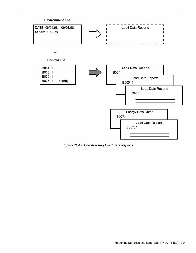
Figure 11-16 Constructing Load Data Reports
Load Data ReportsB004, 1
Load Data ReportsB005, 1
Load Data ReportsB006, 1
Energy Data DumpB007, 1
Load Data ReportsB007, 1
Load Data Reports
Environment File
DATE 06/01/98 09/01/98SOURCE ELDB
Control File
+
B004, 1B005, 1B006, 1B007, 1 Energy
Reporting Statistics and Load Data (Y410 - Y460) 12-9
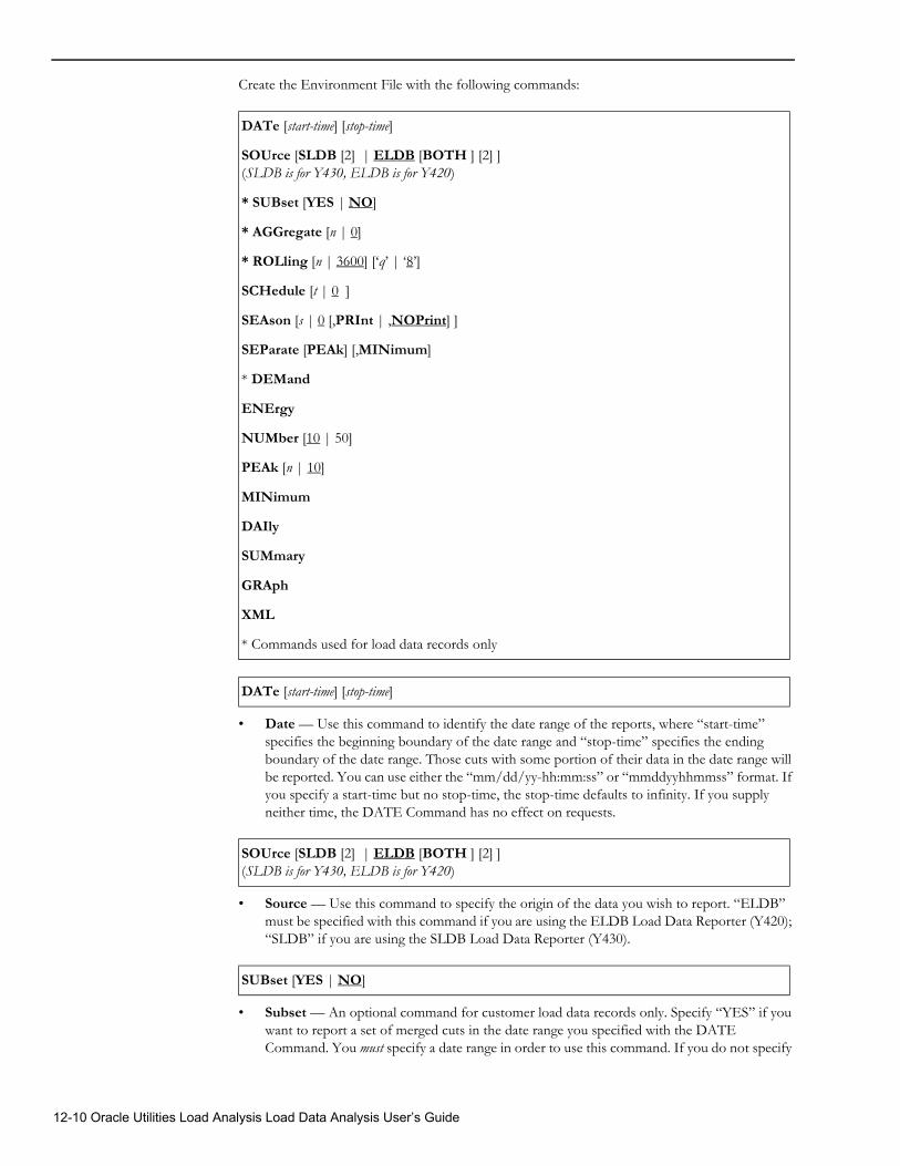
Create the Environment File with the following commands:
• Date — Use this command to identify the date range of the reports, where “start-time” specifies the beginning boundary of the date range and “stop-time” specifies the ending boundary of the date range. Those cuts with some portion of their data in the date range will be reported. You can use either the “mm/dd/yy-hh:mm:ss” or “mmddyyhhmmss” format. If you specify a start-time but no stop-time, the stop-time defaults to infinity. If you supply neither time, the DATE Command has no effect on requests.
• Source — Use this command to specify the origin of the data you wish to report. “ELDB” must be specified with this command if you are using the ELDB Load Data Reporter (Y420); “SLDB” if you are using the SLDB Load Data Reporter (Y430).
• Subset — An optional command for customer load data records only. Specify “YES” if you want to report a set of merged cuts in the date range you specified with the DATE Command. You must specify a date range in order to use this command. If you do not specify
DATe [start-time] [stop-time]
SOUrce [SLDB [2] | ELDB [BOTH ] [2] ] (SLDB is for Y430, ELDB is for Y420)
* SUBset [YES | NO]
* AGGregate [n | 0]
* ROLling [n | 3600] [‘q’ | ‘8’]
SCHedule [t | 0 ]
SEAson [s | 0 [,PRInt | ,NOPrint] ]
SEParate [PEAk] [,MINimum]
* DEMand
ENErgy
NUMber [10 | 50]
PEAk [n | 10]
MINimum
DAIly
SUMmary
GRAph
XML
* Commands used for load data records only
DATe [start-time] [stop-time]
SOUrce [SLDB [2] | ELDB [BOTH ] [2] ] (SLDB is for Y430, ELDB is for Y420)
SUBset [YES | NO]
12-10 Oracle Utilities Load Analysis Load Data Analysis User’s Guide
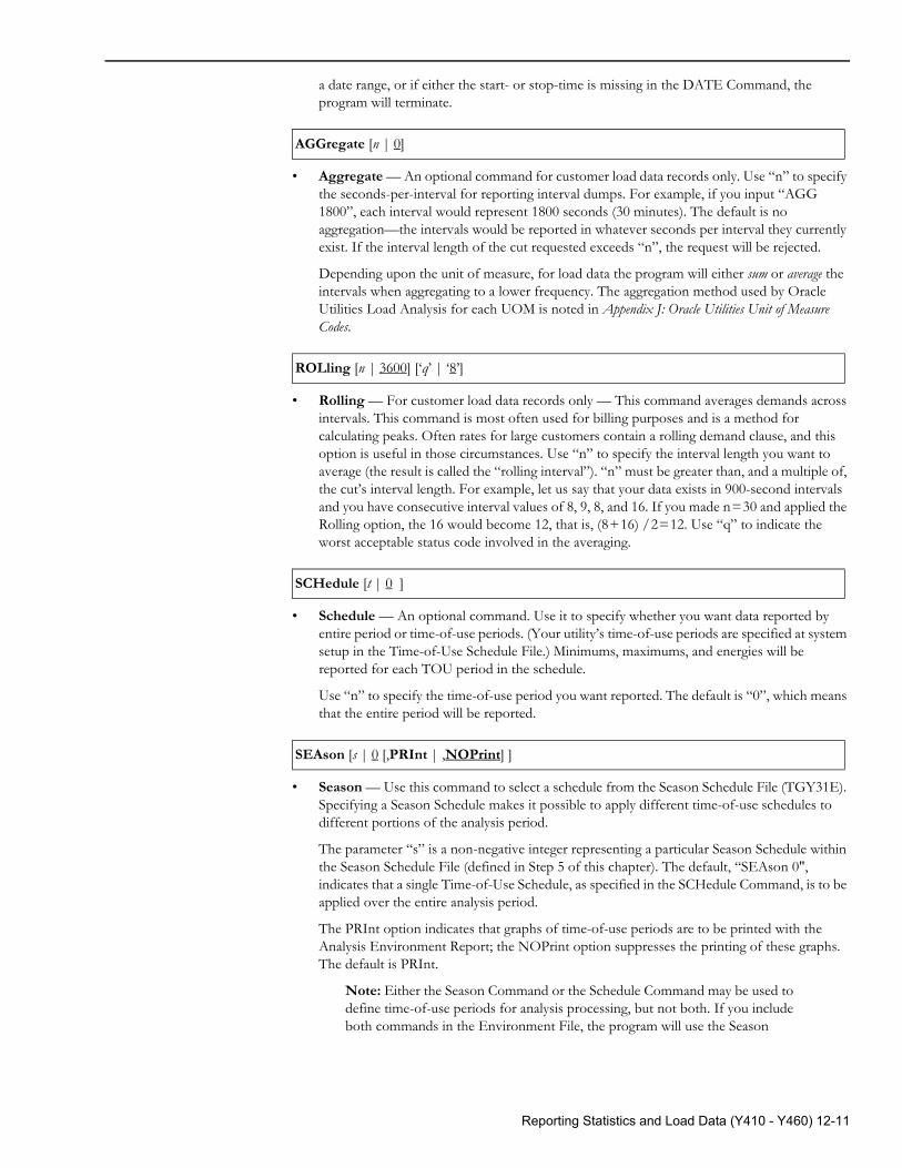
a date range, or if either the start- or stop-time is missing in the DATE Command, the program will terminate.
• Aggregate — An optional command for customer load data records only. Use “n” to specify the seconds-per-interval for reporting interval dumps. For example, if you input “AGG 1800”, each interval would represent 1800 seconds (30 minutes). The default is no aggregation—the intervals would be reported in whatever seconds per interval they currently exist. If the interval length of the cut requested exceeds “n”, the request will be rejected.
Depending upon the unit of measure, for load data the program will either sum or average the intervals when aggregating to a lower frequency. The aggregation method used by Oracle Utilities Load Analysis for each UOM is noted in Appendix J: Oracle Utilities Unit of Measure Codes.
• Rolling — For customer load data records only — This command averages demands across intervals. This command is most often used for billing purposes and is a method for calculating peaks. Often rates for large customers contain a rolling demand clause, and this option is useful in those circumstances. Use “n” to specify the interval length you want to average (the result is called the “rolling interval”). “n” must be greater than, and a multiple of, the cut’s interval length. For example, let us say that your data exists in 900-second intervals and you have consecutive interval values of 8, 9, 8, and 16. If you made n=30 and applied the Rolling option, the 16 would become 12, that is, (8+16) /2=12. Use “q” to indicate the worst acceptable status code involved in the averaging.
• Schedule — An optional command. Use it to specify whether you want data reported by entire period or time-of-use periods. (Your utility’s time-of-use periods are specified at system setup in the Time-of-Use Schedule File.) Minimums, maximums, and energies will be reported for each TOU period in the schedule.
Use “n” to specify the time-of-use period you want reported. The default is “0”, which means that the entire period will be reported.
• Season — Use this command to select a schedule from the Season Schedule File (TGY31E). Specifying a Season Schedule makes it possible to apply different time-of-use schedules to different portions of the analysis period.
The parameter “s” is a non-negative integer representing a particular Season Schedule within the Season Schedule File (defined in Step 5 of this chapter). The default, “SEAson 0", indicates that a single Time-of-Use Schedule, as specified in the SCHedule Command, is to be applied over the entire analysis period.
The PRInt option indicates that graphs of time-of-use periods are to be printed with the Analysis Environment Report; the NOPrint option suppresses the printing of these graphs. The default is PRInt.
Note: Either the Season Command or the Schedule Command may be used to define time-of-use periods for analysis processing, but not both. If you include both commands in the Environment File, the program will use the Season
AGGregate [n | 0]
ROLling [n | 3600] [‘q’ | ‘8’]
SCHedule [t | 0 ]
SEAson [s | 0 [,PRInt | ,NOPrint] ]
Reporting Statistics and Load Data (Y410 - Y460) 12-11
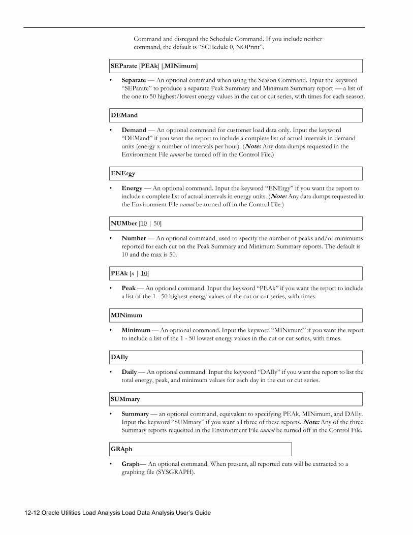
Command and disregard the Schedule Command. If you include neither command, the default is “SCHedule 0, NOPrint”.
• Separate — An optional command when using the Season Command. Input the keyword “SEParate” to produce a separate Peak Summary and Minimum Summary report — a list of the one to 50 highest/lowest energy values in the cut or cut series, with times for each season.
• Demand — An optional command for customer load data only. Input the keyword “DEMand” if you want the report to include a complete list of actual intervals in demand units (energy x number of intervals per hour). (Note: Any data dumps requested in the Environment File cannot be turned off in the Control File.)
• Energy — An optional command. Input the keyword “ENErgy” if you want the report to include a complete list of actual intervals in energy units. (Note: Any data dumps requested in the Environment File cannot be turned off in the Control File.)
• Number — An optional command, used to specify the number of peaks and/or minimums reported for each cut on the Peak Summary and Minimum Summary reports. The default is 10 and the max is 50.
• Peak — An optional command. Input the keyword “PEAk” if you want the report to include a list of the 1 - 50 highest energy values of the cut or cut series, with times.
• Minimum — An optional command. Input the keyword “MINimum” if you want the report to include a list of the 1 - 50 lowest energy values in the cut or cut series, with times.
• Daily — An optional command. Input the keyword “DAIly” if you want the report to list the total energy, peak, and minimum values for each day in the cut or cut series.
• Summary — an optional command, equivalent to specifying PEAk, MINimum, and DAIly. Input the keyword “SUMmary” if you want all three of these reports. Note: Any of the three Summary reports requested in the Environment File cannot be turned off in the Control File.
• Graph— An optional command. When present, all reported cuts will be extracted to a graphing file (SYSGRAPH).
SEParate [PEAk] [,MINimum]
DEMand
ENErgy
NUMber [10 | 50]
PEAk [n | 10]
MINimum
DAIly
SUMmary
GRAph
12-12 Oracle Utilities Load Analysis Load Data Analysis User’s Guide
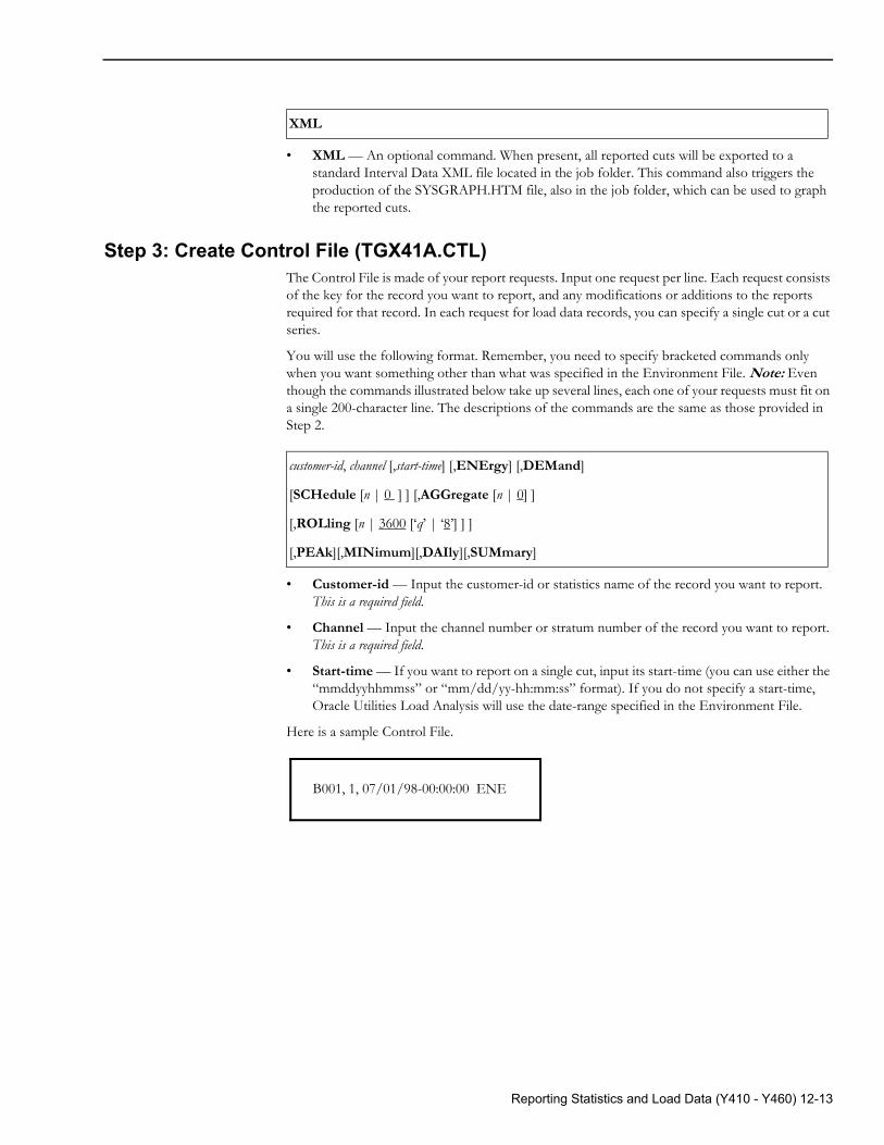
• XML — An optional command. When present, all reported cuts will be exported to a standard Interval Data XML file located in the job folder. This command also triggers the production of the SYSGRAPH.HTM file, also in the job folder, which can be used to graph the reported cuts.
Step 3: Create Control File (TGX41A.CTL)The Control File is made of your report requests. Input one request per line. Each request consists of the key for the record you want to report, and any modifications or additions to the reports required for that record. In each request for load data records, you can specify a single cut or a cut series.
You will use the following format. Remember, you need to specify bracketed commands only when you want something other than what was specified in the Environment File. Note: Even though the commands illustrated below take up several lines, each one of your requests must fit on a single 200-character line. The descriptions of the commands are the same as those provided in Step 2.
• Customer-id — Input the customer-id or statistics name of the record you want to report. This is a required field.
• Channel — Input the channel number or stratum number of the record you want to report. This is a required field.
• Start-time — If you want to report on a single cut, input its start-time (you can use either the “mmddyyhhmmss” or “mm/dd/yy-hh:mm:ss” format). If you do not specify a start-time, Oracle Utilities Load Analysis will use the date-range specified in the Environment File.
Here is a sample Control File.
XML
customer-id, channel [,start-time] [,ENErgy] [,DEMand]
[SCHedule [n | 0 ] ] [,AGGregate [n | 0] ]
[,ROLling [n | 3600 [‘q’ | ‘8’] ] ]
[,PEAk][,MINimum][,DAIly][,SUMmary]
B001, 1, 07/01/98-00:00:00 ENE
Reporting Statistics and Load Data (Y410 - Y460) 12-13
Step 4: Run the Load Data Reporter (Y420 or Y430)Once you have created the Environment File and the Control File you are ready to run the Load Data Reporter. Use Y420 for the ELDB or Y430 for the SLDB.
Load Data Reporter ProcessingThe Load Data Reporter Program checks the Environment File to determine what options have been chosen and if they are consistent. The following conditions halt processing.
• Subset mode specified without a date range or with an incomplete date range (i.e., a start-time and no stop-time)
• An invalid aggregation level (i.e., a level that is lower than the data’s original level of aggregation)
• An invalid rolling level of aggregation (same as aggregation problem above)
• A rolling level of aggregation equal to the data’s original level of aggregation
• Subset specified and cuts not eligible for merge.
Each key in the Control File is processed by finding a corresponding cut or cut series in the ELDB or SLDB. When a date range is specified in the Environment File, if the start-time of the request key (if stated) is not within the date range, an error message is produced and processing continues with the next key in the Control File. If subset is set to “YES”, one report is generated that includes data from one cut (if the request key is a full key), or from a cut series whose data falls within the date range specified. If subset is set to “NO”, a report for each cut that has data within the date range is generated, or one report is produced for a full key request. WARNING: When data is aggregated, the original start- and stop-times of the ELDB or SLDB cut are used for comparison with the date range. A stop-time of the reported cut is calculated using the number of recorded intervals, and may differ from the original cut stop-time if data is missing.
If date range is set to “ALL”, data for all cuts in the ELDB or SLDB with the same customer-id and channel as the request key is selected, and a descriptive report is generated for each cut. If the request key is a full key, one report on one cut is produced.
If aggregation and/or subsetting are requested, the stop-time, recorded and expected intervals, and total energy of the reported cut are calculated from information from an ELDB or SLDB cut or cuts; meter data is set to zero. Printing of the validation messages is suppressed because these messages do not apply to the synthesized cuts reported. If at least one of the options “Energy” or “Demand” are specified, an interval data report(s), a Peak Summary Report(s), a Minimum Summary Report(s), and a Daily Energy, Peak and Minimum Report(s) will follow the descriptive data report. WARNING: If ROLling is specified, and if the status code of each interval is less than or equal to the worst acceptable status code stated in the Environment File, the interval is not included in the average.
If the SCHEDULE Command is included in the Environment File, then all cuts will have the Peak Summary, Minimum Summary, and Daily Energy, Peak and Minimum reports as part of their output. If a schedule number other than zero is chosen, these reports will be broken down by the time-of-use period associated with that schedule number. If the “PRInt” option is chosen, time-of-use period graphs will be printed as part of the output; otherwise, these are omitted.
12-14 Oracle Utilities Load Analysis Load Data Analysis User’s Guide
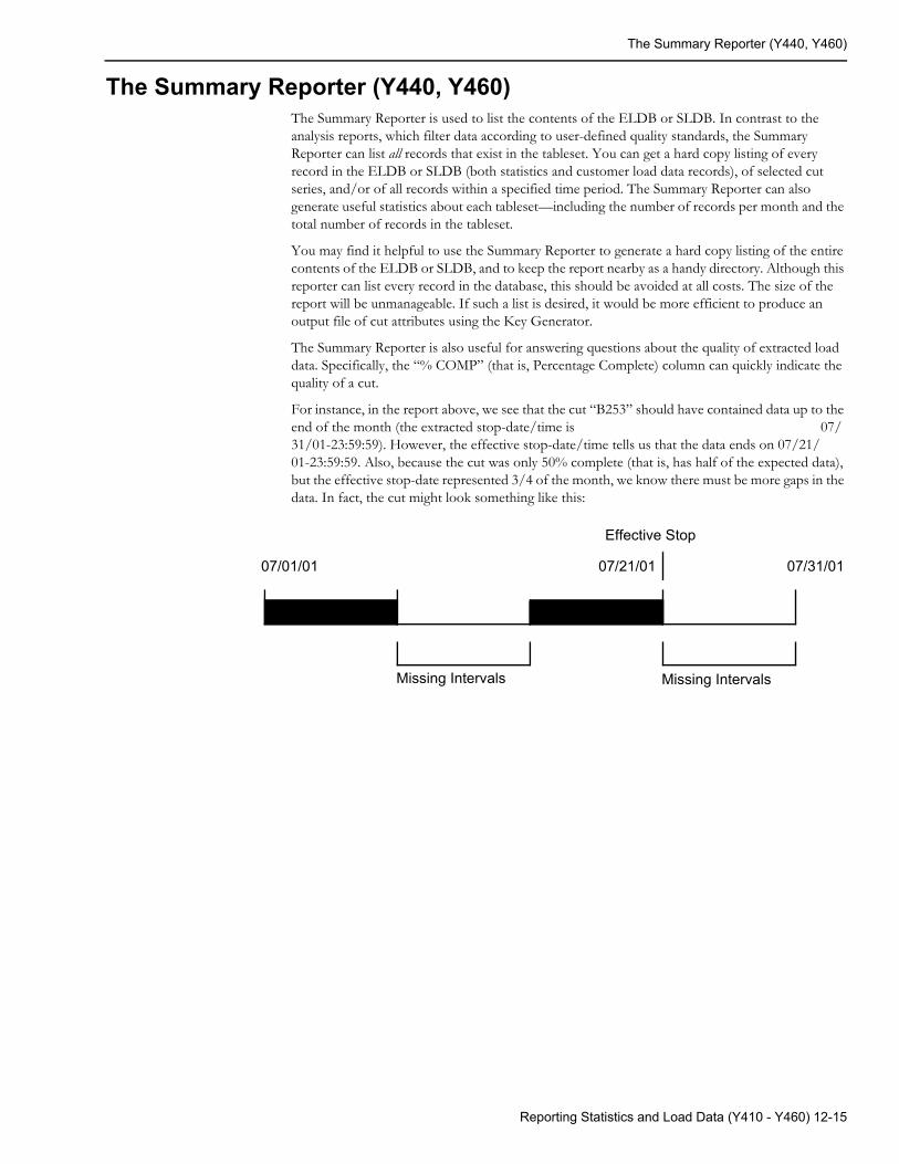
The Summary Reporter (Y440, Y460)
The Summary Reporter (Y440, Y460)The Summary Reporter is used to list the contents of the ELDB or SLDB. In contrast to the analysis reports, which filter data according to user-defined quality standards, the Summary Reporter can list all records that exist in the tableset. You can get a hard copy listing of every record in the ELDB or SLDB (both statistics and customer load data records), of selected cut series, and/or of all records within a specified time period. The Summary Reporter can also generate useful statistics about each tableset—including the number of records per month and the total number of records in the tableset.
You may find it helpful to use the Summary Reporter to generate a hard copy listing of the entire contents of the ELDB or SLDB, and to keep the report nearby as a handy directory. Although this reporter can list every record in the database, this should be avoided at all costs. The size of the report will be unmanageable. If such a list is desired, it would be more efficient to produce an output file of cut attributes using the Key Generator.
The Summary Reporter is also useful for answering questions about the quality of extracted load data. Specifically, the “% COMP” (that is, Percentage Complete) column can quickly indicate the quality of a cut.
For instance, in the report above, we see that the cut “B253” should have contained data up to the end of the month (the extracted stop-date/time is 07/31/01-23:59:59). However, the effective stop-date/time tells us that the data ends on 07/21/01-23:59:59. Also, because the cut was only 50% complete (that is, has half of the expected data), but the effective stop-date represented 3/4 of the month, we know there must be more gaps in the data. In fact, the cut might look something like this:
07/01/01 07/21/01 07/31/01
Missing Intervals Missing Intervals
Effective Stop
Reporting Statistics and Load Data (Y410 - Y460) 12-15
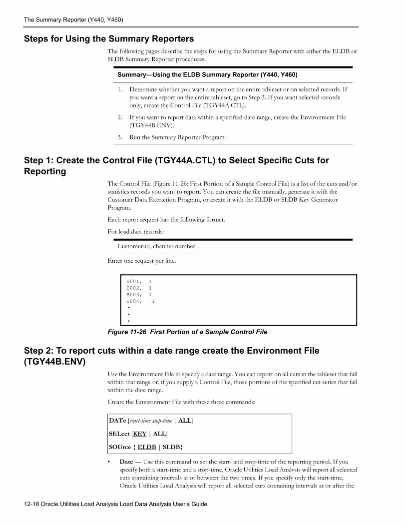
The Summary Reporter (Y440, Y460)
Steps for Using the Summary ReportersThe following pages describe the steps for using the Summary Reporter with either the ELDB or SLDB Summary Reporter procedures.
Step 1: Create the Control File (TGY44A.CTL) to Select Specific Cuts for Reporting
The Control File (Figure 11-26: First Portion of a Sample Control File) is a list of the cuts and/or statistics records you want to report. You can create the file manually, generate it with the Customer Data Extraction Program, or create it with the ELDB or SLDB Key Generator Program.
Each report request has the following format.
For load data records:
Enter one request per line.
Figure 11-26 First Portion of a Sample Control File
Step 2: To report cuts within a date range create the Environment File (TGY44B.ENV)
Use the Environment File to specify a date range. You can report on all cuts in the tableset that fall within that range or, if you supply a Control File, those portions of the specified cut series that fall within the date range.
Create the Environment File with these three commands:
• Date — Use this command to set the start- and stop-time of the reporting period. If you specify both a start-time and a stop-time, Oracle Utilities Load Analysis will report all selected cuts containing intervals at or between the two times. If you specify only the start-time, Oracle Utilities Load Analysis will report all selected cuts containing intervals at or after the
Summary—Using the ELDB Summary Reporter (Y440, Y460)
1. Determine whether you want a report on the entire tableset or on selected records. If you want a report on the entire tableset, go to Step 3. If you want selected records only, create the Control File (TGY44A.CTL).
2. If you want to report data within a specified date range, create the Environment File (TGY44B.ENV).
3. Run the Summary Reporter Program .
Customer-id, channel-number
B001, 1B002, 1B003, 1B004, 1•••
DATe [start-time stop-time | ALL]
SELect [KEY | ALL]
SOUrce { ELDB | SLDB}
12-16 Oracle Utilities Load Analysis Load Data Analysis User’s Guide
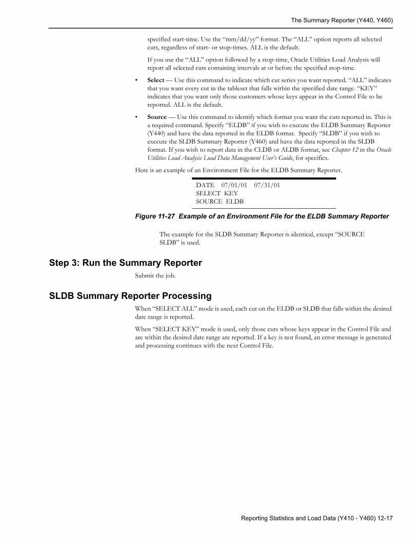
The Summary Reporter (Y440, Y460)
specified start-time. Use the “mm/dd/yy” format. The “ALL” option reports all selected cuts, regardless of start- or stop-times. ALL is the default.
If you use the “ALL” option followed by a stop-time, Oracle Utilities Load Analysis will report all selected cuts containing intervals at or before the specified stop-time.
• Select — Use this command to indicate which cut series you want reported. “ALL” indicates that you want every cut in the tableset that falls within the specified date range. “KEY” indicates that you want only those customers whose keys appear in the Control File to be reported. ALL is the default.
• Source — Use this command to identify which format you want the cuts reported in. This is a required command. Specify “ELDB” if you wish to execute the ELDB Summary Reporter (Y440) and have the data reported in the ELDB format. Specify “SLDB” if you wish to execute the SLDB Summary Reporter (Y460) and have the data reported in the SLDB format. If you wish to report data in the CLDB or ALDB format, see Chapter 12 in the Oracle Utilities Load Analysis Load Data Management User’s Guide, for specifics.
Here is an example of an Environment File for the ELDB Summary Reporter.
Figure 11-27 Example of an Environment File for the ELDB Summary Reporter
The example for the SLDB Summary Reporter is identical, except “SOURCE SLDB” is used.
Step 3: Run the Summary ReporterSubmit the job.
SLDB Summary Reporter ProcessingWhen “SELECT ALL” mode is used, each cut on the ELDB or SLDB that falls within the desired date range is reported.
When “SELECT KEY” mode is used, only those cuts whose keys appear in the Control File and are within the desired date range are reported. If a key is not found, an error message is generated and processing continues with the next Control File.
DATE 07/01/01 07/31/01SELECT KEYSOURCE ELDB
Reporting Statistics and Load Data (Y410 - Y460) 12-17

The Summary Reporter (Y440, Y460)
12-18 Oracle Utilities Load Analysis Load Data Analysis User’s Guide

Chapter 13Computing Customer Energy Use by Billing
Cycles Using the Billed Energy Program (Y230)
It is frequently necessary to analyze customer energy use on a billing cycle basis — for ratio expansions, for a company energy sale study, or for other tasks. However, accurate values for individual customer use for monthly billing cycles may not be readily available. The information may be too difficult to extract from “Billing,” or it simply may not exist for all customers in an analysis.
This chapter explains how to use the Billed Energy Program to compute customer energy usage on a billing cycle basis from interval demand data that is available in a Oracle Utilities Load Analysis tableset.
Topics included in this chapter are:
• Why Accurate Energy for Billing Periods Is Important to Ratio Analysis
• What Does the Billed Energy Program Do?
• Steps for Using the Billed Energy Program (Y230)
Computing Customer Energy Use by Billing Cycles Using the Billed Energy Program (Y230) 13-1

Why Accurate Energy for Billing Periods Is Important to Ratio Analysis
Why Accurate Energy for Billing Periods Is Important to Ratio Analysis
Oracle Utilities Load Analysis’s Ratio Analysis, Domains Ratio, and Coincident Peak Analysis programs utilize the ratio expansion methodology to estimate class totals from sample customer data. The ratio of demand to billed energy for each interval, expanded by the sum of class bills, is used to obtain class total demand estimates.
Ratio expansion depends on accurate billed energy values for each customer in the sample, for the same periods over which the class bills were totaled. However, this information is often difficult to obtain from Billing.
One way to get the information is to direct the Oracle Utilities Load Analysis Analysis program to derive customer energy values from interval demand data in the Oracle Utilities Load Analysis tableset. This approach is not entirely satisfactory, however. The Analysis program computes energy values for all customers over the same date range, but the population is actually divided into groups whose monthly billing cycles begin on different days of the month. Thus the computed values for the sample customers do not accurately reflect the variety of date ranges over which the population billed energy was recorded.
This chapter explains how to use the Billed Energy Program to overcome this problem — that is, how to compute energy usage for customers on a billing cycle basis using interval demand data that is available in the Oracle Utilities Load Analysis tableset. The program also produces an output file formatted for use as the Control File for Analysis programs.
What Does the Billed Energy Program Do?The Billed Energy Program is designed to read interval data from the Oracle Utilities Load Analysis tableset and compute total energy between an arbitrary date range for specified customers. It may be used on the CLDB or ELDB, but does require valid records. The data may be of any time frequency, and may be spread across any number of cuts.
You specify a list of customers and their individual billing cycle numbers, along with a file that defines the start- and stop-date of each cycle. You may also specify blocks of customers whose records are to be accumulated and written back to the tableset as a single combined cut. The program automatically finds all interval data for each customer cycle that meets or exceeds a user-defined quality standard, prorates the data to adjust for missing or excluded intervals (if desired), and computes the total or billed energy. The program outputs a series of diagnostic reports, and a file that you can use as input to the Standard, Ratio, Domains, 100% Sample, or Coincident Peak Analysis programs, or to a custom external application. If block processing is performed, the program writes the combined cut(s) to the tableset; and in such a case information for the combined cut, rather than any of the block of cuts used to create it, is written to the output file. You may therefore find the program useful for accumulating cuts from different recorders and creating Control File records in preparation for running one of the above-mentioned Analysis programs, whether or not you not wish to calculate their billed energy.
13-2 Oracle Utilities Load Analysis Load Data Analysis User’s Guide
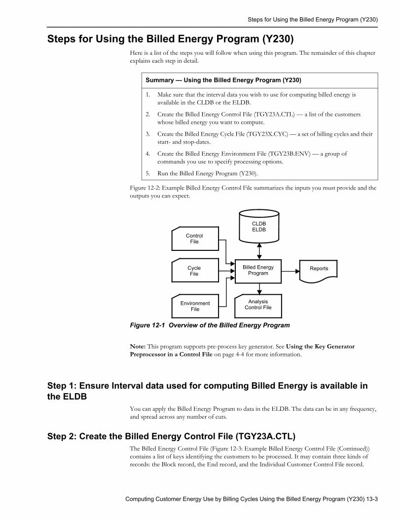
Steps for Using the Billed Energy Program (Y230)
Steps for Using the Billed Energy Program (Y230)Here is a list of the steps you will follow when using this program. The remainder of this chapter explains each step in detail.
Figure 12-2: Example Billed Energy Control File summarizes the inputs you must provide and the outputs you can expect.
Figure 12-1 Overview of the Billed Energy Program
Note: This program supports pre-process key generator. See Using the Key Generator Preprocessor in a Control File on page 4-4 for more information.
Step 1: Ensure Interval data used for computing Billed Energy is available in the ELDB
You can apply the Billed Energy Program to data in the ELDB. The data can be in any frequency, and spread across any number of cuts.
Step 2: Create the Billed Energy Control File (TGY23A.CTL)The Billed Energy Control File (Figure 12-3: Example Billed Energy Control File (Continued)) contains a list of keys identifying the customers to be processed. It may contain three kinds of records: the Block record, the End record, and the Individual Customer Control File record.
Summary — Using the Billed Energy Program (Y230)
1. Make sure that the interval data you wish to use for computing billed energy is available in the CLDB or the ELDB.
2. Create the Billed Energy Control File (TGY23A.CTL) — a list of the customers whose billed energy you want to compute.
3. Create the Billed Energy Cycle File (TGY23X.CYC) — a set of billing cycles and their start- and stop-dates.
4. Create the Billed Energy Environment File (TGY23B.ENV) — a group of commands you use to specify processing options.
5. Run the Billed Energy Program (Y230).
ControlFile
CycleFile
EnvironmentFile
Billed EnergyProgram
AnalysisControl File
Reports
CLDBELDB
Computing Customer Energy Use by Billing Cycles Using the Billed Energy Program (Y230) 13-3

Steps for Using the Billed Energy Program (Y230)
The Individual Customer record may have one of four formats, depending on the Analysis Type specified in the Environment File; the default is Ratio/Coincident Peak Analysis. You must provide one record for each customer, using one of the formats in the boxes below. There is no limit to the number of records in a file, and customer-ids may be repeated with different cycle numbers. Within the file, Individual Customer records can be placed in any order, except where constrained by Block and End records. Within a record, the parameters must be provided in the order shown. Parameters may be separated by blanks or by a comma. The “+ or -” parameter shown at the beginning of each format is valid only on records within an accumulation block, i.e., entered between a Block and an End record. On such records within a block, the parameters following channel-number are ignored, and may therefore be omitted.
Because billed energy is not input to the Standard, Domains Mean-per-Unit, and 100% Sample Analysis programs, it is not calculated by the Billed Energy Program for these Analysis Types, and therefore no cycle-number is required on their Control File records. For the other Analysis Types (Ratio/Coincident Peak and Domains Ratio), billed energy is calculated unless you specify the NOCALCULATE parameter on the TYPE Environment File Command. In that case, cycle-number may be omitted from these Control File records also; otherwise, it is required.
Standard Analysis Control File Record Format (Individual Customer)[ + ] customer-id, channel-number [ { + } chan1 [ { + } chan2...] ], stratum-number [, cycle-number]
Ratio or Coincident Peak Analysis Control File Record Format (Individual Customer)[ + ] customer-id, channel-number [ { + } chan1 [ { + } chan2...] ], stratum-number [, cycle-number]
Domains Mean-per-Unit Analysis Control File Record Format (Individual Customer)[ + ] customer-id, channel-number [ { + } chan1 [ { + } chan2...] ], stratum-number [,domain]
Domains Ratio Analysis Control File Record Format (Individual Customer)[ + ] customer-id, channel-number [ { + } chan1 [ { + } chan2...] ], stratum-number, domain [,cycle-number]
100% Sample Analysis Control File Record Format (Individual Customer)[ + ] customer-id, channel-number [ { + } chan1 [ { + } chan2...]
The Block and End records are used if data represented by two or more Individual Customer records is to be combined. The Block record initiates an accumulation block: it is placed before the Individual Customer records that are to be accumulated, and the End record is placed after them. The energy represented by the Individual Customer records in an accumulation block is combined in accordance with the + or - signs on the individual records (default is +, if omitted), and the result is written back to the tableset as a cut identified by the customer ID and channel on the Block record and the start-time specified in the Environment File DATE Command (which is required for block processing). This Block cut, rather than the Individual Customer cuts that were combined to produce it, is then processed by the Billed Energy Program.
Note: Although this program can combine cuts, it is easier and more standard to combine cuts and channels using the Y620 Transformation program.
The Block record begins with the keyword BLOck, may not contain the + or - sign, and specifies only one channel. In other respects Block records are similar to Individual Customer records for their respective Analysis types.
Block record: Standard Analysis TypeBLOck new-customer-id, new-channel-number, stratum-number
Block record: Ratio/Coincident Peak Analysis TypeBLOck new-customer-id, new-channel-number, stratum-number [, cycle-number]
Block record: Domains Mean-per-Unit Analysis TypeBLOck new-customer-id, new-channel-number, stratum-number [, domain]
Block record: Domains Ratio Analysis TypeBLOck new-customer-id, new-channel-number, stratum-number, domain [, cycle-number ]
Block record: 100% Sample Analysis TypeBLOck new-customer-id, new-channel-number
13-4 Oracle Utilities Load Analysis Load Data Analysis User’s Guide

Steps for Using the Billed Energy Program (Y230)
The END record serves to terminate an accumulation block. Having no parameters other than END, it is the same for all Analysis Types.
End record
END
• customer-id, channel-number — enter the Oracle Utilities Load Analysis customer-id and channel number (required).
• stratum-number (not required if the TYPE Environment File Command specifies 100% Sample Analysis) — enter the number that defines the stratum to which the customer belongs. The number may be any value from 1 to 99, and is only passed to the output file. If the Billed Energy Program is being used to provide input to a Standard, Ratio, or Domains Mean-per-Unit Analysis that will use floating stratification, then any 2-digit number may be used. Otherwise, it should correspond to the sample stratum number assigned to each customer.
• domain (required if the Analysis Type is Domains Ratio, optional if Domains Mean-per-Unit) — enter the number or letter that identifies the domain to which the customer belongs. This must be a number from to 1 to 9, inclusive, or a letter from A to Y, inclusive. This field may be left blank for a Domains Mean-per-Unit Analysis, in which case domain 0 is assumed.
cycle-number (required if the Analysis Type is Ratio or Domains Ratio, unless the NOCalculate Environment File option is specified) — the billing cycle for the customer. This number must correspond to an entry in the Cycle File (described in the next step), or the customer will be rejected. This number determines the time period for the billed energy calculation. The value must be between 1 and 40.
Figure 12-3: Example Billed Energy Control File (Continued) gives examples of a Billed Energy Control File for each Analysis Type.
Computing Customer Energy Use by Billing Cycles Using the Billed Energy Program (Y230) 13-5
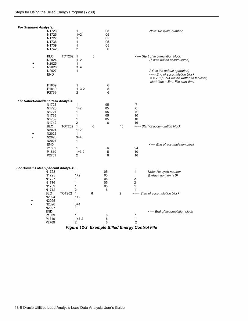
Steps for Using the Billed Energy Program (Y230)
Figure 12-2 Example Billed Energy Control File
For Standard Analysis:N1723 1 05 Note: No cycle-numberN1725 1+2 05N1727 1 05N1736 1 05N1739 1 05N1742 2 6
BLO TOT202 1 6 <---- Start of accumulation blockN2024 1+2 (6 cuts will be accumulated)
+ N2025 1- N2026 3+4
N2027 1 (“+” is the default operation)END <---- End of accumulation block
TOT202,1 cut will be written to tableset; start-time = Env. File start-time
P1809 1 6P1810 1+3-2 5P2769 2 6
For Ratio/Coincident Peak Analysis:N1723 1 05 7N1725 1+2 05 6N1727 1 05 5N1736 1 05 10N1739 1 05 10N1742 2 6 16BLO TOT202 1 6 16 <---- Start of accumulation blockN2024 1+2
+ N2025 1- N2026 3+4
N2027 1END <---- End of accumulation blockP1809 1 6 24P1810 1+3-2 5 10P2769 2 6 16
For Domains Mean-per-Unit Analysis:N1723 1 05 1 Note: No cycle numberN1725 1+2 05 (Default domain is 0)N1727 1 05 2N1736 1 05 2N1739 1 05 1N1742 2 6 1BLO TOT202 1 6 2 <---- Start of accumulation blockN2024 1+2
+ N2025 1- N2026 3+4
N2027 1END <---- End of accumulation blockP1809 1 6 1P1810 1+3-2 5 1P2769 2 6 2
13-6 Oracle Utilities Load Analysis Load Data Analysis User’s Guide
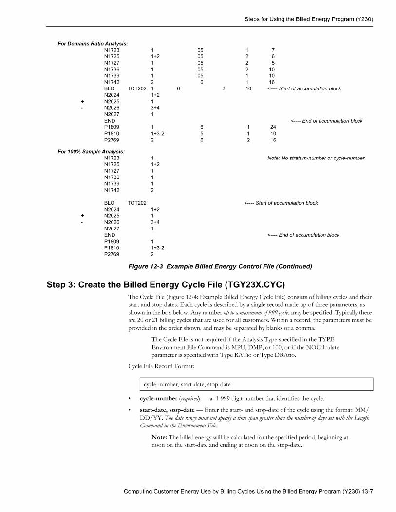
Steps for Using the Billed Energy Program (Y230)
Figure 12-3 Example Billed Energy Control File (Continued)
Step 3: Create the Billed Energy Cycle File (TGY23X.CYC)The Cycle File (Figure 12-4: Example Billed Energy Cycle File) consists of billing cycles and their start and stop dates. Each cycle is described by a single record made up of three parameters, as shown in the box below. Any number up to a maximum of 999 cycles may be specified. Typically there are 20 or 21 billing cycles that are used for all customers. Within a record, the parameters must be provided in the order shown, and may be separated by blanks or a comma.
The Cycle File is not required if the Analysis Type specified in the TYPE Environment File Command is MPU, DMP, or 100, or if the NOCalculate parameter is specified with Type RATio or Type DRAtio.
Cycle File Record Format:
• cycle-number (required) — a 1-999 digit number that identifies the cycle.
• start-date, stop-date — Enter the start- and stop-date of the cycle using the format: MM/DD/YY. The date range must not specify a time span greater than the number of days set with the Length Command in the Environment File.
Note: The billed energy will be calculated for the specified period, beginning at noon on the start-date and ending at noon on the stop-date.
For Domains Ratio Analysis:N1723 1 05 1 7N1725 1+2 05 2 6N1727 1 05 2 5N1736 1 05 2 10N1739 1 05 1 10N1742 2 6 1 16BLO TOT202 1 6 2 16 <---- Start of accumulation blockN2024 1+2
+ N2025 1- N2026 3+4
N2027 1END <---- End of accumulation blockP1809 1 6 1 24P1810 1+3-2 5 1 10P2769 2 6 2 16
For 100% Sample Analysis:N1723 1 Note: No stratum-number or cycle-numberN1725 1+2N1727 1N1736 1N1739 1N1742 2
BLO TOT202 <---- Start of accumulation blockN2024 1+2
+ N2025 1- N2026 3+4
N2027 1END <---- End of accumulation blockP1809 1P1810 1+3-2P2769 2
cycle-number, start-date, stop-date
Computing Customer Energy Use by Billing Cycles Using the Billed Energy Program (Y230) 13-7
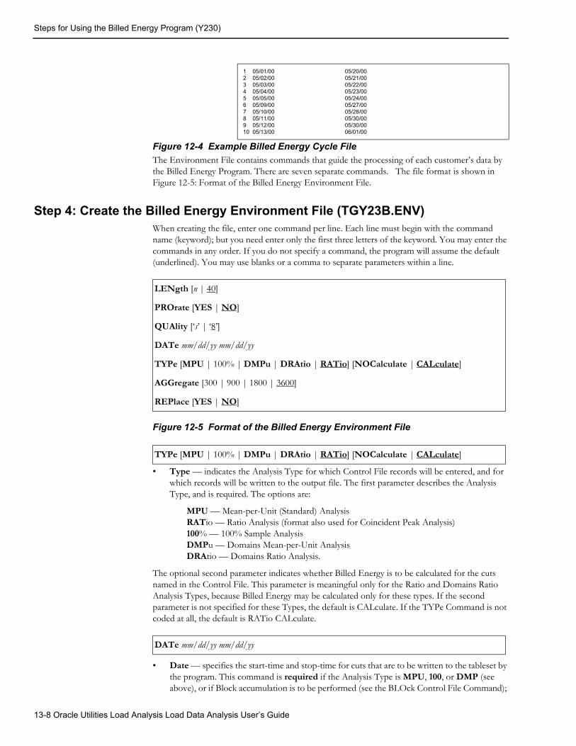
Steps for Using the Billed Energy Program (Y230)
Figure 12-4 Example Billed Energy Cycle FileThe Environment File contains commands that guide the processing of each customer’s data by the Billed Energy Program. There are seven separate commands. The file format is shown in Figure 12-5: Format of the Billed Energy Environment File.
Step 4: Create the Billed Energy Environment File (TGY23B.ENV)When creating the file, enter one command per line. Each line must begin with the command name (keyword); but you need enter only the first three letters of the keyword. You may enter the commands in any order. If you do not specify a command, the program will assume the default (underlined). You may use blanks or a comma to separate parameters within a line.
Figure 12-5 Format of the Billed Energy Environment File
• Type — indicates the Analysis Type for which Control File records will be entered, and for which records will be written to the output file. The first parameter describes the Analysis Type, and is required. The options are:
MPU — Mean-per-Unit (Standard) AnalysisRATio — Ratio Analysis (format also used for Coincident Peak Analysis)100% — 100% Sample AnalysisDMPu — Domains Mean-per-Unit AnalysisDRAtio — Domains Ratio Analysis.
The optional second parameter indicates whether Billed Energy is to be calculated for the cuts named in the Control File. This parameter is meaningful only for the Ratio and Domains Ratio Analysis Types, because Billed Energy may be calculated only for these types. If the second parameter is not specified for these Types, the default is CALculate. If the TYPe Command is not coded at all, the default is RATio CALculate.
• Date — specifies the start-time and stop-time for cuts that are to be written to the tableset by the program. This command is required if the Analysis Type is MPU, 100, or DMP (see above), or if Block accumulation is to be performed (see the BLOck Control File Command);
1 05/01/00 05/20/002 05/02/00 05/21/003 05/03/00 05/22/004 05/04/00 05/23/005 05/05/00 05/24/006 05/09/00 05/27/007 05/10/00 05/28/008 05/11/00 05/30/009 05/12/00 05/30/0010 05/13/00 06/01/00
LENgth [n | 40]
PROrate [YES | NO]
QUAlity [‘s’ | ‘8’]
DATe mm/dd/yy mm/dd/yy
TYPe [MPU | 100% | DMPu | DRAtio | RATio] [NOCalculate | CALculate]
AGGregate [300 | 900 | 1800 | 3600]
REPlace [YES | NO]
TYPe [MPU | 100% | DMPu | DRAtio | RATio] [NOCalculate | CALculate]
DATe mm/dd/yy mm/dd/yy
13-8 Oracle Utilities Load Analysis Load Data Analysis User’s Guide
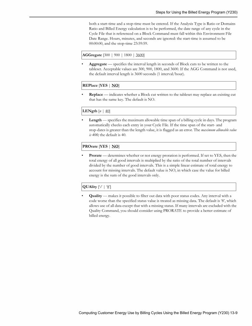
Steps for Using the Billed Energy Program (Y230)
both a start-time and a stop-time must be entered. If the Analysis Type is Ratio or Domains Ratio and Billed Energy calculation is to be performed, the date range of any cycle in the Cycle File that is referenced on a Block Command must fall within this Environment File Date Range. Hours, minutes, and seconds are ignored: the start-time is assumed to be 00:00:00, and the stop-time 23:59:59.
• Aggregate — specifies the interval length in seconds of Block cuts to be written to the tableset. Acceptable values are 300, 900, 1800, and 3600. If the AGG Command is not used, the default interval length is 3600 seconds (1 interval/hour).
• Replace — indicates whether a Block cut written to the tableset may replace an existing cut that has the same key. The default is NO.
• Length — specifies the maximum allowable time span of a billing cycle in days. The program automatically checks each entry in your Cycle File. If the time span of the start- and stop-dates is greater than the length value, it is flagged as an error. The maximum allowable value is 400; the default is 40.
• Prorate — determines whether or not energy proration is performed. If set to YES, then the total energy of all good intervals is multiplied by the ratio of the total number of intervals divided by the number of good intervals. This is a simple linear estimate of total energy to account for missing intervals. The default value is NO, in which case the value for billed energy is the sum of the good intervals only.
• Quality — makes it possible to filter out data with poor status codes. Any interval with a code worse than the specified status value is treated as missing data. The default is ‘8’, which allows use of all data except that with a missing status. If many intervals are excluded with the Quality Command, you should consider using PRORATE to provide a better estimate of billed energy.
AGGregate [300 | 900 | 1800 | 3600]
REPlace [YES | NO]
LENgth [n | 40]
PROrate [YES | NO]
QUAlity [‘s’ | ‘8’]
Computing Customer Energy Use by Billing Cycles Using the Billed Energy Program (Y230) 13-9

Steps for Using the Billed Energy Program (Y230)
Step 5: Run the Billed Energy Program (Y230)Once you have created the necessary input files, you are ready to run the program. Use Y230.
Billed Energy Program ProcessingThe Environment File is read first. Each command is processed, and defaults are used for any commands not specified. An Environment Report is printed with each command, providing its values and any error messages. If an error occurs, the program stops; otherwise, it reads the Cycle File, if required (for example, if the Analysis Type is Ratio or Domains Ratio and NOCalculate has been specified). Cycles are processed and checked. The Cycle Report mirrors the start and stop dates of each cycle, with any error messages included. If an error is encountered, the program stops.
The primary processing is driven by the Control File. Each record is read and checked. When a Block record is read, if Billed Energy is to be calculated, the date range of the cycle specified is checked to make sure it is within the Environment File date range, and an accumulation array allocated. When an Individual Customer record is read within an accumulation block (between a Block and an End record), the tableset is read for that customer-id and channel over the Environment File date range, and its energy is either added to or subtracted from the Block accumulation array. For a valid Individual Customer record that is not within an accumulation block, if the CALculate option is in effect, the appropriate cycle dates are accessed. Intervals from noon on the cycle start date to noon on the cycle stop date are read from the tableset. All intervals with status codes equal to or better than the Quality parameter are totaled for the period. If proration is requested, this total is multiplied by the number of intervals in the period divided by the number of good intervals totaled. Note that if the number of good intervals is small in comparison to the total intervals, the prorated energy estimate may not accurately reflect customer usage.
When an End record is read, a cut is created for the customer-id and channel indicated on the preceding Block Command, and the start time from the Date Command, containing the energy accumulated from individual cuts in the accumulation block. This cut is written to the tableset, and is then processed by the Billed Energy Program in the same manner as an (unblocked) Individual Customer cut.
Corresponding to each Control File input record are one or more output lines in the Execution Log. For each Individual Customer record, there is a line showing the input values, any error messages, and, for a record that is not within an accumulation block, the computed billed energy if the CALculate option was in effect. No calculated billed energy is shown for a record within an accumulation block. Errors may occur if the input parameters are incorrect, the cycle number does not correspond to a Cycle File entry, or if the data cannot be found in the tableset. A Block record triggers the printing of a block separation line, as well as the input information from the Block Command and the new block cut’s start-time (as determined by the Date Command). An End Command produces another block separation line, followed by a line indicating the processing of the block accumulation cut written to the tableset, if block processing was successful.
If no error occurs in the processing of either an unblocked Individual Customer record or an entire accumulation block, then an output record is created for analysis. The output record’s format depends on the Analysis Type and Calculate/Nocalculate status. An output record is created for an Individual Customer record that is not part of an accumulation block, a single block output record is created for an accumulation block, using the customer-id and channel provided on the Block Command. No output record is created for a customer or a block for which a processing error is reported in the Execution Log.
13-10 Oracle Utilities Load Analysis Load Data Analysis User’s Guide

Chapter 14Key Generators — Shortcuts for Creating Input
Files and Reports
This chapter explains how to work with the Key Generator programs. These programs enable you to create lists of records that match user-defined criteria. They are particularly useful for quickly generating Control files for other programs — such as Load Data Extraction, Standard Load Analysis, Ratio Analysis, Load Data Editor, and the Reporter programs.
Because these programs are very powerful, they are somewhat complex. It is recommended that you read this chapter carefully — with special attention to the section on the Control Language — before actually using them.
Topics covered in this chapter are:
• What Is the Purpose of Key Generators?
• Introducing the Control Language
• Control Language — Logic and Structure
• Sample Control Files for Key Generators
• Using the Key Generator Programs
Key Generators — Shortcuts for Creating Input Files and Reports 14-1

What Is the Purpose of Key Generators?
What Is the Purpose of Key Generators?Suppose that you have been asked to analyze the load pattern for your utility’s residential customers with all electric heating. One of your first tasks would be to get a list of the appropriate customers in the sample and to input their IDs in a Control File for the Analysis program. It could be a long and time-consuming process to look up each customer’s end-use and manually type in each key.
Fortunately, Oracle Utilities Load Analysis can perform tasks like these for you automatically. The system includes a set of programs that enable you to quickly identify and list customers and tableset records that match user-defined criteria. The programs are very flexible and the specific criteria are up to you. You can request that the lists be output as reports, or as files that you can, in turn, use as Control files for other programs.
The programs are called the “Key Generator programs.” The Key Generator programs allow you to request a list of cut keys, statistics identifiers, or edit blocks on the basis of any field or fields that exist in the standard Oracle Utilities Load Analysis Load Data Records or Statistics Records. For example, you can ask for all customers that have a particular identifier code, or all cuts that have a forced merge field, or all cuts that have a particular start-date, or all statistics from a particular class load study.
You may also create your own output CSV file containing specific and customized information about any cut in the tablesets.
The following pages provide an introduction to the Key Generator program. We will first take a close look at the Control Language that enables you to construct your data requests in the programs. Then we will go through the steps for actually using the program.
14-2 Oracle Utilities Load Analysis Load Data Analysis User’s Guide
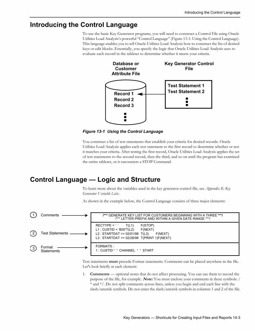
Introducing the Control Language
Introducing the Control LanguageTo use the basic Key Generator programs, you will need to construct a Control File using Oracle Utilities Load Analysis’s powerful “Control Language” (Figure 13-1: Using the Control Language). This language enables you to tell Oracle Utilities Load Analysis how to construct the list of desired keys or edit blocks. Essentially, you specify the logic that Oracle Utilities Load Analysis uses to evaluate each record in the tableset to determine whether it meets your criteria.
Figure 13-1 Using the Control Language
You construct a list of test statements that establish your criteria for desired records. Oracle Utilities Load Analysis applies each test statement to the first record to determine whether or not it matches your criteria. After testing the first record, Oracle Utilities Load Analysis applies the set of test statements to the second record, then the third, and so on until the program has examined the entire tableset, or it encounters a STOP Command.
Control Language — Logic and StructureTo learn more about the variables used in the key generator control file, see Appendix K: Key Generator Variable Lists.
As shown in the example below, the Control Language consists of three major elements:
Test statements must precede Format statements. Comments can be placed anywhere in the file. Let’s look briefly at each element:
1. Comments — optional notes that do not affect processing. You can use them to record the purpose of the file, for example. Note: You must enclose your comments in these symbols: /* and */. Do not split comments across lines, unless you begin and end each line with the slash/asterisk symbols. Do not enter the slash/asterisk symbols in columns 1 and 2 of the file.
Key Generator Control File
Record 1Record 2Record 3
Test Statement 1Test Statement 2
Database orCustomer
Attribute File
Comments
RECTYPE = ‘ ‘ T(L1) F(STOP)L1 : CUSTID = ‘B00’T(L2) F(NEXT)L2 : STARTDAT >= 02/01/98 T(L3) F(NEXT)L3 : STARTDAT <= 02/28/98 T(PRINT 1)F(NEXT)
FORMATS :1 : CUSTID ‘ ’ CHANNEL ‘ ’ START
/*** GENERATE KEY LIST FOR CUSTOMERS BEGINNING WITH A THREE ***//*** LETTER PREFIX AND WITHIN A GIVEN DATE RANGE ***/
Test Statements
FormatStatements
1
2
3
Key Generators — Shortcuts for Creating Input Files and Reports 14-3
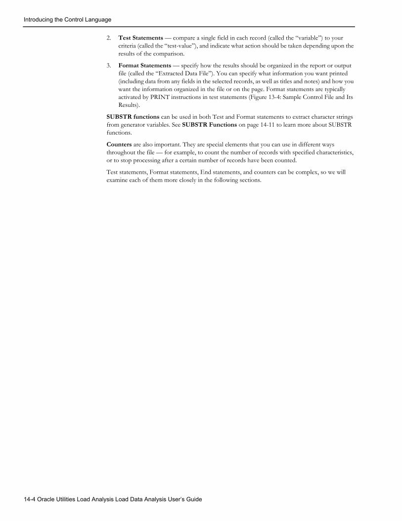
Introducing the Control Language
2. Test Statements — compare a single field in each record (called the “variable”) to your criteria (called the “test-value”), and indicate what action should be taken depending upon the results of the comparison.
3. Format Statements — specify how the results should be organized in the report or output file (called the “Extracted Data File”). You can specify what information you want printed (including data from any fields in the selected records, as well as titles and notes) and how you want the information organized in the file or on the page. Format statements are typically activated by PRINT instructions in test statements (Figure 13-4: Sample Control File and Its Results).
SUBSTR functions can be used in both Test and Format statements to extract character strings from generator variables. See SUBSTR Functions on page 14-11 to learn more about SUBSTR functions.
Counters are also important. They are special elements that you can use in different ways throughout the file — for example, to count the number of records with specified characteristics, or to stop processing after a certain number of records have been counted.
Test statements, Format statements, End statements, and counters can be complex, so we will examine each of them more closely in the following sections.
14-4 Oracle Utilities Load Analysis Load Data Analysis User’s Guide
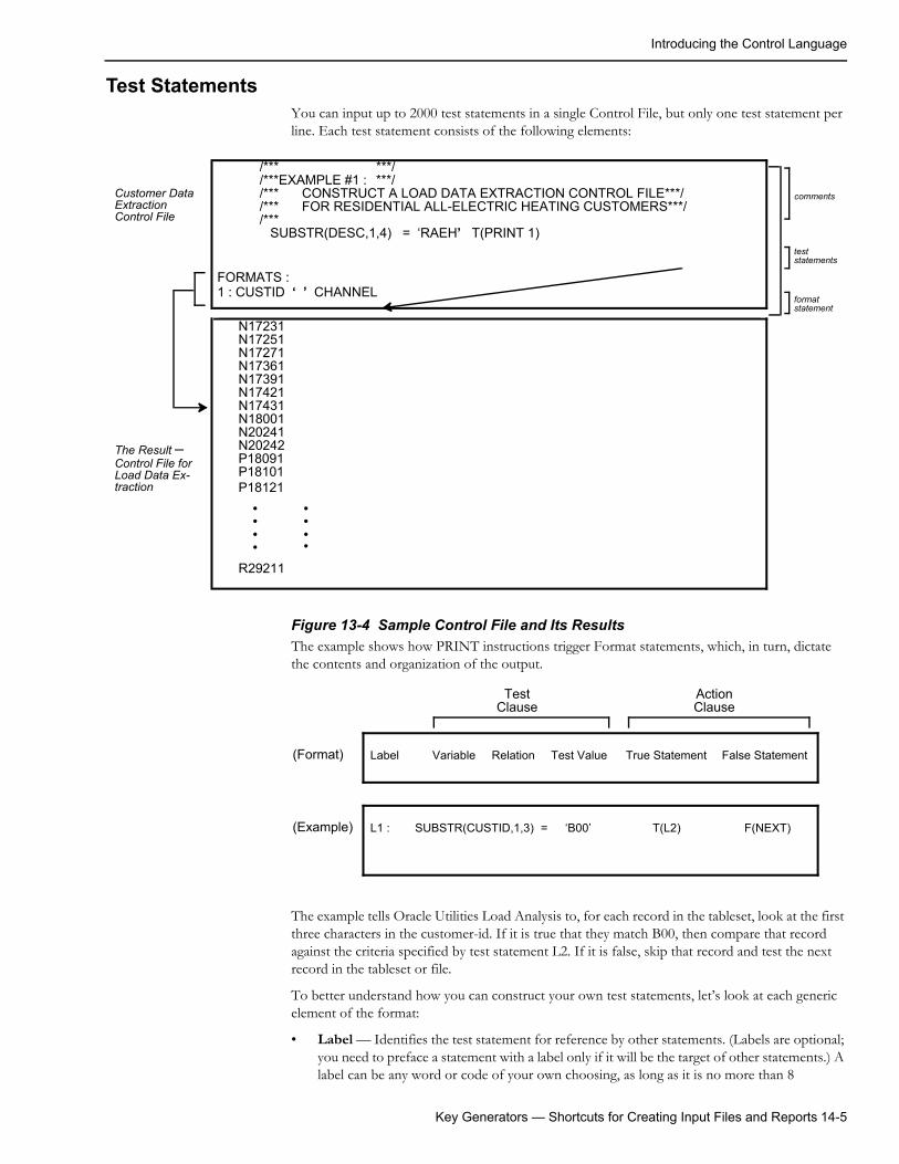
Introducing the Control Language
Test StatementsYou can input up to 2000 test statements in a single Control File, but only one test statement per line. Each test statement consists of the following elements:
Figure 13-4 Sample Control File and Its ResultsThe example shows how PRINT instructions trigger Format statements, which, in turn, dictate the contents and organization of the output.
The example tells Oracle Utilities Load Analysis to, for each record in the tableset, look at the first three characters in the customer-id. If it is true that they match B00, then compare that record against the criteria specified by test statement L2. If it is false, skip that record and test the next record in the tableset or file.
To better understand how you can construct your own test statements, let’s look at each generic element of the format:
• Label — Identifies the test statement for reference by other statements. (Labels are optional; you need to preface a statement with a label only if it will be the target of other statements.) A label can be any word or code of your own choosing, as long as it is no more than 8
/*** ***//***EXAMPLE #1 : ***//*** CONSTRUCT A LOAD DATA EXTRACTION CONTROL FILE***//*** FOR RESIDENTIAL ALL-ELECTRIC HEATING CUSTOMERS***//***
SUBSTR(DESC,1,4) = ‘RAEH’ T(PRINT 1)
FORMATS :1 : CUSTID ‘ ’ CHANNEL
N17231N17251N17271N17361N17391N17421N17431N18001N20241N20242P18091P18101P18121
R29211
••••••••
The Result –Control File for Load Data Ex-traction
teststatements
formatstatement
commentsCustomer DataExtractionControl File
Label Variable Relation Test Value True Statement False Statement(Format)
Test Clause
Action Clause
L1 :(Example) ‘B00’SUBSTR(CUSTID,1,3) = T(L2) F(NEXT)
Key Generators — Shortcuts for Creating Input Files and Reports 14-5
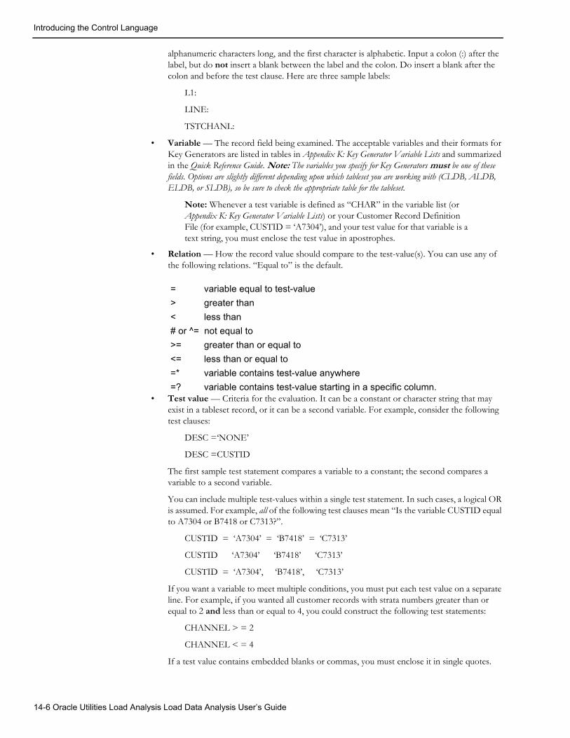
Introducing the Control Language
alphanumeric characters long, and the first character is alphabetic. Input a colon (:) after the label, but do not insert a blank between the label and the colon. Do insert a blank after the colon and before the test clause. Here are three sample labels:
L1:
LINE:
TSTCHANL:
• Variable — The record field being examined. The acceptable variables and their formats for Key Generators are listed in tables in Appendix K: Key Generator Variable Lists and summarized in the Quick Reference Guide. Note: The variables you specify for Key Generators must be one of these fields. Options are slightly different depending upon which tableset you are working with (CLDB, ALDB, ELDB, or SLDB), so be sure to check the appropriate table for the tableset.
Note: Whenever a test variable is defined as “CHAR” in the variable list (or Appendix K: Key Generator Variable Lists) or your Customer Record Definition File (for example, CUSTID = ‘A7304’), and your test value for that variable is a text string, you must enclose the test value in apostrophes.
• Relation — How the record value should compare to the test-value(s). You can use any of the following relations. “Equal to” is the default.
• Test value — Criteria for the evaluation. It can be a constant or character string that may exist in a tableset record, or it can be a second variable. For example, consider the following test clauses:
DESC =‘NONE’
DESC =CUSTID
The first sample test statement compares a variable to a constant; the second compares a variable to a second variable.
You can include multiple test-values within a single test statement. In such cases, a logical OR is assumed. For example, all of the following test clauses mean “Is the variable CUSTID equal to A7304 or B7418 or C7313?”.
CUSTID = ‘A7304’ = ‘B7418’ = ‘C7313’
CUSTID ‘A7304’ ‘B7418’ ‘C7313’
CUSTID = ‘A7304’, ‘B7418’, ‘C7313’
If you want a variable to meet multiple conditions, you must put each test value on a separate line. For example, if you wanted all customer records with strata numbers greater than or equal to 2 and less than or equal to 4, you could construct the following test statements:
CHANNEL > = 2
CHANNEL < = 4
If a test value contains embedded blanks or commas, you must enclose it in single quotes.
= variable equal to test-value> greater than< less than# or ^= not equal to>= greater than or equal to<= less than or equal to=* variable contains test-value anywhere=? variable contains test-value starting in a specific column.
14-6 Oracle Utilities Load Analysis Load Data Analysis User’s Guide
Introducing the Control Language
Before we go on, let’s look at a few more sample test clauses and their meanings (test clauses are a subset of the test statement and consist of a variable, relation, and one or more test values).
• Wild cards — A “wild card” feature allows you to find particular characters within a variable. The “=*” operator enables you to find the test value anywhere in the variable. For example, the following test clause means “Does the variable CUSTID Contain AGG?”:
CUSTID =* AGG
Another option, the “=?” operator, allows you to find the test value starting in a specific column. To use this positional wildcard operator, the test value is specified with placeholders (“?”) preceding the starting column. For example, the following test clause means “Does the variable CUSTID contain AGG starting in column 4?”:
CUSTID =? ???AGG
The wildcard feature can only be used on variables that are defined as character. See the variable lists in Appendix K: Key Generator Variable Lists.
• True and False clauses — True clauses specify the action the program will take if a record matches the criteria. False clauses specify the action the program will take if a record does not match the criteria. Possible actions are:
Output one or more fields from the record (PRINT)
Count occurrence (COUNT)
Continue with the next test (continue)
Restart the test with the next record (NEXT)
Branch forward to another test statement (label)
Terminate the program (STOP)
A combination of the above.
Here is a summary of the format you will use for constructing the clauses.
Note: True clauses must be preceded by the prefix “T” and false clauses by “F”. Parentheses must enclose the clauses. Do not insert a blank between the prefix and the left parenthesis.
PRINT n tells Oracle Utilities Load Analysis to write data from the record to a file or report, using the format you specify in Format Statement “n”. (Input the word “PRINT” followed by a blank and the Format Statement number “n”.)
COUNTm tells Oracle Utilities Load Analysis to count the number of occurrences of the condition you specified in the test statement. You can have multiple counters in a Control File; use an integer “m” to distinguish between them. (Input the word “COUNT” followed by an integer
True Clause:
T ( [PRINT n] [,COUNT m] [,label | ,STOP | ,NEXT | , continue] )
False Clause:
F ( [PRINT n] [,COUNT m] [,label | ,STOP | ,NEXT ] )
CHANNEL # 1 Is the variable CHANNEL not equal to 1?
DESC = ‘RAEH’, ‘RHWH’Is the variable DESC equal to theconstant RAEH or RHWH?
DESC = CUSTID, ‘TEMP05’Is the variable DESC equal to thevariable CUSTID or the constantTEMP05?
Key Generators — Shortcuts for Creating Input Files and Reports 14-7
Introducing the Control Language
“m”.) Note: For a more complete description of what you can do with COUNTm, see Counter Variables on page 14-12. “m” can be a value between 1 and 999.
NEXT tells Oracle Utilities Load Analysis to stop evaluating the current record and compare the next record with the first test statement. This action is the default for all false clauses, and for the last true clause in the file. (For true clauses, input the word “NEXT”; for false clauses, no input is required.)
label tells Oracle Utilities Load Analysis to compare the current record with the test statement prefixed by “label”. (Input your designation for the label. Note: The labelled statement must occur below the clause; in other words, only “forward” branches are allowed.)
STOP tells Oracle Utilities Load Analysis to stop the program whenever the condition specified has been met. STOP is useful when searching for one particular record; there is no need to scan the remaining records after finding the desired record. (Input the word “STOP”.)
continue tells Oracle Utilities Load Analysis to compare the current record with the next test statement. This action is possible only for true clauses, and is the default for all true clauses except the last one in the file. (Because it is the default, no entry is required. Do not input the word “continue”.) To continue when a false clause is executed, you must put in the label of the next statement.
You can include the “COUNTm” and “PRINT n” clauses with any one of the other four clauses in the same statement. However, the “continue”, “STOP”, “NEXT”, and “LABEL” clauses are mutually exclusive.
Logically, each test statement must have one true clause and one false clause. However, in many cases you will not need to actually input both, because you can often rely on the defaults.
Oracle Utilities Load Analysis will compare each record against the entire set of test statements until it reaches a STOP Statement or the end of the tableset. It will then output the results according to the instructions you provide in the Format statements.
Some Tips on Constructing Test StatementsBefore going on to the Format statements, let’s look at a few sample test statements. These samples show that there can be many ways of setting up the test statements to accomplish the same task, but you must be careful to structure the statements to get the result you really want. In addition, some approaches are more direct and therefore easier to understand. As a general rule, it is best to construct the file with the fewest possible statements, and to set the clauses to match desired conditions.
In the following examples, our task is to direct the program to print data from all records that have strata numbers 2 through 10. The first two statements will yield the proper results; the third will not.
14-8 Oracle Utilities Load Analysis Load Data Analysis User’s Guide
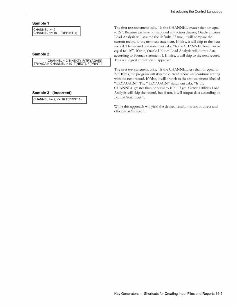
Introducing the Control Language
CHANNEL >= 2CHANNEL <= 10 T(PRINT 1)
The first test statement asks, “Is the CHANNEL greater than or equalto 2?”. Because we have not supplied any action clauses, Oracle Utilities Load Analysis will assume the defaults. If true, it will compare the current record to the next test statement. If false, it will skip to the next record. The second test statement asks, “Is the CHANNEL less than or equal to 10?”. If true, Oracle Utilities Load Analysis will output data according to Format Statement 1. If false, it will skip to the next record. This is a logical and efficient approach.
The first test statement asks, “Is the CHANNEL less than or equal to 2?”. If yes, the program will skip the current record and continue testing with the next record. If false, it will branch to the test statement labelled “TRYAGAIN”. The “TRYAGAIN” statement asks, “Is the CHANNEL greater than or equal to 10?”. If yes, Oracle Utilities Load Analysis will skip the record, but if not, it will output data according to Format Statement 1.
While this approach will yield the desired result, it is not as direct and efficient as Sample 1.
CHANNEL < 2 T(NEXT), F(TRYAGAIN)TRYAGAIN:CHANNEL > 10 T(NEXT), F(PRINT 1)
CHANNEL >= 2, <= 10 T(PRINT 1)
Sample 1
Sample 2
Sample 3 (incorrect)
Key Generators — Shortcuts for Creating Input Files and Reports 14-9
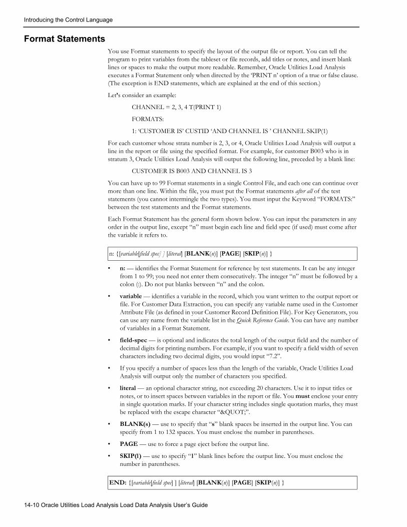
Introducing the Control Language
Format StatementsYou use Format statements to specify the layout of the output file or report. You can tell the program to print variables from the tableset or file records, add titles or notes, and insert blank lines or spaces to make the output more readable. Remember, Oracle Utilities Load Analysis executes a Format Statement only when directed by the ‘PRINT n’ option of a true or false clause. (The exception is END statements, which are explained at the end of this section.)
Let’s consider an example:
CHANNEL = 2, 3, 4 T(PRINT 1)
FORMATS:
1: ‘CUSTOMER IS’ CUSTID ‘AND CHANNEL IS ’ CHANNEL SKIP(1)
For each customer whose strata number is 2, 3, or 4, Oracle Utilities Load Analysis will output a line in the report or file using the specified format. For example, for customer B003 who is in stratum 3, Oracle Utilities Load Analysis will output the following line, preceded by a blank line:
CUSTOMER IS B003 AND CHANNEL IS 3
You can have up to 99 Format statements in a single Control File, and each one can continue over more than one line. Within the file, you must put the Format statements after all of the test statements (you cannot intermingle the two types). You must input the Keyword “FORMATS:” between the test statements and the Format statements.
Each Format Statement has the general form shown below. You can input the parameters in any order in the output line, except “n” must begin each line and field spec (if used) must come after the variable it refers to.
• n: — identifies the Format Statement for reference by test statements. It can be any integer from 1 to 99; you need not enter them consecutively. The integer “n” must be followed by a colon (:). Do not put blanks between “n” and the colon.
• variable — identifies a variable in the record, which you want written to the output report or file. For Customer Data Extraction, you can specify any variable name used in the Customer Attribute File (as defined in your Customer Record Definition File). For Key Generators, you can use any name from the variable list in the Quick Reference Guide. You can have any number of variables in a Format Statement.
• field-spec — is optional and indicates the total length of the output field and the number of decimal digits for printing numbers. For example, if you want to specify a field width of seven characters including two decimal digits, you would input “7.2”.
• If you specify a number of spaces less than the length of the variable, Oracle Utilities Load Analysis will output only the number of characters you specified.
• literal — an optional character string, not exceeding 20 characters. Use it to input titles or notes, or to insert spaces between variables in the report or file. You must enclose your entry in single quotation marks. If your character string includes single quotation marks, they must be replaced with the escape character “"”.
• BLANK(s) — use to specify that “s” blank spaces be inserted in the output line. You can specify from 1 to 132 spaces. You must enclose the number in parentheses.
• PAGE — use to force a page eject before the output line.
• SKIP(l) — use to specify “l” blank lines before the output line. You must enclose the number in parentheses.
n: {[variable[field spec] ] [literal] [BLANK(n)] [PAGE] [SKIP(n)] }
END: {[variable[field spec] ] [literal] [BLANK(n)] [PAGE] [SKIP(n)] }
14-10 Oracle Utilities Load Analysis Load Data Analysis User’s Guide
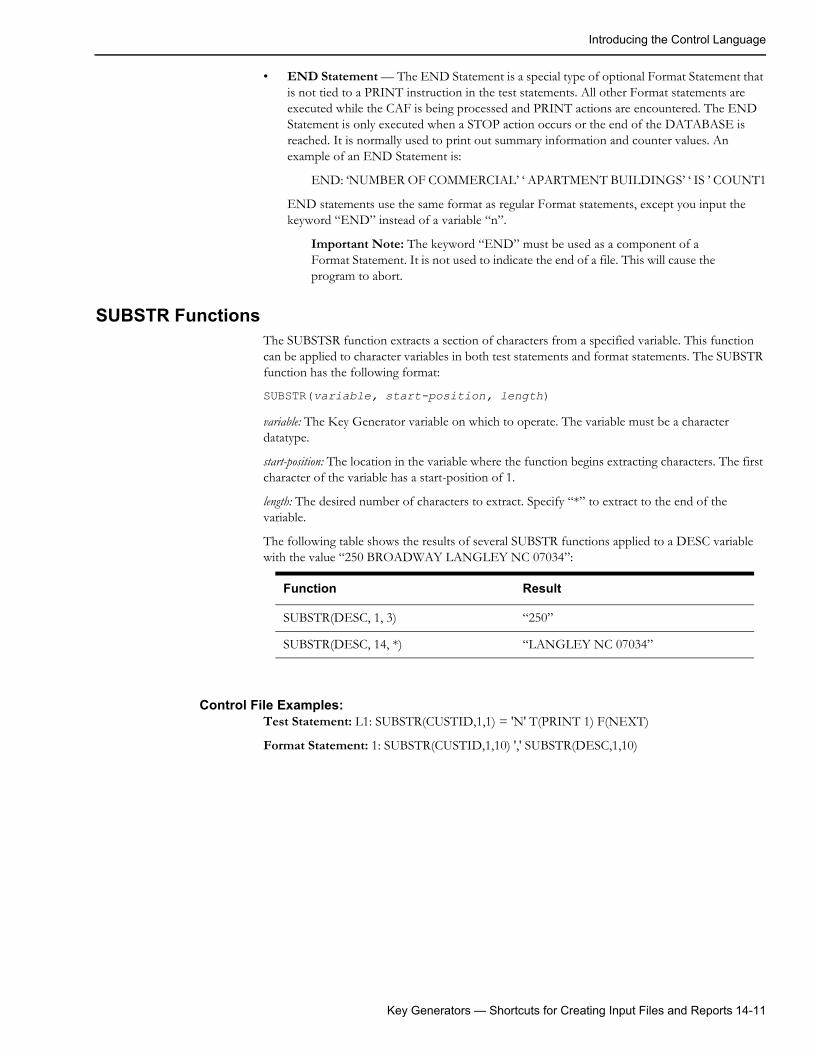
Introducing the Control Language
• END Statement — The END Statement is a special type of optional Format Statement that is not tied to a PRINT instruction in the test statements. All other Format statements are executed while the CAF is being processed and PRINT actions are encountered. The END Statement is only executed when a STOP action occurs or the end of the DATABASE is reached. It is normally used to print out summary information and counter values. An example of an END Statement is:
END: ‘NUMBER OF COMMERCIAL’ ‘ APARTMENT BUILDINGS’ ‘ IS ’ COUNT1
END statements use the same format as regular Format statements, except you input the keyword “END” instead of a variable “n”.
Important Note: The keyword “END” must be used as a component of a Format Statement. It is not used to indicate the end of a file. This will cause the program to abort.
SUBSTR FunctionsThe SUBSTSR function extracts a section of characters from a specified variable. This function can be applied to character variables in both test statements and format statements. The SUBSTR function has the following format:
SUBSTR(variable, start-position, length)
variable: The Key Generator variable on which to operate. The variable must be a character datatype.
start-position: The location in the variable where the function begins extracting characters. The first character of the variable has a start-position of 1.
length: The desired number of characters to extract. Specify “*” to extract to the end of the variable.
The following table shows the results of several SUBSTR functions applied to a DESC variable with the value “250 BROADWAY LANGLEY NC 07034”:
Control File Examples:Test Statement: L1: SUBSTR(CUSTID,1,1) = 'N' T(PRINT 1) F(NEXT)
Format Statement: 1: SUBSTR(CUSTID,1,10) ',' SUBSTR(DESC,1,10)
Function Result
SUBSTR(DESC, 1, 3) “250”
SUBSTR(DESC, 14, *) “LANGLEY NC 07034”
Key Generators — Shortcuts for Creating Input Files and Reports 14-11
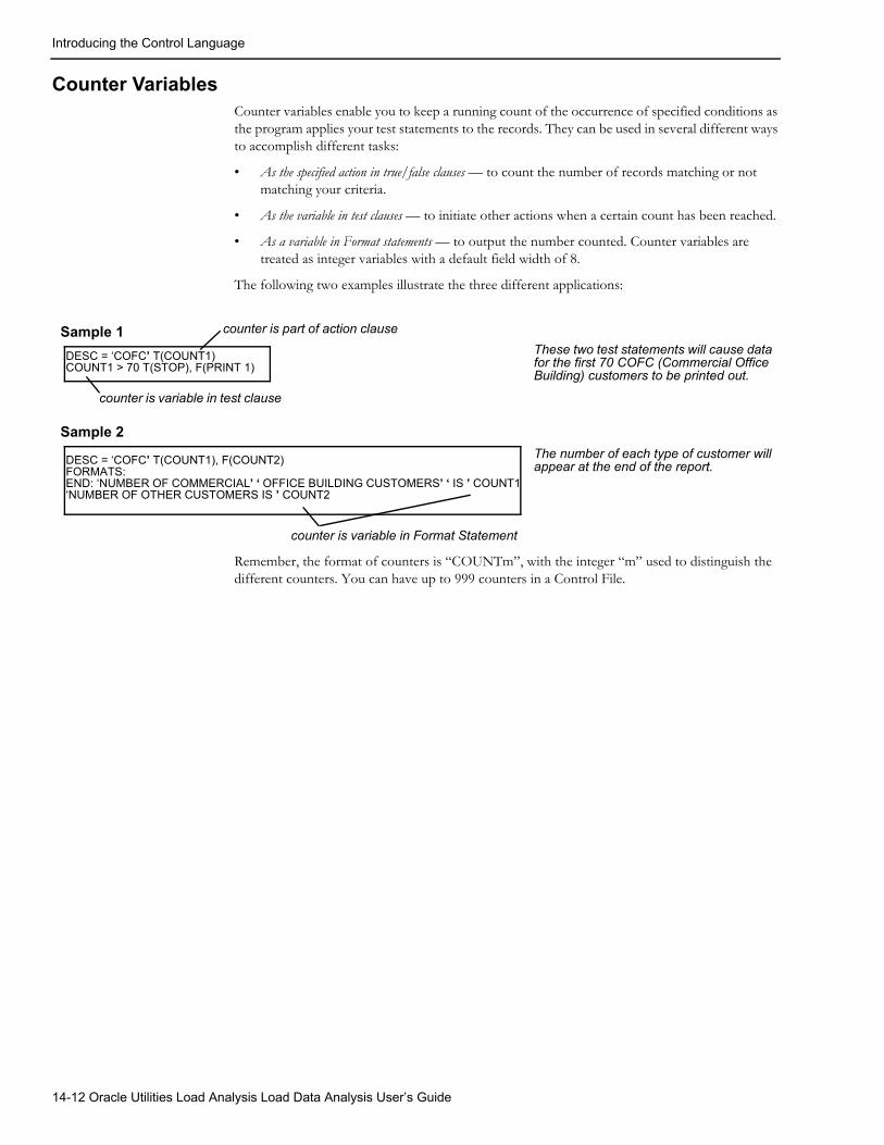
Introducing the Control Language
Counter VariablesCounter variables enable you to keep a running count of the occurrence of specified conditions as the program applies your test statements to the records. They can be used in several different ways to accomplish different tasks:
• As the specified action in true/false clauses — to count the number of records matching or not matching your criteria.
• As the variable in test clauses — to initiate other actions when a certain count has been reached.
• As a variable in Format statements — to output the number counted. Counter variables are treated as integer variables with a default field width of 8.
The following two examples illustrate the three different applications:
Remember, the format of counters is “COUNTm”, with the integer “m” used to distinguish the different counters. You can have up to 999 counters in a Control File.
DESC = ‘COFC’ T(COUNT1)COUNT1 > 70 T(STOP), F(PRINT 1)
These two test statements will cause data for the first 70 COFC (Commercial Office Building) customers to be printed out.
The number of each type of customer will appear at the end of the report.DESC = ‘COFC’ T(COUNT1), F(COUNT2)
FORMATS:END: ‘NUMBER OF COMMERCIAL’ ‘ OFFICE BUILDING CUSTOMERS’ ‘ IS ’ COUNT1‘NUMBER OF OTHER CUSTOMERS IS ’ COUNT2
Sample 1
Sample 2
counter is part of action clause
counter is variable in test clause
counter is variable in Format Statement
14-12 Oracle Utilities Load Analysis Load Data Analysis User’s Guide
Introducing the Control Language
A Checklist for Using the Control Language
Here is a summary of the rules you must follow when using the Control Language to construct your CDE or Key Generator Control files.
General
Test statements must precede Format statements. Comments can be placed anywhere in the file. To improve its appearance and readability, you may put blank lines anywhere in the file.
Comments
You must enclose your comments in these symbols: /* and */. Do not split comments across lines (unless you begin and end each line with the slash/asterisk symbols). Do not enter the slash/asterisk symbols in columns 1 or 2.
Test statements
You can have up to 2000 test statements in a single Control File, but only one test statement per line. Except where noted below, you can use blanks or commas to separate the elements of a statement to improve its appearance and readability.
Labels — can be up to 8 alphanumeric characters long, but the first character must be alphabetic. Each label must be followed by a colon; do not put blanks between the label and the colon.
Variables — must be one of the acceptable variables from the Key Generator list in the Quick Reference Guide (for Key Generators); or a variable from your utility’s Customer Attribute File (for Customer Data Extraction).
Relation — must be one of the accepted symbols: =, >, <, #, ^=, =, >=, <=, =*, =?.
Test-values — If a test-value contains embedded blanks or commas, you must enclose it in single quotes. Also, remember that if you specify multiple test-values, Oracle Utilities Load Analysis assumes that you will accept any one of them. If the positioned wildcard operator (=?) is used, the test-value should be specified with placeholders (?) preceding the starting column.
True and false clauses — You must precede each true clause with a “T” and each false clause with an “F”, and enclose each clause in parentheses. Do not put a blank between the prefix and the left parenthesis.
Each test statement must have one true and one false clause. If you do not enter them, Oracle Utilities Load Analysis will assume the default (“continue” for true clauses and “NEXT” for false clauses and the last true clause in the file).
Format statements
You can input up to 99 Format statements in a single Control File, and a single statement can take up more than one line.
The keyword “FORMATS:” must precede the Format statements.
All Format statements, except END statements, must be referenced by a PRINT instruction in the test statements.
Literals (optional character strings for notes or titles) must be enclosed in single quote marks.
Use the BLANK option, or literals, to separate output fields so that they do not run together in the output file.
Key Generators — Shortcuts for Creating Input Files and Reports 14-13
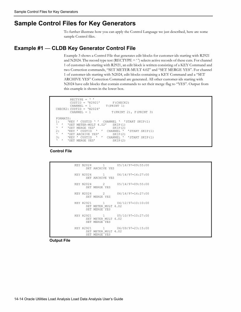
Sample Control Files for Key Generators
Sample Control Files for Key GeneratorsTo further illustrate how you can apply the Control Language we just described, here are some sample Control files.
Example #1 — CLDB Key Generator Control FileExample 3 shows a Control File that generates edit blocks for customer-ids starting with R2921 and N2024. The record type test (RECTYPE = ‘ ’) selects active records of these cuts. For channel 1 of customer-ids starting with R2921, an edit block is written consisting of a KEY Command and two Correction commands, “SET METER-MULT 4.02” and “SET MERGE YES”. For channel 1 of customer-ids starting with N2024, edit blocks containing a KEY Command and a “SET ARCHIVE YES” Correction Command are generated. All other customer-ids starting with N2024 have edit blocks that contain commands to set their merge flag to “YES”. Output from this example is shown in the lower box.
RECTYPE = ‘ ’CUSTID = ‘R2921’ F(CHECK2)CHANNEL = 1 T(PRINT 1)
CHECK2: CUSTID = ‘N2024’CHANNEL = 1 T(PRINT 2), F(PRINT 3)
FORMATS:1: ‘KEY ’ CUSTID ‘ ’ CHANNEL ‘ ’START SKIP(1)‘ ’ ‘SET METER-MULT 4.02’ SKIP(1)‘ ’ ‘SET MERGE YES’ SKIP(2)2: ‘KEY ’ CUSTID ‘ ’ CHANNEL ‘ ’START SKIP(1)‘ ’ ‘SET ARCHIVE YES’ SKIP(2)3: ‘KEY ’ CUSTID ‘ ’ CHANNEL ‘ ’START SKIP(1)‘ ’ ‘SET MERGE YES’ SKIP(2)
Control File
KEY N2024 1 05/14/97–09:55:00SET ARCHIVE YES
KEY N2024 1 06/14/97–14:27:00SET ARCHIVE YES
KEY N2024 2 05/14/97–09:55:00SET MERGE YES
KEY N2024 2 06/14/97–14:27:00SET MERGE YES
KEY R2921 1 04/12/97–10:10:00SET METER_MULT 4.02SET MERGE YES
KEY R2921 1 05/10/97–10:27:00SET METER_MULT 4.02SET MERGE YES
KEY R2921 1 06/09/97–23:15:00SET METER_MULT 4.02SET MERGE YES
Output File
14-14 Oracle Utilities Load Analysis Load Data Analysis User’s Guide
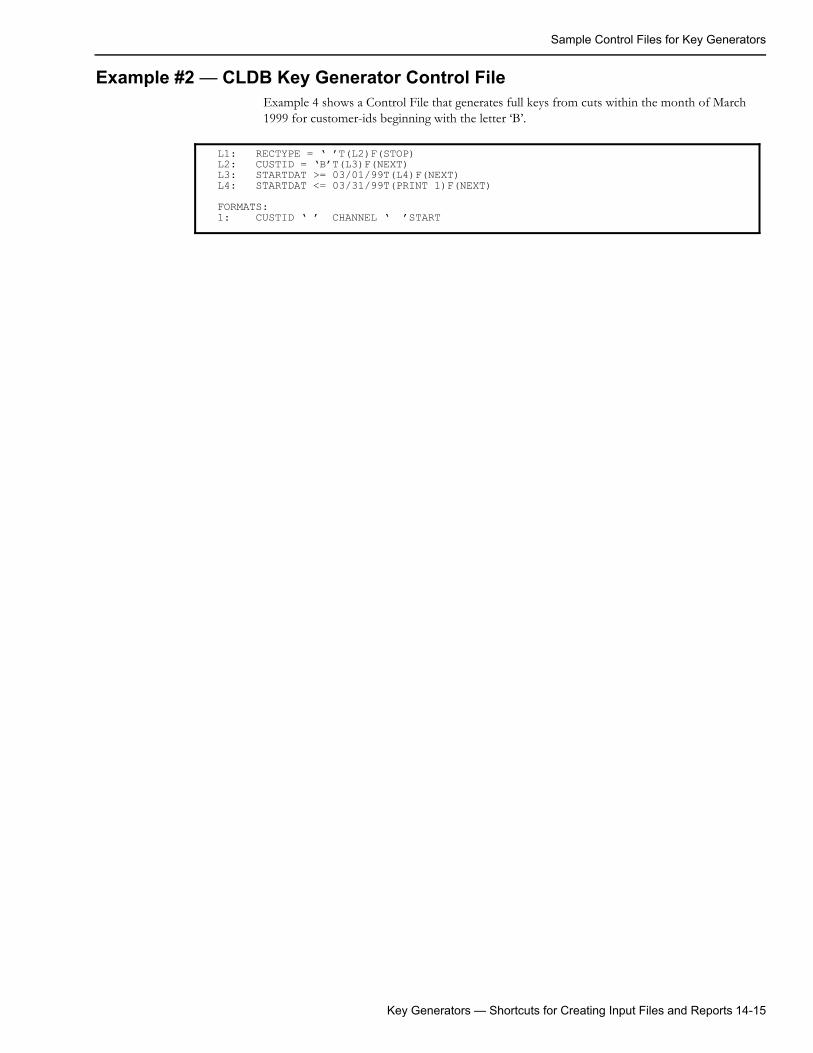
Sample Control Files for Key Generators
Example #2 — CLDB Key Generator Control FileExample 4 shows a Control File that generates full keys from cuts within the month of March 1999 for customer-ids beginning with the letter ‘B’.
L1: RECTYPE = ‘ ’T(L2)F(STOP)L2: CUSTID = ‘B’T(L3)F(NEXT)L3: STARTDAT >= 03/01/99T(L4)F(NEXT)L4: STARTDAT <= 03/31/99T(PRINT 1)F(NEXT)FORMATS:1: CUSTID ‘ ’ CHANNEL ‘ ’START
Key Generators — Shortcuts for Creating Input Files and Reports 14-15
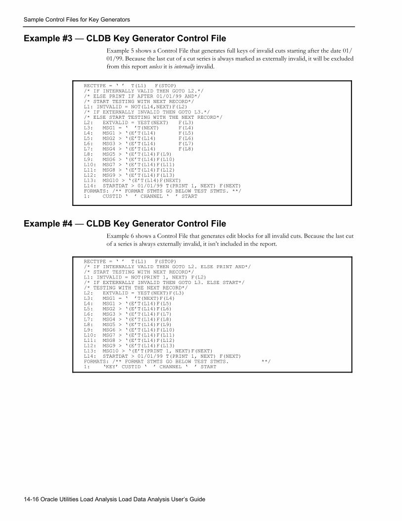
Sample Control Files for Key Generators
Example #3 — CLDB Key Generator Control FileExample 5 shows a Control File that generates full keys of invalid cuts starting after the date 01/01/99. Because the last cut of a cut series is always marked as externally invalid, it will be excluded from this report unless it is internally invalid.
Example #4 — CLDB Key Generator Control FileExample 6 shows a Control File that generates edit blocks for all invalid cuts. Because the last cut of a series is always externally invalid, it isn’t included in the report.
RECTYPE = ‘ ’ T(L1) F(STOP)/* IF INTERNALLY VALID THEN GOTO L2.*//* ELSE PRINT IF AFTER 01/01/99 AND*//* START TESTING WITH NEXT RECORD*/L1: INTVALID = NOT(L14,NEXT)F(L2)/* IF EXTERNALLY INVALID THEN GOTO L3.*//* ELSE START TESTING WITH THE NEXT RECORD*/L2: EXTVALID = YEST(NEXT) F(L3)L3: MSG1 = ‘ ’T(NEXT) F(L4)L4: MSG1 > ‘(E’T(L14) F(L5)L5: MSG2 > ‘(E’T(L14) F(L6)L6: MSG3 > ‘(E’T(L14) F(L7)L7: MSG4 > ‘(E’T(L14) F(L8)L8: MSG5 > ‘(E’T(L14)F(L9)L9: MSG6 > ‘(E’T(L14)F(L10)L10: MSG7 > ‘(E’T(L14)F(L11)L11: MSG8 > ‘(E’T(L14)F(L12)L12: MSG9 > ‘(E’T(L14)F(L13)L13: MSG10 > ‘(E’T(L14)F(NEXT)L14: STARTDAT > 01/01/99 T(PRINT 1, NEXT) F(NEXT)FORMATS: /** FORMAT STMTS GO BELOW TEST STMTS. **/1: CUSTID ‘ ’ CHANNEL ‘ ’ START
RECTYPE = ‘ ’ T(L1) F(STOP)/* IF INTERNALLY VALID THEN GOTO L2. ELSE PRINT AND*//* START TESTING WITH NEXT RECORD*/L1: INTVALID = NOT(PRINT 1, NEXT) F(L2)/* IF EXTERNALLY INVALID THEN GOTO L3. ELSE START*//* TESTING WITH THE NEXT RECORD*/L2: EXTVALID = YEST(NEXT)F(L3)L3: MSG1 = ‘ ’T(NEXT)F(L4)L4: MSG1 > ‘(E’T(L14)F(L5)L5: MSG2 > ‘(E’T(L14)F(L6)L6: MSG3 > ‘(E’T(L14)F(L7)L7: MSG4 > ‘(E’T(L14)F(L8)L8: MSG5 > ‘(E’T(L14)F(L9)L9: MSG6 > ‘(E’T(L14)F(L10)L10: MSG7 > ‘(E’T(L14)F(L11)L11: MSG8 > ‘(E’T(L14)F(L12)L12: MSG9 > ‘(E’T(L14)F(L13)L13: MSG10 > ‘(E’T(PRINT 1, NEXT)F(NEXT)L14: STARTDAT > 01/01/99 T(PRINT 1, NEXT) F(NEXT)FORMATS: /** FORMAT STMTS GO BELOW TEST STMTS. **/1: ‘KEY’ CUSTID ‘ ’ CHANNEL ‘ ’ START
14-16 Oracle Utilities Load Analysis Load Data Analysis User’s Guide
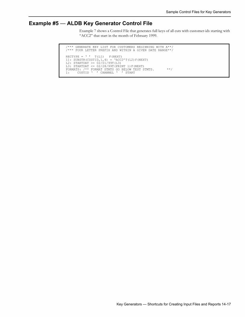
Sample Control Files for Key Generators
Example #5 — ALDB Key Generator Control FileExample 7 shows a Control File that generates full keys of all cuts with customer-ids starting with “ACC2” that start in the month of February 1999.
/*** GENERATE KEY LIST FOR CUSTOMERS BEGINNING WITH A**//*** FOUR LETTER PREFIX AND WITHIN A GIVEN DATE RANGE**/RECTYPE = ‘ ’ T(L1) F(NEXT)l1: SUBSTR(CUSTID,1,4) = ‘ACC2’T(L2)F(NEXT)L2: STARTDAT >= 02/01/99T(L3)L3: STARTDAT <= 02/28/99T(PRINT 1)F(NEXT)FORMATS: /** FORMAT STMTS GO BELOW TEST STMTS. **/1: CUSTID ‘ ’ CHANNEL ‘ ’ START
Key Generators — Shortcuts for Creating Input Files and Reports 14-17
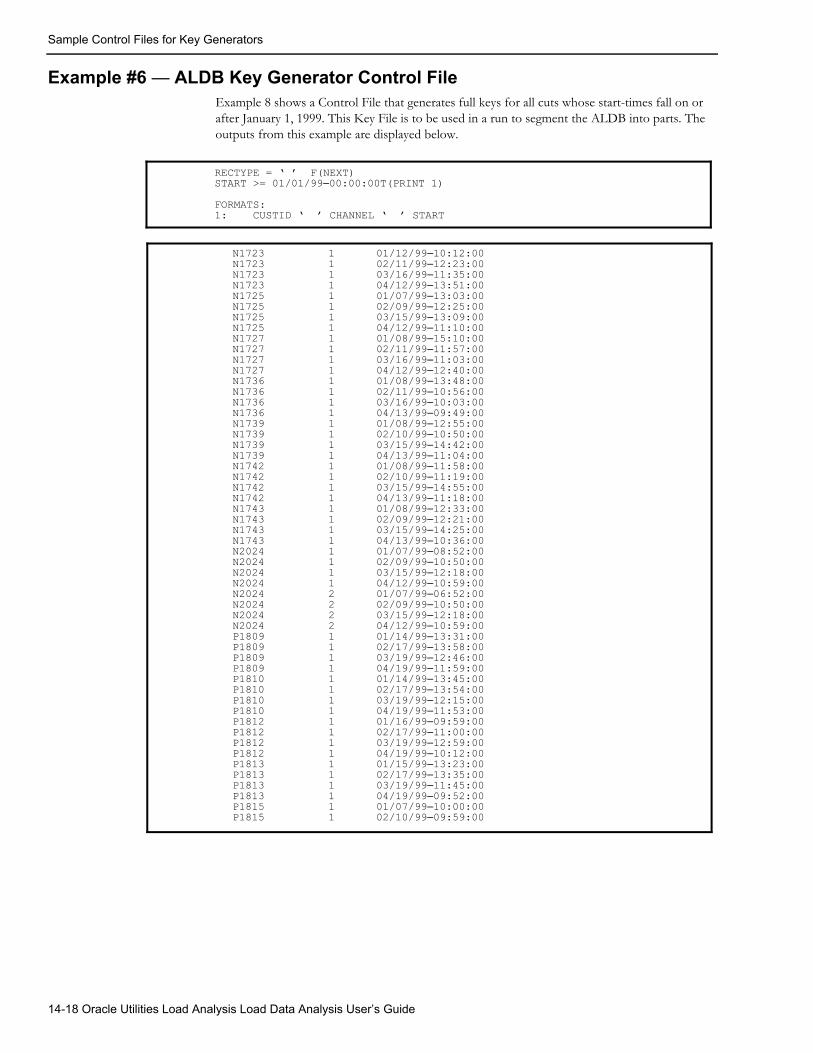
Sample Control Files for Key Generators
Example #6 — ALDB Key Generator Control FileExample 8 shows a Control File that generates full keys for all cuts whose start-times fall on or after January 1, 1999. This Key File is to be used in a run to segment the ALDB into parts. The outputs from this example are displayed below.
RECTYPE = ‘ ’ F(NEXT)START >= 01/01/99–00:00:00T(PRINT 1)FORMATS:1: CUSTID ‘ ’ CHANNEL ‘ ’ START
N1723 1 01/12/99–10:12:00N1723 1 02/11/99–12:23:00N1723 1 03/16/99–11:35:00N1723 1 04/12/99–13:51:00N1725 1 01/07/99–13:03:00N1725 1 02/09/99–12:25:00N1725 1 03/15/99–13:09:00N1725 1 04/12/99–11:10:00N1727 1 01/08/99–15:10:00N1727 1 02/11/99–11:57:00N1727 1 03/16/99–11:03:00N1727 1 04/12/99–12:40:00N1736 1 01/08/99–13:48:00N1736 1 02/11/99–10:56:00N1736 1 03/16/99–10:03:00N1736 1 04/13/99–09:49:00N1739 1 01/08/99–12:55:00N1739 1 02/10/99–10:50:00N1739 1 03/15/99–14:42:00N1739 1 04/13/99–11:04:00N1742 1 01/08/99–11:58:00N1742 1 02/10/99–11:19:00N1742 1 03/15/99–14:55:00N1742 1 04/13/99–11:18:00N1743 1 01/08/99–12:33:00N1743 1 02/09/99–12:21:00N1743 1 03/15/99–14:25:00N1743 1 04/13/99–10:36:00N2024 1 01/07/99–08:52:00N2024 1 02/09/99–10:50:00N2024 1 03/15/99–12:18:00N2024 1 04/12/99–10:59:00N2024 2 01/07/99–06:52:00N2024 2 02/09/99–10:50:00N2024 2 03/15/99–12:18:00N2024 2 04/12/99–10:59:00P1809 1 01/14/99–13:31:00P1809 1 02/17/99–13:58:00P1809 1 03/19/99–12:46:00P1809 1 04/19/99–11:59:00P1810 1 01/14/99–13:45:00P1810 1 02/17/99–13:54:00P1810 1 03/19/99–12:15:00P1810 1 04/19/99–11:53:00P1812 1 01/16/99–09:59:00P1812 1 02/17/99–11:00:00P1812 1 03/19/99–12:59:00P1812 1 04/19/99–10:12:00P1813 1 01/15/99–13:23:00P1813 1 02/17/99–13:35:00P1813 1 03/19/99–11:45:00P1813 1 04/19/99–09:52:00P1815 1 01/07/99–10:00:00P1815 1 02/10/99–09:59:00
14-18 Oracle Utilities Load Analysis Load Data Analysis User’s Guide
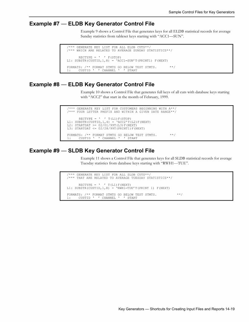
Sample Control Files for Key Generators
Example #7 — ELDB Key Generator Control FileExample 9 shows a Control File that generates keys for all ELDB statistical records for average Sunday statistics from tableset keys starting with “ACC1—SUN”.
Example #8 — ELDB Key Generator Control FileExample 10 shows a Control File that generates full keys of all cuts with database keys starting with “ACC2” that start in the month of February, 1999.
Example #9 — SLDB Key Generator Control FileExample 11 shows a Control File that generates keys for all SLDB statistical records for average Tuesday statistics from database keys starting with “RWH1—TUE”.
/*** GENERATE KEY LIST FOR ALL ELDB CUTS**//*** WHICH ARE RELATED TO AVERAGE SUNDAY STATISTICS**/
RECTYPE = ‘ ’ F(STOP)L1: SUBSTR(CUSTID,1,8) = ‘ACC1–SUN’T(PRINT1) F(NEXT)FORMATS: /** FORMAT STMTS GO BELOW TEST STMTS. **/1: CUSTID ‘ ’ CHANNEL ‘ ’ START
/*** GENERATE KEY LIST FOR CUSTOMERS BEGINNING WITH A**//*** FOUR LETTER PREFIX AND WITHIN A GIVEN DATE RANGE**/
RECTYPE = ‘ ’ T(L1)F(STOP)L1: SUBSTR(CUSTID,1,4) = ‘ACC2’T(L2)F(NEXT)L2: STARTDAT >= 02/01/99T(L3)F(NEXT)L3: STARTDAT <= 02/28/99T(PRINT1)F(NEXT)FORMATS: /** FORMAT STMTS GO BELOW TEST STMTS. **/1: CUSTID ‘ ’ CHANNEL ‘ ’ START
/*** GENERATE KEY LIST FOR ALL SLDB CUTS**//*** THAT ARE RELATED TO AVERAGE TUESDAY STATISTICS**/
RECTYPE = ‘ ’ T(L1)F(NEXT)L1: SUBSTR(CUSTID,1,8) = ‘RWH1–TUE’T(PRINT 1) F(NEXT)FORMATS: /** FORMAT STMTS GO BELOW TEST STMTS. **/1: CUSTID ‘ ’ CHANNEL ‘ ’ START
Key Generators — Shortcuts for Creating Input Files and Reports 14-19
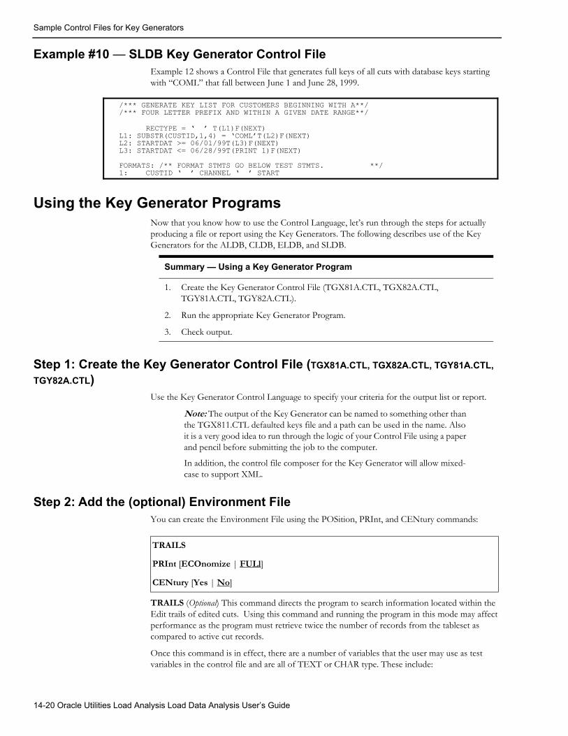
Sample Control Files for Key Generators
Example #10 — SLDB Key Generator Control FileExample 12 shows a Control File that generates full keys of all cuts with database keys starting with “COML” that fall between June 1 and June 28, 1999.
Using the Key Generator ProgramsNow that you know how to use the Control Language, let’s run through the steps for actually producing a file or report using the Key Generators. The following describes use of the Key Generators for the ALDB, CLDB, ELDB, and SLDB.
Step 1: Create the Key Generator Control File (TGX81A.CTL, TGX82A.CTL, TGY81A.CTL, TGY82A.CTL)
Use the Key Generator Control Language to specify your criteria for the output list or report.
Note: The output of the Key Generator can be named to something other than the TGX811.CTL defaulted keys file and a path can be used in the name. Also it is a very good idea to run through the logic of your Control File using a paper and pencil before submitting the job to the computer.
In addition, the control file composer for the Key Generator will allow mixed-case to support XML.
Step 2: Add the (optional) Environment FileYou can create the Environment File using the POSition, PRInt, and CENtury commands:
TRAILS (Optional) This command directs the program to search information located within the Edit trails of edited cuts. Using this command and running the program in this mode may affect performance as the program must retrieve twice the number of records from the tableset as compared to active cut records.
Once this command is in effect, there are a number of variables that the user may use as test variables in the control file and are all of TEXT or CHAR type. These include:
/*** GENERATE KEY LIST FOR CUSTOMERS BEGINNING WITH A**//*** FOUR LETTER PREFIX AND WITHIN A GIVEN DATE RANGE**/
RECTYPE = ‘ ’ T(L1)F(NEXT)L1: SUBSTR(CUSTID,1,4) = ‘COML’T(L2)F(NEXT)L2: STARTDAT >= 06/01/99T(L3)F(NEXT)L3: STARTDAT <= 06/28/99T(PRINT 1)F(NEXT)FORMATS: /** FORMAT STMTS GO BELOW TEST STMTS. **/1: CUSTID ‘ ’ CHANNEL ‘ ’ START
Summary — Using a Key Generator Program
1. Create the Key Generator Control File (TGX81A.CTL, TGX82A.CTL, TGY81A.CTL, TGY82A.CTL).
2. Run the appropriate Key Generator Program.
3. Check output.
TRAILS
PRInt [ECOnomize | FULl]
CENtury [Yes | No]
14-20 Oracle Utilities Load Analysis Load Data Analysis User’s Guide
Sample Control Files for Key Generators
• TRAILS: This test variable will define all 150 available TRAILs in a single string
• TRAILCT: This variable will define the number of edit trails associated with a cut.
• TRAIL1, TRAIL2.. TRAILn… TRAIL40: These variables will define specific edit trails up to the 40th edit trail.
The maximum number of edit trails that may be searched is the first 40.
If TRAILS is in effect, the only other cut characteristics that may be included as test or print statements (available variables) are all CUSTID variables, channel, and all parts of the start time.
The TRAIL parameter may appear in the Environment File as TRAIL or TRA.
PRInt - (Optional) This command will instruct the program to write or not write format statement data into the output report (REPORT.HTML). Print Full is the default.
FULl - Instruct the program to write into the output report the format data records satisfying the search criteria in the Control File.
ECOnomize - Instruct the program not to write into the output report the format data records satisfying the search criteria in the Control File, resulting in a smaller report.
CENtury - If this command is specified, either with the Yes option or with none, all dates written by the Key Generator will contain a 4-digit year (e.g. 1999). If the command is absent or the No option is specified, the date will contain a 2-digit year (e.g. 99).
Key Generators — Shortcuts for Creating Input Files and Reports 14-21
Sample Control Files for Key Generators
Step 3: Run the Key Generator ProgramUse the appropriate program, according to the tableset you are working with.
ALDB:(X820)CLDB:(X810)ELDB:(Y810)SLDB:(Y820)
Key Generator ProcessingThe Key Generator Program starts testing each customer record with the first test statement in the Control File. For each test statement, the value of the specified customer variable is compared to each test value in the value-list in succession. If the comparison between the customer variable and a test value matches the relation specified for that test value, the test statement is set to “TRUE” and no more test values are tried. If the value list is exhausted and no matching relationship has been found, the test statement is set to “FALSE”.
After the test statement is set to “TRUE” or “FALSE”, the action specified by the statement’s true- or false-clause is taken. Test statements continue to be executed for the customer record until an execution true- or false-clause specifies “NEXT” or all the test statements have been performed.
The next cut is then read, and the program restarts testing from the top of the Control File. The program continues in this manner until all customer records have been read or a “STOP” condition is reached. If a test-clause is not specified for a test statement, the statement is automatically set to “TRUE” and the true-clause is executed.
Step 4: Check OutputAt the end of its run, the Key Generator Program produces two outputs:
• Output Keys File — lists the cut keys that match user-defined criteria. By default the programs output this file to the Job directory, but you can specify the location of this file on the Submit Panel.
• Execution Log — lists back the Key Generator Control File and identifies any errors; includes the Extracted Data Report that lists the contents of the Output Keys File.
As with other output reports, be sure to go over each one carefully to ensure that there were no problems and the program executed successfully.
Samples of the reports follow.
14-22 Oracle Utilities Load Analysis Load Data Analysis User’s Guide
Chapter 15Performing Ad Hoc Load Calculations Using the
Transformation Program (X620, Y620)
In an earlier chapter, we saw how it is possible to use the Load Data Editor to modify cuts by specifying new values to replace old ones. The Transformation Program also enables you to modify cuts or create new ones, but the operations it performs are more complex. Specifically, you can perform arithmetic operations on the data or apply any of a set of “Transformation Functions” such as sorting, masking, or rescaling.
Topics covered are:
• What Does the Transformation Program Do?
• Using the Transformation Commands
• Steps for Using the Transformation Program
Performing Ad Hoc Load Calculations Using the Transformation Program (X620, Y620) 15-1
What Does the Transformation Program Do?
What Does the Transformation Program Do?The Transformation Program is a useful “tool kit” of commands that enable you to calculate new data from existing data in the Interval Database. For example, you can quickly apply loss factors, compute KVA, or combine multiple channels of data into a single record. The program also allows you to manipulate existing data; for instance, you can select data by TOU period or prepare cuts for graphing.
The types of transformations you can perform fall into two categories:
• Arithmetic operations — you can add, subtract, multiply, or divide cut data by other cut data or by a supplied constant. This is useful for combining channels of data or applying loss factors.
• Transformation functions — you can apply any of a series of Transformation functions to a cut. There are a variety of functions for different tasks — such as sorting, masking, and rescaling data (the complete list is shown in Figure 14-4: Table of Transformation Functions). These functions are very useful if you need to graph a demand duration curve, expand sample statistics to the class level, or disaggregate electric usage into time-of-use periods.
Using the Transformation CommandsAs with other Oracle Utilities Load Analysis programs, you will need to create an Environment File and a Control File for input. Since the Control File Commands can seem somewhat complex at first, we will examine their structure and application in detail before looking at the other aspects of the program.
Figure 14-1: Sample Transformation Control File is a sample Control File, which we will refer to from time to time.
Note: The Y620 program supports pre-process key generator. See Using the Key Generator Preprocessor in a Control File on page 4-4 for more information.
Constructing BlocksYou will construct the Control File using blocks of commands. Each block must be preceded by the keyword “BLOCK” (although you need enter only the first 3 letters — “BLO”). You can have any number of blocks in a Control File. Each block represents one complete transformation operation.
Our sample Control File has six blocks of commands.
Using Variables“Variables” are an important feature of the Transformation commands. They enable you to save the results of calculations for input to other calculations further down in the logic. They are simply temporary names that you assign to intermediate results of a transformation operation (Figure 14-2: Variables). They work something like the memory key on a calculator.
These variables are different from a cut assignment because they simply hold the result for later usage and do not write anything into the source tableset.
15-2 Oracle Utilities Load Analysis Load Data Analysis User’s Guide
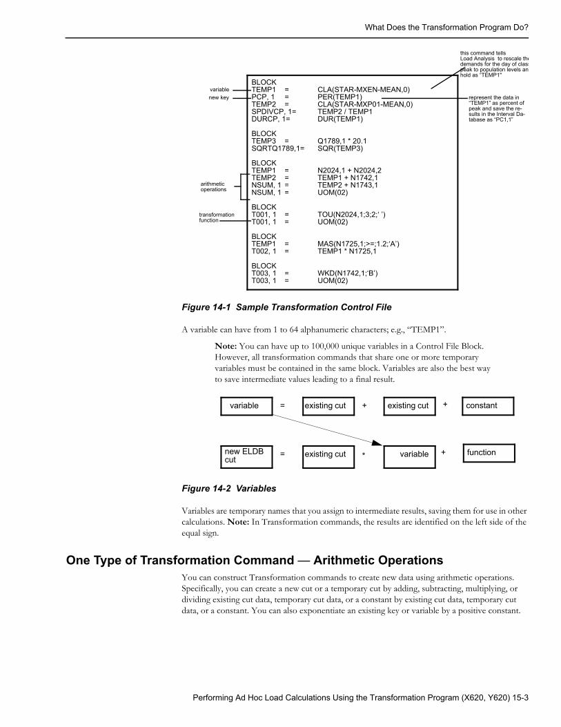
What Does the Transformation Program Do?
Figure 14-1 Sample Transformation Control File
A variable can have from 1 to 64 alphanumeric characters; e.g., “TEMP1”.
Note: You can have up to 100,000 unique variables in a Control File Block. However, all transformation commands that share one or more temporary variables must be contained in the same block. Variables are also the best way to save intermediate values leading to a final result.
Figure 14-2 Variables
Variables are temporary names that you assign to intermediate results, saving them for use in other calculations. Note: In Transformation commands, the results are identified on the left side of the equal sign.
One Type of Transformation Command — Arithmetic OperationsYou can construct Transformation commands to create new data using arithmetic operations. Specifically, you can create a new cut or a temporary cut by adding, subtracting, multiplying, or dividing existing cut data, temporary cut data, or a constant by existing cut data, temporary cut data, or a constant. You can also exponentiate an existing key or variable by a positive constant.
BLOCKTEMP1 = CLA(STAR-MXEN-MEAN,0)PCP, 1 = PER(TEMP1)TEMP2 = CLA(STAR-MXP01-MEAN,0)SPDIVCP, 1= TEMP2 / TEMP1DURCP, 1= DUR(TEMP1)
BLOCKTEMP3 = Q1789,1 * 20.1SQRTQ1789,1= SQR(TEMP3)
BLOCKTEMP1 = N2024,1 + N2024,2TEMP2 = TEMP1 + N1742,1NSUM, 1 = TEMP2 + N1743,1NSUM, 1 = UOM(02)
BLOCKT001, 1 = TOU(N2024,1;3;2;‘ ’)T001, 1 = UOM(02)
BLOCKTEMP1 = MAS(N1725,1;>=;1.2;‘A’)T002, 1 = TEMP1 * N1725,1
BLOCKT003, 1 = WKD(N1742,1;‘B’)T003, 1 = UOM(02)
arithmeticoperations
this command tellsLoad Analysis to rescale thedemands for the day of classpeak to population levels anhold as “TEMP1"
represent the data in“TEMP1” as percent of peak and save the re-sults in the Interval Da-tabase as “PC1,1”
variablenew key
transformationfunction
variable existing cut existing cut= +
new ELDBcut existing cut variable= *
constant
function
+
+
Performing Ad Hoc Load Calculations Using the Transformation Program (X620, Y620) 15-3
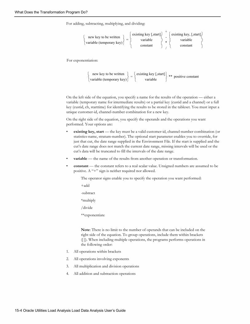
What Does the Transformation Program Do?
For adding, subtracting, multiplying, and dividing:
For exponentiation:
On the left side of the equation, you specify a name for the results of the operation — either a variable (temporary name for intermediate results) or a partial key (custid and a channel) or a full key (custid, ch, starttime) for identifying the results to be stored in the tableset. You must input a unique customer-id, channel-number combination for a new key.
On the right side of the equation, you specify the operands and the operations you want performed. Your options are:
• existing key, start — the key must be a valid customer-id, channel-number combination (or statistics-name, stratum-number). The optional start parameter enables you to override, for just that cut, the date range supplied in the Environment File. If the start is supplied and the cut’s date range does not match the current date range, missing intervals will be used or the cut’s data will be truncated to fill the intervals of the date range.
• variable — the name of the results from another operation or transformation.
• constant — the constant refers to a real scalar value. Unsigned numbers are assumed to be positive. A “+” sign is neither required nor allowed.
The operator signs enable you to specify the operation you want performed:
+add
-subtract
*multiply
/divide
**exponentiate
Note: There is no limit to the number of operands that can be included on the right side of the equation. To group operations, include them within brackets ([ ]). When including multiple operations, the programs performs operations in the following order:
1. All operations within brackets
2. All operations involving exponents
3. All multiplication and division operations
4. All addition and subtraction operations
new key to be writtenvariable (temporary key)
existing key [,start]variableconstant
+-*/
existing key, [,start]variableconstant
=
new key to be writtenvariable (temporary key)
existing key [,start]
variable
** positive constant=
15-4 Oracle Utilities Load Analysis Load Data Analysis User’s Guide
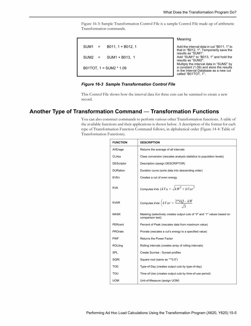
What Does the Transformation Program Do?
Figure 16-3: Sample Transformation Control File is a sample Control File made up of arithmetic Transformation commands.
Figure 16-3 Sample Transformation Control File
This Control File shows how the interval data for three cuts can be summed to create a new record.
Another Type of Transformation Command — Transformation FunctionsYou can also construct commands to perform various other Transformation functions. A table of the available functions and their applications is shown below. A description of the format for each type of Transformation Function Command follows, in alphabetical order (Figure 14-4: Table of Transformation Functions).
SUM1 = B011, 1 + B012, 1
SUM2 = SUM1 + B013, 1
B01TOT, 1 = SUM2 * 1.09
Add the interval data in cut “B011, 1" to that in “B012, 1". Temporarily save the results as “SUM1”.Add “SUM1" to “B013, 1" and hold the results as “SUM2".Multiply the interval data in “SUM2” by a constant (1.09) and store the results in the Interval Database as a new cut called “B01TOT, 1".
Meaning
FUNCTION DESCRIPTION
AVErage Returns the average of all intervals
CLAss Class conversion (rescales analysis statistics to population levels)
DEScriptor Description (assign DESCRIPTOR)
DURation Duration curve (sorts data into descending order)
EVEn Creates a cut of even energy
KVA Computes kVa
KVAR Computes kVar
MASK Masking (selectively creates output cuts of “0" and “1" values based on comparison test)
PERcent Percent of Peak (rescales data from maximum value)
PROrate Prorate (rescales a cut’s energy to a specified value)
PWF Returns the Power Factor
ROLling Rolling intervals (creates array of rolling intervals)
SPL Create Sunrise - Sunset profiles
SQRt Square root (same as “**0.5")
TOD Type-of-Day (creates output cuts by type-of-day)
TOU Time-of-Use (creates output cuts by time-of-use period)
UOM Unit-of-Measure (assign UOM)
kVa kW2 kVar2+=(
kVar 2*kQ kW–3
----------------------------=
Performing Ad Hoc Load Calculations Using the Transformation Program (X620, Y620) 15-5
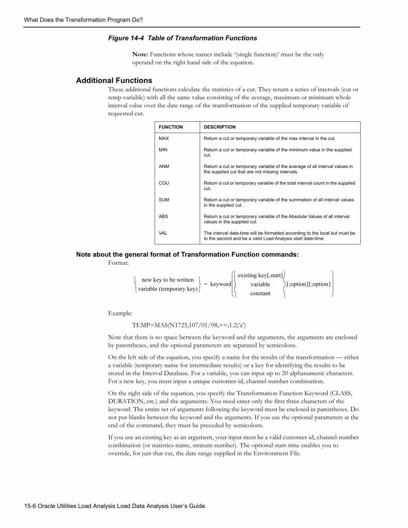
What Does the Transformation Program Do?
Figure 14-4 Table of Transformation Functions
Note: Functions whose names include ‘(single function)’ must be the only operand on the right hand side of the equation.
Additional FunctionsThese additional functions calculate the statistics of a cut. They return a series of intervals (cut or temp variable) with all the same value consisting of the average, maximum or minimum whole interval value over the date range of the transformation of the supplied temporary variable of requested cut.
Note about the general format of Transformation Function commands:Format:
Example:
TEMP=MAS(N1725,107/01/98;>=;1.2;’a’)
Note that there is no space between the keyword and the arguments, the arguments are enclosed by parentheses, and the optional parameters are separated by semicolons.
On the left side of the equation, you specify a name for the results of the transformation — either a variable (temporary name for intermediate results) or a key for identifying the results to be stored in the Interval Database. For a variable, you can input up to 20 alphanumeric characters. For a new key, you must input a unique customer-id, channel-number combination.
On the right side of the equation, you specify the Transformation Function Keyword (CLASS, DURATION, etc.) and the arguments. You need enter only the first three characters of the keyword. The entire set of arguments following the keyword must be enclosed in parentheses. Do not put blanks between the keyword and the arguments. If you use the optional parameters at the end of the command, they must be preceded by semicolons.
If you use an existing key as an argument, your input must be a valid customer-id, channel-number combination (or statistics-name, stratum-number). The optional start-time enables you to override, for just that cut, the date range supplied in the Environment File.
FUNCTION DESCRIPTION
MAX Return a cut or temporary variable of the max interval in the cut.
MIN Return a cut or temporary variable of the minimum value in the supplied cut.
ANM Return a cut or temporary variable of the average of all interval values in the supplied cut that are not missing intervals.
COU Return a cut or temporary variable of the total interval count in the supplied cut.
SUM Return a cut or temporary variable of the summation of all interval values in the supplied cut.
ABS Return a cut or temporary variable of the Absolute Values of all interval values in the supplied cut.
VAL The interval date-time will be formatted according to the local but must be to the second and be a valid Load Analysis start date-time.
new key to be writtenvariable (temporary key)
keywordexisting key[,start]
variableconstant
;option[ ] ;option[ ]
=
15-6 Oracle Utilities Load Analysis Load Data Analysis User’s Guide
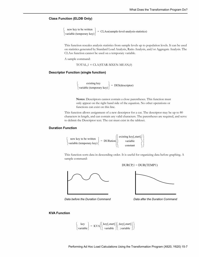
What Does the Transformation Program Do?
Class Function (ELDB Only)
This function rescales analysis statistics from sample levels up to population levels. It can be used on statistics generated by Standard Load Analysis, Ratio Analysis, and/or Aggregate Analysis. The CLAss function cannot be used on a temporary variable.
A sample command:
TOTAL,1 = CLA(STAR-MXEN-MEAN,0)
Descriptor Function (single function)
Notes: Descriptors cannot contain a close parentheses. This function must only appear on the right hand side of the equation. No other operations or functions can exist on this line.
This function allows assignment of a new descriptor for a cut. The descriptor may be up to 80 characters in length, and can contain any valid characters. The parentheses are required, and serve to delimit the Descriptor text. The cut must exist in the tableset.
Duration Function
This function sorts data in descending order. It is useful for organizing data before graphing. A sample command:
DURCP,1 = DUR(TEMP1)
KVA Function
new key to be writtenvariable (temporary key)
CLAss(sample-level-analysis-statistics)=
existing keyvariable (temporary key)
DES(descriptor)=
new key to be writtenvariable (temporary key)
DURationexisting key[,start]
variableconstant
=
Data before the Duration Command Data after the Duration Command
keyvariable
KVAkey[,start]variable
key[,start];
variable;
=
Performing Ad Hoc Load Calculations Using the Transformation Program (X620, Y620) 15-7
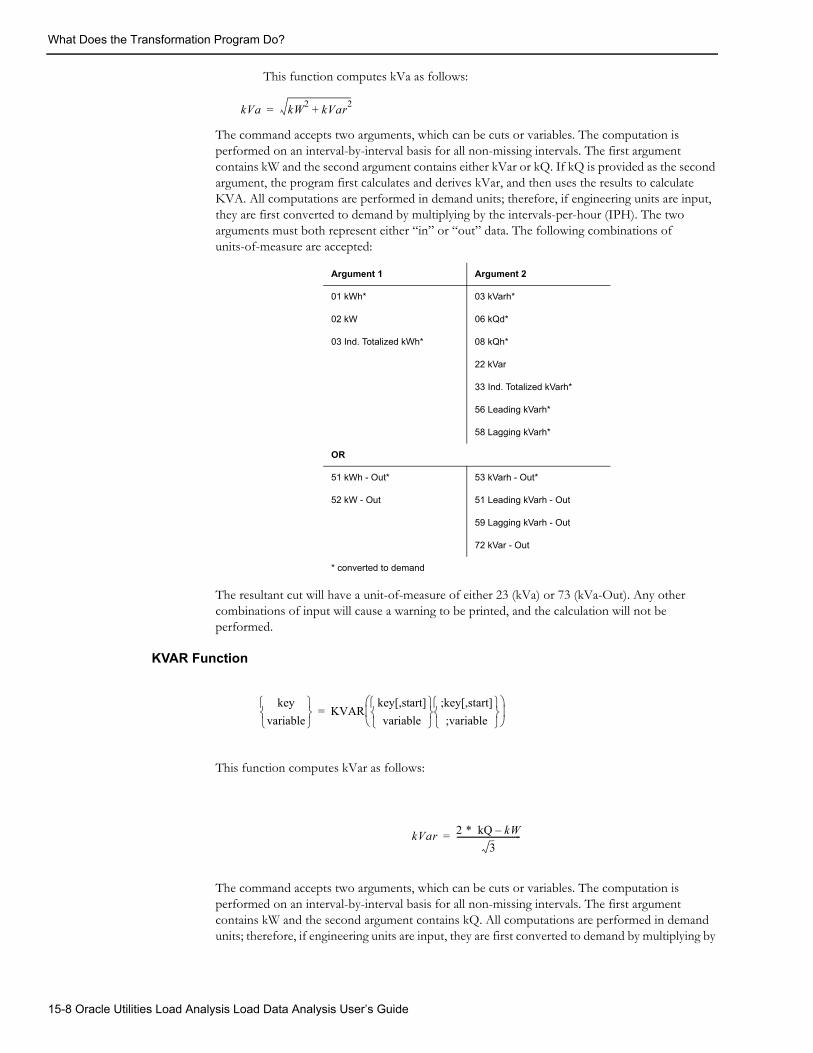
What Does the Transformation Program Do?
This function computes kVa as follows:
The command accepts two arguments, which can be cuts or variables. The computation is performed on an interval-by-interval basis for all non-missing intervals. The first argument contains kW and the second argument contains either kVar or kQ. If kQ is provided as the second argument, the program first calculates and derives kVar, and then uses the results to calculate KVA. All computations are performed in demand units; therefore, if engineering units are input, they are first converted to demand by multiplying by the intervals-per-hour (IPH). The two arguments must both represent either “in” or “out” data. The following combinations of units-of-measure are accepted:
The resultant cut will have a unit-of-measure of either 23 (kVa) or 73 (kVa-Out). Any other combinations of input will cause a warning to be printed, and the calculation will not be performed.
KVAR Function
This function computes kVar as follows:
The command accepts two arguments, which can be cuts or variables. The computation is performed on an interval-by-interval basis for all non-missing intervals. The first argument contains kW and the second argument contains kQ. All computations are performed in demand units; therefore, if engineering units are input, they are first converted to demand by multiplying by
Argument 1 Argument 2
01 kWh* 03 kVarh*
02 kW 06 kQd*
03 Ind. Totalized kWh* 08 kQh*
22 kVar
33 Ind. Totalized kVarh*
56 Leading kVarh*
58 Lagging kVarh*
OR
51 kWh - Out* 53 kVarh - Out*
52 kW - Out 51 Leading kVarh - Out
59 Lagging kVarh - Out
72 kVar - Out
* converted to demand
kVa kW2 kVar2+=
keyvariable
KVARkey[,start]variable
key[,start];
variable;
=
kVar 2 * kQ kW–3
--------------------------------=
15-8 Oracle Utilities Load Analysis Load Data Analysis User’s Guide
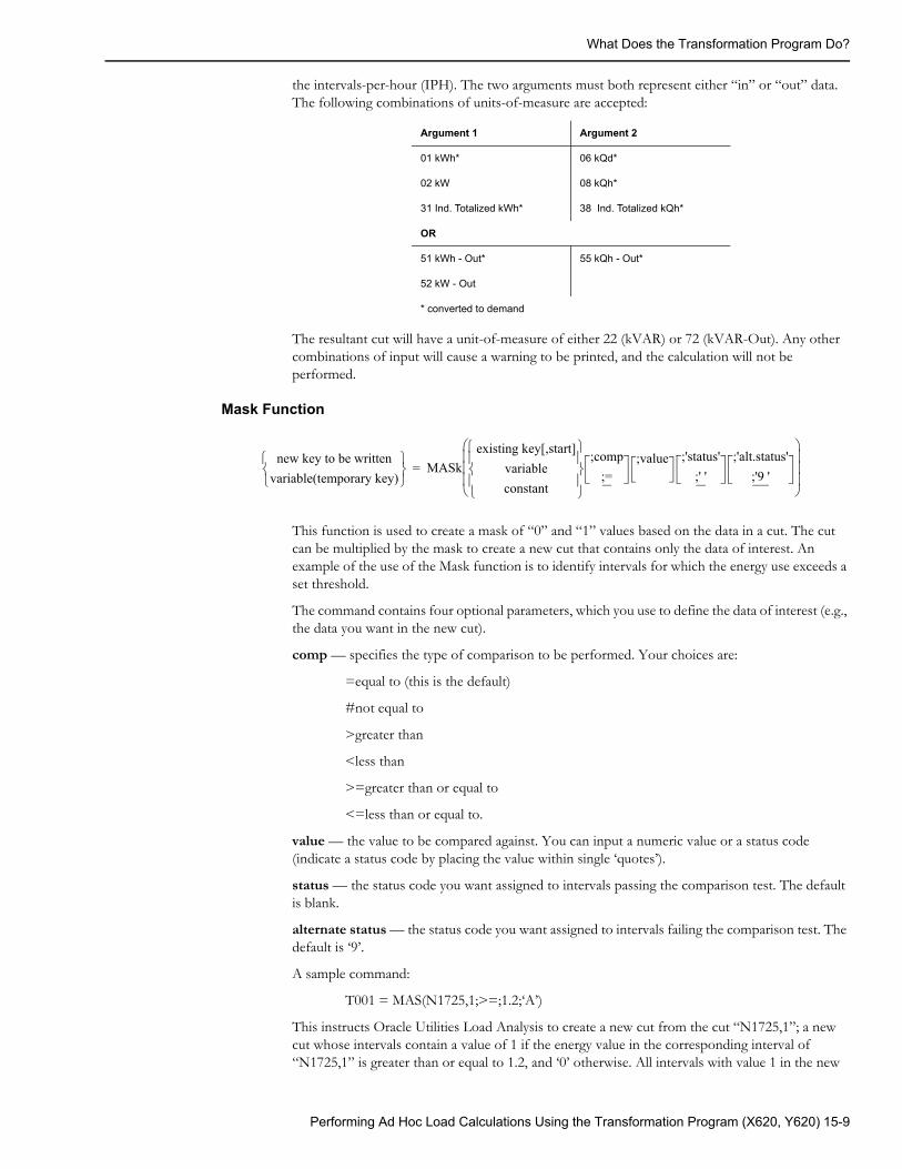
What Does the Transformation Program Do?
the intervals-per-hour (IPH). The two arguments must both represent either “in” or “out” data. The following combinations of units-of-measure are accepted:
The resultant cut will have a unit-of-measure of either 22 (kVAR) or 72 (kVAR-Out). Any other combinations of input will cause a warning to be printed, and the calculation will not be performed.
Mask Function
This function is used to create a mask of “0” and “1” values based on the data in a cut. The cut can be multiplied by the mask to create a new cut that contains only the data of interest. An example of the use of the Mask function is to identify intervals for which the energy use exceeds a set threshold.
The command contains four optional parameters, which you use to define the data of interest (e.g., the data you want in the new cut).
comp — specifies the type of comparison to be performed. Your choices are:
=equal to (this is the default)
#not equal to
>greater than
<less than
>=greater than or equal to
<=less than or equal to.
value — the value to be compared against. You can input a numeric value or a status code (indicate a status code by placing the value within single ‘quotes’).
status — the status code you want assigned to intervals passing the comparison test. The default is blank.
alternate status — the status code you want assigned to intervals failing the comparison test. The default is ‘9’.
A sample command:
T001 = MAS(N1725,1;>=;1.2;‘A’)
This instructs Oracle Utilities Load Analysis to create a new cut from the cut “N1725,1”; a new cut whose intervals contain a value of 1 if the energy value in the corresponding interval of “N1725,1” is greater than or equal to 1.2, and ‘0’ otherwise. All intervals with value 1 in the new
Argument 1 Argument 2
01 kWh* 06 kQd*
02 kW 08 kQh*
31 Ind. Totalized kWh* 38 Ind. Totalized kQh*
OR
51 kWh - Out* 55 kQh - Out*
52 kW - Out
* converted to demand
new key to be writtenvariable(temporary key)
MASkexisting key[,start]
variableconstant
;comp;=
;value
;'status';' '
;'alt.status';'9 '
=
Performing Ad Hoc Load Calculations Using the Transformation Program (X620, Y620) 15-9
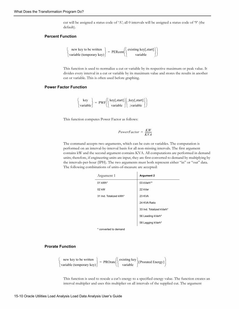
What Does the Transformation Program Do?
cut will be assigned a status code of ‘A’; all 0 intervals will be assigned a status code of ‘9’ (the default).
Percent Function
This function is used to normalize a cut or variable by its respective maximum or peak value. It divides every interval in a cut or variable by its maximum value and stores the results in another cut or variable. This is often used before graphing.
Power Factor Function
This function computes Power Factor as follows:
The command accepts two arguments, which can be cuts or variables. The computation is performed on an interval-by-interval basis for all non-missing intervals. The first argument contains kW and the second argument contains KVA. All computations are performed in demand units; therefore, if engineering units are input, they are first converted to demand by multiplying by the intervals-per-hour (IPH). The two arguments must both represent either “in” or “out” data. The following combinations of units-of-measure are accepted:
Prorate Function
This function is used to rescale a cut’s energy to a specified energy value. The function creates an interval multiplier and uses this multiplier on all intervals of the supplied cut. The argument
new key to be writtenvariable (temporary key)
PERcentexisting key[,start]
variable
=
keyvariable
PWFkey[,start]variable
;key[,start]
;variable
=
Argument 1 Argument 2
01 kWh* 03 kVarh**
02 kW 22 kVar
31 Ind. Totalized kWh* 23 KVA
24 KVA Ratio
33 Ind. Totalized kVarh*
56 Leading kVarh*
58 Lagging kVarh*
* converted to demand
PowerFactor KWKVA------------=
new key to be writtenvariable (temporary key)
PROrateexisting key
variable
Prorated Energy[ ]
=
15-10 Oracle Utilities Load Analysis Load Data Analysis User’s Guide
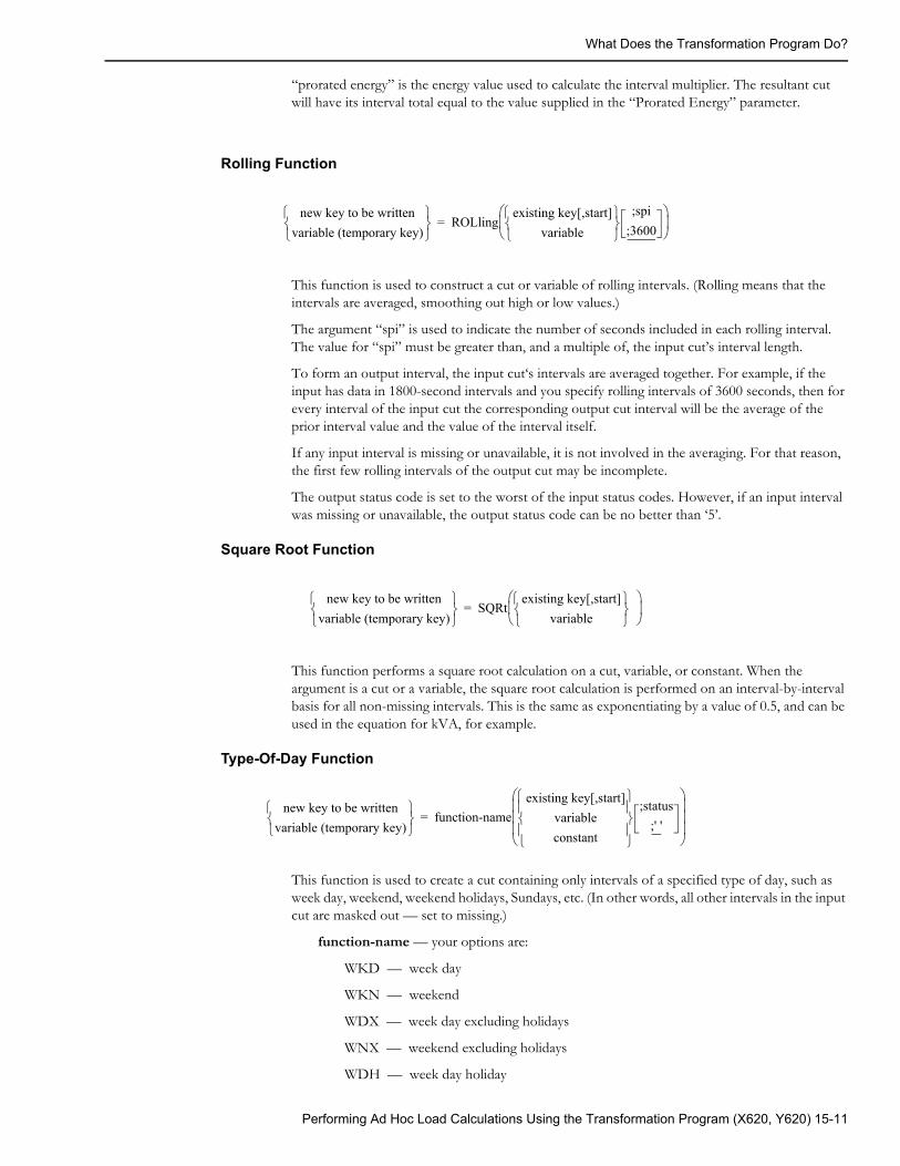
What Does the Transformation Program Do?
“prorated energy” is the energy value used to calculate the interval multiplier. The resultant cut will have its interval total equal to the value supplied in the “Prorated Energy” parameter.
Rolling Function
This function is used to construct a cut or variable of rolling intervals. (Rolling means that the intervals are averaged, smoothing out high or low values.)
The argument “spi” is used to indicate the number of seconds included in each rolling interval. The value for “spi” must be greater than, and a multiple of, the input cut’s interval length.
To form an output interval, the input cut‘s intervals are averaged together. For example, if the input has data in 1800-second intervals and you specify rolling intervals of 3600 seconds, then for every interval of the input cut the corresponding output cut interval will be the average of the prior interval value and the value of the interval itself.
If any input interval is missing or unavailable, it is not involved in the averaging. For that reason, the first few rolling intervals of the output cut may be incomplete.
The output status code is set to the worst of the input status codes. However, if an input interval was missing or unavailable, the output status code can be no better than ‘5’.
Square Root Function
This function performs a square root calculation on a cut, variable, or constant. When the argument is a cut or a variable, the square root calculation is performed on an interval-by-interval basis for all non-missing intervals. This is the same as exponentiating by a value of 0.5, and can be used in the equation for kVA, for example.
Type-Of-Day Function
This function is used to create a cut containing only intervals of a specified type of day, such as week day, weekend, weekend holidays, Sundays, etc. (In other words, all other intervals in the input cut are masked out — set to missing.)
function-name — your options are:
WKD — week day
WKN — weekend
WDX — week day excluding holidays
WNX — weekend excluding holidays
WDH — week day holiday
new key to be writtenvariable (temporary key)
ROLlingexisting key[,start]
variable ;spi
;3600
=
new key to be writtenvariable (temporary key)
SQRtexisting key[,start]
variable
=
new key to be writtenvariable (temporary key)
function-nameexisting key[,start]
variableconstant
;status;' '
=
Performing Ad Hoc Load Calculations Using the Transformation Program (X620, Y620) 15-11
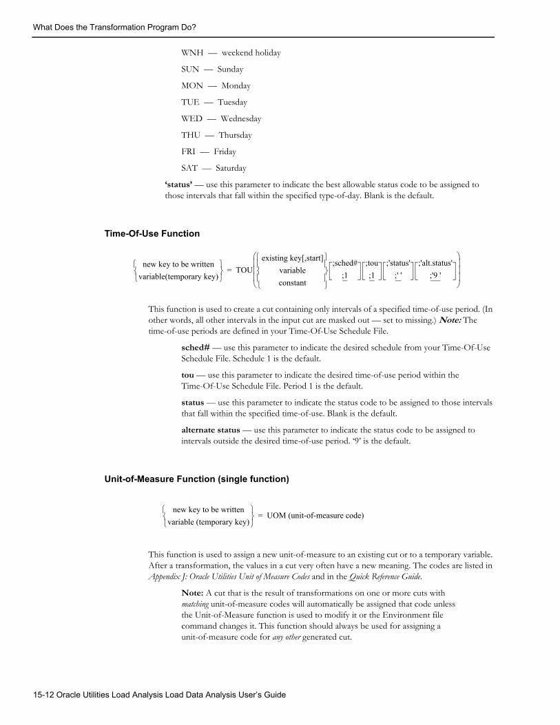
What Does the Transformation Program Do?
WNH — weekend holiday
SUN — Sunday
MON — Monday
TUE — Tuesday
WED — Wednesday
THU — Thursday
FRI — Friday
SAT — Saturday
‘status’ — use this parameter to indicate the best allowable status code to be assigned to those intervals that fall within the specified type-of-day. Blank is the default.
Time-Of-Use Function
This function is used to create a cut containing only intervals of a specified time-of-use period. (In other words, all other intervals in the input cut are masked out — set to missing.) Note: The time-of-use periods are defined in your Time-Of-Use Schedule File.
sched# — use this parameter to indicate the desired schedule from your Time-Of-Use Schedule File. Schedule 1 is the default.
tou — use this parameter to indicate the desired time-of-use period within the Time-Of-Use Schedule File. Period 1 is the default.
status — use this parameter to indicate the status code to be assigned to those intervals that fall within the specified time-of-use. Blank is the default.
alternate status — use this parameter to indicate the status code to be assigned to intervals outside the desired time-of-use period. ‘9’ is the default.
Unit-of-Measure Function (single function)
This function is used to assign a new unit-of-measure to an existing cut or to a temporary variable. After a transformation, the values in a cut very often have a new meaning. The codes are listed in Appendix J: Oracle Utilities Unit of Measure Codes and in the Quick Reference Guide.
Note: A cut that is the result of transformations on one or more cuts with matching unit-of-measure codes will automatically be assigned that code unless the Unit-of-Measure function is used to modify it or the Environment file command changes it. This function should always be used for assigning a unit-of-measure code for any other generated cut.
new key to be writtenvariable(temporary key)
TOUexisting key[,start]
variableconstant
;sched#;1
;tou;1
;'status';' '
;'alt.status';'9 '
=
new key to be writtenvariable (temporary key)
UOM (unit-of-measure code)=
15-12 Oracle Utilities Load Analysis Load Data Analysis User’s Guide
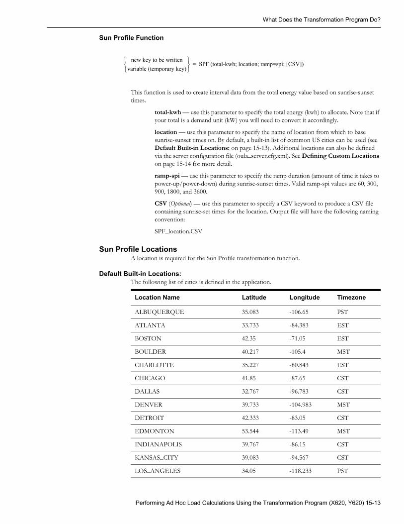
What Does the Transformation Program Do?
Sun Profile Function
This function is used to create interval data from the total energy value based on sunrise-sunset times.
total-kwh — use this parameter to specify the total energy (kwh) to allocate. Note that if your total is a demand unit (kW) you will need to convert it accordingly.
location — use this parameter to specify the name of location from which to base sunrise-sunset times on. By default, a built-in list of common US cities can be used (see Default Built-in Locations: on page 15-13). Additional locations can also be defined via the server configuration file (oula_server.cfg.xml). See Defining Custom Locations on page 15-14 for more detail.
ramp-spi — use this parameter to specify the ramp duration (amount of time it takes to power-up/power-down) during sunrise-sunset times. Valid ramp-spi values are 60, 300, 900, 1800, and 3600.
CSV (Optional) — use this parameter to specify a CSV keyword to produce a CSV file containing sunrise-set times for the location. Output file will have the following naming convention:
SPF_location.CSV
Sun Profile LocationsA location is required for the Sun Profile transformation function.
Default Built-in Locations:The following list of cities is defined in the application.
new key to be writtenvariable (temporary key)
SPF (total-kwh; location; ramp=spi; [CSV])=
Location Name Latitude Longitude Timezone
ALBUQUERQUE 35.083 -106.65 PST
ATLANTA 33.733 -84.383 EST
BOSTON 42.35 -71.05 EST
BOULDER 40.217 -105.4 MST
CHARLOTTE 35.227 -80.843 EST
CHICAGO 41.85 -87.65 CST
DALLAS 32.767 -96.783 CST
DENVER 39.733 -104.983 MST
DETROIT 42.333 -83.05 CST
EDMONTON 53.544 -113.49 MST
INDIANAPOLIS 39.767 -86.15 CST
KANSAS_CITY 39.083 -94.567 CST
LOS_ANGELES 34.05 -118.233 PST
Performing Ad Hoc Load Calculations Using the Transformation Program (X620, Y620) 15-13
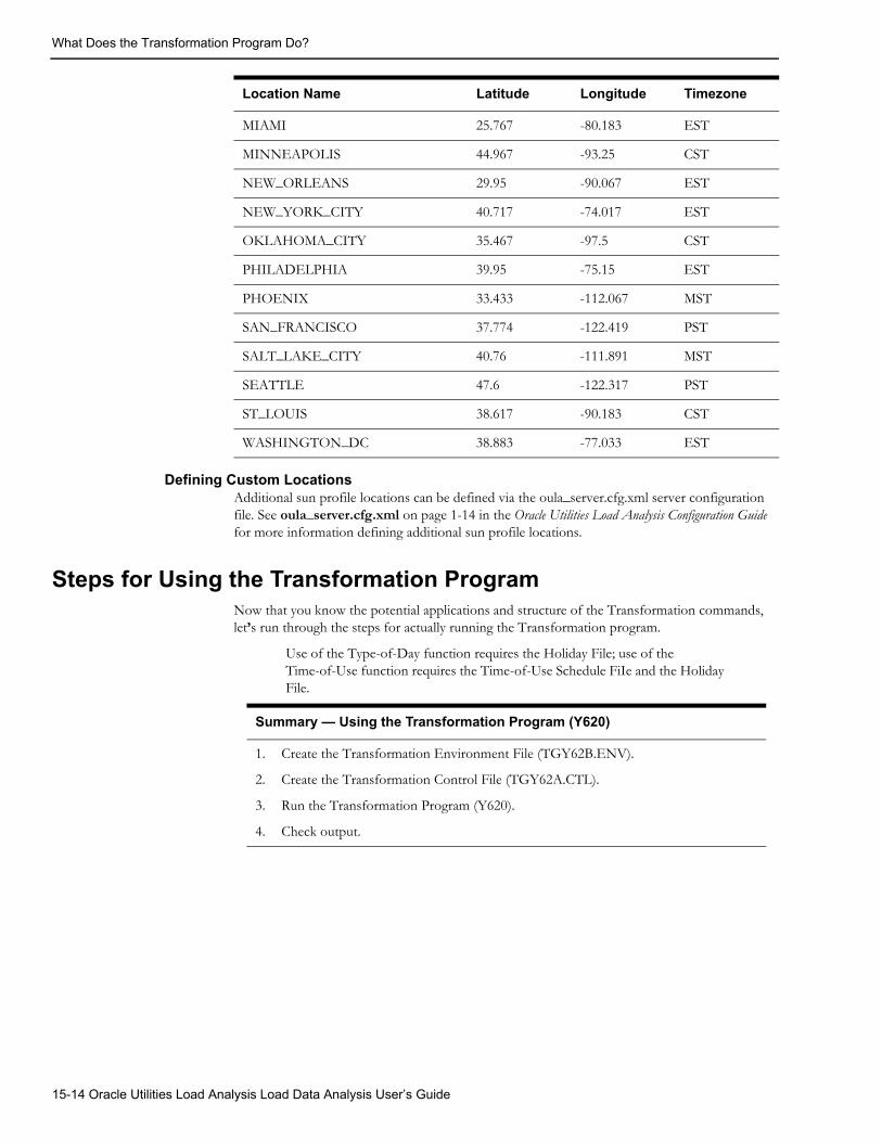
What Does the Transformation Program Do?
Defining Custom LocationsAdditional sun profile locations can be defined via the oula_server.cfg.xml server configuration file. See oula_server.cfg.xml on page 1-14 in the Oracle Utilities Load Analysis Configuration Guide for more information defining additional sun profile locations.
Steps for Using the Transformation ProgramNow that you know the potential applications and structure of the Transformation commands, let’s run through the steps for actually running the Transformation program.
Use of the Type-of-Day function requires the Holiday File; use of the Time-of-Use function requires the Time-of-Use Schedule FiIe and the Holiday File.
MIAMI 25.767 -80.183 EST
MINNEAPOLIS 44.967 -93.25 CST
NEW_ORLEANS 29.95 -90.067 EST
NEW_YORK_CITY 40.717 -74.017 EST
OKLAHOMA_CITY 35.467 -97.5 CST
PHILADELPHIA 39.95 -75.15 EST
PHOENIX 33.433 -112.067 MST
SAN_FRANCISCO 37.774 -122.419 PST
SALT_LAKE_CITY 40.76 -111.891 MST
SEATTLE 47.6 -122.317 PST
ST_LOUIS 38.617 -90.183 CST
WASHINGTON_DC 38.883 -77.033 EST
Location Name Latitude Longitude Timezone
Summary — Using the Transformation Program (Y620)
1. Create the Transformation Environment File (TGY62B.ENV).
2. Create the Transformation Control File (TGY62A.CTL).
3. Run the Transformation Program (Y620).
4. Check output.
15-14 Oracle Utilities Load Analysis Load Data Analysis User’s Guide
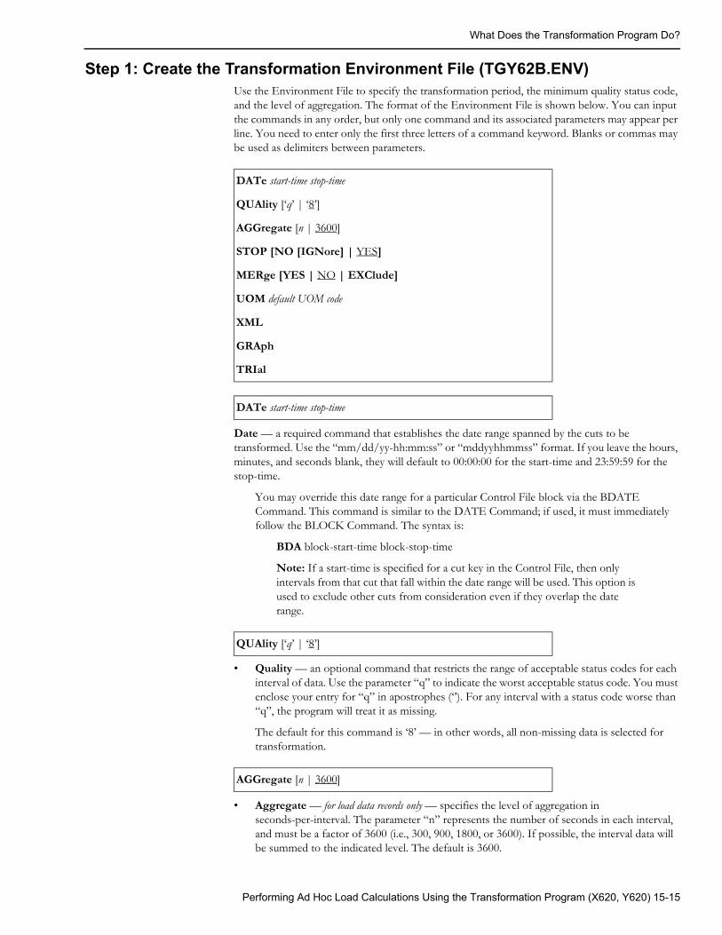
What Does the Transformation Program Do?
Step 1: Create the Transformation Environment File (TGY62B.ENV)Use the Environment File to specify the transformation period, the minimum quality status code, and the level of aggregation. The format of the Environment File is shown below. You can input the commands in any order, but only one command and its associated parameters may appear per line. You need to enter only the first three letters of a command keyword. Blanks or commas may be used as delimiters between parameters.
Date — a required command that establishes the date range spanned by the cuts to be transformed. Use the “mm/dd/yy-hh:mm:ss” or “mddyyhhmmss” format. If you leave the hours, minutes, and seconds blank, they will default to 00:00:00 for the start-time and 23:59:59 for the stop-time.
You may override this date range for a particular Control File block via the BDATE Command. This command is similar to the DATE Command; if used, it must immediately follow the BLOCK Command. The syntax is:
BDA block-start-time block-stop-time
Note: If a start-time is specified for a cut key in the Control File, then only intervals from that cut that fall within the date range will be used. This option is used to exclude other cuts from consideration even if they overlap the date range.
• Quality — an optional command that restricts the range of acceptable status codes for each interval of data. Use the parameter “q” to indicate the worst acceptable status code. You must enclose your entry for “q” in apostrophes (‘’). For any interval with a status code worse than “q”, the program will treat it as missing.
The default for this command is ‘8’ — in other words, all non-missing data is selected for transformation.
• Aggregate — for load data records only — specifies the level of aggregation in seconds-per-interval. The parameter “n” represents the number of seconds in each interval, and must be a factor of 3600 (i.e., 300, 900, 1800, or 3600). If possible, the interval data will be summed to the indicated level. The default is 3600.
DATe start-time stop-time
QUAlity [‘q’ | ‘8’]
AGGregate [n | 3600]
STOP [NO [IGNore] | YES]
MERge [YES | NO | EXClude]
UOM default UOM code
XML
GRAph
TRIal
DATe start-time stop-time
QUAlity [‘q’ | ‘8’]
AGGregate [n | 3600]
Performing Ad Hoc Load Calculations Using the Transformation Program (X620, Y620) 15-15
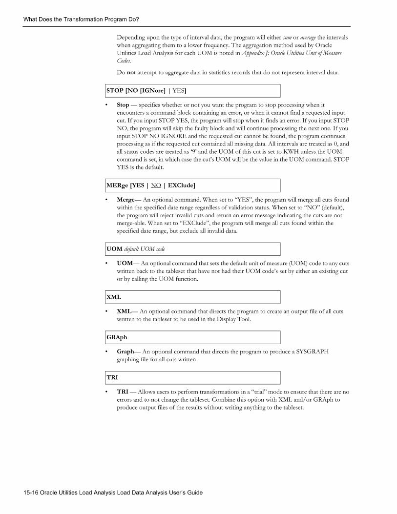
What Does the Transformation Program Do?
Depending upon the type of interval data, the program will either sum or average the intervals when aggregating them to a lower frequency. The aggregation method used by Oracle Utilities Load Analysis for each UOM is noted in Appendix J: Oracle Utilities Unit of Measure Codes.
Do not attempt to aggregate data in statistics records that do not represent interval data.
• Stop — specifies whether or not you want the program to stop processing when it encounters a command block containing an error, or when it cannot find a requested input cut. If you input STOP YES, the program will stop when it finds an error. If you input STOP NO, the program will skip the faulty block and will continue processing the next one. If you input STOP NO IGNORE and the requested cut cannot be found, the program continues processing as if the requested cut contained all missing data. All intervals are treated as 0, and all status codes are treated as ‘9’ and the UOM of this cut is set to KWH unless the UOM command is set, in which case the cut’s UOM will be the value in the UOM command. STOP YES is the default.
• Merge— An optional command. When set to “YES”, the program will merge all cuts found within the specified date range regardless of validation status. When set to “NO” (default), the program will reject invalid cuts and return an error message indicating the cuts are not merge-able. When set to “EXClude”, the program will merge all cuts found within the specified date range, but exclude all invalid data.
• UOM— An optional command that sets the default unit of measure (UOM) code to any cuts written back to the tableset that have not had their UOM code’s set by either an existing cut or by calling the UOM function.
• XML— An optional command that directs the program to create an output file of all cuts written to the tableset to be used in the Display Tool.
• Graph— An optional command that directs the program to produce a SYSGRAPH graphing file for all cuts written
• TRI — Allows users to perform transformations in a “trial” mode to ensure that there are no errors and to not change the tableset. Combine this option with XML and/or GRAph to produce output files of the results without writing anything to the tableset.
STOP [NO [IGNore] | YES]
MERge [YES | NO | EXClude]
UOM default UOM code
XML
GRAph
TRI
15-16 Oracle Utilities Load Analysis Load Data Analysis User’s Guide
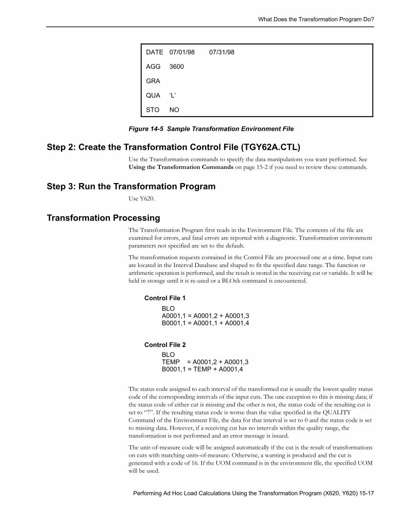
What Does the Transformation Program Do?
Figure 14-5 Sample Transformation Environment File
Step 2: Create the Transformation Control File (TGY62A.CTL)Use the Transformation commands to specify the data manipulations you want performed. See Using the Transformation Commands on page 15-2 if you need to review these commands.
Step 3: Run the Transformation ProgramUse Y620.
Transformation ProcessingThe Transformation Program first reads in the Environment File. The contents of the file are examined for errors, and fatal errors are reported with a diagnostic. Transformation environment parameters not specified are set to the default.
The transformation requests contained in the Control File are processed one at a time. Input cuts are located in the Interval Database and shaped to fit the specified date range. The function or arithmetic operation is performed, and the result is stored in the receiving cut or variable. It will be held in storage until it is re-used or a BLOck command is encountered.
The status code assigned to each interval of the transformed cut is usually the lowest quality status code of the corresponding intervals of the input cuts. The one exception to this is missing data; if the status code of either cut is missing and the other is not, the status code of the resulting cut is set to “7”. If the resulting status code is worse than the value specified in the QUALITY Command of the Environment File, the data for that interval is set to 0 and the status code is set to missing data. However, if a receiving cut has no intervals within the quality range, the transformation is not performed and an error message is issued.
The unit-of-measure code will be assigned automatically if the cut is the result of transformations on cuts with matching units-of-measure. Otherwise, a warning is produced and the cut is generated with a code of 16. If the UOM command is in the environment file, the specified UOM will be used.
DATE 07/01/98 07/31/98
AGG 3600
GRA
QUA ‘L’
STO NO
BLOA0001,1 = A0001,2 + A0001,3B0001,1 = A0001,1 + A0001,4
Control File 1
BLOTEMP = A0001,2 + A0001,3B0001,1 = TEMP + A0001,4
Control File 2
Performing Ad Hoc Load Calculations Using the Transformation Program (X620, Y620) 15-17
What Does the Transformation Program Do?
The transformation period can span a varying number of days. This includes periods spanning a month boundary (e.g., 06/15/98 to 07/15/98), short periods (e.g., 07/02/98 to 07/05/98), and periods longer than a calendar month (e.g., 06/15/98 to 08/30/98). If the optional start-time parameter is used, the transformations begin using the first interval of the cut and continue for the same number of intervals as there are intervals corresponding to the date range.
If a cut produced by a transformation is given the same key as a cut already residing on the Interval Database, the Interval Database cut is automatically overwritten.
If the STOP Command in the Environment File was set to “YES” and an error is found in a transformation request, or if a requested input cut is not found, all transformation processing will stop and a Return Code of 10 will be produced. If the STOP Command was set to “NO” and an error is found, the remaining Transformation commands in the block containing the error will not be performed, and processing will continue with the next BLOCK Command.
15-18 Oracle Utilities Load Analysis Load Data Analysis User’s Guide
Chapter 16Making Oracle Utilities Load Analysis Data
Available for External Applications (X710, Y710,X720, X740, Y720, Y740, Y780)
Despite Oracle Utilities Load Analysis’s extensive capabilities, there may be times when you want to apply other programs to your Oracle Utilities Load Analysis data — such as user-written programs, other utility software, or spreadsheet packages. This chapter describes two Oracle Utilities Load Analysis programs you can use to make your data available for external applications:
• Direct Output Program
• Steps for Using the Direct Output Program
• The Direct Output Format (.INP)
• Daily Output Format
• Statistical Package Interface Program (X710, Y710)
• Steps for Using the Statistical Package Interface Program (X710, Y710)
• Statistic Extraction Program (Y780)
• Steps for Using the Statistic Extraction Program (Y780)
Making Oracle Utilities Load Analysis Data Available for External Applications (X710, Y710, X720, X740, Y720, Y740, Y780) 16-1
There are three choices for making Oracle Utilities Load Analysis data available for ad hoc analysis and other external application programs:
I - Direct Output Program — similar to the Direct Output Program, but the output can be in one of several formats, including:
• LSE: The Oracle Utilities Enhanced Input/Output interval data format.
• CSV: comma-separated values format.
• DAI: The Daily Energy format. See the DAIly command on page 16-8 for more information about this format.
• INP: The Oracle Utilities Load Analysis standard pulse format. See The Direct Output Format (.INP) on page 16-13 for more information about this format.
• XML: “compact” XML format (see the Oracle Utilities Energy Information Platform Configuration Guide for more information about this format).
• GRAph: Produces the graphing file, SYSGRAPH.HTM for graphical display of all cuts extracted.
II - Statistical Package Interface Program — reformats load data contained in CLDB or ELDB cuts into a matrix format with a matching file of header information that can be read by external applications.
III - Statistic Extraction Program — extracts specified cuts or statistics over multiple analysis rate classes over multiple analysis periods into a CSV file that may be imported into a spreadsheet or reporting tool.
These programs are discussed in detail in the remainder of this chapter.
Note: The current CSV format is time-aligned which means all cuts extracted will be aligned to a single common date/time column. For example, if a cut begins at a later date/time, data for that cut will begin at a later row. Unlike the older format, this newer one includes status codes.
Should for any reason, users prefer the older CSV format, they can do so by adding the following GLB setting:
CSVFORMAT OLD
16-2 Oracle Utilities Load Analysis Load Data Analysis User’s Guide
Direct Output Program
Direct Output ProgramThe Direct Output programs are X720 (CLDB), Y720 (ELDB), X740 (ALDB), and Y740 (SLDB). All of these are accessible from the Direct Output submit screen.
These programs are used to output load data and/or statistics from any of the major Oracle Utilities Load Analysis tablesets (ELDB, SLDB, CLDB, ALDB) in a format that is compatible with most computer languages, including Java and VBS. The data is thus available for use with user-written or other application programs. The output format is also suitable for transmission via the Internet.
With Direct Output, you can output individual cuts, cut series, or subsets of a cut series. There are no limits to the number of cuts; in fact, you can easily output the entire contents of a tableset.
Note: Cuts that make use of the Enhanced Format specifications (i.e., custid length > 20, etc.) are not eligible for extraction via .INP format.
The programs transform the data into a simple sequential format and write it out to a sequential data set. Interval data is recorded as “energy.” You can keep status codes with the interval data.
Oracle Utilities Load Analysis includes a companion program called Direct Input (TGX110 - see Oracle Utilities Load Analysis Load Data Management User’s Guide) that makes it possible to manipulate data outside of Oracle Utilities Load Analysis and return it for storage to one of the Oracle Utilities Load Analysis tablesets — e.g., when you want to add transmission and distribution losses to class profiles and keep the results in the SLDB.
Note: The X720 and Y720 program supports embedded SQL commands. See Querying the Database with Embedded Query Statements on page 4-7 for more information. The programs also supports pre-process key generator. See Using the Key Generator Preprocessor in a Control File on page 4-4 for more information.
Making Oracle Utilities Load Analysis Data Available for External Applications (X710, Y710, X720, X740, Y720, Y740, Y780) 16-3
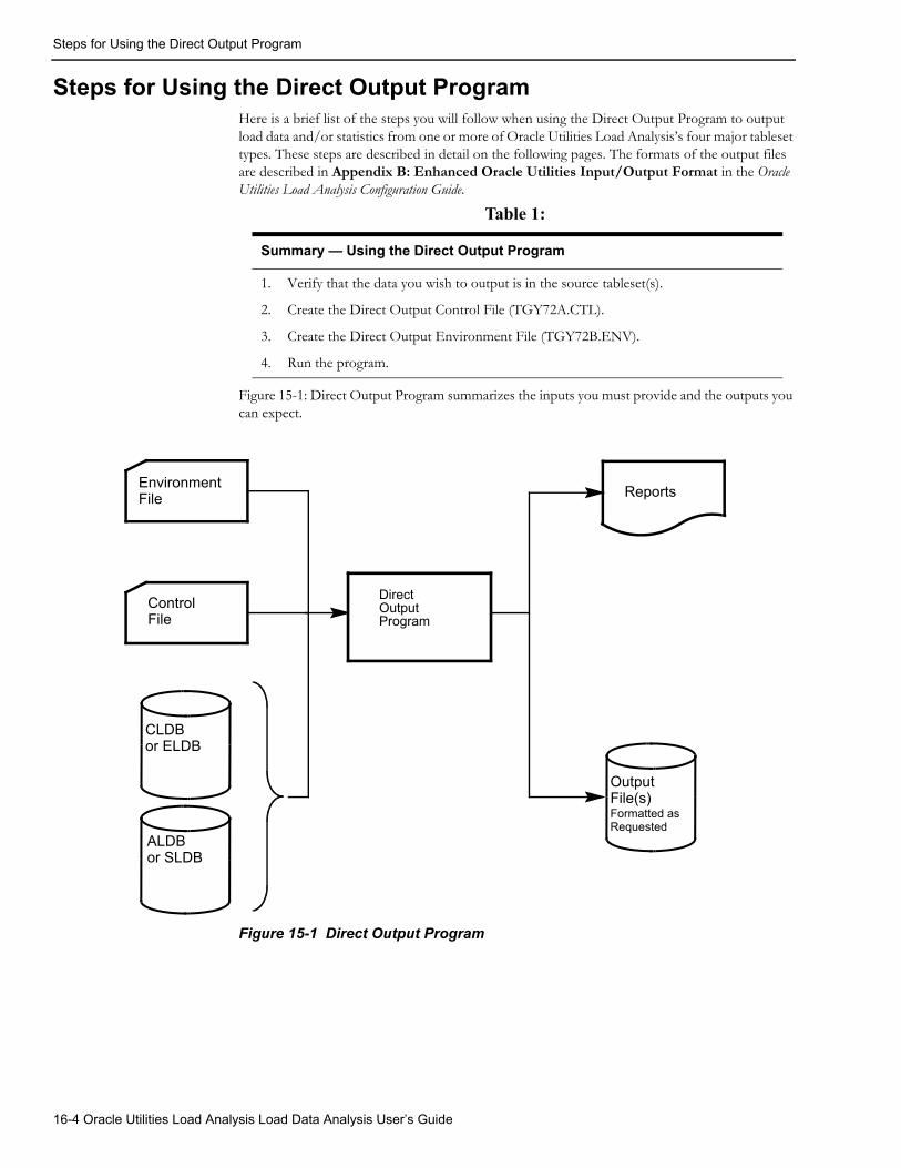
Steps for Using the Direct Output Program
Steps for Using the Direct Output ProgramHere is a brief list of the steps you will follow when using the Direct Output Program to output load data and/or statistics from one or more of Oracle Utilities Load Analysis’s four major tableset types. These steps are described in detail on the following pages. The formats of the output files are described in Appendix B: Enhanced Oracle Utilities Input/Output Format in the Oracle Utilities Load Analysis Configuration Guide.
Figure 15-1: Direct Output Program summarizes the inputs you must provide and the outputs you can expect.
Figure 15-1 Direct Output Program
Table 1:
Summary — Using the Direct Output Program
1. Verify that the data you wish to output is in the source tableset(s).
2. Create the Direct Output Control File (TGY72A.CTL).
3. Create the Direct Output Environment File (TGY72B.ENV).
4. Run the program.
DirectOutputProgram
ReportsEnvironmentFile
ControlFile
CLDB or ELDB
Output File(s)Formatted as Requested
ALDBor SLDB
16-4 Oracle Utilities Load Analysis Load Data Analysis User’s Guide
Steps for Using the Direct Output Program
Step 1: Verify that the Data you wish to Output is in the Source Tableset(s)In the Environment File, specify which of the major Oracle Utilities Load Analysis tablesets you want to use as the data source — CLDB, ALDB, ELDB, or SLDB. You can specify any one of the tablesets or a combination (either the CLDB/ALDB, or the ELDB/SLDB). If you specify CLDB/ALDB and a key in your Control File has data in both tablesets, the cut will be read from the CLDB. Similarly, if you specify ELDB/SLDB and a key in your Control File has data in both tablesets, the cut will be read from the ELDB.
Note: Not all Control File and Environment File options are available for all tablesets. These restrictions are explained in the following pages and summarized in Table 16-2.
Step 2: Create the Direct Output Control FileThe Control File contains the keys of load data records and/or statistics that you want to output, along with some optional parameters. The format for each Control File record is shown in the box below.
You can include any number of records in a Control File.
• customer-id, channel (required) — enter the Oracle Utilities Load Analysis customer-id, channel for load data records, or the statistic-id, stratum for statistics.
• start-time (optional) — supply the cut’s start-time if you want to output interval data for the recording period of the cut. If you want instead to output interval data for a cut series (merged cuts) over a different date range, omit the start-time here and specify the date range using the Date Command in the Environment File.
If you supply a cut's start-time in the Control File and a Date Command in the Environment File, then only that data in the cut specified in the Control File that falls within the period indicated in the Date Command will be extracted and written to the output file. The Date Command will determine the start time and stop-time of the output data, and any intervals within that period that cannot be filled from the specified cut will be written as missing intervals (status code = '9', value = 0). If there are no intervals in the specified cut for the period indicated in the Date Command, no output will be written, and a message indicating this will be written in the Execution Log.
If you do not supply a Date Command in the Environment File, you must supply a start-time for every customer-id, channel record specified.
Note: If you wish to output invalid data from the CLDB, you must specify the start-time of the cut. (Invalid data cannot be merged into a cut series. You can only output it as individual cuts.)
• stop-time (optional) — supply the cut’s stop time if you want override the stop time specified in the Date command in the Environment file for the cut.
• Active/Inactive (optional) — in the case of an edited cut, this parameter specifies whether edited data (ACTIVE) or original data (INACTIVE) should be written out. The default is ACTIVE. See Chapter 6 for details about the Load Data Editor.
Note: INACTIVE may be specified only for the CLDB (inactive records cannot be retrieved from the ALDB, SLDB, or ELDB). If you specify INACTIVE and no inactive records are available on the CLDB, the program will issue an error message.
• Class (optional) — this parameter is used to scale analysis statistics (sample mean and variance of the mean) to the class level (class total and variance). If you do not specify this option, the analysis statistics will be reported at the level at which they were originally written.
customer-id, channel [,start-time][,stop-time][,INActive | ,ACTive] [,CLAss]
Making Oracle Utilities Load Analysis Data Available for External Applications (X710, Y710, X720, X740, Y720, Y740, Y780) 16-5
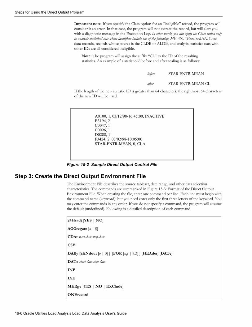
Steps for Using the Direct Output Program
Important note: If you specify the Class option for an “ineligible” record, the program will consider it an error. In that case, the program will not extract the record, but will alert you with a diagnostic message in the Execution Log. In other words, you can apply the Class option only to analysis statistical cuts whose identifiers include one of the following: MEAN, SExx, xMEN. Load data records, records whose source is the CLDB or ALDB, and analysis statistics cuts with other IDs are all considered ineligible.
Note: The program will assign the suffix “CL” to the ID of the resulting statistics. An example of a statistic-id before and after scaling is as follows:
If the length of the new statistic ID is greater than 64 characters, the rightmost 64 characters of the new ID will be used.
Figure 15-2 Sample Direct Output Control File
Step 3: Create the Direct Output Environment FileThe Environment File describes the source tableset, date range, and other data selection characteristics. The commands are summarized in Figure 15-3: Format of the Direct Output Environment File. When creating the file, enter one command per line. Each line must begin with the command name (keyword); but you need enter only the first three letters of the keyword. You may enter the commands in any order. If you do not specify a command, the program will assume the default (underlined). Following is a detailed description of each command
before
after
STAR-ENTR-MEAN
STAR-ENTR-MEAN-CL
A0100, 1, 03/12/98-16:45:00, INACTIVEB3194, 2C0047, 1C0096, 1D0288, 1F3424, 2, 03/02/98-10:05:00STAR-ENTR-MEAN, 0, CLA
24Hradj [YES | NO]
AGGregate [n | 0]
CDAt start-date stop-date
CSV
DAIly [SENdout [h | 0] ] [FOR [x.y | 7.3] ] [HEAder] [DATe]
DATe start-date stop-date
INP
LSE
MERge [YES | NO | EXClude]
ONErecord
16-6 Oracle Utilities Load Analysis Load Data Analysis User’s Guide
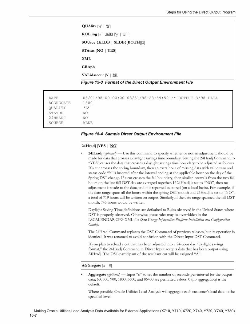
Steps for Using the Direct Output Program
Figure 15-3 Format of the Direct Output Environment File .
Figure 15-4 Sample Direct Output Environment File
• 24Hradj (optional) — Use this command to specify whether or not an adjustment should be made for data that crosses a daylight savings time boundary. Setting the 24Hradj Command to “YES” causes the data that crosses a daylight savings time boundary to be adjusted as follows. If a cut crosses the spring boundary, then an extra hour of missing data with value zero and status code “9” is inserted after the interval ending at the applicable hour on the day of the Spring DST change. If a cut crosses the fall boundary, then similar intervals from the two fall hours on the last full DST day are averaged together. If 24Hradj is set to “NO”, then no adjustment is made to the data, and it is reported as stored (on a local basis). For example, if the date range spans all the hours within the spring DST month and 24Hradj is set to “NO”, a total of 719 hours will be written on output. Similarly, if the date range spanned the fall DST month, 745 hours would be written.
Daylight Saving Time definitions are defaulted to Rules observed in the United States where DST is properly observed. Otherwise, these rules may be overridden in the LSCALENDAR.CFG XML file (See Energy Information Platform Installation and Configuration Guide).
The 24Hradj Command replaces the DST Command of previous releases, but its operation is identical. It was renamed to avoid confusion with the Direct Input DST Command.
If you plan to reload a cut that has been adjusted into a 24-hour day “daylight savings format,” the 24Hradj Command in Direct Input accepts data that has been output using 24Hradj. The DST-participant of the resultant cut will be assigned “A”.
• Aggregate (optional) — Input “n” to set the number of seconds-per-interval for the output data; 60, 300, 900, 1800, 3600, and 86400 are permitted values. 0 (no aggregation) is the default.
Where possible, Oracle Utilities Load Analysis will aggregate each customer’s load data to the specified level.
QUAlity [‘q’ | ‘8’]
ROLling [n | 3600 [‘q’ | ‘8’] ]
SOUrce {ELDB | SLDB}[BOTH][2]
STAtus [NO | YES]
XML
GRAph
VALidatecut [Y | N]
DATEAGGREGATEQUALITYSTATUS24HRADJSOURCE
03/01/98-00:00:00 03/31/98-23:59:59 /* OUTPUT 3/98 DATA1800‘L’NONOALDB
24Hradj [YES | NO]
AGGregate [n | 0]
Making Oracle Utilities Load Analysis Data Available for External Applications (X710, Y710, X720, X740, Y720, Y740, Y780) 16-7
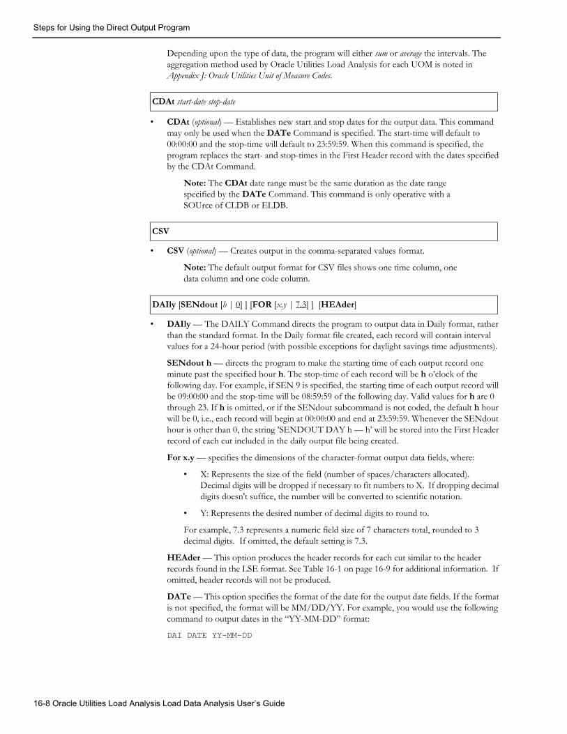
Steps for Using the Direct Output Program
Depending upon the type of data, the program will either sum or average the intervals. The aggregation method used by Oracle Utilities Load Analysis for each UOM is noted in Appendix J: Oracle Utilities Unit of Measure Codes.
• CDAt (optional) — Establishes new start and stop dates for the output data. This command may only be used when the DATe Command is specified. The start-time will default to 00:00:00 and the stop-time will default to 23:59:59. When this command is specified, the program replaces the start- and stop-times in the First Header record with the dates specified by the CDAt Command.
Note: The CDAt date range must be the same duration as the date range specified by the DATe Command. This command is only operative with a SOUrce of CLDB or ELDB.
• CSV (optional) — Creates output in the comma-separated values format.
Note: The default output format for CSV files shows one time column, one data column and one code column.
• DAIly — The DAILY Command directs the program to output data in Daily format, rather than the standard format. In the Daily format file created, each record will contain interval values for a 24-hour period (with possible exceptions for daylight savings time adjustments).
SENdout h — directs the program to make the starting time of each output record one minute past the specified hour h. The stop-time of each record will be h o’clock of the following day. For example, if SEN 9 is specified, the starting time of each output record will be 09:00:00 and the stop-time will be 08:59:59 of the following day. Valid values for h are 0 through 23. If h is omitted, or if the SENdout subcommand is not coded, the default h hour will be 0, i.e., each record will begin at 00:00:00 and end at 23:59:59. Whenever the SENdout hour is other than 0, the string ’SENDOUT DAY h — h’ will be stored into the First Header record of each cut included in the daily output file being created.
For x.y — specifies the dimensions of the character-format output data fields, where:
• X: Represents the size of the field (number of spaces/characters allocated). Decimal digits will be dropped if necessary to fit numbers to X. If dropping decimal digits doesn't suffice, the number will be converted to scientific notation.
• Y: Represents the desired number of decimal digits to round to.
For example, 7.3 represents a numeric field size of 7 characters total, rounded to 3 decimal digits. If omitted, the default setting is 7.3.
HEAder — This option produces the header records for each cut similar to the header records found in the LSE format. See Table 16-1 on page 16-9 for additional information. If omitted, header records will not be produced.
DATe — This option specifies the format of the date for the output date fields. If the format is not specified, the format will be MM/DD/YY. For example, you would use the following command to output dates in the “YY-MM-DD” format:
DAI DATE YY-MM-DD
CDAt start-date stop-date
CSV
DAIly [SENdout [h | 0] ] [FOR [x.y | 7.3] ] [HEAder]
16-8 Oracle Utilities Load Analysis Load Data Analysis User’s Guide

Steps for Using the Direct Output Program
Note: When the Daily File format is created, the DAI.CSV extension will automatically be appended to the Direct Output file name. For example, if the output file on the Submit panel is TEST_OUTPUT and you include the DAII command, the output file will be TEST_OUTPUT.DAI.CSV.
See Daily Output Format on page 16-15 for more information about the Daily format.
• Date (optional) — Establishes the date range for the output data. You can use the format “mm/dd/yy-hh:mm:ss” or “mmddyyhhmmss”. If you omit the times, the start-time defaults to 00:00:00 and the stop time to 23:59:59. If you omit the Date Command altogether, the program will output the actual recording period of the requested cuts (in that case, you must supply a start-time for every customer-id, channel record in the Control File).
Note: The Direct Output Program can be run in one of two modes, “Cut Mode” or “Subset Mode,” depending upon how you specify the dates in the Environment File and Control File. In the Cut Mode, the program outputs interval data for the actual recording period of the requested cuts. In the Subset Mode, the program automatically merges cuts from the requested cut series to satisfy the date range you specify in the Environment File. Missing or invalid data within the requested date range is padded with zeros and given a status code of ‘9’.
To run the program in the Cut Mode, supply start-times in the Control File (i.e., every key in the Control File must include a customer-id, channel, and start-time) and omit the Date Command from the Environment File. To run the program in the Subset Mode, omit the start-times from the Control File and supply a Date Command in the Environment File.
Note: The Date Command should not be used when processing Oracle Utilities Load Analysis statistical records. Instead, a Full Key, including start-time, must be specified in the Control File.
• INP (optional) — Creates output in the Direct Input standard format. See The Direct Output Format (.INP) on page 16-13 for more information about this format.
• LSE (optional) — Creates output in the Enhanced format. See the Oracle Utilities Energy Information Platform Configuration Guide for more information about this format.
• Merge— An optional command. When set to “YES”, the program will merge all cuts found within the specified date range regardless of validation status. When set to “NO” (default), the program will reject invalid cuts and return an error message indicating the cuts are not
Table 16-1: Header Record for Daily Format File
Header 1: Custid, Channel, Start-time, Stop-time, DST Participant Flag
Header 2: Meter-start, Meter-stop, Meter-multiplier, Pulse-multiplier, pulse-offset, SPI, UOM, Population, TZSN, Weight
Header 3: Descriptor
Header 4: Timestamp
DATe start-date stop-date
INP
LSE
MERge [YES | NO | EXClude]
Making Oracle Utilities Load Analysis Data Available for External Applications (X710, Y710, X720, X740, Y720, Y740, Y780) 16-9
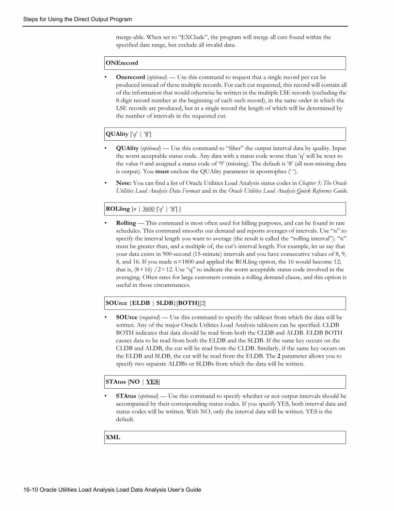
Steps for Using the Direct Output Program
merge-able. When set to “EXClude”, the program will merge all cuts found within the specified date range, but exclude all invalid data.
• Onerecord (optional) — Use this command to request that a single record per cut be produced instead of these multiple records. For each cut requested, this record will contain all of the information that would otherwise be written in the multiple LSE records (excluding the 8-digit record number at the beginning of each such record), in the same order in which the LSE records are produced, but in a single record the length of which will be determined by the number of intervals in the requested cut.
• QUAlity (optional) — Use this command to “filter” the output interval data by quality. Input the worst acceptable status code. Any data with a status code worse than ‘q’ will be reset to the value 0 and assigned a status code of ‘9’ (missing). The default is ‘8’ (all non-missing data is output). You must enclose the QUAlity parameter in apostrophes (‘ ‘).
• Note: You can find a list of Oracle Utilities Load Analysis status codes in Chapter 3: The Oracle Utilities Load Analysis Data Formats and in the Oracle Utilities Load Analysis Quick Reference Guide.
• Rolling — This command is most often used for billing purposes, and can be found in rate schedules. This command smooths out demand and reports averages of intervals. Use “n” to specify the interval length you want to average (the result is called the “rolling interval”). “n” must be greater than, and a multiple of, the cut’s interval length. For example, let us say that your data exists in 900-second (15-minute) intervals and you have consecutive values of 8, 9, 8, and 16. If you made n=1800 and applied the ROLling option, the 16 would become 12; that is, (8+16) /2=12. Use “q” to indicate the worst acceptable status code involved in the averaging. Often rates for large customers contain a rolling demand clause, and this option is useful in those circumstances.
• SOUrce (required) — Use this command to specify the tableset from which the data will be written. Any of the major Oracle Utilities Load Analysis tablesets can be specified. CLDB BOTH indicates that data should be read from both the CLDB and ALDB. ELDB BOTH causes data to be read from both the ELDB and the SLDB. If the same key occurs on the CLDB and ALDB, the cut will be read from the CLDB. Similarly, if the same key occurs on the ELDB and SLDB, the cut will be read from the ELDB. The 2 parameter allows you to specify two separate ALDBs or SLDBs from which the data will be written.
.• STAtus (optional) — Use this command to specify whether or not output intervals should be accompanied by their corresponding status codes. If you specify YES, both interval data and status codes will be written. With NO, only the interval data will be written. YES is the default.
ONErecord
QUAlity [‘q’ | ‘8’]
ROLling [n | 3600 [‘q’ | ‘8’] ]
SOUrce {ELDB | SLDB}[BOTH][2]
STAtus [NO | YES]
XML
16-10 Oracle Utilities Load Analysis Load Data Analysis User’s Guide
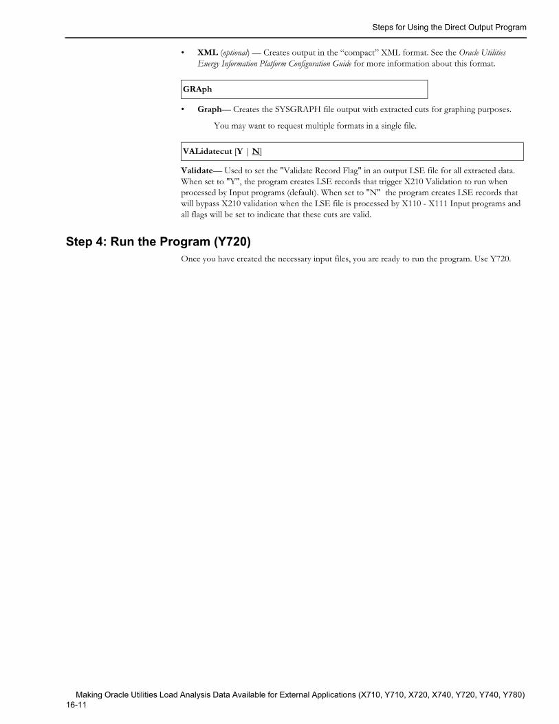
Steps for Using the Direct Output Program
• XML (optional) — Creates output in the “compact” XML format. See the Oracle Utilities Energy Information Platform Configuration Guide for more information about this format.
• Graph— Creates the SYSGRAPH file output with extracted cuts for graphing purposes.
You may want to request multiple formats in a single file.
Validate— Used to set the "Validate Record Flag" in an output LSE file for all extracted data. When set to "Y", the program creates LSE records that trigger X210 Validation to run when processed by Input programs (default). When set to "N" the program creates LSE records that will bypass X210 validation when the LSE file is processed by X110 - X111 Input programs and all flags will be set to indicate that these cuts are valid.
Step 4: Run the Program (Y720)Once you have created the necessary input files, you are ready to run the program. Use Y720.
GRAph
VALidatecut [Y | N]
Making Oracle Utilities Load Analysis Data Available for External Applications (X710, Y710, X720, X740, Y720, Y740, Y780) 16-11
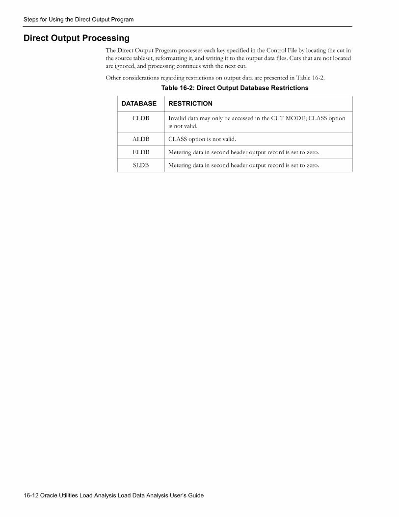
Steps for Using the Direct Output Program
Direct Output ProcessingThe Direct Output Program processes each key specified in the Control File by locating the cut in the source tableset, reformatting it, and writing it to the output data files. Cuts that are not located are ignored, and processing continues with the next cut.
Other considerations regarding restrictions on output data are presented in Table 16-2.
Table 16-2: Direct Output Database Restrictions
DATABASE RESTRICTION
CLDB Invalid data may only be accessed in the CUT MODE; CLASS option is not valid.
ALDB CLASS option is not valid.
ELDB Metering data in second header output record is set to zero.
SLDB Metering data in second header output record is set to zero.
16-12 Oracle Utilities Load Analysis Load Data Analysis User’s Guide
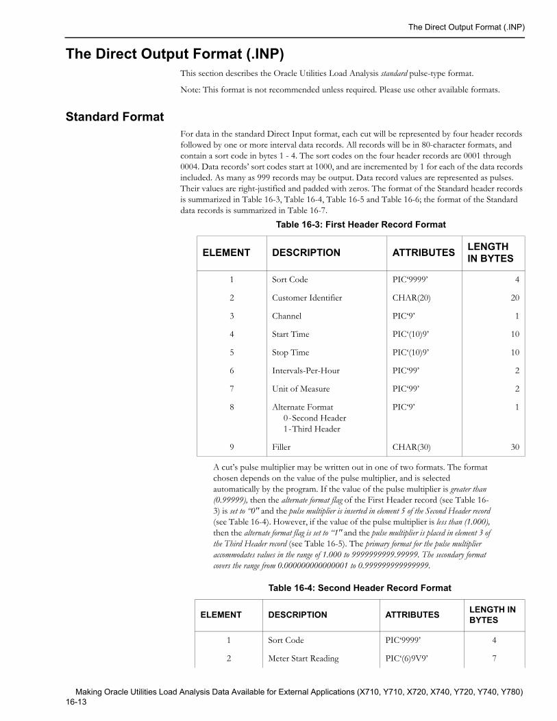
The Direct Output Format (.INP)
The Direct Output Format (.INP)This section describes the Oracle Utilities Load Analysis standard pulse-type format.
Note: This format is not recommended unless required. Please use other available formats.
Standard FormatFor data in the standard Direct Input format, each cut will be represented by four header records followed by one or more interval data records. All records will be in 80-character formats, and contain a sort code in bytes 1 - 4. The sort codes on the four header records are 0001 through 0004. Data records’ sort codes start at 1000, and are incremented by 1 for each of the data records included. As many as 999 records may be output. Data record values are represented as pulses. Their values are right-justified and padded with zeros. The format of the Standard header records is summarized in Table 16-3, Table 16-4, Table 16-5 and Table 16-6; the format of the Standard data records is summarized in Table 16-7.
A cut’s pulse multiplier may be written out in one of two formats. The format chosen depends on the value of the pulse multiplier, and is selected automatically by the program. If the value of the pulse multiplier is greater than (0.99999), then the alternate format flag of the First Header record (see Table 16-3) is set to “0" and the pulse multiplier is inserted in element 5 of the Second Header record (see Table 16-4). However, if the value of the pulse multiplier is less than (1.000), then the alternate format flag is set to “1" and the pulse multiplier is placed in element 3 of the Third Header record (see Table 16-5). The primary format for the pulse multiplier accommodates values in the range of 1.000 to 9999999999.99999. The secondary format covers the range from 0.000000000000001 to 0.999999999999999.
Table 16-3: First Header Record Format
ELEMENT DESCRIPTION ATTRIBUTES LENGTH IN BYTES
1 Sort Code PIC‘9999’ 4
2 Customer Identifier CHAR(20) 20
3 Channel PIC‘9’ 1
4 Start Time PIC‘(10)9’ 10
5 Stop Time PIC‘(10)9’ 10
6 Intervals-Per-Hour PIC‘99’ 2
7 Unit of Measure PIC‘99’ 2
8 Alternate Format 0-Second Header 1-Third Header
PIC‘9’ 1
9 Filler CHAR(30) 30
Table 16-4: Second Header Record Format
ELEMENT DESCRIPTION ATTRIBUTES LENGTH IN BYTES
1 Sort Code PIC‘9999’ 4
2 Meter Start Reading PIC‘(6)9V9’ 7
Making Oracle Utilities Load Analysis Data Available for External Applications (X710, Y710, X720, X740, Y720, Y740, Y780) 16-13
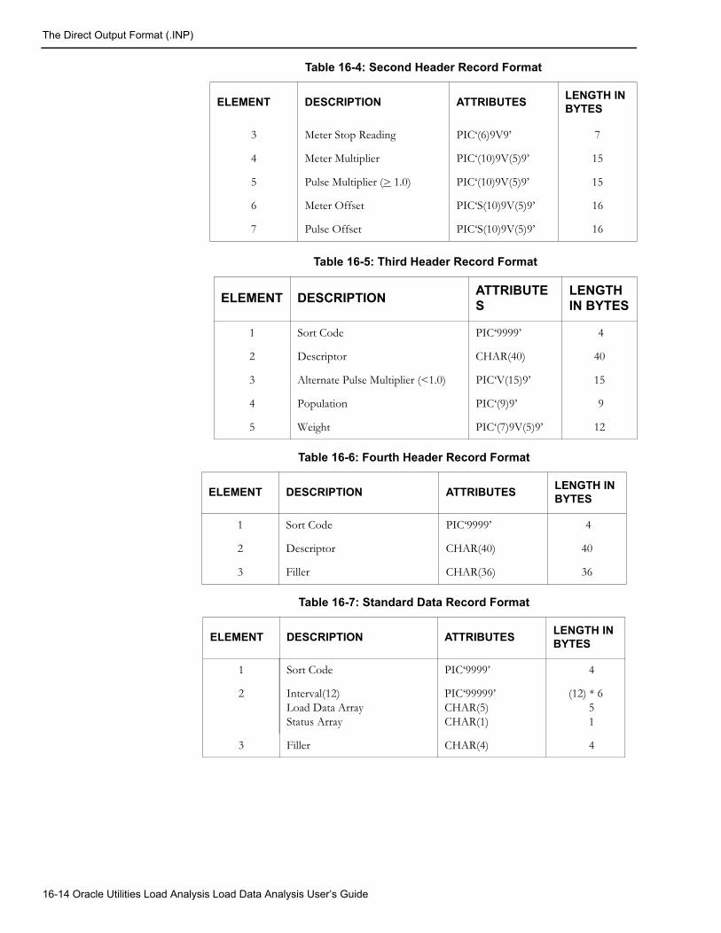
The Direct Output Format (.INP)
3 Meter Stop Reading PIC‘(6)9V9’ 7
4 Meter Multiplier PIC‘(10)9V(5)9’ 15
5 Pulse Multiplier (> 1.0) PIC‘(10)9V(5)9’ 15
6 Meter Offset PIC‘S(10)9V(5)9’ 16
7 Pulse Offset PIC‘S(10)9V(5)9’ 16
Table 16-5: Third Header Record Format
ELEMENT DESCRIPTION ATTRIBUTES
LENGTH IN BYTES
1 Sort Code PIC‘9999’ 4
2 Descriptor CHAR(40) 40
3 Alternate Pulse Multiplier (<1.0) PIC‘V(15)9’ 15
4 Population PIC‘(9)9’ 9
5 Weight PIC‘(7)9V(5)9’ 12
Table 16-6: Fourth Header Record Format
ELEMENT DESCRIPTION ATTRIBUTES LENGTH IN BYTES
1 Sort Code PIC‘9999’ 4
2 Descriptor CHAR(40) 40
3 Filler CHAR(36) 36
Table 16-7: Standard Data Record Format
ELEMENT DESCRIPTION ATTRIBUTES LENGTH IN BYTES
1 Sort Code PIC‘9999’ 4
2 Interval(12)Load Data ArrayStatus Array
PIC‘99999’CHAR(5)CHAR(1)
(12) * 6 5 1
3 Filler CHAR(4) 4
Table 16-4: Second Header Record Format
ELEMENT DESCRIPTION ATTRIBUTES LENGTH IN BYTES
16-14 Oracle Utilities Load Analysis Load Data Analysis User’s Guide
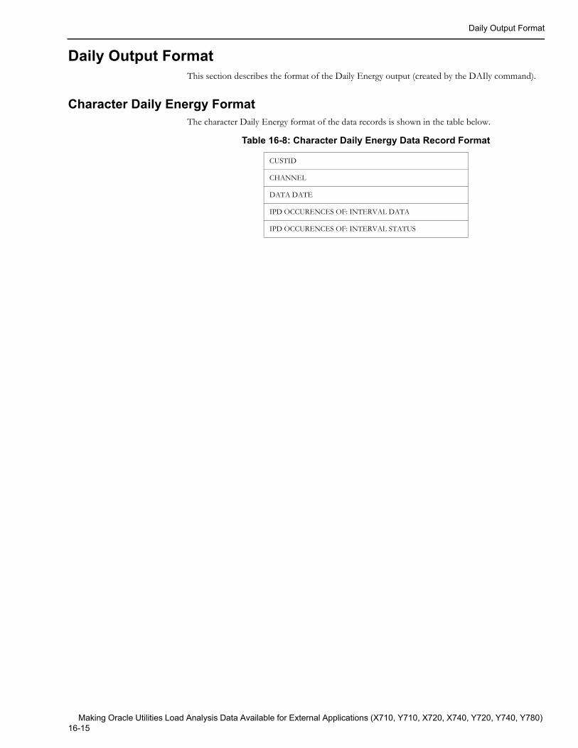
Daily Output Format
Daily Output FormatThis section describes the format of the Daily Energy output (created by the DAIly command).
Character Daily Energy FormatThe character Daily Energy format of the data records is shown in the table below.
Table 16-8: Character Daily Energy Data Record Format
CUSTID
CHANNEL
DATA DATE
IPD OCCURENCES OF: INTERVAL DATA
IPD OCCURENCES OF: INTERVAL STATUS
Making Oracle Utilities Load Analysis Data Available for External Applications (X710, Y710, X720, X740, Y720, Y740, Y780) 16-15
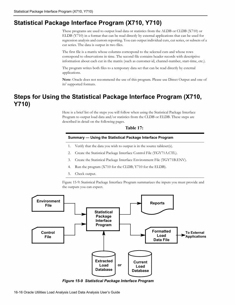
Statistical Package Interface Program (X710, Y710)
Statistical Package Interface Program (X710, Y710)These programs are used to output load data or statistics from the ALDB or CLDB (X710) or ELDB (Y710) in a format that can be read directly by external applications that can be used for regression analysis and custom reporting. You can output individual cuts, cut series, or subsets of a cut series. The data is output in two files.
The first file is a matrix whose columns correspond to the selected cuts and whose rows correspond to observations in time. The second file contains header records with descriptive information about each cut in the matrix (such as customer-id, channel-number, start-time, etc.).
The program writes both files to a temporary data set that can be read directly by external applications.
Note: Oracle does not recommend the use of this program. Please use Direct Output and one of its' supported formats.
Steps for Using the Statistical Package Interface Program (X710, Y710)
Here is a brief list of the steps you will follow when using the Statistical Package Interface Program to output load data and/or statistics from the CLDB or ELDB. These steps are described in detail on the following pages.
Figure 15-9: Statistical Package Interface Program summarizes the inputs you must provide and the outputs you can expect.
Figure 15-9 Statistical Package Interface Program
Table 17:
Summary — Using the Statistical Package Interface Program
1. Verify that the data you wish to output is in the source tableset(s).
2. Create the Statistical Package Interface Control File (TGY71A.CTL).
3. Create the Statistical Package Interface Environment File (TGY71B.ENV).
4. Run the program (X710 for the CLDB; Y710 for the ELDB).
5. Check output.
StatisticalPackageInterfaceProgram
FormattedLoad
Data File
ReportsEnvironmentFile
ControlFile
ExtractedLoad
Database
To ExternalApplications
orCurrent
LoadDatabase
16-16 Oracle Utilities Load Analysis Load Data Analysis User’s Guide
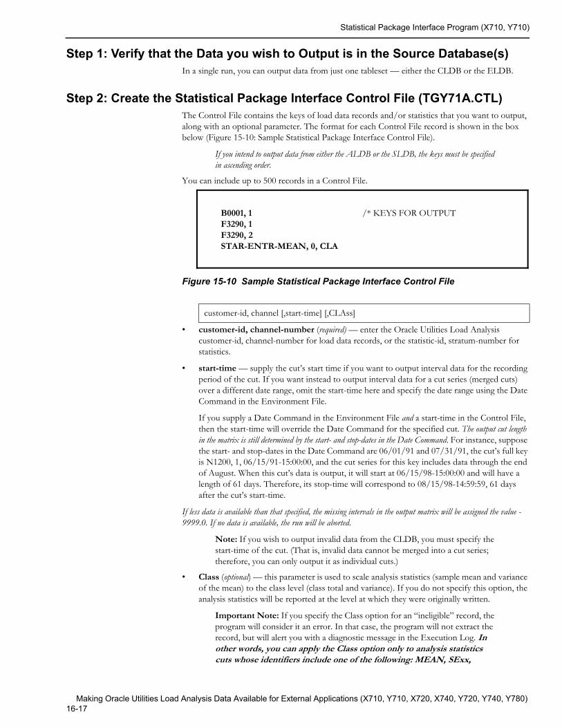
Statistical Package Interface Program (X710, Y710)
Step 1: Verify that the Data you wish to Output is in the Source Database(s)In a single run, you can output data from just one tableset — either the CLDB or the ELDB.
Step 2: Create the Statistical Package Interface Control File (TGY71A.CTL)The Control File contains the keys of load data records and/or statistics that you want to output, along with an optional parameter. The format for each Control File record is shown in the box below (Figure 15-10: Sample Statistical Package Interface Control File).
If you intend to output data from either the ALDB or the SLDB, the keys must be specified in ascending order.
You can include up to 500 records in a Control File.
Figure 15-10 Sample Statistical Package Interface Control File
• customer-id, channel-number (required) — enter the Oracle Utilities Load Analysis customer-id, channel-number for load data records, or the statistic-id, stratum-number for statistics.
• start-time — supply the cut’s start time if you want to output interval data for the recording period of the cut. If you want instead to output interval data for a cut series (merged cuts) over a different date range, omit the start-time here and specify the date range using the Date Command in the Environment File.
If you supply a Date Command in the Environment File and a start-time in the Control File, then the start-time will override the Date Command for the specified cut. The output cut length in the matrix is still determined by the start- and stop-dates in the Date Command. For instance, suppose the start- and stop-dates in the Date Command are 06/01/91 and 07/31/91, the cut’s full key is N1200, 1, 06/15/91-15:00:00, and the cut series for this key includes data through the end of August. When this cut’s data is output, it will start at 06/15/98-15:00:00 and will have a length of 61 days. Therefore, its stop-time will correspond to 08/15/98-14:59:59, 61 days after the cut’s start-time.
If less data is available than that specified, the missing intervals in the output matrix will be assigned the value -9999.0. If no data is available, the run will be aborted.
Note: If you wish to output invalid data from the CLDB, you must specify the start-time of the cut. (That is, invalid data cannot be merged into a cut series; therefore, you can only output it as individual cuts.)
• Class (optional) — this parameter is used to scale analysis statistics (sample mean and variance of the mean) to the class level (class total and variance). If you do not specify this option, the analysis statistics will be reported at the level at which they were originally written.
Important Note: If you specify the Class option for an “ineligible” record, the program will consider it an error. In that case, the program will not extract the record, but will alert you with a diagnostic message in the Execution Log. In other words, you can apply the Class option only to analysis statistics cuts whose identifiers include one of the following: MEAN, SExx,
customer-id, channel [,start-time] [,CLAss]
B0001, 1F3290, 1F3290, 2STAR-ENTR-MEAN, 0, CLA
/* KEYS FOR OUTPUT
Making Oracle Utilities Load Analysis Data Available for External Applications (X710, Y710, X720, X740, Y720, Y740, Y780) 16-17
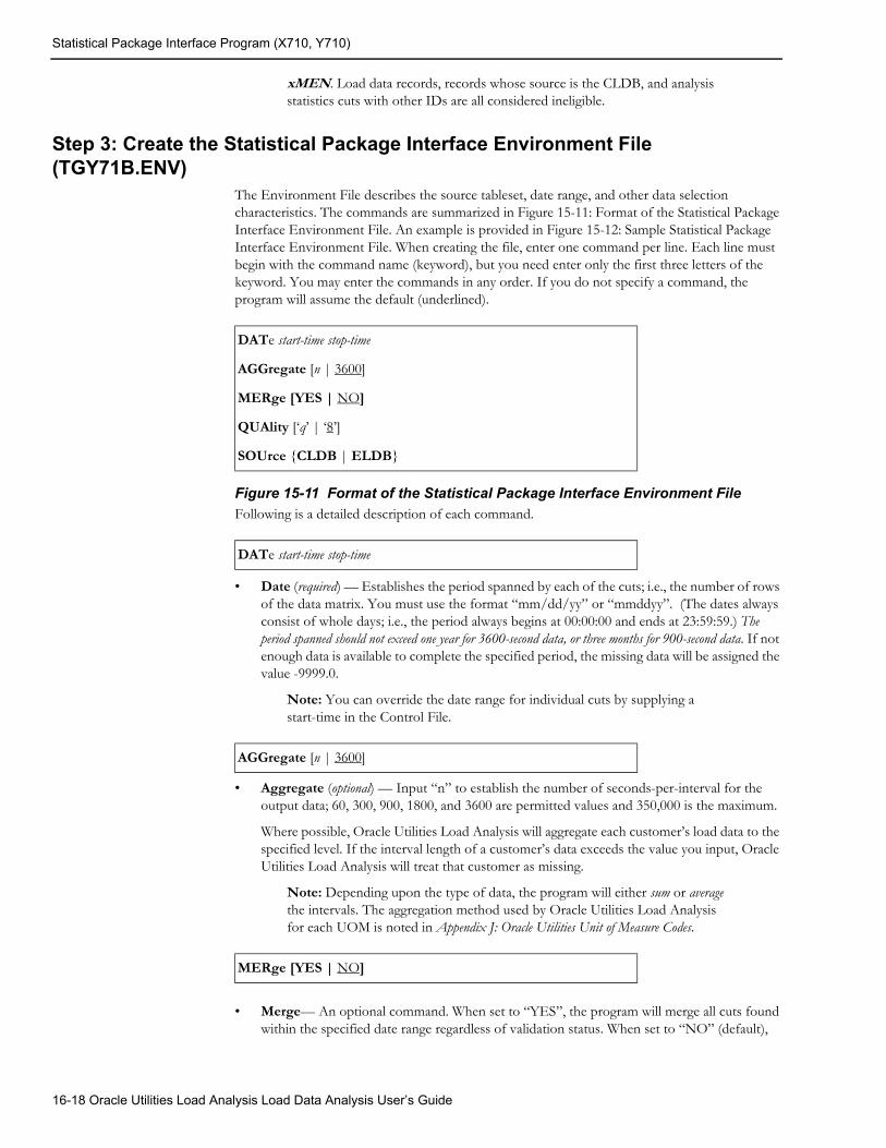
Statistical Package Interface Program (X710, Y710)
xMEN. Load data records, records whose source is the CLDB, and analysis statistics cuts with other IDs are all considered ineligible.
Step 3: Create the Statistical Package Interface Environment File (TGY71B.ENV)
The Environment File describes the source tableset, date range, and other data selection characteristics. The commands are summarized in Figure 15-11: Format of the Statistical Package Interface Environment File. An example is provided in Figure 15-12: Sample Statistical Package Interface Environment File. When creating the file, enter one command per line. Each line must begin with the command name (keyword), but you need enter only the first three letters of the keyword. You may enter the commands in any order. If you do not specify a command, the program will assume the default (underlined).
Figure 15-11 Format of the Statistical Package Interface Environment FileFollowing is a detailed description of each command.
• Date (required) — Establishes the period spanned by each of the cuts; i.e., the number of rows of the data matrix. You must use the format “mm/dd/yy” or “mmddyy”. (The dates always consist of whole days; i.e., the period always begins at 00:00:00 and ends at 23:59:59.) The period spanned should not exceed one year for 3600-second data, or three months for 900-second data. If not enough data is available to complete the specified period, the missing data will be assigned the value -9999.0.
Note: You can override the date range for individual cuts by supplying a start-time in the Control File.
• Aggregate (optional) — Input “n” to establish the number of seconds-per-interval for the output data; 60, 300, 900, 1800, and 3600 are permitted values and 350,000 is the maximum.
Where possible, Oracle Utilities Load Analysis will aggregate each customer’s load data to the specified level. If the interval length of a customer’s data exceeds the value you input, Oracle Utilities Load Analysis will treat that customer as missing.
Note: Depending upon the type of data, the program will either sum or average the intervals. The aggregation method used by Oracle Utilities Load Analysis for each UOM is noted in Appendix J: Oracle Utilities Unit of Measure Codes.
• Merge— An optional command. When set to “YES”, the program will merge all cuts found within the specified date range regardless of validation status. When set to “NO” (default),
DATe start-time stop-time
AGGregate [n | 3600]
MERge [YES | NO]
QUAlity [‘q’ | ‘8’]
SOUrce {CLDB | ELDB}
DATe start-time stop-time
AGGregate [n | 3600]
MERge [YES | NO]
16-18 Oracle Utilities Load Analysis Load Data Analysis User’s Guide
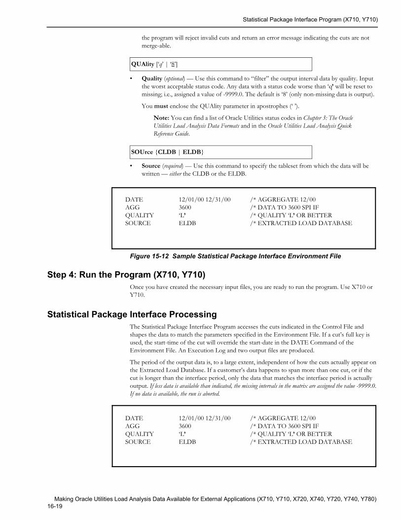
Statistical Package Interface Program (X710, Y710)
the program will reject invalid cuts and return an error message indicating the cuts are not merge-able.
• Quality (optional) — Use this command to “filter” the output interval data by quality. Input the worst acceptable status code. Any data with a status code worse than ‘q’ will be reset to missing; i.e., assigned a value of -9999.0. The default is ‘8’ (only non-missing data is output).
You must enclose the QUAlity parameter in apostrophes (‘ ’).
Note: You can find a list of Oracle Utilities status codes in Chapter 3: The Oracle Utilities Load Analysis Data Formats and in the Oracle Utilities Load Analysis Quick Reference Guide.
• Source (required) — Use this command to specify the tableset from which the data will be written — either the CLDB or the ELDB.
Figure 15-12 Sample Statistical Package Interface Environment File
Step 4: Run the Program (X710, Y710)Once you have created the necessary input files, you are ready to run the program. Use X710 or Y710.
Statistical Package Interface ProcessingThe Statistical Package Interface Program accesses the cuts indicated in the Control File and shapes the data to match the parameters specified in the Environment File. If a cut’s full key is used, the start-time of the cut will override the start-date in the DATE Command of the Environment File. An Execution Log and two output files are produced.
The period of the output data is, to a large extent, independent of how the cuts actually appear on the Extracted Load Database. If a customer’s data happens to span more than one cut, or if the cut is longer than the interface period, only the data that matches the interface period is actually output. If less data is available than indicated, the missing intervals in the matrix are assigned the value -9999.0. If no data is available, the run is aborted.
QUAlity [‘q’ | ‘8’]
SOUrce {CLDB | ELDB}
DATEAGGQUALITYSOURCE
/* AGGREGATE 12/00/* DATA TO 3600 SPI IF/* QUALITY ‘L’ OR BETTER/* EXTRACTED LOAD DATABASE
12/01/00 12/31/00 3600‘L’ELDB
DATEAGGQUALITYSOURCE
/* AGGREGATE 12/00/* DATA TO 3600 SPI IF/* QUALITY ‘L’ OR BETTER/* EXTRACTED LOAD DATABASE
12/01/00 12/31/00 3600‘L’ELDB
Making Oracle Utilities Load Analysis Data Available for External Applications (X710, Y710, X720, X740, Y720, Y740, Y780) 16-19
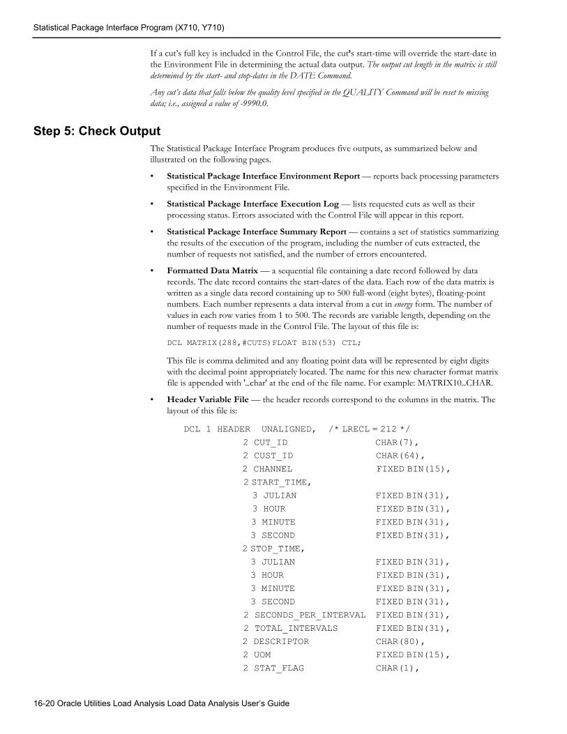
Statistical Package Interface Program (X710, Y710)
If a cut’s full key is included in the Control File, the cut’s start-time will override the start-date in the Environment File in determining the actual data output. The output cut length in the matrix is still determined by the start- and stop-dates in the DATE Command.
Any cut’s data that falls below the quality level specified in the QUALITY Command will be reset to missing data; i.e., assigned a value of -9990.0.
Step 5: Check OutputThe Statistical Package Interface Program produces five outputs, as summarized below and illustrated on the following pages.
• Statistical Package Interface Environment Report — reports back processing parameters specified in the Environment File.
• Statistical Package Interface Execution Log — lists requested cuts as well as their processing status. Errors associated with the Control File will appear in this report.
• Statistical Package Interface Summary Report — contains a set of statistics summarizing the results of the execution of the program, including the number of cuts extracted, the number of requests not satisfied, and the number of errors encountered.
• Formatted Data Matrix — a sequential file containing a date record followed by data records. The date record contains the start-dates of the data. Each row of the data matrix is written as a single data record containing up to 500 full-word (eight bytes), floating-point numbers. Each number represents a data interval from a cut in energy form. The number of values in each row varies from 1 to 500. The records are variable length, depending on the number of requests made in the Control File. The layout of this file is:
DCL MATRIX(288,#CUTS)FLOAT BIN(53) CTL;
This file is comma delimited and any floating point data will be represented by eight digits with the decimal point appropriately located. The name for this new character format matrix file is appended with '_char' at the end of the file name. For example: MATRIX10_CHAR.
• Header Variable File — the header records correspond to the columns in the matrix. The layout of this file is:
DCL 1 HEADER UNALIGNED, /* LRECL = 212 */ 2 CUT_ID CHAR(7), 2 CUST_ID CHAR(64), 2 CHANNEL FIXED BIN(15), 2 START_TIME,
3 JULIAN FIXED BIN(31), 3 HOUR FIXED BIN(31), 3 MINUTE FIXED BIN(31), 3 SECOND FIXED BIN(31), 2 STOP_TIME, 3 JULIAN FIXED BIN(31), 3 HOUR FIXED BIN(31), 3 MINUTE FIXED BIN(31), 3 SECOND FIXED BIN(31),
2 SECONDS_PER_INTERVAL FIXED BIN(31), 2 TOTAL_INTERVALS FIXED BIN(31), 2 DESCRIPTOR CHAR(80), 2 UOM FIXED BIN(15), 2 STAT_FLAG CHAR(1),
16-20 Oracle Utilities Load Analysis Load Data Analysis User’s Guide
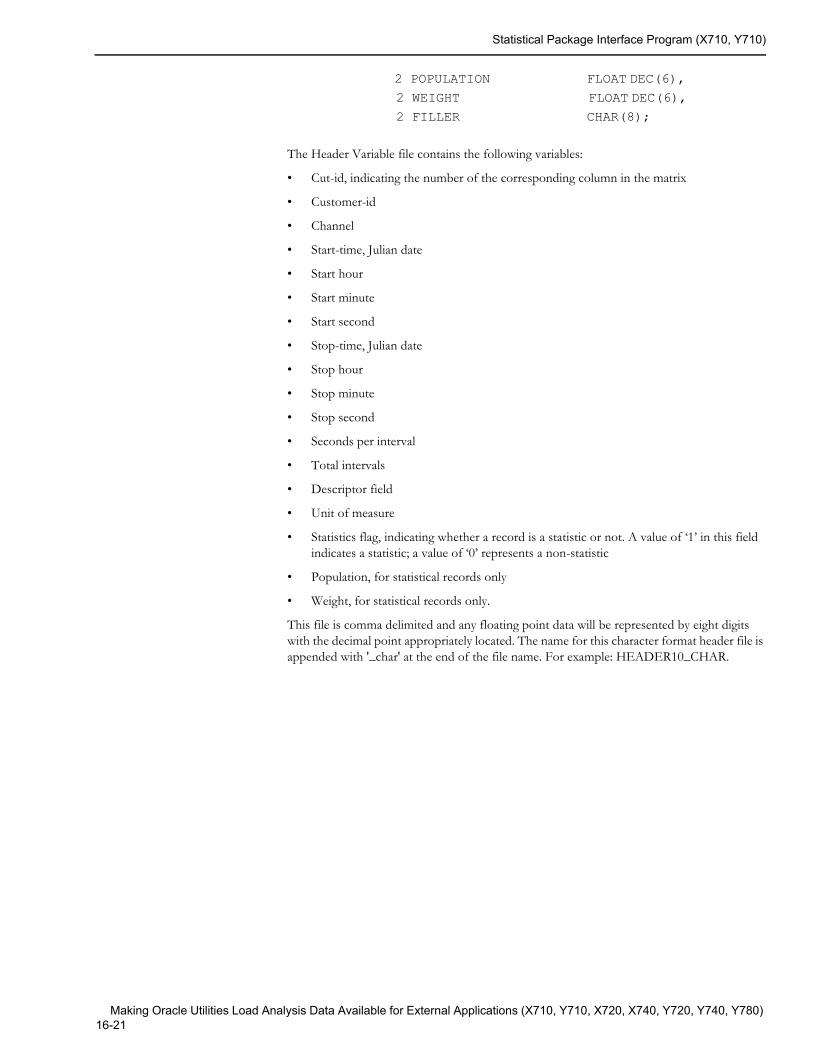
Statistical Package Interface Program (X710, Y710)
2 POPULATION FLOAT DEC(6), 2 WEIGHT FLOAT DEC(6), 2 FILLER CHAR(8);
The Header Variable file contains the following variables:
• Cut-id, indicating the number of the corresponding column in the matrix
• Customer-id
• Channel
• Start-time, Julian date
• Start hour
• Start minute
• Start second
• Stop-time, Julian date
• Stop hour
• Stop minute
• Stop second
• Seconds per interval
• Total intervals
• Descriptor field
• Unit of measure
• Statistics flag, indicating whether a record is a statistic or not. A value of ‘1’ in this field indicates a statistic; a value of ‘0’ represents a non-statistic
• Population, for statistical records only
• Weight, for statistical records only.
This file is comma delimited and any floating point data will be represented by eight digits with the decimal point appropriately located. The name for this character format header file is appended with '_char' at the end of the file name. For example: HEADER10_CHAR.
Making Oracle Utilities Load Analysis Data Available for External Applications (X710, Y710, X720, X740, Y720, Y740, Y780) 16-21
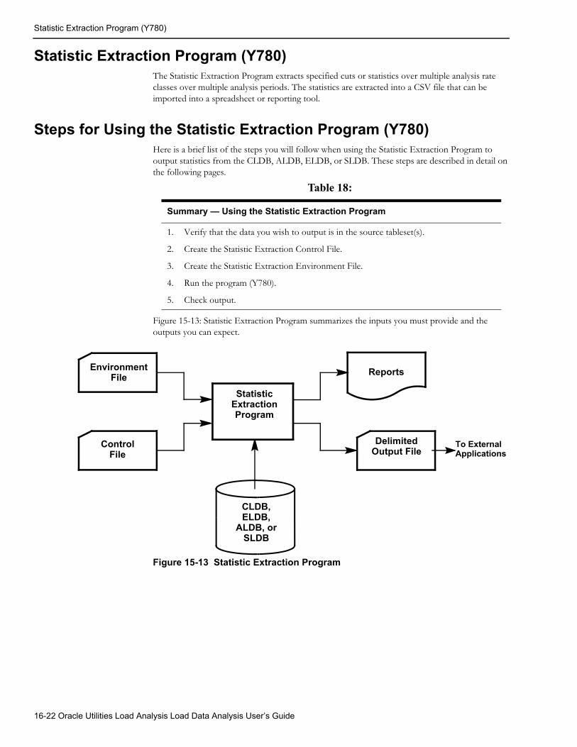
Statistic Extraction Program (Y780)
Statistic Extraction Program (Y780)The Statistic Extraction Program extracts specified cuts or statistics over multiple analysis rate classes over multiple analysis periods. The statistics are extracted into a CSV file that can be imported into a spreadsheet or reporting tool.
Steps for Using the Statistic Extraction Program (Y780)Here is a brief list of the steps you will follow when using the Statistic Extraction Program to output statistics from the CLDB, ALDB, ELDB, or SLDB. These steps are described in detail on the following pages.
Figure 15-13: Statistic Extraction Program summarizes the inputs you must provide and the outputs you can expect.
Figure 15-13 Statistic Extraction Program
Table 18:
Summary — Using the Statistic Extraction Program
1. Verify that the data you wish to output is in the source tableset(s).
2. Create the Statistic Extraction Control File.
3. Create the Statistic Extraction Environment File.
4. Run the program (Y780).
5. Check output.
StatisticExtractionProgram
Delimited Output File
ReportsEnvironmentFile
ControlFile
CLDB, ELDB,
ALDB, or SLDB
To ExternalApplications
16-22 Oracle Utilities Load Analysis Load Data Analysis User’s Guide
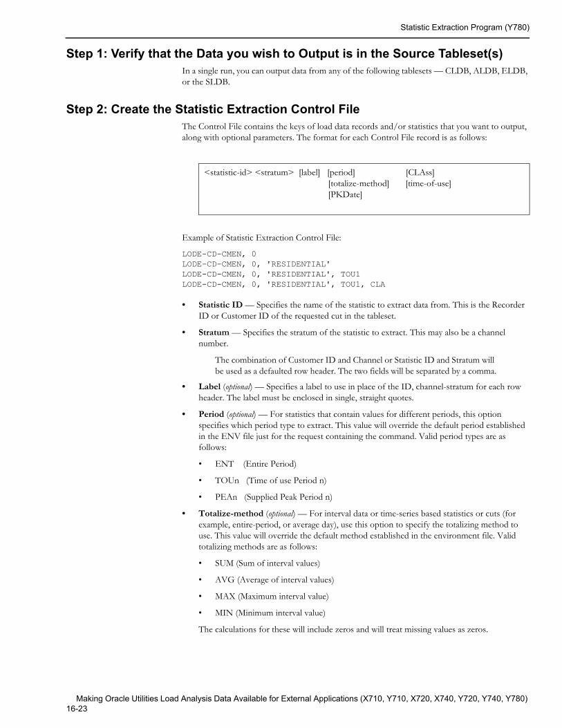
Statistic Extraction Program (Y780)
Step 1: Verify that the Data you wish to Output is in the Source Tableset(s)In a single run, you can output data from any of the following tablesets — CLDB, ALDB, ELDB, or the SLDB.
Step 2: Create the Statistic Extraction Control FileThe Control File contains the keys of load data records and/or statistics that you want to output, along with optional parameters. The format for each Control File record is as follows:
Example of Statistic Extraction Control File:
LODE-CD-CMEN, 0LODE-CD-CMEN, 0, 'RESIDENTIAL'LODE-CD-CMEN, 0, 'RESIDENTIAL', TOU1LODE-CD-CMEN, 0, 'RESIDENTIAL', TOU1, CLA
• Statistic ID — Specifies the name of the statistic to extract data from. This is the Recorder ID or Customer ID of the requested cut in the tableset.
• Stratum — Specifies the stratum of the statistic to extract. This may also be a channel number.
The combination of Customer ID and Channel or Statistic ID and Stratum will be used as a defaulted row header. The two fields will be separated by a comma.
• Label (optional) — Specifies a label to use in place of the ID, channel-stratum for each row header. The label must be enclosed in single, straight quotes.
• Period (optional) — For statistics that contain values for different periods, this option specifies which period type to extract. This value will override the default period established in the ENV file just for the request containing the command. Valid period types are as follows:
• ENT (Entire Period)
• TOUn (Time of use Period n)
• PEAn (Supplied Peak Period n)
• Totalize-method (optional) — For interval data or time-series based statistics or cuts (for example, entire-period, or average day), use this option to specify the totalizing method to use. This value will override the default method established in the environment file. Valid totalizing methods are as follows:
• SUM (Sum of interval values)
• AVG (Average of interval values)
• MAX (Maximum interval value)
• MIN (Minimum interval value)
The calculations for these will include zeros and will treat missing values as zeros.
<statistic-id> <stratum> [label] [period] [CLAss] [totalize-method] [time-of-use] [PKDate]
Making Oracle Utilities Load Analysis Data Available for External Applications (X710, Y710, X720, X740, Y720, Y740, Y780) 16-23
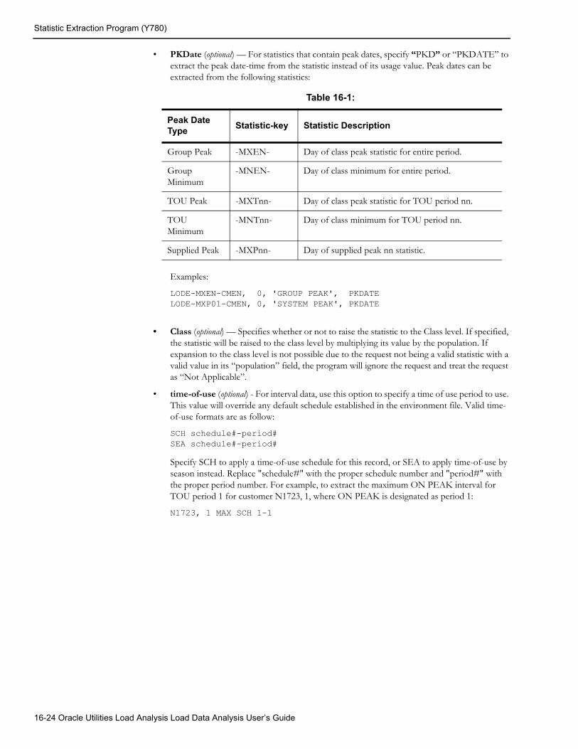
Statistic Extraction Program (Y780)
• PKDate (optional) — For statistics that contain peak dates, specify “PKD” or “PKDATE” to extract the peak date-time from the statistic instead of its usage value. Peak dates can be extracted from the following statistics:
Examples:
LODE-MXEN-CMEN, 0, 'GROUP PEAK', PKDATE LODE-MXP01-CMEN, 0, 'SYSTEM PEAK', PKDATE
• Class (optional) — Specifies whether or not to raise the statistic to the Class level. If specified, the statistic will be raised to the class level by multiplying its value by the population. If expansion to the class level is not possible due to the request not being a valid statistic with a valid value in its “population” field, the program will ignore the request and treat the request as “Not Applicable”.
• time-of-use (optional) - For interval data, use this option to specify a time of use period to use. This value will override any default schedule established in the environment file. Valid time-of-use formats are as follow:
SCH schedule#-period# SEA schedule#-period#
Specify SCH to apply a time-of-use schedule for this record, or SEA to apply time-of-use by season instead. Replace "schedule#" with the proper schedule number and "period#" with the proper period number. For example, to extract the maximum ON PEAK interval for TOU period 1 for customer N1723, 1, where ON PEAK is designated as period 1:
N1723, 1 MAX SCH 1-1
Table 16-1:
Peak Date Type Statistic-key Statistic Description
Group Peak -MXEN- Day of class peak statistic for entire period.
Group Minimum
-MNEN- Day of class minimum for entire period.
TOU Peak -MXTnn- Day of class peak statistic for TOU period nn.
TOU Minimum
-MNTnn- Day of class minimum for TOU period nn.
Supplied Peak -MXPnn- Day of supplied peak nn statistic.
16-24 Oracle Utilities Load Analysis Load Data Analysis User’s Guide
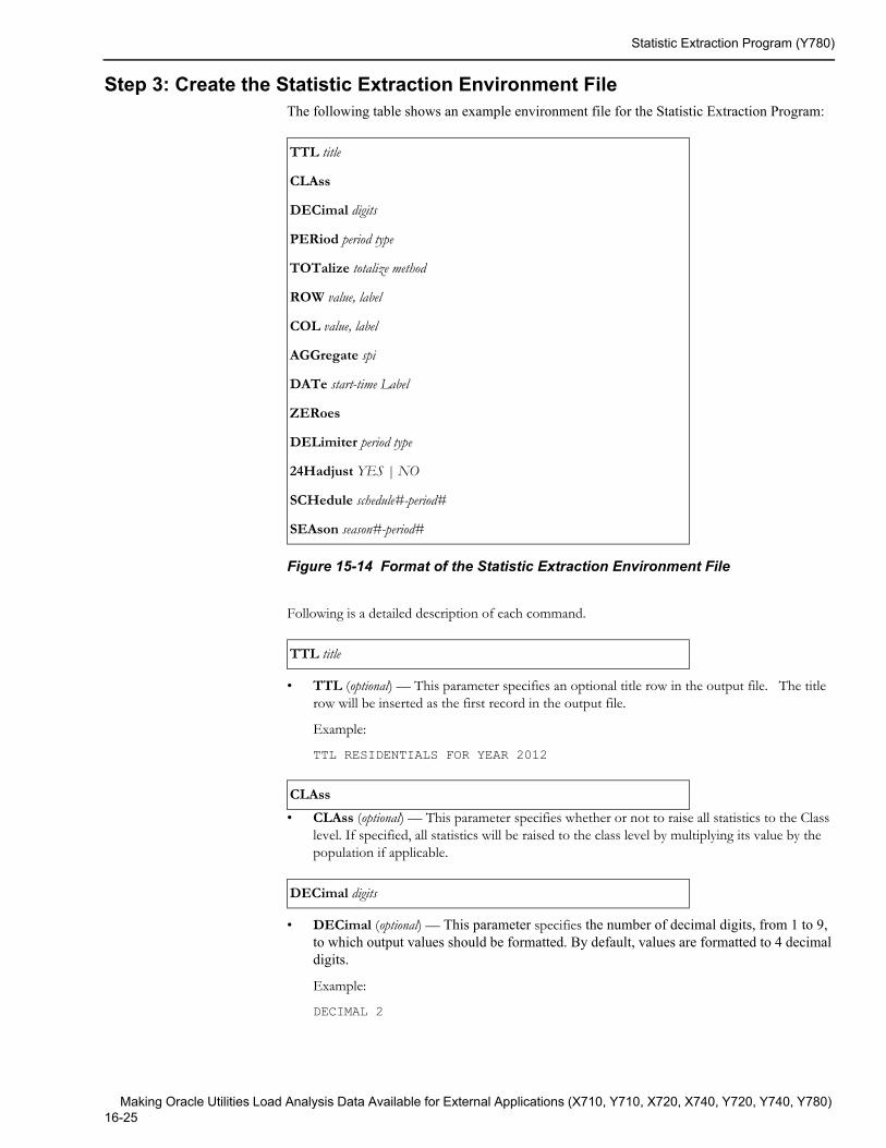
Statistic Extraction Program (Y780)
Step 3: Create the Statistic Extraction Environment FileThe following table shows an example environment file for the Statistic Extraction Program:
Figure 15-14 Format of the Statistic Extraction Environment File
Following is a detailed description of each command.
• TTL (optional) — This parameter specifies an optional title row in the output file. The title row will be inserted as the first record in the output file.
Example:
TTL RESIDENTIALS FOR YEAR 2012
• CLAss (optional) — This parameter specifies whether or not to raise all statistics to the Class level. If specified, all statistics will be raised to the class level by multiplying its value by the population if applicable.
• DECimal (optional) — This parameter specifies the number of decimal digits, from 1 to 9, to which output values should be formatted. By default, values are formatted to 4 decimal digits.
Example:
DECIMAL 2
TTL title
CLAss
DECimal digits
PERiod period type
TOTalize totalize method
ROW value, label
COL value, label
AGGregate spi
DATe start-time Label
ZERoes
DELimiter period type
24Hadjust YES | NO
SCHedule schedule#-period#
SEAson season#-period#
TTL title
CLAss
DECimal digits
Making Oracle Utilities Load Analysis Data Available for External Applications (X710, Y710, X720, X740, Y720, Y740, Y780) 16-25
Statistic Extraction Program (Y780)
• PERiod (optional) — For statistics that contain values for different time of use periods, use this option to specify the default period type to extract. Default is ENT (Entire Period). Valid period types are as follows:
• ENT (Entire Period)
• TOUn (Time of use Period n)
• PEAn (Supplied Peak Period n)
Example:
PERIOD ENTPERIOD TOU1
• TOTalize (optional) — For interval data or time-series based statistics (for example, entire-period or average day), this option specifies the mathematical method used for combining intervals. Valid types are as follows:
• SUM (Sum of interval values - Defaulted value)
• AVG (Average of interval values)
• MAX (Maximum interval value)
• MIN (Minimum interval value)
Example:
TOTALIZE SUMTOTALIZE MAX
• ROW (optional) — This parameter is used to insert an additional summary value at the end of each row containing row totals or averages. This command can be repeated to produce summary values for all value types.
“Value” specifies the value type for this row. Valid value types are TOTal and AVErage.
“Label” specifies a header label to use for this row. Default is “TOTAL” or “AVERAGE”, depending on value type. If specified, label must be enclosed in single, straight quotes.
Example:
ROW TOT 'GRAND TOTAL'
• COL (optional) — This parameter is used to insert an additional summary value at the end of each column containing column totals or averages. This command can be repeated to produce summary values for all value types. Valid value types are TOTal and AVErage
PERiod period type
TOTalize totalize method
ROW value, label
COL value, label
16-26 Oracle Utilities Load Analysis Load Data Analysis User’s Guide
Statistic Extraction Program (Y780)
“Label” (optional) specifies a header label to use for this column. Default is “TOTAL” or “AVERAGE”, depending on value type. If specified, label must be enclosed in single straight quotes.
Example:
COL TOT 'GRAND TOTAL'
• AGGregate (optional) — This parameter establishes the number of seconds-per-interval to scale the output data to. Aggregation is only applied to interval data and time-series based data. Statistic records that do not represent interval data will be ignored. Valid values are 60, 300, 900, 1800, 3600, and 86400.
Example:
AGG 3600
• DATe — Each DAT command creates a column entry in the output file. At least one DAT command entry is required. The maximum number of DAT commands allowed is 200.
Specify the start-time (analysis start periods) from which to extract statistics. The start-time, combined with statistics-id and stratum from the control file, determines which statistic record to retrieve and extract.
“Label” (optional) specifies a column header. If this header is not supplied the start-time value will be used. If specified, label must be enclosed in single straight quotes.
Example:
DAT 01/01/12-00:00:00 'JAN'
• ZERoes — By default, any data that is not extracted or not found will have a blank value as an output. The ZERoes parameter specifies that a zero value (0.0) is extracted in place of a blank value.
• DELimiter (optional) — This parameter specifies the field delimiter character to be used in the output format file. The default delimiter is comma (“,”).
• 24Hadjust (optional) — Specify YES to adjust data to 24 hour days. This setting applies only to interval data cuts. The default is NO.
AGGregate spi
DATe start-time Label
ZERoes
DELimiter value
24Hadjust YES | NO
SCHedule schedule#-period#
Making Oracle Utilities Load Analysis Data Available for External Applications (X710, Y710, X720, X740, Y720, Y740, Y780) 16-27
Statistic Extraction Program (Y780)
• SCHedule (optional) - Specify a time-of-use schedule and period to apply to all interval data records. Replace "schedule#" with the TOU schedule you wish to use and "period#" with the period number to use. For example, to apply TOU Schedule 1, ON PEAK period to all customers where ON PEAK is designated as period 1:
SCH 1-1
• SEAson (optional) - Specify to apply a time-of-use schedule based on season rather than a single time-of-use schedule. This command, if specified, supersedes the SCHedule environment command. Replace "season#" with the season number you wish to use and "period#" with the period to use. For example, to apply Season Schedule 1, ON PEAK to all customers where ON PEAK is designated as period 1:
SEA 1-1
Sample Statistic Environment File/* PROGRAM CREATES A CSV FILE/*/* RAISE TO CLA LEVEL DO NOT BLOW UP IF CANNOT RAISE TO CLASS LEVELCLA AGG 3600
/* COLUMN/ROW SUMMATIONS AND/OR TOTALS - APPENDED TO LAST COLUMNS/ROWSROW AVG 'AVERAGE' /* AVERAGE ROW ADDEDROW TOT 'TOTAL' /* TOTAL ROW ADDEDCOL AVG 'AVERAGE' /* AVERAGE COLUMN ADDEDCOL TOT 'TOTAL' /* TOTAL COLUMN ADDED
/* STATISTIC TO GO AFTER - TOT AND ON ARE FOR TIME SERIES TYPE OF CUTS/* STATISTIC ENT|[TOU1|TOUN]|[PEA1|PEAN]PER TOU1
/* CREATE THESE COLUMNS: (MAX 200)DAT 01/01/12-00:00:00 'JAN'DAT 02/01/12-00:00:00 'FEB'DAT 03/01/12-00:00:00 'MAR'DAT 04/01/12-00:00:00 'APR'DAT 05/01/12-00:00:00 'MAY'DAT 06/01/12-00:00:00 'JUN'DAT 07/01/12-00:00:00 'JUL'DAT 08/01/12-00:00:00 'AUG'DAT 09/01/12-00:00:00 'SEP'DAT 10/01/12-00:00:00 'OCT'DAT 11/01/12-00:00:00 'NOV'DAT 12/01/12-00:00:00 'DEC'
ZEROESDELIMITER ','
Step 4: Run the Program (Y780)Once you have created the necessary input files, you are ready to run the program. Use Y780.
SEAson season#-period#
16-28 Oracle Utilities Load Analysis Load Data Analysis User’s Guide
Statistic Extraction Program (Y780)
Statistic Extraction ProcessingThe program will read the environment file to establish run parameters. Any errors will halt the run and will be reported to the user in the Report.html file with a non-zero return code. The program will then read each line of the control file, overriding any environment file commands supplied for that request, read the specified tableset for the statistic or cut, then extract the data into the output file. If successful the program will return a zero return code.
Step 5: Check OutputThe Statistical Package Interface Program produces a report detailing the run execution, and a delimited file which may then be used for reporting purposes.
Making Oracle Utilities Load Analysis Data Available for External Applications (X710, Y710, X720, X740, Y720, Y740, Y780) 16-29

Statistic Extraction Program (Y780)
16-30 Oracle Utilities Load Analysis Load Data Analysis User’s Guide
Chapter 17Housekeeping (Y910 and Y960)
Oracle Utilities Load Analysis includes a number of database maintenance programs that may be performed as production processes by your System Administrator. This chapter includes a quick summary of these programs.
This chapter explains a few of the many programs Oracle Utilities Load Analysis provides for database maintenance. With these programs, you can make copies of the ELDB to protect your work, as well as move cuts from the ELDB to the SLDB and back. Programs described in this chapter include:
• Steps for Using the Archive/Delete Program (Y910)
• Steps for Using the SLDB Retrieval Program (Y960)
Housekeeping (Y910 and Y960) 17-1
Oracle Utilities Load Analysis includes various database maintenance programs that enable you to remove records from the ELDB, archive them to the “Statistics Load Database” (“SLDB”), and copy them back to the ELDB. Here is a summary of a few of the Oracle Utilities Load Analysis “housekeeping” or database maintenance programs.
This chapter emphasizes the procedures you will probably use most often:Archive/Delete and Retrieval.
It is a very good idea to establish a routine for archiving data from the ELDB to the SLDB, both in terms of when the procedure is performed and what kinds of data are preserved. Some utilities archive all statistics, but save only the load data that has been changed. It is also common for utilities to archive all monthly or yearly statistics, while others save only statistics that have been used in a rate case.
Note: It is also important that you or your I.T. staff periodically perform backup on the Database (frequency will depend on the volume of work). This helps minimize the amount of work lost in case of a hardware or software malfunction.
Name Application
Archive/Delete (Y910) Transfers cuts from the ELDB to the SLDB; deletes them from the ELDB
SLDB Retrieval (Y960) Copies cuts from the SLDB back to the ELDB, allowing you to re-examine and revise them if necessary
17-2 Oracle Utilities Load Analysis Load Data Analysis User’s Guide
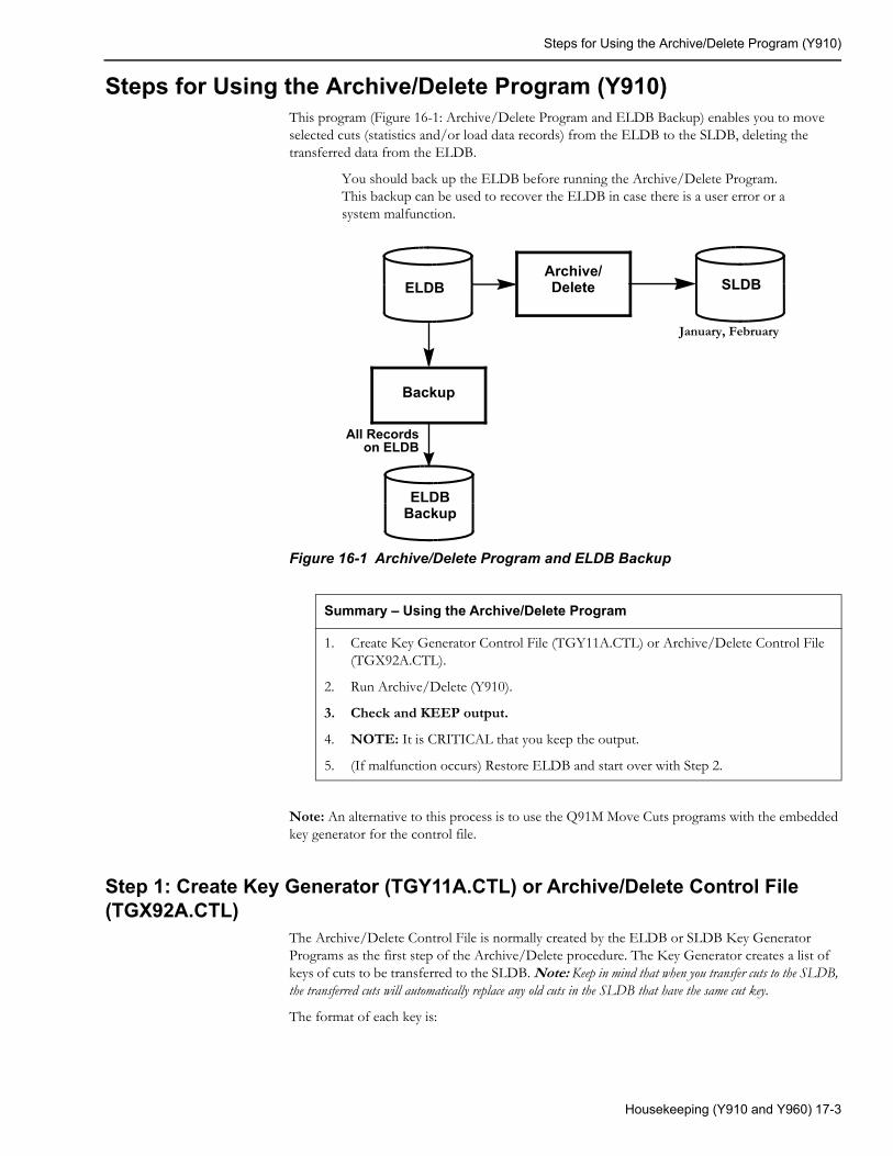
Steps for Using the Archive/Delete Program (Y910)
Steps for Using the Archive/Delete Program (Y910)This program (Figure 16-1: Archive/Delete Program and ELDB Backup) enables you to move selected cuts (statistics and/or load data records) from the ELDB to the SLDB, deleting the transferred data from the ELDB.
You should back up the ELDB before running the Archive/Delete Program. This backup can be used to recover the ELDB in case there is a user error or a system malfunction.
Figure 16-1 Archive/Delete Program and ELDB Backup
Note: An alternative to this process is to use the Q91M Move Cuts programs with the embedded key generator for the control file.
Step 1: Create Key Generator (TGY11A.CTL) or Archive/Delete Control File (TGX92A.CTL)
The Archive/Delete Control File is normally created by the ELDB or SLDB Key Generator Programs as the first step of the Archive/Delete procedure. The Key Generator creates a list of keys of cuts to be transferred to the SLDB. Note: Keep in mind that when you transfer cuts to the SLDB, the transferred cuts will automatically replace any old cuts in the SLDB that have the same cut key.
The format of each key is:
Summary – Using the Archive/Delete Program
1. Create Key Generator Control File (TGY11A.CTL) or Archive/Delete Control File (TGX92A.CTL).
2. Run Archive/Delete (Y910).
3. Check and KEEP output.
4. NOTE: It is CRITICAL that you keep the output.
5. (If malfunction occurs) Restore ELDB and start over with Step 2.
Backup
ELDBArchive/Delete SLDB
ELDBBackup
All Recordson ELDB
January, February
Housekeeping (Y910 and Y960) 17-3
Steps for Using the Archive/Delete Program (Y910)
For load data:
For statistics:
This file is created by the Key Generator, which is run prior to the archive program.
Step 2: Run Archive/Delete (Y910)Once you have created the Control File, you are ready to run the program. Use Y910.
Archive/Delete ProcessingThe Archive/Delete process usually includes two programs:
1. Key Generator
The ELDB or SLDB Key Generator is used to create a list of keys to be transferred and/or deleted. See Chapter 14: Key Generators — Shortcuts for Creating Input Files and Reports for a discussion of Key Generator processing.
2. Archive/Delete
The Archive/Delete Program is used to transfer and/or delete the above cuts.
If an archived cut already exists in the SLDB (i.e., if a cut has been returned to the ELDB via the Archive Retrieval Program and its key has not been modified), the transferred ELDB record will replace the existing one in the SLDB.
Note: To delete records off the SLDB, run the Delete Cuts Program.
Step 3: Check and KEEP OutputIt is critically important that you keep the output reports. Remember, this procedure deletes cuts from the tableset. These reports provide a record of what was deleted and when.
At the end of its run, the Archive/Delete Program produces the following reports:
• Archive/Delete Environment Report
• Archive/Delete Execution Log
• Archive/Delete Summary Log.
Step 4: ELDB Recovery (If Malfunction Occurs)If there was a malfunction during Archive/Delete, it is important that you restore the ELDB and start over. Restore the ELDB, then start over with Step 2.
customer-id, channel-number, start-time
statistic-name, strata-number, start-time
17-4 Oracle Utilities Load Analysis Load Data Analysis User’s Guide
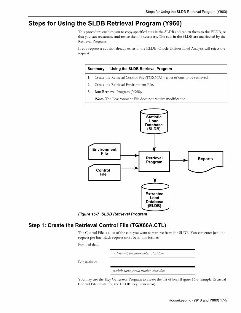
Steps for Using the SLDB Retrieval Program (Y960)
Steps for Using the SLDB Retrieval Program (Y960)This procedure enables you to copy specified cuts in the SLDB and return them to the ELDB, so that you can reexamine and revise them if necessary. The cuts in the SLDB are unaffected by the Retrieval Program.
If you request a cut that already exists in the ELDB, Oracle Utilities Load Analysis will reject the request.
Figure 16-7 SLDB Retrieval Program
Step 1: Create the Retrieval Control File (TGX66A.CTL)The Control File is a list of the cuts you want to retrieve from the SLDB. You can enter just one request per line. Each request must be in this format:
For load data:
For statistics:
You may use the Key Generator Program to create the list of keys (Figure 16-8: Sample Retrieval Control File created by the ELDB Key Generator).
Summary — Using the SLDB Retrieval Program
1. Create the Retrieval Control File (TGX66A) – a list of cuts to be retrieved.
2. Create the Retrieval Environment File.
3. Run Retrieval Program (Y960).
Note: The Environment File does not require modification.
EnvironmentFile
ExtractedLoad
Database(ELDB)
RetrievalProgram
StatisticLoad
Database(SLDB)
Reports
ControlFile
customer-id, channel-number, start-time
statistic-name, strata-number, start-time
Housekeeping (Y910 and Y960) 17-5
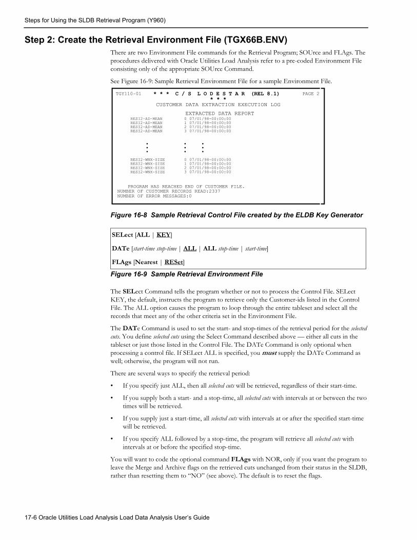
Steps for Using the SLDB Retrieval Program (Y960)
Step 2: Create the Retrieval Environment File (TGX66B.ENV)There are two Environment File commands for the Retrieval Program; SOUrce and FLAgs. The procedures delivered with Oracle Utilities Load Analysis refer to a pre-coded Environment File consisting only of the appropriate SOUrce Command.
See Figure 16-9: Sample Retrieval Environment File for a sample Environment File.
Figure 16-8 Sample Retrieval Control File created by the ELDB Key Generator
Figure 16-9 Sample Retrieval Environment File
The SELect Command tells the program whether or not to process the Control File. SELect KEY, the default, instructs the program to retrieve only the Customer-ids listed in the Control File. The ALL option causes the program to loop through the entire tableset and select all the records that meet any of the other criteria set in the Environment File.
The DATe Command is used to set the start- and stop-times of the retrieval period for the selected cuts. You define selected cuts using the Select Command described above — either all cuts in the tableset or just those listed in the Control File. The DATe Command is only optional when processing a control file. If SELect ALL is specified, you must supply the DATe Command as well; otherwise, the program will not run.
There are several ways to specify the retrieval period:
• If you specify just ALL, then all selected cuts will be retrieved, regardless of their start-time.
• If you supply both a start- and a stop-time, all selected cuts with intervals at or between the two times will be retrieved.
• If you supply just a start-time, all selected cuts with intervals at or after the specified start-time will be retrieved.
• If you specify ALL followed by a stop-time, the program will retrieve all selected cuts with intervals at or before the specified stop-time.
You will want to code the optional command FLAgs with NOR, only if you want the program to leave the Merge and Archive flags on the retrieved cuts unchanged from their status in the SLDB, rather than resetting them to “NO” (see above). The default is to reset the flags.
SELect [ALL | KEY]
DATe [start-time stop-time | ALL | ALL stop-time | start-time]
FLAgs [Nearest | RESet]
* * * C / S L O D E S T A R (REL 8.1) * * *
CUSTOMER DATA EXTRACTION EXECUTION LOGTGY110-01 PAGE 2
EXTRACTED DATA REPORT
PROGRAM HAS REACHED END OF CUSTOMER FILE.NUMBER OF CUSTOMER RECORDS READ:2337NUMBER OF ERROR MESSAGES:0
RESI2-AD-MEANRESI2-AD-MEANRESI2-AD-MEANRESI2-AD-MEAN
RESI2-WNX-SIZERESI2-WNX-SIZERESI2-WNX-SIZERESI2-WNX-SIZE
0123
0123
•••
07/01/98-00:00:0007/01/98-00:00:0007/01/98-00:00:0007/01/98-00:00:00
07/01/98-00:00:0007/01/98-00:00:0007/01/98-00:00:0007/01/98-00:00:00
•••
•••
17-6 Oracle Utilities Load Analysis Load Data Analysis User’s Guide
Steps for Using the SLDB Retrieval Program (Y960)
Step 3: Run the SLDB Retrieval ProgramSubmit the Y960 program.
Retrieval ProcessingIf a cut is found, the program will attempt to write the active record (inactive and edit trail records are not normally stored on the SLDB) for that cut to the ELDB. If a cut being retrieved already exists on the ELDB, the retrieval request is rejected.
Housekeeping (Y910 and Y960) 17-7

Steps for Using the SLDB Retrieval Program (Y960)
17-8 Oracle Utilities Load Analysis Load Data Analysis User’s Guide

Chapter 18The Cut Series Gap Report Program
(Y490 - Y491)
The Cut Series Gap Report lists, for each cut series (customer ID and channel), the start date and time of the series, any gaps in the data, and the stop date and time of the series. The report shows the start- and stop-times of each gap. A gap is defined both as a time period between the end of a cut and the beginning of the next cut in the series, and as a period of missing data (as defined by status codes) within a single cut. The Gap Report may be produced for all cut series in the ELDB or SLDB, or for a specified portion of the tableset. It reports on load data cuts and/or Entire Period statistics only.
The Gap Report can provide a quick check of the completeness of load data in your ELDB or CLDB before running an Analysis Program. Also, if you have been running an Analysis Program periodically (each month, for example), you can use the Gap Report for a selected Entire Period statistic as a check that all such runs over a longer period were completed successfully.
Once you identify the cuts with gaps, you may elect to run the X310 Load Data Editor on the cut series to fix the gaps. Please refer to Editing Data in the CLDB Using the Load Data Editor (X310 or X320) on page 9-1 in Oracle Utilities Load Analysis Load Data Analysis User’s Guide, and reference the EGAP Editor Command.
The Cut Series Gap Report Program (Y490 - Y491) 18-1
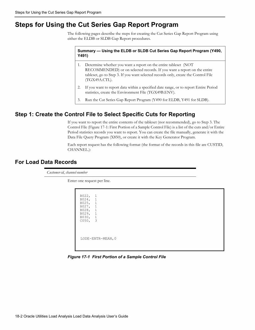
Steps for Using the Cut Series Gap Report Program
Steps for Using the Cut Series Gap Report ProgramThe following pages describe the steps for creating the Cut Series Gap Report Program using either the ELDB or SLDB Gap Report procedures.
Step 1: Create the Control File to Select Specific Cuts for ReportingIf you want to report the entire contents of the tableset (nor recommended), go to Step 3. The Control File (Figure 17-1: First Portion of a Sample Control File) is a list of the cuts and/or Entire Period statistics records you want to report. You can create the file manually, generate it with the Data File Query Program (X850), or create it with the Key Generator Program.
Each report request has the following format (the format of the records in this file are CUSTID, CHANNEL.):
For Load Data Records
Enter one request per line.
Figure 17-1 First Portion of a Sample Control File
Summary — Using the ELDB or SLDB Cut Series Gap Report Program (Y490, Y491)
1. Determine whether you want a report on the entire tableset (NOT RECOMMENDED) or on selected records. If you want a report on the entire tableset, go to Step 3. If you want selected records only, create the Control File (TGX49A.CTL).
2. If you want to report data within a specified date range, or to report Entire Period statistics, create the Environment File (TGX49B.ENV).
3. Run the Cut Series Gap Report Program (Y490 for ELDB, Y491 for SLDB).
Customer-id, channel-number
B022, 1B024, 1B025, 1B027, 1B028, 1B029, 1B030, 1C050, 3
LODE-ENTR-MEAN,0
18-2 Oracle Utilities Load Analysis Load Data Analysis User’s Guide
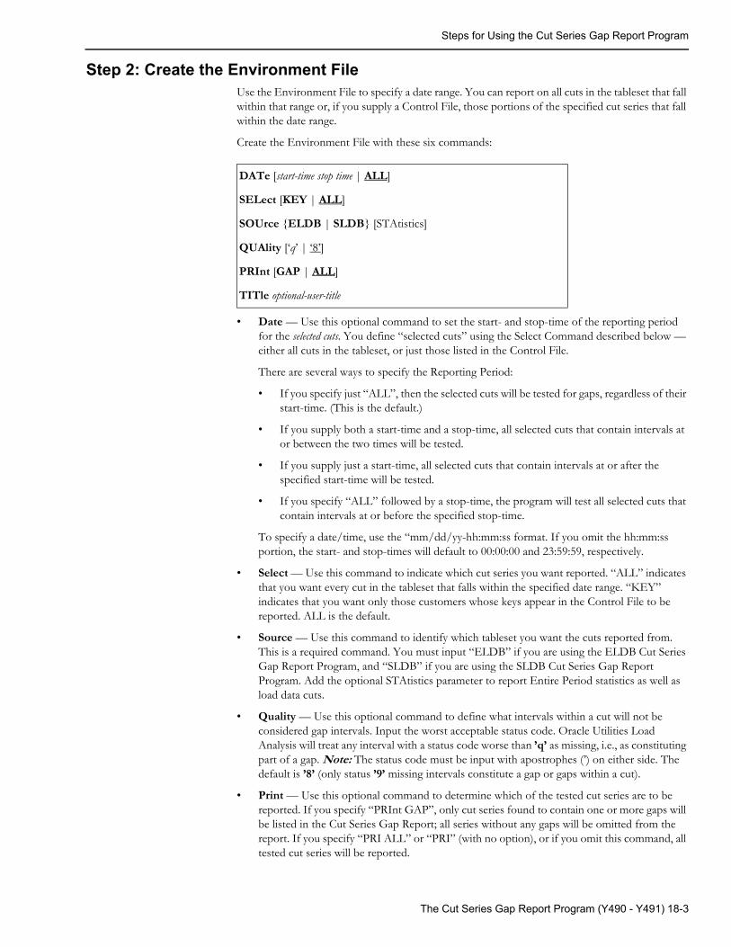
Steps for Using the Cut Series Gap Report Program
Step 2: Create the Environment FileUse the Environment File to specify a date range. You can report on all cuts in the tableset that fall within that range or, if you supply a Control File, those portions of the specified cut series that fall within the date range.
Create the Environment File with these six commands:
• Date — Use this optional command to set the start- and stop-time of the reporting period for the selected cuts. You define “selected cuts” using the Select Command described below — either all cuts in the tableset, or just those listed in the Control File.
There are several ways to specify the Reporting Period:
• If you specify just “ALL”, then the selected cuts will be tested for gaps, regardless of their start-time. (This is the default.)
• If you supply both a start-time and a stop-time, all selected cuts that contain intervals at or between the two times will be tested.
• If you supply just a start-time, all selected cuts that contain intervals at or after the specified start-time will be tested.
• If you specify “ALL” followed by a stop-time, the program will test all selected cuts that contain intervals at or before the specified stop-time.
To specify a date/time, use the “mm/dd/yy-hh:mm:ss format. If you omit the hh:mm:ss portion, the start- and stop-times will default to 00:00:00 and 23:59:59, respectively.
• Select — Use this command to indicate which cut series you want reported. “ALL” indicates that you want every cut in the tableset that falls within the specified date range. “KEY” indicates that you want only those customers whose keys appear in the Control File to be reported. ALL is the default.
• Source — Use this command to identify which tableset you want the cuts reported from. This is a required command. You must input “ELDB” if you are using the ELDB Cut Series Gap Report Program, and “SLDB” if you are using the SLDB Cut Series Gap Report Program. Add the optional STAtistics parameter to report Entire Period statistics as well as load data cuts.
• Quality — Use this optional command to define what intervals within a cut will not be considered gap intervals. Input the worst acceptable status code. Oracle Utilities Load Analysis will treat any interval with a status code worse than ’q’ as missing, i.e., as constituting part of a gap. Note: The status code must be input with apostrophes (’) on either side. The default is ’8’ (only status ’9’ missing intervals constitute a gap or gaps within a cut).
• Print — Use this optional command to determine which of the tested cut series are to be reported. If you specify “PRInt GAP”, only cut series found to contain one or more gaps will be listed in the Cut Series Gap Report; all series without any gaps will be omitted from the report. If you specify “PRI ALL” or “PRI” (with no option), or if you omit this command, all tested cut series will be reported.
DATe [start-time stop time | ALL]
SELect [KEY | ALL]
SOUrce {ELDB | SLDB} [STAtistics]
QUAlity [‘q’ | ‘8’]
PRInt [GAP | ALL]
TITle optional-user-title
The Cut Series Gap Report Program (Y490 - Y491) 18-3
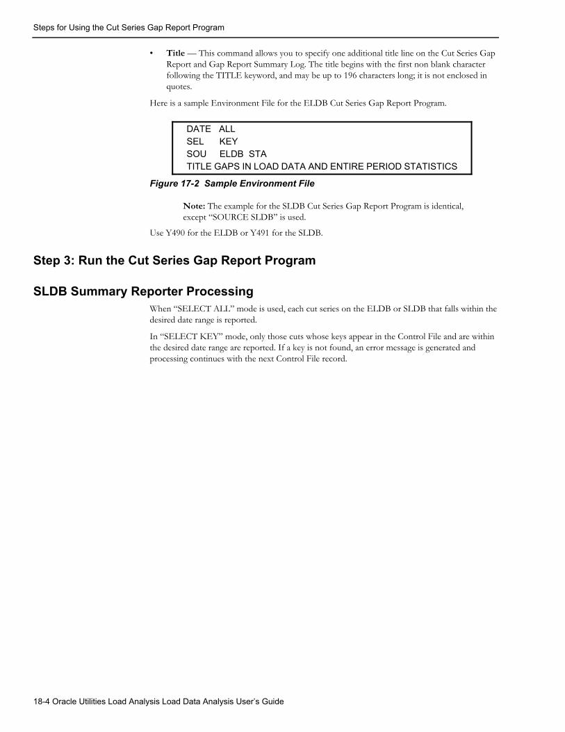
Steps for Using the Cut Series Gap Report Program
• Title — This command allows you to specify one additional title line on the Cut Series Gap Report and Gap Report Summary Log. The title begins with the first non blank character following the TITLE keyword, and may be up to 196 characters long; it is not enclosed in quotes.
Here is a sample Environment File for the ELDB Cut Series Gap Report Program.
Figure 17-2 Sample Environment File
Note: The example for the SLDB Cut Series Gap Report Program is identical, except “SOURCE SLDB” is used.
Use Y490 for the ELDB or Y491 for the SLDB.
Step 3: Run the Cut Series Gap Report Program
SLDB Summary Reporter ProcessingWhen “SELECT ALL” mode is used, each cut series on the ELDB or SLDB that falls within the desired date range is reported.
In “SELECT KEY” mode, only those cuts whose keys appear in the Control File and are within the desired date range are reported. If a key is not found, an error message is generated and processing continues with the next Control File record.
DATE ALLSEL KEYSOU ELDB STATITLE GAPS IN LOAD DATA AND ENTIRE PERIOD STATISTICS
18-4 Oracle Utilities Load Analysis Load Data Analysis User’s Guide
Chapter 19The Daytype Analysis Program (Y760 — Y770)
The Daytype Analysis Program produces 24-hour average hourly load profiles for up to 48 daytypes in a year. Up to four daytypes can be requested for a period of up to 12 months: Weekday, Weekend Day, Peak Day, and Nearpeak Day. The Daytype Analysis Program produces a report and an output file in a format for compatibility with non-Oracle Utilities Load Analysis modeling programs. The file contains a 24-hour load profile for each daytype and each calendar month or season. Multiple end-uses may be analyzed in each run. The program can also analyze statistic records written to the ELDB by analysis programs.
Data used in the analysis is extracted over the date range specified in the Environment File for each end-use (customer ID and channel) specified in the Control File, and is output as a report. If a statistic record is selected and it consists of multiple records over the date range, the records are merged; if the Class option is used, data from each of the merged records is scaled by the appropriate population factor. For each end-use or statistic, the output file consists of several header records followed by one data record per hour and month for each daytype requested. Two descriptive titles may be entered via the Environment File for inclusion in the header records. An additional description specific to each cut series, for use in the output record labeled “EE”, may be entered via the Control File; if this option is not chosen, the program will use the customer ID, channel, number of calendar months or seasons analyzed, and abbreviations of the daytypes selected.
The Daytype Analysis Program (Y760 — Y770) 19-1
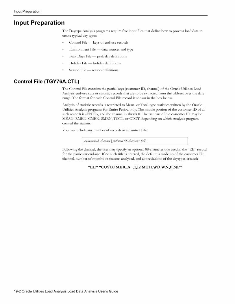
Input Preparation
Input PreparationThe Daytype Analysis programs require five input files that define how to process load data to create typical day types:
• Control File — keys of end-use records
• Environment File — data sources and type
• Peak Days File — peak day definitions
• Holiday File — holiday definitions
• Season File — season definitions.
Control File (TGY76A.CTL)The Control File contains the partial keys (customer ID, channel) of the Oracle Utilities Load Analysis end-use cuts or statistic records that are to be extracted from the tableset over the date range. The format for each Control File record is shown in the box below.
Analysis of statistic records is restricted to Mean- or Total-type statistics written by the Oracle Utilities Analysis programs for Entire Period only. The middle portion of the customer ID of all such records is -ENTR-, and the channel is always 0. The last part of the customer ID may be MEAN, RMEN, CMEN, SMEN, TOTL, or CTOT, depending on which Analysis program created the statistic.
You can include any number of records in a Control File.
Following the channel, the user may specify an optional 88-character title used in the “EE” record for the particular end-use. If no such title is entered, the default is made up of the customer ID, channel, number of months or seasons analyzed, and abbreviations of the daytypes created:
customer-id, channel [,optional 88-character title]
“EE” “CUSTOMER_A ,1,12 MTH,WD,WN,P,NP”
19-2 Oracle Utilities Load Analysis Load Data Analysis User’s Guide
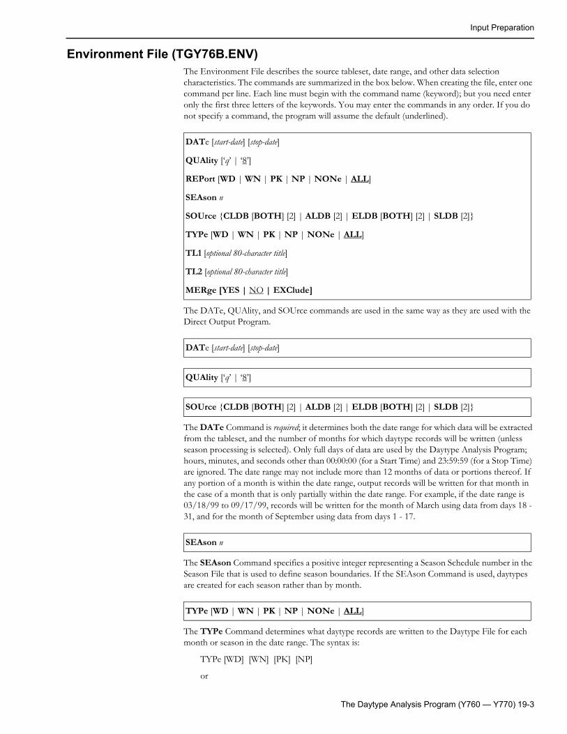
Input Preparation
Environment File (TGY76B.ENV)The Environment File describes the source tableset, date range, and other data selection characteristics. The commands are summarized in the box below. When creating the file, enter one command per line. Each line must begin with the command name (keyword); but you need enter only the first three letters of the keywords. You may enter the commands in any order. If you do not specify a command, the program will assume the default (underlined).
The DATe, QUAlity, and SOUrce commands are used in the same way as they are used with the Direct Output Program.
The DATe Command is required; it determines both the date range for which data will be extracted from the tableset, and the number of months for which daytype records will be written (unless season processing is selected). Only full days of data are used by the Daytype Analysis Program; hours, minutes, and seconds other than 00:00:00 (for a Start Time) and 23:59:59 (for a Stop Time) are ignored. The date range may not include more than 12 months of data or portions thereof. If any portion of a month is within the date range, output records will be written for that month in the case of a month that is only partially within the date range. For example, if the date range is 03/18/99 to 09/17/99, records will be written for the month of March using data from days 18 - 31, and for the month of September using data from days 1 - 17.
The SEAson Command specifies a positive integer representing a Season Schedule number in the Season File that is used to define season boundaries. If the SEAson Command is used, daytypes are created for each season rather than by month.
The TYPe Command determines what daytype records are written to the Daytype File for each month or season in the date range. The syntax is:
TYPe [WD] [WN] [PK] [NP]
or
DATe [start-date] [stop-date]
QUAlity [‘q’ | ‘8’]
REPort [WD | WN | PK | NP | NONe | ALL]
SEAson n
SOUrce {CLDB [BOTH] [2] | ALDB [2] | ELDB [BOTH] [2] | SLDB [2]}
TYPe [WD | WN | PK | NP | NONe | ALL]
TL1 [optional 80-character title]
TL2 [optional 80-character title]
MERge [YES | NO | EXClude]
DATe [start-date] [stop-date]
QUAlity [‘q’ | ‘8’]
SOUrce {CLDB [BOTH] [2] | ALDB [2] | ELDB [BOTH] [2] | SLDB [2]}
SEAson n
TYPe [WD | WN | PK | NP | NONe | ALL]
The Daytype Analysis Program (Y760 — Y770) 19-3
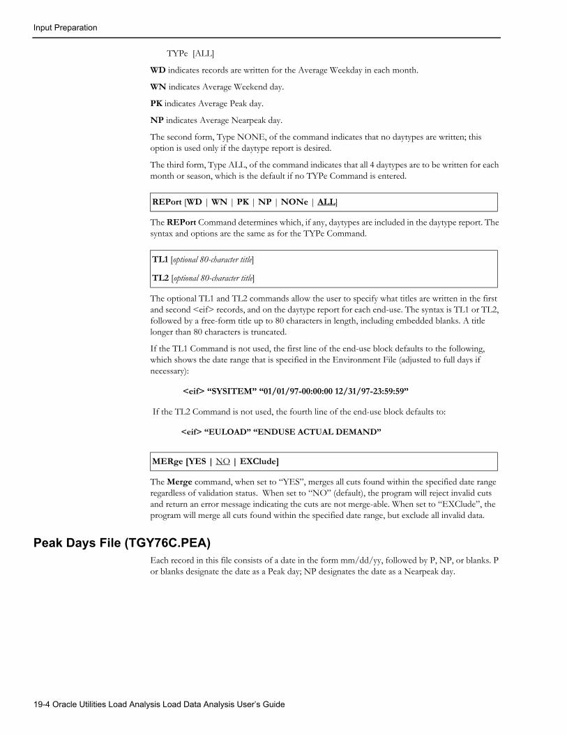
Input Preparation
TYPe [ALL]
WD indicates records are written for the Average Weekday in each month.
WN indicates Average Weekend day.
PK indicates Average Peak day.
NP indicates Average Nearpeak day.
The second form, Type NONE, of the command indicates that no daytypes are written; this option is used only if the daytype report is desired.
The third form, Type ALL, of the command indicates that all 4 daytypes are to be written for each month or season, which is the default if no TYPe Command is entered.
The REPort Command determines which, if any, daytypes are included in the daytype report. The syntax and options are the same as for the TYPe Command.
The optional TL1 and TL2 commands allow the user to specify what titles are written in the first and second <eif> records, and on the daytype report for each end-use. The syntax is TL1 or TL2, followed by a free-form title up to 80 characters in length, including embedded blanks. A title longer than 80 characters is truncated.
If the TL1 Command is not used, the first line of the end-use block defaults to the following, which shows the date range that is specified in the Environment File (adjusted to full days if necessary):
If the TL2 Command is not used, the fourth line of the end-use block defaults to:
The Merge command, when set to “YES”, merges all cuts found within the specified date range regardless of validation status. When set to “NO” (default), the program will reject invalid cuts and return an error message indicating the cuts are not merge-able. When set to “EXClude”, the program will merge all cuts found within the specified date range, but exclude all invalid data.
Peak Days File (TGY76C.PEA)Each record in this file consists of a date in the form mm/dd/yy, followed by P, NP, or blanks. P or blanks designate the date as a Peak day; NP designates the date as a Nearpeak day.
REPort [WD | WN | PK | NP | NONe | ALL]
TL1 [optional 80-character title]
TL2 [optional 80-character title]
<eif> “SYSITEM” “01/01/97-00:00:00 12/31/97-23:59:59”
<eif> “EULOAD” “ENDUSE ACTUAL DEMAND”
MERge [YES | NO | EXClude]
19-4 Oracle Utilities Load Analysis Load Data Analysis User’s Guide

Input Preparation
Holiday File (TGY31C.HOL)The program uses the standard Oracle Utilities Load Analysis Holiday File, which treats Holidays as Weekend days for this analysis. However, if a date in the Holiday File is also designated a Peak day or a Nearpeak day, the Peak/Nearpeak designation applies.
Season File (TGY31E.SEA)The program uses the standard Oracle Utilities Load Analysis Season File. Each season is defined by a season number and name and by one or more start and stop dates. Noncontiguous season segments within the Daytype Analysis date range are combined for computation of each season’s daytypes.
Processing SummaryThe Daytype Analysis Program processes each entry in the Control File over the date range specified in the Environment File. It is designed to create a set of day types for each calendar month or season spanned by that date range.
Therefore, each month or season in the date range must contain at least one example of each daytype requested by the TYPE or REPORT Command, or of all four daytypes, if no TYPE or REPORT Command is specified. Every day in the date range is classified as belonging to a daytype as follows:
• If it is in the Peak Days file, it is classified as either a Peak day or a Nearpeak day
• If it is in the Holiday File and not in the Peak Day file, it is classified as a Weekend day
• All other days are classified as either Weekdays or Weekend days according to their day of the week.
Summary of OutputsThe program creates three reports and an output file, as follows:
• Environment File Report — summary of user options and defaults
• Execution Log Report — summary of processing for each Control File entry
• Daytype Report — daytype values for each end-use or statistic, in vertical columns, one page per month or season
• Daytype File — daytype values for each end-use or statistic in DSManager file format.
The Daytype Analysis Program (Y760 — Y770) 19-5

Input Preparation
Daytype File (TGY761)The output for each end-use or statistic (customer ID, channel) begins with five header records. The first contains the title specified in the TL1 Environment File command, or the default:
The second header record is constant:
The third header record contains the title entered in the Control File record for this end-use, or the default:
The fourth header record contains the title specified in the TL1 Environment File command, or the default:
The fifth header record is constant:
Following the header records are a series of data records. Each data record contains the average demand for one hour of a particular daytype within a particular month or season. As suggested by the fifth header record, above, the data record consists of a daytype number, an hour of the day, and a demand figure.
The daytype number is assigned as follows:
• The first record for the first month or season is assigned the number 1
• All 24 hours of this daytype come next, with daytype number 1
• The next daytype for that month or season (if any) is assigned the number 2, and so forth
• The first record for the second month of season is assigned the next daytype number in sequence after the first month’s or season’s, etc.
Therefore, if all four daytypes are written, records for the first month or season are assigned daytype numbers 1 - 4, records for the second month or season are assigned daytype numbers 5 - 8, and so on.
<eif> “SYSITEM” “01/01/99-00:00:00 12/31/99-23:59:59”
“EE - ELECTRIC ENDUSE DATA”
“EE” “P1810 ,1,12 MTH,WD,WN,P,NP”
<eif> “EULOAD” “ENDUSE ACTUAL DEMAND”
“DT#” “Hour” “actual demand”
19-6 Oracle Utilities Load Analysis Load Data Analysis User’s Guide
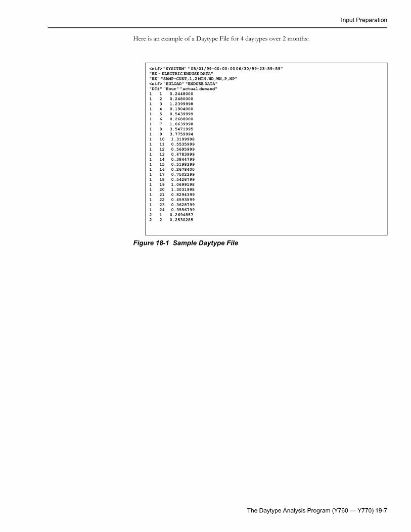
Input Preparation
Here is an example of a Daytype File for 4 daytypes over 2 months:
Figure 18-1 Sample Daytype File
<eif> "SYSITEM" " 05/01/99-00:00:00 06/30/99-23:59:59" "EE - ELECTRIC ENDUSE DATA" "EE" "SAMP-CUST,1,2 MTH,WD,WN,P,NP" <eif> "EULOAD" "ENDUSE DATA" "DT#" "Hour" "actual demand" 1 1 0.2448000 1 2 0.2480000 1 3 1.2399998 1 4 0.1904000 1 5 0.5439999 1 6 0.2688000 1 7 1.0639998 1 8 3.5471995 1 9 3.7759994 1 10 1.3199998 1 11 0.5535999 1 12 0.5695999 1 13 0.4783999 1 14 0.3844799 1 15 0.5198399 1 16 0.2678400 1 17 0.7502399 1 18 0.5428799 1 19 1.0699198 1 20 1.3031998 1 21 0.8294399 1 22 0.4593599 1 23 0.3628799 1 24 0.3556799 2 1 0.2694857 2 2 0.2530285
The Daytype Analysis Program (Y760 — Y770) 19-7

Input Preparation
19-8 Oracle Utilities Load Analysis Load Data Analysis User’s Guide
Chapter 20The Individual Customer Analysis Program
Developed in response to user requests, the Individual Customer Analysis Program (ICA) is an function of the Oracle Utilities Load Data Management and Analysis System. This program enables you to quickly generate, report, and save statistics for individual customers — including Entire Period, Time-Of-Use (TOU), and Average Day-type statistics. Because it is an efficient tool for analyzing individual customer load patterns, ICA is useful for rate comparisons, customer service, load management applications, and more.
Topics included in this chapter are:
• What Additional Capabilities Does ICA Provide?
• What Can the Individual Customer Analysis Program Do?
• Analysis Options
• Reporting
• Saving the Statistics for Further Analysis
• Steps for Using the Individual Customer Analysis Program
• Sample Applications of the Individual Customer Analysis Program
• Example A — Non-Contiguous Periods
• Example B — CLDB Cuts
• Example C — Curtailment Periods
• Example D — TOU Periods
• Individual Customer Analysis Statistics Output File Format
• File Formats
• Quick Reference
The Individual Customer Analysis Program 20-1
What Additional Capabilities Does ICA Provide?
What Additional Capabilities Does ICA Provide?If you have used the Oracle Utilities Load Data Analysis Subsystem, you are familiar with the Individual Customer Statistics (ICS) and the associated output file produced by the Analysis programs. ICA goes beyond the capabilities of these programs by providing more detail, with greater flexibility, and less effort. Below is a summary of the features of ICA for those already familiar with the ICS output file of the Analysis programs. See What Can the Individual Customer Analysis Program Do? on page 20-3 for a more complete overview of the capabilities of ICA.
• Designed specifically to compute Individual Customer Statistics — ICA eliminates the need to compute class statistics when only individual customer statistics are required, saving processing time.
• Computes additional statistics — ICA generates not only Entire Period statistics for individual customers, but also 20 different Average Day-type statistics as well as TOU statistics. Both 24-hour profiles and summary values can be produced.
• Analyzes data in either ELDB or CLDB — You can analyze data from either the ELDB or the CLDB. Analysis of the CLDB cuts is especially useful for billing-related applications.
• Compares the impact of different TOU schedules — With ICA, you can apply multiple TOU schedules to the same customer in a single program run, making rate comparisons easier.
• Analyzes non-contiguous periods — ICA enables you to examine customer usage across non-contiguous periods. You can specify any combination of hours, days, or months. For example, you can compute one set of statistics for two separate intermediate seasons (say, April 1 - June 30 and October 1 - December 31). With a feature called the Demand Period File, you can identify sets of hours for analysis, making it easy to examine curtailment periods and other periods of interest.
• More flexible reporting — ICA gives you control over which statistics are generated and reported. You also have new formatting options.
• Enhanced output files — ICA enables you to save all statistics. Output files include more descriptive information.
20-2 Oracle Utilities Load Analysis Load Data Analysis User’s Guide
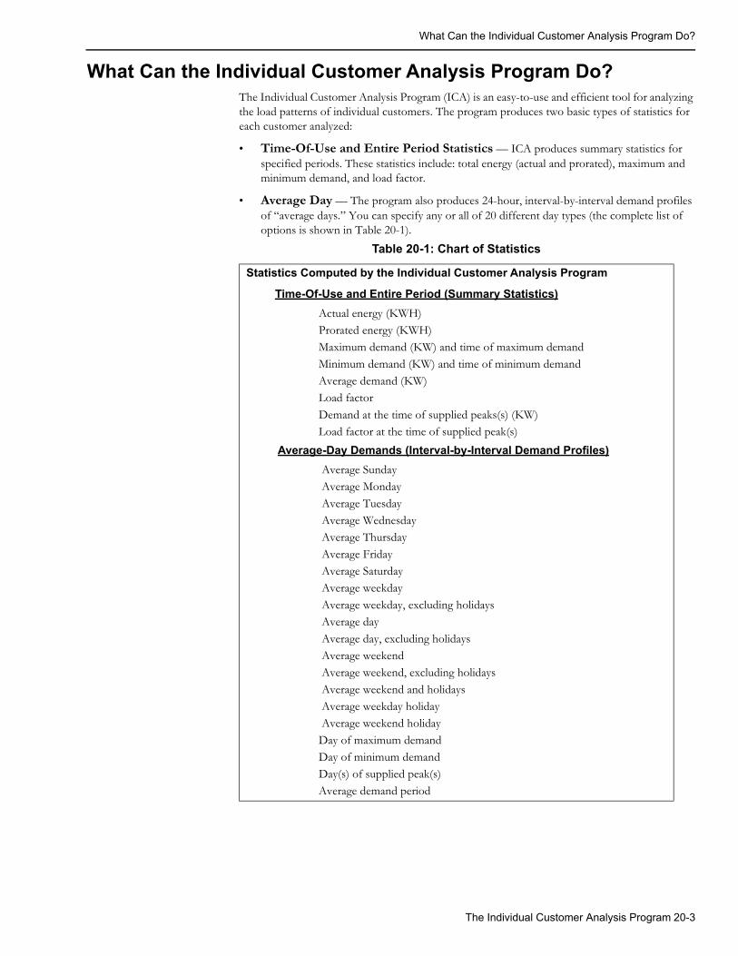
What Can the Individual Customer Analysis Program Do?
What Can the Individual Customer Analysis Program Do?The Individual Customer Analysis Program (ICA) is an easy-to-use and efficient tool for analyzing the load patterns of individual customers. The program produces two basic types of statistics for each customer analyzed:
• Time-Of-Use and Entire Period Statistics — ICA produces summary statistics for specified periods. These statistics include: total energy (actual and prorated), maximum and minimum demand, and load factor.
• Average Day — The program also produces 24-hour, interval-by-interval demand profiles of “average days.” You can specify any or all of 20 different day types (the complete list of options is shown in Table 20-1).
Table 20-1: Chart of Statistics
Statistics Computed by the Individual Customer Analysis Program
Time-Of-Use and Entire Period (Summary Statistics) Actual energy (KWH) Prorated energy (KWH) Maximum demand (KW) and time of maximum demand
Minimum demand (KW) and time of minimum demand Average demand (KW) Load factor
Demand at the time of supplied peaks(s) (KW) Load factor at the time of supplied peak(s)
Average-Day Demands (Interval-by-Interval Demand Profiles) Average Sunday Average Monday
Average Tuesday Average Wednesday Average Thursday
Average Friday Average Saturday Average weekday
Average weekday, excluding holidays Average day
Average day, excluding holidays Average weekend Average weekend, excluding holidays
Average weekend and holidays Average weekday holiday Average weekend holiday
Day of maximum demand Day of minimum demand Day(s) of supplied peak(s)
Average demand period
The Individual Customer Analysis Program 20-3
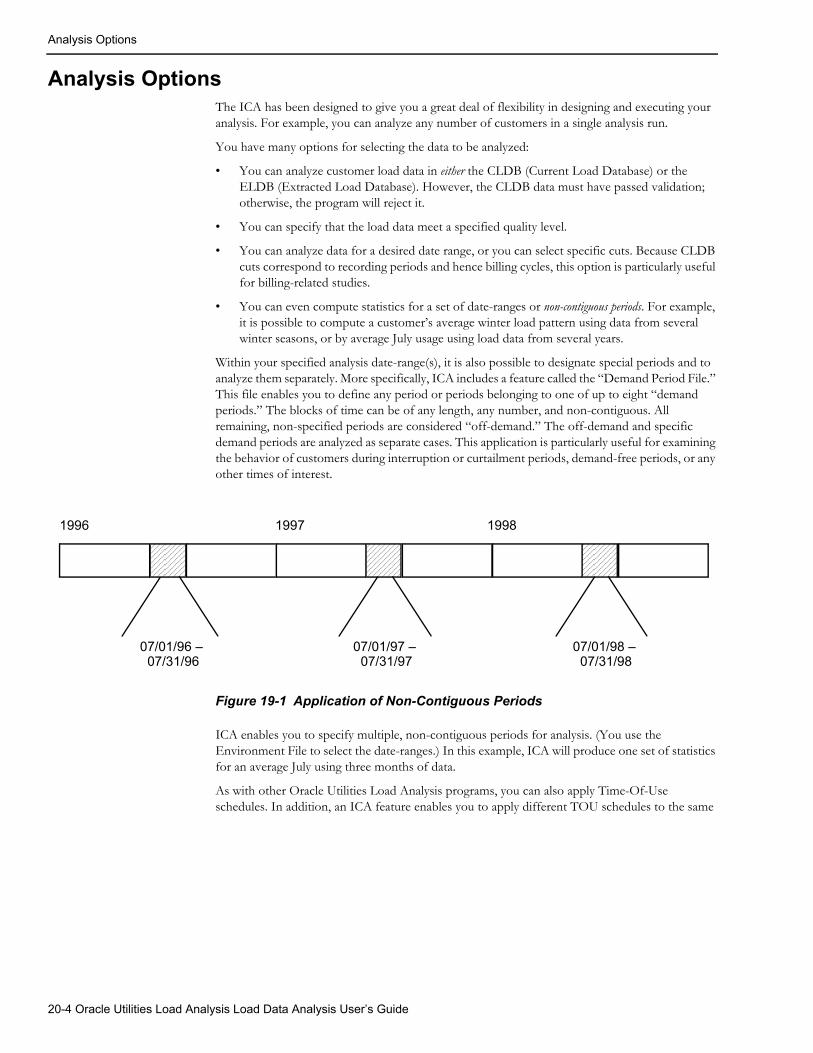
Analysis Options
Analysis OptionsThe ICA has been designed to give you a great deal of flexibility in designing and executing your analysis. For example, you can analyze any number of customers in a single analysis run.
You have many options for selecting the data to be analyzed:
• You can analyze customer load data in either the CLDB (Current Load Database) or the ELDB (Extracted Load Database). However, the CLDB data must have passed validation; otherwise, the program will reject it.
• You can specify that the load data meet a specified quality level.
• You can analyze data for a desired date range, or you can select specific cuts. Because CLDB cuts correspond to recording periods and hence billing cycles, this option is particularly useful for billing-related studies.
• You can even compute statistics for a set of date-ranges or non-contiguous periods. For example, it is possible to compute a customer’s average winter load pattern using data from several winter seasons, or by average July usage using load data from several years.
Within your specified analysis date-range(s), it is also possible to designate special periods and to analyze them separately. More specifically, ICA includes a feature called the “Demand Period File.” This file enables you to define any period or periods belonging to one of up to eight “demand periods.” The blocks of time can be of any length, any number, and non-contiguous. All remaining, non-specified periods are considered “off-demand.” The off-demand and specific demand periods are analyzed as separate cases. This application is particularly useful for examining the behavior of customers during interruption or curtailment periods, demand-free periods, or any other times of interest.
Figure 19-1 Application of Non-Contiguous Periods
ICA enables you to specify multiple, non-contiguous periods for analysis. (You use the Environment File to select the date-ranges.) In this example, ICA will produce one set of statistics for an average July using three months of data.
As with other Oracle Utilities Load Analysis programs, you can also apply Time-Of-Use schedules. In addition, an ICA feature enables you to apply different TOU schedules to the same
1996 1997 1998
07/01/97 – 07/31/97
07/01/96 – 07/31/96
07/01/98 – 07/31/98
20-4 Oracle Utilities Load Analysis Load Data Analysis User’s Guide
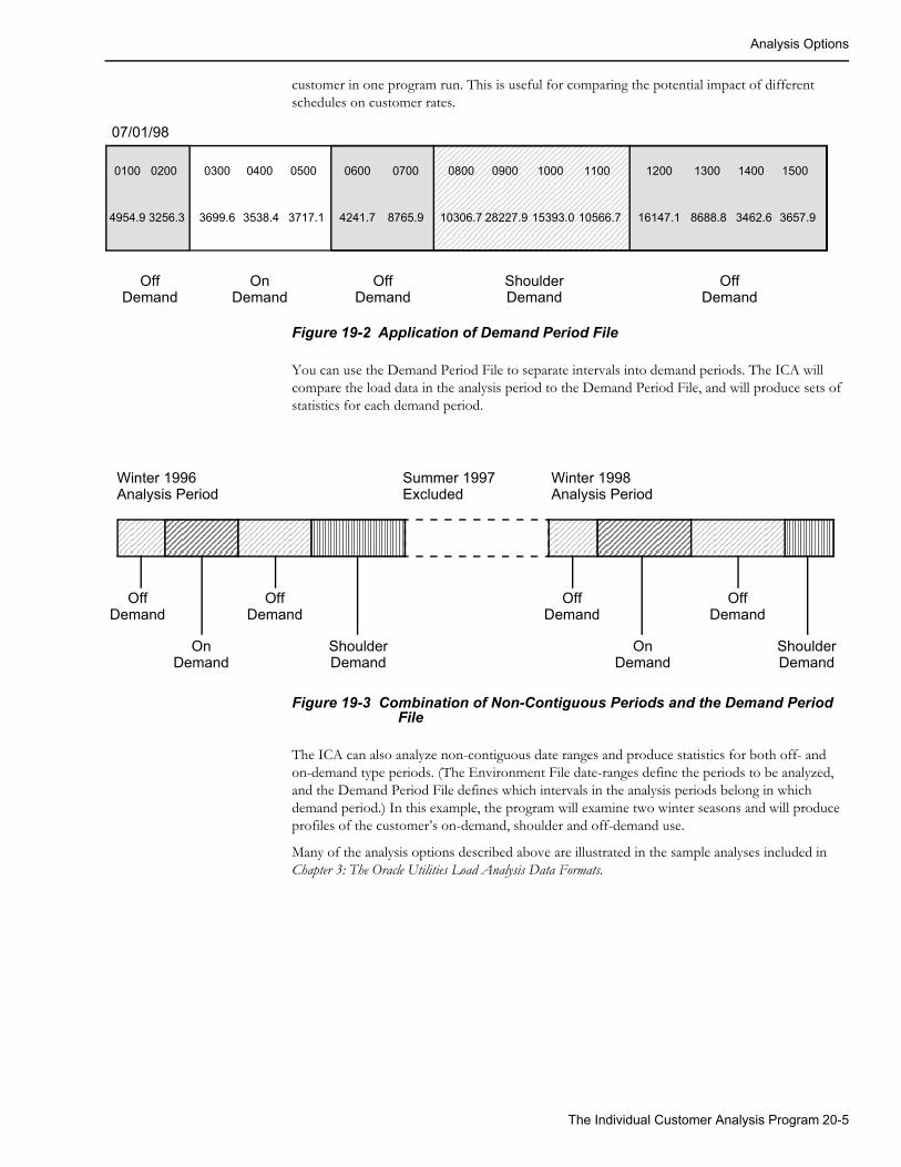
Analysis Options
customer in one program run. This is useful for comparing the potential impact of different schedules on customer rates.
Figure 19-2 Application of Demand Period File
You can use the Demand Period File to separate intervals into demand periods. The ICA will compare the load data in the analysis period to the Demand Period File, and will produce sets of statistics for each demand period.
Figure 19-3 Combination of Non-Contiguous Periods and the Demand Period File
The ICA can also analyze non-contiguous date ranges and produce statistics for both off- and on-demand type periods. (The Environment File date-ranges define the periods to be analyzed, and the Demand Period File defines which intervals in the analysis periods belong in which demand period.) In this example, the program will examine two winter seasons and will produce profiles of the customer’s on-demand, shoulder and off-demand use.
Many of the analysis options described above are illustrated in the sample analyses included in Chapter 3: The Oracle Utilities Load Analysis Data Formats.
07/01/98
0100 0200
4954.9 3256.3
0300 0400
3699.6 3538.4
0500
3717.1
0600 0700
4241.7 8765.9
0800 0900
10306.7 28227.9
1000
15393.0
1100
10566.7
1200 1300
16147.1 8688.8
1400
3462.6
1500
3657.9
OffDemand
OffDemand
OffDemand
OnDemand
ShoulderDemand
OffDemand
OffDemand
OffDemand
OffDemand
OnDemand
ShoulderDemand
OnDemand
ShoulderDemand
Winter 1996Analysis Period
Summer 1997Excluded
Winter 1998Analysis Period
The Individual Customer Analysis Program 20-5
Reporting
ReportingOnce the statistics have been calculated, you may report all of the results or only desired statistics. ICA can produce two types of reports for each customer analyzed: the Time-Of-Use Statistics Report and the Average Day Type Statistics Report. The reports are organized in a tabular format (columns and rows) similar to the Time Series Reporter format. You control the format — determining the order of the columns for Average Day Type Reports, and whether each new report begins on a separate page or each page contains as much information as possible. However, if average demand-period days are included, they are the last columns printed for a block.
Saving the Statistics for Further AnalysisYou can specify that the results be written to a sequential file for further analysis and reporting by non-Oracle Utilities programs. The format of these files is described in detail in Chapter 4: Oracle Utilities Load Analysis Mechanics.
Steps for Using the Individual Customer Analysis ProgramThe following provides a detailed, step-by-step explanation of how to use the Individual Customer Analysis Program. It explains how to set up or modify the required input files — the Environment, Control, Demand Period, Time-Of-Use, and Holiday files — and how to evaluate the output reports.
Individual Customer Analysis may be performed on load data in the Current Load Database (CLDB) that has passed validation, or on load data that has been extracted to the Extracted Load Database (ELDB).
Here is a brief list of the steps you will follow when analyzing load data with the Individual Customer Analysis Program. Later in this chapter these steps are explained in detail.
Note: The Y370 program supports pre-process key generator. See Using the Key Generator Preprocessor in a Control File on page 4-4 for more information.
Summary — Using Individual Customer Analysis
1. Create the Analysis Control File (TGY37A.CTL) — a list of the customers to be analyzed.
2. Create the Analysis Environment File (TGY37B.ENV)— a group of commands that you use to set analysis and reporting options.
3. Modify the Time-Of-Use Schedule File (TGY31D.TOU) if necessary.
4. Modify the Billing Cycle File (TGY23E.CYC) if necessary.
5. Modify the Demand Period File (TGY37E.DEM) if necessary.
6. Verify that the Holiday File (TGY31C.HOL) has been set up correctly.
7. Run the Individual Customer Analysis Program (Y370).
8. Check output:
Analysis reports
Individual Customer Statistics files.
20-6 Oracle Utilities Load Analysis Load Data Analysis User’s Guide
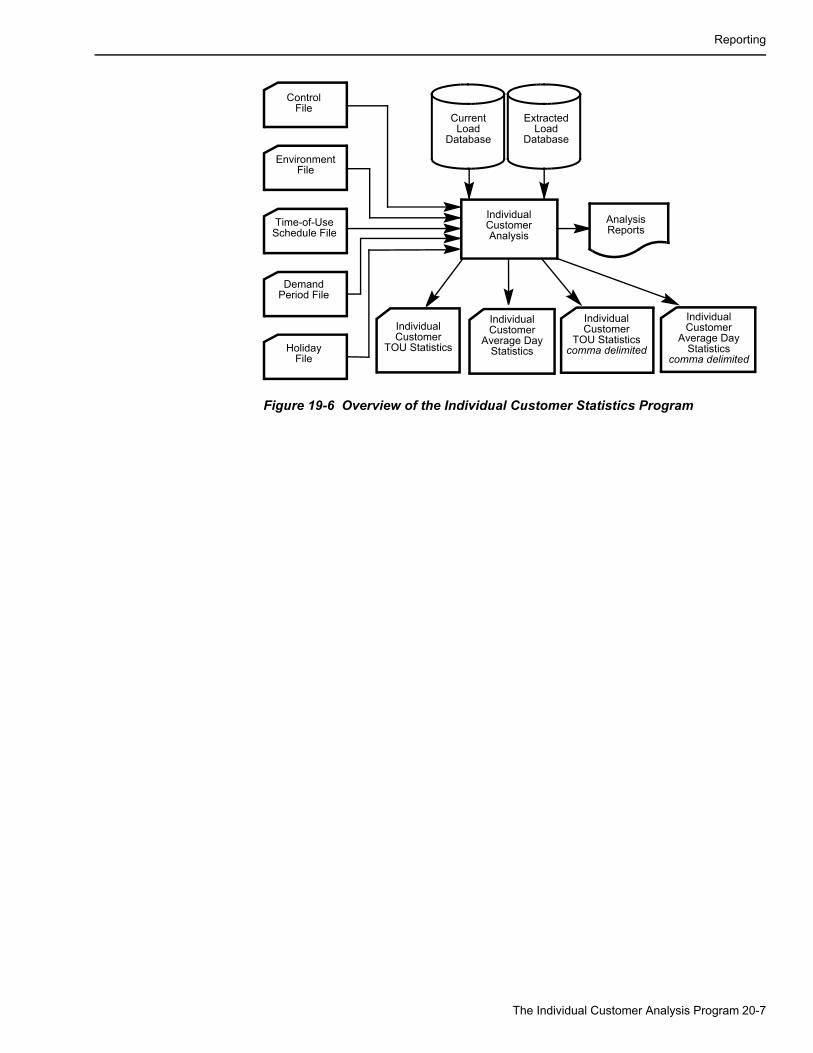
Reporting
Figure 19-6 Overview of the Individual Customer Statistics Program
ControlFile
EnvironmentFile
Time-of-UseSchedule File
DemandPeriod File
HolidayFile
ExtractedLoad
Database
IndividualCustomerAnalysis
IndividualCustomer
TOU Statistics
IndividualCustomer
Average DayStatistics
AnalysisReports
IndividualCustomer
TOU Statisticscomma delimited
Individual Customer
Average DayStatistics
comma delimited
CurrentLoad
Database
The Individual Customer Analysis Program 20-7
Reporting
Step 1: Create the Analysis Control File (TGY37A.CTL)The Analysis Control File is used to identify the customers you want to analyze, and to set two optional parameters (start-time and TOU Schedule).
You can type the file, or use the Key Generator or Customer Data Extraction Programs to construct it for you (these programs will select customer records that match user-defined criteria — see Chapter 10 in the Oracle Utilities Load Analysis Introductory Guide, Volume II).
Each record in the file must follow the format shown below. Input one record per line. You may input blank spaces or commas between elements in the command record, but do not input blanks between the lines.
customer-id chan1 [{±}chan2 [{±}chan3...[{±}chann ] ] ] [start-time | billing-cycle] [SCHedule [DEMand | t | 0] | SEAson [s | 0] ] [/*comment]
• customer-id — Input the Oracle Utilities Load Analysis customer-id.
• channel-number — Enter a channel-number or a combination of channels for that customer-id. A combination consists of two or more channels added or subtracted to represent the total customer load (e.g., 1+2-4 is the sum of channels 1 and 2 minus channel 4, a co-generation unit).
Important Note: If you combine multiple channels for a customer-id and specify a start-time in the record (see below), each channel of data must have the same start- and stop-time.
Note: If you want to combine multiple IDs for a large individual customer into a single record, you cannot do it in the Analysis Control File — you must use the Oracle Utilities Load Analysis Transformation Program.
• start-time — Use this optional parameter if you want to analyze customer load data by cuts. Input a cut’s start-time in either the “mmddyyhhmmss” or “mm/dd/yy-hh:mm:ss” format.
This start-time parameter makes it possible to: a) analyze cuts, and b) specify a different start-time for each customer in the Control File. (If you want to apply the same analysis period to all customers in the Control File, use the Environment File Date Command instead.)
Note: If you do use the start-time parameter, you must supply a start-time for every customer in the Control File.
If you do not specify a start-time, the ICA program will use the date-range(s) specified in the Environment File.
• billing cycle — This optional parameter makes it possible to specify a different date range for each customer in the control file, rather than the start-time of a specific cut. You do this by specifying an integer from 1 to 99 representing one of the billing cycles defined in the Billing Cycle File. Each record in that file contains a billing cycle number, and the start and stop times that are defined for that cycle. If you specify a billing cycle for a customer in the Control File, the program will analyze that customer’s load data over the date range defined for that cycle in the Billing Cycle File.
Important Note: If, as is often the case, a billing cycle start-time in the Billing Cycle File is defined as a date only (without hours, minutes, and seconds), the program will assume a start time of 00:00:00; if a billing cycle stop-time is defined as a date only, the program will assume a stop time of 23:59:59.
SCHedule — Use this optional parameter to specify a Time-of-Use Schedule for the TOU calculations, or to specify that the Demand Period File be applied to the customer analysis. Enter a value “t ” (where t = the number of the desired schedule in the TOU Schedule file), or “DEM” to apply the Demand Period File. (The TOU Schedule File and the Demand Period files are explained further later in this chapter.) You must include keyword SCH before the schedule number or the DEM keyword.
20-8 Oracle Utilities Load Analysis Load Data Analysis User’s Guide
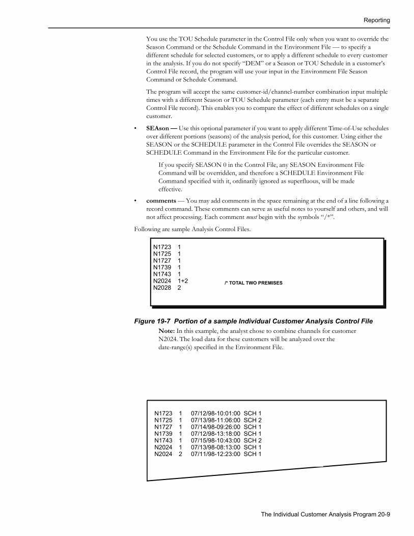
Reporting
You use the TOU Schedule parameter in the Control File only when you want to override the Season Command or the Schedule Command in the Environment File — to specify a different schedule for selected customers, or to apply a different schedule to every customer in the analysis. If you do not specify “DEM” or a Season or TOU Schedule in a customer’s Control File record, the program will use your input in the Environment File Season Command or Schedule Command.
The program will accept the same customer-id/channel-number combination input multiple times with a different Season or TOU Schedule parameter (each entry must be a separate Control File record). This enables you to compare the effect of different schedules on a single customer.
• SEAson — Use this optional parameter if you want to apply different Time-of-Use schedules over different portions (seasons) of the analysis period, for this customer. Using either the SEASON or the SCHEDULE parameter in the Control File overrides the SEASON or SCHEDULE Command in the Environment File for the particular customer.
If you specify SEASON 0 in the Control File, any SEASON Environment File Command will be overridden, and therefore a SCHEDULE Environment File Command specified with it, ordinarily ignored as superfluous, will be made effective.
• comments — You may add comments in the space remaining at the end of a line following a record command. These comments can serve as useful notes to yourself and others, and will not affect processing. Each comment must begin with the symbols “/*”.
Following are sample Analysis Control Files.
Figure 19-7 Portion of a sample Individual Customer Analysis Control FileNote: In this example, the analyst chose to combine channels for customer N2024. The load data for these customers will be analyzed over the date-range(s) specified in the Environment File.
N1723 1N1725 1N1727 1N1739 1N1743 1N2024 1+2N2028 2
/* TOTAL TWO PREMISES
N1723 1 07/12/98-10:01:00 SCH 1N1725 1 07/13/98-11:06:00 SCH 2N1727 1 07/14/98-09:26:00 SCH 1N1739 1 07/12/98-13:18:00 SCH 1N1743 1 07/15/98-10:43:00 SCH 2N2024 1 07/13/98-08:13:00 SCH 1N2024 2 07/11/98-12:23:00 SCH 1
The Individual Customer Analysis Program 20-9
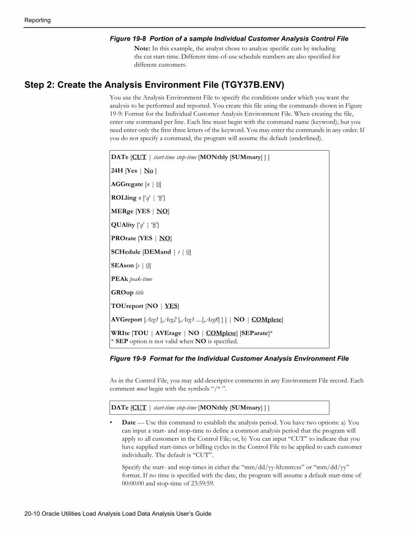
Reporting
Figure 19-8 Portion of a sample Individual Customer Analysis Control FileNote: In this example, the analyst chose to analyze specific cuts by including the cut start-time. Different time-of-use schedule numbers are also specified for different customers.
Step 2: Create the Analysis Environment File (TGY37B.ENV)You use the Analysis Environment File to specify the conditions under which you want the analysis to be performed and reported. You create this file using the commands shown in Figure 19-9: Format for the Individual Customer Analysis Environment File. When creating the file, enter one command per line. Each line must begin with the command name (keyword); but you need enter only the first three letters of the keyword. You may enter the commands in any order. If you do not specify a command, the program will assume the default (underlined).
Figure 19-9 Format for the Individual Customer Analysis Environment File
As in the Control File, you may add descriptive comments in any Environment File record. Each comment must begin with the symbols “/* ”.
• Date — Use this command to establish the analysis period. You have two options: a) You can input a start- and stop-time to define a common analysis period that the program will apply to all customers in the Control File; or, b) You can input “CUT” to indicate that you have supplied start-times or billing cycles in the Control File to be applied to each customer individually. The default is “CUT”.
Specify the start- and stop-times in either the “mm/dd/yy-hh:mm:ss” or “mm/dd/yy” format. If no time is specified with the date, the program will assume a default start-time of 00:00:00 and stop-time of 23:59:59.
DATe [CUT | start-time stop-time [MONthly [SUMmary] ] ]
24H [Yes | No ]
AGGregate [n | 0]
ROLling n [‘q’ | ‘8’]
MERge [YES | NO]
QUAlity [‘q’ | ‘8’]
PROrate [YES | NO]
SCHedule [DEMand | t | 0]
SEAson [s | 0]
PEAk peak-time
GROup title
TOUreport [NO | YES]
AVGreport [Avg1 [,Avg2 [,Avg3 ....[,Avg8] ] ] | NO | COMplete]
WRIte [TOU | AVErage | NO | COMplete] [SEParate]* * SEP option is not valid when NO is specified.
DATe [CUT | start-time stop-time [MONthly [SUMmary] ] ]
20-10 Oracle Utilities Load Analysis Load Data Analysis User’s Guide
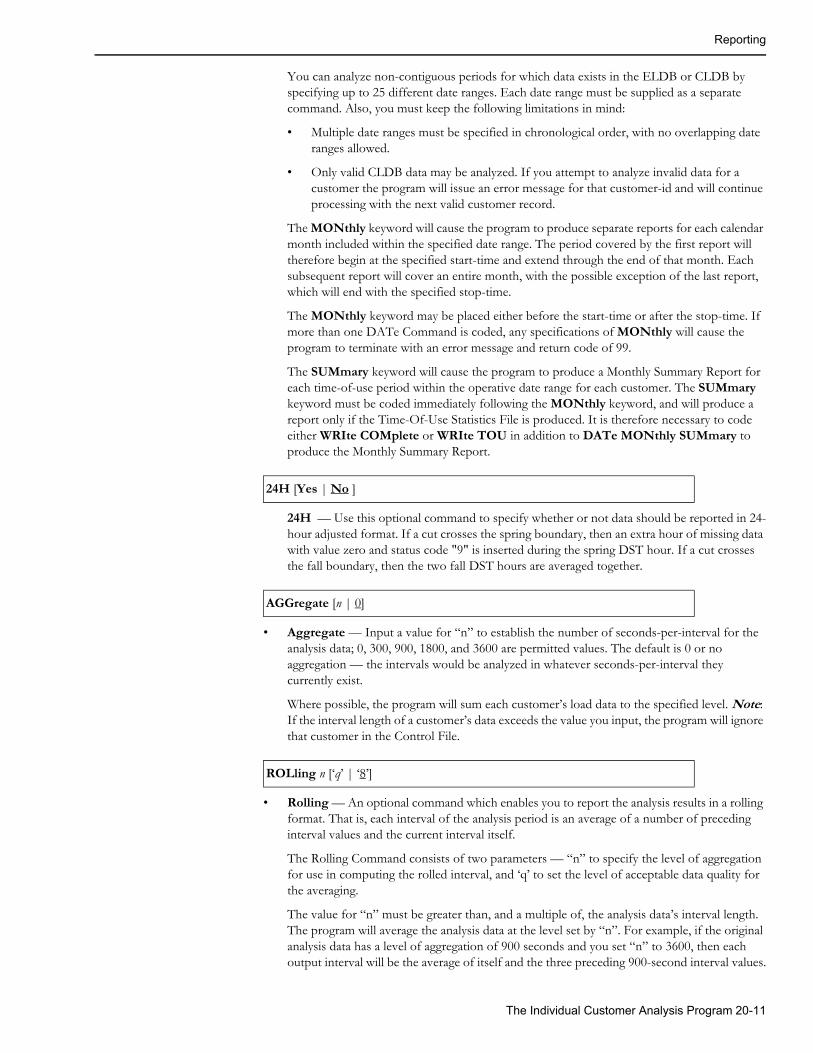
Reporting
You can analyze non-contiguous periods for which data exists in the ELDB or CLDB by specifying up to 25 different date ranges. Each date range must be supplied as a separate command. Also, you must keep the following limitations in mind:
• Multiple date ranges must be specified in chronological order, with no overlapping date ranges allowed.
• Only valid CLDB data may be analyzed. If you attempt to analyze invalid data for a customer the program will issue an error message for that customer-id and will continue processing with the next valid customer record.
The MONthly keyword will cause the program to produce separate reports for each calendar month included within the specified date range. The period covered by the first report will therefore begin at the specified start-time and extend through the end of that month. Each subsequent report will cover an entire month, with the possible exception of the last report, which will end with the specified stop-time.
The MONthly keyword may be placed either before the start-time or after the stop-time. If more than one DATe Command is coded, any specifications of MONthly will cause the program to terminate with an error message and return code of 99.
The SUMmary keyword will cause the program to produce a Monthly Summary Report for each time-of-use period within the operative date range for each customer. The SUMmary keyword must be coded immediately following the MONthly keyword, and will produce a report only if the Time-Of-Use Statistics File is produced. It is therefore necessary to code either WRIte COMplete or WRIte TOU in addition to DATe MONthly SUMmary to produce the Monthly Summary Report.
24H — Use this optional command to specify whether or not data should be reported in 24-hour adjusted format. If a cut crosses the spring boundary, then an extra hour of missing data with value zero and status code "9" is inserted during the spring DST hour. If a cut crosses the fall boundary, then the two fall DST hours are averaged together.
• Aggregate — Input a value for “n” to establish the number of seconds-per-interval for the analysis data; 0, 300, 900, 1800, and 3600 are permitted values. The default is 0 or no aggregation — the intervals would be analyzed in whatever seconds-per-interval they currently exist.
Where possible, the program will sum each customer’s load data to the specified level. Note: If the interval length of a customer’s data exceeds the value you input, the program will ignore that customer in the Control File.
• Rolling — An optional command which enables you to report the analysis results in a rolling format. That is, each interval of the analysis period is an average of a number of preceding interval values and the current interval itself.
The Rolling Command consists of two parameters — “n” to specify the level of aggregation for use in computing the rolled interval, and ‘q’ to set the level of acceptable data quality for the averaging.
The value for “n” must be greater than, and a multiple of, the analysis data’s interval length. The program will average the analysis data at the level set by “n”. For example, if the original analysis data has a level of aggregation of 900 seconds and you set “n” to 3600, then each output interval will be the average of itself and the three preceding 900-second interval values.
24H [Yes | No ]
AGGregate [n | 0]
ROLling n [‘q’ | ‘8’]
The Individual Customer Analysis Program 20-11
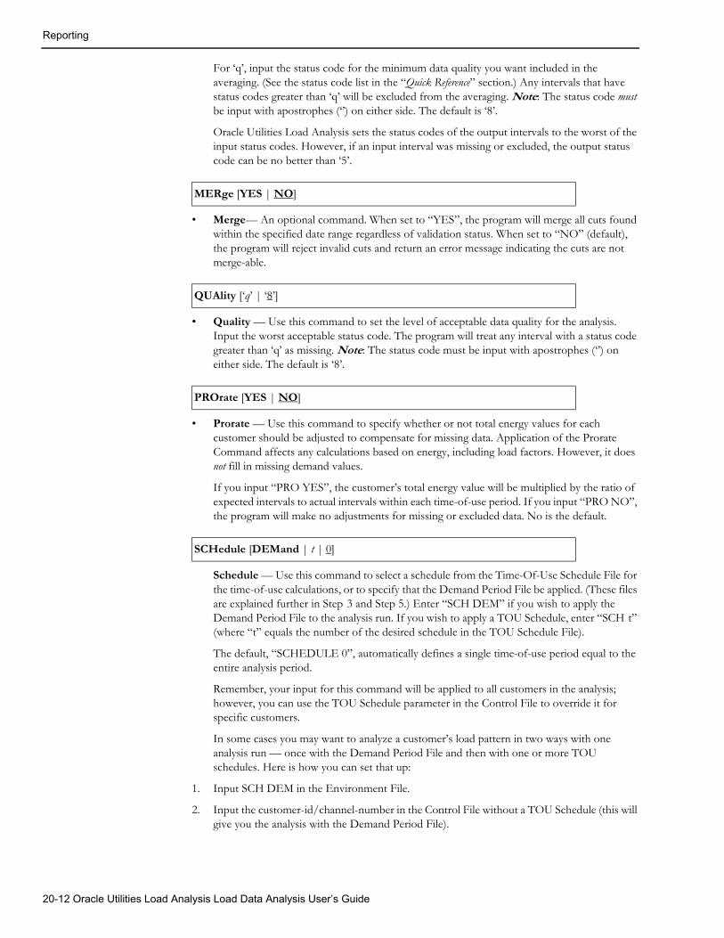
Reporting
For ‘q’, input the status code for the minimum data quality you want included in the averaging. (See the status code list in the “Quick Reference” section.) Any intervals that have status codes greater than ‘q’ will be excluded from the averaging. Note: The status code must be input with apostrophes (‘’) on either side. The default is ‘8’.
Oracle Utilities Load Analysis sets the status codes of the output intervals to the worst of the input status codes. However, if an input interval was missing or excluded, the output status code can be no better than ‘5’.
• Merge— An optional command. When set to “YES”, the program will merge all cuts found within the specified date range regardless of validation status. When set to “NO” (default), the program will reject invalid cuts and return an error message indicating the cuts are not merge-able.
• Quality — Use this command to set the level of acceptable data quality for the analysis. Input the worst acceptable status code. The program will treat any interval with a status code greater than ‘q’ as missing. Note: The status code must be input with apostrophes (‘’) on either side. The default is ‘8’.
• Prorate — Use this command to specify whether or not total energy values for each customer should be adjusted to compensate for missing data. Application of the Prorate Command affects any calculations based on energy, including load factors. However, it does not fill in missing demand values.
If you input “PRO YES”, the customer’s total energy value will be multiplied by the ratio of expected intervals to actual intervals within each time-of-use period. If you input “PRO NO”, the program will make no adjustments for missing or excluded data. No is the default.
Schedule — Use this command to select a schedule from the Time-Of-Use Schedule File for the time-of-use calculations, or to specify that the Demand Period File be applied. (These files are explained further in Step 3 and Step 5.) Enter “SCH DEM” if you wish to apply the Demand Period File to the analysis run. If you wish to apply a TOU Schedule, enter “SCH t” (where “t” equals the number of the desired schedule in the TOU Schedule File).
The default, “SCHEDULE 0”, automatically defines a single time-of-use period equal to the entire analysis period.
Remember, your input for this command will be applied to all customers in the analysis; however, you can use the TOU Schedule parameter in the Control File to override it for specific customers.
In some cases you may want to analyze a customer’s load pattern in two ways with one analysis run — once with the Demand Period File and then with one or more TOU schedules. Here is how you can set that up:
1. Input SCH DEM in the Environment File.
2. Input the customer-id/channel-number in the Control File without a TOU Schedule (this will give you the analysis with the Demand Period File).
MERge [YES | NO]
QUAlity [‘q’ | ‘8’]
PROrate [YES | NO]
SCHedule [DEMand | t | 0]
20-12 Oracle Utilities Load Analysis Load Data Analysis User’s Guide
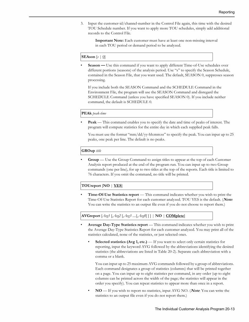
Reporting
3. Input the customer-id/channel-number in the Control File again, this time with the desired TOU Schedule number. If you want to apply more TOU schedules, simply add additional records to the Control File.
Important Note: Each customer must have at least one non-missing interval in each TOU period or demand period to be analyzed.
• Season — Use this command if you want to apply different Time-of-Use schedules over different portions (seasons) of the analysis period. Use “s” to specify the Season Schedule, contained in the Season File, that you want used. The default, SEASON 0, suppresses season processing.
If you include both the SEASON Command and the SCHEDULE Command in the Environment File, the program will use the SEASON Command and disregard the SCHEDULE Command (unless you have specified SEASON 0). If you include neither command, the default is SCHEDULE 0.
• Peak — This command enables you to specify the date and time of peaks of interest. The program will compute statistics for the entire day in which each supplied peak falls.
You must use the format “mm/dd/yy-hh:mm:ss” to specify the peak. You can input up to 25 peaks, one peak per line. The default is no peaks.
• Group — Use the Group Command to assign titles to appear at the top of each Customer Analysis report produced at the end of the program run. You can input up to two Group commands (one per line), for up to two titles at the top of the reports. Each title is limited to 76 characters. If you omit the command, no title will be printed.
• Time-Of-Use Statistics report — This command indicates whether you wish to print the Time-Of-Use Statistics Report for each customer analyzed. TOU YES is the default. (Note: You can write the statistics to an output file even if you do not choose to report them.)
• Average Day-Type Statistics report — This command indicates whether you wish to print the Average Day-Type Statistics Report for each customer analyzed. You may print all of the statistics calculated, none of the statistics, or just selected ones.
• Selected statistics (Avg 1, etc.) — If you want to select only certain statistics for reporting, input the keyword AVG followed by the abbreviations identifying the desired statistics (the abbreviations are listed in Table 20-2). Separate each abbreviation with a comma or a blank.
You can input up to 25 maximum AVG commands followed by a group of abbreviations. Each command designates a group of statistics (columns) that will be printed together on a page. You can input up to eight statistics per command, in any order (up to eight columns can be printed across the width of the page; the statistics will appear in the order you specify). You can repeat statistics to appear more than once in a report.
• NO — If you wish to report no statistics, input AVG NO. (Note: You can write the statistics to an output file even if you do not report them.)
SEAson [s | 0]
PEAk peak-time
GROup title
TOUreport [NO | YES]
AVGreport [Avg1 [,Avg2 [,Avg3 ....[,Avg8] ] ] | NO | COMplete]
The Individual Customer Analysis Program 20-13

Reporting
• COM — If you wish to report all 20 average-day-type statistics, input AVG COM. This is the default. Do not input any selected statistics if you use the COM option.
*The Average Demand Period statistic may be calculated and reported if you have a Demand Period File, regardless of whether or not you apply a TOU Schedule to the analysis.
• Write — Use this command to determine which, if any, statistics should be written to output files. (The formats of these files are explained in Chapter 4: Oracle Utilities Load Analysis Mechanics.)
• TOU — Input WRI TOU if you wish to output just the Time-Of-Use type statistics.
• AVE — Input WRI AVE if you wish to output just the Average Day-Type statistics.
• NO — Input WRI NO if no statistical records should be written out.
• COMplete — Input WRI COM to write all statistical records produced by the analysis run to the output files. This is the default.
• SEParate — Input SEP after the above WRI commands to produce a delimited file (i.e., WRI COM SEP). Note: SEP is not valid with the WRI NO Command.
• HEAder — Input HEA after the above WRI commands to include headers in the output file.
Table 20-2: Abbreviations for specifying Average Day Type Statistics in the
Environment File’s AVGREPORT Command
Average Day Type Statistics AbbreviationsADADXWDWDXWNWNXWEHWDHWNHSUNMONTUEWEDTHUFRISATMAXMINDEMP01-P25
Average dayAverage day, excluding holidaysAverage weekdayAverage weekday, excluding holidaysAverage weekendAverage weekend, excluding holidaysAverage weekend and holidaysAverage weekday holidayAverage weekend holidayAverage SundayAverage MondayAverage TuesdayAverage WednesdayAverage ThursdayAverage FridayAverage SaturdayDay of MaximumDay of MinimumAverage Demand Period*Day of supplied peak X
WRIte [TOU | AVErage | NO | COMplete] [SEParate]* [HEAder]* SEP option is not valid when NO is specified.
20-14 Oracle Utilities Load Analysis Load Data Analysis User’s Guide
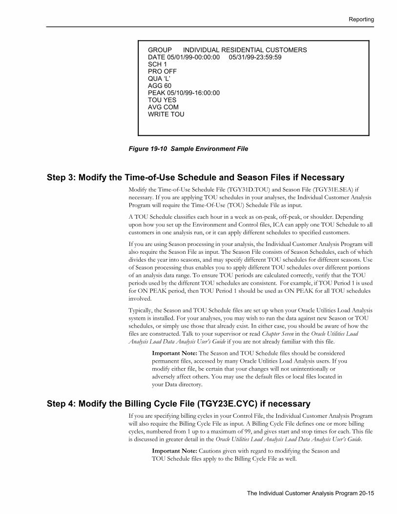
Reporting
Figure 19-10 Sample Environment File
Step 3: Modify the Time-of-Use Schedule and Season Files if NecessaryModify the Time-of-Use Schedule File (TGY31D.TOU) and Season File (TGY31E.SEA) if necessary. If you are applying TOU schedules in your analyses, the Individual Customer Analysis Program will require the Time-Of-Use (TOU) Schedule File as input.
A TOU Schedule classifies each hour in a week as on-peak, off-peak, or shoulder. Depending upon how you set up the Environment and Control files, ICA can apply one TOU Schedule to all customers in one analysis run, or it can apply different schedules to specified customers.
If you are using Season processing in your analysis, the Individual Customer Analysis Program will also require the Season File as input. The Season File consists of Season Schedules, each of which divides the year into seasons, and may specify different TOU schedules for different seasons. Use of Season processing thus enables you to apply different TOU schedules over different portions of an analysis data range. To ensure TOU periods are calculated correctly, verify that the TOU periods used by the different TOU schedules are consistent. For example, if TOU Period 1 is used for ON PEAK period, then TOU Period 1 should be used as ON PEAK for all TOU schedules involved.
Typically, the Season and TOU Schedule files are set up when your Oracle Utilities Load Analysis system is installed. For your analyses, you may wish to run the data against new Season or TOU schedules, or simply use those that already exist. In either case, you should be aware of how the files are constructed. Talk to your supervisor or read Chapter Seven in the Oracle Utilities Load Analysis Load Data Analysis User’s Guide if you are not already familiar with this file.
Important Note: The Season and TOU Schedule files should be considered permanent files, accessed by many Oracle Utilities Load Analysis users. If you modify either file, be certain that your changes will not unintentionally or adversely affect others. You may use the default files or local files located in your Data directory.
Step 4: Modify the Billing Cycle File (TGY23E.CYC) if necessary If you are specifying billing cycles in your Control File, the Individual Customer Analysis Program will also require the Billing Cycle File as input. A Billing Cycle File defines one or more billing cycles, numbered from 1 up to a maximum of 99, and gives start and stop times for each. This file is discussed in greater detail in the Oracle Utilities Load Analysis Load Data Analysis User’s Guide.
Important Note: Cautions given with regard to modifying the Season and TOU Schedule files apply to the Billing Cycle File as well.
GROUP INDIVIDUAL RESIDENTIAL CUSTOMERSDATE 05/01/99-00:00:00 05/31/99-23:59:59SCH 1PRO OFFQUA ‘L’AGG 60PEAK 05/10/99-16:00:00TOU YESAVG COMWRITE TOU
The Individual Customer Analysis Program 20-15
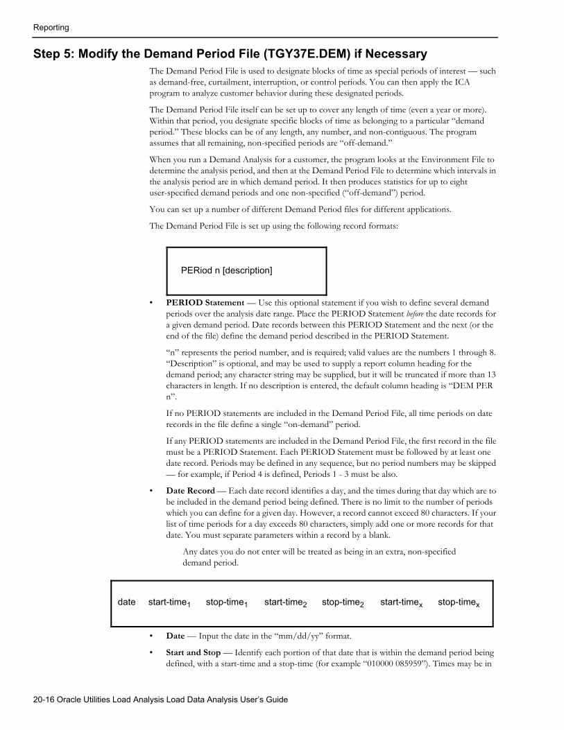
Reporting
Step 5: Modify the Demand Period File (TGY37E.DEM) if NecessaryThe Demand Period File is used to designate blocks of time as special periods of interest — such as demand-free, curtailment, interruption, or control periods. You can then apply the ICA program to analyze customer behavior during these designated periods.
The Demand Period File itself can be set up to cover any length of time (even a year or more). Within that period, you designate specific blocks of time as belonging to a particular “demand period.” These blocks can be of any length, any number, and non-contiguous. The program assumes that all remaining, non-specified periods are “off-demand.”
When you run a Demand Analysis for a customer, the program looks at the Environment File to determine the analysis period, and then at the Demand Period File to determine which intervals in the analysis period are in which demand period. It then produces statistics for up to eight user-specified demand periods and one non-specified (“off-demand”) period.
You can set up a number of different Demand Period files for different applications.
The Demand Period File is set up using the following record formats:
• PERIOD Statement — Use this optional statement if you wish to define several demand periods over the analysis date range. Place the PERIOD Statement before the date records for a given demand period. Date records between this PERIOD Statement and the next (or the end of the file) define the demand period described in the PERIOD Statement.
“n” represents the period number, and is required; valid values are the numbers 1 through 8. “Description” is optional, and may be used to supply a report column heading for the demand period; any character string may be supplied, but it will be truncated if more than 13 characters in length. If no description is entered, the default column heading is “DEM PER n”.
If no PERIOD statements are included in the Demand Period File, all time periods on date records in the file define a single “on-demand” period.
If any PERIOD statements are included in the Demand Period File, the first record in the file must be a PERIOD Statement. Each PERIOD Statement must be followed by at least one date record. Periods may be defined in any sequence, but no period numbers may be skipped — for example, if Period 4 is defined, Periods 1 - 3 must be also.
• Date Record — Each date record identifies a day, and the times during that day which are to be included in the demand period being defined. There is no limit to the number of periods which you can define for a given day. However, a record cannot exceed 80 characters. If your list of time periods for a day exceeds 80 characters, simply add one or more records for that date. You must separate parameters within a record by a blank.
Any dates you do not enter will be treated as being in an extra, non-specified demand period.
• Date — Input the date in the “mm/dd/yy” format.
• Start and Stop — Identify each portion of that date that is within the demand period being defined, with a start-time and a stop-time (for example “010000 085959”). Times may be in
PERiod n [description]
date start-time1 stop-time1 start-time2 stop-time2 start-timex stop-timex
20-16 Oracle Utilities Load Analysis Load Data Analysis User’s Guide
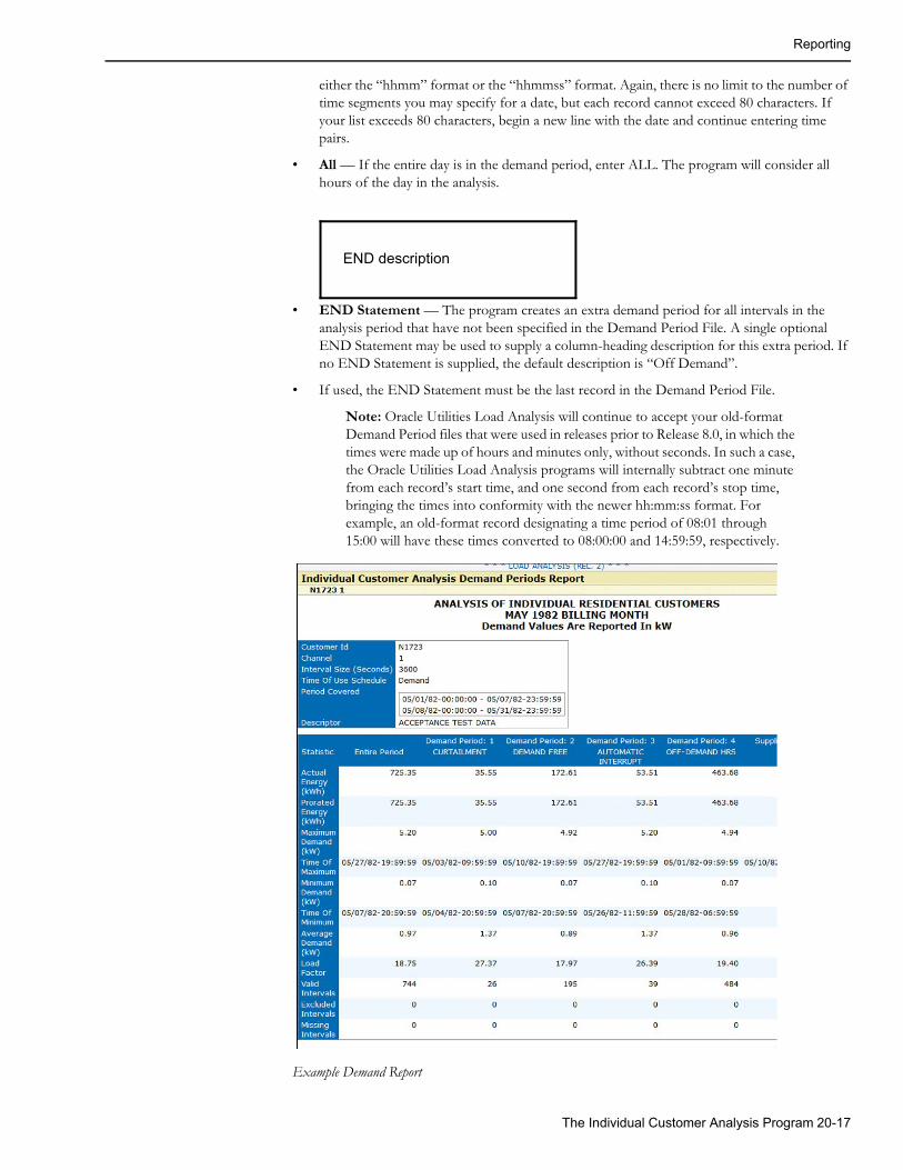
Reporting
either the “hhmm” format or the “hhmmss” format. Again, there is no limit to the number of time segments you may specify for a date, but each record cannot exceed 80 characters. If your list exceeds 80 characters, begin a new line with the date and continue entering time pairs.
• All — If the entire day is in the demand period, enter ALL. The program will consider all hours of the day in the analysis.
• END Statement — The program creates an extra demand period for all intervals in the analysis period that have not been specified in the Demand Period File. A single optional END Statement may be used to supply a column-heading description for this extra period. If no END Statement is supplied, the default description is “Off Demand”.
• If used, the END Statement must be the last record in the Demand Period File.
Note: Oracle Utilities Load Analysis will continue to accept your old-format Demand Period files that were used in releases prior to Release 8.0, in which the times were made up of hours and minutes only, without seconds. In such a case, the Oracle Utilities Load Analysis programs will internally subtract one minute from each record’s start time, and one second from each record’s stop time, bringing the times into conformity with the newer hh:mm:ss format. For example, an old-format record designating a time period of 08:01 through 15:00 will have these times converted to 08:00:00 and 14:59:59, respectively.
Example Demand Report
END description
The Individual Customer Analysis Program 20-17
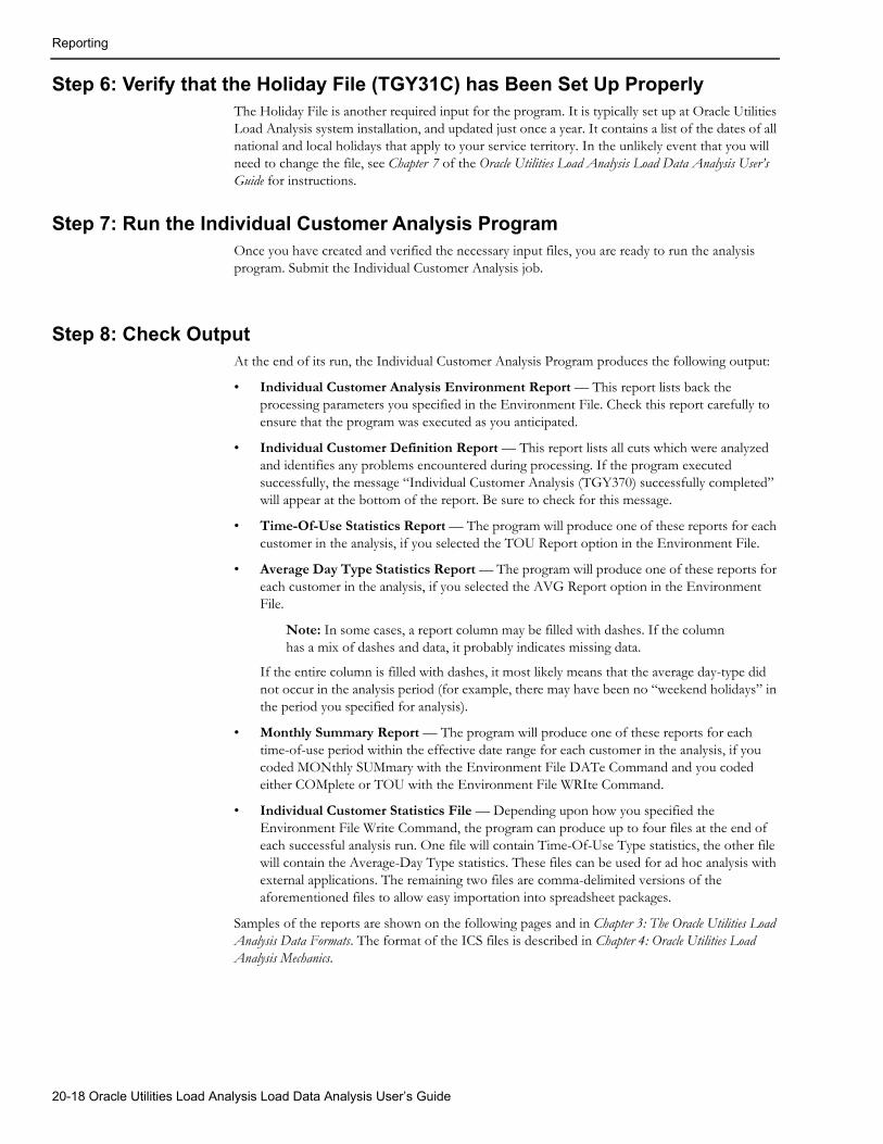
Reporting
Step 6: Verify that the Holiday File (TGY31C) has Been Set Up ProperlyThe Holiday File is another required input for the program. It is typically set up at Oracle Utilities Load Analysis system installation, and updated just once a year. It contains a list of the dates of all national and local holidays that apply to your service territory. In the unlikely event that you will need to change the file, see Chapter 7 of the Oracle Utilities Load Analysis Load Data Analysis User’s Guide for instructions.
Step 7: Run the Individual Customer Analysis ProgramOnce you have created and verified the necessary input files, you are ready to run the analysis program. Submit the Individual Customer Analysis job.
Step 8: Check OutputAt the end of its run, the Individual Customer Analysis Program produces the following output:
• Individual Customer Analysis Environment Report — This report lists back the processing parameters you specified in the Environment File. Check this report carefully to ensure that the program was executed as you anticipated.
• Individual Customer Definition Report — This report lists all cuts which were analyzed and identifies any problems encountered during processing. If the program executed successfully, the message “Individual Customer Analysis (TGY370) successfully completed” will appear at the bottom of the report. Be sure to check for this message.
• Time-Of-Use Statistics Report — The program will produce one of these reports for each customer in the analysis, if you selected the TOU Report option in the Environment File.
• Average Day Type Statistics Report — The program will produce one of these reports for each customer in the analysis, if you selected the AVG Report option in the Environment File.
Note: In some cases, a report column may be filled with dashes. If the column has a mix of dashes and data, it probably indicates missing data.
If the entire column is filled with dashes, it most likely means that the average day-type did not occur in the analysis period (for example, there may have been no “weekend holidays” in the period you specified for analysis).
• Monthly Summary Report — The program will produce one of these reports for each time-of-use period within the effective date range for each customer in the analysis, if you coded MONthly SUMmary with the Environment File DATe Command and you coded either COMplete or TOU with the Environment File WRIte Command.
• Individual Customer Statistics File — Depending upon how you specified the Environment File Write Command, the program can produce up to four files at the end of each successful analysis run. One file will contain Time-Of-Use Type statistics, the other file will contain the Average-Day Type statistics. These files can be used for ad hoc analysis with external applications. The remaining two files are comma-delimited versions of the aforementioned files to allow easy importation into spreadsheet packages.
Samples of the reports are shown on the following pages and in Chapter 3: The Oracle Utilities Load Analysis Data Formats. The format of the ICS files is described in Chapter 4: Oracle Utilities Load Analysis Mechanics.
20-18 Oracle Utilities Load Analysis Load Data Analysis User’s Guide
Sample Applications of the Individual Customer Analysis Program
Sample Applications of the Individual Customer Analysis ProgramThe following includes four sample analyses. They are intended to show you how to set up the input files and evaluate the output, as well as to give you a broader understanding of how the program’s capabilities can be applied in different situations. The examples illustrate analysis of:
• Non-contiguous periods
• CLDB cuts
• Curtailment periods
• TOU periods
The samples on the following pages highlight some of the key features of the ICA, and may suggest ways in which you can apply the program to your operations.
Here is a list of the four examples and what each is intended to illustrate:
For each example, we will look at the input files and the output reports. While each analysis is performed on a group of customers, we will show the output reports for just one representative customer, since the report format is the same for every customer in the analysis.
Example A — how to set up an analysis of customer load data over non-contiguous calendar periods (in this case, three Julys).
Example B — how to analyze a series of CLDB cuts that correspond to customer billing cycles.
Example C — how to use the Demand Period File to examine customer usage during Curtailment Periods.
Example D — how to limit output to just one type of statistic.
The Individual Customer Analysis Program 20-19
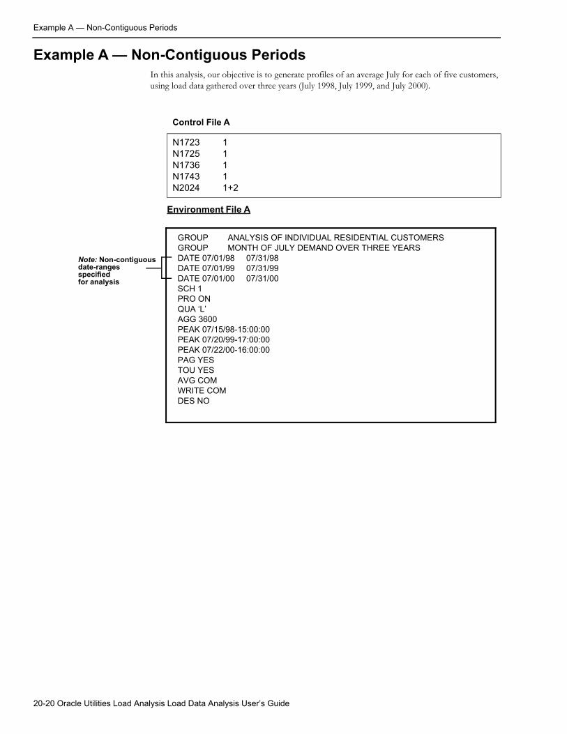
Example A — Non-Contiguous Periods
Example A — Non-Contiguous PeriodsIn this analysis, our objective is to generate profiles of an average July for each of five customers, using load data gathered over three years (July 1998, July 1999, and July 2000).
Control File A
N1723 1N1725 1N1736 1N1743 1N2024 1+2
GROUP ANALYSIS OF INDIVIDUAL RESIDENTIAL CUSTOMERSGROUP MONTH OF JULY DEMAND OVER THREE YEARSDATE 07/01/98 07/31/98DATE 07/01/99 07/31/99DATE 07/01/00 07/31/00SCH 1PRO ONQUA ‘L’AGG 3600PEAK 07/15/98-15:00:00PEAK 07/20/99-17:00:00PEAK 07/22/00-16:00:00PAG YESTOU YESAVG COMWRITE COMDES NO
Environment File A
Note: Non-contiguousdate-rangesspecifiedfor analysis
20-20 Oracle Utilities Load Analysis Load Data Analysis User’s Guide
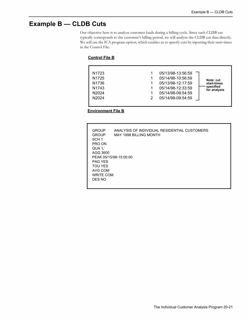
Example B — CLDB Cuts
Example B — CLDB CutsOur objective here is to analyze customer loads during a billing cycle. Since each CLDB cut typically corresponds to the customer’s billing period, we will analyze the CLDB cut data directly. We will use the ICA program option, which enables us to specify cuts by inputting their start-times in the Control File.
N1723 1 05/13/98-13:56:59N1725 1 05/14/98-10:56:59N1736 1 05/13/98-12:17:59N1743 1 05/14/98-12:33:59N2024 1 05/14/98-09:54:59N2024 2 05/14/98-09:54:59
Note: cut start-timesspecifiedfor analysis
Control File B
GROUP ANALYSIS OF INDIVIDUAL RESIDENTIAL CUSTOMERSGROUP MAY 1998 BILLING MONTHSCH 1PRO ONQUA ‘L’AGG 3600PEAK 05/15/98-15:00:00PAG YESTOU YESAVG COMWRITE COM DES NO
Environment File B
The Individual Customer Analysis Program 20-21
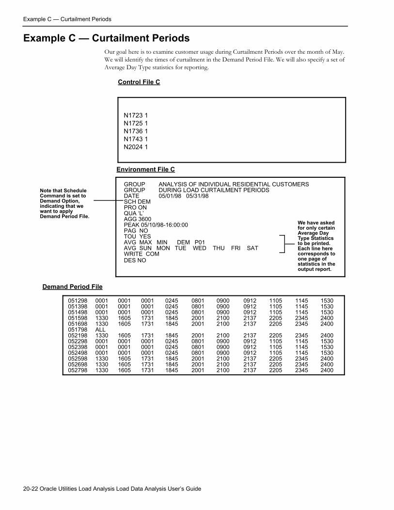
Example C — Curtailment Periods
Example C — Curtailment PeriodsOur goal here is to examine customer usage during Curtailment Periods over the month of May. We will identify the times of curtailment in the Demand Period File. We will also specify a set of Average Day Type statistics for reporting.
N1723 1N1725 1N1736 1N1743 1N2024 1
Control File C
GROUP ANALYSIS OF INDIVIDUAL RESIDENTIAL CUSTOMERSGROUP DURING LOAD CURTAILMENT PERIODSDATE 05/01/98 05/31/98SCH DEMPRO ONQUA ‘L’AGG 3600PEAK 05/10/98-16:00:00PAG NOTOU YESAVG MAX MIN DEM P01AVG SUN MON TUE WED THU FRI SATWRITE COMDES NO
Environment File C
Note that ScheduleCommand is set toDemand Option,indicating that wewant to applyDemand Period File.
We have asked for only certainAverage Day Type Statisticsto be printed.Each line herecorresponds toone page ofstatistics in theoutput report.
Demand Period File
051298051398051498051598051698051798052198052298052398052498052598052698052798
00010001000113301330ALL1330000100010001133013301330
00010001000116051605
1605000100010001160516051605
00010001000117311731
1731000100010001173117311731
02450245024518451845
1845024502450245184518451845
08010801080120012001
2001080108010801200120012001
09000900090021002100
2100090009000900210021002100
09120912091221372137
2137091209120912213721372137
11051105110522052205
2205110511051105220522052205
11451145114523452345
2345114511451145234523452345
15301530153024002400
2400153015301530240024002400
20-22 Oracle Utilities Load Analysis Load Data Analysis User’s Guide
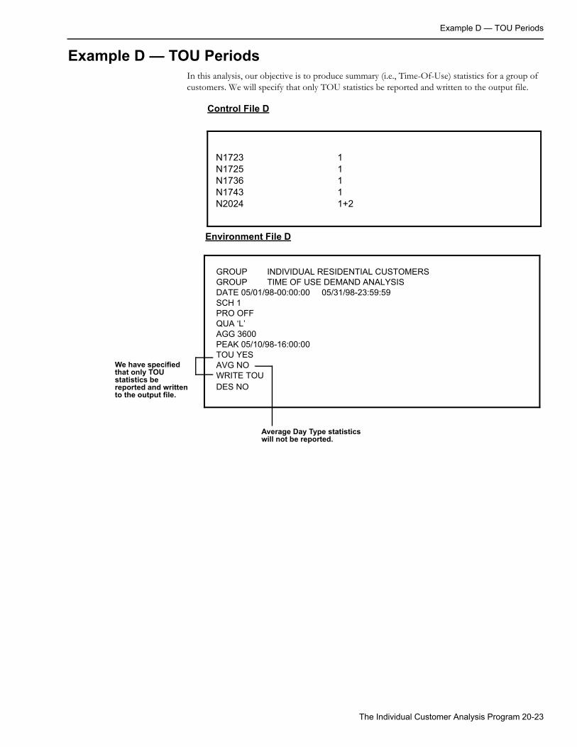
Example D — TOU Periods
Example D — TOU PeriodsIn this analysis, our objective is to produce summary (i.e., Time-Of-Use) statistics for a group of customers. We will specify that only TOU statistics be reported and written to the output file.
N1723 1N1725 1N1736 1N1743 1N2024 1+2
Control File D
GROUP INDIVIDUAL RESIDENTIAL CUSTOMERSGROUP TIME OF USE DEMAND ANALYSISDATE 05/01/98-00:00:00 05/31/98-23:59:59SCH 1PRO OFFQUA ‘L’AGG 3600PEAK 05/10/98-16:00:00TOU YESAVG NOWRITE TOUDES NO
Environment File D
We have specifiedthat only TOUstatistics bereported and writtento the output file.
Average Day Type statisticswill not be reported.
The Individual Customer Analysis Program 20-23
Individual Customer Analysis Statistics Output File Format
Individual Customer Analysis Statistics Output File FormatThe following describes the format of the two output files that can be produced by the Individual Customer Analysis Program:
• Time-Of-Use Statistics
• Average Day Statistics.
The Individual Customer Analysis Program gives you the option of creating files of customer statistics at the conclusion of a successful analysis. You can apply additional analysis or reporting routines to them. Two types of files can be created:
• Time-Of-Use Statistics
• Average Day Statistics.
The Write Command in the Environment File controls which files are created. Input “SEP” after the Write Command to produce a comma-delimited version of the report(s).
File FormatsThe file formats are shown in Table 20-3 and Table 20-4. Each output file will contain statistics for all customers in the analysis run.
In the Time-Of-Use Statistics File, each record corresponds to a single customer.
In the Average Day Statistics File, each record represents one interval in a 24-hour day.
To conserve space, the start- and stop-times in either file type refer to the earliest and latest times indicated for analysis (as opposed to recording the start- and stop-time of each individual date range included in the analysis).
20-24 Oracle Utilities Load Analysis Load Data Analysis User’s Guide
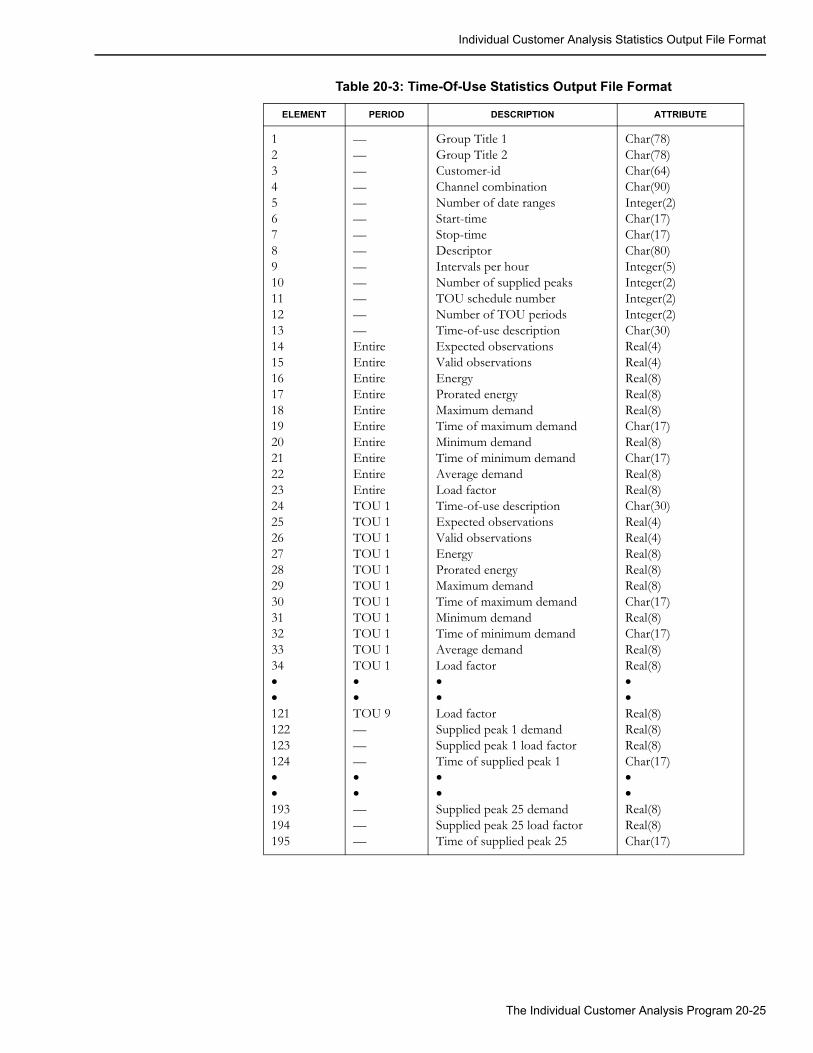
Individual Customer Analysis Statistics Output File Format
Table 20-3: Time-Of-Use Statistics Output File Format
ELEMENT PERIOD DESCRIPTION ATTRIBUTE
12345678910111213141516171819202122232425262728293031323334••121122123124••193194195
—————————————EntireEntireEntireEntireEntireEntireEntireEntireEntireEntireTOU 1TOU 1TOU 1TOU 1TOU 1TOU 1TOU 1TOU 1TOU 1TOU 1TOU 1••TOU 9———••———
Group Title 1Group Title 2Customer-idChannel combinationNumber of date rangesStart-timeStop-timeDescriptorIntervals per hourNumber of supplied peaksTOU schedule numberNumber of TOU periodsTime-of-use descriptionExpected observationsValid observationsEnergyProrated energyMaximum demandTime of maximum demandMinimum demandTime of minimum demandAverage demandLoad factorTime-of-use descriptionExpected observationsValid observationsEnergyProrated energyMaximum demandTime of maximum demandMinimum demandTime of minimum demandAverage demandLoad factor••Load factorSupplied peak 1 demandSupplied peak 1 load factorTime of supplied peak 1••Supplied peak 25 demandSupplied peak 25 load factorTime of supplied peak 25
Char(78)Char(78)Char(64)Char(90)Integer(2)Char(17)Char(17)Char(80)Integer(5)Integer(2)Integer(2)Integer(2)Char(30)Real(4)Real(4)Real(8)Real(8)Real(8)Char(17)Real(8)Char(17)Real(8)Real(8)Char(30)Real(4)Real(4)Real(8)Real(8)Real(8)Char(17)Real(8)Char(17)Real(8)Real(8)••Real(8)Real(8)Real(8)Char(17)••Real(8)Real(8)Char(17)
The Individual Customer Analysis Program 20-25

Individual Customer Analysis Statistics Output File Format
20-26 Oracle Utilities Load Analysis Load Data Analysis User’s Guide
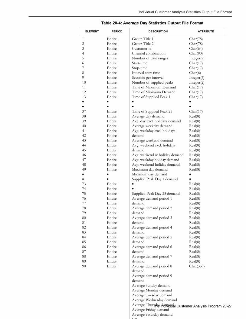
Individual Customer Analysis Statistics Output File Format
Table 20-4: Average Day Statistics Output File Format
ELEMENT PERIOD DESCRIPTION ATTRIBUTE
12345678910111213••37383940414243444546474849••737475767778798081828384858687888990
EntireEntireEntireEntireEntireEntireEntireEntireEntireEntireEntireEntireEntire••EntireEntireEntireEntireEntireEntireEntireEntireEntireEntireEntireEntireEntire••EntireEntireEntireEntireEntireEntireEntireEntireEntireEntireEntireEntireEntireEntireEntireEntireEntireEntire
Group Title 1Group Title 2Customer-idChannel combinationNumber of date rangesStart-timeStop-timeInterval start-timeSeconds per intervalNumber of supplied peaksTime of Maximum DemandTime of Minimum DemandTime of Supplied Peak 1••Time of Supplied Peak 25Average day demandAvg. day excl. holidays demandAverage weekday demandAvg. weekday excl. holidays demandAverage weekend demandAvg. weekend excl. holidays demandAvg. weekend & holiday demandAvg. weekday holiday demandAvg. weekend holiday demandMaximum day demandMinimum day demandSupplied Peak Day 1 demand••Supplied Peak Day 25 demandAverage demand period 1 demandAverage demand period 2 demandAverage demand period 3 demandAverage demand period 4 demandAverage demand period 5 demandAverage demand period 6 demandAverage demand period 7 demandAverage demand period 8 demandAverage demand period 9 demandAverage Sunday demandAverage Monday demandAverage Tuesday demand
Char(78)Char(78)Char(64)Char(90)Integer(2)Char(17)Char(17)Char(6)Integer(5)Integer(2)Char(17)Char(17)Char(17)••Char(17)Real(8)Real(8)Real(8)Real(8)Real(8)Real(8)Real(8)Real(8)Real(8)Real(8)Real(8)Real(8)••Real(8)Real(8)Real(8)Real(8)Real(8)Real(8)Real(8)Real(8)Real(8)Real(8)Real(8)Real(8)Real(8)Real(8)Real(8)Real(8)Real(8)Char(339)
The Individual Customer Analysis Program 20-27
Average Wednesday demandAverage Thursday demandAverage Friday demandAverage Saturday demandFiller

Individual Customer Analysis Statistics Output File Format
Note: Each record represents one interval in a 24-hour day. Assuming 3600-second data, the file would be structured as:
Cust-id Ch #Dates Start Stop IntervalStart SPI . . . AD ADX WD . . .
A 1 1 12019900000 123199235959 0001 3600
. . . 28 25 22 . . .
A 1 1 12019900000 123199235959 0101 3600
. . . 27 26 20 . . .
20-28 Oracle Utilities Load Analysis Load Data Analysis User’s Guide
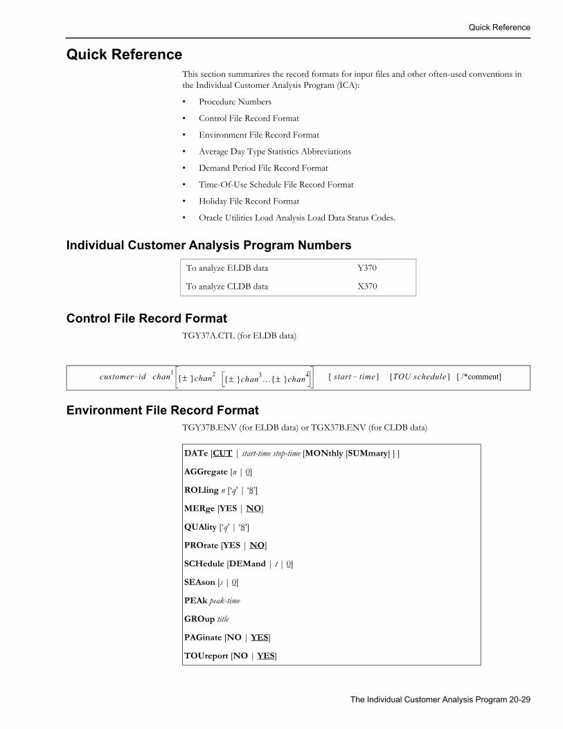
Quick Reference
Quick ReferenceThis section summarizes the record formats for input files and other often-used conventions in the Individual Customer Analysis Program (ICA):
• Procedure Numbers
• Control File Record Format
• Environment File Record Format
• Average Day Type Statistics Abbreviations
• Demand Period File Record Format
• Time-Of-Use Schedule File Record Format
• Holiday File Record Format
• Oracle Utilities Load Analysis Load Data Status Codes.
Individual Customer Analysis Program Numbers
Control File Record FormatTGY37A.CTL (for ELDB data)
Environment File Record FormatTGY37B.ENV (for ELDB data) or TGX37B.ENV (for CLDB data)
To analyze ELDB data Y370
To analyze CLDB data X370
customer id chan1– ±{ }chan2 ±{ }chan3… ±{ }chan4 [ start time ] [– TOU schedule ] [ /*comment]
DATe [CUT | start-time stop-time [MONthly [SUMmary] ] ]
AGGregate [n | 0]
ROLling n [‘q’ | ‘8’]
MERge [YES | NO]
QUAlity [‘q’ | ‘8’]
PROrate [YES | NO]
SCHedule [DEMand | t | 0]
SEAson [s | 0]
PEAk peak-time
GROup title
PAGinate [NO | YES]
TOUreport [NO | YES]
The Individual Customer Analysis Program 20-29
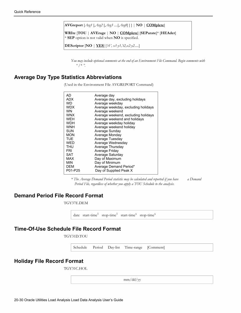
Quick Reference
You may include optional comments at the end of an Environment File Command. Begin comments with “ /* ”.
Average Day Type Statistics Abbreviations(Used in the Environment File AVGREPORT Command)
* The Average Demand Period statistic may be calculated and reported if you have a Demand Period File, regardless of whether you apply a TOU Schedule to the analysis.
Demand Period File Record FormatTGY37E.DEM
Time-Of-Use Schedule File Record FormatTGY31D.TOU
Holiday File Record FormatTGY31C.HOL
AVGreport [Avg1 [,Avg2 [,Avg3 ....[,Avg8] ] ] | NO | COMplete]
WRIte [TOU | AVErage | NO | COMplete] [SEParate]* [HEAder] * SEP option is not valid when NO is specified.
DEScriptor [NO | YES] [‘t1’, x1-y1,’t2,x2-y2.....]
AD Average dayADX Average day, excluding holidaysWD Average weekdayWDX Average weekday, excluding holidaysWN Average weekendWNX Average weekend, excluding holidaysWEH Average weekend and holidaysWDH Average weekday holidayWNH Average weekend holidaySUN Average SundayMON Average MondayTUE Average TuesdayWED Average WednesdayTHU Average ThursdayFRI Average FridaySAT Average SaturdayMAX Day of MaximumMIN Day of MinimumDEM Average Demand Period*P01-P25 Day of Supplied Peak X
date start-time1 stop-time1 start-timex stop-timex
Schedule Period Day-list Time-range [Comment]
mm/dd/yy
20-30 Oracle Utilities Load Analysis Load Data Analysis User’s Guide
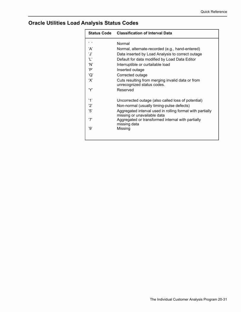
Quick Reference
Oracle Utilities Load Analysis Status Codes
Status Code Classification of Interval Data
’ ’ Normal’A’ Normal, alternate-recorded (e.g., hand-entered)’J’ Data inserted by Load Analysis to correct outage’L’ Default for data modified by Load Data Editor‘N’ Interruptible or curtailable load’P’ Inserted outage’Q’ Corrected outage‘X’ Cuts resulting from merging invalid data or from
unrecognized status codes.’Y’ Reserved
’1’ Uncorrected outage (also called loss of potential)’2’ Non-normal (usually timing-pulse defects)’5’ Aggregated interval used in rolling format with partially
missing or unavailable data’7’ Aggregated or transformed internal with partially
missing data’9’ Missing
The Individual Customer Analysis Program 20-31

Quick Reference
20-32 Oracle Utilities Load Analysis Load Data Analysis User’s Guide
Chapter 21Oracle Utilities Load Analysis Proxy Day
Selection Program (X670)
This document describes the Proxy Day Selection Program, which selects a historical day (Proxy Day) whose load shape most accurately represents a supplied day’s load shape. This selected day, in conjunction with the Cost of Service Interface, can be used to perform daily reconciliation for the estimation of aggregated suppliers’ load profiles. This program is included with the optional Analysis Bundle.
Topics included in this chapter are:
• What Does The Proxy Day Selection Program Do?
• Eligibility Testing
• Ranking of Eligible Days
• Creating the Environment File (TGX67B)
• Program Outputs
• Proxy Day Return Codes
• Proxy Day Return Code List
Oracle Utilities Load Analysis Proxy Day Selection Program (X670) 21-1
What Does The Proxy Day Selection Program Do?
What Does The Proxy Day Selection Program Do?The Proxy Day Selection Program is designed to select a historical day (Proxy Day) whose load shape most accurately represents a supplied day’s load shape. This selected day, in conjunction with the Cost of Service Interface or LPSS, can be used to perform daily reconciliation for the estimation of aggregated suppliers’ load profiles.
You can select a proxy day based on a supplied daily load shape. The program will find a daily load shape stored in a tableset that most closely matches the daily load shape you supply. The program runs against either one or two tablesets. Optional temperature data may be contained in either the same tableset as the load data or a separate tableset.
Eligibility TestingPotential proxy days are first screened for eligibility according to criteria established in the Environment File or by default. These criteria include an eligible date range, day type, holiday status, season, peak time separation, and difference of average or maximum temperature.
The optional temperature check requires a temperature cut series (Oracle Utilities Load Analysis unit of measure = 05, 13, 35, or 43) covering the same date range as the load data to be checked, and identified by a user-supplied cut series key. If only one temperature series key is provided, the same temperature series is used for both the supplied load shape day and potential proxy days; alternatively, a second temperature series may be specified for use with potential proxy days only. The temperature check calculates the average or maximum temperature of the supplied load shape day, and compares this value to the corresponding temperature data (average or maximum) for each potential proxy day. The user sets the acceptable difference in degrees between the calculated value for a potential proxy day and that for the supplied load shape day. Missing data in a day’s temperature subset will be flat-lined from the preceding non-missing value until the next non-missing temperature value is found.
The temperature cut must be of the same unit of measure (UOM) over the entire date range, and be stored in one interval tableset. If two temperature series are specified, their UOMs must be compatible. The Oracle Utilities Load Analysis tableset containing temperature data is an interval tableset, and can be the same tableset as that containing the load data or a different tableset.
21-2 Oracle Utilities Load Analysis Load Data Analysis User’s Guide
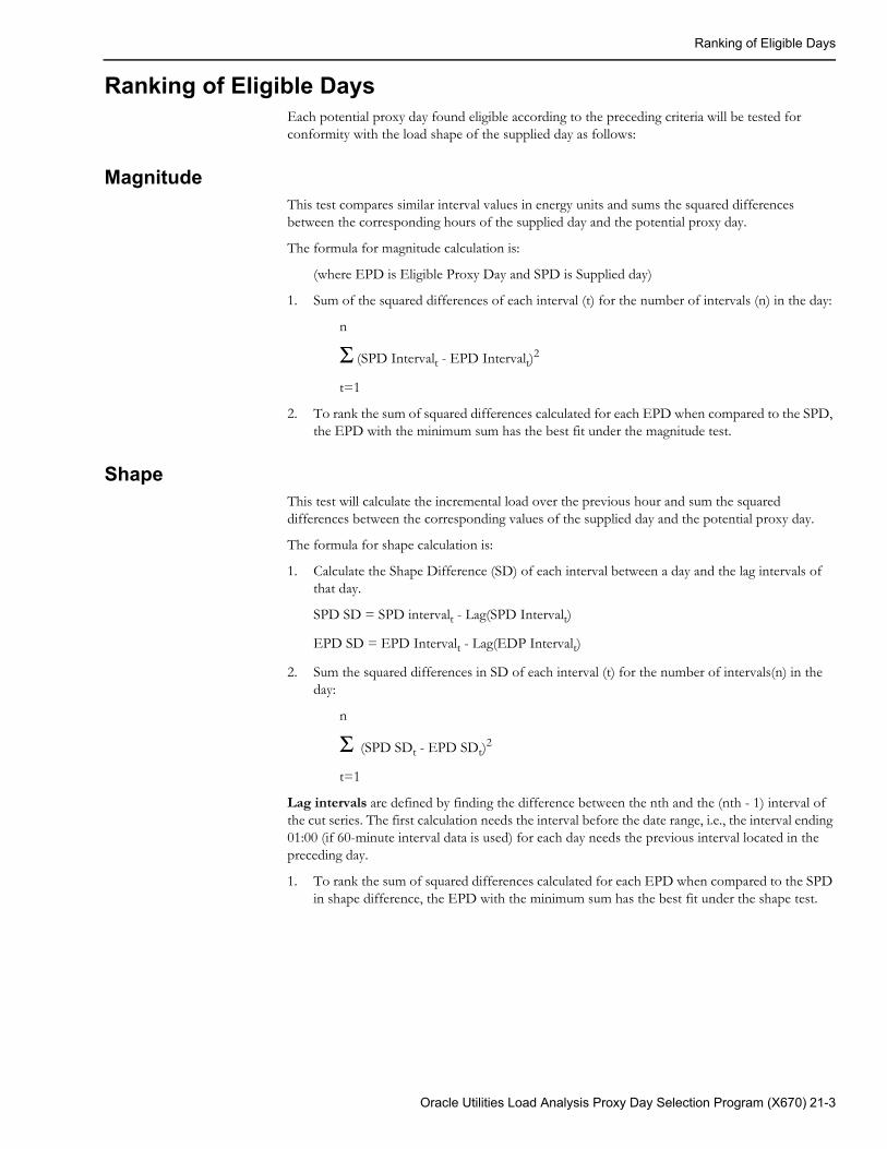
Ranking of Eligible Days
Ranking of Eligible DaysEach potential proxy day found eligible according to the preceding criteria will be tested for conformity with the load shape of the supplied day as follows:
MagnitudeThis test compares similar interval values in energy units and sums the squared differences between the corresponding hours of the supplied day and the potential proxy day.
The formula for magnitude calculation is:
(where EPD is Eligible Proxy Day and SPD is Supplied day)
1. Sum of the squared differences of each interval (t) for the number of intervals (n) in the day:
n
Σ (SPD Intervalt - EPD Intervalt)2
t=1
2. To rank the sum of squared differences calculated for each EPD when compared to the SPD, the EPD with the minimum sum has the best fit under the magnitude test.
ShapeThis test will calculate the incremental load over the previous hour and sum the squared differences between the corresponding values of the supplied day and the potential proxy day.
The formula for shape calculation is:
1. Calculate the Shape Difference (SD) of each interval between a day and the lag intervals of that day.
SPD SD = SPD intervalt - Lag(SPD Intervalt)
EPD SD = EPD Intervalt - Lag(EDP Intervalt)
2. Sum the squared differences in SD of each interval (t) for the number of intervals(n) in the day:
n
Σ (SPD SDt - EPD SDt)2
t=1
Lag intervals are defined by finding the difference between the nth and the (nth - 1) interval of the cut series. The first calculation needs the interval before the date range, i.e., the interval ending 01:00 (if 60-minute interval data is used) for each day needs the previous interval located in the preceding day.
1. To rank the sum of squared differences calculated for each EPD when compared to the SPD in shape difference, the EPD with the minimum sum has the best fit under the shape test.
Oracle Utilities Load Analysis Proxy Day Selection Program (X670) 21-3
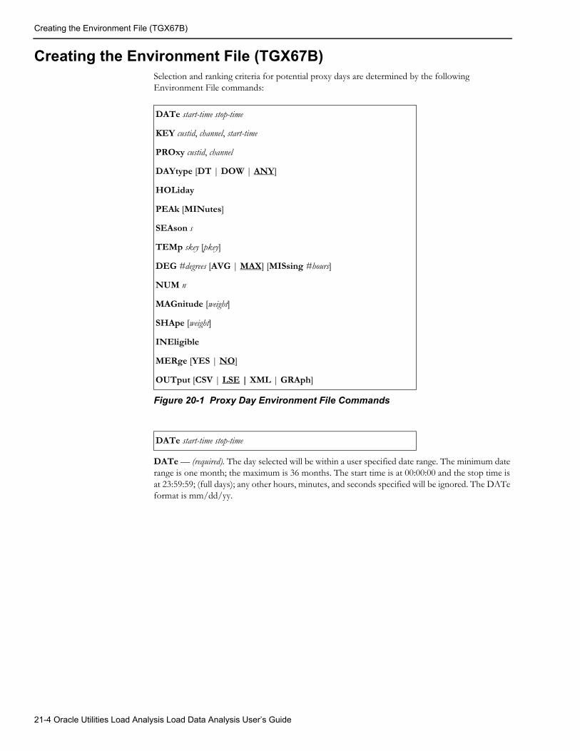
Creating the Environment File (TGX67B)
Creating the Environment File (TGX67B)Selection and ranking criteria for potential proxy days are determined by the following Environment File commands:
Figure 20-1 Proxy Day Environment File Commands
DATe — (required). The day selected will be within a user specified date range. The minimum date range is one month; the maximum is 36 months. The start time is at 00:00:00 and the stop time is at 23:59:59; (full days); any other hours, minutes, and seconds specified will be ignored. The DATe format is mm/dd/yy.
DATe start-time stop-time
KEY custid, channel, start-time
PROxy custid, channel
DAYtype [DT | DOW | ANY]
HOLiday
PEAk [MINutes]
SEAson s
TEMp skey [pkey]
DEG #degrees [AVG | MAX] [MISsing #hours]
NUM n
MAGnitude [weight]
SHApe [weight]
INEligible
MERge [YES | NO]
OUTput [CSV | LSE | XML | GRAph]
DATe start-time stop-time
21-4 Oracle Utilities Load Analysis Load Data Analysis User’s Guide
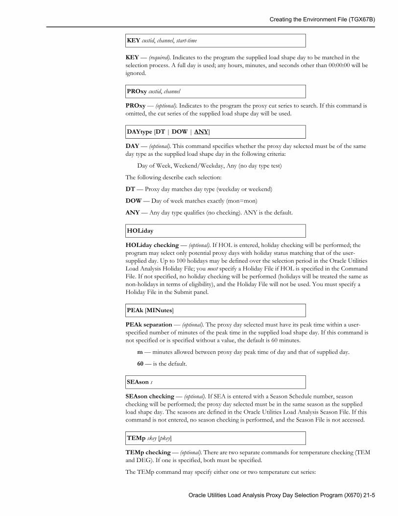
Creating the Environment File (TGX67B)
KEY — (required). Indicates to the program the supplied load shape day to be matched in the selection process. A full day is used; any hours, minutes, and seconds other than 00:00:00 will be ignored.
PROxy — (optional). Indicates to the program the proxy cut series to search. If this command is omitted, the cut series of the supplied load shape day will be used.
DAY — (optional). This command specifies whether the proxy day selected must be of the same day type as the supplied load shape day in the following criteria:
Day of Week, Weekend/Weekday, Any (no day type test)
The following describe each selection:
DT — Proxy day matches day type (weekday or weekend)
DOW — Day of week matches exactly (mon=mon)
ANY — Any day type qualifies (no checking). ANY is the default.
HOLiday checking — (optional). If HOL is entered, holiday checking will be performed; the program may select only potential proxy days with holiday status matching that of the user-supplied day. Up to 100 holidays may be defined over the selection period in the Oracle Utilities Load Analysis Holiday File; you must specify a Holiday File if HOL is specified in the Command File. If not specified, no holiday checking will be performed (holidays will be treated the same as non-holidays in terms of eligibility), and the Holiday File will not be used. You must specify a Holiday File in the Submit panel.
PEAk separation — (optional). The proxy day selected must have its peak time within a user-specified number of minutes of the peak time in the supplied load shape day. If this command is not specified or is specified without a value, the default is 60 minutes.
m — minutes allowed between proxy day peak time of day and that of supplied day.
60 — is the default.
SEAson checking — (optional). If SEA is entered with a Season Schedule number, season checking will be performed; the proxy day selected must be in the same season as the supplied load shape day. The seasons are defined in the Oracle Utilities Load Analysis Season File. If this command is not entered, no season checking is performed, and the Season File is not accessed.
TEMp checking — (optional). There are two separate commands for temperature checking (TEM and DEG). If one is specified, both must be specified.
The TEMp command may specify either one or two temperature cut series:
KEY custid, channel, start-time
PROxy custid, channel
DAYtype [DT | DOW | ANY]
HOLiday
PEAk [MINutes]
SEAson s
TEMp skey [pkey]
Oracle Utilities Load Analysis Proxy Day Selection Program (X670) 21-5
Creating the Environment File (TGX67B)
skey — skey is the key (custid/channel) of the temperature cut series providing temperatures for the supplied load shape day.
pkey — pkey is the key of the cut series providing temperatures for the potential proxy day series. If this key is omitted, the skey series will be used to find temperatures for both the supplied load shape day and the potential proxy day series.
DEG — This must be specified if the TEMp command is used.
#degrees — indicates the number of degrees by which a potential proxy day’s temperature may differ from the supplied load shape day’s. DEG must be a non-negative integer.
AVG or MAX — define which test is to be performed. If AVG is selected, the average temperatures of the potential proxy day and the supplied load shape day will be compared; if MAX is selected, their maximum temperatures will be compared. MAX is the default.
MIS #hours — is the maximum number of hours in the temperature data for any one day that may be missing (status ‘9’) and the temperature eligibility test still be performed. This must be a whole number from 0 to 23; the default is 23 if this number is not specified (i.e., only if all 24 hours of any day’s temperature data are missing will temperature testing be bypassed).
NUM Reported — (optional). n is an integer between 1 and 20. The default is 1. The program will report up to the top 20 ranked proxy days with their associated ranking values. However, no more days will be reported than meet the specified eligibility criteria.
MAGnitude weight — (optional). w is 1, 0, or a decimal fraction representing a number of tenths, such as .3 or 0.3. This command indicates to the program what weight to assign to the magnitude test described earlier.
DEG #degrees [AVG | MAX] [MISsing #hours]
NUM n
MAGnitude [weight]
21-6 Oracle Utilities Load Analysis Load Data Analysis User’s Guide
Creating the Environment File (TGX67B)
SHApe weight — (optional). w is 1, 0, or a decimal fraction representing a number of tenths. This command indicates to the program what weight to assign to the shape test described earlier.
Note: You may specify which tests are to be performed and give a weight to each test. Precision is in tenths. If a weight value is not entered, 1 is assumed. If only one test is selected and no weight is specified, the weight value for that test is defaulted to 1 and the other test is not performed. If only one test is selected and a weight is specified, the weight value for the other test is defaulted to (1 – the specified weight). If both tests are selected, the sum of the two weights must equal 1. If neither of the tests is specified in the Environment File, both tests will be performed with equal weights (.5).
INEligible — (optional). Code this command if you wish to produce the Ineligible Days Report, which lists each day within the date range that did not pass eligibility criteria, along with a message indicating the eligibility test that it failed.
MERge— An optional command. When set to “YES”, the program will merge all cuts found within the specified date range regardless of validation status. When set to “NO” (default), the program will reject invalid cuts and return an error message indicating the cuts are not merge-able.
OUTput— An optional command. Specifies the output format for the program. User can specify CSV (comma-separated output), LSE, XML, or GRAph. The use of GRAph will allow you to graphically view the selected proxy days and the supplied day.
SHApe [weight]
INEligible
MERge [YES | NO]
OUTput [CSV | LSE | XML | GRAph]
Oracle Utilities Load Analysis Proxy Day Selection Program (X670) 21-7

Program Outputs
Program OutputsThe program produces an Environment File Report and a Summary Report listing the selected proxy day(s) with ranking factor(s). In addition, it writes to output file TGX671 a single 80-character record consisting of a DATe Command defining the best-ranked proxy day selected, suitable for use by a load data extraction program such as Direct Output (X720/Y720) or Cost Of Service Data Extraction (G120). An example of the output file record:
DATE 04/23/97-00:00:00 04/23/97-23:59:59 (from X670)
21-8 Oracle Utilities Load Analysis Load Data Analysis User’s Guide
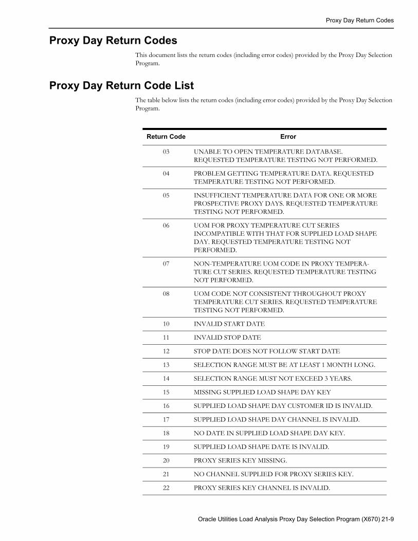
Proxy Day Return Codes
Proxy Day Return CodesThis document lists the return codes (including error codes) provided by the Proxy Day Selection Program.
Proxy Day Return Code ListThe table below lists the return codes (including error codes) provided by the Proxy Day Selection Program.
Return Code Error
03 UNABLE TO OPEN TEMPERATURE DATABASE. REQUESTED TEMPERATURE TESTING NOT PERFORMED.
04 PROBLEM GETTING TEMPERATURE DATA. REQUESTED TEMPERATURE TESTING NOT PERFORMED.
05 INSUFFICIENT TEMPERATURE DATA FOR ONE OR MORE PROSPECTIVE PROXY DAYS. REQUESTED TEMPERATURE TESTING NOT PERFORMED.
06 UOM FOR PROXY TEMPERATURE CUT SERIES INCOMPATIBLE WITH THAT FOR SUPPLIED LOAD SHAPE DAY. REQUESTED TEMPERATURE TESTING NOT PERFORMED.
07 NON-TEMPERATURE UOM CODE IN PROXY TEMPERA-TURE CUT SERIES. REQUESTED TEMPERATURE TESTING NOT PERFORMED.
08 UOM CODE NOT CONSISTENT THROUGHOUT PROXY TEMPERATURE CUT SERIES. REQUESTED TEMPERATURE TESTING NOT PERFORMED.
10 INVALID START DATE
11 INVALID STOP DATE
12 STOP DATE DOES NOT FOLLOW START DATE
13 SELECTION RANGE MUST BE AT LEAST 1 MONTH LONG.
14 SELECTION RANGE MUST NOT EXCEED 3 YEARS.
15 MISSING SUPPLIED LOAD SHAPE DAY KEY
16 SUPPLIED LOAD SHAPE DAY CUSTOMER ID IS INVALID.
17 SUPPLIED LOAD SHAPE DAY CHANNEL IS INVALID.
18 NO DATE IN SUPPLIED LOAD SHAPE DAY KEY.
19 SUPPLIED LOAD SHAPE DATE IS INVALID.
20 PROXY SERIES KEY MISSING.
21 NO CHANNEL SUPPLIED FOR PROXY SERIES KEY.
22 PROXY SERIES KEY CHANNEL IS INVALID.
Oracle Utilities Load Analysis Proxy Day Selection Program (X670) 21-9
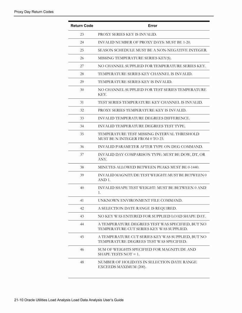
Proxy Day Return Codes
23 PROXY SERIES KEY IS INVALID.
24 INVALID NUMBER OF PROXY DAYS: MUST BE 1-20.
25 SEASON SCHEDULE MUST BE A NON-NEGATIVE INTEGER.
26 MISSING TEMPERATURE SERIES KEY(S).
27 NO CHANNEL SUPPLIED FOR TEMPERATURE SERIES KEY.
28 TEMPERATURE SERIES KEY CHANNEL IS INVALID.
29 TEMPERATURE SERIES KEY IS INVALID.
30 NO CHANNEL SUPPLIED FOR TEST SERIES TEMPERATURE KEY.
31 TEST SERIES TEMPERATURE KEY CHANNEL IS INVALID.
32 PROXY SERIES TEMPERATURE KEY IS INVALID.
33 INVALID TEMPERATURE DEGREES DIFFERENCE.
34 INVALID TEMPERATURE DEGREES TEST TYPE.
35 TEMPERATURE TEST MISSING INTERVAL THRESHOLD MUST BE N INTEGER FROM 0 TO 23.
36 INVALID PARAMETER AFTER TYPE ON DEG COMMAND.
37 INVALID DAY COMPARISON TYPE: MUST BE DOW, DT, OR ANY.
38 MINUTES ALLOWED BETWEEN PEAKS MUST BE 0-1440.
39 INVALID MAGNITUDE TEST WEIGHT: MUST BE BETWEEN 0 AND 1.
40 INVALID SHAPE TEST WEIGHT: MUST BE BETWEEN 0 AND 1.
41 UNKNOWN ENVIRONMENT FILE COMMAND.
42 A SELECTION DATE RANGE IS REQUIRED.
43 NO KEY WAS ENTERED FOR SUPPLIED LOAD SHAPE DAY.
44 A TEMPERATURE DEGREES TEST WAS SPECIFIED, BUT NO TEMPERATURE CUT SERIES KEY WAS SUPPLIED.
45 A TEMPERATURE CUT SERIES KEY WAS SUPPLIED, BUT NO TEMPERATURE DEGREES TEST WAS SPECIFIED.
46 SUM OF WEIGHTS SPECIFIED FOR MAGNITUDE AND SHAPE TESTS NOT = 1.
48 NUMBER OF HOLIDAYS IN SELECTION DATE RANGE EXCEEDS MAXIMUM (200).
Return Code Error
21-10 Oracle Utilities Load Analysis Load Data Analysis User’s Guide
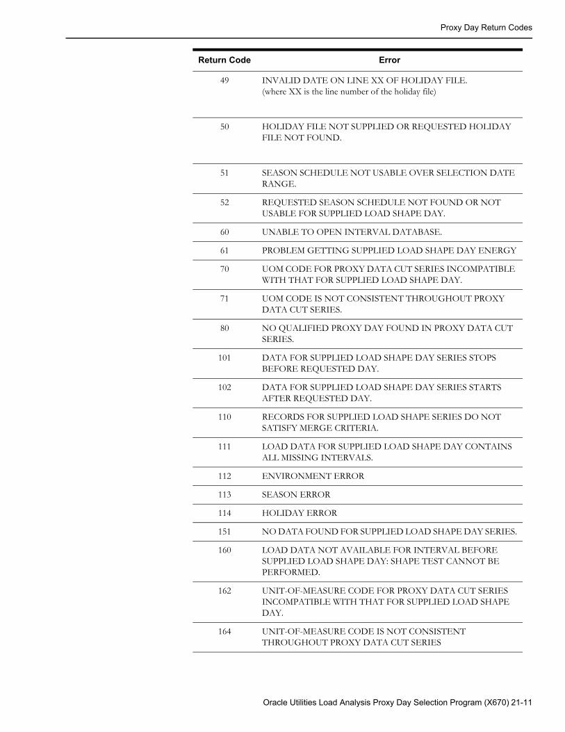
Proxy Day Return Codes
49 INVALID DATE ON LINE XX OF HOLIDAY FILE.(where XX is the line number of the holiday file)
50 HOLIDAY FILE NOT SUPPLIED OR REQUESTED HOLIDAY FILE NOT FOUND.
51 SEASON SCHEDULE NOT USABLE OVER SELECTION DATE RANGE.
52 REQUESTED SEASON SCHEDULE NOT FOUND OR NOT USABLE FOR SUPPLIED LOAD SHAPE DAY.
60 UNABLE TO OPEN INTERVAL DATABASE.
61 PROBLEM GETTING SUPPLIED LOAD SHAPE DAY ENERGY
70 UOM CODE FOR PROXY DATA CUT SERIES INCOMPATIBLE WITH THAT FOR SUPPLIED LOAD SHAPE DAY.
71 UOM CODE IS NOT CONSISTENT THROUGHOUT PROXY DATA CUT SERIES.
80 NO QUALIFIED PROXY DAY FOUND IN PROXY DATA CUT SERIES.
101 DATA FOR SUPPLIED LOAD SHAPE DAY SERIES STOPS BEFORE REQUESTED DAY.
102 DATA FOR SUPPLIED LOAD SHAPE DAY SERIES STARTS AFTER REQUESTED DAY.
110 RECORDS FOR SUPPLIED LOAD SHAPE SERIES DO NOT SATISFY MERGE CRITERIA.
111 LOAD DATA FOR SUPPLIED LOAD SHAPE DAY CONTAINS ALL MISSING INTERVALS.
112 ENVIRONMENT ERROR
113 SEASON ERROR
114 HOLIDAY ERROR
151 NO DATA FOUND FOR SUPPLIED LOAD SHAPE DAY SERIES.
160 LOAD DATA NOT AVAILABLE FOR INTERVAL BEFORE SUPPLIED LOAD SHAPE DAY: SHAPE TEST CANNOT BE PERFORMED.
162 UNIT-OF-MEASURE CODE FOR PROXY DATA CUT SERIES INCOMPATIBLE WITH THAT FOR SUPPLIED LOAD SHAPE DAY.
164 UNIT-OF-MEASURE CODE IS NOT CONSISTENT THROUGHOUT PROXY DATA CUT SERIES
Return Code Error
Oracle Utilities Load Analysis Proxy Day Selection Program (X670) 21-11
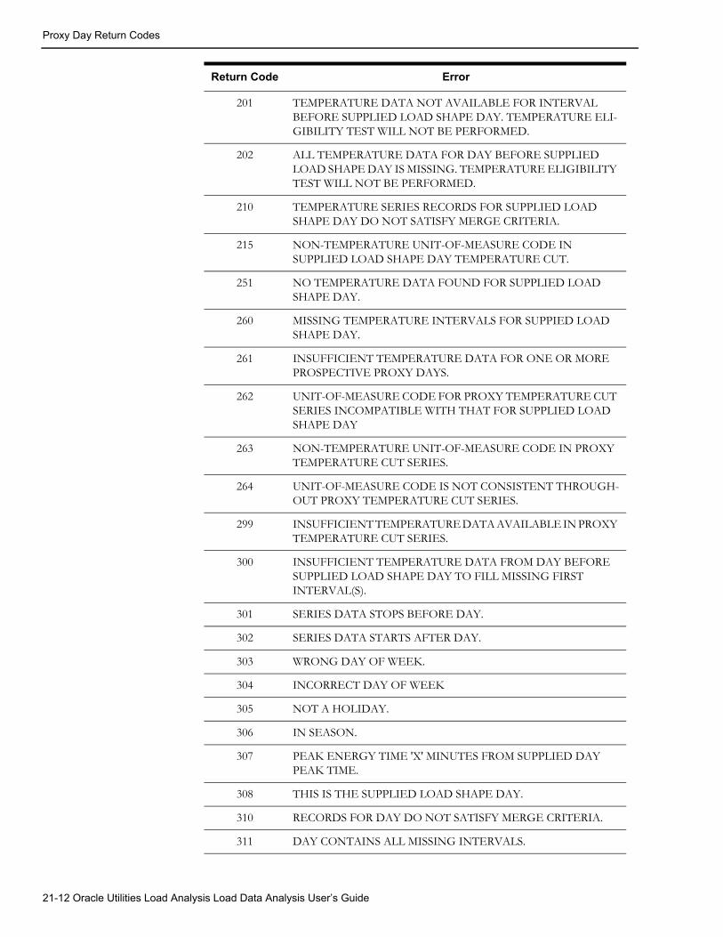
Proxy Day Return Codes
201 TEMPERATURE DATA NOT AVAILABLE FOR INTERVAL BEFORE SUPPLIED LOAD SHAPE DAY. TEMPERATURE ELI-GIBILITY TEST WILL NOT BE PERFORMED.
202 ALL TEMPERATURE DATA FOR DAY BEFORE SUPPLIED LOAD SHAPE DAY IS MISSING. TEMPERATURE ELIGIBILITY TEST WILL NOT BE PERFORMED.
210 TEMPERATURE SERIES RECORDS FOR SUPPLIED LOAD SHAPE DAY DO NOT SATISFY MERGE CRITERIA.
215 NON-TEMPERATURE UNIT-OF-MEASURE CODE IN SUPPLIED LOAD SHAPE DAY TEMPERATURE CUT.
251 NO TEMPERATURE DATA FOUND FOR SUPPLIED LOAD SHAPE DAY.
260 MISSING TEMPERATURE INTERVALS FOR SUPPIED LOAD SHAPE DAY.
261 INSUFFICIENT TEMPERATURE DATA FOR ONE OR MORE PROSPECTIVE PROXY DAYS.
262 UNIT-OF-MEASURE CODE FOR PROXY TEMPERATURE CUT SERIES INCOMPATIBLE WITH THAT FOR SUPPLIED LOAD SHAPE DAY
263 NON-TEMPERATURE UNIT-OF-MEASURE CODE IN PROXY TEMPERATURE CUT SERIES.
264 UNIT-OF-MEASURE CODE IS NOT CONSISTENT THROUGH-OUT PROXY TEMPERATURE CUT SERIES.
299 INSUFFICIENT TEMPERATURE DATA AVAILABLE IN PROXY TEMPERATURE CUT SERIES.
300 INSUFFICIENT TEMPERATURE DATA FROM DAY BEFORE SUPPLIED LOAD SHAPE DAY TO FILL MISSING FIRST INTERVAL(S).
301 SERIES DATA STOPS BEFORE DAY.
302 SERIES DATA STARTS AFTER DAY.
303 WRONG DAY OF WEEK.
304 INCORRECT DAY OF WEEK
305 NOT A HOLIDAY.
306 IN SEASON.
307 PEAK ENERGY TIME 'X' MINUTES FROM SUPPLIED DAY PEAK TIME.
308 THIS IS THE SUPPLIED LOAD SHAPE DAY.
310 RECORDS FOR DAY DO NOT SATISFY MERGE CRITERIA.
311 DAY CONTAINS ALL MISSING INTERVALS.
Return Code Error
21-12 Oracle Utilities Load Analysis Load Data Analysis User’s Guide
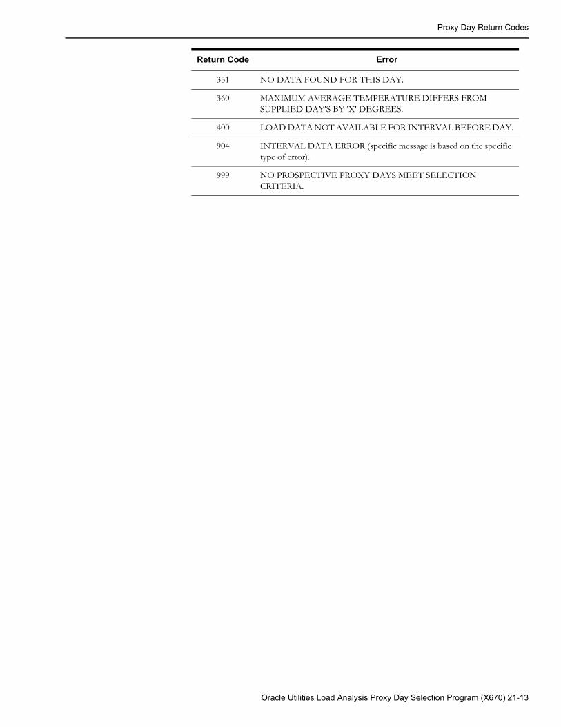
Proxy Day Return Codes
351 NO DATA FOUND FOR THIS DAY.
360 MAXIMUM AVERAGE TEMPERATURE DIFFERS FROM SUPPLIED DAY'S BY 'X' DEGREES.
400 LOAD DATA NOT AVAILABLE FOR INTERVAL BEFORE DAY.
904 INTERVAL DATA ERROR (specific message is based on the specific type of error).
999 NO PROSPECTIVE PROXY DAYS MEET SELECTION CRITERIA.
Return Code Error
Oracle Utilities Load Analysis Proxy Day Selection Program (X670) 21-13

Proxy Day Return Codes
21-14 Oracle Utilities Load Analysis Load Data Analysis User’s Guide
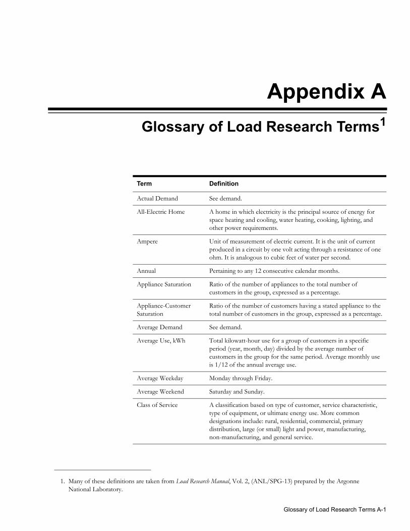
Appendix AGlossary of Load Research Terms1
1. Many of these definitions are taken from Load Research Manual, Vol. 2, (ANL/SPG-13) prepared by the Argonne National Laboratory.
Term Definition
Actual Demand See demand.
All-Electric Home A home in which electricity is the principal source of energy for space heating and cooling, water heating, cooking, lighting, and other power requirements.
Ampere Unit of measurement of electric current. It is the unit of current produced in a circuit by one volt acting through a resistance of one ohm. It is analogous to cubic feet of water per second.
Annual Pertaining to any 12 consecutive calendar months.
Appliance Saturation Ratio of the number of appliances to the total number of customers in the group, expressed as a percentage.
Appliance-Customer Saturation
Ratio of the number of customers having a stated appliance to the total number of customers in the group, expressed as a percentage.
Average Demand See demand.
Average Use, kWh Total kilowatt-hour use for a group of customers in a specific period (year, month, day) divided by the average number of customers in the group for the same period. Average monthly use is 1/12 of the annual average use.
Average Weekday Monday through Friday.
Average Weekend Saturday and Sunday.
Class of Service A classification based on type of customer, service characteristic, type of equipment, or ultimate energy use. More common designations include: rural, residential, commercial, primary distribution, large (or small) light and power, manufacturing, non-manufacturing, and general service.
Glossary of Load Research Terms A-1
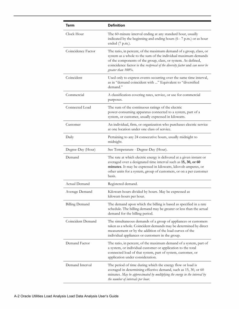
Clock Hour The 60-minute interval ending at any standard hour, usually indicated by the beginning and ending hours (6 - 7 p.m.) or as hour ended (7 p.m.).
Coincidence Factor The ratio, in percent, of the maximum demand of a group, class, or system as a whole to the sum of the individual maximum demands of the components of the group, class, or system. As defined, coincidence factor is the reciprocal of the diversity factor and can never be greater than 100%.
Coincident Used only to express events occurring over the same time interval, as in “demand coincident with ...” Equivalent to “diversified demand.”
Commercial A classification covering rates, service, or use for commercial purposes.
Connected Load The sum of the continuous ratings of the electric power-consuming apparatus connected to a system, part of a system, or customer, usually expressed in kilowatts.
Customer An individual, firm, or organization who purchases electric service at one location under one class of service.
Daily Pertaining to any 24 consecutive hours, usually midnight to midnight.
Degree-Day (Hour) See Temperature - Degree-Day (Hour).
Demand The rate at which electric energy is delivered at a given instant or averaged over a designated time interval such as 15, 30, or 60 minutes. It may be expressed in kilowatts, kilovolt-amperes, or other units for a system, group of customers, or on a per customer basis.
Actual Demand Registered demand.
Average Demand Kilowatt-hours divided by hours. May be expressed as kilowatt-hours per hour.
Billing Demand The demand upon which the billing is based as specified in a rate schedule. The billing demand may be greater or less than the actual demand for the billing period.
Coincident Demand The simultaneous demands of a group of appliances or customers taken as a whole. Coincident demands may be determined by direct measurement or by the addition of the load curves of the individual appliances or customers in the group.
Demand Factor The ratio, in percent, of the maximum demand of a system, part of a system, or individual customer or application to the total connected load of that system, part of system, customer, or application under consideration.
Demand Interval The period of time during which the energy flow or load is averaged in determining effective demand, such as 15, 30, or 60 minutes. May be approximated by multiplying the energy in the interval by the number of intervals per hour.
Term Definition
A-2 Oracle Utilities Load Analysis Load Data Analysis User’s Guide
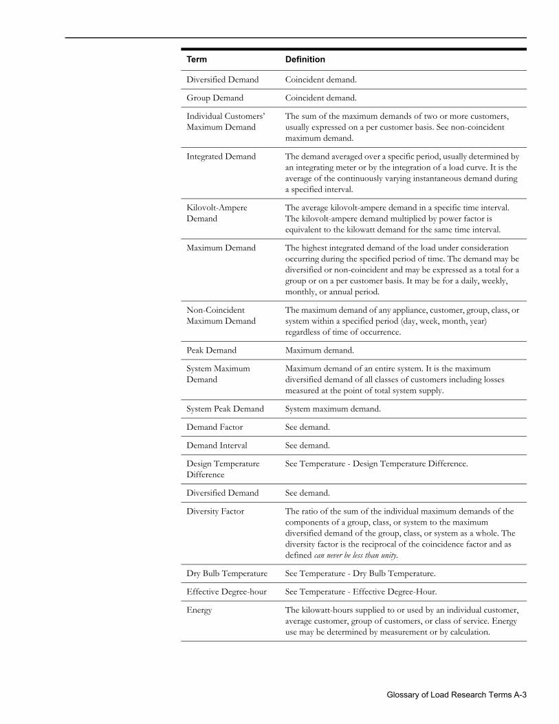
Diversified Demand Coincident demand.
Group Demand Coincident demand.
Individual Customers’ Maximum Demand
The sum of the maximum demands of two or more customers, usually expressed on a per customer basis. See non-coincident maximum demand.
Integrated Demand The demand averaged over a specific period, usually determined by an integrating meter or by the integration of a load curve. It is the average of the continuously varying instantaneous demand during a specified interval.
Kilovolt-Ampere Demand
The average kilovolt-ampere demand in a specific time interval. The kilovolt-ampere demand multiplied by power factor is equivalent to the kilowatt demand for the same time interval.
Maximum Demand The highest integrated demand of the load under consideration occurring during the specified period of time. The demand may be diversified or non-coincident and may be expressed as a total for a group or on a per customer basis. It may be for a daily, weekly, monthly, or annual period.
Non-Coincident Maximum Demand
The maximum demand of any appliance, customer, group, class, or system within a specified period (day, week, month, year) regardless of time of occurrence.
Peak Demand Maximum demand.
System Maximum Demand
Maximum demand of an entire system. It is the maximum diversified demand of all classes of customers including losses measured at the point of total system supply.
System Peak Demand System maximum demand.
Demand Factor See demand.
Demand Interval See demand.
Design Temperature Difference
See Temperature - Design Temperature Difference.
Diversified Demand See demand.
Diversity Factor The ratio of the sum of the individual maximum demands of the components of a group, class, or system to the maximum diversified demand of the group, class, or system as a whole. The diversity factor is the reciprocal of the coincidence factor and as defined can never be less than unity.
Dry Bulb Temperature See Temperature - Dry Bulb Temperature.
Effective Degree-hour See Temperature - Effective Degree-Hour.
Energy The kilowatt-hours supplied to or used by an individual customer, average customer, group of customers, or class of service. Energy use may be determined by measurement or by calculation.
Term Definition
Glossary of Load Research Terms A-3
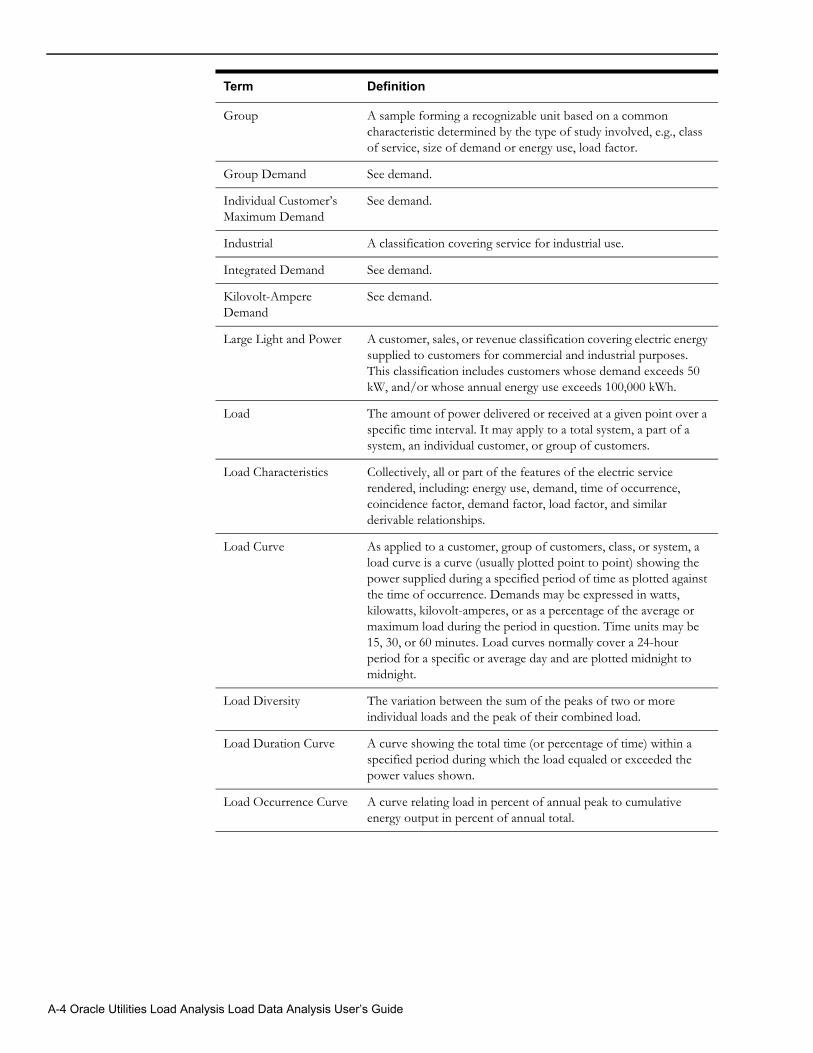
Group A sample forming a recognizable unit based on a common characteristic determined by the type of study involved, e.g., class of service, size of demand or energy use, load factor.
Group Demand See demand.
Individual Customer’s Maximum Demand
See demand.
Industrial A classification covering service for industrial use.
Integrated Demand See demand.
Kilovolt-Ampere Demand
See demand.
Large Light and Power A customer, sales, or revenue classification covering electric energy supplied to customers for commercial and industrial purposes. This classification includes customers whose demand exceeds 50 kW, and/or whose annual energy use exceeds 100,000 kWh.
Load The amount of power delivered or received at a given point over a specific time interval. It may apply to a total system, a part of a system, an individual customer, or group of customers.
Load Characteristics Collectively, all or part of the features of the electric service rendered, including: energy use, demand, time of occurrence, coincidence factor, demand factor, load factor, and similar derivable relationships.
Load Curve As applied to a customer, group of customers, class, or system, a load curve is a curve (usually plotted point to point) showing the power supplied during a specified period of time as plotted against the time of occurrence. Demands may be expressed in watts, kilowatts, kilovolt-amperes, or as a percentage of the average or maximum load during the period in question. Time units may be 15, 30, or 60 minutes. Load curves normally cover a 24-hour period for a specific or average day and are plotted midnight to midnight.
Load Diversity The variation between the sum of the peaks of two or more individual loads and the peak of their combined load.
Load Duration Curve A curve showing the total time (or percentage of time) within a specified period during which the load equaled or exceeded the power values shown.
Load Occurrence Curve A curve relating load in percent of annual peak to cumulative energy output in percent of annual total.
Term Definition
A-4 Oracle Utilities Load Analysis Load Data Analysis User’s Guide
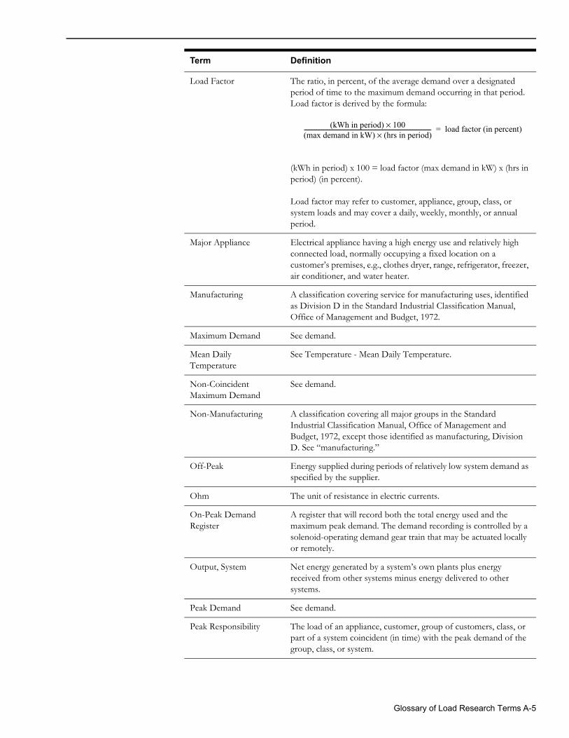
Load Factor The ratio, in percent, of the average demand over a designated period of time to the maximum demand occurring in that period. Load factor is derived by the formula:
(kWh in period) x 100 = load factor (max demand in kW) x (hrs in period) (in percent).
Load factor may refer to customer, appliance, group, class, or system loads and may cover a daily, weekly, monthly, or annual period.
Major Appliance Electrical appliance having a high energy use and relatively high connected load, normally occupying a fixed location on a customer’s premises, e.g., clothes dryer, range, refrigerator, freezer, air conditioner, and water heater.
Manufacturing A classification covering service for manufacturing uses, identified as Division D in the Standard Industrial Classification Manual, Office of Management and Budget, 1972.
Maximum Demand See demand.
Mean Daily Temperature
See Temperature - Mean Daily Temperature.
Non-Coincident Maximum Demand
See demand.
Non-Manufacturing A classification covering all major groups in the Standard Industrial Classification Manual, Office of Management and Budget, 1972, except those identified as manufacturing, Division D. See “manufacturing.”
Off-Peak Energy supplied during periods of relatively low system demand as specified by the supplier.
Ohm The unit of resistance in electric currents.
On-Peak Demand Register
A register that will record both the total energy used and the maximum peak demand. The demand recording is controlled by a solenoid-operating demand gear train that may be actuated locally or remotely.
Output, System Net energy generated by a system’s own plants plus energy received from other systems minus energy delivered to other systems.
Peak Demand See demand.
Peak Responsibility The load of an appliance, customer, group of customers, class, or part of a system coincident (in time) with the peak demand of the group, class, or system.
Term Definition
(kWh in period) 100×(max demand in kW) (hrs in period)×------------------------------------------------------------------------------------------- load factor (in percent)=
Glossary of Load Research Terms A-5
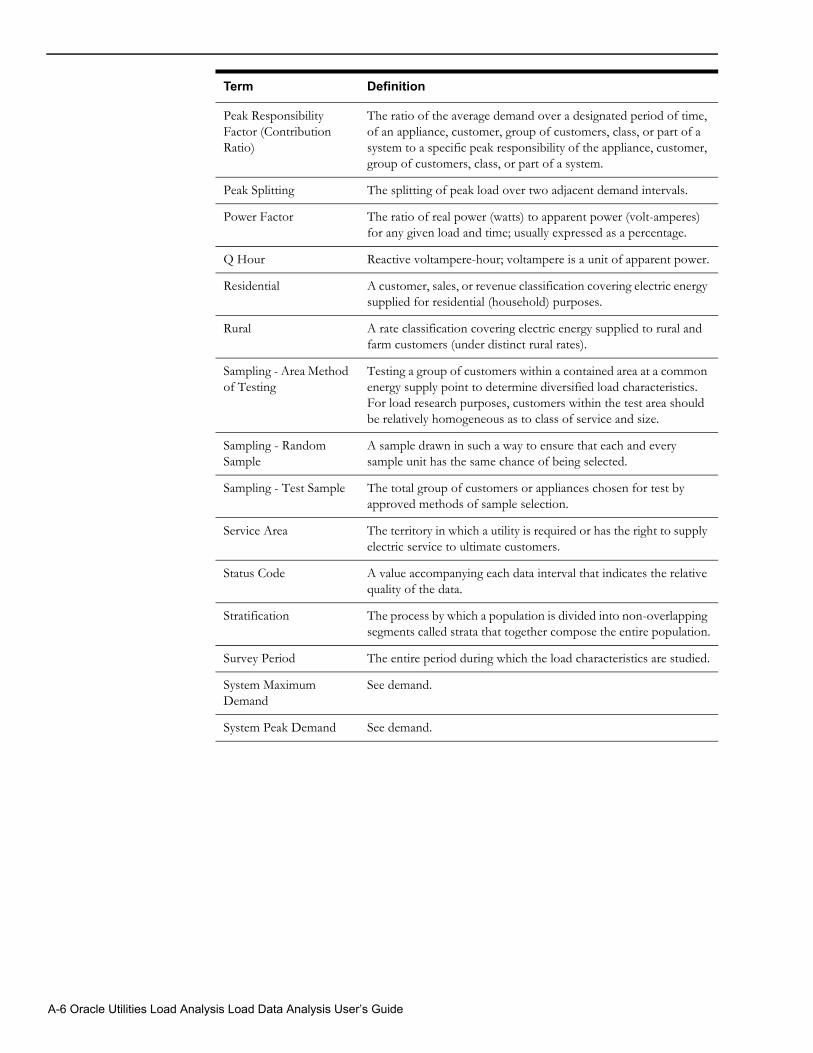
Peak Responsibility Factor (Contribution Ratio)
The ratio of the average demand over a designated period of time, of an appliance, customer, group of customers, class, or part of a system to a specific peak responsibility of the appliance, customer, group of customers, class, or part of a system.
Peak Splitting The splitting of peak load over two adjacent demand intervals.
Power Factor The ratio of real power (watts) to apparent power (volt-amperes) for any given load and time; usually expressed as a percentage.
Q Hour Reactive voltampere-hour; voltampere is a unit of apparent power.
Residential A customer, sales, or revenue classification covering electric energy supplied for residential (household) purposes.
Rural A rate classification covering electric energy supplied to rural and farm customers (under distinct rural rates).
Sampling - Area Method of Testing
Testing a group of customers within a contained area at a common energy supply point to determine diversified load characteristics. For load research purposes, customers within the test area should be relatively homogeneous as to class of service and size.
Sampling - Random Sample
A sample drawn in such a way to ensure that each and every sample unit has the same chance of being selected.
Sampling - Test Sample The total group of customers or appliances chosen for test by approved methods of sample selection.
Service Area The territory in which a utility is required or has the right to supply electric service to ultimate customers.
Status Code A value accompanying each data interval that indicates the relative quality of the data.
Stratification The process by which a population is divided into non-overlapping segments called strata that together compose the entire population.
Survey Period The entire period during which the load characteristics are studied.
System Maximum Demand
See demand.
System Peak Demand See demand.
Term Definition
A-6 Oracle Utilities Load Analysis Load Data Analysis User’s Guide
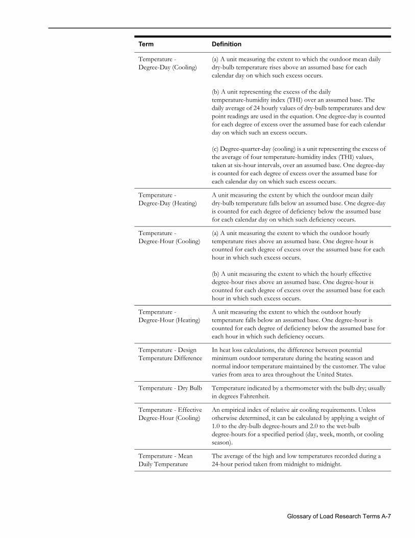
Temperature - Degree-Day (Cooling)
(a) A unit measuring the extent to which the outdoor mean daily dry-bulb temperature rises above an assumed base for each calendar day on which such excess occurs.
(b) A unit representing the excess of the daily temperature-humidity index (THI) over an assumed base. The daily average of 24 hourly values of dry-bulb temperatures and dew point readings are used in the equation. One degree-day is counted for each degree of excess over the assumed base for each calendar day on which such an excess occurs.
(c) Degree-quarter-day (cooling) is a unit representing the excess of the average of four temperature-humidity index (THI) values, taken at six-hour intervals, over an assumed base. One degree-day is counted for each degree of excess over the assumed base for each calendar day on which such excess occurs.
Temperature - Degree-Day (Heating)
A unit measuring the extent by which the outdoor mean daily dry-bulb temperature falls below an assumed base. One degree-day is counted for each degree of deficiency below the assumed base for each calendar day on which such deficiency occurs.
Temperature - Degree-Hour (Cooling)
(a) A unit measuring the extent to which the outdoor hourly temperature rises above an assumed base. One degree-hour is counted for each degree of excess over the assumed base for each hour in which such excess occurs.
(b) A unit measuring the extent to which the hourly effective degree-hour rises above an assumed base. One degree-hour is counted for each degree of excess over the assumed base for each hour in which such excess occurs.
Temperature - Degree-Hour (Heating)
A unit measuring the extent to which the outdoor hourly temperature falls below an assumed base. One degree-hour is counted for each degree of deficiency below the assumed base for each hour in which such deficiency occurs.
Temperature - Design Temperature Difference
In heat loss calculations, the difference between potential minimum outdoor temperature during the heating season and normal indoor temperature maintained by the customer. The value varies from area to area throughout the United States.
Temperature - Dry Bulb Temperature indicated by a thermometer with the bulb dry; usually in degrees Fahrenheit.
Temperature - Effective Degree-Hour (Cooling)
An empirical index of relative air cooling requirements. Unless otherwise determined, it can be calculated by applying a weight of 1.0 to the dry-bulb degree-hours and 2.0 to the wet-bulb degree-hours for a specified period (day, week, month, or cooling season).
Temperature - Mean Daily Temperature
The average of the high and low temperatures recorded during a 24-hour period taken from midnight to midnight.
Term Definition
Glossary of Load Research Terms A-7
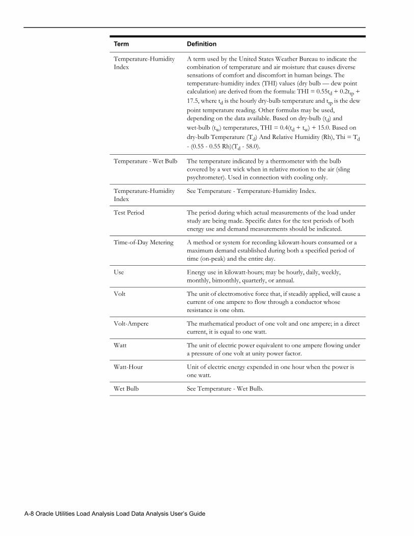
Temperature-Humidity Index
A term used by the United States Weather Bureau to indicate the combination of temperature and air moisture that causes diverse sensations of comfort and discomfort in human beings. The temperature-humidity index (THI) values (dry bulb — dew point calculation) are derived from the formula: THI = 0.55td + 0.2ttp + 17.5, where td is the hourly dry-bulb temperature and ttp is the dew point temperature reading. Other formulas may be used, depending on the data available. Based on dry-bulb (td) and wet-bulb (tw) temperatures, THI = 0.4(td + tw) + 15.0. Based on dry-bulb Temperature (Td) And Relative Humidity (Rh), Thi = Td - (0.55 - 0.55 Rh)(Td - 58.0).
Temperature - Wet Bulb The temperature indicated by a thermometer with the bulb covered by a wet wick when in relative motion to the air (sling psychrometer). Used in connection with cooling only.
Temperature-Humidity Index
See Temperature - Temperature-Humidity Index.
Test Period The period during which actual measurements of the load under study are being made. Specific dates for the test periods of both energy use and demand measurements should be indicated.
Time-of-Day Metering A method or system for recording kilowatt-hours consumed or a maximum demand established during both a specified period of time (on-peak) and the entire day.
Use Energy use in kilowatt-hours; may be hourly, daily, weekly, monthly, bimonthly, quarterly, or annual.
Volt The unit of electromotive force that, if steadily applied, will cause a current of one ampere to flow through a conductor whose resistance is one ohm.
Volt-Ampere The mathematical product of one volt and one ampere; in a direct current, it is equal to one watt.
Watt The unit of electric power equivalent to one ampere flowing under a pressure of one volt at unity power factor.
Watt-Hour Unit of electric energy expended in one hour when the power is one watt.
Wet Bulb See Temperature - Wet Bulb.
Term Definition
A-8 Oracle Utilities Load Analysis Load Data Analysis User’s Guide
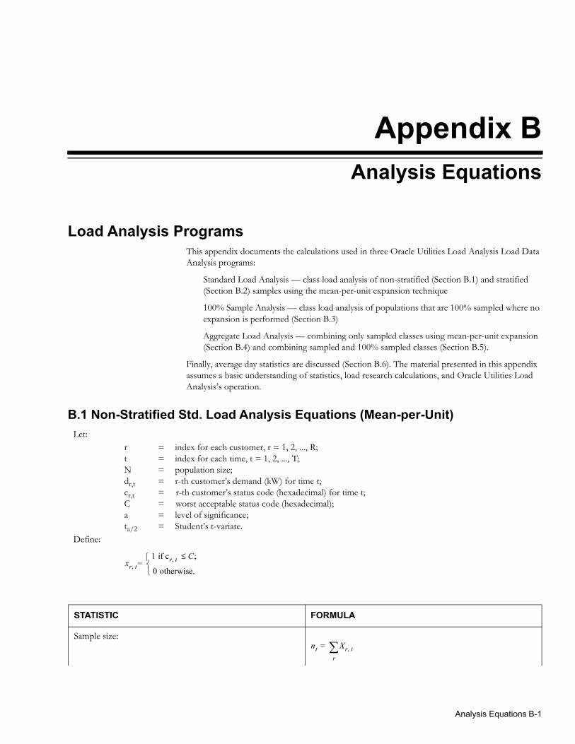
Appendix BAnalysis Equations
Load Analysis ProgramsThis appendix documents the calculations used in three Oracle Utilities Load Analysis Load Data Analysis programs:
Standard Load Analysis — class load analysis of non-stratified (Section B.1) and stratified (Section B.2) samples using the mean-per-unit expansion technique
100% Sample Analysis — class load analysis of populations that are 100% sampled where no expansion is performed (Section B.3)
Aggregate Load Analysis — combining only sampled classes using mean-per-unit expansion (Section B.4) and combining sampled and 100% sampled classes (Section B.5).
Finally, average day statistics are discussed (Section B.6). The material presented in this appendix assumes a basic understanding of statistics, load research calculations, and Oracle Utilities Load Analysis’s operation.
B.1 Non-Stratified Std. Load Analysis Equations (Mean-per-Unit) Let:
rtNdr,tcr,tCata/2
========
index for each customer, r = 1, 2, ..., R; index for each time, t = 1, 2, ..., T;population size;r-th customer’s demand (kW) for time t;r-th customer’s status code (hexadecimal) for time t;worst acceptable status code (hexadecimal);level of significance;Student’s t-variate.
Define:
xr t,1 if cr t , C;≤
0 otherwise.
=
STATISTIC FORMULA
Sample size: nt Xr t,
r=
Analysis Equations B-1
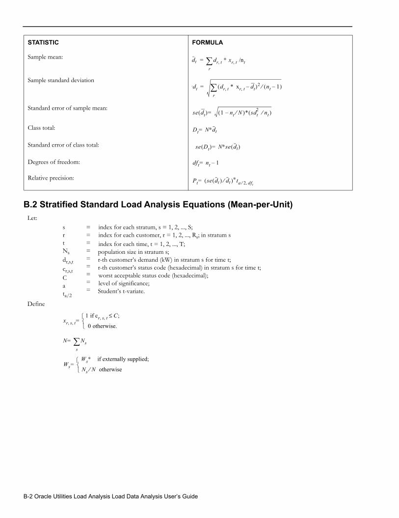
B.2 Stratified Standard Load Analysis Equations (Mean-per-Unit)
Sample mean:
Sample standard deviation
Standard error of sample mean:
Class total:
Standard error of class total:
Degrees of freedom:
Relative precision:
Let:
srtNs
dr,s,t
cr,s,t
Cata/2
=========
index for each stratum, s = 1, 2, ..., S;index for each customer, r = 1, 2, ..., Rs; in stratum sindex for each time, t = 1, 2, ..., T;population size in stratum s;r-th customer’s demand (kW) in stratum s for time t;r-th customer’s status code (hexadecimal) in stratum s for time t;worst acceptable status code (hexadecimal);level of significance;Student’s t-variate.
Define
STATISTIC FORMULA
dt dr t, ∗ xr t, /ntr=
sdt dr t, * xr t, dt–( )2 nt 1–( )⁄r=
se dt( ) 1( nt N )⁄– * sdt2 nt )⁄(=
Dt N∗dt=
se Dt( ) N∗se dt( )=
dft nt 1–=
Pt se dt ) dt⁄ )∗ta 2 dft,⁄((=
xr s t, ,1 if cr s t, , C;≤
0 otherwise.
=
N Nss=
WsWs∗ if externally supplied;
Ns N otherwise⁄
=
B-2 Oracle Utilities Load Analysis Load Data Analysis User’s Guide
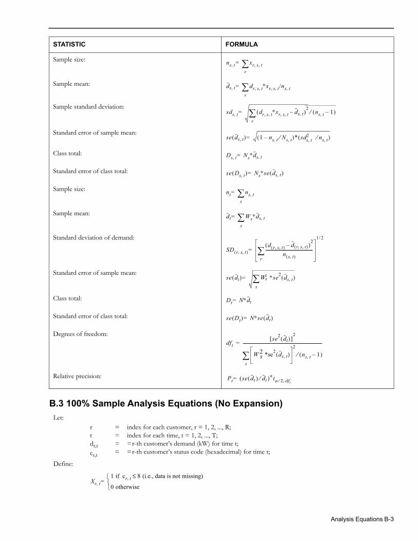
B.3 100% Sample Analysis Equations (No Expansion)
STATISTIC FORMULA
Sample size:
Sample mean:
Sample standard deviation:
Standard error of sample mean:
Class total:
Standard error of class total:
Sample size:
Sample mean:
Standard deviation of demand:
Standard error of sample mean:
Class total:
Standard error of class total:
Degrees of freedom:
Relative precision:
Let:rtdr,t
cr,t
====
index for each customer, r = 1, 2, ..., R;index for each time, t = 1, 2, ..., T;=r-th customer’s demand (kW) for time t;=r-th customer’s status code (hexadecimal) for time t;
Define:
ns t, xr s t, ,r=
ds t, dr s t, , ∗xr s t, , /ns t,r=
sds t, dr s t, , ∗xr s t, , ds t,–( )2
r ns t, 1–( )⁄=
se ds t,( ) 1 ns t, Ns t,⁄–( )* sd2s t, ns t,⁄( )=
Ds t, Ns∗ds t,=
se Ds t,( ) Ns∗se ds t,( )=
nt ns t,s=
dt Ws∗ds t,s=
SD r s t, ,( )d r s t, ,( ) d r s t, ,( )–( )
2
n s t,( )----------------------------------------------
r
1 2/
=
se dt( ) Ws2 ∗se2 ds t,( )s=
Dt N∗dt=
se Dt( ) N∗se dt( )=
dftse2 dt( )[ ]
2
W 2s *se2 ds t,( )
2
ns t, 1–( )⁄s-----------------------------------------------------------------------------=
Pt se dt ) dt⁄ )∗ta 2 dft,⁄((=
Xr t,1 if cr t, 8 (i.e., data is not missing)≤
0 otherwise
=
Analysis Equations B-3
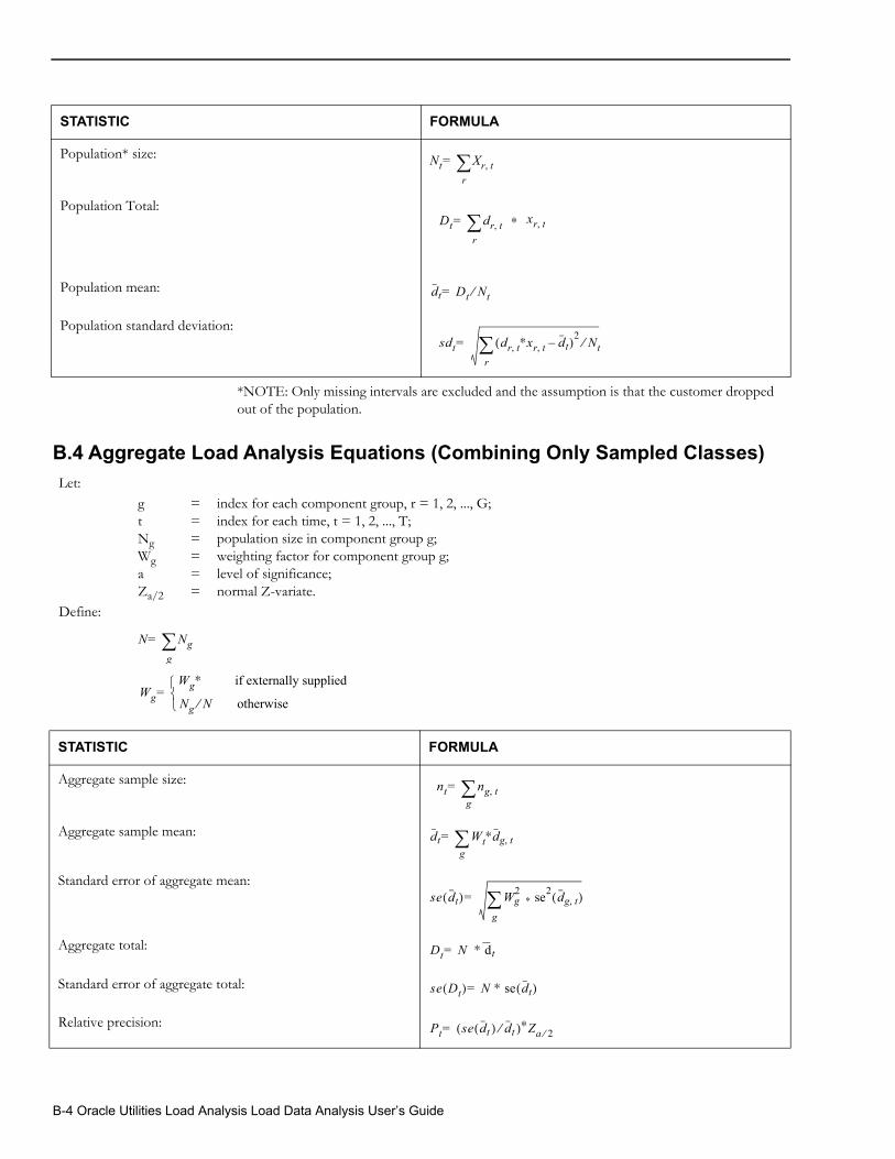
*NOTE: Only missing intervals are excluded and the assumption is that the customer dropped out of the population.
B.4 Aggregate Load Analysis Equations (Combining Only Sampled Classes)
STATISTIC FORMULA
Population* size:
Population Total:
Population mean:
Population standard deviation:
Nt Xr t,r=
Dt dr t,r=
∗
xr t,
dt Dt Nt⁄=
sdt dr t, ∗xr t, dt–( )2 Nt⁄r=
Let:gtNgWgaZa/2
======
index for each component group, r = 1, 2, ..., G;index for each time, t = 1, 2, ..., T;population size in component group g;weighting factor for component group g;level of significance;normal Z-variate.
Define:
STATISTIC FORMULA
Aggregate sample size:
Aggregate sample mean:
Standard error of aggregate mean:
Aggregate total:
Standard error of aggregate total:
Relative precision:
N Ngg=
WgWg∗ if externally supplied
Ng N otherwise⁄
=
nt ng t,g=
dt Wt∗dg t,g=
se dt( ) W2g ∗ se2 dg t,( )
g =
Dt N ∗ dt =
se Dt( ) N ∗ se dt( )=
Pt se dt(( ) dt⁄ )∗Za 2⁄=
B-4 Oracle Utilities Load Analysis Load Data Analysis User’s Guide
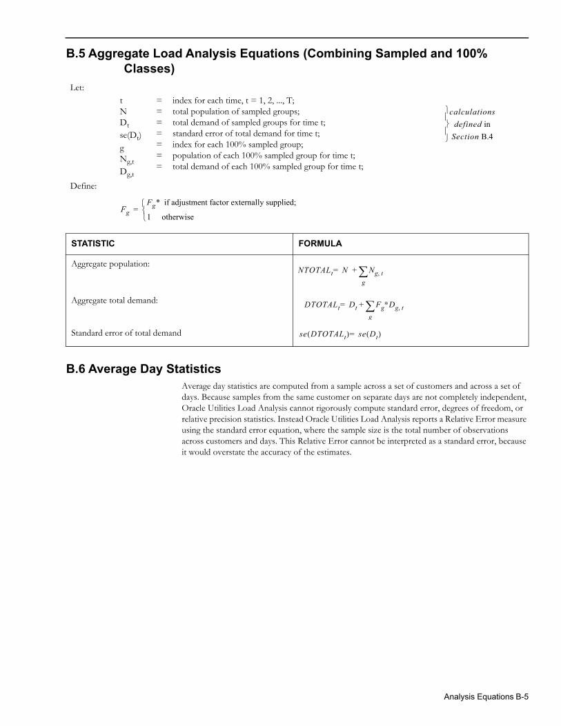
B.5 Aggregate Load Analysis Equations (Combining Sampled and 100% Classes)
B.6 Average Day StatisticsAverage day statistics are computed from a sample across a set of customers and across a set of days. Because samples from the same customer on separate days are not completely independent, Oracle Utilities Load Analysis cannot rigorously compute standard error, degrees of freedom, or relative precision statistics. Instead Oracle Utilities Load Analysis reports a Relative Error measure using the standard error equation, where the sample size is the total number of observations across customers and days. This Relative Error cannot be interpreted as a standard error, because it would overstate the accuracy of the estimates.
Let:
tNDt
se(Dt)gNg,t
Dg,t
=======
index for each time, t = 1, 2, ..., T;total population of sampled groups;total demand of sampled groups for time t;standard error of total demand for time t;index for each 100% sampled group;population of each 100% sampled group for time t;total demand of each 100% sampled group for time t;
Define:
STATISTIC FORMULA
Aggregate population:
Aggregate total demand:
Standard error of total demand
calculationsdefined inSection B.4
FgFg* if adjustment factor externally supplied;
1 otherwise
=
NTOTALt N Ng t,g+=
DTOTALt Dt Fg∗Dg t,g+=
se DTOTALt( ) se Dt( )=
Analysis Equations B-5

B-6 Oracle Utilities Load Analysis Load Data Analysis User’s Guide

Appendix CRatio Analysis Equations
This appendix documents the ratio analysis calculations used in Oracle Utilities Load Analysis. This material assumes a basic understanding of statistics, load research calculations, and Oracle Utilities Load Analysis’s operation.
Ratio Analysis Equations C-1
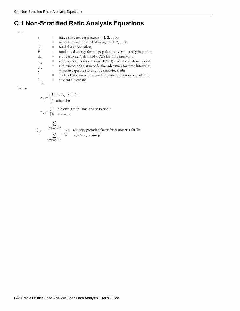
C.1 Non-Stratified Ratio Analysis Equations
C.1 Non-Stratified Ratio Analysis EquationsLet:
rtNEdr,t
er,t
cr,t
Cata/2
==========
index for each customer, r = 1, 2, ..., R;index for each interval of time, t = 1, 2, ..., T;total class population;total billed energy for the population over the analysis period;r-th customer’s demand (KW) for time interval t;r-th customer’s total energy (KWH) over the analysis period;r-th customer’s status code (hexadecimal) for time interval t;worst acceptable status code (haxadecimal);1 - level of significance used in relative precision calculation;student’s t-variate;
Define:
xr t,1 if Cr t , C=<( )
0 otherwise
=
mt p,1 if interval t is in Time-of-Use Period P0 otherwise
=
fr p = ,
τ ρ?New 3E?
τ ρ?New 3E?
mt p,xr t,
e( nergy proration factor for customer r for Timof Use period p )–
C-2 Oracle Utilities Load Analysis Load Data Analysis User’s Guide
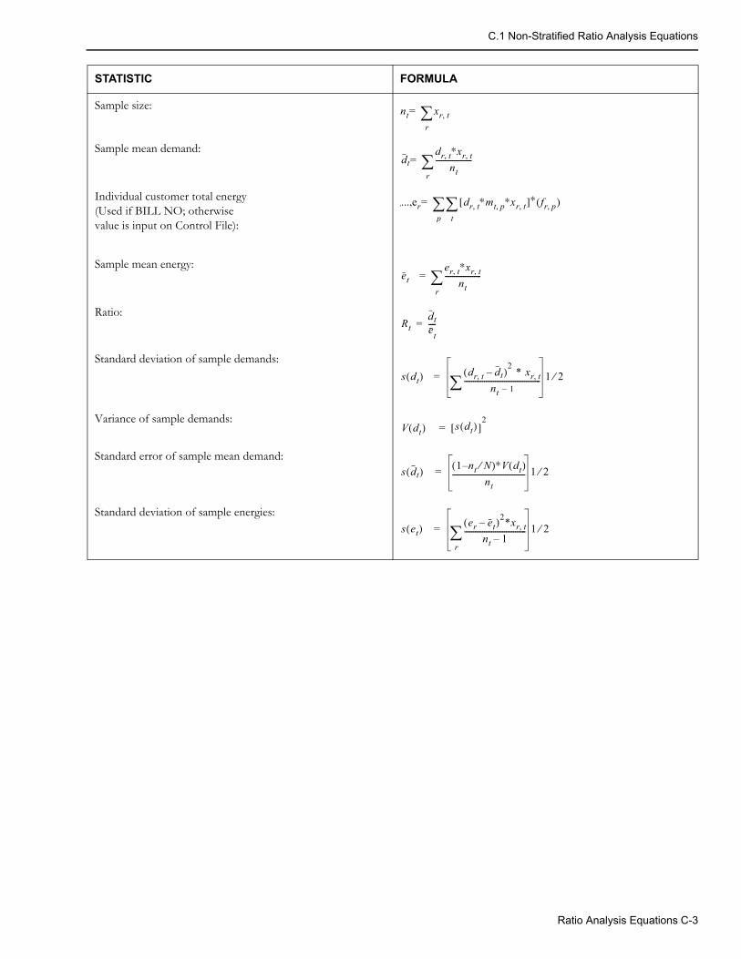
C.1 Non-Stratified Ratio Analysis Equations
STATISTIC FORMULA
Sample size:
Sample mean demand:
Individual customer total energy(Used if BILL NO; otherwisevalue is input on Control File):
Sample mean energy:
Ratio:
Standard deviation of sample demands:
Variance of sample demands:
Standard error of sample mean demand:
Standard deviation of sample energies:
nt xr t,r=
dtdr t, ∗xr t,nt
--------------------r=
,...,er dr t, ∗mt p, ∗xr t,[ ]∗ fr p,( )t
p=
eter t, ∗xr t,nt
--------------------r=
Rtdtet----=
s dt( ) dr t, dt–( )2 * xr t,
nt 1 –------------------------------------------ 1 2⁄=
V dt( ) s dt( )[ ]2
=
s dt( ) 1 nt N⁄–( )∗V dt( )nt
---------------------------------------- 1 2⁄=
s et( ) er et–( )2*xr t,nt 1–
----------------------------------r 1 2⁄=
Ratio Analysis Equations C-3
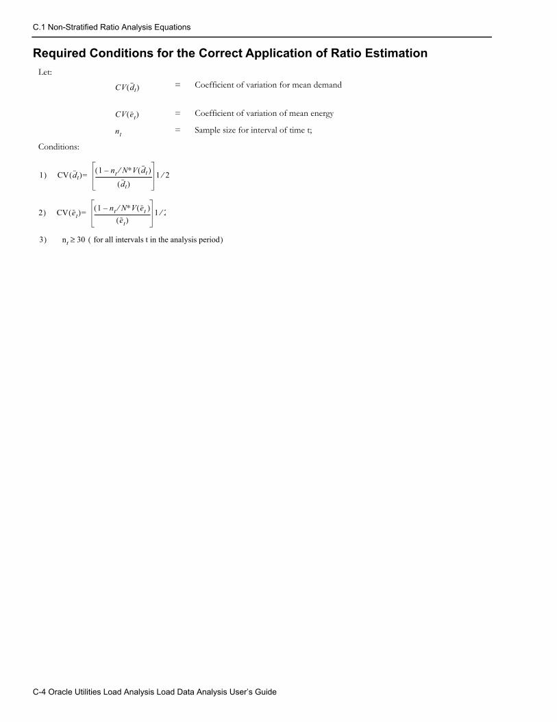
C.1 Non-Stratified Ratio Analysis Equations
Required Conditions for the Correct Application of Ratio EstimationLet:
= Coefficient of variation for mean demand
= Coefficient of variation of mean energy
= Sample size for interval of time t;
Conditions:
CV dt( )
CV et( )
nt
1( ) CV dt( ) 1 nt N∗V⁄ dt )(–(
dt( )------------------------------------------ 1 2⁄=
2) CV et( ) 1 nt N∗V et(⁄ )–(et( )
----------------------------------------- 1 2⁄=
3( ) nt 30 for all intervals t in the analysis period( )≥
C-4 Oracle Utilities Load Analysis Load Data Analysis User’s Guide

C.2 Separate (Stratified) Ratio Analysis Equations
C.2 Separate (Stratified) Ratio Analysis EquationsLet:
rStNNs
Es
dr,s,t
er,s,t
cr,s,t
Cata/2
============
index for each customer, r = 1, 2, ..., R;index for each strata within the sample, s = 1, 2, 3, ..., S;index for each interval of time, t = 1, 2, 3, ..., T;total class population;strata population;total billed energy for strata s over the analysis period;demand (KW) for the r-th customer in strata s for time interval t;total energy (KWH) for the r-th customer in strata s for time interval t;status code (hexadecimal) for the r-th customer in strata s for time interval t;worst acceptable status code (hexadecimal);1 - level of significance used in relative precision calculation;student’s t-variate;
Define:
Xr s t, ,1 if cr t < = C,
0 otherwise
=
mt p,1 if interval t is in Time-of-Use Period p0 otherwise
=
=
τ ρ?New 3E?
τ ρ?New 3E?
mt p,xr s t, ,
e( nergy proration factor for customer r for Tim
of Use period p) –
WsNs N weighting factor for strata s⁄
Ws∗ externally supplied weighting factor
=
Ratio Analysis Equations C-5
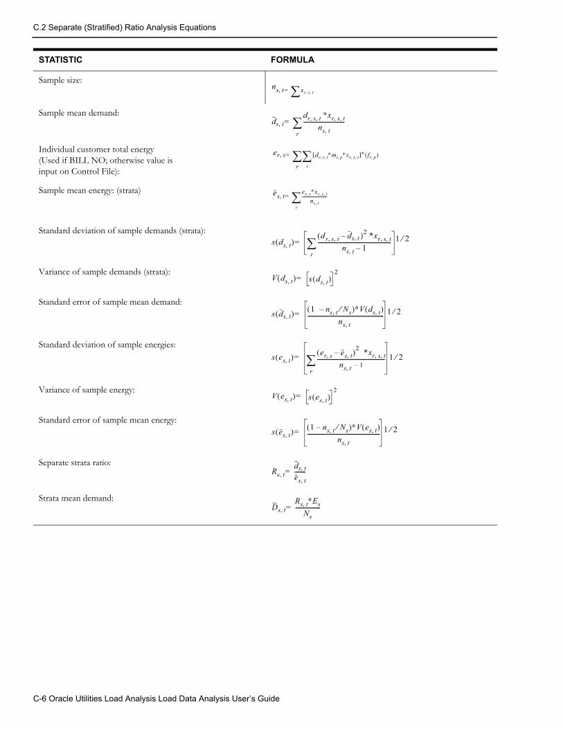
C.2 Separate (Stratified) Ratio Analysis Equations
STATISTIC FORMULA
Sample size:
Sample mean demand:
Individual customer total energy(Used if BILL NO; otherwise value is input on Control File):
Sample mean energy: (strata)
Standard deviation of sample demands (strata):
Variance of sample demands (strata):
Standard error of sample mean demand:
Standard deviation of sample energies:
Variance of sample energy:
Standard error of sample mean energy:
Separate strata ratio:
Strata mean demand:
ns t xr s t, ,=,
ds t,dr s t , , ∗xr s t, ,
ns t,------------------------------
r=
er s dr s t, , ∗mt p, ∗xr s t, ,[ ]∗ fr p,( )
t
p=,
es t er s, ∗xr s t, ,ns t,
-----------------------r=,
s ds t,( )d( r s t, , ds t, )– 2 *xr s t, ,
ns t, 1–-----------------------------------------------------
r 1 2⁄=
V ds t,( ) s ds t,( )2
=
s ds t,( ) 1 ns t, Ns⁄–( )∗V ds t,( )ns t ,
------------------------------------------------------- 1 2⁄=
s es t,( ) er s, es t,–( )2 *xr s t, ,ns t 1–,
-------------------------------------------------r 1 2⁄=
V es t,( ) s es t,( )2
=
s es t,( ) 1 ns t, Ns⁄–( )∗V es t,( )ns t,
----------------------------------------------------- 1 2⁄=
Rs t,ds t,es t,--------=
Ds t,Rs t, ∗EsNs
------------------=
C-6 Oracle Utilities Load Analysis Load Data Analysis User’s Guide
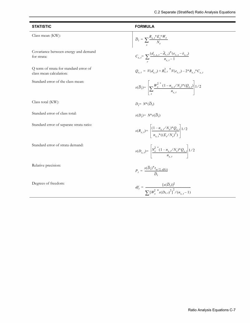
C.2 Separate (Stratified) Ratio Analysis Equations
Class mean (KW):
Covariance between energy and demandfor strata:
Q term of strata for standard error ofclass mean calculation:
Standard error of the class mean:
Class total (KW):
Standard error of class total:
Standard error of separate strata ratio:
Standard error of strata demand:
Relative precision:
Degrees of freedom:
STATISTIC FORMULA
DtRs t, ∗Es ∗Ws
Ns------------------------------
s=
Cs t,dr s t, , ds t,–( )∗ er s, es t,–( )
ns t, 1–---------------------------------------------------------------
r=
Qs t, V ds t,( ) R2s t,
∗V es t,( ) 2∗Rs t, ∗C– s t,+=
s Dt( ) Ws2 ∗ 1 ns t, Ns⁄–( )∗ Qs t,( )
ns t,----------------------------------------------------------------
s 1 2⁄=
Dt N∗ Dt( )=
s Dt( ) N∗s Dt( )=
s Rs t,( )1 ns t, Ns⁄–( )∗Qs t,ns t, ∗ Es Ns⁄( )2( )
--------------------------------------------- 1 2⁄=
s Ds t,( ) Ns2 ∗
1 ns t, Ns⁄–( )∗Qs t,ns t,
--------------------------------------------------------- 1 2⁄=
Pts Dt( )∗ta 2 df t( ),⁄
Dt--------------------------------------=
dfts Dt( )[ ]
Ws2 ∗s Ds t,( )2[ ]
2ns t, 1–( )⁄
--------------------------------------------------------------------------2
=
Ratio Analysis Equations C-7
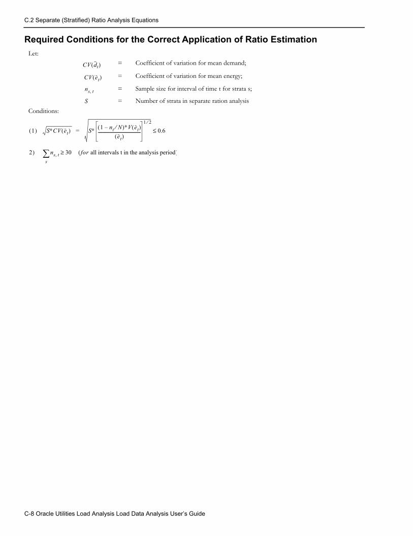
C.2 Separate (Stratified) Ratio Analysis Equations
Required Conditions for the Correct Application of Ratio EstimationLet:
= Coefficient of variation for mean demand;
= Coefficient of variation for mean energy;
= Sample size for interval of time t for strata s;
= Number of strata in separate ration analysis
Conditions:
CV dt( )
CV et( )
ns t,
S
1( ) S∗CV et( ) = S∗ 1 nt N⁄–( )∗V et( )et( )
------------------------------------------1 2⁄
0.6≤
2( ) ns t, 30 for all intervals t in the analysis period( )≥s
C-8 Oracle Utilities Load Analysis Load Data Analysis User’s Guide
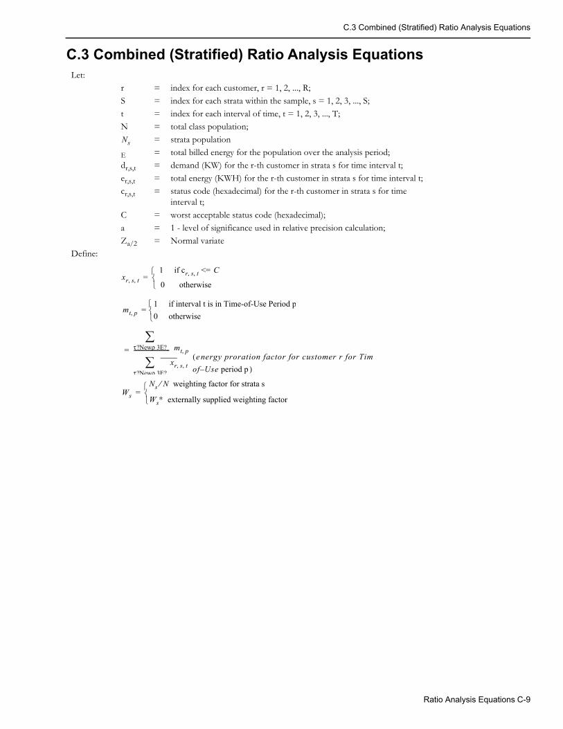
C.3 Combined (Stratified) Ratio Analysis Equations
C.3 Combined (Stratified) Ratio Analysis EquationsLet:
r = index for each customer, r = 1, 2, ..., R;
S = index for each strata within the sample, s = 1, 2, 3, ..., S;t = index for each interval of time, t = 1, 2, 3, ..., T;N = total class population;
= strata population
E = total billed energy for the population over the analysis period;dr,s,t = demand (KW) for the r-th customer in strata s for time interval t;
er,s,t = total energy (KWH) for the r-th customer in strata s for time interval t;cr,s,t = status code (hexadecimal) for the r-th customer in strata s for time
interval t;C = worst acceptable status code (hexadecimal);
a = 1 - level of significance used in relative precision calculation;Za/2 = Normal variate
Define:
Ns
xr s t, , 1 if cr s t , , <= C
0 otherwise
=
mt p,1 if interval t is in Time-of-Use Period p0 otherwise
=
τ ρ?New 3E?
τ ρ?New 3E?
--------------------------
mt p,
xr s t, ,
e( nergy proration factor for customer r for Timof Use period p )–
=
WsNs N weighting factor for strata s⁄
Ws∗ externally supplied weighting factor
=
Ratio Analysis Equations C-9
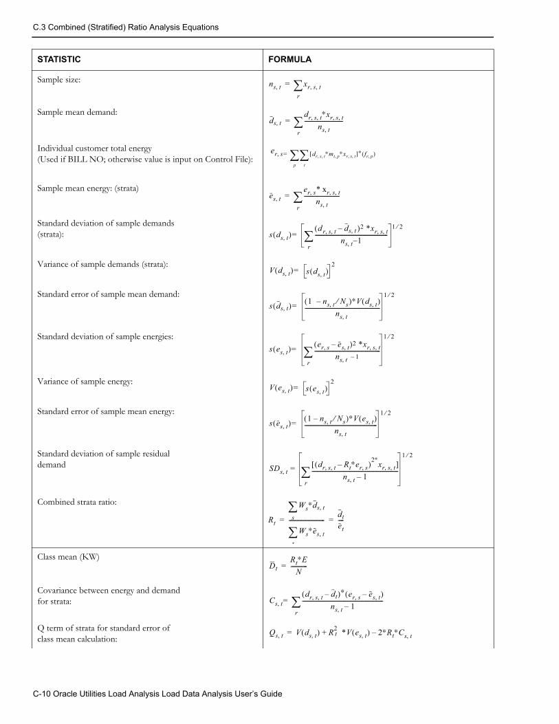
C.3 Combined (Stratified) Ratio Analysis Equations
STATISTIC FORMULA
Sample size:
Sample mean demand:
Individual customer total energy(Used if BILL NO; otherwise value is input on Control File):
Sample mean energy: (strata)
Standard deviation of sample demands(strata):
Variance of sample demands (strata):
Standard error of sample mean demand:
Standard deviation of sample energies:
Variance of sample energy:
Standard error of sample mean energy:
Standard deviation of sample residualdemand
Combined strata ratio:
Class mean (KW)
Covariance between energy and demandfor strata:
Q term of strata for standard error ofclass mean calculation:
ns t, xr s t, ,r=
ds t,dr s t, , ∗xr s t, ,
ns t,----------------------------
r=
er s dr s t, , ∗mt p, ∗xr s t, ,[ ]∗ fr p,( )
t
p=,
es t,er s, * xr s t, ,ns t,
--------------------------r=
s ds t,( )d( r s t, , ds t, )– 2 *xr s t, ,
ns t, 1–-----------------------------------------------------
r
1 2⁄=
V ds t,( ) s ds t,( )2
=
s ds t,( ) 1 ns t, Ns⁄–( )∗V ds t,( )ns t ,
-------------------------------------------------------1 2⁄
=
s es t,( ) er s, es t,–( )2 *xr s t, ,ns t 1–,
------------------------------------------------r
1 2⁄
=
V es t,( ) s es t,( )2
=
s es t,( ) 1 ns t, Ns⁄–( )∗V es t,( )ns t,
-----------------------------------------------------1 2⁄
=
SDs t,dr s t, , Rt∗er s,–( )2∗
xr s t, ,[ ]ns t, 1–
---------------------------------------------------------------r
1 2⁄
=
Rt
Ws∗ds t,s
Ws∗es t,s-------------------------- dt
et----= =
DtRt∗EN
------------=
Cs t,dr s t, , dt–( )∗ er s, es t,–( )
ns t, 1–-----------------------------------------------------------
r=
Qs t, V ds t,( ) R2t *V es t,( ) 2∗Rt∗C– s t,+=
C-10 Oracle Utilities Load Analysis Load Data Analysis User’s Guide
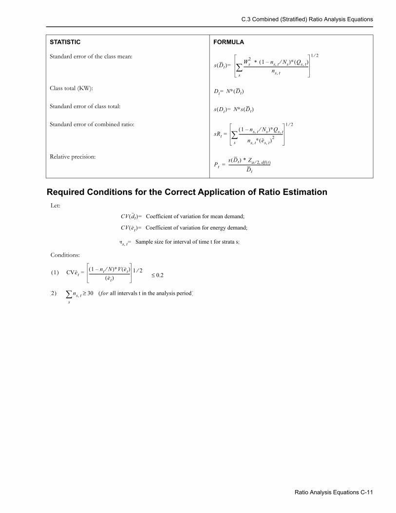
C.3 Combined (Stratified) Ratio Analysis Equations
Required Conditions for the Correct Application of Ratio Estimation
Standard error of the class mean:
Class total (KW):
Standard error of class total:
Standard error of combined ratio:
Relative precision:
Let:
Conditions:
STATISTIC FORMULA
s Dt( ) Ws2 * 1 ns t, Ns⁄–( )∗ Qs t,( )
ns t,-------------------------------------------------------------------
s
1 2⁄
=
Dt N∗ Dt( )=
s Dt( ) N∗s Dt( )=
sRt1 ns t, Ns⁄–( )∗Qs t,ns t, ∗ es t,( )2
---------------------------------------------s
1 2⁄
=
Pts Dt( ) * Za 2 df t( ),⁄
Dt-------------------------------------------=
CV dt( ) Coefficient of variation for mean demand;=
CV et( ) Coefficient of variation for energy demand;=
ns t, Sample size for interval of time t for strata s;=
1( ) CVet1 nt N⁄–( )∗V et( )
et( )------------------------------------------ 1 2⁄
0.2≤=
2( ) ns t, 30 for all intervals t in the analysis period( )≥s
Ratio Analysis Equations C-11

Average Day Statistics
Average Day StatisticsAverage day statistics are computed from a sample across a set of customers and across a set of days. Since samples from the same customer on separate days are not completely independent, Oracle Utilities Load Analysis cannot rigorously compute standard error, degrees of freedom, or relative precision statistics. Instead Oracle Utilities Load Analysis reports a Relative Error measure using the standard error equation, where the sample size is the total number of observations across customers and days. This Relative Error cannot be interpreted as a standard error, because it would overstate the accuracy of the estimates.
C-12 Oracle Utilities Load Analysis Load Data Analysis User’s Guide
Appendix DReading “Analysis Statistics Written to the
ELDB” Reports and Listings of AnalysisStatistic Names
This appendix begins with a detailed description of the “Statistics Written to the ELDB” report. This report is a very useful summary of the statistics produced and saved during an analysis run.
The remainder of the appendix documents the names assigned to analysis statistics produced by Oracle Utilities Analysis programs. It includes the entire set of names for non-stratified and stratified standard load analysis statistics, non-stratified, combined, and separate ratio statistics, 100% sample statistics, and aggregate analysis statistics. The order of the statistic listings is:
1. Non-Stratified and Stratified Standard Load Analysis (these use the same naming conventions)
2. Non-Stratified Ratio Analysis
3. Stratified Ratio Analysis (Combined and Separate)
4. 100% Sample Analysis
5. Aggregate Analysis: Sample Only Mode
6. Aggregate Analysis: 100% Mode.
All of these statistics are produced by the associated analysis run and written back to the ELDB for future analysis.
Reading “Analysis Statistics Written to the ELDB” Reports and Listings of Analysis Statistic Names D-1
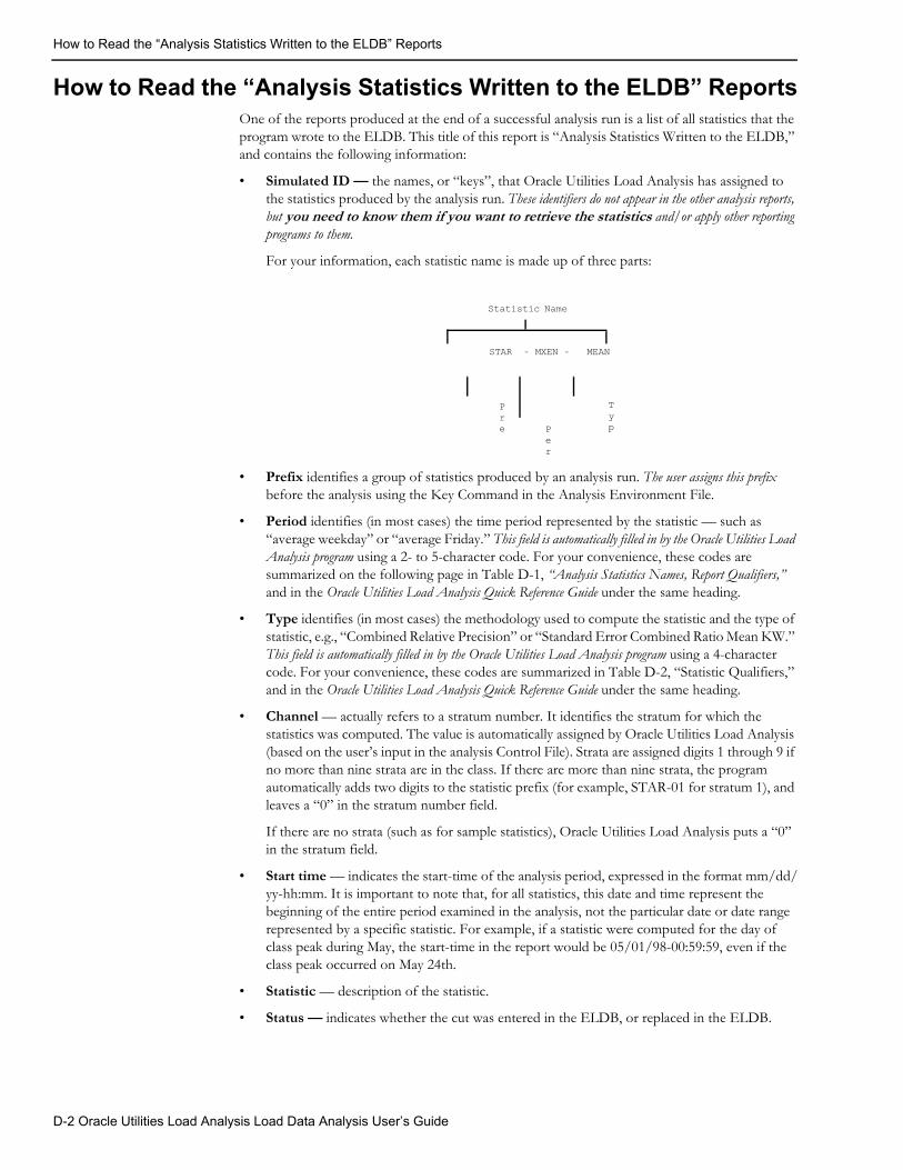
How to Read the “Analysis Statistics Written to the ELDB” Reports
How to Read the “Analysis Statistics Written to the ELDB” ReportsOne of the reports produced at the end of a successful analysis run is a list of all statistics that the program wrote to the ELDB. This title of this report is “Analysis Statistics Written to the ELDB,” and contains the following information:
• Simulated ID — the names, or “keys”, that Oracle Utilities Load Analysis has assigned to the statistics produced by the analysis run. These identifiers do not appear in the other analysis reports, but you need to know them if you want to retrieve the statistics and/or apply other reporting programs to them.
For your information, each statistic name is made up of three parts:
• Prefix identifies a group of statistics produced by an analysis run. The user assigns this prefix before the analysis using the Key Command in the Analysis Environment File.
• Period identifies (in most cases) the time period represented by the statistic — such as “average weekday” or “average Friday.” This field is automatically filled in by the Oracle Utilities Load Analysis program using a 2- to 5-character code. For your convenience, these codes are summarized on the following page in Table D-1, “Analysis Statistics Names, Report Qualifiers,” and in the Oracle Utilities Load Analysis Quick Reference Guide under the same heading.
• Type identifies (in most cases) the methodology used to compute the statistic and the type of statistic, e.g., “Combined Relative Precision” or “Standard Error Combined Ratio Mean KW.” This field is automatically filled in by the Oracle Utilities Load Analysis program using a 4-character code. For your convenience, these codes are summarized in Table D-2, “Statistic Qualifiers,” and in the Oracle Utilities Load Analysis Quick Reference Guide under the same heading.
• Channel — actually refers to a stratum number. It identifies the stratum for which the statistics was computed. The value is automatically assigned by Oracle Utilities Load Analysis (based on the user’s input in the analysis Control File). Strata are assigned digits 1 through 9 if no more than nine strata are in the class. If there are more than nine strata, the program automatically adds two digits to the statistic prefix (for example, STAR-01 for stratum 1), and leaves a “0” in the stratum number field.
If there are no strata (such as for sample statistics), Oracle Utilities Load Analysis puts a “0” in the stratum field.
• Start time — indicates the start-time of the analysis period, expressed in the format mm/dd/yy-hh:mm. It is important to note that, for all statistics, this date and time represent the beginning of the entire period examined in the analysis, not the particular date or date range represented by a specific statistic. For example, if a statistic were computed for the day of class peak during May, the start-time in the report would be 05/01/98-00:59:59, even if the class peak occurred on May 24th.
• Statistic — description of the statistic. description of the statistic.
• Status — indicates whether the cut was entered in the ELDB, or replaced in the ELDB.-
STAR - MXEN - MEAN
Statistic Name
Pre P
er
Typ
D-2 Oracle Utilities Load Analysis Load Data Analysis User’s Guide
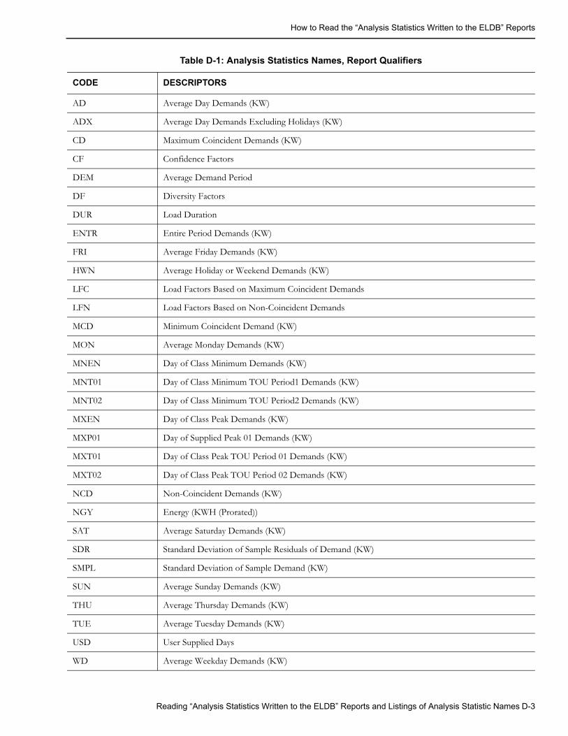
How to Read the “Analysis Statistics Written to the ELDB” Reports
Table D-1: Analysis Statistics Names, Report Qualifiers
CODE DESCRIPTORS
AD Average Day Demands (KW)
ADX Average Day Demands Excluding Holidays (KW)
CD Maximum Coincident Demands (KW)
CF Confidence Factors
DEM Average Demand Period
DF Diversity Factors
DUR Load Duration
ENTR Entire Period Demands (KW)
FRI Average Friday Demands (KW)
HWN Average Holiday or Weekend Demands (KW)
LFC Load Factors Based on Maximum Coincident Demands
LFN Load Factors Based on Non-Coincident Demands
MCD Minimum Coincident Demand (KW)
MON Average Monday Demands (KW)
MNEN Day of Class Minimum Demands (KW)
MNT01 Day of Class Minimum TOU Period1 Demands (KW)
MNT02 Day of Class Minimum TOU Period2 Demands (KW)
MXEN Day of Class Peak Demands (KW)
MXP01 Day of Supplied Peak 01 Demands (KW)
MXT01 Day of Class Peak TOU Period 01 Demands (KW)
MXT02 Day of Class Peak TOU Period 02 Demands (KW)
NCD Non-Coincident Demands (KW)
NGY Energy (KWH (Prorated))
SAT Average Saturday Demands (KW)
SDR Standard Deviation of Sample Residuals of Demand (KW)
SMPL Standard Deviation of Sample Demand (KW)
SUN Average Sunday Demands (KW)
THU Average Thursday Demands (KW)
TUE Average Tuesday Demands (KW)
USD User Supplied Days
WD Average Weekday Demands (KW)
Reading “Analysis Statistics Written to the ELDB” Reports and Listings of Analysis Statistic Names D-3
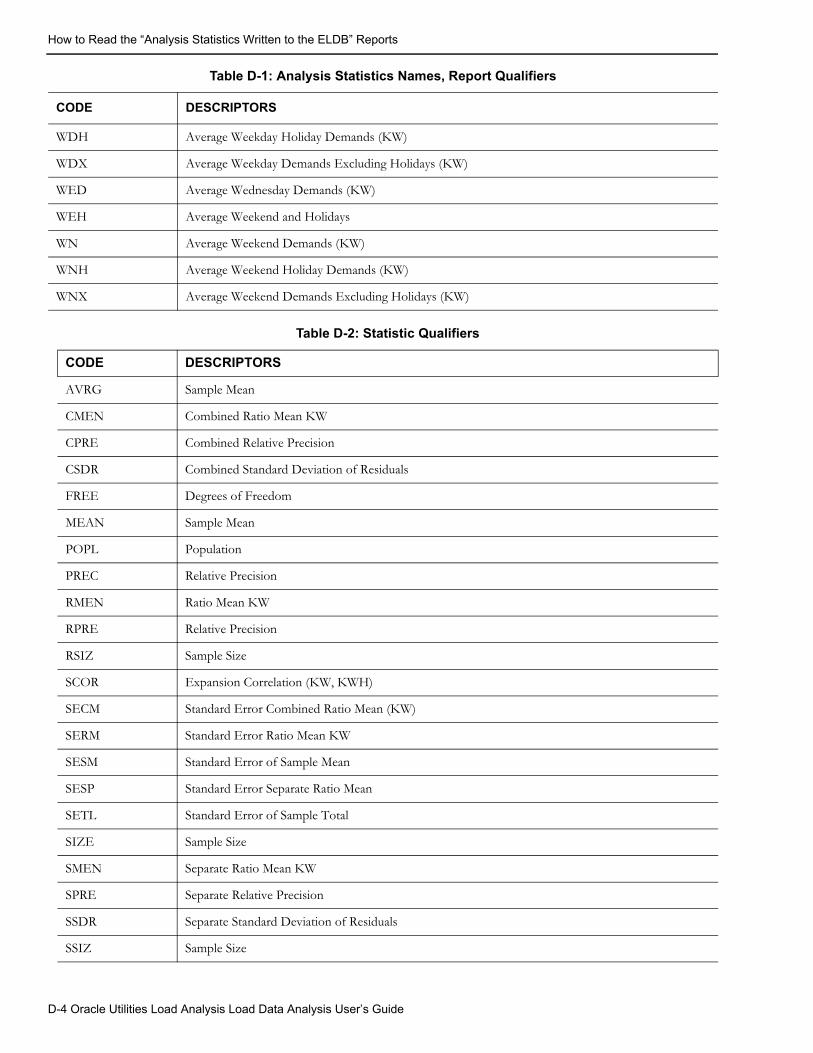
How to Read the “Analysis Statistics Written to the ELDB” Reports
WDH Average Weekday Holiday Demands (KW)
WDX Average Weekday Demands Excluding Holidays (KW)
WED Average Wednesday Demands (KW)
WEH Average Weekend and Holidays
WN Average Weekend Demands (KW)
WNH Average Weekend Holiday Demands (KW)
WNX Average Weekend Demands Excluding Holidays (KW)
Table D-1: Analysis Statistics Names, Report Qualifiers
CODE DESCRIPTORS
Table D-2: Statistic Qualifiers
CODE DESCRIPTORS
AVRG Sample Mean
CMEN Combined Ratio Mean KW
CPRE Combined Relative Precision
CSDR Combined Standard Deviation of Residuals
FREE Degrees of Freedom
MEAN Sample Mean
POPL Population
PREC Relative Precision
RMEN Ratio Mean KW
RPRE Relative Precision
RSIZ Sample Size
SCOR Expansion Correlation (KW, KWH)
SECM Standard Error Combined Ratio Mean (KW)
SERM Standard Error Ratio Mean KW
SESM Standard Error of Sample Mean
SESP Standard Error Separate Ratio Mean
SETL Standard Error of Sample Total
SIZE Sample Size
SMEN Separate Ratio Mean KW
SPRE Separate Relative Precision
SSDR Separate Standard Deviation of Residuals
SSIZ Sample Size
D-4 Oracle Utilities Load Analysis Load Data Analysis User’s Guide

How to Read the “Analysis Statistics Written to the ELDB” Reports
SSTU 10% T-Statistic
STDV Standard Deviation of Sample Demand
TOTL Total Demand
Table D-2: Statistic Qualifiers
CODE DESCRIPTORS
Reading “Analysis Statistics Written to the ELDB” Reports and Listings of Analysis Statistic Names D-5

How to Read the “Analysis Statistics Written to the ELDB” Reports
D-6 Oracle Utilities Load Analysis Load Data Analysis User’s Guide
Appendix EIndividual Customer Statistics File Formats
This appendix describes the formats and content of the Individual Customer Statistics (ICS) files that are produced by the following Oracle Utilities Analysis programs.
• Standard Load Analysis (Y310)
• Ratio Analysis (Y330)
• Domains MPU (Y350)
• Domains Ratio (Y360)
• 100% Sample Analysis (Y380).
The Individual Customer Statistics File is produced at the conclusion of a successful run of the Standard Load, Ratio, Domains MPU, Domains Ratio, and 100% Sampled Analysis programs. This file contains basic load statistics for each customer included in the analysis (one record per customer).
The content of the ICS file varies slightly from program to program. On the following pages, you will find tables that describe the binary and character formats produced by each analysis program.
Here are some additional notes about the files produced by each program:
Standard Load Analysis (Y310)Statistics are written for the entire period, each of 9 time-of-use periods, the strata peak, and 25 supplied peaks. If a preliminary analysis is performed, the time-of-use period and strata peak coincident demands are set to missing. Missing values are indicated by -9999.
Ratio Analysis (Y330)Statistics are written for the entire period, each of 9 time-of-use periods, the strata peak, 23 supplied peaks, and customer billed energy. If a preliminary analysis is performed, the time-of-use period coincident demands are set to missing. Missing values are indicated by -9999.
Domains MPU (Y350)Each record in the file corresponds to a single customer. Statistics are written for the entire period, each of 9 time-of-use periods, the strata peak, and 25 supplied peaks. If a preliminary analysis is performed, the time-of-use period coincident demands are set to missing. Missing values are indicated by -9999.
Individual Customer Statistics File Formats E-1
Domains Ratio (Y360)Each record in the file corresponds to a single customer. Statistics are written for the entire period, each of 9 time-of-use periods, the strata peak, and 25 supplied peaks. If a preliminary analysis is performed, the time-of-use period coincident demands are set to missing. Missing values are indicated by -9999.
100% Sample Analysis (Y380)Each record in the file corresponds to a single customer. Statistics are written for the entire period, each of nine time-of-use periods, and 25 supplied peaks. If a preliminary analysis is performed, time-of-use period coincident demands are set to missing. Missing values are indicated by -9999.
E-2 Oracle Utilities Load Analysis Load Data Analysis User’s Guide
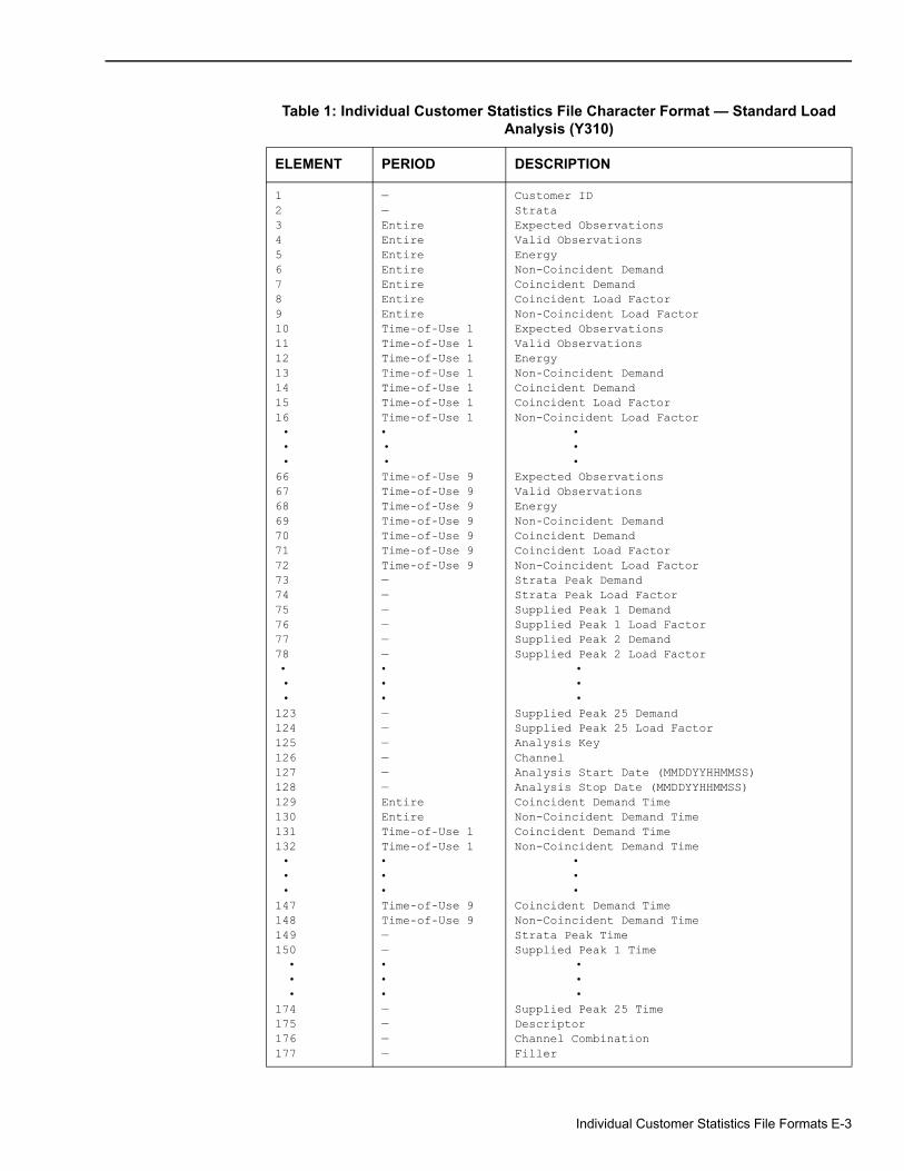
Table 1: Individual Customer Statistics File Character Format — Standard Load
Analysis (Y310)
ELEMENT PERIOD DESCRIPTION
12345678910111213141516 • • •66676869707172737475767778 • • •123124125126127128129130131132 • • •147148149150 • • •174175176177
——EntireEntireEntireEntireEntireEntireEntireTime-of-Use 1Time-of-Use 1Time-of-Use 1Time-of-Use 1Time-of-Use 1Time-of-Use 1Time-of-Use 1• • •Time-of-Use 9Time-of-Use 9Time-of-Use 9Time-of-Use 9Time-of-Use 9Time-of-Use 9Time-of-Use 9——————•••——————EntireEntireTime-of-Use 1Time-of-Use 1•••Time-of-Use 9Time-of-Use 9——•••————
Customer IDStrataExpected ObservationsValid ObservationsEnergyNon-Coincident DemandCoincident DemandCoincident Load FactorNon-Coincident Load FactorExpected ObservationsValid ObservationsEnergyNon-Coincident DemandCoincident DemandCoincident Load FactorNon-Coincident Load Factor • • •Expected ObservationsValid ObservationsEnergyNon-Coincident DemandCoincident DemandCoincident Load FactorNon-Coincident Load FactorStrata Peak DemandStrata Peak Load FactorSupplied Peak 1 DemandSupplied Peak 1 Load FactorSupplied Peak 2 DemandSupplied Peak 2 Load Factor • • •Supplied Peak 25 DemandSupplied Peak 25 Load FactorAnalysis KeyChannelAnalysis Start Date (MMDDYYHHMMSS)Analysis Stop Date (MMDDYYHHMMSS)Coincident Demand TimeNon-Coincident Demand TimeCoincident Demand TimeNon-Coincident Demand Time • • •Coincident Demand TimeNon-Coincident Demand TimeStrata Peak TimeSupplied Peak 1 Time • • •Supplied Peak 25 TimeDescriptorChannel CombinationFiller
Individual Customer Statistics File Formats E-3

This file is produced in a comma-separated format.
E-4 Oracle Utilities Load Analysis Load Data Analysis User’s Guide
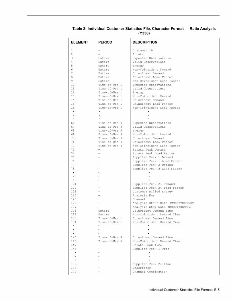
Table 2: Individual Customer Statistics File, Character Format — Ratio Analysis (Y330)
ELEMENT PERIOD DESCRIPTION
12345678910111213141516 • • •66676869707172737475767778 • • •121122123124125126127128129130131 • • •145146147148 • • •172173174
——EntireEntireEntireEntireEntireEntireEntireTime-of-Use 1Time-of-Use 1Time-of-Use 1Time-of-Use 1Time-of-Use 1Time-of-Use 1Time-of-Use 1 • • •Time-of-Use 9Time-of-Use 9Time-of-Use 9Time-of-Use 9Time-of-Use 9Time-of-Use 9Time-of-Use 9——————•••———————EntireEntireTime-of-Use 1Time-of-Use 1•••Time-of-Use 9Time-of-Use 9——•••———
Customer IDStrataExpected ObservationsValid ObservationsEnergyNon-Coincident DemandCoincident DemandCoincident Load FactorNon-Coincident Load FactorExpected ObservationsValid ObservationsEnergyNon-Coincident DemandCoincident DemandCoincident Load FactorNon-Coincident Load Factor • • •Expected ObservationsValid ObservationsEnergyNon-Coincident DemandCoincident DemandCoincident Load FactorNon-Coincident Load FactorStrata Peak DemandStrata Peak Load FactorSupplied Peak 1 DemandSupplied Peak 1 Load FactorSupplied Peak 2 DemandSupplied Peak 2 Load Factor • • •Supplied Peak 24 DemandSupplied Peak 24 Load FactorCustomer Billed EnergyAnalysis KeyChannelAnalysis Start Date (MMDDYYHHMMSS)Analysis Stop Date (MMDDYYHHMMSS)Coincident Demand TimeNon-Coincident Demand TimeCoincident Demand TimeNon-Coincident Demand Time • • •Coincident Demand TimeNon-Coincident Demand TimeStrata Peak TimeSupplied Peak 1 Time • • •Supplied Peak 24 TimeDescriptorChannel Combination
Individual Customer Statistics File Formats E-5
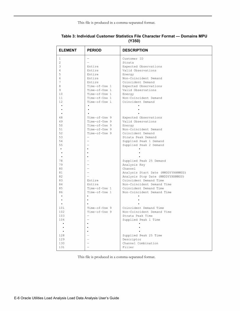
This file is produced in a comma-separated format.
This file is produced in a comma-separated format.
Table 3: Individual Customer Statistics File Character Format — Domains MPU (Y350)
ELEMENT PERIOD DESCRIPTION
123456789101112 • • •4849505152535455 • • •787980818283848586 • • •101102103104 • • •128129130131
——EntireEntireEntireEntireEntireTime-of-Use 1Time-of-Use 1Time-of-Use 1Time-of-Use 1Time-of-Use 1 • • •Time-of-Use 9Time-of-Use 9Time-of-Use 9Time-of-Use 9Time-of-Use 9———•••—————EntireEntireTime-of-Use 1Time-of-Use 1•••Time-of-Use 9Time-of-Use 9——•••————
Customer IDStrataExpected ObservationsValid ObservationsEnergyNon-Coincident DemandCoincident DemandExpected ObservationsValid ObservationsEnergyNon-Coincident DemandCoincident Demand • • •Expected ObservationsValid ObservationsEnergyNon-Coincident DemandCoincident DemandStrata Peak DemandSupplied Peak 1 DemandSupplied Peak 2 Demand • • •Supplied Peak 25 DemandAnalysis KeyChannelAnalysis Start Date (MMDDYYHHMMSS)Analysis Stop Date (MMDDYYHHMMSS)Coincident Demand TimeNon-Coincident Demand TimeCoincident Demand TimeNon-Coincident Demand Time • • •Coincident Demand TimeNon-Coincident Demand TimeStrata Peak TimeSupplied Peak 1 Time • • •Supplied Peak 25 TimeDescriptorChannel CombinationFiller
E-6 Oracle Utilities Load Analysis Load Data Analysis User’s Guide
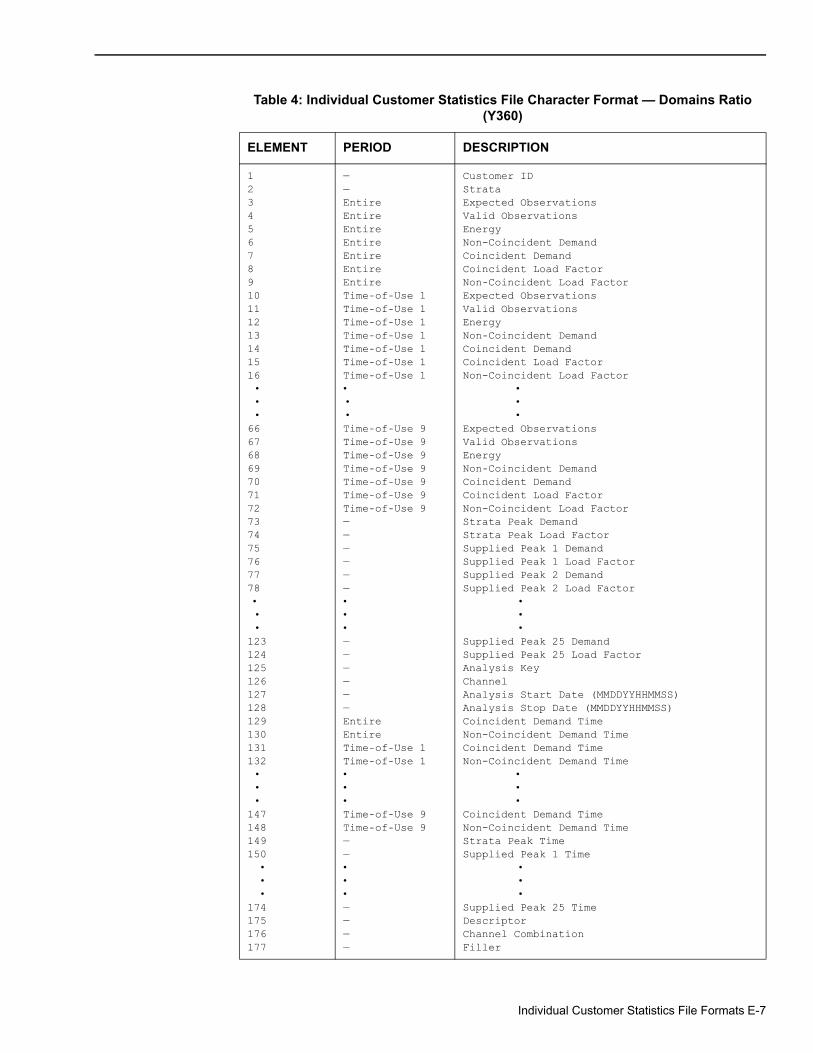
Table 4: Individual Customer Statistics File Character Format — Domains Ratio (Y360)
ELEMENT PERIOD DESCRIPTION
12345678910111213141516 • • •66676869707172737475767778 • • •123124125126127128129130131132 • • •147148149150 • • •174175176177
——EntireEntireEntireEntireEntireEntireEntireTime-of-Use 1Time-of-Use 1Time-of-Use 1Time-of-Use 1Time-of-Use 1Time-of-Use 1Time-of-Use 1• • •Time-of-Use 9Time-of-Use 9Time-of-Use 9Time-of-Use 9Time-of-Use 9Time-of-Use 9Time-of-Use 9——————•••——————EntireEntireTime-of-Use 1Time-of-Use 1•••Time-of-Use 9Time-of-Use 9——•••————
Customer IDStrataExpected ObservationsValid ObservationsEnergyNon-Coincident DemandCoincident DemandCoincident Load FactorNon-Coincident Load FactorExpected ObservationsValid ObservationsEnergyNon-Coincident DemandCoincident DemandCoincident Load FactorNon-Coincident Load Factor • • •Expected ObservationsValid ObservationsEnergyNon-Coincident DemandCoincident DemandCoincident Load FactorNon-Coincident Load FactorStrata Peak DemandStrata Peak Load FactorSupplied Peak 1 DemandSupplied Peak 1 Load FactorSupplied Peak 2 DemandSupplied Peak 2 Load Factor • • •Supplied Peak 25 DemandSupplied Peak 25 Load FactorAnalysis KeyChannelAnalysis Start Date (MMDDYYHHMMSS)Analysis Stop Date (MMDDYYHHMMSS)Coincident Demand TimeNon-Coincident Demand TimeCoincident Demand TimeNon-Coincident Demand Time • • •Coincident Demand TimeNon-Coincident Demand TimeStrata Peak TimeSupplied Peak 1 Time • • •Supplied Peak 25 TimeDescriptorChannel CombinationFiller
Individual Customer Statistics File Formats E-7

This file is produced in a comma-separated format.
E-8 Oracle Utilities Load Analysis Load Data Analysis User’s Guide

Table 5: Individual Customer Statistics File Character Format — 100% Sample Analysis (Y380)
ELEMENT PERIOD DESCRIPTION
12345678910111213141516 • • •66676869707172737475767778 • • •123124125126127128129130131132 • • •147148149150 • • •174175176177
——EntireEntireEntireEntireEntireEntireEntireTime-of-Use 1Time-of-Use 1Time-of-Use 1Time-of-Use 1Time-of-Use 1Time-of-Use 1Time-of-Use 1• • •Time-of-Use 9Time-of-Use 9Time-of-Use 9Time-of-Use 9Time-of-Use 9Time-of-Use 9Time-of-Use 9——————•••——————EntireEntireTime-of-Use 1Time-of-Use 1•••Time-of-Use 9Time-of-Use 9——•••————
Customer IDStrataExpected ObservationsValid ObservationsEnergyNon-Coincident DemandCoincident DemandCoincident Load FactorNon-Coincident Load FactorExpected ObservationsValid ObservationsEnergyNon-Coincident DemandCoincident DemandCoincident Load FactorNon-Coincident Load Factor • • •Expected ObservationsValid ObservationsEnergyNon-Coincident DemandCoincident DemandCoincident Load FactorNon-Coincident Load FactorStrata Peak DemandStrata Peak Load FactorSupplied Peak 1 DemandSupplied Peak 1 Load FactorSupplied Peak 2 DemandSupplied Peak 2 Load Factor • • •Supplied Peak 25 DemandSupplied Peak 25 Load FactorAnalysis KeyChannelAnalysis Start Date (MMDDYYHHMMSS)Analysis Stop Date (MMDDYYHHMMSS)Coincident Demand TimeNon-Coincident Demand TimeCoincident Demand TimeNon-Coincident Demand Time • • •Coincident Demand TimeNon-Coincident Demand TimeStrata Peak TimeSupplied Peak 1 Time • • •Supplied Peak 25 TimeDescriptorChannel CombinationFiller
Individual Customer Statistics File Formats E-9

This file is produced in a comma-separated format.
E-10 Oracle Utilities Load Analysis Load Data Analysis User’s Guide

Appendix FCoincident Peak Analysis Equations
This appendix documents the coincident peak analysis calculations used in the Coincident Peak Analysis Program. This material assumes a basic understanding of statistics, load research calculations, and Oracle Utilities Load Analysis’s operation.
F.1 Non-Stratified Coincident Peak Analysis Equations (Mean-Per-Unit)
Let:ijbjNjyjiCjiC
=======
customer index, i = 1, 2, ..., I;period index, j = 1, 2, ..., J (J < 12);j-th period’s weight;total population for period j;i-th customer’s demand (KW) for period j;i-th customer’s status code (hexadecimal) for period j;worst acceptable status code;
Define:
Xji1 if Cji C;≤
0 otherwise.
=
Coincident Peak Analysis Equations F-1
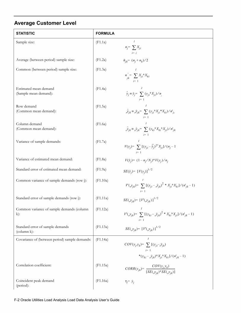
Average Customer Level
STATISTIC FORMULA
Sample size: (F1.1a)
Average (between period) sample size: (F1.2a)
Common (between period) sample size: (F1.3a)
Estimated mean demand(Sample mean demand):
(F1.4a)
Row demand(Common mean demand):
(F1.5a)
Column demand(Common mean demand):
(F1.6a)
Variance of sample demands: (F1.7a)
Variance of estimated mean demand: (F1.8a)
Standard error of estimated mean demand: (F1.9a)
Common variance of sample demands (row j): (F1.10a)
Standard error of sample demands (row j): (F1.11a)
Common variance of sample demands (column k):
(F1.12a)
Standard error of sample demands (column k):
(F1.13a)
Covariance of (between period) sample demands: (F1.14a)
Correlation coefficient: (F1.15a)
Coincident peak demand(period):
(F1.16a)
nj Xjii j=
l
=
njk nj nk+( ) 2⁄=
n 'jk
Xji∗Xkii 1=
I
=
yj yj yji∗Xji( )i 1=
I
=≡ nj⁄
yr jk yr jk yji∗Xji*Xki( ) n'jk⁄
i 1=
I
=≡
yc jk yc jk yki∗Xki∗Xji( ) n'jk⁄i 1=
I
=≡
V yj( ) yji yj–( )2∗Xji[ ] nj 1–( )⁄i 1=
I
=
V yj( ) 1 nj Nj⁄–( )∗V yj ) nj⁄(=
SE yj( ) V yj( )[ ]1 2⁄=
V' yr jk( ) yji yr jk–( )2 * Xji∗Xki[ ] n'jk 1–( )⁄i 1=
I
=
SE yr jk( ) V' yr jk )([ ]1 2⁄=
V' yc jk( ) yki yc jk–( )2 * Xki∗Xji[ ] n'jk 1–( )⁄i 1=
I
=
SE yc jk( ) V' yc jk )([ ]1 2⁄=
COV yj ,yk( ) yji yr jk–( )[i 1=
I
=
* yki yc jk–( )∗Xji∗Xki ] n'jk 1–( )⁄
CORR yjk( )COV yj ,yk( )
SE yr jk( )∗SE yc jk( )[ ]-------------------------------------------------=
τj yj=
F-2 Oracle Utilities Load Analysis Load Data Analysis User’s Guide
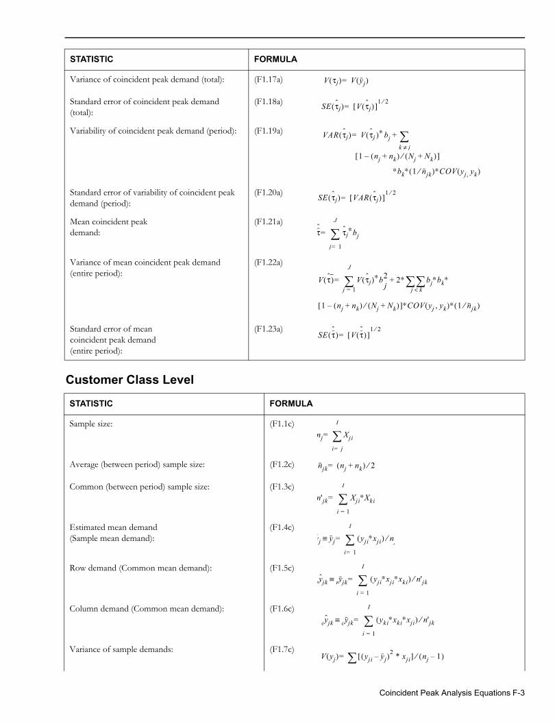
Customer Class Level
Variance of coincident peak demand (total): (F1.17a)
Standard error of coincident peak demand (total):
(F1.18a)
Variability of coincident peak demand (period): (F1.19a)
Standard error of variability of coincident peak demand (period):
(F1.20a)
Mean coincident peakdemand:
(F1.21a)
Variance of mean coincident peak demand (entire period):
(F1.22a)
Standard error of meancoincident peak demand(entire period):
(F1.23a)
STATISTIC FORMULA
Sample size: (F1.1c)
Average (between period) sample size: (F1.2c)
Common (between period) sample size: (F1.3c)
Estimated mean demand(Sample mean demand):
(F1.4c)
Row demand (Common mean demand): (F1.5c)
Column demand (Common mean demand): (F1.6c)
Variance of sample demands: (F1.7c)
STATISTIC FORMULA
V τj( ) V yj( )=
SE τj( ) V τj( )[ ]1 2⁄
=
VAR τj( ) V τj )∗( bj k j≠+=
1 nj nk+( ) Nj Nk+( )⁄–[ ]
∗bk∗ 1 njk⁄( )∗COV yj , yk( )
SE τj( ) VAR τj( )[ ]1 2⁄
=
τˆ
τj∗bjj 1=
J
=
V τ( ) V τj( )∗b
2j
2∗ bj∗bk∗j k<+
j 1=
J
=
1 nj nk+( ) Nj Nk+( )⁄–[ ]∗COV yj yk,( )∗ 1 njk⁄( )
SE τˆ
( ) V τˆ
( )[ ]1 2⁄
=
nj Xjii j=
I
=
njk nj nk+( ) 2⁄=
n'jk Xji∗Xkii 1=
I
=
yj yj yji∗xji( ) nj⁄i 1=
I
=≡
yr jk yr jk yji∗xji∗xki( ) n'jk⁄i 1=
I
=≡
yc jk yc jk yki∗xki∗xji( ) n'jk⁄i 1=
I
=≡
V yj( ) yji yj–( )2 * xji[ ] nj 1–( )⁄=
Coincident Peak Analysis Equations F-3
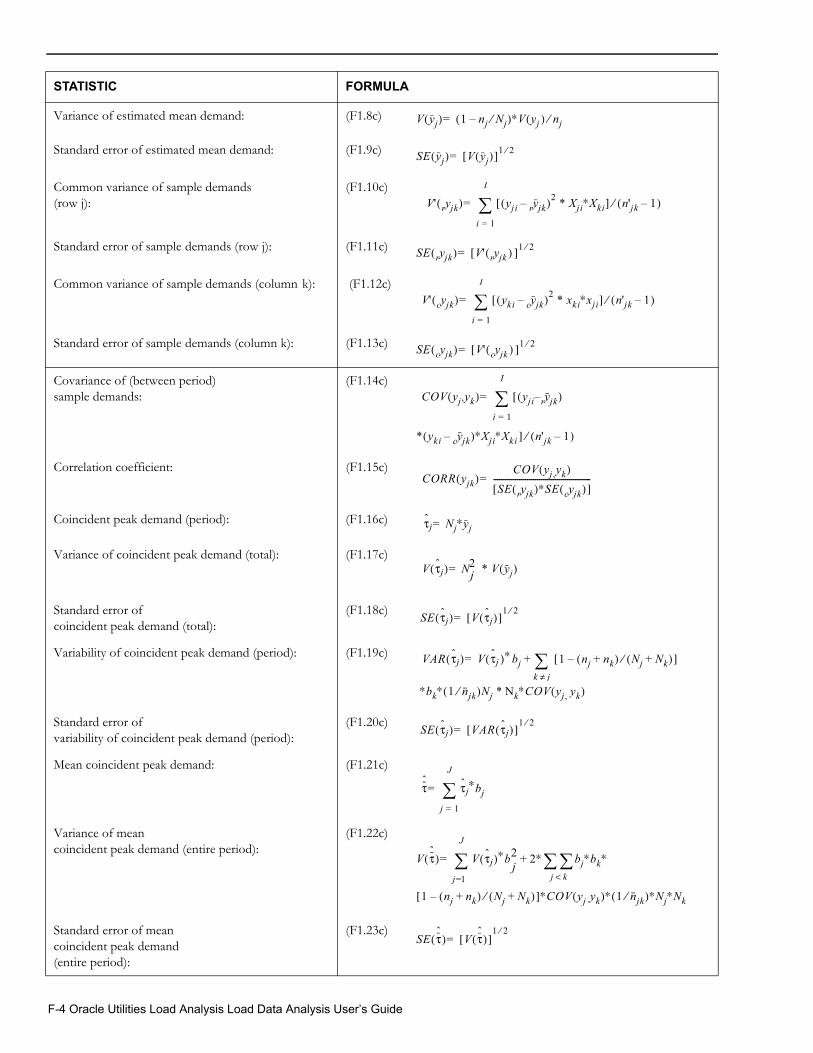
Variance of estimated mean demand: (F1.8c)
Standard error of estimated mean demand: (F1.9c)
Common variance of sample demands (row j):
(F1.10c)
Standard error of sample demands (row j): (F1.11c)
Common variance of sample demands (column k): (F1.12c)
Standard error of sample demands (column k): (F1.13c)
Covariance of (between period) sample demands:
(F1.14c)
Correlation coefficient: (F1.15c)
Coincident peak demand (period): (F1.16c)
Variance of coincident peak demand (total): (F1.17c)
Standard error ofcoincident peak demand (total):
(F1.18c)
Variability of coincident peak demand (period): (F1.19c)
Standard error ofvariability of coincident peak demand (period):
(F1.20c)
Mean coincident peak demand: (F1.21c)
Variance of meancoincident peak demand (entire period):
(F1.22c)
Standard error of meancoincident peak demand(entire period):
(F1.23c)
STATISTIC FORMULA
V yj( ) 1 nj Nj⁄–( )∗V yj ) nj⁄(=
SE yj( ) V yj( )[ ]1 2⁄=
V' yr jk( ) yji yr jk–( )2 * Xji∗Xki[ ] n'jk 1–( )⁄i 1=
I
=
SE yr jk( ) V' yr jk )([ ]1 2⁄=
V' yc jk( ) yki yc jk–( )2 * xki∗xji[ ] n'jk 1–( )⁄i 1=
I
=
SE yc jk( ) V' yc jk )([ ]1 2⁄=
COV yj ,yk( ) yji yr jk–( )[i 1=
I
=
* yki yc jk–( )∗Xji∗Xki ] n'jk 1–( )⁄
CORR yjk( )COV yj ,yk( )
SE yr jk( )∗SE yc jk( )[ ]-------------------------------------------------=
τj Nj∗yj=
V τj( ) N2j * V yj( )=
SE τj( ) V τj( )[ ]1 2⁄=
VAR τj( ) V τj )∗( bj k j≠+= 1 nj nk+( ) Nj Nk+( )⁄–[ ]
∗bk∗ 1 njk⁄( )Nj * Nk∗COV yj , yk( )
SE τj( ) VAR τj( )[ ]1 2⁄
=
τˆ
τj∗bjj 1=
J
=
V τˆ
( ) V τj( )∗b
2j
2∗ bj∗bk∗j k<+
j 1=
J
=
1 nj nk+( ) Nj Nk+( )⁄–[ ]∗COV yj ,yk( )∗ 1 njk⁄( )∗Nj∗Nk
SE τˆ
( ) V τˆ
( )[ ]1 2⁄
=
F-4 Oracle Utilities Load Analysis Load Data Analysis User’s Guide
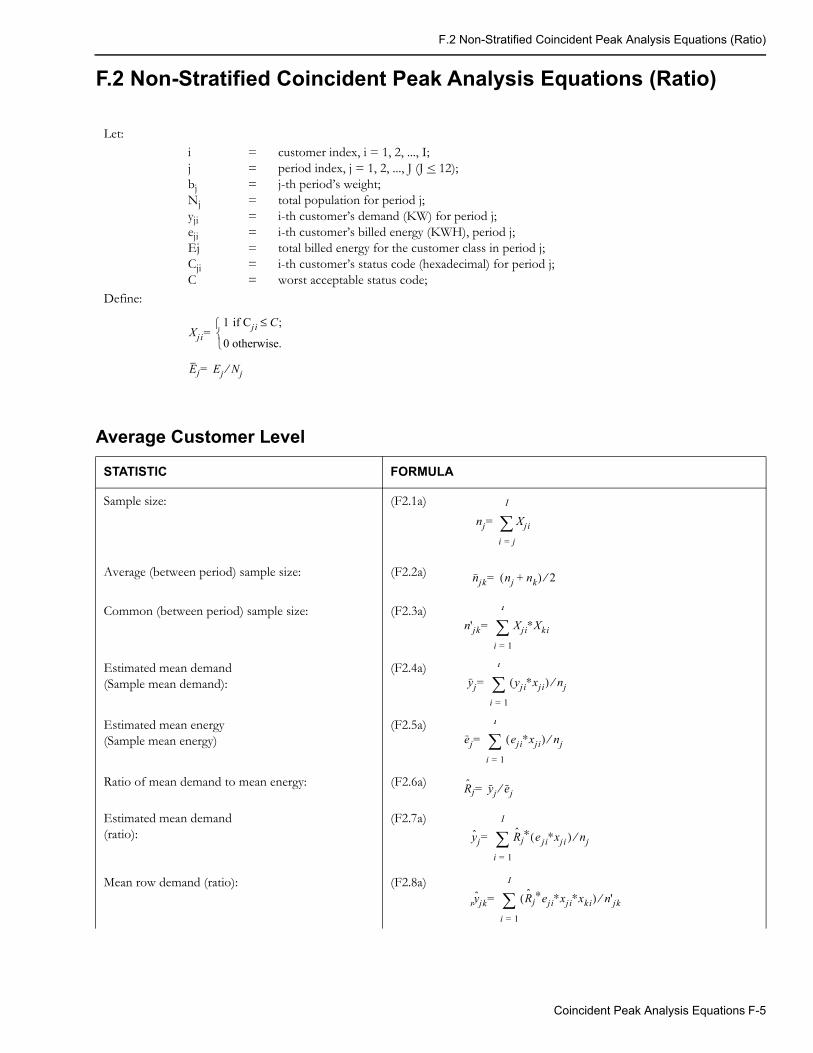
F.2 Non-Stratified Coincident Peak Analysis Equations (Ratio)
F.2 Non-Stratified Coincident Peak Analysis Equations (Ratio)
Average Customer Level
Let:ijbjNjyjiejiEjCjiC
=========
customer index, i = 1, 2, ..., I;period index, j = 1, 2, ..., J (J < 12);j-th period’s weight;total population for period j;i-th customer’s demand (KW) for period j;i-th customer’s billed energy (KWH), period j;total billed energy for the customer class in period j;i-th customer’s status code (hexadecimal) for period j;worst acceptable status code;
Define:
Xji1 if Cji C;≤
0 otherwise.
=
Ej Ej Nj⁄=
STATISTIC FORMULA
Sample size: (F2.1a)
Average (between period) sample size: (F2.2a)
Common (between period) sample size: (F2.3a)
Estimated mean demand(Sample mean demand):
(F2.4a)
Estimated mean energy (Sample mean energy)
(F2.5a)
Ratio of mean demand to mean energy: (F2.6a)
Estimated mean demand(ratio):
(F2.7a)
Mean row demand (ratio): (F2.8a)
nj Xjii j=
I
=
njk nj nk+( ) 2⁄=
n'jk Xji∗Xkii 1=
I
=
yj yji∗xji( ) nj⁄i 1=
I
=
ej eji∗xji( ) nj⁄i 1=
I
=
Rj yj ej⁄=
yj Rj∗ e( ji∗xji ) nj⁄
i 1=
I
=
yr jk Rj∗eji∗xji∗xki( ) n'jk⁄i 1=
I
=
Coincident Peak Analysis Equations F-5
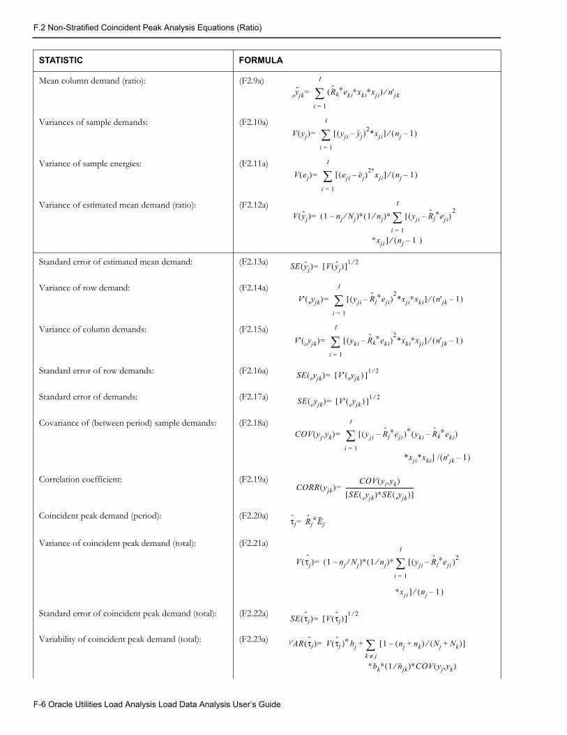
F.2 Non-Stratified Coincident Peak Analysis Equations (Ratio)
Mean column demand (ratio): (F2.9a)
Variances of sample demands: (F2.10a)
Variance of sample energies: (F2.11a)
Variance of estimated mean demand (ratio): (F2.12a)
Standard error of estimated mean demand: (F2.13a)
Variance of row demand: (F2.14a)
Variance of column demands: (F2.15a)
Standard error of row demands: (F2.16a)
Standard error of demands: (F2.17a)
Covariance of (between period) sample demands: (F2.18a)
Correlation coefficient: (F2.19a)
Coincident peak demand (period): (F2.20a)
Variance of coincident peak demand (total): (F2.21a)
Standard error of coincident peak demand (total): (F2.22a)
Variability of coincident peak demand (total): (F2.23a)
STATISTIC FORMULA
yc jk Rk∗eki∗xki∗xji( ) n'jk⁄
i 1=
I
=
V yj( ) yji yj–( )2*xji[ ] nj 1–( )⁄i 1=
I
=
V ej( ) eji ej–( )2∗xji[ ] nj 1–( )⁄
i 1=
I
=
V yj( ) 1 nj Nj⁄–( )∗ 1 nj⁄( )∗ yji Rj∗eji–( )[2
i 1=
I
=
∗xji ] nj 1– ( )⁄
SE yj( ) V yj( )[ ]1 2⁄=
V' yr jk( ) yji Rj∗eji–( )2*xji∗xki[ ] n'jk 1–( )⁄
i 1=
I
=
V' yc jk( ) yki Rk∗eki–( )2*xki∗xji[ ] n'jk 1–( )⁄
i 1=
I
=
SE yr jk( ) V' yr jk )([ ]1 2⁄=
SE yc jk( ) V' yc jk )([ ]1 2⁄=
COV yj ,yk( ) y( j i[ Rj∗eji )– ∗ yki Rk∗eki–( )i 1=
I
=
*xji*xki] / n'jk 1–( )
CORR yjk( )COV yi,yk( )
SE yc jk( )∗SE yr jk( )[ ]-------------------------------------------------=
τj Rj∗Ej=
V τjˆ( ) 1 nj Nj⁄–( )∗ 1 nj⁄( )∗ yji Rj∗eji )
2–([i 1=
I
=
∗xji ] nj 1 )–(⁄
SE τj( ) V τj( )[ ]1 2⁄=
VAR τj( ) V τj )∗( bj k j≠+= 1 nj nk+( ) Nj Nk+( )⁄–[ ]
∗bk∗ 1 njk⁄( )∗COV yj,yk( )
F-6 Oracle Utilities Load Analysis Load Data Analysis User’s Guide
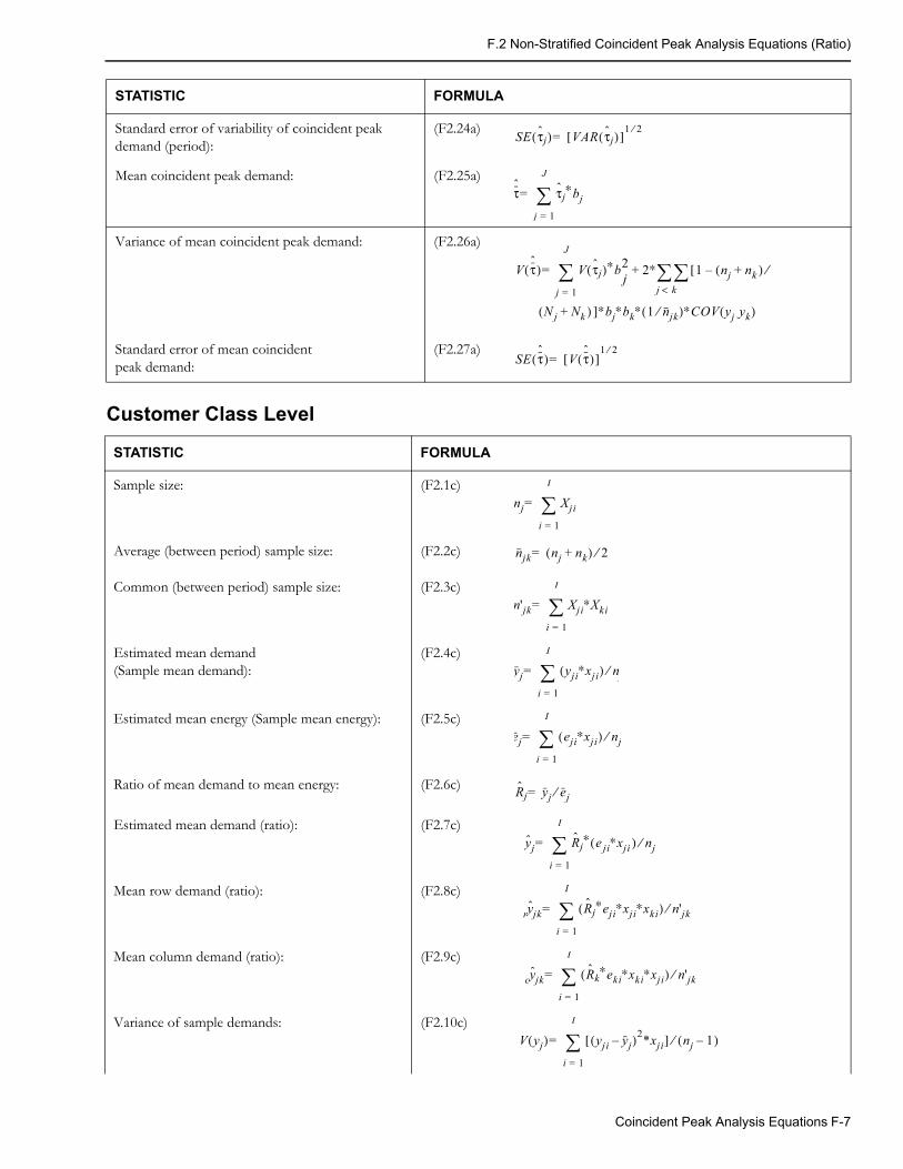
F.2 Non-Stratified Coincident Peak Analysis Equations (Ratio)
Customer Class Level
Standard error of variability of coincident peak demand (period):
(F2.24a)
Mean coincident peak demand: (F2.25a)
Variance of mean coincident peak demand: (F2.26a)
Standard error of mean coincident peak demand:
(F2.27a)
STATISTIC FORMULA
Sample size: (F2.1c)
Average (between period) sample size: (F2.2c)
Common (between period) sample size: (F2.3c)
Estimated mean demand(Sample mean demand):
(F2.4c)
Estimated mean energy (Sample mean energy): (F2.5c)
Ratio of mean demand to mean energy: (F2.6c)
Estimated mean demand (ratio): (F2.7c)
Mean row demand (ratio): (F2.8c)
Mean column demand (ratio): (F2.9c)
Variance of sample demands: (F2.10c)
STATISTIC FORMULA
SE τj( ) VAR τj( )[ ]1 2⁄=
τˆ
τj∗bjj 1=
J
=
V τˆ
( ) V τj( )∗b
2j
2∗ 1 nj nk ) ⁄+(–[k
j <+
j 1=
J
=
N( j Nk ) ]+ ∗bj∗bk∗ 1 njk⁄( )∗COV yj ,yk( )
SE τˆ
( ) V τˆ
( )[ ]1 2⁄
=
nj Xjii 1=
I
=
njk nj nk+( ) 2⁄=
n'jk Xji∗Xkii 1=
I
=
yj yji∗xji( ) nj⁄
i 1=
I
=
ej eji∗xji( ) nj⁄i 1=
I
=
Rj yj ej⁄=
yj Rj∗ e( ji∗xji ) nj⁄i 1=
I
=
yr jk Rj∗eji∗xji∗xki( ) n'jk⁄
i 1=
I
=
yc jk Rk∗eki∗xki∗xji( ) n'jk⁄i 1=
I
=
V yj( ) yji yj–( )2*xji[ ] nj 1–( )⁄i 1=
I
=
Coincident Peak Analysis Equations F-7
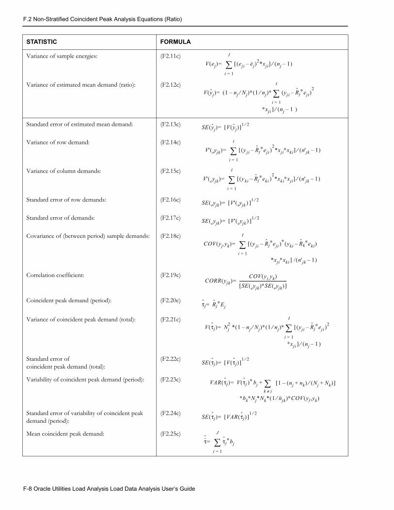
F.2 Non-Stratified Coincident Peak Analysis Equations (Ratio)
Variance of sample energies: (F2.11c)
Variance of estimated mean demand (ratio): (F2.12c)
Standard error of estimated mean demand: (F2.13c)
Variance of row demand: (F2.14c)
Variance of column demands: (F2.15c)
Standard error of row demands: (F2.16c)
Standard error of demands: (F2.17c)
Covariance of (between period) sample demands: (F2.18c)
Correlation coefficient: (F2.19c)
Coincident peak demand (period): (F2.20c)
Variance of coincident peak demand (total): (F2.21c)
Standard error ofcoincident peak demand (total):
(F2.22c)
Variability of coincident peak demand (period): (F2.23c)
Standard error of variability of coincident peak demand (period):
(F2.24c)
Mean coincident peak demand: (F2.25c)
STATISTIC FORMULA
V ej( ) eji ej–( )2*xji[ ] nj 1–( )⁄
i 1=
I
=
V yj( ) 1 nj Nj⁄–( )∗ 1 nj⁄( )∗ yji Rj∗eji–( )2
i 1=
I
=
∗xji ] nj 1– ( )⁄
SE yj( ) V yj( )[ ]1 2⁄=
V' yr jk( ) y( ji Rj∗eji )–2*xji∗xki[ ] n'jk 1–( )⁄
i 1=
I
=
V' yc jk( ) y( ki Rj∗eki )–2*xki∗xji[ ] n'jk 1–( )⁄
i 1=
I
=
SE yr jk( ) V' yr jk )([ ]1 2⁄=
SE yc jk( ) V' yc jk )([ ]1 2⁄=
COV yj ,yk( ) y( ji[ Rj∗eji )– ∗ yki Rk∗eki–( )i 1=
I
=
*xji∗xki ] / n'jk 1–( )
CORR yjk( )COV yi ,yk( )
SE yc jk( )∗SE yr jk( )[ ]-------------------------------------------------=
τj Rj∗Ej=
V τj( ) Nj2 * 1 nj Nj⁄–( )∗ 1 nj⁄( )∗ yji Rj∗eji )
2–([
i 1=
I
=
∗xji ] nj 1 )–(⁄
SE τj( ) V τj( )[ ]1 2⁄=
VAR τj( ) V τj )∗( bj k j≠+= 1 nj nk+( ) Nj Nk+( )⁄–[ ]
∗bk∗Nj*Nk* 1 njk⁄( )∗COV yj,yk( )
SE τj( ) VAR τj( )[ ]1 2⁄
=
τˆ
τj∗bjj 1=
J
=
F-8 Oracle Utilities Load Analysis Load Data Analysis User’s Guide
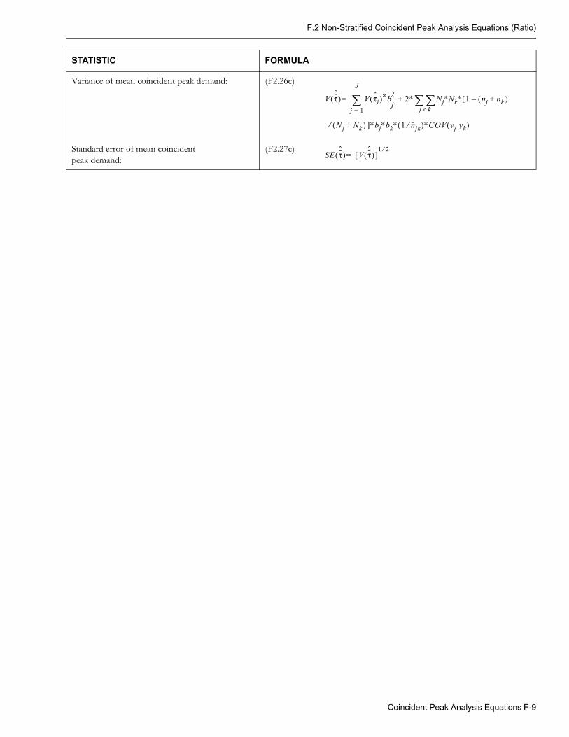
F.2 Non-Stratified Coincident Peak Analysis Equations (Ratio)
Variance of mean coincident peak demand: (F2.26c)
Standard error of mean coincident peak demand:
(F2.27c)
STATISTIC FORMULA
V τˆ
( ) V τj( )∗b
2j
2∗ Nj∗Nk∗ 1 nj nk )+(–[j k<+
j 1=
J
=
N( j⁄ Nk ) ]+ ∗bj∗bk∗ 1 njk⁄( )∗COV yj ,yk( )
SE τˆ
( ) V τˆ
( )[ ]1 2⁄
=
Coincident Peak Analysis Equations F-9
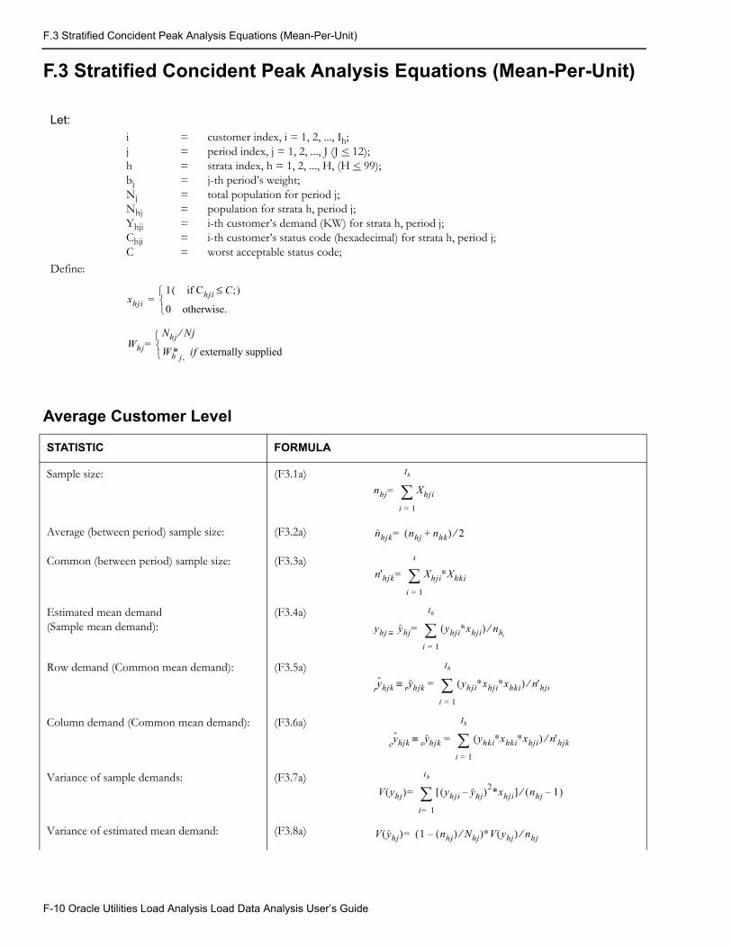
F.3 Stratified Concident Peak Analysis Equations (Mean-Per-Unit)
F.3 Stratified Concident Peak Analysis Equations (Mean-Per-Unit)
Average Customer Level
Let:ijhbjNjNhjYhjiChjiC
=========
customer index, i = 1, 2, ..., Ih;period index, j = 1, 2, ..., J (J < 12);strata index, h = 1, 2, ..., H, (H < 99);j-th period’s weight;total population for period j;population for strata h, period j;i-th customer’s demand (KW) for strata h, period j;i-th customer’s status code (hexadecimal) for strata h, period j;worst acceptable status code;
Define:
xhji1 if Chji C;≤( )
0 otherwise.
=
WhjNhj Nj⁄
Wh* j , if externally supplied
=
STATISTIC FORMULA
Sample size: (F3.1a)
Average (between period) sample size: (F3.2a)
Common (between period) sample size: (F3.3a)
Estimated mean demand(Sample mean demand):
(F3.4a)
Row demand (Common mean demand): (F3.5a)
Column demand (Common mean demand): (F3.6a)
Variance of sample demands: (F3.7a)
Variance of estimated mean demand: (F3.8a)
nhj Xhjii 1=
Ih
=
nhjk nhj nhk+( ) 2⁄=
n'hjk Xhji∗Xhkii 1=
I
=
yhj ≡ yhj yhji∗xhji( ) nhj⁄i 1=
Ih
=
yhjkr yr hjk≡ yhji∗xhji∗xhki( ) n'hjk⁄
i 1=
Ih
=
yhjkc yc hjk≡ yhki∗xhki∗xhji( ) n'hjk⁄i 1=
Ih
=
V yhj( ) yhji yhj–( )2*xhji[ ] nhj 1–( )⁄i 1=
Ih
=
V yhj( ) 1 nhj( ) Nhj⁄–( )∗V yhj( ) nhj⁄=
F-10 Oracle Utilities Load Analysis Load Data Analysis User’s Guide
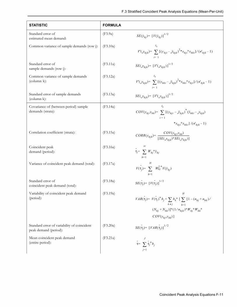
F.3 Stratified Concident Peak Analysis Equations (Mean-Per-Unit)
Standard error ofestimated mean demand:
(F3.9a)
Common variance of sample demands (row j): (F3.10a)
Standard error ofsample demands (row j):
(F3.11a)
Common variance of sample demands (column k):
(F3.12a)
Standard error of sample demands (column k):
(F3.13a)
Covariance of (between period) sample demands (strata):
(F3.14a)
Correlation coefficient (strata): (F3.15a)
Coincident peakdemand (period):
(F3.16a)
Variance of coincident peak demand (total): (F3.17a)
Standard error ofcoincident peak demand (total):
(F3.18a)
Variability of coincident peak demand (period):
(F3.19a)
Standard error of variability of coincident peak demand (period):
(F3.20a)
Mean coincident peak demand (entire period):
(F3.21a)
STATISTIC FORMULA
SE yhj( ) V yhj( )[ ]1 2⁄=
V' yr hjk( ) y( hji yr hjk )– 2*xhji∗xhki[ ] n'hjk 1–( )⁄i 1=
Ih
=
SE yr hjk( ) V' yr hjk )([ ]1 2⁄=
V' yc hjk( ) yhki yc hjk–( )2*xhki∗xhji[ ] n'hjk 1–( )⁄i 1=
Ih
=
SE yc hjk( ) V' yc hjk )([ ]1 2⁄=
COV yhj ,yhk( ) yhji([ yr hjk )– ∗ yhki yc hjk–( )i 1=
Ih
=
*xhji∗xhki ] / n'hjk 1–( )
CORR yhjk( )COV yhj,yhk( )
SE yr hjk( )∗SE yc hjk( )[ ]------------------------------------------------------=
τj Whj∗yhjh 1=
H
=
V τjˆ( ) W2
hj∗V yhj( )
h 1=
H
=
SE τj( ) V τj( )[ ]1 2⁄
=
VAR τj( ) V τj )∗( bj bk∗ [ 1 nhj nhk ) ⁄+(–[h 1=
H
k j≠+=
Nhj( Nhk )]∗ 1 nhjk⁄ )∗Whj∗Whk∗(+
COV yhj,yhk( ) ]
SE τj( ) VAR τj( )[ ]1 2⁄=
τ τj∗bjj 1=
J
=
Coincident Peak Analysis Equations F-11
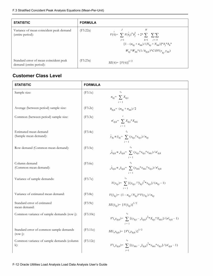
F.3 Stratified Concident Peak Analysis Equations (Mean-Per-Unit)
Customer Class Level
Variance of mean coincident peak demand (entire period):
(F3.22a)
Standard error of mean coincident peak demand (entire period):
(F3.23a)
STATISTIC FORMULA
Sample size: (F3.1c)
Average (between period) sample size: (F3.2c)
Common (between period) sample size: (F3.3c)
Estimated mean demand(Sample mean demand):
(F3.4c)
Row demand (Common mean demand): (F3.5c)
Column demand (Common mean demand):
(F3.6c)
Variance of sample demands: (F3.7c)
Variance of estimated mean demand: (F3.8c)
Standard error of estimated mean demand:
(F3.9c)
Common variance of sample demands (row j): (F3.10c)
Standard error of common sample demands (row j):
(F3.11c)
Common variance of sample demands (column k):
(F3.12c)
STATISTIC FORMULA
V τˆ
( ) V τj( )∗bj2 2∗
j k<
h 1=
H
+j 1=
J
=
1 nhj nhk+( ) Nhj Nhk+( )⁄–[ ]∗bj∗bk∗
Whj∗Whk∗ 1 nhjk⁄ )∗C( OV yhj ,yhk( )
SE τ( ) V τ( )[ ]1 2⁄=
nhj Xhjii 1=
Ih
=
nhjk nhj nhk+( ) 2⁄=
n'hjk Xhji∗Xhkii 1=
I
=
yhj yhj yhji∗xhji( ) nhj⁄i 1=
Ih
=≡
yr hjk yr hjk yhji∗xhji∗xhki( ) n'hjk⁄i 1=
Ih
=≡
yc hjk yc hjk yhki∗xhki∗xhji( ) n'hjk⁄i 1=
Ih
=≡
V yhj( ) yhji yhj–( )2*xhji[ ] nhj 1–( )⁄i 1=
Ih
=
V yhj( ) 1 nhj Nhj⁄–( )∗V yhj ) nhj⁄(=
SE yhj( ) V yhj( )[ ]1 2⁄=
V' yr hjk( ) yhji yr hjk–( )2*Xhji∗Xhki[ ] n'hjk 1–( )⁄i 1=
Ih
=
SE yr hjk( ) V' yr hjk )([ ]1 2⁄=
V' yc hjk( ) yhki yc hjk–( )2*xhki∗xhji[ ] n'hjk 1–( )⁄i 1=
Ih
=
F-12 Oracle Utilities Load Analysis Load Data Analysis User’s Guide
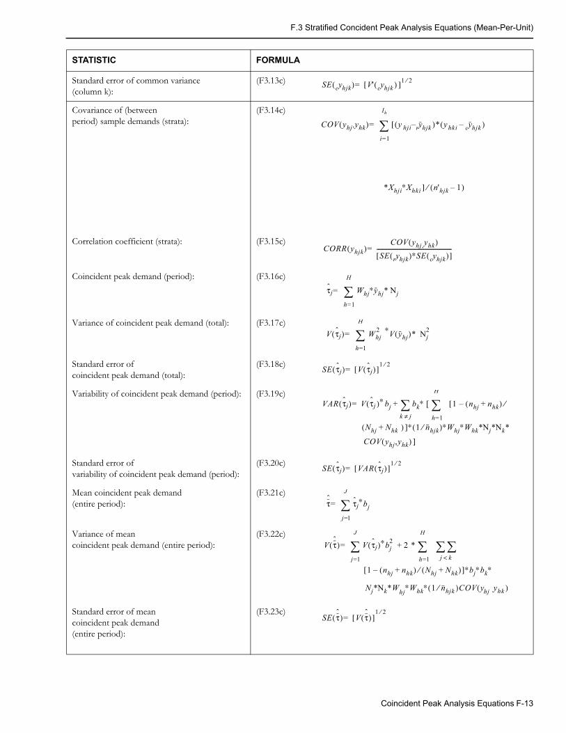
F.3 Stratified Concident Peak Analysis Equations (Mean-Per-Unit)
Standard error of common variance (column k):
(F3.13c)
Covariance of (betweenperiod) sample demands (strata):
(F3.14c)
Correlation coefficient (strata): (F3.15c)
Coincident peak demand (period): (F3.16c)
Variance of coincident peak demand (total): (F3.17c)
Standard error ofcoincident peak demand (total):
(F3.18c)
Variability of coincident peak demand (period): (F3.19c)
Standard error ofvariability of coincident peak demand (period):
(F3.20c)
Mean coincident peak demand (entire period):
(F3.21c)
Variance of meancoincident peak demand (entire period):
(F3.22c)
Standard error of meancoincident peak demand(entire period):
(F3.23c)
STATISTIC FORMULA
SE yc hjk( ) V' yc hjk )([ ]1 2⁄=
COV yhj ,yhk( ) y([ hji yr hjk )* y( hki yc hjk )––i 1=
Ih
=
*Xhji∗Xhki ] n'hjk 1–( )⁄
CORR yhjk( )COV yhj ,yhk( )
SE yr hjk( )∗SE yc hjk( )[ ]------------------------------------------------------=
τj Whj∗yhj* Njh 1=
H
=
V τj( ) Whj2 ∗V yhj( )* Nj
2
h 1=
H
=
SE τj( ) V τj( )[ ]1 2⁄
=
VAR τj( ) V τj )∗( bj bk∗ [ h 1=
H
k j≠+= 1[ nhj nhk+( ) ⁄–
Nhj Nhk+ ( ) ]∗ 1 nhjk⁄( )∗Whj∗Whk*Nj*Nk*
COV yhj,yhk( ) ]
SE τj( ) VAR τj( )[ ]1 2⁄
=
τˆ
τj∗bjj 1=
J
=
V τˆ
( ) V τj( )∗bj2 2 *
j k<
h 1=
H
+j 1=
J
=
1 nhj nhk+( ) Nhj Nhk+( )⁄–[ ]∗bj∗bk∗
Nj*Nk*Whj∗Whk∗ 1 nhjk )⁄ COV y( hj ,yhk )(
SE τˆ
( ) V τˆ
( )[ ]1 2⁄
=
Coincident Peak Analysis Equations F-13
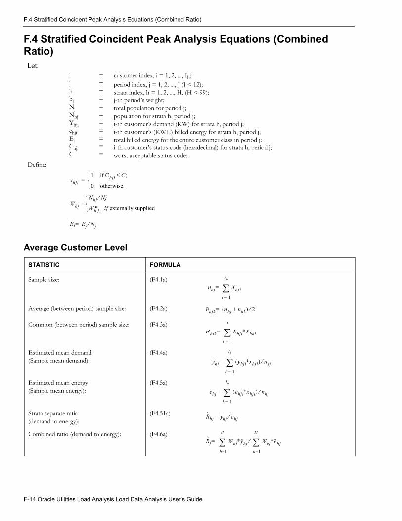
F.4 Stratified Coincident Peak Analysis Equations (Combined Ratio)
F.4 Stratified Coincident Peak Analysis Equations (Combined Ratio)
Average Customer Level
Let:ijhbjNjNhjYhjiehjiEjChjiC
===========
customer index, i = 1, 2, ..., Ih;period index, j = 1, 2, ..., J (J < 12);strata index, h = 1, 2, ..., H, (H < 99);j-th period’s weight;total population for period j;population for strata h, period j;i-th customer’s demand (KW) for strata h, period j;i-th customer’s (KWH) billed energy for strata h, period j;total billed energy for the entire customer class in period j;i-th customer’s status code (hexadecimal) for strata h, period j;worst acceptable status code;
Define:
STATISTIC FORMULA
Sample size: (F4.1a)
Average (between period) sample size: (F4.2a)
Common (between period) sample size: (F4.3a)
Estimated mean demand(Sample mean demand):
(F4.4a)
Estimated mean energy (Sample mean energy):
(F4.5a)
Strata separate ratio (demand to energy):
(F4.51a)
Combined ratio (demand to energy): (F4.6a)
xhji1 if Chji C;≤
0 otherwise.
=
WhjNhj Nj⁄
Wh*j , if externally supplied
=
Ej Ej Nj⁄=
nhj Xhjii 1=
Ih
=
nhjk nhj nhk+( ) 2⁄=
n'hjk Xhji∗Xhkii 1=
I
=
yhj yhji∗xhji( ) nhj⁄i 1=
Ih
=
ehj ehji∗xhji( ) nhj⁄i 1=
Ih
=
Rhj yhj ehj⁄=
Rj Whj∗yhj Whj∗ehjh 1=
H
⁄h 1=
H
=
F-14 Oracle Utilities Load Analysis Load Data Analysis User’s Guide
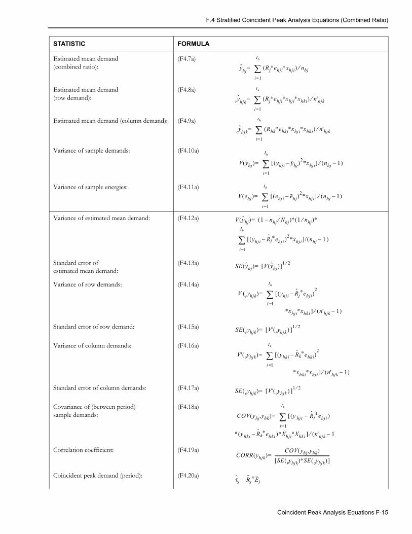
F.4 Stratified Coincident Peak Analysis Equations (Combined Ratio)
Estimated mean demand (combined ratio):
(F4.7a)
Estimated mean demand (row demand):
(F4.8a)
Estimated mean demand (column demand): (F4.9a)
Variance of sample demands: (F4.10a)
Variance of sample energies: (F4.11a)
Variance of estimated mean demand: (F4.12a)
Standard error ofestimated mean demand:
(F4.13a)
Variance of row demands: (F4.14a)
Standard error of row demand: (F4.15a)
Variance of column demands: (F4.16a)
Standard error of column demands: (F4.17a)
Covariance of (between period) sample demands:
(F4.18a)
Correlation coefficient: (F4.19a)
Coincident peak demand (period): (F4.20a)
STATISTIC FORMULA
y hj Rj∗ehji∗xhji( ) nhj⁄i 1=
Ih
=
yr hjk Rj∗ehji∗xhji∗xhki( ) n'hjk⁄i 1=
Ih
=
yc hjk Rhk∗ehki∗xhji∗xhki( ) n'hjk⁄i 1=
Ih
=
V yhj( ) yhji yhj–( )2*xhji[ ] nhj 1–( )⁄i 1=
Ih
=
V ehj( ) ehji ehj–( )2*xhji[ ] nhj 1–( )⁄i 1=
Ih
=
V yhj( ) 1 nhj Nhj⁄–( )∗ 1 nhj⁄( )∗=
yhji Rj∗ehji )2*xhji ]/ nhj 1– )(–([
i 1=
Ih
SE yhj( ) V yhj( )[ ]1 2⁄=
V' yr hjk( ) [ yhji Rj∗ehji–( )2
i 1=
Ih
=
∗xhji∗xhki ] n'hjk 1–( )⁄
SE yr hjk( ) V' yr hjk )([ ]1 2⁄=
V' yc hjk( ) [ yhki Rk∗ehki–( )2
i 1=
Ih
=
∗xhki∗xhji ] n'hjk 1–( )⁄
SE yc hjk( ) V' yc hjk )([ ]1 2⁄=
COV yhj ,yhk( ) y([ hji Rj∗ehji )–i 1=
Ih
=
* y( hki Rk∗ehki )– *Xhji∗Xhki ] n'hjk 1–( )⁄
CORR yhjk( )COV yhj,yhk( )
SE yr hjk( )∗SE yc hjk( )[ ]------------------------------------------------------=
τj Rj∗Ej=
Coincident Peak Analysis Equations F-15
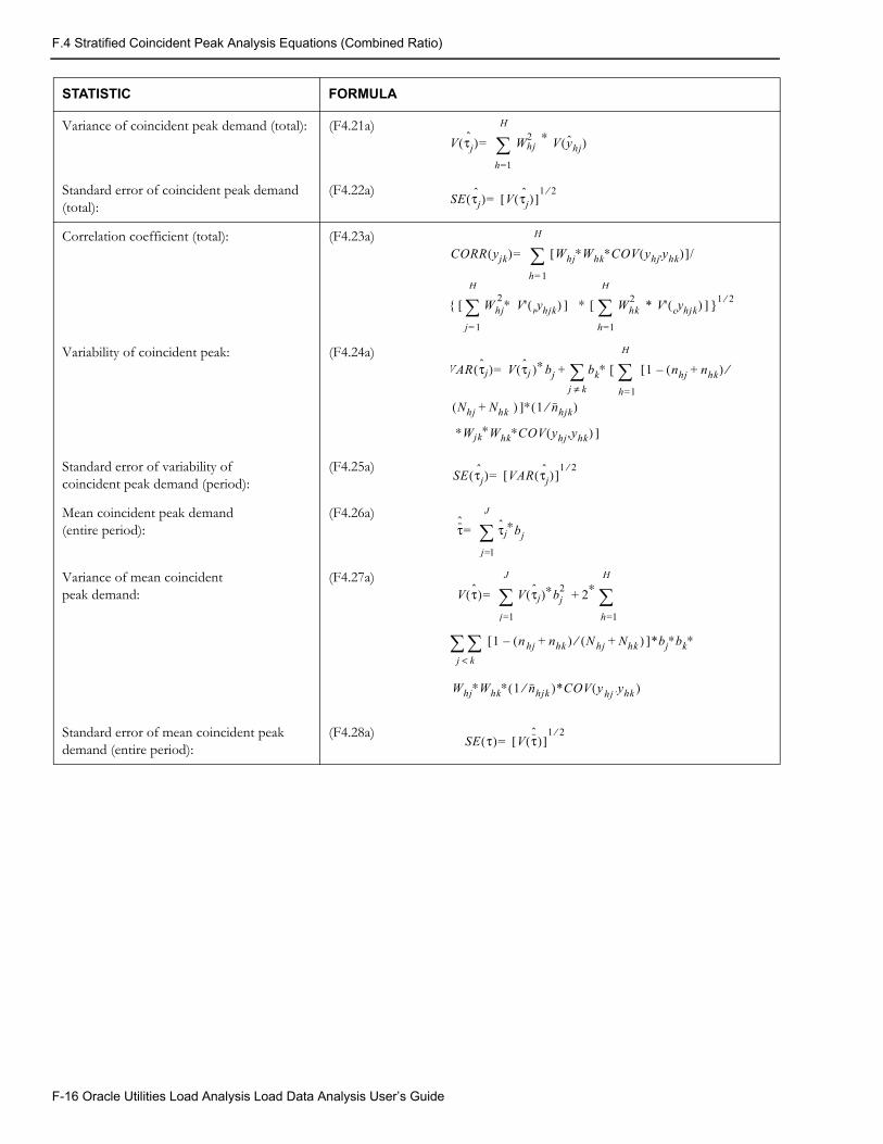
F.4 Stratified Coincident Peak Analysis Equations (Combined Ratio)
Variance of coincident peak demand (total): (F4.21a)
Standard error of coincident peak demand (total):
(F4.22a)
Correlation coefficient (total): (F4.23a)
Variability of coincident peak: (F4.24a)
Standard error of variability of coincident peak demand (period):
(F4.25a)
Mean coincident peak demand (entire period):
(F4.26a)
Variance of mean coincident peak demand:
(F4.27a)
Standard error of mean coincident peak demand (entire period):
(F4.28a)
STATISTIC FORMULA
V τjˆ( ) W2
hj∗ V yhj( )
h 1=
H
=
SE τjˆ( ) V τj
ˆ( )[ ]1 2⁄
=
CORR yjk( ) Whj∗Whk∗COV yhj'yhk( )[ ]/h 1=
H
=
{ [ Whj∗2 V' yr hjk( ) ] ∗ [ Whk
2 * V' yc hjk( ) ] }1 2⁄
h 1=
H
j 1=
H
VAR τj( ) V τj )∗( bj bk∗ [ h 1=
H
j k≠+= 1[ nhj nhk+( ) ⁄–
Nhj Nhk+ ( ) ]∗ 1 nhjk⁄( )
∗Wjk∗Whk∗COV yhj,yhk( ) ]
SE τjˆ( ) VAR τj
ˆ( )[ ]1 2⁄
=
τˆ
τj∗bjj 1=
J
=
V τ( ) V τj( )∗bj2 2+ ∗
h 1=
H
j 1=
J
=
j k< 1[ n( hj nhk )+ N( hj Nhk ) ]+⁄– *bj∗bk∗
Whj∗Whk∗ 1 nhjk )*⁄ COV y( hj ,yhk )(
SE τ( ) V τˆ
( )[ ]1 2⁄
=
F-16 Oracle Utilities Load Analysis Load Data Analysis User’s Guide
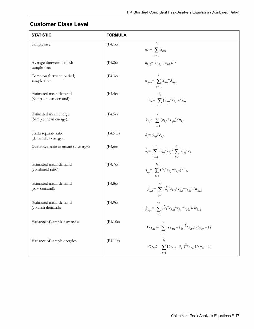
F.4 Stratified Coincident Peak Analysis Equations (Combined Ratio)
Customer Class Level
STATISTIC FORMULA
Sample size: (F4.1c)
Average (between period) sample size:
(F4.2c)
Common (between period) sample size:
(F4.3c)
Estimated mean demand(Sample mean demand):
(F4.4c)
Estimated mean energy (Sample mean energy):
(F4.5c)
Strata separate ratio (demand to energy):
(F4.51c)
Combined ratio (demand to energy): (F4.6c)
Estimated mean demand (combined ratio):
(F4.7c)
Estimated mean demand (row demand):
(F4.8c)
Estimated mean demand (column demand):
(F4.9c)
Variance of sample demands: (F4.10c)
Variance of sample energies: (F4.11c)
nhj Xhjii 1=
Ih
=
nhjk nhj nhk+( ) 2⁄=
n'hjk Xhji∗Xhkii 1=
I
=
yhj yhji∗xhji( ) nhj⁄i 1=
Ih
=
ehj ehji∗xhji( ) nhj⁄i 1=
Ih
=
Rjˆ yhj ehj⁄=
Rj Whj∗yhj Whj∗ehjh 1=
H
⁄h 1=
H
=
y hj Rj∗ehji∗xhji( ) nhj⁄i 1=
Ih
=
yr hjk Rj∗ehji∗xhji∗xhki( ) n'hjk⁄i 1=
Ih
=
yc hjk Rk∗ehki∗xhji∗xhki( ) n'hjk⁄i 1=
Ih
=
V yhj( ) yhji yhj–( )2*xhji[ ] nhj 1–( )⁄i 1=
Ih
=
V ehj( ) ehji ehj–( )2*xhji[ ] nhj 1–( )⁄
i 1=
Ih
=
Coincident Peak Analysis Equations F-17
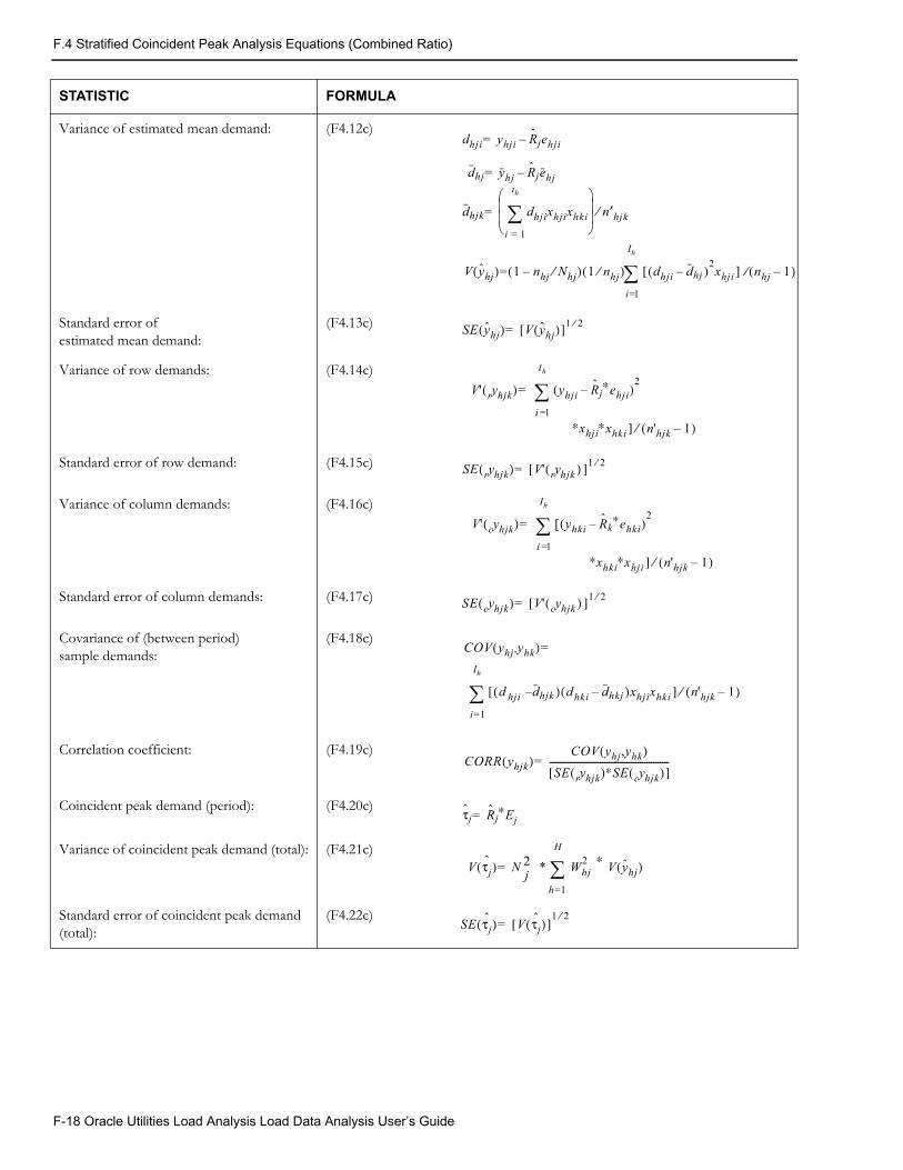
F.4 Stratified Coincident Peak Analysis Equations (Combined Ratio)
Variance of estimated mean demand: (F4.12c)
Standard error ofestimated mean demand:
(F4.13c)
Variance of row demands: (F4.14c)
Standard error of row demand: (F4.15c)
Variance of column demands: (F4.16c)
Standard error of column demands: (F4.17c)
Covariance of (between period) sample demands:
(F4.18c)
Correlation coefficient: (F4.19c)
Coincident peak demand (period): (F4.20c)
Variance of coincident peak demand (total): (F4.21c)
Standard error of coincident peak demand (total):
(F4.22c)
STATISTIC FORMULA
dhji yhji Rjehji–=
dhj yhj Rjehj–=
dhjk dhjixhjixhkii 1=
ih
n′hjk⁄=
V yhj( ) 1 nhj Nhj⁄–( ) 1 nhj⁄( ) dhji dhj )2xhji ]–([ nhj 1–( )⁄
i 1=
Ih
=
SE yhj( ) V yhj( )[ ]1 2⁄=
V' yr hjk( ) yhji Rj∗ehji–( )2
i 1=
Ih
=
∗xhji∗xhki ] n'hjk 1–( )⁄
SE yr hjk( ) V' yr hjk )([ ]1 2⁄=
V' yc hjk( ) [ yhki Rk∗ehki–( )2
i 1=
Ih
=
∗xhki∗xhji ] n'hjk 1–( )⁄
SE yc hjk( ) V' yc hjk )([ ]1 2⁄=
COV yhj ,yhk( )=
d([ hji dhjk ) d( hki dhkj )– xhjixhki ] n'hjk 1–( )⁄–i 1=
Ih
CORR yhjk( )COV yhj,yhk( )
SE yr hjk( )∗SE yc hjk( )[ ]------------------------------------------------------=
τj Rj∗Ej=
V τjˆ( ) N 2
j * Whj2 ∗ V yhj( )
h 1=
H
=
SE τjˆ( ) V τj
ˆ( )[ ]1 2⁄
=
F-18 Oracle Utilities Load Analysis Load Data Analysis User’s Guide
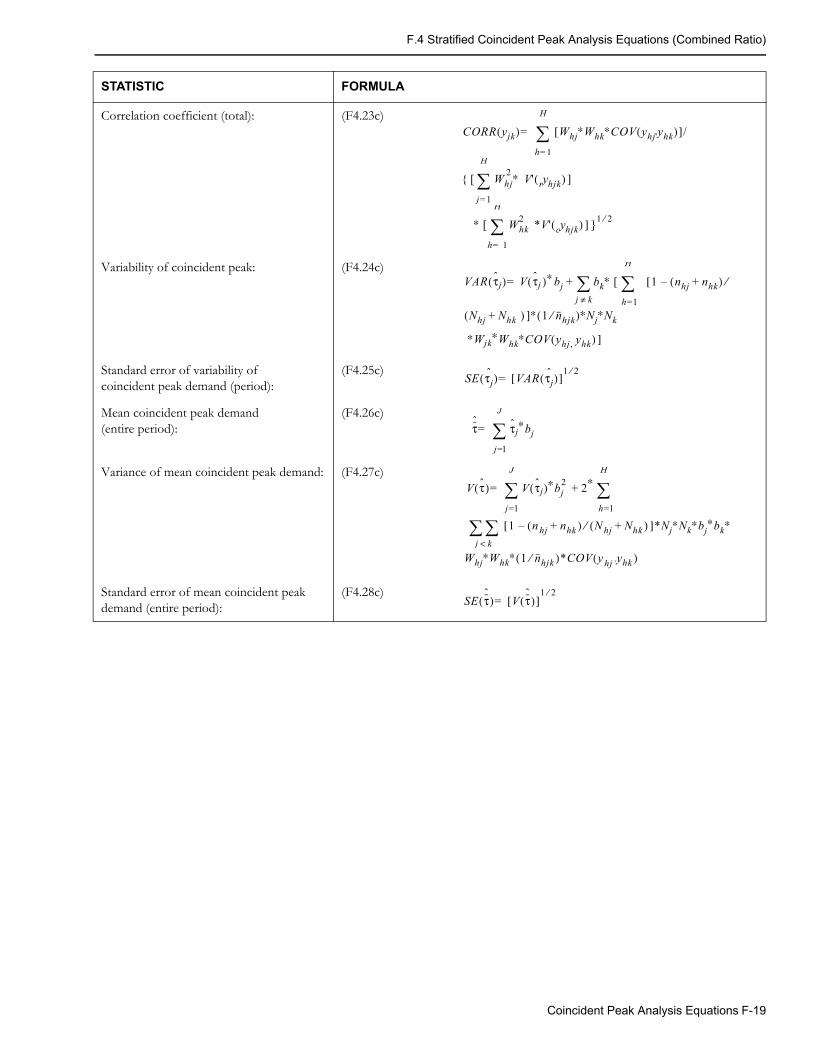
F.4 Stratified Coincident Peak Analysis Equations (Combined Ratio)
Correlation coefficient (total): (F4.23c)
Variability of coincident peak: (F4.24c)
Standard error of variability of coincident peak demand (period):
(F4.25c)
Mean coincident peak demand (entire period):
(F4.26c)
Variance of mean coincident peak demand: (F4.27c)
Standard error of mean coincident peak demand (entire period):
(F4.28c)
STATISTIC FORMULA
CORR yjk( ) Whj∗Whk∗COV yhj'yhk( )[ ]/h 1=
H
=
{ [ Whj∗2 V' yr hjk( ) ]
j 1=
H
∗ [ Whk2 *V' yc hjk( ) ] }1 2⁄
h 1=
H
VAR τj( ) V τj )∗( bj bk∗ [ h 1=
H
j k≠+= 1[ nhj nhk+( ) ⁄–
Nhj Nhk+ ( ) ]∗ 1 nhjk⁄( )∗Nj∗Nk
∗Wjk∗Whk∗COV yhj , yhk( ) ]
SE τjˆ( ) VAR τj
ˆ( )[ ]1 2⁄
=
τˆ
τj∗bjj 1=
J
=
V τ( ) V τj( )∗bj2 2+ ∗
h 1=
H
j 1=
J
=
j k< 1[ n( hj nhk )+ N( hj Nhk ) ]+⁄– *Nj∗Nk∗bj∗bk∗
Whj∗Whk∗ 1 nhjk )⁄ *COV y( hj ,yhk )(
SE τˆ
( ) V τˆ
( )[ ]1 2⁄
=
Coincident Peak Analysis Equations F-19

F.4 Stratified Coincident Peak Analysis Equations (Combined Ratio)
F-20 Oracle Utilities Load Analysis Load Data Analysis User’s Guide
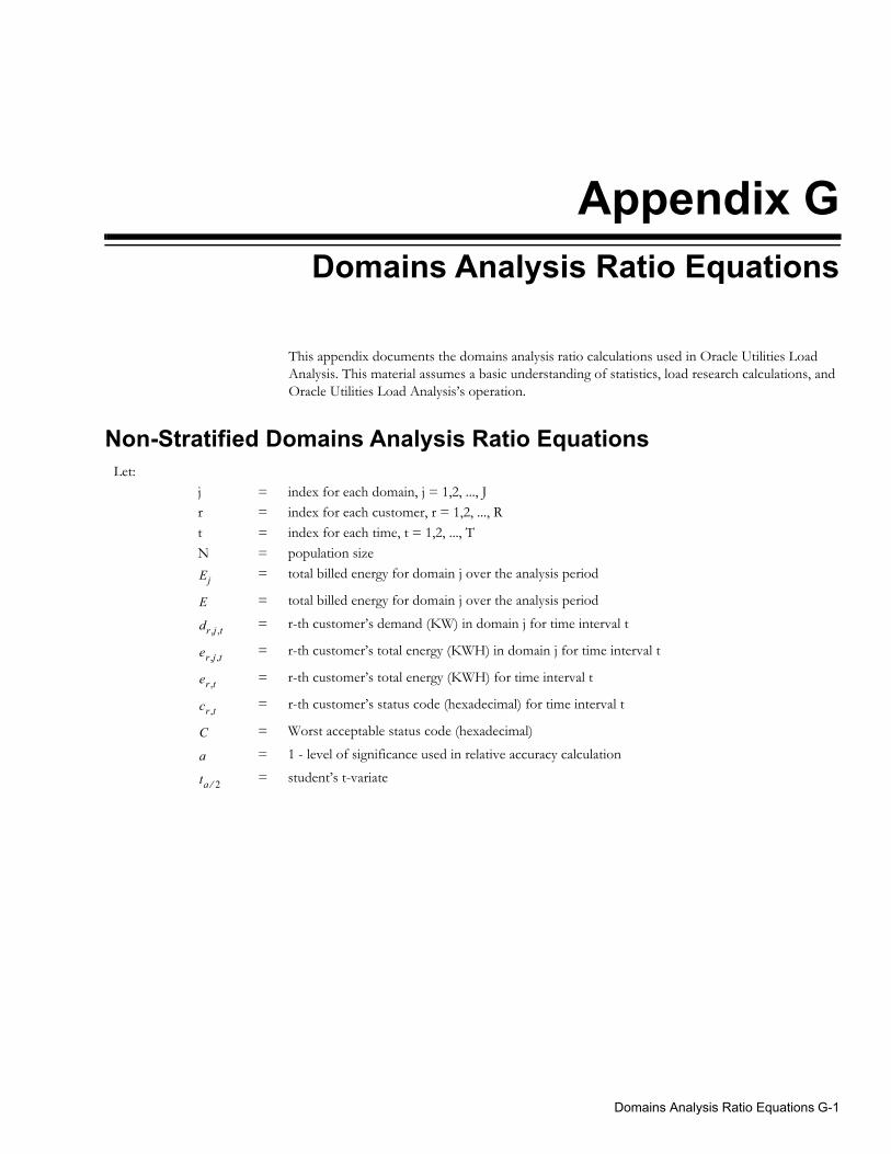
Appendix GDomains Analysis Ratio Equations
This appendix documents the domains analysis ratio calculations used in Oracle Utilities Load Analysis. This material assumes a basic understanding of statistics, load research calculations, and Oracle Utilities Load Analysis’s operation.
Non-Stratified Domains Analysis Ratio EquationsLet:
j = index for each domain, j = 1,2, ..., Jr = index for each customer, r = 1,2, ..., Rt = index for each time, t = 1,2, ..., T
N = population size= total billed energy for domain j over the analysis period
= total billed energy for domain j over the analysis period
= r-th customer’s demand (KW) in domain j for time interval t
= r-th customer’s total energy (KWH) in domain j for time interval t
= r-th customer’s total energy (KWH) for time interval t
= r-th customer’s status code (hexadecimal) for time interval t
= Worst acceptable status code (hexadecimal)
= 1 - level of significance used in relative accuracy calculation
= student’s t-variate
Ej
E
dr j t,,
er j t,,
er t,
cr t,
C
a
ta 2⁄
Domains Analysis Ratio Equations G-1
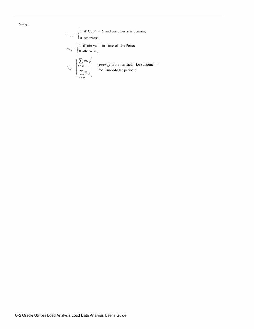
Define:
xr j t, , = 1 if Cr t, < C and customer is in domain; =
0 otherwise
mt p, = 1 if interval is in Time-of-Use Period0 otherwise t
fr p, =
mt p,t p∈
xr t,t p∈
--------------------
(energy proration factor for customer r for Time-of-Use period p)
G-2 Oracle Utilities Load Analysis Load Data Analysis User’s Guide
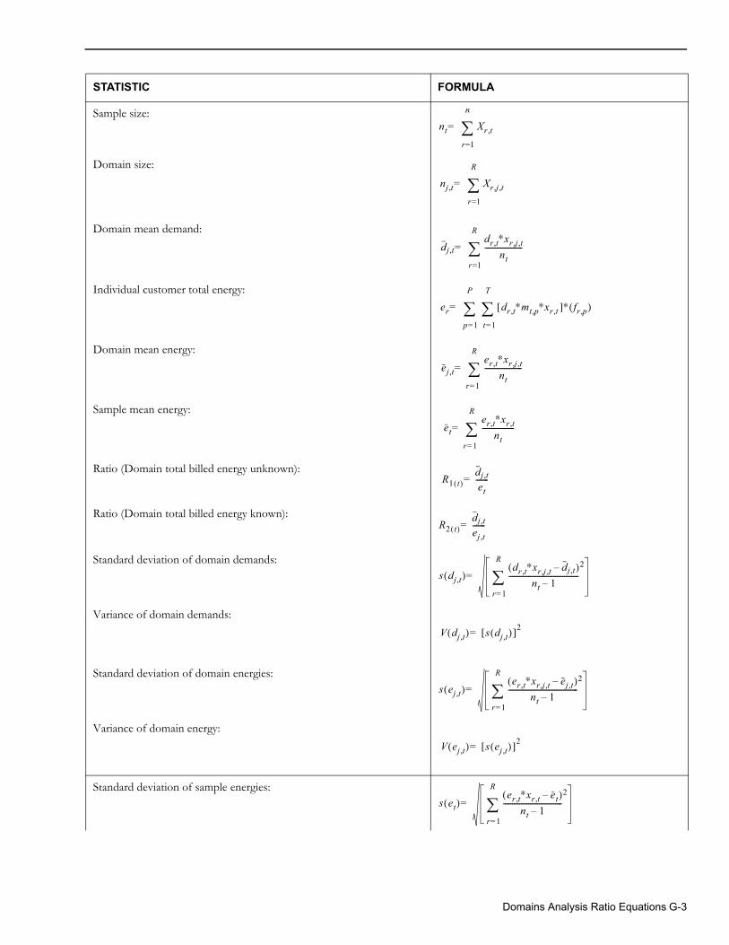
STATISTIC FORMULA
Sample size:
Domain size:
Domain mean demand:
Individual customer total energy:
Domain mean energy:
Sample mean energy:
Ratio (Domain total billed energy unknown):
Ratio (Domain total billed energy known):
Standard deviation of domain demands:
Variance of domain demands:
Standard deviation of domain energies:
Variance of domain energy:
Standard deviation of sample energies:
nt Xr t,r 1=
R
=
nj t, Xr j t,,
r 1=
R
=
dj t,dr t, ∗xr j t,,nt
---------------------r 1=
R
=
er dr t, ∗mt p, ∗xr t, ]∗ fr p,( )[t 1=
T
p 1=
P
=
ej t,er t, ∗xr j t,,nt
---------------------r 1=
R
=
eter t, ∗xr t,nt
------------------r 1=
R
=
R1 t( )dj t,et
-------=
R2 t( )dj t,ej t,-------=
s dj t,( )dr t, ∗xr j t,, dj t,–( )
nt 1–---------------------------------------
2
r 1=
R
=
V dj t,( ) s dj t,( )[ ]2=
s ej t,( )er t, ∗xr j t,, ej t,–( )
nt 1–---------------------------------------
2
r 1=
R
=
V ej t,( ) s ej t,( )[ ]2=
s et( )er t, ∗xr t, et–( )nt 1–
---------------------------------2
r 1=
R
=
Domains Analysis Ratio Equations G-3
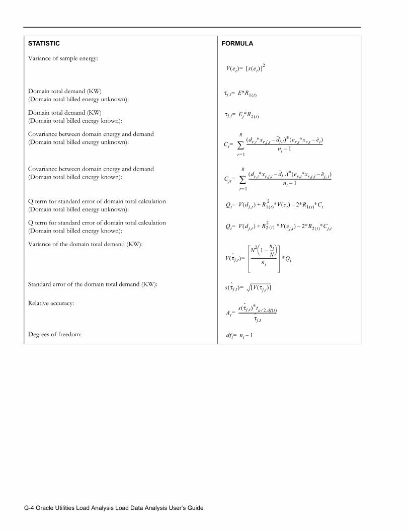
Variance of sample energy:
Domain total demand (KW) (Domain total billed energy unknown):
Domain total demand (KW) (Domain total billed energy known):
Covariance between domain energy and demand(Domain total billed energy unknown):
Covariance between domain energy and demand (Domain total billed energy known):
Q term for standard error of domain total calculation (Domain total billed energy unknown):
Q term for standard error of domain total calculation (Domain total billed energy known):
Variance of the domain total demand (KW):
Standard error of the domain total demand (KW):
Relative accuracy:
Degrees of freedom:
STATISTIC FORMULA
V et( ) s et( )[ ]2=
τj t, E∗R1 t( )=
τj t, Ej∗R2 t( )=
Ctdr t, ∗xr j t,, dj t,–( )∗ er t, ∗xr t, et–( )
nt 1–----------------------------------------------------------------------------
r 1=
R
=
Cjtdr t, ∗xr j t,, dj t,–( )∗ er t, ∗xr j t,, ej t,–( )
nt 1–-----------------------------------------------------------------------------------
r 1=
R
=
Qt V d( j t, ) R1 t( )∗V et( ) 2∗R1 t( )∗Ct–2+=
Qt V d( j t, ) R22 t( ) *V ej t,( ) 2∗R2 t( )∗Cj t,–+=
V τj t,( )N2 1
ntN----–
nt-------------------------- ∗Qt=
s τj t,( ) V τj t,( )[ ]=
Ats τj t,( )∗ta 2 df t( ),⁄
τj t,--------------------------------------=
dft nt 1–=
G-4 Oracle Utilities Load Analysis Load Data Analysis User’s Guide
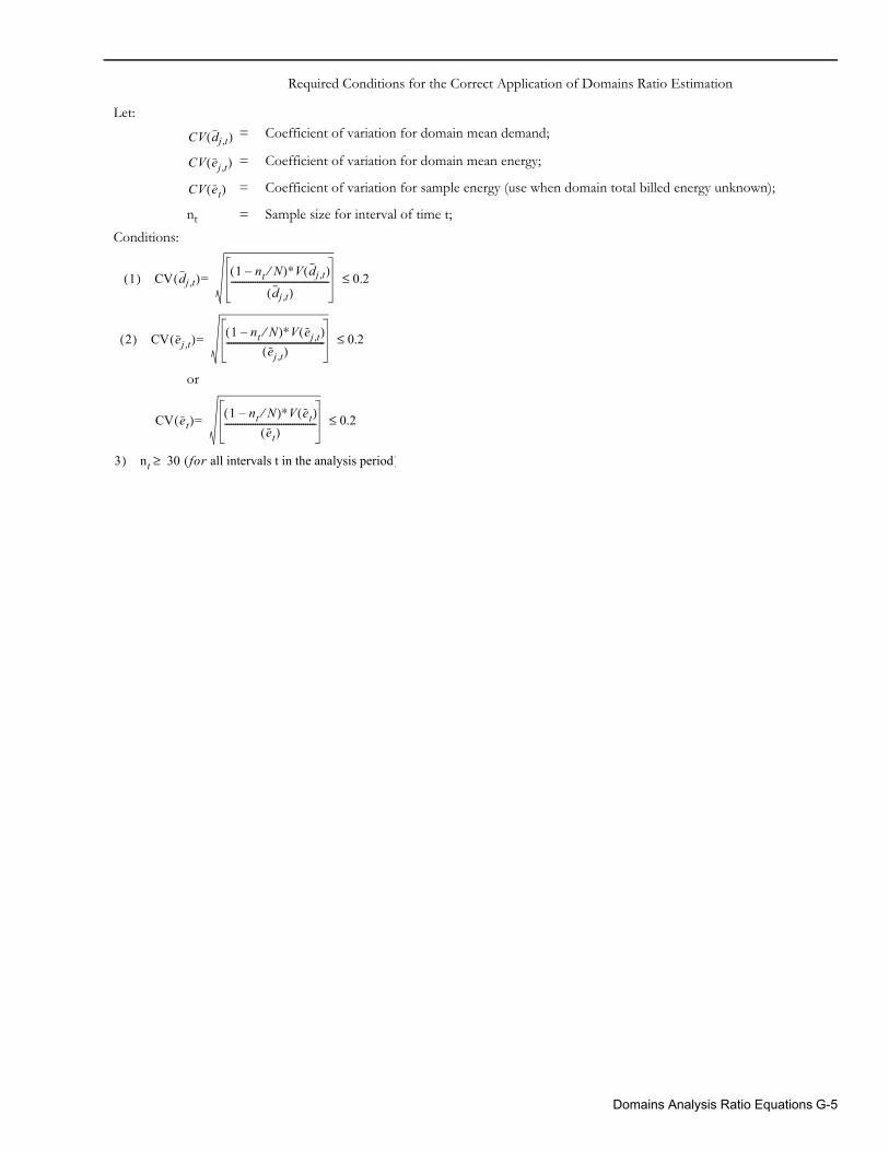
Required Conditions for the Correct Application of Domains Ratio Estimation
Let:
= Coefficient of variation for domain mean demand;
= Coefficient of variation for domain mean energy;
= Coefficient of variation for sample energy (use when domain total billed energy unknown);
nt = Sample size for interval of time t;
Conditions:
or
CV dj t,( )
CV ej t,( )
CV et( )
1( ) CV dj t,( ) 1 nt N⁄–( )∗V dj t,( )
dj t,( )--------------------------------------------- 0.2≤=
2( ) CV ej t,( ) 1 nt N⁄–( )∗V ej t,( )ej t,( )
--------------------------------------------- 0.2≤=
CV et( ) 1 nt N⁄–( )∗V et( )et( )
------------------------------------------ 0.2≤=
3) nt 30 for all intervals t in the analysis period( )≥
Domains Analysis Ratio Equations G-5
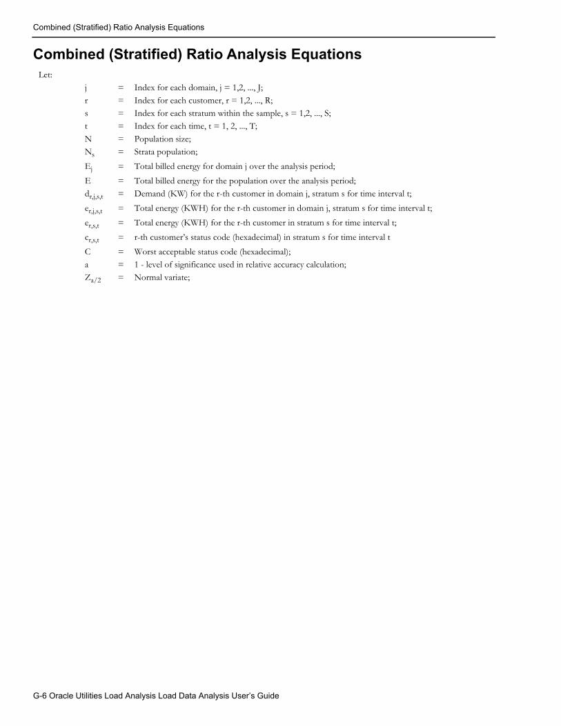
Combined (Stratified) Ratio Analysis Equations
Combined (Stratified) Ratio Analysis EquationsLet:
j = Index for each domain, j = 1,2, ..., J;
r = Index for each customer, r = 1,2, ..., R;s = Index for each stratum within the sample, s = 1,2, ..., S;t = Index for each time, t = 1, 2, ..., T;
N = Population size;Ns = Strata population;
Ej = Total billed energy for domain j over the analysis period;
E = Total billed energy for the population over the analysis period;dr,j,s,t = Demand (KW) for the r-th customer in domain j, stratum s for time interval t;
er,j,s,t = Total energy (KWH) for the r-th customer in domain j, stratum s for time interval t;
er,s,t = Total energy (KWH) for the r-th customer in stratum s for time interval t;
cr,s,t = r-th customer’s status code (hexadecimal) in stratum s for time interval t
C = Worst acceptable status code (hexadecimal);a = 1 - level of significance used in relative accuracy calculation;Za/2 = Normal variate;
G-6 Oracle Utilities Load Analysis Load Data Analysis User’s Guide
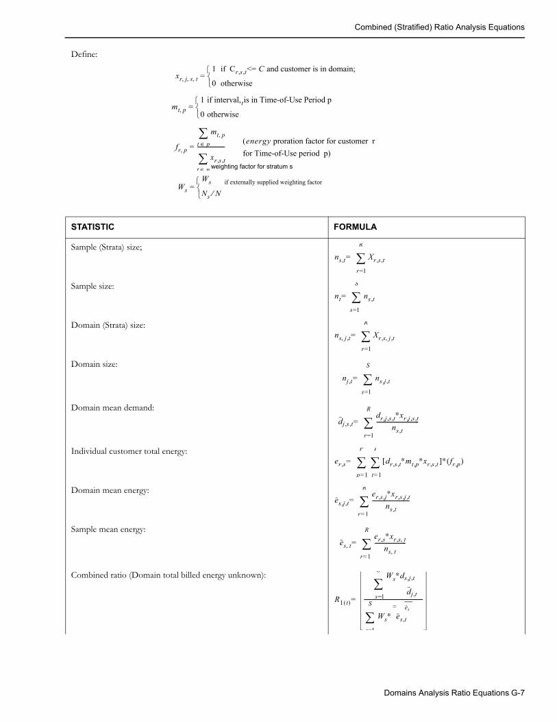
Combined (Stratified) Ratio Analysis Equations
Define:
xr j s t, , , = 1 if Cr s t,, <= C and customer is in domain;
0 otherwise
mt p, = 1 if interval,tis in Time-of-Use Period p
0 otherwise
fr p, =
mt p,t p∈
xr s t,,t p∈--------------------
(energy proration factor for customer r for Time-of-Use period p)
weighting factor for stratum s
Ws = Ws if externally supplied weighting factor
Ns N⁄
STATISTIC FORMULA
Sample (Strata) size;
Sample size:
Domain (Strata) size:
Domain size:
Domain mean demand:
Individual customer total energy:
Domain mean energy:
Sample mean energy:
Combined ratio (Domain total billed energy unknown):
ns t, Xr s t,,r 1=
R
=
nt ns t,s 1=
S
=
ns j t,, Xr s j t,,,
r 1=
R
=
nj t, ns j t,,
s 1=
S
=
dj s t,,dr j s t,,, ∗xr j s t,,,
ns t,-------------------------------
r 1=
R
=
er s, dr s t,, ∗mt p, ∗xr s t,, ]∗ fr p,( )[t 1=
T
p 1=
P
=
es j, t,er s j,, ∗xr s j t,,,
ns t,---------------------------
r 1=
R
=
es t,er s, ∗xr s t,,ns t,
-----------------------r 1=
R
=
R1 t( )
Ws∗ds j t,,
dj t,s 1=
S
Ws∗ es t, et=
s 1=
S
-------------------------------------------=
Domains Analysis Ratio Equations G-7
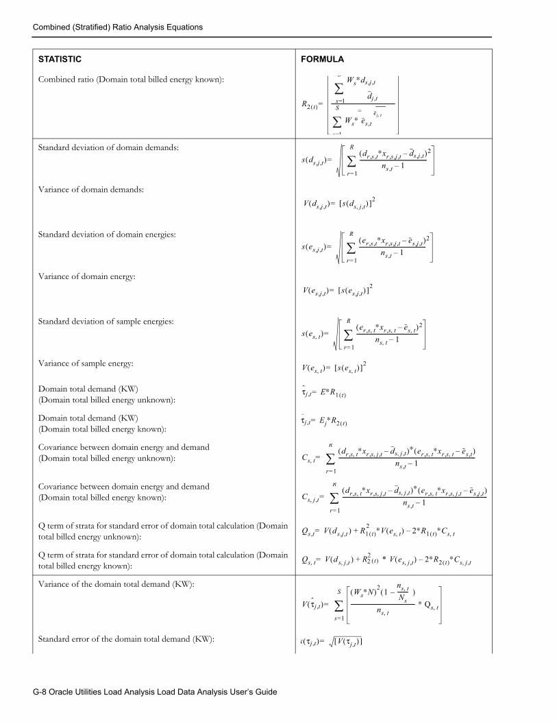
Combined (Stratified) Ratio Analysis Equations
Combined ratio (Domain total billed energy known):
Standard deviation of domain demands:
Variance of domain demands:
Standard deviation of domain energies:
Variance of domain energy:
Standard deviation of sample energies:
Variance of sample energy:
Domain total demand (KW)(Domain total billed energy unknown):
Domain total demand (KW)(Domain total billed energy known):
Covariance between domain energy and demand(Domain total billed energy unknown):
Covariance between domain energy and demand (Domain total billed energy known):
Q term of strata for standard error of domain total calculation (Domain total billed energy unknown):
Q term of strata for standard error of domain total calculation (Domain total billed energy known):
Variance of the domain total demand (KW):
Standard error of the domain total demand (KW):
STATISTIC FORMULA
R2 t( )
Ws∗ds j t,,
dj t,s 1=
S
Ws∗ es t, ej t,=
s 1=
S
-----------------------------------------------=
s ds j, t,( )dr s t,, ∗xr s j, t,, ds j, t,–( )
ns t, 1–-------------------------------------------------
2
r 1=
R
=
V ds j, t,( ) s ds j t,,( )[ ]2=
s es j, t,( )er s t,, ∗xr s j, t,, es j, t,–( )
ns t, 1–-------------------------------------------------
2
r 1=
R
=
V es j, t,( ) s es j, t,( )[ ]2=
s es t,( )er s t,, ∗xr s t,, es t,–( )
ns t, 1–---------------------------------------------
2
r 1=
R
=
V es t,( ) s es t,( )[ ]2=
τj t, E∗R1 t( )=
τj t, Ej∗R2 t( )=
Cs t,dr s t,, ∗xr s j t,,, ds j t,,–( )∗ er s t,, ∗xr s t,, es t,–( )
ns t, 1–----------------------------------------------------------------------------------------------------
r 1=
R
=
Cs j t,,dr s t,, ∗xr s j t,,, ds j t,,–( )∗ er s t,, ∗xr s j t,,, es j t,,–( )
ns t, 1–----------------------------------------------------------------------------------------------------------
r 1=
R
=
Qs t, V d( s j, t, ) R1 t( )∗V es t,( ) 2∗R1 t( )∗Cs t,–2+=
Qs t, V d( s j t,, ) R22 t( ) * V es j t,,( ) 2∗R2 t( )∗Cs j t,,–+=
V τj t,( )Ws∗N( )2 1(
ns t,Ns-------- )–
ns t,----------------------------------------------- ∗ Qs t,
s 1=
S
=
s τj t,( ) V τj t,( )[ ]=
G-8 Oracle Utilities Load Analysis Load Data Analysis User’s Guide

Combined (Stratified) Ratio Analysis Equations
Relative accuracy:
STATISTIC FORMULA
Ats τj t,( )∗Za 2 df t( ),⁄
τj t,----------------------------------------=
Domains Analysis Ratio Equations G-9
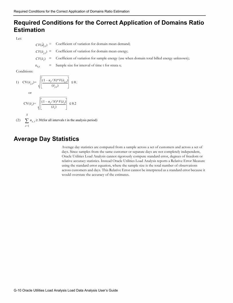
Required Conditions for the Correct Application of Domains Ratio Estimation
Required Conditions for the Correct Application of Domains Ratio Estimation
Average Day StatisticsAverage day statistics are computed from a sample across a set of customers and across a set of days. Since samples from the same customer or separate days are not completely independent, Oracle Utilities Load Analysis cannot rigorously compute standard error, degrees of freedom or relative accuracy statistics. Instead Oracle Utilities Load Analysis reports a Relative Error Measure using the standard error equation, where the sample size is the total number of observations across customers and days. This Relative Error cannot be interpreted as a standard error because it would overstate the accuracy of the estimates.
Let:= Coefficient of variation for domain mean demand;
= Coefficient of variation for domain mean energy;
= Coefficient of variation for sample energy (use when domain total billed energy unknown);
ns,t = Sample size for interval of time t for strata s;
Conditions:
or
CV dj t,( )
CV ej t,( )
CV et( )
1) CV ej t,( ) 1 nt N⁄–( )∗V ej t,( )ej t,( )
--------------------------------------------- 0.2≤=
CV et( ) 1 nt N⁄–( )∗V et( )et( )
------------------------------------------ 0.2≤=
2( ) ns t, 30(for all intervals t in the analysis period)≥s 1=
S
G-10 Oracle Utilities Load Analysis Load Data Analysis User’s Guide
Appendix HDomains Analysis Mean Per Unit Equations
This appendix documents the domains analysis mean per unit calculations used in Oracle Utilities Load Analysis. This material assumes a basic understanding of statistics load research calculations, and Oracle Utilities Load Analysis’s operation.
Domains Analysis Mean Per Unit Equations H-1
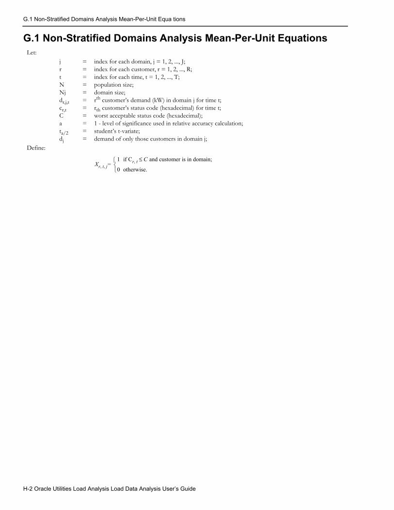
G.1 Non-Stratified Domains Analysis Mean-Per-Unit Equa tions
G.1 Non-Stratified Domains Analysis Mean-Per-Unit EquationsLet:
jrtNNjdr,j,tcr,tCata/2dj
===========
index for each domain, j = 1, 2, ..., J;index for each customer, r = 1, 2, ..., R;index for each time, t = 1, 2, ..., T;population size;domain size;rth customer’s demand (kW) in domain j for time t;rth customer’s status code (hexadecimal) for time t;worst acceptable status code (hexadecimal);1 - level of significance used in relative accuracy calculation;student’s t-variate;demand of only those customers in domain j;
Define:
Xr t j, ,1 if Cr t, C and customer is in domain;≤
0 otherwise.
=
H-2 Oracle Utilities Load Analysis Load Data Analysis User’s Guide
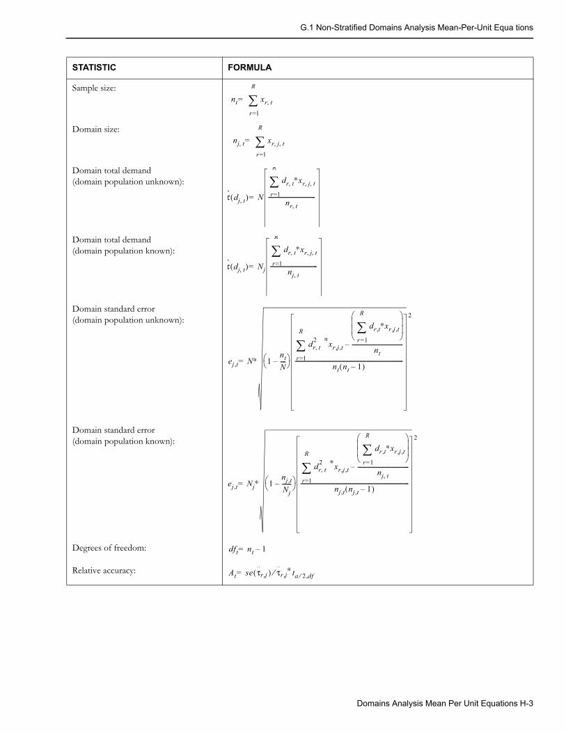
G.1 Non-Stratified Domains Analysis Mean-Per-Unit Equa tions
STATISTIC FORMULA
Sample size:
Domain size:
Domain total demand(domain population unknown):
Domain total demand(domain population known):
Domain standard error(domain population unknown):
Domain standard error(domain population known):
Degrees of freedom:
Relative accuracy:
nt xr t,r 1=
R
=
nj t, xr j t, ,
r 1=
R
=
τ dj t,( ) N
dr t, ∗xr j t, ,
r 1=
R
nr t,
----------------------------------=
τ dj t,( ) Nj
dr t, ∗xr j t, ,
r 1=
R
nj t,
----------------------------------=
ej t, N∗ 1ntN----–
dr t,2 ∗xr j t,,
dr t, ∗xr j t,,
r 1=
R
nt-------------------------------------–
r 1=
R
nt nt 1–( )
------------------------------------------------------------------------------
2
=
ej t, Nj∗ 1nj t,Nj-------–
dr t,2 ∗xr j t,,
dr t, ∗xr j t,,
r 1=
R
nj t,-------------------------------------–
r 1=
R
nj t, nj t, 1–( )
------------------------------------------------------------------------------
2
=
dft nt 1–=
At se τr j, ) τr j,⁄ ∗( ta 2 df,⁄=
Domains Analysis Mean Per Unit Equations H-3
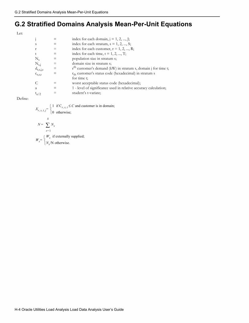
G.2 Stratified Domains Analysis Mean-Per-Unit Equations
G.2 Stratified Domains Analysis Mean-Per-Unit EquationsLet:
jsrtNsNs,jdr,s,j,tcr,s,t
Cata/2
========
===
index for each domain, j = 1, 2, ..., J;index for each stratum, s = 1, 2, ..., S;index for each customer, r = 1, 2, ..., R;index for each time, t = 1, 2, ..., T;population size in stratum s;domain size in stratum s;rth customer’s demand (kW) in stratum s, domain j for time t;rth customer’s status code (hexadecimal) in stratum sfor time t;worst acceptable status code (hexadecimal);1 - level of significance used in relative accuracy calculation;student’s t-variate;
Define:
Xr s t j, , ,1 if Cr s t, , C and customer is in domain;≤
0 otherwise;
=
N Nss 1=
S
=
WsWs if externally supplied;
Ns/N otherwise.
=
H-4 Oracle Utilities Load Analysis Load Data Analysis User’s Guide
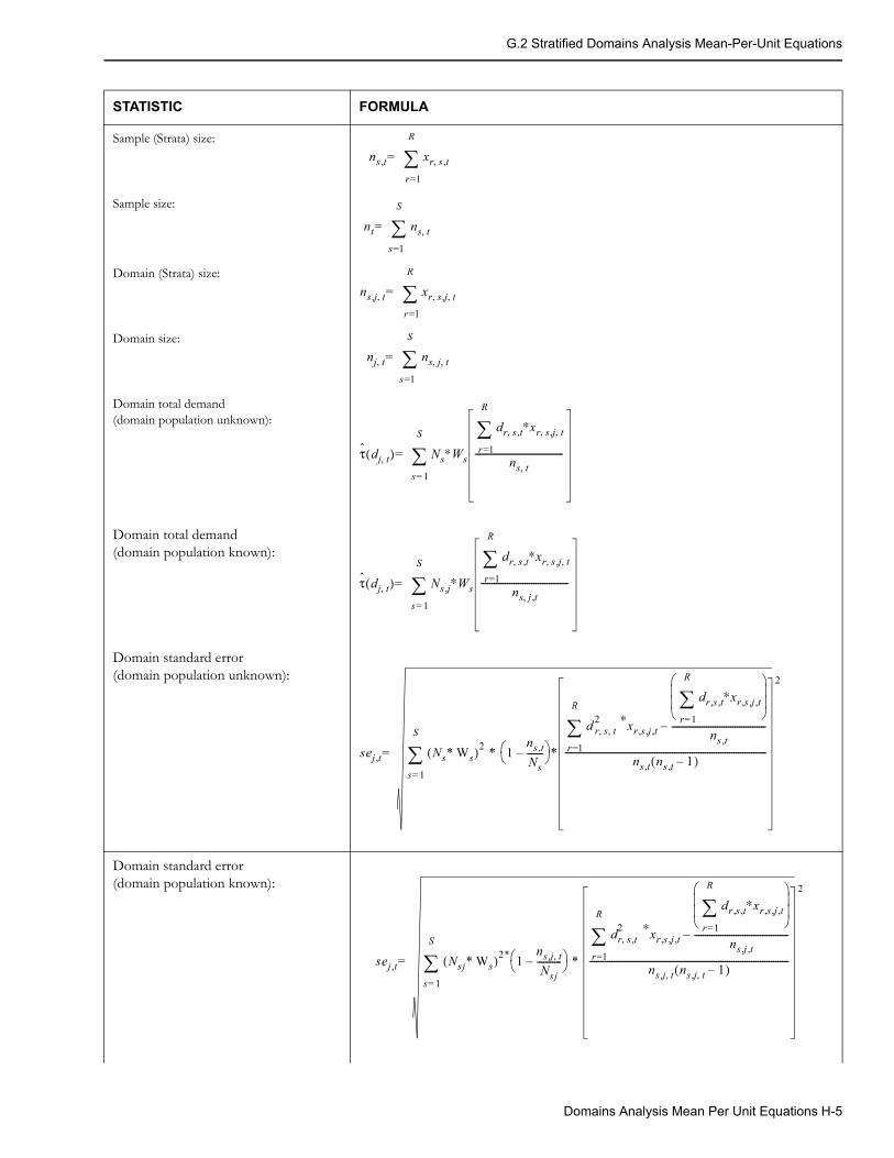
G.2 Stratified Domains Analysis Mean-Per-Unit Equations
STATISTIC FORMULA
Sample (Strata) size:
Sample size:
Domain (Strata) size:
Domain size:
Domain total demand(domain population unknown):
Domain total demand(domain population known):
Domain standard error(domain population unknown):
Domain standard error(domain population known):
ns t, xr s t,,
r 1=
R
=
nt ns t,s 1=
S
=
ns j, t, xr s j, t, ,
r 1=
R
=
nj t, ns j t, ,
s 1=
S
=
τ dj t,( ) Ns∗Wss 1=
S
dr s t,, ∗xr s j, t, ,
r 1=
R
ns t,
----------------------------------------=
τ dj t,( ) Ns j, ∗Wss 1=
S
dr s t,, ∗xr s j, t, ,
r 1=
R
ns j t,,
----------------------------------------=
sej t, Ns* Ws( )2 * 1ns t,Ns-------–
*s 1=
S
d r s t, ,2 ∗xr s j, t,,
dr s t,, ∗xr s j, t,,
r 1=
R
ns t,-------------------------------------------–
r 1=
R
ns t, ns t, 1–( )
--------------------------------------------------------------------------------------------
2
=
sej t, Nsj* Ws( )2* 1ns j t,,Nsj
-----------– *
s 1=
S
dr s t,,2 ∗xr s j, t,,
dr s t,, ∗xr s j, t,,
r 1=
R
ns j t,,-------------------------------------------–
r 1=
R
ns j t,, ns j t,, 1–( )
-------------------------------------------------------------------------------------------
2
=
Domains Analysis Mean Per Unit Equations H-5
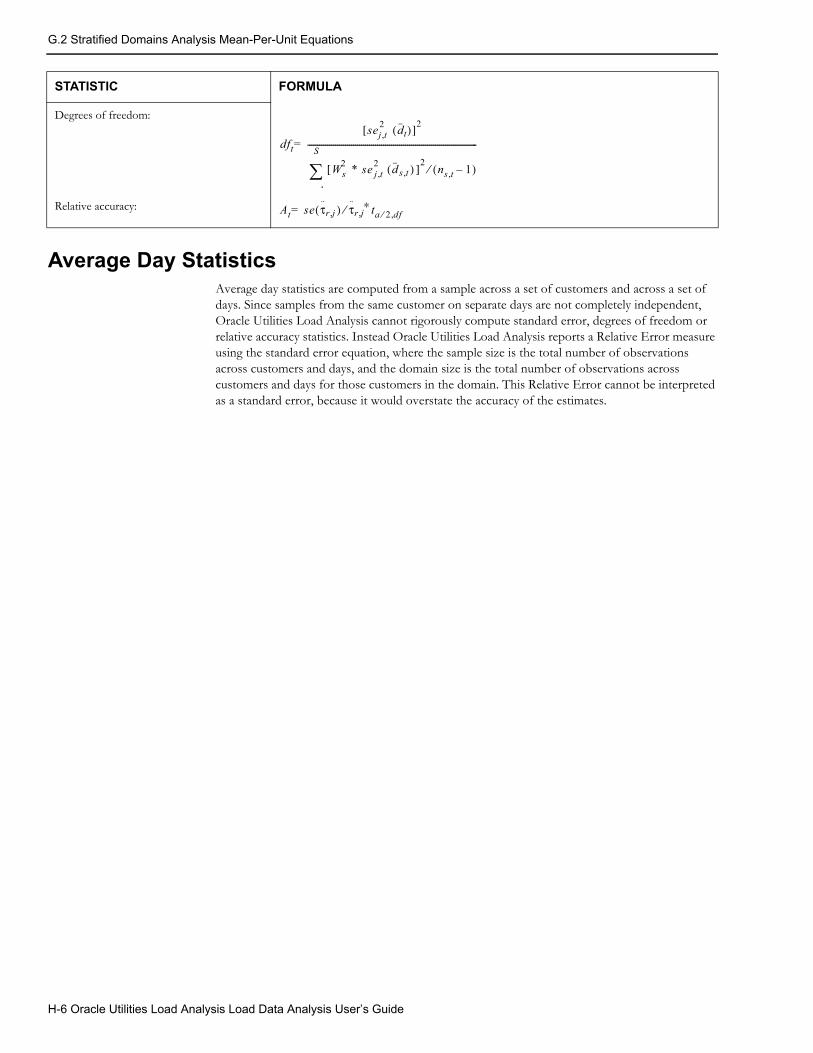
G.2 Stratified Domains Analysis Mean-Per-Unit Equations
Average Day StatisticsAverage day statistics are computed from a sample across a set of customers and across a set of days. Since samples from the same customer on separate days are not completely independent, Oracle Utilities Load Analysis cannot rigorously compute standard error, degrees of freedom or relative accuracy statistics. Instead Oracle Utilities Load Analysis reports a Relative Error measure using the standard error equation, where the sample size is the total number of observations across customers and days, and the domain size is the total number of observations across customers and days for those customers in the domain. This Relative Error cannot be interpreted as a standard error, because it would overstate the accuracy of the estimates.
Degrees of freedom:
Relative accuracy:
STATISTIC FORMULA
dftsej t,
2 dt( )[ ]2
Ws2 * se j t,
2 d( s t, ) ]2 ns t, 1–( )⁄[
1
S
-------------------------------------------------------------------------------------=
At se τr j, ) τr j,⁄ ∗( ta 2 df,⁄=
H-6 Oracle Utilities Load Analysis Load Data Analysis User’s Guide

Appendix IDomains Analysis Ratio Equations
This appendix documents the domains analysis ratio calculations used in Oracle Utilities Load Analysis. This material assumes a basic understanding of statistics, load research calculations, and Oracle Utilities Load Analysis’s operation.
H.1 Non-Stratified Domains Analysis Ratio EquationsLet:
j = index for each domain, j = 1,2, ..., Jr = index for each customer, r = 1,2, ..., Rt = index for each time, t = 1,2, ..., T
N = population size= total billed energy for domain j over the analysis period
= total billed energy for domain j over the analysis period
= r-th customer’s demand (KW) in domain j for time interval t
= r-th customer’s total energy (KWH) in domain j for time interval t
= r-th customer’s total energy (KWH) for time interval t
= r-th customer’s status code (hexadecimal) for time interval t
= Worst acceptable status code (hexadecimal)
= 1 - level of significance used in relative accuracy calculation
= student’s t-variate
Ej
E
dr j t,,
er j t,,
er t,
cr t,
C
a
ta 2⁄
Domains Analysis Ratio Equations I-1
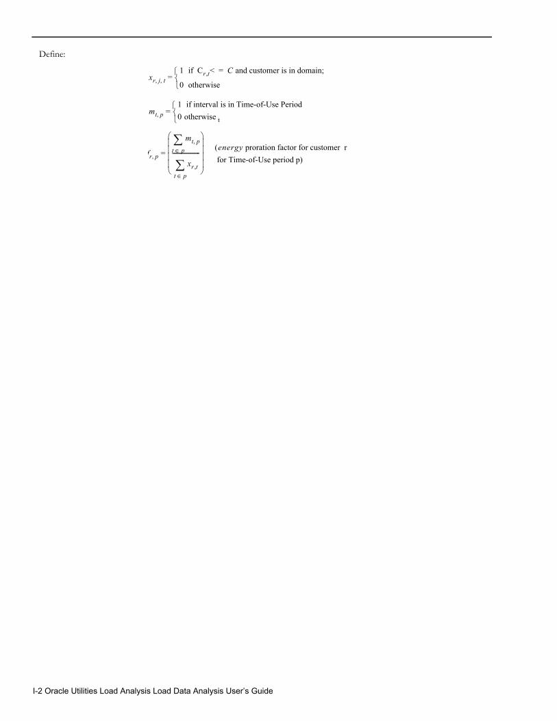
Define:
xr j t, , = 1 if Cr t, < C and customer is in domain; =
0 otherwise
mt p, = 1 if interval is in Time-of-Use Period0 otherwise t
fr p, =
mt p,t p∈
xr t,t p∈
--------------------
(energy proration factor for customer r for Time-of-Use period p)
I-2 Oracle Utilities Load Analysis Load Data Analysis User’s Guide
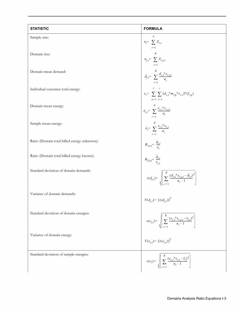
STATISTIC FORMULA
Sample size:
Domain size:
Domain mean demand:
Individual customer total energy:
Domain mean energy:
Sample mean energy:
Ratio (Domain total billed energy unknown):
Ratio (Domain total billed energy known):
Standard deviation of domain demands:
Variance of domain demands:
Standard deviation of domain energies:
Variance of domain energy:
Standard deviation of sample energies:
nt Xr t,r 1=
R
=
nj t, Xr j t,,r 1=
R
=
dj t,dr t, ∗xr j t,,nt
---------------------r 1=
R
=
er dr t, ∗mt p, ∗xr t, ]∗ fr p,( )[
t 1=
T
p 1=
P
=
ej t,er t, ∗xr j t,,nt
---------------------r 1=
R
=
eter t, ∗xr t,nt
------------------r 1=
R
=
R1 t( )dj t,et
-------=
R2 t( )dj t,ej t,-------=
s dj t,( )dr t, ∗xr j t,, dj t,–( )
nt 1–---------------------------------------
2
r 1=
R
=
V dj t,( ) s dj t,( )[ ]2=
s ej t,( )er t, ∗xr j t,, ej t,–( )
nt 1–---------------------------------------
2
r 1=
R
=
V ej t,( ) s ej t,( )[ ]2=
s et( )er t, ∗xr t, et–( )nt 1–
---------------------------------2
r 1=
R
=
Domains Analysis Ratio Equations I-3
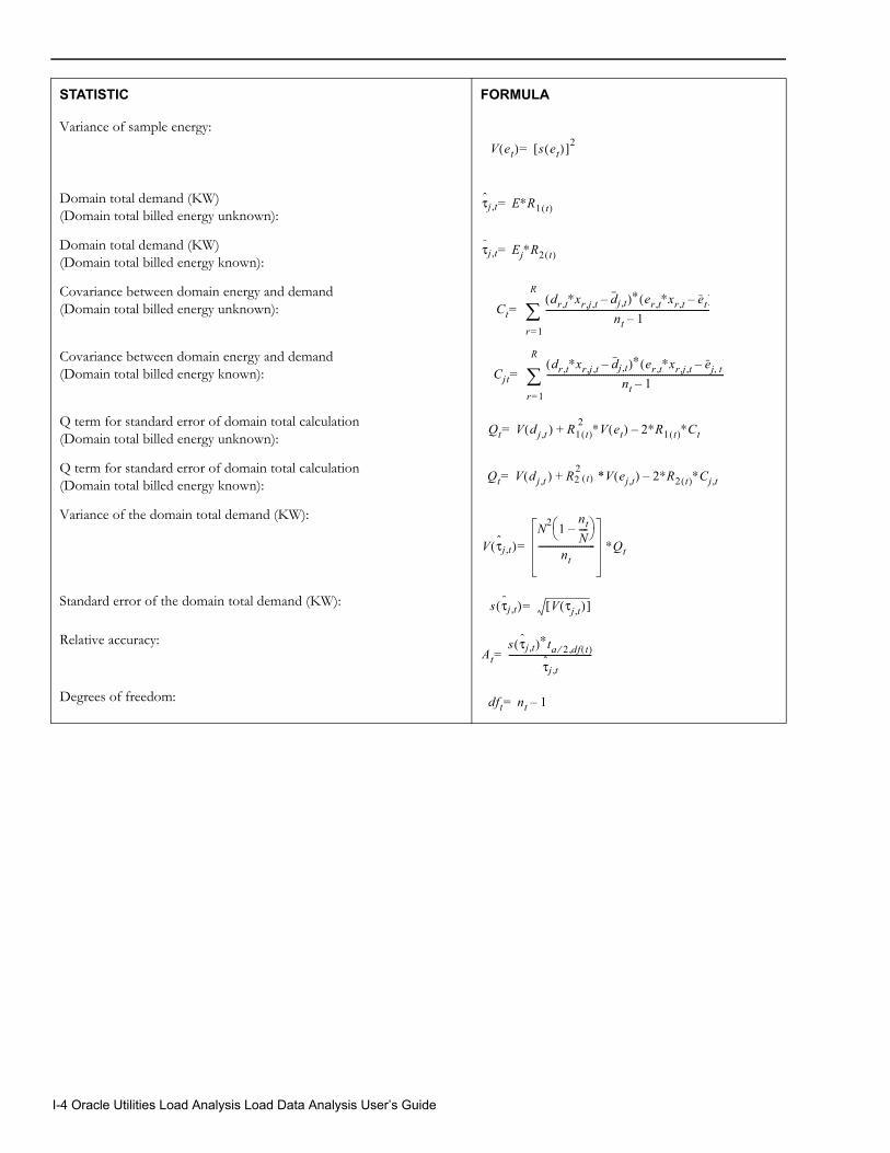
Variance of sample energy:
Domain total demand (KW) (Domain total billed energy unknown):
Domain total demand (KW) (Domain total billed energy known):
Covariance between domain energy and demand(Domain total billed energy unknown):
Covariance between domain energy and demand (Domain total billed energy known):
Q term for standard error of domain total calculation (Domain total billed energy unknown):
Q term for standard error of domain total calculation (Domain total billed energy known):
Variance of the domain total demand (KW):
Standard error of the domain total demand (KW):
Relative accuracy:
Degrees of freedom:
STATISTIC FORMULA
V et( ) s et( )[ ]2=
τj t, E∗R1 t( )=
τj t, Ej∗R2 t( )=
Ctdr t, ∗xr j t,, dj t,–( )∗ er t, ∗xr t, et–( )
nt 1–----------------------------------------------------------------------------
r 1=
R
=
Cjtdr t, ∗xr j t,, dj t,–( )∗ er t, ∗xr j t,, ej t,–( )
nt 1–-----------------------------------------------------------------------------------
r 1=
R
=
Qt V d( j t, ) R1 t( )∗V et( ) 2∗R1 t( )∗Ct–2+=
Qt V d( j t, ) R22 t( ) *V ej t,( ) 2∗R2 t( )∗Cj t,–+=
V τj t,( )N2 1
ntN----–
nt-------------------------- ∗Qt=
s τj t,( ) V τj t,( )[ ]=
Ats τj t,( )∗ta 2 df t( ),⁄
τj t,--------------------------------------=
dft nt 1–=
I-4 Oracle Utilities Load Analysis Load Data Analysis User’s Guide
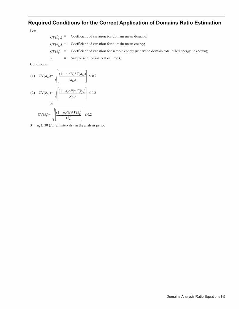
Required Conditions for the Correct Application of Domains Ratio EstimationLet:
= Coefficient of variation for domain mean demand;
= Coefficient of variation for domain mean energy;
= Coefficient of variation for sample energy (use when domain total billed energy unknown);
nt = Sample size for interval of time t;
Conditions:
or
CV dj t,( )
CV ej t,( )
CV et( )
1( ) CV dj t,( ) 1 nt N⁄–( )∗V dj t,( )
dj t,( )--------------------------------------------- 0.2≤=
2( ) CV ej t,( ) 1 nt N⁄–( )∗V ej t,( )ej t,( )
--------------------------------------------- 0.2≤=
CV et( ) 1 nt N⁄–( )∗V et( )et( )
------------------------------------------ 0.2≤=
3) nt 30 for all intervals t in the analysis period( )≥
Domains Analysis Ratio Equations I-5
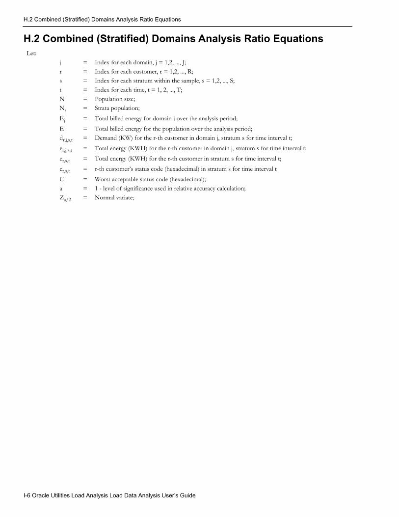
H.2 Combined (Stratified) Domains Analysis Ratio Equations
H.2 Combined (Stratified) Domains Analysis Ratio EquationsLet:
j = Index for each domain, j = 1,2, ..., J;
r = Index for each customer, r = 1,2, ..., R;s = Index for each stratum within the sample, s = 1,2, ..., S;t = Index for each time, t = 1, 2, ..., T;
N = Population size;Ns = Strata population;
Ej = Total billed energy for domain j over the analysis period;
E = Total billed energy for the population over the analysis period;dr,j,s,t = Demand (KW) for the r-th customer in domain j, stratum s for time interval t;
er,j,s,t = Total energy (KWH) for the r-th customer in domain j, stratum s for time interval t;
er,s,t = Total energy (KWH) for the r-th customer in stratum s for time interval t;
cr,s,t = r-th customer’s status code (hexadecimal) in stratum s for time interval t
C = Worst acceptable status code (hexadecimal);a = 1 - level of significance used in relative accuracy calculation;Za/2 = Normal variate;
I-6 Oracle Utilities Load Analysis Load Data Analysis User’s Guide
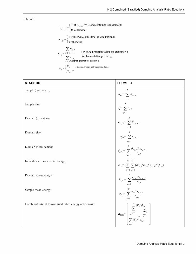
H.2 Combined (Stratified) Domains Analysis Ratio Equations
Define:
xr j s t, , , = 1 if Cr s t,, <= C and customer is in domain;
0 otherwise
mt p, = 1 if interval,tis in Time-of-Use Period p
0 otherwise
fr p, =
mt p,t p∈
xr s t,,t p∈--------------------
(energy proration factor for customer r for Time-of-Use period p)
weighting factor for stratum s
Ws = Ws if externally supplied weighting factor
Ns N⁄
STATISTIC FORMULA
Sample (Strata) size;
Sample size:
Domain (Strata) size:
Domain size:
Domain mean demand:
Individual customer total energy:
Domain mean energy:
Sample mean energy:
Combined ratio (Domain total billed energy unknown):
ns t, Xr s t,,
r 1=
R
=
nt ns t,s 1=
S
=
ns j t,, Xr s j t,,,
r 1=
R
=
nj t, ns j t,,
s 1=
S
=
dj s t,,dr j s t,,, ∗xr j s t,,,
ns t,-------------------------------
r 1=
R
=
er s, dr s t,, ∗mt p, ∗xr s t,, ]∗ fr p,( )[t 1=
T
p 1=
P
=
es j, t,er s j,, ∗xr s j t,,,
ns t,---------------------------
r 1=
R
=
es t,er s, ∗xr s t,,ns t,
-----------------------r 1=
R
=
R1 t( )
Ws∗ds j t,,
dj t,s 1=
S
Ws∗ es t, et=
s 1=
S
-------------------------------------------=
Domains Analysis Ratio Equations I-7
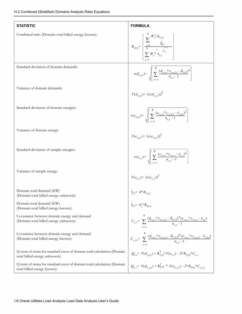
H.2 Combined (Stratified) Domains Analysis Ratio Equations
Combined ratio (Domain total billed energy known):
Standard deviation of domain demands:
Variance of domain demands:
Standard deviation of domain energies:
Variance of domain energy:
Standard deviation of sample energies:
Variance of sample energy:
Domain total demand (KW)(Domain total billed energy unknown):
Domain total demand (KW)(Domain total billed energy known):
Covariance between domain energy and demand(Domain total billed energy unknown):
Covariance between domain energy and demand (Domain total billed energy known):
Q term of strata for standard error of domain total calculation (Domain total billed energy unknown):
Q term of strata for standard error of domain total calculation (Domain total billed energy known):
STATISTIC FORMULA
R2 t( )
Ws∗ds j t,,
dj t,s 1=
S
Ws∗ es t, ej t,=
s 1=
S
-----------------------------------------------=
s ds j, t,( )dr s t,, ∗xr s j, t,, ds j, t,–( )
ns t, 1–-------------------------------------------------
2
r 1=
R
=
V ds j, t,( ) s ds j t,,( )[ ]2=
s es j, t,( )er s t,, ∗xr s j, t,, es j, t,–( )
ns t, 1–-------------------------------------------------
2
r 1=
R
=
V es j, t,( ) s es j, t,( )[ ]2=
s es t,( )er s t,, ∗xr s t,, es t,–( )
ns t, 1–---------------------------------------------
2
r 1=
R
=
V es t,( ) s es t,( )[ ]2=
τj t, E∗R1 t( )=
τj t, Ej∗R2 t( )=
Cs t,dr s t,, ∗xr s j t,,, ds j t,,–( )∗ er s t,, ∗xr s t,, es t,–( )
ns t, 1–----------------------------------------------------------------------------------------------------
r 1=
R
=
Cs j t,,dr s t,, ∗xr s j t,,, ds j t,,–( )∗ er s t,, ∗xr s j t,,, es j t,,–( )
ns t, 1–----------------------------------------------------------------------------------------------------------
r 1=
R
=
Qs t, V d( s j, t, ) R1 t( )∗V es t,( ) 2∗R1 t( )∗Cs t,–2+=
Qs t, V d( s j t,, ) R22 t( ) * V es j t,,( ) 2∗R2 t( )∗Cs j t,,–+=
I-8 Oracle Utilities Load Analysis Load Data Analysis User’s Guide
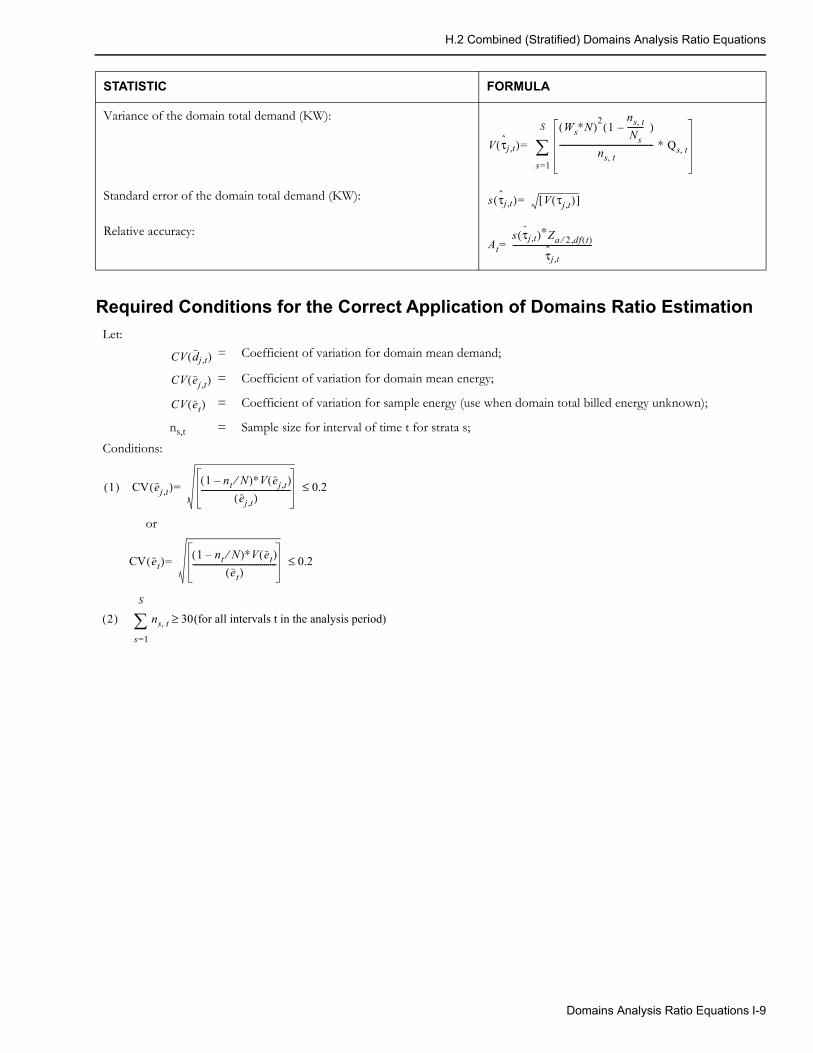
H.2 Combined (Stratified) Domains Analysis Ratio Equations
Required Conditions for the Correct Application of Domains Ratio Estimation
Variance of the domain total demand (KW):
Standard error of the domain total demand (KW):
Relative accuracy:
STATISTIC FORMULA
V τj t,( )Ws∗N( )2 1(
ns t,Ns-------- )–
ns t,----------------------------------------------- ∗ Qs t,
s 1=
S
=
s τj t,( ) V τj t,( )[ ]=
Ats τj t,( )∗Za 2 df t( ),⁄
τj t,----------------------------------------=
Let:= Coefficient of variation for domain mean demand;
= Coefficient of variation for domain mean energy;
= Coefficient of variation for sample energy (use when domain total billed energy unknown);
ns,t = Sample size for interval of time t for strata s;
Conditions:
or
CV dj t,( )
CV ej t,( )
CV et( )
1( ) CV ej t,( ) 1 nt N⁄–( )∗V ej t,( )ej t,( )
--------------------------------------------- 0.2≤=
CV et( ) 1 nt N⁄–( )∗V et( )et( )
------------------------------------------ 0.2≤=
2( ) ns t, 30(for all intervals t in the analysis period)≥s 1=
S
Domains Analysis Ratio Equations I-9

H.3 Average Day Statistics
H.3 Average Day StatisticsAverage day statistics are computed from a sample across a set of customers and across a set of days. Since samples from the same customer or separate days are not completely independent, Oracle Utilities Load Analysis cannot rigorously compute standard error, degrees of freedom or relative accuracy statistics. Instead Oracle Utilities Load Analysis reports a Relative Error Measure using the standard error equation, where the sample size is the total number of observations across customers and days. This Relative Error cannot be interpreted as a standard error because it would overstate the accuracy of the estimates.
I-10 Oracle Utilities Load Analysis Load Data Analysis User’s Guide
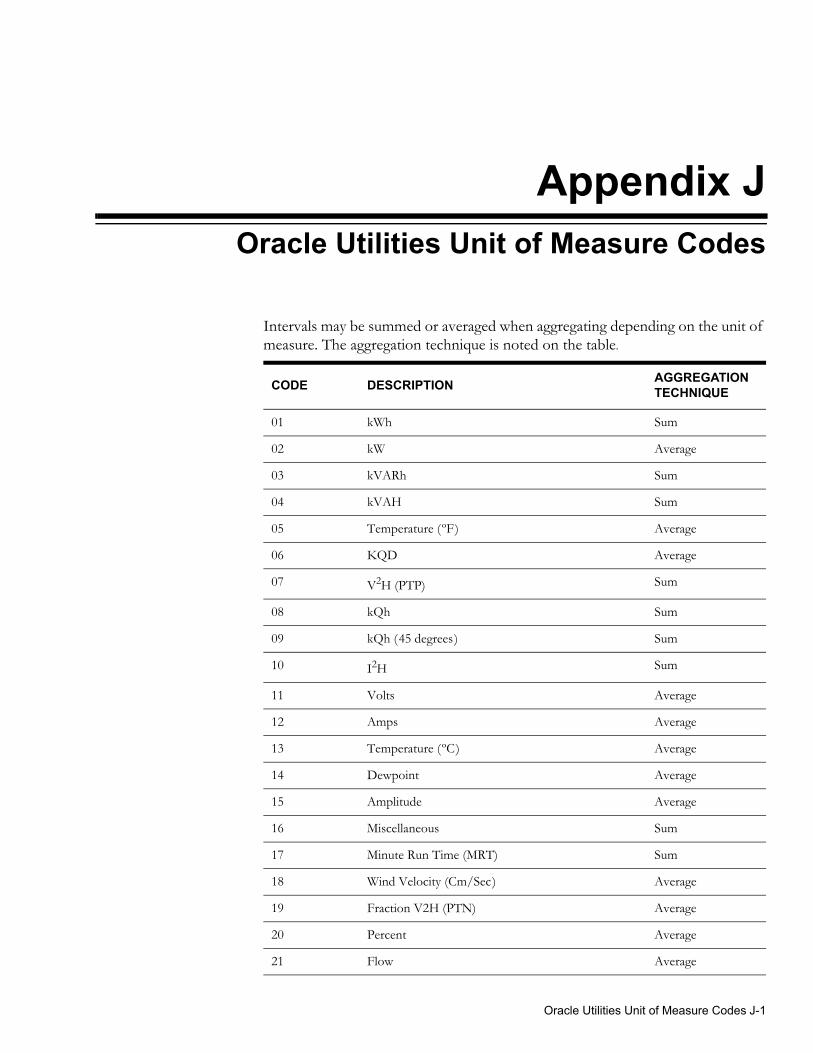
Appendix JOracle Utilities Unit of Measure Codes
Intervals may be summed or averaged when aggregating depending on the unit of measure. The aggregation technique is noted on the table.
CODE DESCRIPTION AGGREGATION TECHNIQUE
01 kWh Sum
02 kW Average
03 kVARh Sum
04 kVAH Sum
05 Temperature (ºF) Average
06 KQD Average
07 V2H (PTP) Sum
08 kQh Sum
09 kQh (45 degrees) Sum
10 I2H Sum
11 Volts Average
12 Amps Average
13 Temperature (ºC) Average
14 Dewpoint Average
15 Amplitude Average
16 Miscellaneous Sum
17 Minute Run Time (MRT) Sum
18 Wind Velocity (Cm/Sec) Average
19 Fraction V2H (PTN) Average
20 Percent Average
21 Flow Average
Oracle Utilities Unit of Measure Codes J-1
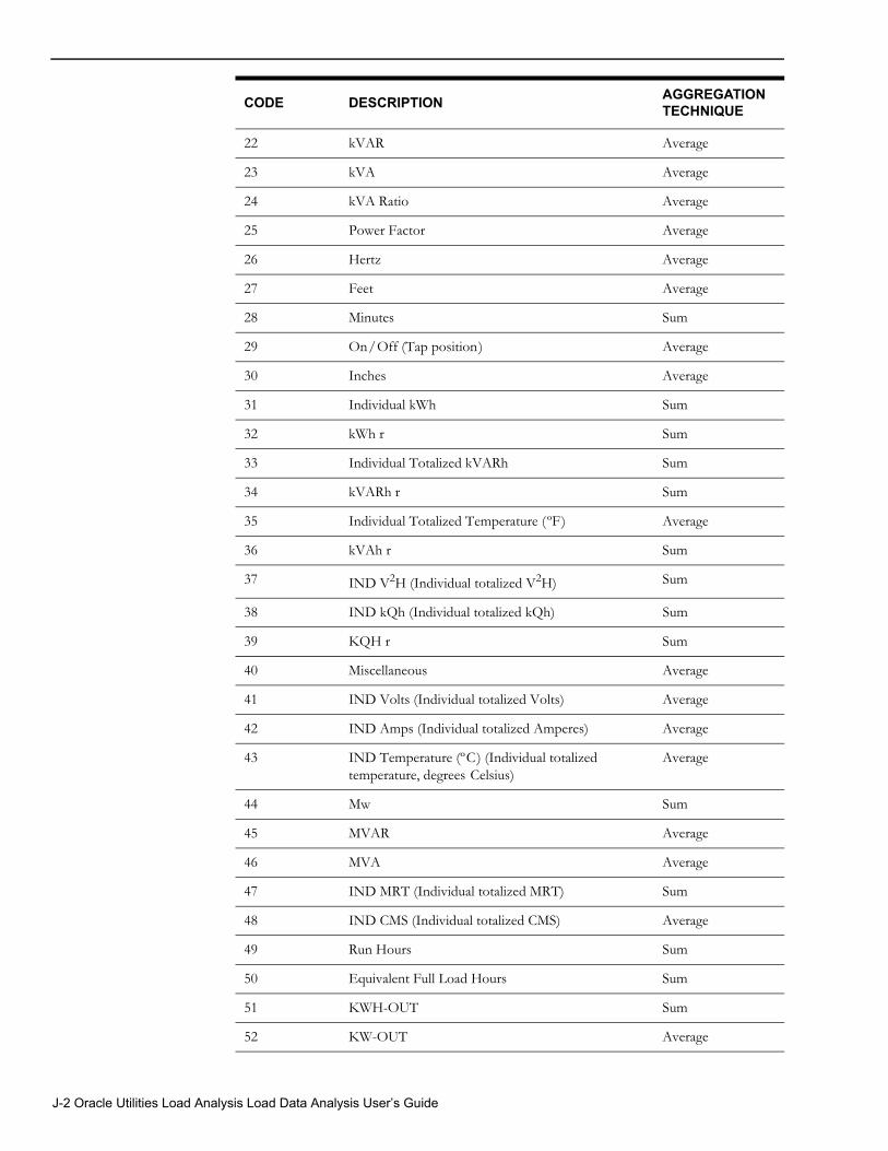
22 kVAR Average
23 kVA Average
24 kVA Ratio Average
25 Power Factor Average
26 Hertz Average
27 Feet Average
28 Minutes Sum
29 On/Off (Tap position) Average
30 Inches Average
31 Individual kWh Sum
32 kWh r Sum
33 Individual Totalized kVARh Sum
34 kVARh r Sum
35 Individual Totalized Temperature (ºF) Average
36 kVAh r Sum
37 IND V2H (Individual totalized V2H) Sum
38 IND kQh (Individual totalized kQh) Sum
39 KQH r Sum
40 Miscellaneous Average
41 IND Volts (Individual totalized Volts) Average
42 IND Amps (Individual totalized Amperes) Average
43 IND Temperature (ºC) (Individual totalized temperature, degrees Celsius)
Average
44 Mw Sum
45 MVAR Average
46 MVA Average
47 IND MRT (Individual totalized MRT) Sum
48 IND CMS (Individual totalized CMS) Average
49 Run Hours Sum
50 Equivalent Full Load Hours Sum
51 KWH-OUT Sum
52 KW-OUT Average
CODE DESCRIPTION AGGREGATION TECHNIQUE
J-2 Oracle Utilities Load Analysis Load Data Analysis User’s Guide
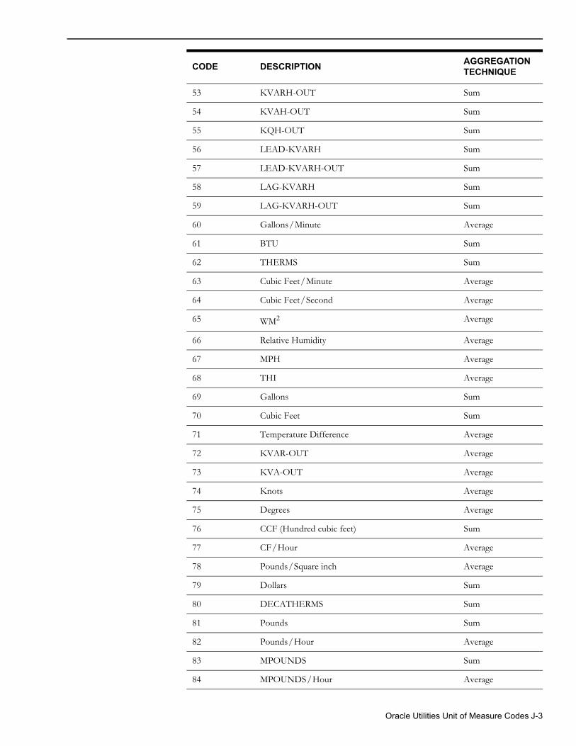
53 KVARH-OUT Sum
54 KVAH-OUT Sum
55 KQH-OUT Sum
56 LEAD-KVARH Sum
57 LEAD-KVARH-OUT Sum
58 LAG-KVARH Sum
59 LAG-KVARH-OUT Sum
60 Gallons/Minute Average
61 BTU Sum
62 THERMS Sum
63 Cubic Feet/Minute Average
64 Cubic Feet/Second Average
65 WM2 Average
66 Relative Humidity Average
67 MPH Average
68 THI Average
69 Gallons Sum
70 Cubic Feet Sum
71 Temperature Difference Average
72 KVAR-OUT Average
73 KVA-OUT Average
74 Knots Average
75 Degrees Average
76 CCF (Hundred cubic feet) Sum
77 CF/Hour Average
78 Pounds/Square inch Average
79 Dollars Sum
80 DECATHERMS Sum
81 Pounds Sum
82 Pounds/Hour Average
83 MPOUNDS Sum
84 MPOUNDS/Hour Average
CODE DESCRIPTION AGGREGATION TECHNIQUE
Oracle Utilities Unit of Measure Codes J-3
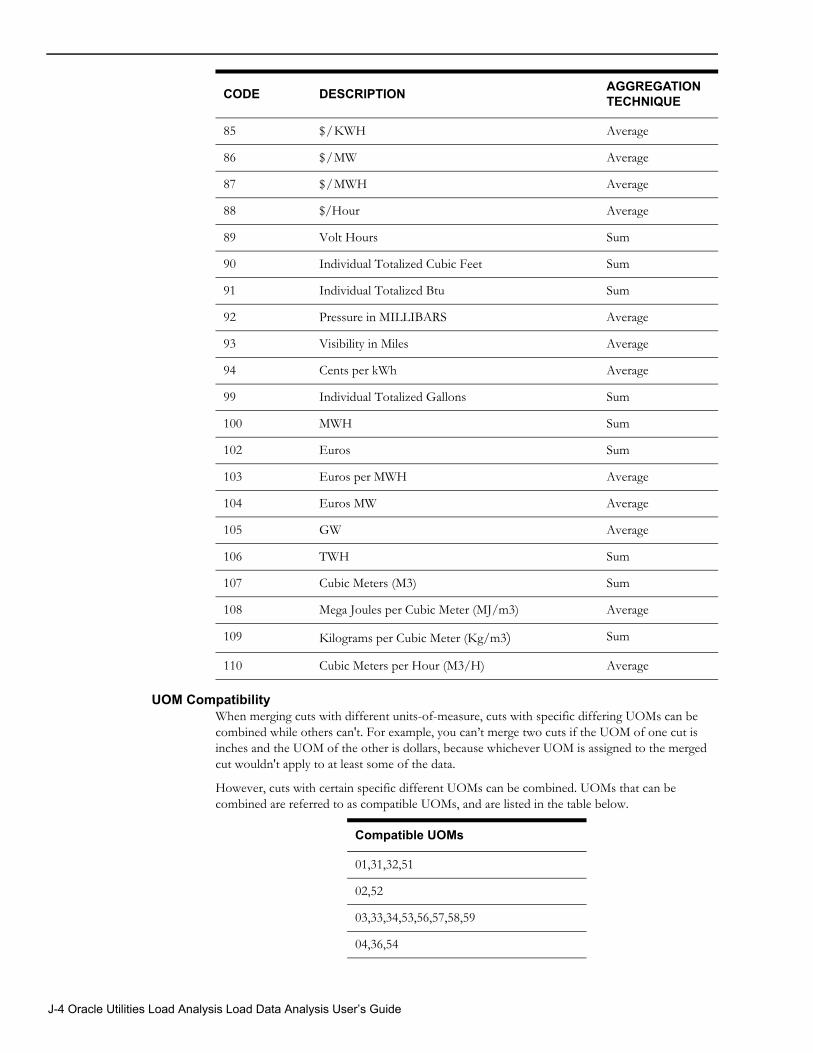
UOM CompatibilityWhen merging cuts with different units-of-measure, cuts with specific differing UOMs can be combined while others can't. For example, you can’t merge two cuts if the UOM of one cut is inches and the UOM of the other is dollars, because whichever UOM is assigned to the merged cut wouldn't apply to at least some of the data.
However, cuts with certain specific different UOMs can be combined. UOMs that can be combined are referred to as compatible UOMs, and are listed in the table below.
85 $/KWH Average
86 $/MW Average
87 $/MWH Average
88 $/Hour Average
89 Volt Hours Sum
90 Individual Totalized Cubic Feet Sum
91 Individual Totalized Btu Sum
92 Pressure in MILLIBARS Average
93 Visibility in Miles Average
94 Cents per kWh Average
99 Individual Totalized Gallons Sum
100 MWH Sum
102 Euros Sum
103 Euros per MWH Average
104 Euros MW Average
105 GW Average
106 TWH Sum
107 Cubic Meters (M3) Sum
108 Mega Joules per Cubic Meter (MJ/m3) Average
109 Kilograms per Cubic Meter (Kg/m3) Sum
110 Cubic Meters per Hour (M3/H) Average
CODE DESCRIPTION AGGREGATION TECHNIQUE
Compatible UOMs
01,31,32,51
02,52
03,33,34,53,56,57,58,59
04,36,54
J-4 Oracle Utilities Load Analysis Load Data Analysis User’s Guide
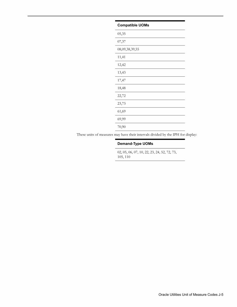
These units of measures may have their intervals divided by the IPH for display:
05,35
07,37
08,09,38,39,55
11,41
12,42
13,43
17,47
18,48
22,72
23,73
61,69
69,99
70,90
Demand-Type UOMs
02, 05, 06, 07, 10, 22, 23, 24, 52, 72, 73, 105, 110
Compatible UOMs
Oracle Utilities Unit of Measure Codes J-5

J-6 Oracle Utilities Load Analysis Load Data Analysis User’s Guide
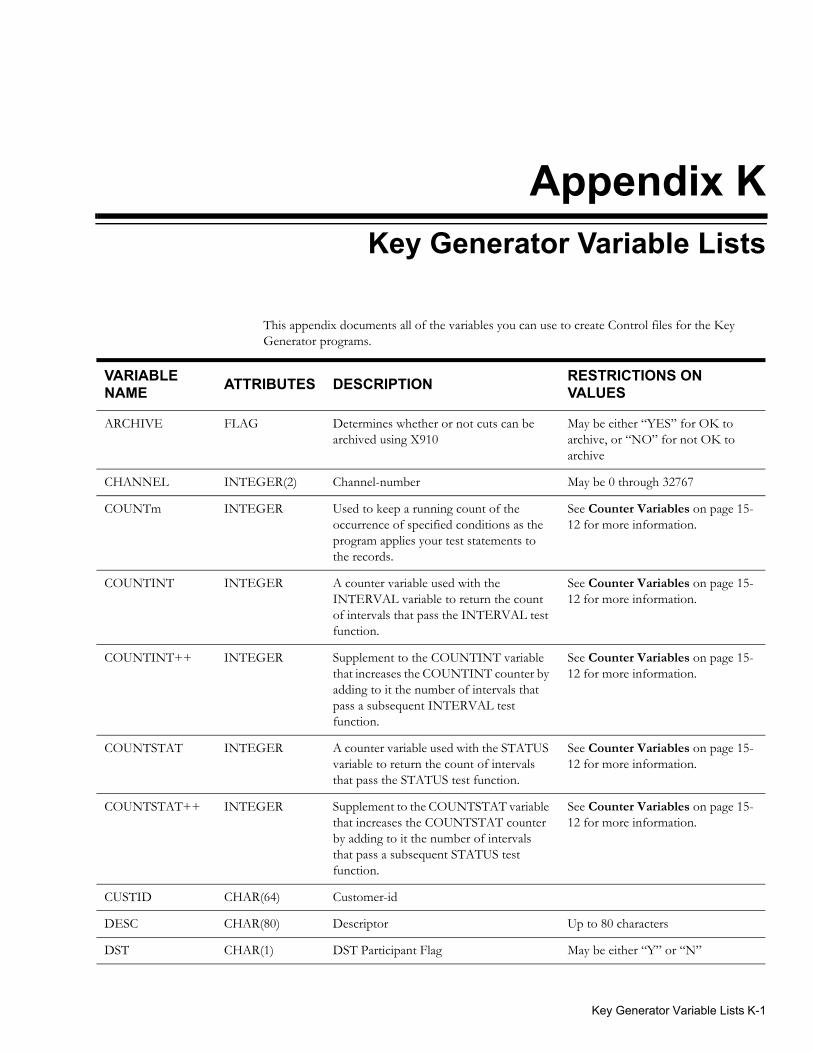
Appendix KKey Generator Variable Lists
This appendix documents all of the variables you can use to create Control files for the Key Generator programs.
VARIABLENAME ATTRIBUTES DESCRIPTION RESTRICTIONS ON
VALUES
ARCHIVE FLAG Determines whether or not cuts can be archived using X910
May be either “YES” for OK to archive, or “NO” for not OK to archive
CHANNEL INTEGER(2) Channel-number May be 0 through 32767
COUNTm INTEGER Used to keep a running count of the occurrence of specified conditions as the program applies your test statements to the records.
See Counter Variables on page 15-12 for more information.
COUNTINT INTEGER A counter variable used with the INTERVAL variable to return the count of intervals that pass the INTERVAL test function.
See Counter Variables on page 15-12 for more information.
COUNTINT++ INTEGER Supplement to the COUNTINT variable that increases the COUNTINT counter by adding to it the number of intervals that pass a subsequent INTERVAL test function.
See Counter Variables on page 15-12 for more information.
COUNTSTAT INTEGER A counter variable used with the STATUS variable to return the count of intervals that pass the STATUS test function.
See Counter Variables on page 15-12 for more information.
COUNTSTAT++ INTEGER Supplement to the COUNTSTAT variable that increases the COUNTSTAT counter by adding to it the number of intervals that pass a subsequent STATUS test function.
See Counter Variables on page 15-12 for more information.
CUSTID CHAR(64) Customer-id
DESC CHAR(80) Descriptor Up to 80 characters
DST CHAR(1) DST Participant Flag May be either “Y” or “N”
Key Generator Variable Lists K-1
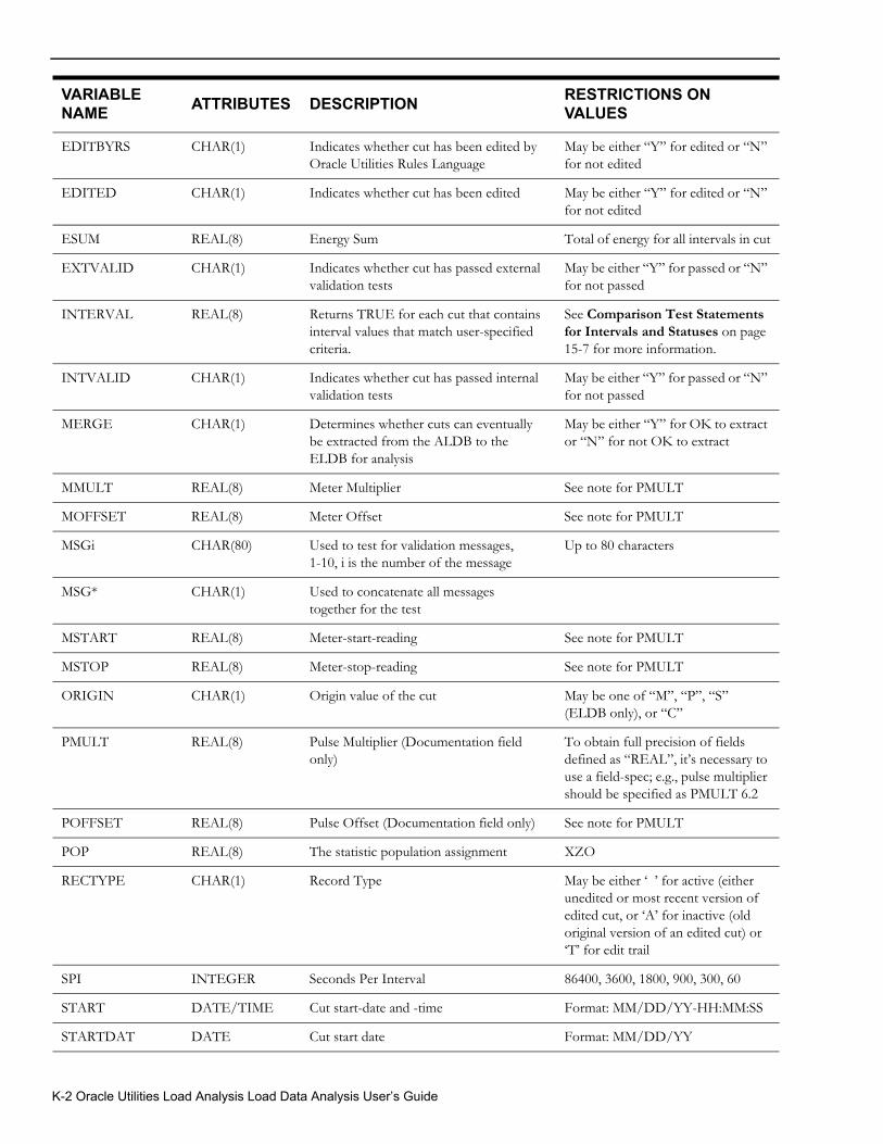
EDITBYRS CHAR(1) Indicates whether cut has been edited by Oracle Utilities Rules Language
May be either “Y” for edited or “N” for not edited
EDITED CHAR(1) Indicates whether cut has been edited May be either “Y” for edited or “N” for not edited
ESUM REAL(8) Energy Sum Total of energy for all intervals in cut
EXTVALID CHAR(1) Indicates whether cut has passed external validation tests
May be either “Y” for passed or “N” for not passed
INTERVAL REAL(8) Returns TRUE for each cut that contains interval values that match user-specified criteria.
See Comparison Test Statements for Intervals and Statuses on page 15-7 for more information.
INTVALID CHAR(1) Indicates whether cut has passed internal validation tests
May be either “Y” for passed or “N” for not passed
MERGE CHAR(1) Determines whether cuts can eventually be extracted from the ALDB to the ELDB for analysis
May be either “Y” for OK to extract or “N” for not OK to extract
MMULT REAL(8) Meter Multiplier See note for PMULT
MOFFSET REAL(8) Meter Offset See note for PMULT
MSGi CHAR(80) Used to test for validation messages,1-10, i is the number of the message
Up to 80 characters
MSG* CHAR(1) Used to concatenate all messagestogether for the test
MSTART REAL(8) Meter-start-reading See note for PMULT
MSTOP REAL(8) Meter-stop-reading See note for PMULT
ORIGIN CHAR(1) Origin value of the cut May be one of “M”, “P”, “S” (ELDB only), or “C”
PMULT REAL(8) Pulse Multiplier (Documentation field only)
To obtain full precision of fields defined as “REAL”, it’s necessary to use a field-spec; e.g., pulse multiplier should be specified as PMULT 6.2
POFFSET REAL(8) Pulse Offset (Documentation field only) See note for PMULT
POP REAL(8) The statistic population assignment XZO
RECTYPE CHAR(1) Record Type May be either ‘ ’ for active (either unedited or most recent version of edited cut, or ‘A’ for inactive (old original version of an edited cut) or ‘T’ for edit trail
SPI INTEGER Seconds Per Interval 86400, 3600, 1800, 900, 300, 60
START DATE/TIME Cut start-date and -time Format: MM/DD/YY-HH:MM:SS
STARTDAT DATE Cut start date Format: MM/DD/YY
VARIABLENAME ATTRIBUTES DESCRIPTION RESTRICTIONS ON
VALUES
K-2 Oracle Utilities Load Analysis Load Data Analysis User’s Guide
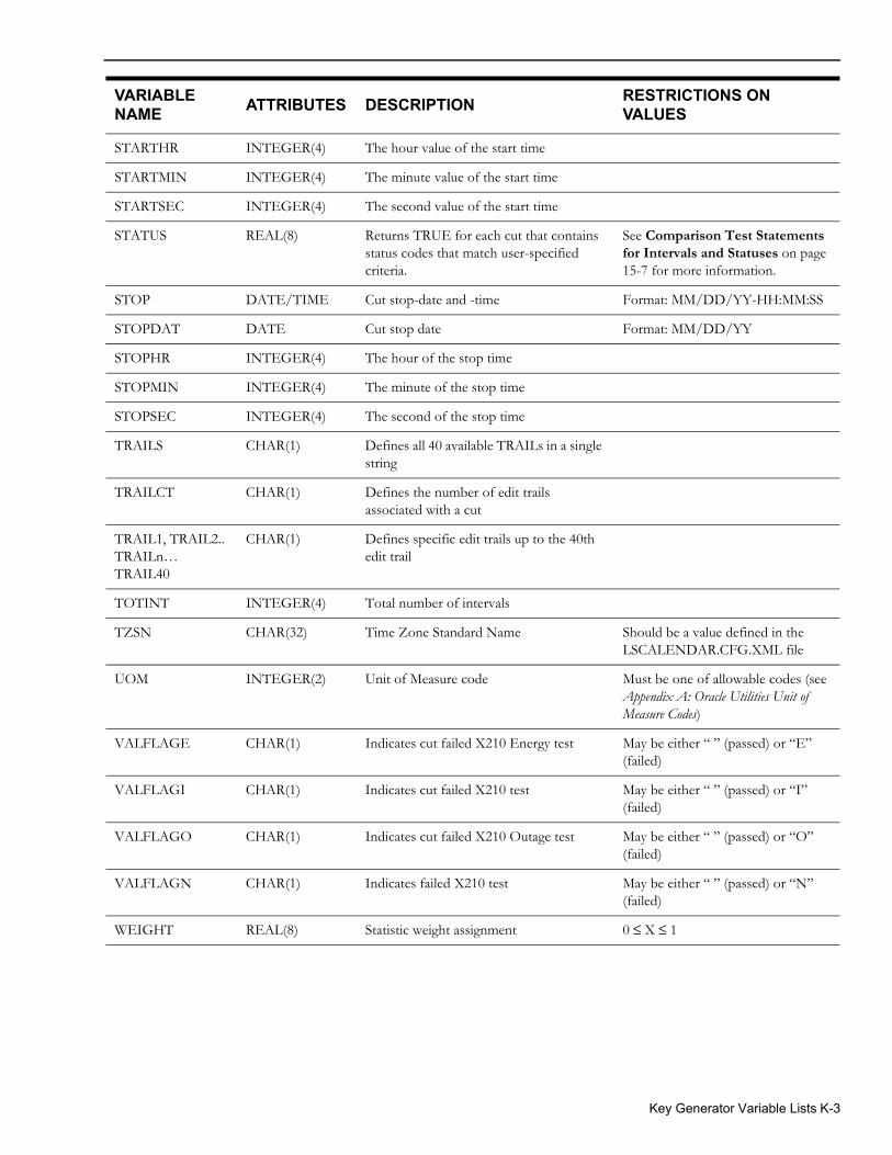
STARTHR INTEGER(4) The hour value of the start time
STARTMIN INTEGER(4) The minute value of the start time
STARTSEC INTEGER(4) The second value of the start time
STATUS REAL(8) Returns TRUE for each cut that contains status codes that match user-specified criteria.
See Comparison Test Statements for Intervals and Statuses on page 15-7 for more information.
STOP DATE/TIME Cut stop-date and -time Format: MM/DD/YY-HH:MM:SS
STOPDAT DATE Cut stop date Format: MM/DD/YY
STOPHR INTEGER(4) The hour of the stop time
STOPMIN INTEGER(4) The minute of the stop time
STOPSEC INTEGER(4) The second of the stop time
TRAILS CHAR(1) Defines all 40 available TRAILs in a single string
TRAILCT CHAR(1) Defines the number of edit trails associated with a cut
TRAIL1, TRAIL2.. TRAILn… TRAIL40
CHAR(1) Defines specific edit trails up to the 40th edit trail
TOTINT INTEGER(4) Total number of intervals
TZSN CHAR(32) Time Zone Standard Name Should be a value defined in the LSCALENDAR.CFG.XML file
UOM INTEGER(2) Unit of Measure code Must be one of allowable codes (see Appendix A: Oracle Utilities Unit of Measure Codes)
VALFLAGE CHAR(1) Indicates cut failed X210 Energy test May be either “ ” (passed) or “E” (failed)
VALFLAGI CHAR(1) Indicates cut failed X210 test May be either “ ” (passed) or “I” (failed)
VALFLAGO CHAR(1) Indicates cut failed X210 Outage test May be either “ ” (passed) or “O” (failed)
VALFLAGN CHAR(1) Indicates failed X210 test May be either “ ” (passed) or “N” (failed)
WEIGHT REAL(8) Statistic weight assignment 0 ≤ X ≤ 1
VARIABLENAME ATTRIBUTES DESCRIPTION RESTRICTIONS ON
VALUES
Key Generator Variable Lists K-3

K-4 Oracle Utilities Load Analysis Load Data Analysis User’s Guide
Index
AAbbreviations 20-14, 20-29, 20-30Adding data 15-2Aggregate Load Analysis 9-1Control file 9-3Environment file 9-6Statistics computed by (list of) 2-8
Aggregation 20-11ALDB, see Archive Load Database 2-10ALDB/CLDB Extraction, see Load Data Extraction 5-2Analysis Control File (TGY37A.CTL) 20-8Analysis Environment File (TGY37B.ENV) 20-10Analyzing non-contiguous periods 20-11Archive flag 3-8, 5-5Archive Load Database (ALDB) 2-10
Extracting data from 5-3Archive/Delete 17-3–??
Control file 17-4Output reports 17-4
Arithmetic operations (Transformation) 15-2, 15-3, 15-5
Average day demandsHow Load Analysis computes 2-3Reports 12-2
Average Day Profiles 20-3Average Day Statistics Output File Format 20-27Average Day Type Reports 20-6Average Day Type Statistics
abbreviations 20-29Average Day Type Statistics Report 20-6, 20-18Average Day-Type Statistics Report Command 20-13Average-Day Type statistics 20-18AVG commands 20-13AVGREPORT Command 20-30
BBilled Energy 7-3Billed Energy Program 13-1–??
Control File 13-3Environment File 13-8
Billing Cycle parameter 20-8Breakpoint Command 10-10breakpoints 10-3, 10-5, 10-8, 10-12
CCAF, see Customer Attribute File 2-9CHAnge command (Load Data Editor) 6-4Channel-number 3-4Class function (Transformation) 15-7Classification of Interval Data 20-31CLDB, see Current Load Database 2-10Coincident Peak Analysis Program 2-3Combining multiple channels 20-8Control File Record Format 20-29Control files
Aggregate Load Analysis 9-3Billed Energy 13-3Direct Output 16-5Domains Analysis Mean Per Unit
Domains Analysis Ratio 11-4General description 4-2Key Generators 14-20Load Data Editor 6-3, 6-4Load Data Extraction 5-8Load Data Reporter 12-13Ratio Analysis 7-7, 8-4SLDB Retrieval 17-5Standard Load Analysis 7-7, 8-4Statistical Package Interface 16-17, 16-23Summary Reporters 12-16, 18-2Time Series Reporter 12-4, 12-5, 12-6Transformation 15-2, 15-17
ConventionsFormat, Used in the Guide i-ii, 11-1ICA 20-29Used in Load Analysis 4-3
COPy command (Load Data Editor) 6-4Cost of Service Interface 1-7Cost of service studies 1-2Counting records
How to 14-4Current Load Database (CLDB) 2-10
Extracting data from 5-3Curtailment Periods 20-22Customer Analysis Program (ICA)
Overview 20-29Customer Attribute File (CAF) 2-9Customer statistics 2-4Customer-id 3-4Cut 3-2, 3-3
Index-1
Differences between ELDB cuts and CLDB cuts 3-4Simulated (statistics record) 3-8
Cut key 3-3Cut series 3-3Cut series key 3-3
DD240 - ALDB/CLDB Extraction
Input filesEnvironment File
Aggregate command 5-7Date command 5-6Source command 5-7
Data dumps 12-7Databases 2-9–2-12
Maintenance 17-2Date Record 20-16Daytype Analysis (E760) 19-1Deleting data
From the ELDB 17-3Demand dumps 12-7Demand Period File 20-8
application 20-5setup 20-16
Demand Period File Record Format 20-29demand periods 20-4Demand side management 1-2Descriptor
On ELDB load data records 3-5On statistics records 3-10
Direct Input 5-2Direct Output 16-13–??Direct Output Formats
Descriptions of Binary Daily Energy Format 16-15Descriptions of Character Daily Energy Format 16-15Descriptions of Daily Energy Format 16-15Descriptions of Standard Format 16-13
Direct Output ProgramControl File 16-5Environment File 16-6
Dividing data 15-2Domains Analysis 2-3Domains Analysis Mean Per Unit Program 11-2
Control File 11-4Environment file 11-7Output 11-22
Domains Analysis Ratio Program 11-1Control File 11-4Environment file 11-7Output 11-22
Duration function (Transformation) 15-7
EE220 - Manual Entry (ELDB) 5-2E230 - Billed Energy 13-1
InputsControl File 13-3Cycle File 13-7Environment File 13-8
Aggregate command 13-9
Date command 13-8Length command 13-9Prorate command 13-9Quality command 13-9Replace command 13-9Type command 13-8
ProcessingProcessing, description of 13-10
E240 - ALDB/CLDB Extraction 5-1Input files
Control File 5-8Environment File 5-6
ProcessingProcessing, description of 5-8, 5-9
E350 - Domains Analysis Mean Per Unit (Optional Extension)Inputs
Control File 11-4, 11-7ELDB cuts 11-4, 11-7Environment File 11-7, 11-12
Aggregate command 11-9Alpha command 11-17Assign command 11-11Date command 11-9Domain command 11-12Drop command 11-10Group command 11-15ICS command 11-15Key command 11-15Minimum command 11-17Peak command 11-14Population command 11-13Prorate command 11-10Quality command 11-10Report command 11-15Rolling command 11-10Season command 11-14Strata command 11-11Write command 11-16
Holiday File 11-17Season File 11-17Time-of-Use File 11-17User-Specified Day File 11-17
Output filesIndividual Customer Statistics File 11-23Statistics Written to the ELDB 11-22
Output reportsStatistics Written to the ELDB Report 11-23
ProcessingProcessing, description of 11-17, 11-19
E360 - Domains Analysis Ratio (Optional Extension)Inputs
Control File 11-4, 11-7ELDB cuts 11-4, 11-7Environment File 11-7, 11-12
Aggregate command 11-9
Index-2
Alpha command 11-17Assign command 11-11Billing command 11-11Date command 11-9Domain command 11-12Drop command 11-10Energy command 11-13Group command 11-15Minimum command 11-17Peak command 11-14Population command 11-13Prorate command 11-10Quality command 11-10Report command 11-15Rolling command 11-10Schedule command 11-14Season command 11-14Strata command 11-11Write command 11-16
Holiday File 11-17Season File 11-17Time-of-Use File 11-17User-Specified Day File 11-17
Output filesIndividual Customer Statistics File 11-23Statistics Written to the ELDB 11-22
ProcessingProcessing, description of 11-19, 11-22
E710 - Statistical Package InterfaceInputs
Control File 16-17, 16-23Data 16-17Environment File 16-18
Aggregate command 16-18Date command 16-18, 16-25Quality command 16-19Source command 16-19
Output filesFormatted Data Matrix 16-20Header Variable File 16-20
Output reportsEnvironment Report 16-20Execution Log 16-20Summary Report 16-20
ProcessingProcessing, description of 16-19
E720 - Direct Output 16-15Inputs
Control File 16-5Data 16-5Environment File
24HRADJ command 16-7Aggregate command 16-7Daily command 16-8Daily Energy Command 16-15
Daily Energy command 16-15Date command 16-9Quality command 16-10Source command 16-10Status command 16-10
Output filesSequential Dataset
Binary Daily Energy Format 16-15Character Daily Energy Format 16-15Standard Format 16-13
ProcessingProcessing, description of 16-12
Edit commandsCorrection commands 6-3Cut commands 6-3Summary of 6-4
Edit flag 3-8, 5-5Edit trails
On ELDB load data records 3-5On statistics records 3-10
Editor, see Load Data Editor 6-2ELDB Load Data Editor, see Load Data Editor 6-3ELDB Summary Reporter, see Summary Reporters 12-2ELDB, see Extracted Load Database 2-9END Statement 20-17Energy
On ELDB load data records 3-5On statistics records 3-10
Energy dumps 12-7Entire period demands
How Load Analysis computes 2-3Reports 12-2
Environment FileSchedule Command 20-9Season Command 20-9
Environment File Record Format 20-29Environment File Write Command 20-18Environment files
Aggregate Load Analysis 9-6Billed Energy 13-8Direct Output 16-5Domains Analysis Mean Per Unit
Domains Analysis Ratio 11-7General description 4-2Load Data Extraction 5-6Load Data Reporter 12-8, 12-10, 12-13Ratio Analysis 7-8, 7-10, 7-11, 7-15, 7-16, 8-5, 8-6,
8-8Standard Load Analysis 7-8, 7-10, 7-11, 7-15, 7-16, 8-
5, 8-6, 8-8Statistical Package Interface 16-18Summary Reporters 12-16, 18-3Time Series Reporter 12-3Transformation 15-15, 15-17
Environment reportsGeneral definition 4-2
ERAse command (Load Data Editor) 6-4Execution logs
General definition 4-2Exponentiating data (Transformation) 15-3
Index-3
Externally valid flag 3-8, 5-4Extracted Load Database (ELDB) 2-9
Reporting the contents of 12-15Extracting data
From the ALDB and/or CLDB 5-2
FFalse clauses 14-7Flags 5-4
Archive 3-8, 5-5Edited 3-8, 5-5Externally Valid 3-8, 5-4Internally Valid 3-8, 5-4Merge 3-8, 5-5
FormulasEstimate of Hourly Class Total Demand 7-2
GGroup Command 20-13
HHeader
On ELDB load data records 3-4On statistics records 3-10
Help, how to get i-iiiHoliday file
Modifying 7-23Holiday File Record Format 20-29
IICA
on the CLDB 20-6on the ELDB 20-6
ICA capabilities 20-2ICA Overview 20-3illegal commands 12-7Individual Customer Analysis Environment File
format 20-10Individual Customer Analysis Environment Report 20-18Individual Customer Definition Report 20-18Individual Customer Statistics 20-2Individual customer statistics 2-4, 7-15, 7-28, 8-8, 11-15,
11-23Individual Customer Statistics File 20-18Input files
General description (refer to program name for specific files) 4-2
Inputting dataOverview 2-10To the ELDB 5-2
Internally valid flag 3-8, 5-4Interval data 2-3, 3-4
Modifying 6-7, 15-2On ELDB load data records 3-6On statistics records 3-10Reporting 12-2, 12-7
KKEY command (Load Data Editor) 6-5
Key Generators 14-2Control file 14-20Control language 14-3
Counting records, How to 14-4Output key file 14-22Output reports 14-22
KeysCut 3-3Cut series 3-3
Llabels
sample 14-6Late Cut Reporter 1-7Load Analysis Subsystem
Databases 2-9Overview 2-2, 2-3Programs 2-9
Load data 1-2Collection 1-4Recorders 1-2Records 3-2
Load Data Editor 6-2Control file 6-3, 6-4Differences between ELDB and CLDB 6-3Output reports 6-7
Load Data Extraction 5-2Control file 5-8Environment file 5-6
Load Data Management Subsystem 1-5Load Data Reporter 12-2, 12-7–??
Control files 12-13Environment file 12-8, 12-10, 12-12Output reports 6-3
Load profiles 1-2Load research 1-2, 1-3, 1-4
MManual Entry 5-2Mask function (Transformation) 15-9Masking data (Transformation) 15-9Mean per unit analysis 7-2Merge flag 3-8, 5-5Meter data 3-5Minutes-per-Interval
On statistics records 3-10Modifying data
Overview 2-10Using the Transformation Program 15-2–??
Modifying required input files 20-6Modifying the Billing Cycle File (TGY23E.CYC) 20-15Modifying the Demand Period File (TGY37E.DEM) 20-16Modifying the Season File (TGY31E.SEA) 20-15Modifying the Time-of-Use Schedule File (TGY31D.TOU) 20-15MONthly keyword 20-11Monthly Summary Report 20-11, 20-18Multiplying data (Transformation) 15-2
NNon-Contiguous Periods
Index-4
application 20-4Non-Contiguous Periods and the Demand Period File
combination 20-5Non-stratified ratio 7-3
Ooperands 15-4options for selecting the data to be analyzed 20-4Output file
formats 20-24Output files
General description (refer to program name for specific files) 4-2
PPeaks
Reporting 12-7Supplied peaks 7-14, 8-7, 11-14
Percent function (Transformation) 15-10PERIOD Statement 20-16Population
On statistics records 3-10Population billed energy 7-3Procedure Numbers 20-29Producing a comma-delimited version of a report 20-24Program Numbers 20-29Programs
Aggregate Load Analysis 9-2Archive/Delete 17-3–??Direct Input 5-2Direct Output 16-3–16-15Load Data Editor 6-2Load Data Extraction 5-2Load Data Reporter 6-3, 12-7Manual Entry 5-2Ratio Analysis 7-2SLDB Retrieval 17-5Standard Load Analysis 7-2Statistical Package Interface 16-16Summary Reporters 12-15Time Series Reporter 12-2Transformation 15-2
Prorate Command 20-12Pulse counts 3-4Pulse data 12-7
Modifying 6-7Pulse multiplier
On ELDB load data records 3-5On statistics records 3-10
Pulse offsetOn ELDB load data records 3-5On statistics records 3-10
PURPA 1-4, 1-5
QQuality Command 20-12Quick Reference Card
How to get a i-iii
RRate design 1-2Ratio Analysis 2-2, 7-2
Combined ratio estimate (defined) 7-3Control file 7-7Environment file 7-8, 7-10, 7-11, 7-14, 7-15, 7-16,
8-5, 8-6, 8-7Non-stratified, statistics computed by (list of) 2-6Output 7-28Preparing for 7-3Separate ratio estimate (defined) 7-3Statistics computed by (list of) 2-6, 2-7Stratified combined, statistics computed by (list of) 2-6Stratified separate, statistics computed by (list of) 2-7
Ratio estimation 2-2, 7-2Record flags
On ALDB and CLDB load data records 5-4On ELDB load data records 3-8On load data records 3-10Using to ensure data quality 5-4
Record FormatControl File 20-29Demand Period File 20-30Environment File 20-29Holiday File 20-30Time-Of-Use Schedule File 20-30
Record formatDifferences between load data and statistics 3-11For load data records 3-2For statistics records 3-10
Record formats for input files 20-29Record types
For ELDB load data records 3-8On statistics records 3-10
relations 14-6Reporting
Using Ratio Analysis 7-15Using Standard Load Analysis 7-15
Reporting dataOverview 2-11
Reporting results 20-6Reports, produced by
Domains Analysis Mean Per Unit 11-22Domains Analysis Ratio 11-22Key Generators 14-22Load Data Editor 6-3Load Data Extraction 5-4Statistical Package Interface 16-20Time Series Reporter 12-7
retrieval periodspecifying 17-6
Rolling Command 20-11Rolling function (Transformation) 15-11Running the Individual Customer Analysis Program 20-18
SSample Environment File 20-15Sample Individual Customer Analysis Control File 20-9sample labels 14-6sample test clauses 14-7Sampling 1-4
Index-5
Sampling Package 1-7Schedule Command 20-12SCHEDULE Environment File Command 20-9Season Command 20-13SEASON Environment File Command 20-9Season parameter 20-9Season processing 20-15Season Schedule 20-13Seconds-per-Interval 3-5Setting up required input files 20-6SLDB Retrieval 17-5
Control file 17-5SLDB Summary Reporter, see Summary Reporters 12-2SLDB, see Statistics Load Database 2-9Sorting data 15-7Square Root function (Transformation) 15-11Standard Load Analysis 7-2
Control file 7-7, 8-4Environment file 7-8, 7-10, 7-11, 7-15, 8-5, 8-6, 8-8Output 7-28Preparing for 7-3Statistics computed by (list of) 2-5
Start-timeFormat for entering 3-4On statistics records 3-9
Statistical Package Interface 16-16Statistical Package Interface Program
Control File 16-17, 16-23Environment File 16-18Output 16-20
StatisticsArchiving 17-3Computed by Load Analysis (list of) 2-4, 2-5Determining which are calculated and reported 7-15, 8-8, 9-
7, 11-15Generating customized reports 12-2Modifying 15-2Naming 3-8, 3-9, 9-4, 11-16Printing a list of 12-15Records 3-8Reporting
Using Load Data Reporter 12-7Using Summary Reporters 12-15Using Time Series Reporter 12-2
Rescaling from sample to population levels 15-7Saving in the ELDB 7-16, 8-9, 9-8, 11-16, 11-23
Statistics chart 20-3Statistics identifiers 3-8, 3-9Statistics Load Database (SLDB) 2-9Statistics name 3-8Statistics types 20-3Status Codes 20-29, 20-31
load data 20-29, 20-31Status codes
Meaning 3-7On ELDB load data records 3-6On statistics records 3-10
Stop-timeFormat for entering 3-4
Stratified combined ratio 7-3Stratified separate ratio 7-3Stratum number 3-9
Subtracting data (Transformation) 15-2Summary 4-2SUMmary keyword 20-11Summary Reporters 12-15
Control file 12-16Environment file 12-16, 18-3
Sun Profile function (Transformation) 15-13
Ttest clauses 14-6
sample 14-7test statements 14-5Time Series Reporter 12-2, 20-6
Control file 12-4, 12-5Environment file 12-3
Time Series Reporter (E410) 12-2Time span
On ELDB load data records 3-5On statistics records 3-10
Time-of-useCreating cuts by 15-12
Time-Of-Use and Entire Period Statistics 20-3Time-of-use file
Modifying 7-19Sample 7-20
Time-of-use function (Transformation) 15-12Time-of-use schedule file
Modifying 7-19Time-Of-Use Schedule File Record Format 20-29Time-Of-Use schedules 20-4Time-Of-Use Statistics
summary 20-23Time-of-Use statistics
How Load Analysis computes 2-3Time-of-use statistics
Reports 12-2Time-Of-Use Statistics Output File Format 20-25Time-Of-Use Statistics Report 20-6, 20-18Time-Of-Use Statistics Report Command 20-13Time-Of-Use Type statistics 20-18Titles
Assigning to analysis reports 7-14, 8-8, 11-15Assigning to Time Series Reports 12-4
Totalizing Reporter 1-7TOU Schedule parameter 20-9, 20-12TOU schedules 20-4Transformation 15-2
Arithmetic operations 15-3, 15-5Class function 15-7Control file 15-2, 15-17Duration function 15-7Environment file 15-15, 15-17Functions 15-5Mask function 15-9Percent function 15-10Rolling function 15-10, 15-11Square Root function 15-11Sun Profile function 15-13Time-of-use function 15-12Type-of-day function 15-11, 15-12Unit of Measure function 15-12
Index-6
True clauses 14-7Type-of-day
Creating cuts by 15-11, 15-12Type-of-day function (Transformation) 15-11, 15-12
UUnit of Measure
Changing on records 6-6, 15-12Unit of Measure (UOM) 3-5Unit of Measure function (Transformation) 15-12UOM, see Unit of Measure 3-5Using Individual Customer Analysis
summary 20-6
VValidation messages
On ELDB load data records 3-5On statistics records 3-10
Validation Statistics Reporter 1-7Validation tests 5-4Variables
In Key Generators and Customer Data Extraction 14-6In Transformation 15-2
Verifying the Holiday File (TGY31C) setup 20-18
WWeight
On statistics records 3-10wildcard operator 14-7Write Command
in the Environment File 20-24Writing results to a sequential file 20-6
XX410 - Load Data Reporter
Input filesEnvironment File
Rolling Command 16-10
Index-7

Index-8