Load Balancing in Wireless Sensor Network using Divisible...

Load Balancing in Wireless Sensor Network using

Divisible Load Theory

A thesis report submitted in partial fulfillment of the requirements for the degree of

Bachelor of Technology in Computer Science

By

Soumitrie Mohanty

Roll No.:10606007

Asit Arunav Mohapatra

Roll No.:10606063

Shakti Pinaki Mishra

Roll No.:10606066

Department of Computer Science and Engineering

National Institute of Technology, Rourkela

Rourkela-769008

i

Load Balancing in Wireless Sensor Network using

Divisible Load Theory

A thesis report submitted in partial fulfillment of the requirements for the degree of

Bachelor of Technology in Computer Science

By

Soumitrie Mohanty

Roll No.:10606007

Asit Arunav Mohapatra

Roll No.:10606063

Shakti Pinaki Mishra

Roll No.:10606066

Under the guidance of

Dr. Pabitra Mohan Khilar

Assistant Professor

Department of Computer Science and Engineering


Rourkela-769008

ii


Rourkela-769008, Odisha

CERTIFICATE

This is to certify that the work in this Thesis Report entitled “Load

Balancing in Wireless Sensor Network using Divisible Load Theory”

submitted by Soumitrie Mohanty(10606007), Asit Arunav

Mohapatra(10606063) and Shakti Pinaki Mishra(10606066) has been

carried out under my supervision in partial fulfillment of the requirements

for the degree of Bachelor of Technology in Computer Science during

session 2009-2010 in the department of Computer Science and Engineering,

National Institute of Technology, Rourkela, and this work has not been

submitted elsewhere.

Place: N.I.T Rourkela Dr. Pabitra Mohan Khilar

Date: 06.05.10 Assistant Professor

Department of CSE

NIT Rourkela

iii

Acknowledgements

No thesis is created entirely by an individual, many people have helped to

create this thesis and each of their contribution has been valuable. Our

deepest gratitude goes to our thesis supervisor, Dr. Pabitra Mohan Khilar,

Asst. Professor, Department of Computer Science and Engineering, for his

guidance, support, motivation and encouragement throughout the period

this work was carried out. His readiness for consultation at all times, his

educative comments, his concern and assistance even with practical

things have been invaluable.

We are grateful to Dr. Banshidhar Majhi, Professor and Head, Dept. of

Computer Science and Engineering for his excellent support during my

work. We would also like to thank all professors and lecturers, and

members of the department of Computer Science and Engineering for

their generous help in various ways for the completion of this thesis. A vote

of thanks to our fellow students for their friendly co-operation and

suggestions.

Soumitrie Mohanty(10606007)

Asit Arunav Mohapatra(10606063)

Shakti Pinaki Mishra(10606066)

iv

ABSTRACT

In this thesis, optimal load allocation strategies are proposed for a wireless

sensor network which is connected in a star topology. The load considered

here is of arbitrarily divisible kind, such that each fraction of the job can be

distributed and assigned to any processor for computation purpose. Divisible

Load Theory emphasizes on how to partition the load among a number of

processors and links, such that the load is distributed optimally. Its objective

is to partition the load in such a way so that the load can be distributed and

processed in the shortest possible time. The existing strategies for both star

and bus topologies are investigated. The performance of the suggested

strategy is compared with the existing ones and it is found that it reduces the

overall communication and processing time if allocation time is considered

in the previous strategies.

v

CONTENTS

1. INTRODUCTION 1

1.1 Introduction 1

1.2 Thesis Motivation 2

1.3 Thesis Contribution 2

1.4 Thesis Organisation 2

2. LOAD BALANCING 4

2.1 Introduction 4

2.2 Types of Load Balancing Algorithms 5

3. DIVISIBLE LOAD THEORY 6

3.1 Introduction 6

3.2 Advantages of using DLT 7

4. WIRELESS SENSOR NETWORK 9

4.1 Introduction 9

4.2 Architecture of wireless sensor node 10

4.3 Characteristics of wireless sensor node 11

4.4 Properties of WSN 12

4.5 WSN Protocols 12

vi

5. RELATED WORKS 14

5.1 Load balancing in star topology 14

5.2 Load balancing in bus topology 15

6. LOAD BALANCING USING D.L.T 16

6.1 Model Description 16

6.2 Strategies 16

7. RESULTS and ANALYSIS 22

8. CONCLUSION 31

Reference 32

vii

LIST OF FIGURES

Fig 1.1 Star Topology………………………………….……..1

Fig 4.1 Wireless Sensor Node………………………………..9

Fig 4.2 Block Diagram of Wireless Sensor Node…………...10

Fig 6.1 WSN (star topology)………………………………..16

Fig 7.1.1-Fig 7.1.6 Graphs of existing strategies for star topology……....22

Fig 7.2.1-Fig 7.2.4 Graphs of the proposed strategies…………………...25

Fig 7.3.1-Fig 7.3.4 Graphs of existing strategies for bus topology………28

1

Chapter 1

INTRODUCTION

1.1 INTRODUCTION

This thesis suggests new strategies for balancing load in a wireless sensor network

connected in star topology. The loads are assigned to each processor using divisible load

theory. Divisible load theory suggests that a load can be divided arbitrarily such that each

fraction of the load can be independently assigned and computed in any processor present

in the network.

Wireless networks are connected in such a manner that they resemble a distributed

system most of the times, which makes load balancing an

important technique to maximize the throughput from the

system. A wireless sensor network generally consists of a

base station (or Gateway) which communicates with other

nodes present in the network. The other nodes are used for

measuring and collecting various environmental and

intelligence related data. The network that we have

considered is connected in star topology with the central node

being the base station and the other nodes are used for calculation of load distributed by

the central node.

Load balancing involves distribution of all computational and communicational activities

over two or more processors, links or any other computational devices present in the

network. The main motivation behind load balancing is to reduce the execution time of

the load and to make sure that all the resources present in the system are utilized

optimally.

Fig 1.1 Star Topology

2

1.2 THESIS MOTIVATION

A host of beforehand researched papers are already there given in the reference which

give a sound insight into the load balancing approach using divisible load theory. These

were studied and implemented and the results were compared with the earlier work. The

intent behind this thesis is to extend the load balancing techniques given in the literatures

using new approaches.

1.3 THESIS CONTRIBUTION

There are two primary contributions of this thesis:

1. Investigation and verification of the load balancing techniques for star topology as

presented in [1] and for bus topology as given in [2].

2. Proposal and verification of alternative load balancing techniques for wireless sensor

network connected in star topology.

1.4 THESIS ORGANISATION

Chapter 1 gives the overall idea about the thesis, its contributions, its content and the

related work done in the particular domain.

Chapter 2 presents in details the concept of load balancing and why and how it is done. It

also describes various types of algorithms used for load balancing and their implications.

In chapter 3, divisible load theory has been discussed. The discussion includes the basic

idea behind the divisible load theory and its advantages.

Chapter 4 briefly describes about the wireless sensor networks and its properties. It gives

us an idea about the sensor node and its structure. Finally it discusses about the software

requirements for sensor networks and the different protocols followed in wireless sensor

network.

3

In chapter 5, the literatures studied are briefly described which includes the already

existing load balancing techniques for star and bus topology.

Chapter 6 describes in detail the two newly proposed techniques for load balancing in star

topology. The closed form solutions for the strategies are also discussed.

Chapter 7 discusses all the findings of the thesis which includes all the graphs obtained

from both the closed form solutions as well as from simulations done using java

programs.

Chapter 8 finally concludes the thesis summarizing all the findings. It also discusses the

future course of work in this particular domain.

4

Chapter 2

LOAD BALANCING

2.1 INTRODUCTION

Load balancing is distributing processing and communications activities evenly across a

computer network so that no single device is overwhelmed. It is a technique to distribute

the workload evenly across two or more computers, network links, CPUs, hard drives, or

other resources. The aims of load balancing are to achieve optimal resource utilization,

maximize throughput, minimize response time, and avoid overload.

The traditional load balancing problem deals with load unit migration from one

processing element to another when load is light on some processing elements and heavy

on some other processing elements. It involves migration decision, i.e. which load unit(s)

should be migrated and then migration of load unit to other nodes.

Load balancing is particularly useful for parallel and distributed systems where we have

to share the workload to get the maximum throughput from the system. Most distributed

systems are characterized by the distribution of both physical and logical features. The

architecture of a distributed system is generally modular in nature. Most of the

distributed systems support different types of and numbers of processing elements. The

system resources like hardware, software, data, user software and user data are

distributed across the system. An arbitrary number of system and user processes can be

executed on various machines in the system.

Factors to consider when selecting a machine for process execution include the

availability of resources and its optimal use . In a distributed system environment, a

load balancing algorithm seeks the least busy machine. At the same time, the load

5

balancing algorithm must not overload the system. Ideally, the load balancing

algorithm selects the machine for process execution based on available information

about all the resources present in the system.

2.2 TYPES OF LOAD BALANCING ALGORITHMS

The basic idea of a load balancing is to equalize loads at all computers by transferring

loads to idle or heavily loaded computers. Load balancing algorithms can broadly be

classified into three categories [20].

1. Static algorithms

2. Dynamic algorithms

3. Adaptive algorithms

2.2.1 Static Algorithms

In static algorithms, load balancing decisions are hard-wired in the algorithm using a

priori knowledge of the system. The overhead entailed in static algorithms is almost nil.

2.2.2 Dynamic Algorithms

Dynamic algorithms use system state information (the loads at nodes) to make load

balancing decisions. Dynamic algorithms have t he potential to outperform the static

algorithms, since they are able to exploit the short term fluctuations in the system to

improve performance. But they incur overhead in the collection, storage and analysis of

system state.

2.2.3 Adaptive Algorithms

Adaptive algorithms are a special class of dynamic algorithms which adapt their activities

by dynamically changing the parameters of the algorithm to suit the changing system

state.

6

Chapter 3

DIVISIBLE LOAD THEORY

3.1 INTRODUCTION

Divisible Load Theory (DLT) initially originated from the need of creating intelligent

sensor networks, but its most recent applications involve parallel and distributed

computing. The first published research on divisible load theory appeared in a 1988

doctoral dissertation by James Cheng. The increasing prevalence of multiprocessor

systems and data-intensive computing has created a need for efficient scheduling of

computing loads, especially parallel loads that are divisible among processors and links.

Divisible Load Theory involves the study of an optimal distribution of partitionable loads

among a number of processors and links. A load that can be arbitrarily distributed over a

number of processors and communication links is called a partitionable data parallel load.

Divisible load theory offers a tractable and realistic approach to scheduling that allows

integrated modeling of computation and communication in parallel and distributed

computing systems. The main objective of the Divisible Load Theory is to optimally

partition the processing load among a network of processors which are connected through

communication links such that the entire load can be distributed and processed in the

shortest possible span of time. Hence there is no precedence relations among the data

involved in the computation process.

DLT offers easy computation, a schematic language, and equivalent network element

modeling. Since DLT does not take into account the precedence relations among data, it

presumes that computation and communication loads can be arbitrarily partitioned among

numerous processors and links, respectively. While it can incorporate stochastic features,

but the primary model does not make statistical assumptions, which can be a drawback in

a performance evaluation model.

7

An example taken from [6] illustrates how DLT work in a real life situation. A typical

divisible load scheduling application might involve a credit card company that must

process 30 million accounts each month. The company could conceivably send 300,000

records to each of 100 processors, but simply splitting the load equally among processors

does not take into account different computer and communication link speeds, the

scheduling policy, or the interconnection network. Divisible load theory provides the

mathematical machinery to do time-optimal processing.

There are so many different potential situations in which an accurate and tractable

approach to divisible load scheduling would be useful.

3.2 ADVANTAGES OF USING DLT

Different advantages of using DLT for these purposes are presented from [6].

1. A tractable model

The optimality principle allows the DLT to compute results accurately. A

continuous variable model in which the processors stop computing at the same

time helps in determining the exact load to be assigned to each processor. Hence

it can account for heterogeneous computer speeds and link speeds.

2. Interconnection topologies

The DLT model has been used in various models like tree, mesh ,star,

hypercubes , daisy chains etc and thus can be used to simulate a good range of

networks.

3. Equivalent networks

DLT can represent complex network in exactly same equivalent network and

there is no loss of generality in it.

4. Installments and sequencing

The problem of optimization arises in DLT which is a good thing . For example

we can distribute a load among the processors in a manner which increases the

efficiency the most.

8

5. Scalability

Speedup can be scaled if the load is transmitted to all the children in a tree

network simultaneously.

6. Metacomputing accounting

7. DLT can help in building linear models to take care of communication and

computing costs . Various heuristic rules can be used to assign load keeping in

mind the cost and the performance.

8. Time-varying modeling

The actual job can be done with some amount of predictability if we can know

what background processes are in use. If we can know the start and end times of

such background jobs , we can increase the efficiency a lot. If it is not known ,

then stochastic modeling can be used in conjunction with deterministic DLT.

9. Unknown system parameters

It is difficult many a time to estimate the available processor capacity and link

speeds on an unknown network .So probing strategies are introduced in which a

small load is given to gauage these parameters.

10. Extending realism

It is being tried to generalize the load balancing model by considering systems

with finite buffer and computing capacity .

The details of these advantages are given in [6].

9

Chapter 4

WIRELESS SENSOR NETWORK

4.1 INTRODUCTION

A wireless sensor network (WSN) consists of spatially distributed autonomous sensors

which cooperatively monitor physical or environmental conditions, such as temperature,

sound, vibration, pressure, motion or pollutants. The development of wireless sensor

networks came into

focus due to

military applications

such as battlefield

surveillance [21].

Now these are being

used in lots of areas

starting from habitat

monitoring,

environmental

overwatch,

traffic control, inaccessible and in hospitable area watch , medical diagnosis , industrial

process monitoring and home automation systems.

Recent advances have resulted in the ability to integrate sensors, radio communications,

and digital electronics into a single integrated circuit (IC) package. This capability is

enabling networks of very low cost sensors that are able to communicate with each other

using low power wireless data routing protocols. A wireless sensor network (WSN)

generally consists of a base station (or gateway) that can communicate with a number of

wireless sensors via a radio link. Data is collected at the wireless sensor node,

Fig 4.1 Wireless Sensor Node (courtesy: www.webhosting.devshed.com)

10

compressed, and transmitted to the gateway directly or, if required, uses other wireless

sensor nodes to forward data to the gateway.

4.2 ARCHITECTURE OF WIRELESS SENSOR

NODE

The wireless sensor nodes are built in a manner to typically achieve some desired

functionalities. The main aim is to achieve maximum durability and adaptability with

minimum energy requirements. These have been referenced from [16]. Some of the basic

design elements present in a wireless sensor node are:

1. Signal Conditioning Unit :

This feature helps in receiving the input from outside the system and convert it

into a form suitable for a microprocessor or amplifier.

2. Amplifier :

This is used to improve the signal received from the environment from outside

which can be processed later on.

3. A/D converter :

This element is used to convert the analog signal into digital one.

Fig 4.2 Block Diagram of Wireless Sensor Node

(source:www.wikipedia.org)

11

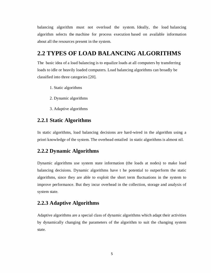
4. Microprocessor:

The function of the microprocessor are many like managing data collection,

performing power management and interfacing the system with the radio

layer.

5. Radio Transceiver :

The radio transceiver used in sending out messages into the network outside

in order to communicate properly.

6. Battery :

A lithium battery can be used in the working of the node to utilize as

minimum energy as possible.

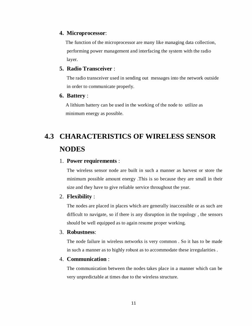
4.3 CHARACTERISTICS OF WIRELESS SENSOR

NODES

1. Power requirements :

The wireless sensor node are built in such a manner as harvest or store the

minimum possible amount energy .This is so because they are small in their

size and they have to give reliable service throughout the year.

2. Flexibility :

The nodes are placed in places which are generally inaccessible or as such are

difficult to navigate, so if there is any disruption in the topology , the sensors

should be well equipped as to again resume proper working.

3. Robustness:

The node failure in wireless networks is very common . So it has to be made

in such a manner as to highly robust as to accommodate these irregularities .

4. Communication :

The communication between the nodes takes place in a manner which can be

very unpredictable at times due to the wireless structure.

12

5. Cost and Size :

The nodes have to be made in small amount of money and size constraints are

also present

6. Large scale deployment :

The wireless sensor nodes are deployed in large numbers in order to get some

viable information regarding any phenomena, so the manufacturing should be

done keeping in mind so huge scalability and some degree of quality of

service.

4.4 SOFTWARE SUPPORT FOR WSN

The first operating system that came into prominence trying to meet specifically the

needs of wireless sensor networking is Tiny OS. Earlier some embedded operating

systems like µc/OS was thought of being used but it catered mostly to real time needs.

So, Tiny OS came into being with certain functionalities that were appropriate for this

only. Tiny OS is based on an event-driven programming model instead of multithreading.

Tiny OS programs are composed into event handlers and tasks with run to completion-

semantics. When an external event occurs, such as an incoming data packet or a sensor

reading, Tiny OS calls the appropriate event handler to handle the event.

4.5 WSN PROTOCOLS

1. IEEE 802.15.4

This standard was brought into picture specifically for the requirements of the

wireless sensor networks. This protocol supports multiple data rates and multiple

transmission frequencies .These have been referenced from [16].Its power

requirements are moderately low. Some of the important features are:

a. Transmission frequencies, 868 MHz/902–928 MHz/2.48–2.5 GHz.

b. Data rates of 20 Kbps (868 MHz Band) 40 Kbps (902 MHz band)

and 250Kbps (2.4 GHz band).

c. Supports star and peer-to-peer (mesh) network connections.

13

d. Standard specifies optional use of AES-128 security for encryption

of transmitted data.

2. ZIGBEE

The ZigBee Alliance[16] is an association of companies working together to

enable reliable, cost-effective, low-power, wirelessly networked monitoring

and control products based on an open global standard. The ZigBee alliance

specifies the IEEE 802.15.4 as the physical and MAC layer and is seeking to

standardize higher level applications such as lighting control and HVAC

monitoring.

3. 1451.5

While 802.15.4 [16] gives an insight into the communication architecture but it

falls short in the areas of specifying the sensor interface. The IEEE1451.5

wireless sensor working group aims to build on the efforts of previous IEEE1451

smart sensor working groups to standardize the interface of sensors to a wireless

network.

14

Chapter 5

RELATED WORKS

SOME EXISTING LOAD BALANCING MODELS

The following load balancing models have researched beforehand and all the facts

mentioned have been referenced from [1] and [2].

5.1 LOAD BALANCING IN STAR TOPOLOGY

SYSTEM MODEL DESCRIPTION

The network consists of one control processor and N communicating processors. It is

assumed that the total load is of arbitrarily divisible kind that can be partitioned into

fractions of loads to be assigned to processors over a network. The control processor first

assigns a load share to be measured to each of N processors and then receives the

measured data from each processor. Each processor begins to measure its share of load

once the measurement instructions from the controller have been received by each

processor [1].

The following 3 strategies have been used :

1. Simultaneous Measurement Start, Sequential Reporting

By a certain time , each processor will receive its measurement instructions from

the control processor . After the measurements are made, the model assumes only

one processor may report back to the root processor at a time. In this case the

processors receive their share of load from the root processor sequentially and start

computing after completely receiving their share of load.

2. Simultaneous Measurement Start, Simultaneous Reporting Termination

The network topology that is presented here is similar to above one barring one

fact that all the processors end their reporting time at the same time . For this to

happen , each processor needs a separate channel to the control processor.

15

3. Concurrent Measurement and Reporting

The model presented in this case is similar to above models except for the fact

that each processor has a co-processor that can measure and report at the same

time. Thus the moment the processor starts measuring data , it concurrently

reports the same to the control processor as well .

Studying the above models yields the conclusion that the last strategy minimizes the

reporting time the most and hence is the most efficient in nature.

5.2 LOAD BALANCING IN BUS NETWORKS

NETWORK MODEL

The bus interconnection topology is used in which the load is divisible and can be shared

among the different nodes. The processors are assumed to have uniform speeds . Closed

form and recursive equations can be derived using DLT to compute the minimum finish

time.

All the models mentioned here have been researched beforehand and have been

referenced from [2] .

1 . Bus Network With Control Processor

It consists of 1 control processor and other n communicating processor . The control

processor receives the measurement data and communicates it through a broadcast bus.

Each processor begins to compute its load once it gets the data.

2. No Control Processor, Processors With Front-End Processors

All the N processors have a front end processor with them . It implies that they can both

communicate and compute data at the same time. Hence the processor that originates the

load immediately starts computing as well as broadcasts its data to other processors. Each

processor starts computing data after receiving the load.

16

Chapter 6

LOAD BALACING USING D.L.T

6.1 NETWORK MODEL DESCRIPTION

The network topology considered in this case is a single level tree (star) topology

consisting of one control processor and n communicating processors. The following

assumptions have been made about the system model.

*The total load considered here is of the arbitrarily divisible kind that can be partitioned

into fractions of loads to be assigned to each processor over the network.

*Each processor begins to measure its share of load once the

controller allocates the share of load to be measured by

that processor.

*We also assume the computation time is negligible in

comparison to the allocation, measurement and reporting

time. Propagation delay is also ignored.

*Each communicating processor has a front end processor Fig 6.1 WSN (star topology)

for communication off-load.

6.2 STRATEGIES

The two newly proposed strategies for load balancing are

• Immediate measurement start and simultaneous reporting termination.

• Immediate measurement start and concurrent measurement and reporting.

17

Notations

αi- The fraction of load that is assigned to processor i by the control processor.

yi- A constant that is inversely proportional to the measuring speed of processor i

in the network.

zi- A constant that is inversely proportional to the communication speed of link i

in the network.

ai- A constant that is inversely proportional to the allocation speed of the link i of

the network.

Tms- Measurement intensity constant. This is the time it takes the ith processor to

measure the entire load when yi=1.The entire measurement load can be measured

on the ith processor in time yiTms.

Tcm- Communication intensity constant. This is the time it takes to transmit all of

the measurement load over a link when zi=1.The entire load can be transmitted

over the ith link in time ziTcm.

Tas- Alloocation intensity constant. This is the time it takes to allocate the entire

load α to the processor i when ai=1.

Ti- The total time that elapses between the beginning of the scheduling process at

t =0 and the time when processor i completes its reporting,

i=0, 1,..…,n. This includes allocation time, measurement time, reporting time and

idle time.

Tf- This is the time when the last processor finishes reporting (finish time).

Tf =max(T1,T2,…, Tn)

Some of the above used notations and parameters have been taken from [1] and

[2] .These parameters are already being used in finding the closed form equations

of load balancing in [1] and [2] for star and bus topologies.

18

6.2.1 Immediate Measurement Start, Simultaneous Reporting

Termination

In this strategy as soon as each processor receives its measurement instructions from the

control processor it starts measuring its load and it does not wait for the other processors

to receive their measurement instructions. It is assumed that processor receive their

measurement instructions in increasing order of their processor number. That is processor

i receives its measurement instructions first and is followed by processor i+1. It is

assumed that all the processors finish at the same time because the reporting time is

minimum if all the processors finish at the same time by sharing the load among

themselves. Both measurement and communication time have been considered.along

with the allocation time.

T1 = α1a1Tas + α1y1Tms+α1z1Tcm (1)

T2= (α1+α2)a2Tas+ α2y2Tms+α2z2Tcm (2)

...

Tn= (α1+α2 +…+αn )anTas + αn ynTms+ αnznTcm: (3)

For Tf to be minimum, T1=T2=…=Tn

α1(a1Tas+y1Tms+z1Tcm)= (α1 +α2 )a2Tas + α2y2Tms+ α2z2Tcm (4)

(α1+α2 )a2Tas+α2y2Tms+α2z2Tcm=(α1+α2+α3)a3Tas+α3y3Tms+α3z3Tcm (5)

….

(α1+α2+…+αn-1) an-1Tas+ αn-1yn-1Tms+αn-1zn-1

=(α1+α2+…+αn)anTas+αnynTms+αnznTcm (6)

Considering all nodes to be homogeneous, all yi , zi and ai are equal

Let, yiTms+ ziTcm=r

Let, aiTas=k

α1(k+r)= (α1+α2)k+ α2 r (7)

solving (7) we get, α2 = α1r/(k+r) (8)

Solving all the equations we get, αn = α1 rn-1

/(k+r)n-1

α1+ α2 +…+ αn =1 (as per DLT)

19

Let s= r/(k+r)

α1(1+s+s2+s

3+…+ s

n-1)=1 (9)

α1=(1-s)/(1-sn) (10)

αi= α1si-1

(11)

substituting value of α1 in T1 we get,

Tf = (aTas + yTms + zTcm)(1-s)/(1-sn)

As n approaches infinity, the expression (1-s)/(1-sn) approaches (1-s). Now using the

definition of s, one can easily obtain

(1-s)= k/(k+r)= aTas/(aTas+yTms+zTcm)

(12)

Tf =aTas (13)

From equation 11, we conclude that the load allocated to each processor will mainly

depend on the combined measurement and communication speed of that processor and to

an extent on the allocation speed of that processor.The lesser is the allocation time,the

more will be the load allocated.

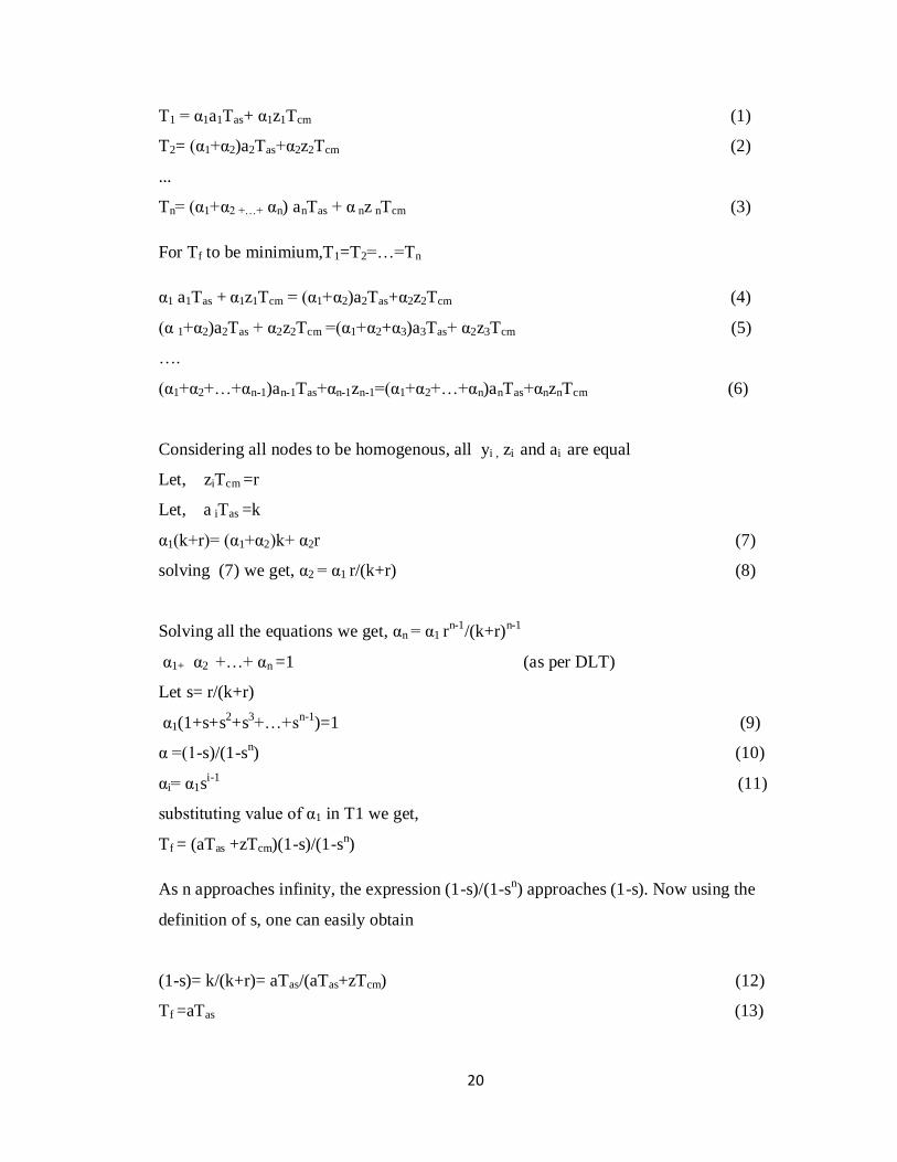
6.2.2 Immediate Measurement Start, Concurrent

Measurement and Reporting

In this strategy as soon as each processor receives its measurement instructions from the

control processor it starts measuring its load and it does not wait for the other processors

to receive their measurement instructions. It is assumed that processor receive their

measurement instructions in increasing order of their processor number. That is processor

i receives its measurement instructions first and is followed by processor i+1. It is

assumed that all the processors finish at the same time because the reporting time is

minimum if all the processors finish at the same time by sharing the load among

themselves. Only communication time and allocation time have been considered. Since it

is assumed that the measurement time is very less in comparison to the communication

time.

20

T1 = α1a1Tas+ α1z1Tcm (1)

T2= (α1+α2)a2Tas+α2z2Tcm (2)

...

Tn= (α1+α2 +…+ αn) anTas + α nz nTcm (3)

For Tf to be minimium,T1=T2=…=Tn

α1 a1Tas + α1z1Tcm = (α1+α2)a2Tas+α2z2Tcm (4)

(α 1+α2)a2Tas + α2z2Tcm =(α1+α2+α3)a3Tas+ α2z3Tcm (5)

….

(α1+α2+…+αn-1)an-1Tas+αn-1zn-1=(α1+α2+…+αn)anTas+αnznTcm (6)

Considering all nodes to be homogenous, all yi , zi and ai are equal

Let, ziTcm =r

Let, a iTas =k

α1(k+r)= (α1+α2)k+ α2r (7)

solving (7) we get, α2 = α1 r/(k+r) (8)

Solving all the equations we get, αn = α1 rn-1

/(k+r)n-1

α1+ α2 +…+ αn =1 (as per DLT)

Let s= r/(k+r)

α1(1+s+s2+s

3+…+s

n-1)=1 (9)

α =(1-s)/(1-sn) (10)

αi= α1si-1

(11)

substituting value of α1 in T1 we get,

Tf = (aTas +zTcm)(1-s)/(1-sn)

As n approaches infinity, the expression (1-s)/(1-sn) approaches (1-s). Now using the

definition of s, one can easily obtain

(1-s)= k/(k+r)= aTas/(aTas+zTcm) (12)

Tf =aTas (13)

21

Here in this case, the load allocated to each processor depends on communication speed

and mainly on allocation speed of that processor. As allocation speed decreases load

allocated to that processor increases.

So it can be seen that as the number of processor becomes infinity the final reporting time

becomes equal in both the cases. But in all other cases the immediate measurement and

concurrent reporting strategy is better than immediate measurement and simultaneous

reporting.

22

Chapter 7

RESULTS and ANALYSIS

The reporting time shown in the graphs are in milliseconds. For each strategy, the first

graph is the one obtained from the closed form equations and the second one is obtained

from the program.

7.1 STAR TOPOLOGY

For all graphs under this section, Tms=1,Tcm=1,y=1 and z is varied.

1. Simultaneous Measurement Start and Sequential Reporting

Fig 7.1.1 Simultaneous measurement start and sequential reporting

Fig 7.1.2 Simultaneous measurement start and sequential reporting

23

We see from the graphs shown above that as the number of processors increases the

reporting time decreases. After the number of processors becomes large the reporting

time becomes almost constant. Also as the constant zi increases the reporting time

increases since zi is inversely proportional to the communication speed of a link.

2. Simultaneous Measurement Start and Simultaneous Reporting

Fig 7.1.3 Simultaneous measurement start and simultaneous reporting

Fig 7.1.4 Simultaneous measurement start and simultaneous reporting

24

From the above graphs it is evident that the as the number of processors increases the

reporting time decreases. After the number of processors becomes sufficiently large the

reporting time becomes almost constant. The reporting time in this case is less than the

reporting time in case of sequential reporting. As zi increases the reporting time

increases.

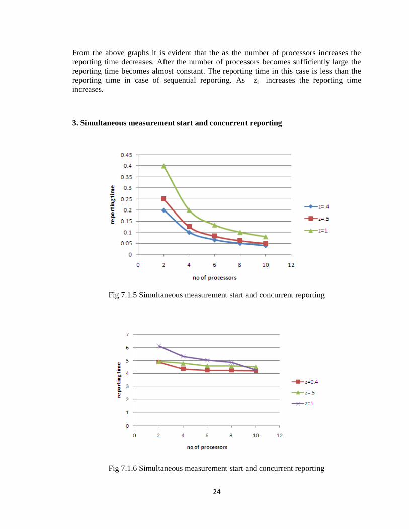
3. Simultaneous measurement start and concurrent reporting

Fig 7.1.5 Simultaneous measurement start and concurrent reporting

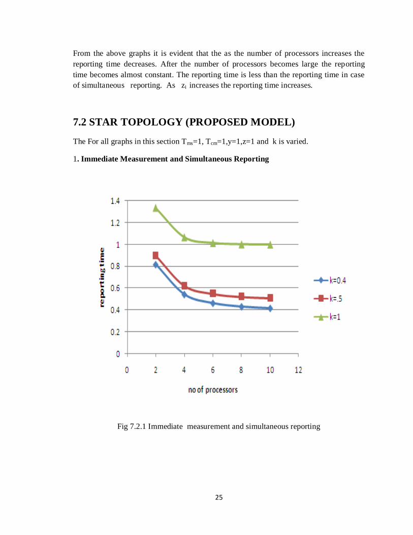
Fig 7.1.6 Simultaneous measurement start and concurrent reporting

25

From the above graphs it is evident that the as the number of processors increases the


time becomes almost constant. The reporting time is less than the reporting time in case

of simultaneous reporting. As zi increases the reporting time increases.

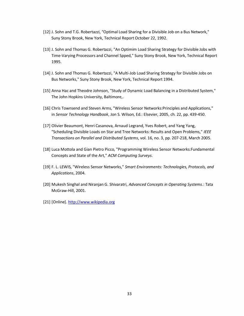
7.2 STAR TOPOLOGY (PROPOSED MODEL)

The For all graphs in this section Tms=1, Tcm=1,y=1,z=1 and k is varied.

1. Immediate Measurement and Simultaneous Reporting

Fig 7.2.1 Immediate measurement and simultaneous reporting

26

Fig 7.2.2 immediate measurement and simultaneous reporting

We see from the graph shown above that as the number of processors increases the


time becomes almost constant. Also as the constant ki increases the reporting time

increases since zi is inversely proportional to the allocation speed of a link.

2. Immediate Measurement Start and Concurrent Reporting

Fig 7.2.3 Immediate measurement start and concurrent reporting

27

Fig 7.2.4 Immediate measurement start and concurrent reporting

From the graph it is clear that as the number of processors increases the reporting time

decreases. Also the reporting time increases if ki increases because ki is inversely

proportional to the allocation constant The reporting time decreases nonlinearly upto

n=8 and then becomes almost constant.

28

7.3 BUS TOPOLOGY

For all graphs under this strategy .Tcp=1,Tcm=1,w=1 and z is varied.

1. Bus topology with a control processor

Fig 7.3.1 Bus topology with a control processor

Fig 7.3.2 Bus topology with a control processor



29


increases since zi is inversely proportional to the communication speed of a link. The

graph is steep in comparison to star topology and the reporting time is more in

comparison to star topology.

2. Bus topology without any control processor and with a front end processor

Fig 7.3.3 Bus topology without any control processor and processor with a front end

processor

Fig 7.3.4 Bus topology without any control processor and processor with a front end

processor

30




increases since zi is inversely proportional to the communication speed of a link. The

graph is steep in comparison to star topology and the reporting time is more in

comparison to star topology but less steep in comparison to the one in case of control

processor. The graph is more or less linear but actually it should become constant after

the number of processors becomes large. At z=0.4 the reporting time becomes constant

after some time.

31

Chapter 8

CONCLUSION

In this thesis, we have presented the problem of load balancing in wireless sensor

network using traditional divisible load theory. We extended an existing load balancing

approach which allocates load in a wireless sensor network connected in star topology. In

our proposed model we have considered the allocation time and found that the reporting

time is less in case of the strategy immediate measurement and concurrent reporting than

immediate measurement and simultaneous reporting. Among the existing strategies for

the star topology we have found from simulations that simultaneous measurement and

concurrent reporting has minimum reporting time. Among the two strategies considered

for bus topology the strategy no control processor and processors with frontend processor

has less reporting time. Also in the existing strategies if the allocation time is considered

then our proposed strategies has less reporting time.

Future Work

Load balancing being such a highly pivotal area of research in computer science , a lot of

improvement can be achieved in near future. It is expected that we could extend our study

and analysis to much varied range of sub topics like new hybrid topologies or incorporate

any other algorithm to improve the existing approaches.

32

Bibliography

[1] Mequanint Moges and Thomas G. Robertazzi, "Wireless Sensor Networks:Scheduling for

Measurement and Data Reporting," IEEE Transactions on Aerospace and Electronic Systems,

vol. 42, no. 1, pp. 327-340, January 2006.

[2] Sameer Bataineh, Te-Yu Hsiung, and Thomas G. Robertazzi, "Closed Form Solutions for Bus

and Tree Networks of Load Sharing a Divisible Load," IEEE Transactions on Computers, vol.

43, no. 10, pp. 1184-1196, october 1994.

[3] V. Mani and D. Ghose, "Distributed Computations in Linear Networks:Closed-Form

Solutions," IEEE Transactions on Aerospace and Electronic Systems, vol. 30, no. 2, pp. 471-

483, April 1994.

[4] Thomas G. Robertazzzi,Dantong Yu Mequanint A. Moges, "Divisible Load Scheduling with

Multiple Sources:Closed Form Solutions," in Conference on Information Sciences and

Systems, The Johns Hopkins University,Baltimore,Maryland, 2005.

[5] V., Ghose, D., and Robertazzi, T. G. Bharadwaj, "Divisible Load Theory: A New Paradigm for

Load Scheduling in," Cluster Computing, vol. 6, pp. 7-17, 2003.

[6] T. G. Robertazzi, "Ten reasons to use divisible load theory.," Computer, vol. 36, pp. 63-68,

2003.

[7] Li Guodong and Zhang Defu, "Distributing and Scheduling Divisible Task on Parallel

Communicating Processors," Journal of Computer Science and Technology, vol. 17, no. 6,

November 2002.

[8] M Lawenda and M. Drozdowski, "Scheduling multiple divisible loads in homogeneous star

systems," Journal of Scheduling, vol. 11, no. 5, pp. 347-356, October 2008.

[9] Veeravalli Bharadwaj, "Efficient Scheduling Strategies for Processing Multiple Divisible Loads

on Bus Networks," Journal of Parallel and Distributed Computing, vol. 62, no. 1, pp. 132-151,

January 2002.

[10] Justin E. Clareburt, "Effective Load Balancing Strategies in Distributed Systems," University of

Queensland,.

[11] Mark A. Perillo and Wendi B. Heinzelman, "Wireless Sensor Network Protocols," University

of Rochester, Rochester, NY, USA,.

33

[12] J. Sohn and T.G. Robertazzi, "Optimal Load Sharing for a Divisible Job on a Bus Network,"

Suny Stony Brook, New York, Technical Report October 22, 1992.

[13] J. Sohn and Thomas G. Robertazzi, "An Optimim Load Sharing Strategy for Divisible Jobs with

Time-Varying Processors and Channel Spped," Suny Stony Brook, New York, Technical Report

1995.

[14] J. Sohn and Thomas G. Robertazzi, "A Multi-Job Load Sharing Strategy for Divisible Jobs on

Bus Networks," Suny Stony Brook, New York, Technical Report 1994.

[15] Anna Hac and Theodre Johnson, "Study of Dynamic Load Balancing in a Distributed System,"

The John Hopkins University, Baltimore,.

[16] Chris Townsend and Steven Arms, "Wireless Sensor Networks:Principles and Applications,"

in Sensor Technology Handbook, Jon S. Wilson, Ed.: Elsevier, 2005, ch. 22, pp. 439-450.

[17] Olivier Beaumont, Henri Casanova, Arnaud Legrand, Yves Robert, and Yang Yang,

"Scheduling Divisible Loads on Star and Tree Networks: Results and Open Problems," IEEE

Transactions on Parallel and Distributed Systems, vol. 16, no. 3, pp. 207-218, March 2005.

[18] Luca Mottola and Gian Pietro Picco, "Programming Wireless Sensor Networks:Fundamental

Concepts and State of the Art," ACM Computing Surveys.

[19] F. L. LEWIS, "Wireless Sensor Networks," Smart Environments: Technologies, Protocols, and

Applications, 2004.

[20] Mukesh Singhal and Niranjan G. Shivaratri, Advanced Concepts in Operating Systems.: Tata

McGraw-Hill, 2001.

[21] [Online]. http://www.wikipedia.org

http://www.wikipedia.org/

Load Balancing in Wireless Sensor Network using Divisible...

Documents

Transcript of Load Balancing in Wireless Sensor Network using Divisible...