Y.Q. Shi, H.J. Kim, and F. Pérez-González (Eds.): IWDW 2012, LNCS 7809, pp. 368–383, 2013. © Springer-Verlag Berlin Heidelberg 2013

Optimal Histogram-Pair and Prediction-Error Based Image Reversible Data Hiding*

Guorong Xuan1, Xuefeng Tong1, Jianzhong Teng1, Xiaojie Zhang1, and Yun Qing. Shi2

1 Computer Science, Tongji University, Shanghai, China 2 ECE, New Jersey Institute of Technology, Newark, New Jersey, USA

grxuan@tongji.edu.cn, shi@njit.edu

Abstract. This proposed scheme reversibly embeds data into image prediction-errors by using histogram-pair method with the following four thresholds for optimal performance: embedding threshold, fluctuation threshold, left- and right-histogram shrinking thresholds. The embedding threshold is used to select only those prediction-errors, whose magnitude does not exceed this threshold, for possible reversible data hiding. The fluctuation threshold is used to select only those prediction-errors, whose associated neighbor fluctuation does not exceed this threshold, for possible reversible data hiding. The left- and right-histogram shrinking thresholds are used to possibly shrink histogram from the left and right, respectively, by a certain amount for reversible data hiding. Only when all of four thresholds are satisfied the reversible data hiding is carried out. Different from our previous work, the image gray level histogram shrinking towards the center is not only for avoiding underflow and/or overflow but also for optimum performance. The required bookkeeping data are embedded together with pure payload for original image recovery. The experimental results on four popularly utilized test images (Lena, Barbara, Baboon, Airplane) and one of the JPEG2000 test image (Woman, whose histogram does not have zero points in the whole range of gray levels, and has peaks at its both ends) have demonstrated that the proposed scheme outperforms recently published reversible image data hiding schemes in terms of the highest PSNR of marked image verses original image at given pure payloads.

Keywords: Reversible image data hiding, prediction error, neighborhood fluctuation, histogram pair scheme, gray level histogram modification.

1 Introduction

Reversibility requires that not only the hidden data can be extracted correctly but also the marked image can be inverted back to the original cover image exactly after the hidden data extraction. Research on reversible, also called lossless, image data hiding has attracted great interests recently, which can be manifested by the dramatically and

* This research is largely supported by Shanghai City Board of education scientific research

innovation projects (12ZZ033) and National Natural Science Foundation of China (NSFC) on project (90304017).

Optimal Histogram-Pair and Prediction-Error Based Image Reversible Data Hiding 369

continuously increasing number of publications on this subject, e.g., [1-14] (just a rather incomplete list). This is because reversible data hiding has found wide applications in image content authentication, e-banking and e-government, to name a few.

In the beginning stage, module 256 addition was used to achieve reversibility [1]. However, it has been realized that module 256 addition may damage image quality severely, and hence has been less used nowadays [15,16]. Lower bit-plane compression has shown to be able to fulfill reversible data hiding [2,3] with improved visual quality. The data embedding rate is however not high though. Note that when the data embedding is conducted in integer wavelet transform (IWT) domain [3], one or two sides of histogram of the image in which data is embedded may need to be shrunk towards the center (referred to as histogram modification) in order to keep reversibility. Difference expansion method [4] has largely boosted the amount of data that can be reversibly embedded. Histogram manipulation method [5] has demonstrated high quality of image with data losslessly embedded. Along this line, via quite some progressive improvements [e.g., 6,7], histogram-pair method [8] works on high frequency wavelet subbands further significantly improves lossless data embedding efficiency. Reversibly embedding data into prediction-error [9] is another effective scheme to largely boost embedding effectiveness in terms of the PSNR of the image with data hidden with respect to the original image versus data embedding rate. While many advanced reversible data hiding works [e.g., 10,11,12,13] have continued to appear in the literature, indicating this is a promising research subject for digital world; the work using sorting and prediction [13] may have provided generally the best performance in the literature at this stage.

In this paper, to achieve optimum performance (the highest PSNR at given capacity without overflow and/or underflow) we propose a scheme to reversibly embed data into image prediction-errors by using histogram-pair method with the following four thresholds: embedding threshold, fluctuation threshold, left- and right-histogram shrinking thresholds. The embedding threshold is used to select only those prediction-errors, whose magnitude does not exceed this threshold, for possible reversible data hiding. The fluctuation threshold is used to select only those prediction-errors, whose associated neighbor fluctuation does not exceed this threshold, for possible reversible data hiding. The left- and right-histogram shrinking thresholds are used to possibly shrink histogram from the left and/or right towards the center by a certain amount for reversible data hiding. An initial and short version of this framework was reported in [14], where only two thresholds were presented and without demonstration of how to achieve the optimality. Furthermore, in [14], the possible left- and/or right-histogram end shrinking is designed and conducted to only achieve reversibility, i.e., they have never been considered and manipulated to achieve the optimality in reversible data embedding. There are also some other minor differences between two schemes.

In order to facilitate the readers who may not know the principle of histogram-pair reversible data hiding [8] to follow this paper, a very simple example is presented here. In Fig. 1, the original image (9 pixels only) has 4 different pixel values: {6,7,8,9}. The to be embedded data are four bits: [1,0,0,1]. In Fig. 1 (a), the original image is shown, its histogram is [h(6),h(7),h(8),h(9)]=[4,3,1,1]. In Fig. 1 (b) histogram modification is made, i.e., a pixel with gray value 9 is changed to 8 in order to avoid overflow after data embedding. The information of this change needs to be

370 G. Xuan et al.

embedding into image as well so as to recover the original image exactly after the hidden data has been extracted. The histogram is hence changed to [h(6),h(7),h(8),h(9)]=[4,3,2,0]. In Fig. 2(c), a histogram-pair [h(6),h(7)]=[4,0] is created by change three pixels’ gray values from 7 to 8, and two gray values from 8 to 9. The histogram is thus changed to [h(6),h(7),h(8),h(9)]=[4,0,3,2]. The [4,0] is referred to as a histogram pair, which can be used for data embedding. In Fig. 2(d), four bits, [1,0,0,1] are embedded into this histogram-pair, that is, the histogram-pair [h(6),h(7)]=[4,0] changes to [h(6),h(7)]=[2,2]. That is, after four bits embedding, the histogram changes to [h(6),h(7),h(8),h(9)]=[2,2,3,2]. As said, during the embedding process the bookkeeping data need to be embedded into the image for the image recovery late and this detail is not shown here.

Fig. 1. Simple example of data hiding by histogram-pair (a) original image, (b) histogram modification, (c) creation of histogram-pair, (d) after data embedded

As shown above, because histogram shifting is used in data embedding which may lead to underflow and/or overflow, it is sometimes necessary for us to shrink one or two ends of image histogram towards the center. Note that some frequently used images, e.g., Lena, Barbara, and Airplane have two ends of their histogram being zero. However, Baboon image has its left-side of histogram non-zero, and Woman image, a JPEG2000 test image, has both sides of its histogram non-zero. Hence under these two circumstances it is necessary to shrink one-side or both sides of image histogram towards the center to reversibly embed data. Fig. 2 illustrates this procedure. Different from our previous work, where the image gray level histogram shrinking towards the center is conducted only for avoiding underflow and/or overflow, in this work how much to shrink the histogram also becomes two of four thresholds to seek optimal reversible data hiding.

(a) Original gray level histogram (b) Adjusted histogram (c) Histogram after data embedding

Fig. 2. Histogram modification in reversible data hiding

Optimal Histogram-Pair and Prediction-Error Based Image Reversible Data Hiding 371

The rest of the paper is organized as follows. The principle of four thresholds is presented in Section 2. The block diagram of the proposed scheme and a short example to illustrate the algorithm are shown in Section 3. In Section 4, experimental works on four popularly used test images and one of JPEG2000 test image are presented. In doing so, how to achieve optimality by using the proposed algorithm is demonstrated. The conclusion and discussion are made in Section 5.

2 Four Thresholds

In our work, a pixel, x, and its eight-neighbor, x1, x2, x3, x4, x5, x6, x7, x8, depicted in Eq. 1, are considered. The proposed method can also work with other types of neighbor, say, the four-neighbor. However, it can be shown that the eight-neighbor works more efficient than, say, the four-neighbor.

853

72

641

xxx

xxx

xxx (1)

The prediction error, PE, is defined as follows, where the prediction of the central pixel, x , is derived from its eight-neighbors.

xxPE −= ( )

+=

== 7,5,4,28,6,3,1

2121i

ii

i xxxwhere (2)

The fluctuation value, F, associated with the above-mentioned eight-neighbor, is defined as follows. That is, the related average value, x , is equal to the above-mentioned prediction of the central pixel. The fluctuation value depends on eight neighbor pixels values.

( ) ( ) ( )

−+−=

== 7,5,4,2

2

8,6,3,1

2 231i

ii

i xxxxF (3)

(1) Fluctuation threshold, TF

In this reversible data hiding algorithm, for each candidate pixel, we calculate the fluctuation using Eq. 3 from its surrounding 8-eighbors, and compare it with the fluctuation threshold TF. If the calculated fluctuation, F, is larger than or equal to the fluctuation threshold, TF, i.e., F ≥TF, the pixel is untouched. Only when the calculated fluctuation, F, is smaller than TF, a bit can possibly be embedded.

(2) Embedding threshold, T For a pixel under consideration, which has satisfied the fluctuation threshold, TF, it

may be selected to embed a bit, or it may be expanded without data embedding, or remaining non-touched at all, depending on the embedding threshold T.

Specifically, PE has the following three possible different situations. Let us consider PE ≥ 0 and T ≥ 0. First, PE = T, a bit of data will be embedded: PE = PE+b, b

372 G. Xuan et al.

is a bit that we want to be added at this time. Second, PE > T, we do not embed data, instead the PE is extended, i.e., PE = PE +1. Third, PE < T, do nothing. If PE < 0 and T< 0, similarly we have three different situations. All details are shown in Fig. 3.

(3) Right-histogram threshold, TR Right-histogram threshold is such a threshold that the gray level at right histogram

will be shrank by TR to make largest gray level become smaller than 255, prior to data embedding [8,14]. Different from [8,14], however, in this paper this threshold is adjusted not only to prevent underflow and/or overflow but also to achieve the optimal performance in reversible data hiding.

(4) Left-histogram threshold, TL Similarly, left-histogram threshold is such a threshold that the gray level at left

histogram will be shrank by TL to make the smallest gray level larger than 0 prior to data hiding. Here the TL is designed not only to prevent underflow but also to achieve the optimal performance in reversible data hiding.

3 Proposed Algorithm

In this section, we first present the principle of the proposed optimal algorithm, then the block diagrams of data embedding and retrieval, finally a simple example to illustrate the data hiding and extraction. To save the space, all of the formulae which have appeared in the block diagrams are not shown in the text again.

3.1 Proposed Optimal Algorithm

With the embedding threshold T, fluctuation threshold TF, left- and right-histogram adjustment thresholds TL and TR, under the constraints of no underflow and/or overflow, and the give embedding requirement, our proposed reversible data hiding scheme can be expressed as follows.

])([maxarg],,,[ PayloadPSNRTTTT

capacityembeddingmeetingoverflownorunderflowneither

RLF = (4)

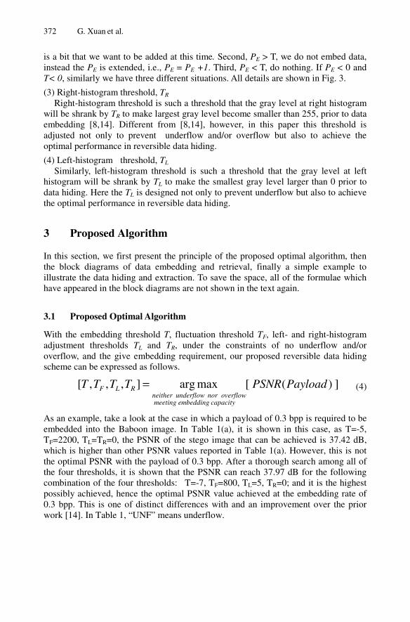
As an example, take a look at the case in which a payload of 0.3 bpp is required to be embedded into the Baboon image. In Table 1(a), it is shown in this case, as T=-5, TF=2200, TL=TR=0, the PSNR of the stego image that can be achieved is 37.42 dB, which is higher than other PSNR values reported in Table 1(a). However, this is not the optimal PSNR with the payload of 0.3 bpp. After a thorough search among all of the four thresholds, it is shown that the PSNR can reach 37.97 dB for the following combination of the four thresholds: T=-7, TF=800, TL=5, TR=0; and it is the highest possibly achieved, hence the optimal PSNR value achieved at the embedding rate of 0.3 bpp. This is one of distinct differences with and an improvement over the prior work [14]. In Table 1, “UNF” means underflow.

Optimal Histogram-Pair and Prediction-Error Based Image Reversible Data Hiding 373

Table 1. PSNR improvement by TL and TR for Baboon image

(a) Baboon at TL=0 (b) Baboon at TL=5

PSNR=37.42 ,paylaod=0.3, T=-5, TF=2200 at TL=0,TR=0 PSNR=37.97 ,paylaod=0.3, T=-7, TF=800 at TL=5,TR=0

T\TF 2000 2100 2200 2300 2400 T\TF 600 700 800 900 1000 -6 UNF UNF 37.17 37.11 37.07 -8 37.74 37.91 37.81 37.72 37.66 5 37.41 37.37 37.29 37.26 37.21 7 37.52 37.93 37.89 37.86 37.81 -5 37.34 37.42 37.42 37.38 37.36 -7 37.34 37.82 37.97 37.86 37.77 4 36.72 36.74 36.68 36.67 36.65 6 37.07 37.48 37.70 37.89 37.82 -4 UNF UNF UNF UNF UNF -6 36.78 37.19 37.49 37.62 37.72

3.2 Block Diagram

The block diagrams of data embedding and retrieval for the proposed algorithm are shown in Fig. 3 and Fig. 4, respectively.

Note that there is another difference between the proposed algorithms with that reported in [8,14]. That is, instead of from one-side of a histogram, say, T=4, to reversibly embed data, if the to-be embedded data have not been all embedded, the algorithm embeds data in T=-4, and so on, in this proposed algorithm, differently, we scan the image and embed data into both tP=4 as well as tN=-4 as the first step. If the data have not been completely embedded, we are to embed data to the next pair of

Fig. 3. Flowchart of data embedding

374 G. Xuan et al.

Fig. 4. Flowchart of data extracting of proposed scheme

tP=3 and tN=-3. That is, the data embedding in an order of {4,-4},{3,-3},{2,-2}, {1,-1},{0}. Note that it can also be: {-4,3},{-3,2},{-2,1},{-1,0}. Furthermore, depends on the situation, it is not necessary that the data embedding process has to end up at {0}, it can end at any value in the sequence prior to 0, e.g., it can end, respectively, at -4 and 3 in the two sequences listed above. As long as the required amount of data has been embedded, the algorithm stops. Our experimental results have demonstrated that this strategy can lead to a higher PSNR of a stego image versus the original image for the case where the pure payload (amount of data that needs to be embedded) is not large.

3.3 An Illustrative Example

For simplification, the fluctuation value F of a pixel under consideration in this example only depends on the four neighbors sounding this pixel.

Below, a simplified example is used to illustrate: 1) how data can be embedded into an original image to generate a stego image (the image with the data hidden inside); 2) how the hidden data can be extracted out without any error, and the stego image can turn back to the original image without any difference. In doing so, to simplify the procedure, we do not use 8-neighbor in prediction; instead, 4-neighbor is used in the demonstration. That is, Eq. (3) is now simplified as:

Optimal Histogram-Pair and Prediction-Error Based Image Reversible Data Hiding 375

154 158 160 158 160 162 162 154 158 160 158 160 162 162 158 158 159 160 160 159 162 158 158 159 160 160 159 162 153 158 157 159 161 162 162 153 158 157 159 161 162 162

(a) PE=0, F=1<4, emb data [1], PE=0→1 (j) End of extracting data [1,0]

154 158 160 158 160 162 162 154 158 160 158 160 162 162

158 159 159 160 160 159 162 158 159 159 160 160 159 162

153 158 157 159 161 162 162 153 158 157 159 161 162 162

(b) PE=0, F=6>4, no emb., PE=0→0 (i) PE=1, F=1<4, ext. data [1], PE=1→0

154 158 160 158 160 162 162 154 158 160 158 160 162 162

158 159 159 160 160 159 162 158 159 159 160 160 159 162

153 158 157 159 161 162 162 153 158 157 159 161 162 162

(c) PE=1, F=2<4, no emb. and expand, PE=1→2 (h) PE=0, F=6>4, no ext.,PE=0→0

154 158 160 158 160 162 162 154 158 160 158 160 162 162

158 159 159 161 160 159 162 158 159 159 161 160 159 162

153 158 157 159 161 162 162 153 158 157 159 161 162 162

(d) PE=0, F=3<4, emb. data [0], PE=0→0 (g) PE=2, F=2<4, no ext. and recover PE=2→1

154 158 160 158 160 162 162 154 158 160 158 160 162 162 158 159 159 161 160 159 162 158 159 159 161 160 159 162 153 158 157 159 161 162 162 153 158 157 159 161 162 162

(e) End of embedding. data [1,0] (f) PE=0, F=3<4, ext.data [0], PE=0→0

(A) Embedding from top(a) to bottom(e) (B) Exacting from bottom(f) to top(i)

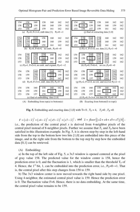
Fig. 5. Embedding and exacting data [1,0] with T= 0 , TF = 4, TL=0 , TR =0

( ) ( ) ( ) ( )2 2 2 22 4 5 7F x x x x x x x x= − + − + − + − , and ( ){ }2 4 5 7 4x floor x x x x= + + + ,

i.e., the prediction of the central pixel x is derived from 4-neighbor pixels of the central pixel instead of 8-neighbor pixels. Further we assume that TL and TR have been satisfied in this illustration example. In Fig. 5, it is shown step-by-step in the left-hand side from the top to the bottom how two bits [1,0] are embedded into this piece of the image, and in the right side from the bottom to the top step by step how the embedded data [0,1] can be retrieved.

(A) Embedding: a) In the top of the left side of Fig. 5, a 3x3 window is opened centered at the pixel

of gray value 158. The predicted value for the window center is 158, hence the prediction error is 0, and the fluctuation is 1, which is smaller than the threshold TF of 4. Hence, the 1st bit, 1, can be embedded into the prediction error, i.e., PE=0→1. That is, the central pixel after this step changes from 158 to 159.

b) The 3x3 window center is now moved towards the right hand side by one pixel. Using 4-neighbor, the estimated central pixel value is 159. Hence the prediction error is 0. The fluctuation value F=6. Hence, there is no data embedding. At the same time, the central pixel value remains to be 159.

376 G. Xuan et al.

c) Now the window center moves to the next pixel, whose gray value is 160 as shown in the sub-figure (c). Hence, the PE=1, F=2<4, no data embedding here, instead the PE is extended to 2, i.e., PE =1→2, thus making the central pixel gray value160161.

d) The window center moves to the following point 160 as in sub-figure (d). The prediction error PE=0, F=3<4, hence the 2nd bit, 0, is embedded, the central pixel remains to be 160. PE=0→0.

At this point two bits [1,0] have been embedded and the algorithm stop, as shown in sub-figure (e). The point becomes the end point.

(B) Extracting: The decoding starts from the ending point of data embedding, as shown in (f),

backwards to the starting point of data embedding in (j). Due to the space constraint, the detail in step-by-step has been omitted here.

One important observation is made here. That is, take a look at Fig. 5 (e) and Fig. 5 (f). All of 8 neighbor pixels in (d) are identical to all of 8 neighbor pixels in (f). Hence, the fluctuation value F in both cases are the same, and F=3. It can be observed that the eight neighbors in any specific 3x3 structure, hence the associated fluctuation F, during the data embedding is identical to the eight neighbors of a corresponding 3×3 structure in data extraction but in a reverse order. This is a key element to guarantee the reversibility.

Note that the procedure of embedding is fulfilled by a sequence of scanning the image gray level. Each scanning is scanned from the top-left to the bottom-right of an image.

4 Experimental Results

The results of applying the proposed algorithm to the following four frequently-utilized test images: Lena, Barbara, Airplane and Baboon [17] and one of the JPEG2000 test image Woman [18] have been reported in this section. It is observed that the first four test images have been widely utilized in reversible data hiding research community. It is observed that almost all of these four popularly used images have the two sides of their histograms empty (except the left side of Baboon image’s histogram), while their histograms are different from each other. On the other hand, it is noticed that the both ends of the histogram of Woman image have peaks. Therefore, it is recommended that the reversible data hiding community should pay attention to Woman image and test the proposed reversible data hiding algorithm on Woman image. In this section, we first present our test results on Woman image in detail. Afterwards, we present the summarized test results on the rest four test images.

Optimal Histogram-Pair and Prediction-Error Based Image Reversible Data Hiding 377

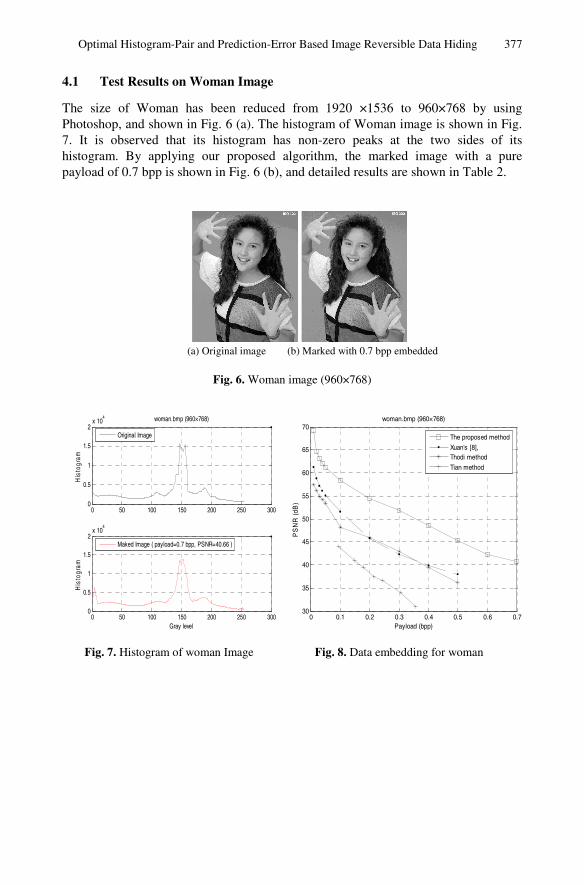
4.1 Test Results on Woman Image

The size of Woman has been reduced from 1920 ×1536 to 960×768 by using Photoshop, and shown in Fig. 6 (a). The histogram of Woman image is shown in Fig. 7. It is observed that its histogram has non-zero peaks at the two sides of its histogram. By applying our proposed algorithm, the marked image with a pure payload of 0.7 bpp is shown in Fig. 6 (b), and detailed results are shown in Table 2.

(a) Original image (b) Marked with 0.7 bpp embedded

Fig. 6. Woman image (960×768)

0 50 100 150 200 250 3000

0.5

1

1.5

2x 10

4

His

togr

am

woman.bmp (960×768)

Original Image

0 50 100 150 200 250 3000

0.5

1

1.5

2x 10

4

Gray level

His

togr

am

Maked Image ( payload=0.7 bpp, PSNR=40.66 )

0 0.1 0.2 0.3 0.4 0.5 0.6 0.730

35

40

45

50

55

60

65

70

Payload (bpp)

PS

NR

(dB

)

woman.bmp (960×768)

The proposed method

Xuan's [8],Thodi method

Tian method

Fig. 7. Histogram of woman Image Fig. 8. Data embedding for woman

378 G. Xuan et al.

Table 2. Data embedding into Woman image using the proposed method

Payload (bpp)

PSNR (dB)

T TF TL TR

Payload(bits)

(bpp×N)

Book- keeping

(bit) Cycle

Scan

Real payload

(bit) tN tP S

Time (sec)

0.01 69.22 -2 8 0 0 7372 0 1 1 7372 -2 1 -2 0 0.02 64.67 1 17 0 1 14745 1176 1 1 15921 -1 1 -1 1 0.03 63.15 0 6 0 1 22118 1176 1 1 23294 - 0 0 4 0.04 62.05 0 7 0 1 29491 1176 1 1 30667 - 0 0 8 0.05 61.18 0 7 0 1 36864 1176 1 1 38040 - 0 0 12 0.1 58.38 0 11 0 1 73728 1176 1 1 74904 - 0 0 19 0.2 54.35 1 50 1 1 147456 6327 1 1 153783 -1 1 -1 26

1 1 227468 -1 0 - 35 0.3 51.84 -1 130 1 1 221184 6327

2 1 43 -1 0 -1 35 1 100042 -2 1 - 45

0.4 48.70 -2 80 2 2 294912 12212 1 2 207082 -1 0 0 54 1 97183 -2 1 - 63

1 2 206323 -1 0 - 73 0.5 45.38 -2 60 3 3 368640 17826

2 1 82960 -2 1 1 81 1 119036 -2 1 - 90

1 2 231988 -1 0 - 100 0.6 42.34 -2 600 3 3 442368 17826

2 1 109170 -2 1 1 110 1 113211 -2 1 - 120

1 2 228200 -1 0 - 131 1 107204 -2 1 - 141

0.7 40.66 -2 300 4 4 516095 26849 2

2 94329 -1 0 -1 149

In Table 2, the tN, tP, which have been introduced in Section 3.2 and included in

Fig.3 and Fig.4, indicate specific threshold value the threshold T assumes at the left side and right side of the histogram of prediction-errors during the algorithm execution. The S stands for the stop point in data embedding, which is either the last tN or the last tP used in the algorithm. With the S and threshold T, the algorithm can retrieve data correctly. The “Time” listed in the right-most column of Table 2 is the time consumed in each case. Note that there are “Cycle” and “Scan” in Table 2. Take a look at the case of 0.5 bpp embedding. There are two cycles. In Cycle 1, there are two scans. In Scan 1, the first pair of {tN, tP} is equal to {-2, 1} and the second pair is {tN, tP}={-1, 0}. Since the required amount of data has not been completely embedded in Cycle 1 while the tP has reached 0, Cycle 2 embedding is conducted with {tN, tP}={-2,1}. Since 0.5 bpp has been embedded for the image, there is no need to another scan, and the algorithm stops. The real payload is the sum of payload and bookkeeping. The bookkeeping data are used to store the histogram modification information for data extracting and the original image recovery. For example, at 0.5 bpp case, the real payload is the payload, 368,640 bits, plus bookkeeping, 17,826 bits, equal to 386,466 bits. The real payload 386,466 can also be calculated through the circle and scan as 97183 (Circle 1, Scan 1) plus 206323 (Circle 1, Scan 2) and plus 82960 (Circle 2, Scan 1).

The performance comparison on the Waman iamge in terms of PSNR versus pure payload among our proposed method, and three prior-arts: Difference expansion method [4], Prediction-error expansion method [9], and Optimal histogram-pair based method [8] are shown in Fig. 8.

Optimal Histogram-Pair and Prediction-Error Based Image Reversible Data Hiding 379

PSNR=64.67,bpp=0.02,TL=0,TR=1 PSNR=64.67,bpp=0.02,T=1,TF=17

T\TF 11 14 17 20 23 TL\TR 4 0 1 2 3

2 UNF UNF Fail Fail Fail 4 50.06 OVF 50.34 50.3 50.22

-2 UNF UNF Fail Fail Fail 3 51.72 OVF 52.15 52.09 51.95

1 UNF UNF 64.67 64.65 64.62 0 Fail OVF 64.67 Fail Fail

-1 63.93 63.89 63.87 63.83 63.83 1 57.92 OVF 60.07 59.69 58.98

0 64.62 64.57 64.56 64.54 64.52 2 54.6 OVF 55.48 55.34 55.06

PSNR=62.05,bpp=0.04,TL=0,TR=1 PSNR=62.05,bpp=0.04,T=0,TF=7

T\TF 1 4 7 10 13 TL\TR 4 0 1 2 3

1 Fail UNF Fail Fail Fail 4 49.77 OVF 50.03 49.99 49.91

-1 Fail UNF Fail Fail Fail 3 51.4 OVF 51.78 51.72 51.61

0 Fail 62.01 62.05 61.97 61.88 0 59.1 OVF 62.05 61.49 60.47

-2 Fail UNF Fail Fail Fail 1 57.09 OVF 58.69 58.42 57.9

2 Fail UOF Fail Fail Fail 2 54.1 OVF 54.83 54.72 54.49

PSNR=58.38,bpp=0.1,TL=0,TR=1 PSNR=58.38,bpp=0.1,T=0,TF=11

T\TF 3 7 11 15 19 TL\TR 4 0 1 2 3

1 Fail UNF Fail Fail Fail 4 48.56 OVF OVF 48.78 48.69

-1 Fail UNF Fail Fail Fail 3 50.16 OVF OVF 50.54 50.38

0 Fail OVF 58.38 58.26 58.15 0 56.89 OVF 58.38 58.12 57.64

-2 Fail UOF Fail Fail Fail 1 54.96 OVF 56.58 56.25 55.64

2 Fail UOF UOF Fail Fail 2 52.46 OVF OVF 53.1 52.85

PSNR=51.84,bpp=0.3,TL=1,TR=1 PSNR=51.84,bpp=0.3,T=-1,TF=130

T\TF 110 120 130 140 150 TL\TR 4 0 1 2 3

-2 UOF UOF UOF UOF UOF 4 47.7 OVF OVF 47.88 47.81

1 OVF OVF OVF OVF OVF 0 Fail UOF Fail Fail Fail

-1 51.76 51.82 51.84 51.8 51.76 1 51.19 OVF 51.84 51.69 51.48

0 Fail Fail Fail Fail Fail 2 50.1 OVF OVF 50.44 50.31

2 UOF UOF UOF UOF UOF 3 48.76 OVF OVF 49 48.9

PSNR=45.38,bpp=0.5,TL=3,TR=3 PSNR=45.38,bpp=0.5,T=-2,TF=60

T\TF 20 40 60 80 100 TL\TR 1 2 3 4 5

-3 Fail UOF UOF UOF UOF 1 UOF UOF Fail Fail Fail

2 Fail UOF OVF OVF OVF 2 UOF UOF Fail Fail Fail

-2 Fail UOF 45.38 45.32 45.24 3 OVF OVF 45.38 45.31 45.23

1 Fail Fail OVF OVF OVF 4 OVF OVF 44.9 44.83 44.76

-1 Fail Fail Fail Fail Fail 5 OVF OVF 44.16 44.11 44.04

PSNR=40.66,bpp=0.7,TL=4,TR=4 PSNR=40.66,bpp=0.7,T=-2,TF=300

T\TF 100 200 300 400 500 TL\TR 2 3 4 5 6

-3 UOF UOF UOF UOF UOF 2 UOF UOF Fail Fail Fail

2 OVF OVF OVF OVF OVF 3 UOF UOF Fail Fail Fail

-2 Fail Fail 40.66 40.42 40.21 4 OVF OVF 40.66 40.64 40.59

1 Fail Fail Fail Fail Fail 5 OVF OVF 40.41 40.38 40.33

-1 Fail Fail Fail Fail Fail 6 OVF OVF 40.09 40.04 40.01

Table 3. Results of optimal thresholds T vs. TF (left), TL vs. TR (right) with different payload for Woman Image

380 G. Xuan et al.

In Table 3, the performance (PSNR at given data embedding rate) of optimal thresholds T vs. TF with some values of TL and TR (left), TL vs. TR with some values of T and TF (right) at different payload for Woman Image are listed. The sub-table of thresholds T vs. TF under fixed TL and TR are provided on the left. The sub-table of thresholds TL vs. TR under fixed T and TF are provided on the right. The highest PSNR of the stego image with respect to the original image in each sub-table has been indicated with a small box, from which one can observe the optimal “T and TF” or “TL and TR”. That is, the optimal embedding results for various embedding rate with all of four thresholds have been listed in Table 3 for the Woman image. There “UOF ” means both underflow and overflow, “UF” means underflow, “OF” means overflow, and “Fail” means embedding failure (i.e., the required amount of data cannot be embedded with the corresponding set of thresholds).

4.2 Test Results on Four Commonly Utilized Test Images

The curves of PSNR vs. payload for Lena, Barbara, Baboon and Airplane images are shown in Fig. 9 to Fig. 12, respectively.

4.3 Performance Summary on All of Five Test Image

The optimal thresholds utilized and the resultant PSNR achieved on the above-mentioned five test images by applying the proposed method with various data embedding rates ranging from 0.01 to 0.7 bpp are listed in Table 4, where, as said in Section 4.1, S is the stop value of the embedding threshold T. It is observed that as embedding rate is between 0.01 bpp and 0.7 bpp, TL and TR are all zero for Lena, Barbara and Airplane, meaning the optimality can be achieved as both TL and TR being zero for these payloads. It is sure if more data are embedded then the thresholds TL and TR will not be zero any more. For Woman and Baboon, however, the optimality often achieved with non-zero TL and TR even with the payload below 0.7 bpp because of their different histogram distribution, i.e., non-zero at both or one ends.

0 0.1 0.2 0.3 0.4 0.5 0.6 0.730

35

40

45

50

55

60

65

70

Payload (bpp)

PS

NR

(dB

)

Lena.bmp (512×512)

The proposed method

Sachnev method

Xuan's [8]Thodi method

Tian method

0 0.1 0.2 0.3 0.4 0.5 0.6 0.730

35

40

45

50

55

60

65

70

Payload (bpp)

PS

NR

(dB

)

barbara.bmp (512×512)

The proposed method

Sachnev method

Xuan's [8]Thodi method

Tian method

Fig. 9. Embedding for Lena Fig. 10. Embedding for Barbara

Optimal Histogram-Pair and Prediction-Error Based Image Reversible Data Hiding 381

0 0.1 0.2 0.3 0.4 0.5 0.6 0.725

30

35

40

45

50

55

60

65

Payload (bpp)

PS

NR

(dB

)

baboon.bmp (512×512)

The proposed method

Sachnev method

Xuan's [8]Thodi method

Tian method

0 0.1 0.2 0.3 0.4 0.5 0.6 0.735

40

45

50

55

60

65

70

Payload (bpp)

PS

NR

(dB

)

airplane.bmp (512×512)

The proposed method

Sachnev methodThodi P3

Thodi D3

Fig. 11. Embedding for Baboon Fig. 12. Embedding for Airplane

Table 4. PSNR and optimal thresholds on five test images with different payloads

Womanbpp 0.01 0.02 0.03 0.04 0.05 0.1 0.2 0.3 0.4 0.5 0.6 0.7

PSNR 69.22 64.67 63.15 62.05 61.18 58.38 54.35 51.84 48.70 45.38 42.34 40.66 T -2 1 0 0 0 0 1 -1 -2 -2 -2 -2 TF 8 17 6 7 7 11 50 130 80 60 600 300 TL 0 0 0 0 0 0 1 1 2 3 3 4 TR 0 1 1 1 1 1 1 1 2 3 3 4 S -2 -1 0 0 0 0 -1 -1 0 1 1 -1

Lenabpp 0.01 0.02 0.03 0.04 0.05 0.1 0.2 0.3 0.4 0.5 0.6 0.7

PSNR 67.08 63.78 61.79 60.38 59.22 55.44 50.87 47.29 45.16 43.18 41.47 39.89 T -4 4 3 -4 3 2 -1 2 -2 -3 -4 -5 TF 14 26 21 36 32 48 100 100 250 200 250 550 TL 0 0 0 0 0 0 0 0 0 0 0 0 TR 0 0 0 0 0 0 0 0 0 0 0 0 S -4 4 -3 -3 -2 -2 0 1 0 -1 3 -1

Barbarabpp 0.01 0.02 0.03 0.04 0.05 0.1 0.2 0.3 0.4 0.5 0.6 0.7

PSNR 68.28 64.89 62.76 61.19 60.04 55.97 50.50 47.07 44.67 42.32 39.57 37.40 T -4 -4 -4 -3 -3 2 -3 -3 -4 -6 -6 -6 TF 18 30 38 23 31 65 85 100 120 250 320 250 TL 0 0 0 0 0 0 0 0 0 0 0 0 TR 0 0 0 0 0 0 0 0 4 2 3 0 S 3 3 -4 -3 2 -2 1 -1 -1 -1 -5 2

Baboonbpp 0.01 0.02 0.03 0.04 0.05 0.1 0.2 0.3 0.4 0.5 0.6 0.7

PSNR 63.51 59.57 57.29 55.46 53.75 47.65 41.60 37.99 35.01 32.29 29.46 27.44 T -5 3 3 3 -3 -3 -4 -7 -11 -12 -13 -13 TF 85 110 180 310 510 540 660 800 1100 2400 2200 2400 TL 0 0 0 0 0 0 0 4 7 9 17 22 TR 0 0 0 0 0 0 0 0 0 0 15 0 S -5 3 3 3 2 1 -1 -1 0 0 8 4

Airplanebpp 0.01 0.02 0.03 0.04 0.05 0.1 0.2 0.3 0.4 0.5 0.6 0.7

PSNR 69.58 66.31 64.57 62.83 61.91 58.25 54.28 50.99 48.86 46.76 44.90 42.95 T 1 1 1 1 1 1 -1 1 -2 -3 -4 -5 TF 3 4 4 6 6 10 17 26 37 52 94 220 TL 0 0 0 0 0 0 0 0 0 3 0 4 TR 0 0 0 0 0 0 0 0 0 0 0 1 S -1 -1 1 1 -1 1 -1 0 -1 -3 -1 4

382 G. Xuan et al.

5 Discussion and Conclusion

The research on reversible data hiding has made rapid progress in the past decade. An optimal histogram-pair and prediction-error based method has been reported in the paper. Instead of based on two thresholds [8,14], i.e., embedding threshold T and fluctuation threshold TF, the four thresholds have been utilized in this new algorithm. That is, the left- and right-histogram shrinking parameters used in [6,7,8,14] have now become two additional thresholds, i.e., the left- and right-shrinking thresholds, respectively, in this proposed algorithm. They are adjusted not only to avoid overflow and/or underflow but also for optimal performance in reversible data embedding. The performance of this proposed algorithm has been further enhanced, in particular for Woman image, which is a JPEG2000 test image, whose histogram has peaks on both of its right and left ends. On this Woman image, the proposed scheme achieves 2.22dB, 3.35dB and 3.62dB higher PSNR at the embedding rates of 0.01 bpp, 0.1 bpp and 0.5 bpp, respectively, compared with what reported in [14]. Since the proposed algorithm works on prediction-error image, its performance is much higher than what reported in [8]. Another advancement made in this paper over [8,14] is that the optimization has been concretely conducted and demonstrated in this paper for the first time. That is, the optimality has been mentioned in [8,14], but there have been no concrete procedures.

One observation is made here. That is, in addition to Lena image, whose histogram has its two ends widely empty, we suggest that Woman image with both sides of its histogram having peaks should be added as a test image for the reversible data hiding community in reporting and comparing the performance of various reversible data hiding algorithms.

Compared with the state-of-the-art reversible data hiding scheme [4][9][13] whose embedding strategy can be represented by 2PE+b, where PE stands for error or prediction-error and b stands for the bit to be embedded, our histogram-pair based scheme is in spirit of PE+b. The performance comparison reported in this paper indicates that the strategy of PE+b is more efficient then 2PE+b in terms of the PSNR verses data embedding rate. Specifically, compared with Sachnev et al.’s method [13], perhaps the most advanced scheme reported in the literature, on 12 different payloads ranging from 0.01 bpp to 0.7 bpp, our proposed scheme has achieved on average 1.94 dB improvement for Lena image, 2.33 dB for Barbara image, 1.28 dB for Baboon image, and 1.01 dB for Airplane image.

Note that Ni et al.’s method [5] is the first method that uses the PE+b approach and image histogram shifting. There is no, however, consideration and procedure for achieving the optimality in terms of the PSNR of stego image versus data embedding rate. In terms of performance, the proposed method has been far more advanced than what reported by the method [5].

References

1. Honsinger, C.W., Jones, P., Rabbani, M., Stoffel, J.C.: Lossless recovery of an original image containing embedded data. US Patent: 6,278,791 (2001)

2. Fridrich, J., Goljan, M., Du, R.: Invertible authentication. In: Proc. SPIE Photonics West, Security and Watermarking of Multimedia Contents III, San Jose, California, vol. 397, pp. 197–208 (January 2001)

Optimal Histogram-Pair and Prediction-Error Based Image Reversible Data Hiding 383

3. Xuan, G., Zhu, J., Chen, J., Shi, Y.Q., Ni, Z., Su, W.: Distortionless data hiding based on integer wavelet transform. IEE Electronics Letters 38(25), 1646–1648 (2002)

4. Tian, J.: Reversible data embedding using a difference expansion. IEEE Transaction on Circuits and Systems for Video Technology 13(8), 890–896 (2003)

5. Ni, Z., Shi, Y.Q., Ansari, N., Su, W.: Reversible data hiding. In: Proceedings of IEEE International Symposium on Circuits and Systems (ISCAS), Bangkok, Thailand, vol. 2, pp. 912–915 (May 2003); Also appear in Ni, Z., Shi, Y. Q., Ansari, N., Su, W.: Reversible data hiding. IEEE Transactions on Circuits and Systems for Video Technology 16(3), 354-362 (2006)

6. Xuan, G., Shi, Y.Q., Yang, C., Zheng, Y., Zou, D., Chai, P.: Lossless data hiding using integer wavelet transform and threshold embedding technique. In: IEEE International Conference on Multimedia and Expo (ICME 2005), Amsterdam, Netherlands (July 2005)

7. Xuan, G., Yao, Q., Yang, C., Gao, J., Chai, P., Shi, Y.Q., Ni, Z.: Lossless data hiding using histogram shifting method based on integer wavelets. In: Shi, Y.Q., Jeon, B. (eds.) IWDW 2006. LNCS, vol. 4283, pp. 323–332. Springer, Heidelberg (2006)

8. Xuan, G., Shi, Y.Q., Chai, P., Cui, X., Ni, Z., Tong, X.: Optimum histogram pair based image lossless data embedding. In: Shi, Y.Q., Kim, H.-J., Katzenbeisser, S. (eds.) IWDW 2007. LNCS, vol. 5041, pp. 264–278. Springer, Heidelberg (2008)

9. Thodi, D.M., Rodríguez, J.J.: Reversible watermarking by prediction-error expansion. In: Proceedings of 6th IEEE Southwest Symposium on Image Analysis and Interpretation, Lake Tahoe, CA,USA, March 28-30, pp. 21–25 (2004); Also appear as Thodi, D.M., Rodriguez, J.J.: Expansion embedding techniques for reversible watermarking. IEEE Trans. Image Process 16(3), 721–730 (2007)

10. Kamstra, L., Heijmans, H.J.A.M.: Reversible data embedding into images using wavelet techniques and sorting. IEEE Transactions on Image Processing 14(12), 2082–2090 (2005)

11. Coltuc, D., Chassery, J.M.: Very fast watermarking by reversible contrast mapping. IEEE Signal Processing Letters 14(4), 255–258 (2007)

12. Lee, S., Yoo, C.D., Kalker, T.: Reversible image watermarking based on integer-to-integer wavelet transform. IEEE Transactions on Information Forensics and Security 2(3), pt. 1, 321–330 (2007)

13. Sachnev, V., Kim, H.J., Nam, J., Suresh, S., Shi, Y.Q.: Reversible watermarking algorithm using sorting and prediction. IEEE Transactions on Circuits and Systems for Video Technology 19(7), 989–999 (2009)

14. Xuan, G., Shi, Y.Q., Teng, J., Tong, X., Chai, P.: Double-threshold reversible data hiding. In: IEEE International Symposium on Circuits and Systems (ISCAS 2010), Paris, France (May 2010); Also appear in Xuan, G., Shi, Y.Q., Chai, P., Teng, J., Ni, Z., Tong, X.: Optimum histogram pair based image lossless data embedding. In: Shi, Y.Q. (ed.) Transactions on DHMS IV. LNCS, vol. 5510, pp. 84–102. Springer, Heidelberg (2009)

15. Shi, Y.Q.: Reversible data hiding. In: Cox, I., Kalker, T., Lee, H.-K. (eds.) IWDW 2004. LNCS, vol. 3304, pp. 1–12. Springer, Heidelberg (2005)

16. Ni, Z., Ni, Z., Shi, Y.Q., Ansari, N., Su, W., Sun, Q., Lin, X.: Robust lossless image data hiding designed for semi-fragile image authentication. IEEE Transactions on Circuits and Systems for Video Technology 18(4), 497–509 (2008)

17. http://sipi.usc.edu/database 18. Source JPEG2000 (JPSEC), ISO/IEC 15444-8 (April 2007)