Deriving Statistical Significance Maps

for SVM Based Image Classificationand Group Comparisons

Bilwaj Gaonkar and Christos Davatzikos

Section for Biomedical Image Analysis,University of Pennsylvania, Philadelphia, PA 19104, USA

Abstract. Population based pattern analysis and classification forquantifying structural and functional differences between diverse groupshas been shown to be a powerful tool for the study of a number ofdiseases, and is quite commonly used especially in neuroimaging. Thealternative to these pattern analysis methods, namely mass univariatemethods such as voxel based analysis and all related methods, cannot de-tect multivariate patterns associated with group differences, and are notparticularly suitable for developing individual-based diagnostic and prog-nostic biomarkers. A commonly used pattern analysis tool is the supportvector machine (SVM). Unlike univariate statistical frameworks for mor-phometry, analytical tools for statistical inference are unavailable for theSVM. In this paper, we show that null distributions ordinarily obtainedby permutation tests using SVMs can be analytically approximated fromthe data. The analytical computation takes a small fraction of the timeit takes to do an actual permutation test, thereby rendering it possibleto quickly create statistical significance maps derived from SVMs. Suchmaps are critical for understanding imaging patterns of group differencesand interpreting which anatomical regions are important in determiningthe classifier’s decision.

1 Significance

Precise quantification of group differences using medical images central in scien-tific studies of the effects of disease on the human body. The dominant approachaddressing this problem involves performing independent statistical testing ei-ther pixel/voxel-wise [1] or regions of interest (ROI-wise) in the image. It hasbeen argued that such univariate analysis might miss group difference patternsthat span multiple voxels or regions [2]. Hence, replacing univariate methods bymultivariate methods such as SVMs [3] [4][5] has been discussed in literature.However, unlike univariate methods [1], SVMs do not naturally provide statis-tical tests (and corresponding p-values) associated with every voxel/region ofan image. Permutation testing has been suggested for interpreting SVM out-put for such high dimensional data [6]. However, performing these tests is timeconsuming and computationally costly. Hence, we developed and validated ananalytical approximation for SVM permutation tests that allows for tremendous

N. Ayache et al. (Eds.): MICCAI 2012, Part I, LNCS 7510, pp. 723–730, 2012.c© Springer-Verlag Berlin Heidelberg 2012

724 B. Gaonkar and C. Davatzikos

computational speed up. Section 2 of this mauscript presents the theory thatallows us to achieve this speed up. Section 3 presents experiments that validatethe theory. Section 4 presents a brief discussion and possible avenues for furtherdevelopment.

2 Analysis

2.1 Support Vector Machines: Background

The support vector machine [7] is a powerful pattern classification engine thatwas first proposed in the nineties. In medical imaging it has been used to distin-guish cognitively abnormal people from controls based on their brain MR images.For completeness we briefly explain the concept of the SVM next. To use SVMswe stack preprocessed image data into a large rectangular matrix X ∈ Rm×p

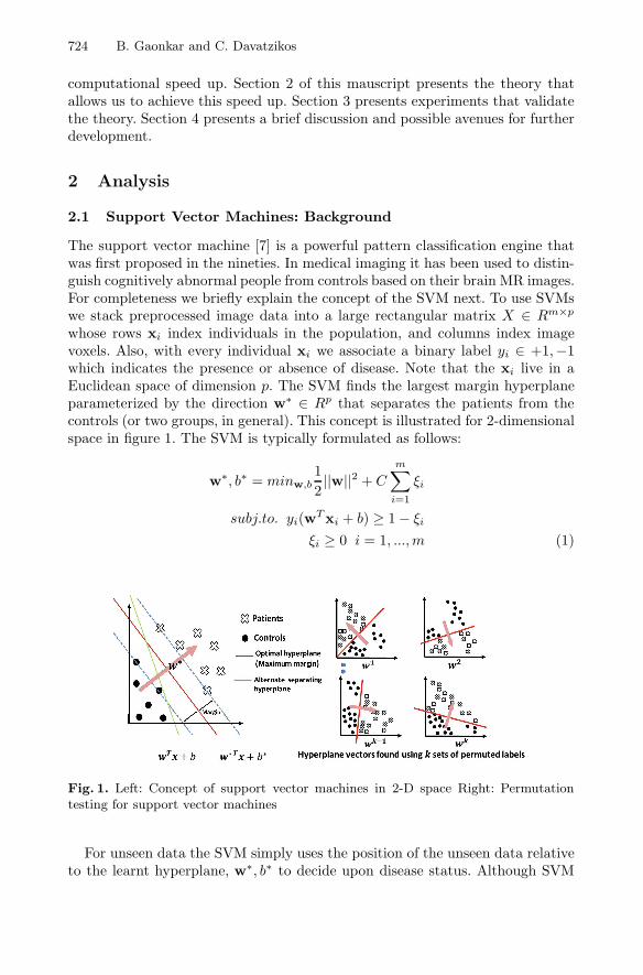
whose rows xi index individuals in the population, and columns index imagevoxels. Also, with every individual xi we associate a binary label yi ∈ +1,−1which indicates the presence or absence of disease. Note that the xi live in aEuclidean space of dimension p. The SVM finds the largest margin hyperplaneparameterized by the direction w∗ ∈ Rp that separates the patients from thecontrols (or two groups, in general). This concept is illustrated for 2-dimensionalspace in figure 1. The SVM is typically formulated as follows:

w∗, b∗ = minw,b1

2||w||2 + C

m∑

i=1

ξi

subj.to. yi(wTxi + b) ≥ 1− ξi

ξi ≥ 0 i = 1, ...,m (1)

Fig. 1. Left: Concept of support vector machines in 2-D space Right: Permutationtesting for support vector machines

For unseen data the SVM simply uses the position of the unseen data relativeto the learnt hyperplane, w∗, b∗ to decide upon disease status. Although SVM

Deriving Statistical Significance Maps for SVM 725

performance can be assessed by cross validation, it is equally important to beable to interpret which regions/features are important in deriving the classifier’sdecision. Such interpretations are particularly desirable by clinicians interestedin understanding how disease affects anatomy and function and which featuresthey should be attending to in interpreting medical images. Currently the onlyway to quantify importance of individual voxels to the SVM classification isthrough the use of permutation tests. The concept of permutation testing isillustrated in figure 1. Briefly, the data labels yi are permuted randomly. Foreach random permutation an SVM is trained and a hyperplane w is found. Aftermany permutations we can generate an approximation to the null distributionof each component of w. Comparing the components of w∗ with these nulldistributions allows for statistical inference. The inference procedure describedabove is based on [6]. Permutation testing is computationally expensive andbecomes increasingly difficult as dataset size increases. In this paper we developan analytical approximation of permutation testing using SVMs for medicalimaging data.

2.2 The Analytical Approximation of Permutation Testing forSVMs

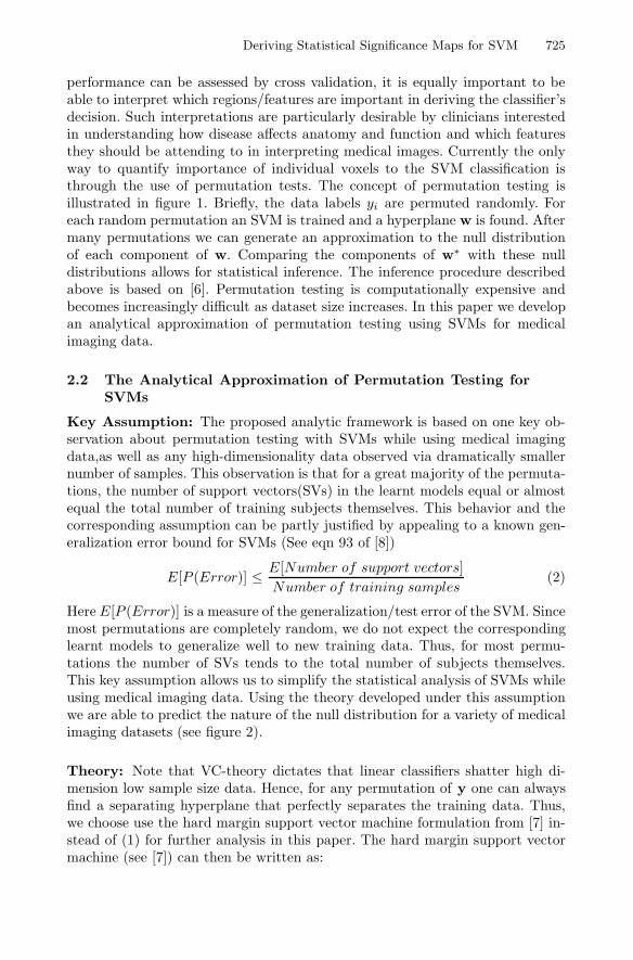
Key Assumption: The proposed analytic framework is based on one key ob-servation about permutation testing with SVMs while using medical imagingdata,as well as any high-dimensionality data observed via dramatically smallernumber of samples. This observation is that for a great majority of the permuta-tions, the number of support vectors(SVs) in the learnt models equal or almostequal the total number of training subjects themselves. This behavior and thecorresponding assumption can be partly justified by appealing to a known gen-eralization error bound for SVMs (See eqn 93 of [8])

E[P (Error)] ≤ E[Number of support vectors]

Number of training samples(2)

Here E[P (Error)] is a measure of the generalization/test error of the SVM. Sincemost permutations are completely random, we do not expect the correspondinglearnt models to generalize well to new training data. Thus, for most permu-tations the number of SVs tends to the total number of subjects themselves.This key assumption allows us to simplify the statistical analysis of SVMs whileusing medical imaging data. Using the theory developed under this assumptionwe are able to predict the nature of the null distribution for a variety of medicalimaging datasets (see figure 2).

Theory: Note that VC-theory dictates that linear classifiers shatter high di-mension low sample size data. Hence, for any permutation of y one can alwaysfind a separating hyperplane that perfectly separates the training data. Thus,we choose use the hard margin support vector machine formulation from [7] in-stead of (1) for further analysis in this paper. The hard margin support vectormachine (see [7]) can then be written as:

726 B. Gaonkar and C. Davatzikos

Fig. 2. For most permutations the number of support vectors in the learnt model isalmost equal to the total number of samples (a) simulated dataset(b) real datasetwith Alzheimer’s patients and controls (c) real dataset with schizophrenia patients andcontrols

Fig. 3. Experimental(blue histogram) and theoretically predicted(red line) null distri-butions for two randomly chosen components of w in (a) real dataset with Alzheimer’spatients and controls (b) simulated data

minw,b1

2||w||2

subj.to. yi(wTxi + b) ≥ 1 ∀i ∈ {1, ....,m}

It is required (see [9]) that for the ’support vectors’ (indexed by j ∈ {1, 2, .., nSV )we have wTxj+b = yj ∀j. Now, if all our data were support vectors this wouldallow us to write the constraints in optimization (3) as Xw + Jb = y where J isa column matrix of ones and X is a super long matrix with each row representingone image. Since this is indeed the case for most of our permutation tests (figure2), the optimization (3) becomes:

minw,b||w||2subj.to. Xw + Jb = y (3)

Deriving Statistical Significance Maps for SVM 727

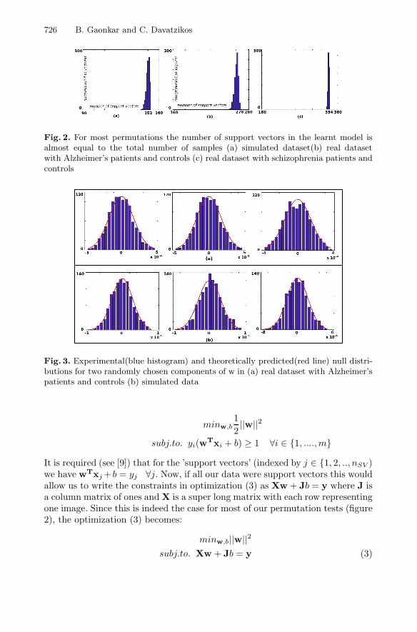
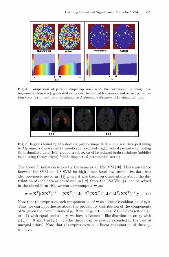
Fig. 4. Comparison of p-value maps(top row) with the corresponding image his-tograms(bottom row), generated using our theoretical framework and actual permuta-tion tests (a) In real data pertaining to Alzheimer’s disease (b) In simulated data

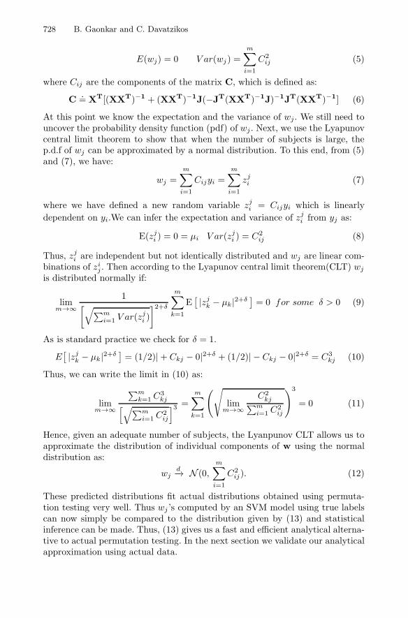
Fig. 5. Regions found by thresholding p-value maps at 0.05 a)in real data pertainingto Alzheimer’s disease (left) theoretically predicted (right) actual permutation testing(b)in simulated data (left) ground truth region of introduced brain shrinkage (middle)found using theory (right) found using actual permutation testing

The above formulation is exactly the same as an LS-SVM [10]. This equivalencebetween the SVM and LS-SVM for high dimensional low sample size data wasalso previously noted in [11] where it was based on observations about the dis-tribution of such data as elucidated in [12]. Since the LS-SVM, (4) can be solvedin the closed form [10], we can now compute w as:

w = XT[(XXT)−1 + (XXT)−1J(−JT(XXT)−1J)−1JT(XXT)−1]y (4)

Note that this expresses each component wj of w as a linear combination of yj ’s.Thus, we can hypothesize about the probability distribution of the componentsof w, given the distributions of yj . If we let yj attain any of the labels (either +1or −1) with equal probability, we have a Bernoulli like distribution on yj withE(yj) = 0 and V ar(yj) = 1 (the theory can be readily extended in the case ofunequal priors). Note that (5) expresses w as a linear combination of these yjwe have:

728 B. Gaonkar and C. Davatzikos

E(wj) = 0 V ar(wj) =

m∑

i=1

C2ij (5)

where Cij are the components of the matrix C, which is defined as:

C.= XT[(XXT)−1 + (XXT)−1J(−JT(XXT)−1J)−1JT(XXT)−1] (6)

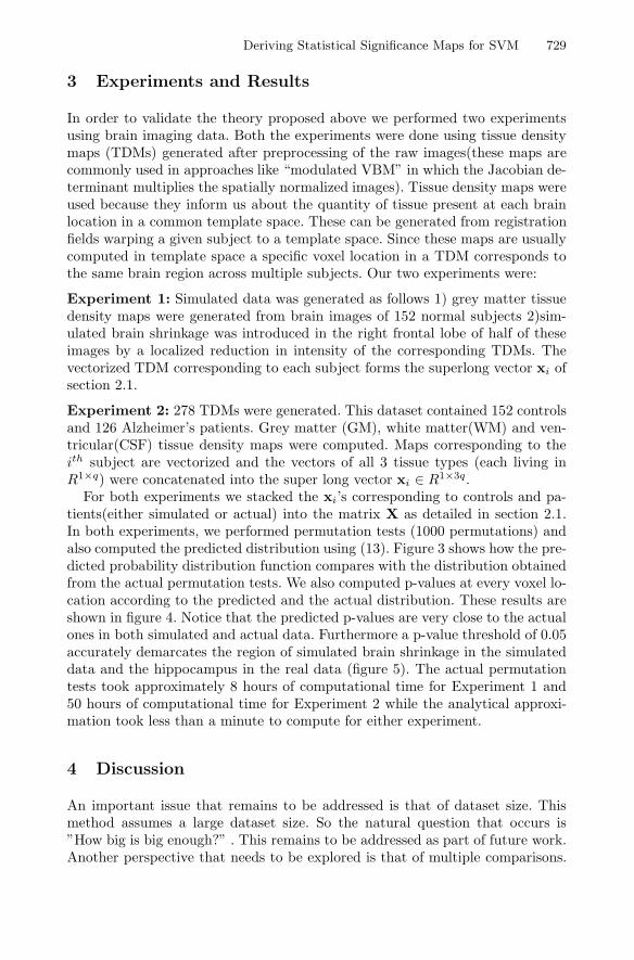
At this point we know the expectation and the variance of wj . We still need touncover the probability density function (pdf) of wj . Next, we use the Lyapunovcentral limit theorem to show that when the number of subjects is large, thep.d.f of wj can be approximated by a normal distribution. To this end, from (5)and (7), we have:

wj =

m∑

i=1

Cijyi =

m∑

i=1

zji (7)

where we have defined a new random variable zji = Cijyi which is linearly

dependent on yi.We can infer the expectation and variance of zji from yj as:

E(zji ) = 0 = μi V ar(zji ) = C2ij (8)

Thus, zji are independent but not identically distributed and wj are linear com-binations of zij . Then according to the Lyapunov central limit theorem(CLT) wj

is distributed normally if:

limm→∞

1[√∑m

i=1 V ar(zji )

]2+δ

m∑

k=1

E[ |zjk − μk|2+δ

]= 0 for some δ > 0 (9)

As is standard practice we check for δ = 1.

E[ |zjk − μk|2+δ

]= (1/2)|+ Ckj − 0|2+δ + (1/2)| − Ckj − 0|2+δ = C3

kj (10)

Thus, we can write the limit in (10) as:

limm→∞

∑mk=1 C

3kj[√∑m

i=1 C2ij

]3 =

m∑

k=1

(√

limm→∞

C2kj∑m

i=1 C2ij

)3

= 0 (11)

Hence, given an adequate number of subjects, the Lyanpunov CLT allows us toapproximate the distribution of individual components of w using the normaldistribution as:

wjd−→ N (0,

m∑

i=1

C2ij). (12)

These predicted distributions fit actual distributions obtained using permuta-tion testing very well. Thus wj ’s computed by an SVM model using true labelscan now simply be compared to the distribution given by (13) and statisticalinference can be made. Thus, (13) gives us a fast and efficient analytical alterna-tive to actual permutation testing. In the next section we validate our analyticalapproximation using actual data.

Deriving Statistical Significance Maps for SVM 729

3 Experiments and Results

In order to validate the theory proposed above we performed two experimentsusing brain imaging data. Both the experiments were done using tissue densitymaps (TDMs) generated after preprocessing of the raw images(these maps arecommonly used in approaches like “modulated VBM” in which the Jacobian de-terminant multiplies the spatially normalized images). Tissue density maps wereused because they inform us about the quantity of tissue present at each brainlocation in a common template space. These can be generated from registrationfields warping a given subject to a template space. Since these maps are usuallycomputed in template space a specific voxel location in a TDM corresponds tothe same brain region across multiple subjects. Our two experiments were:

Experiment 1: Simulated data was generated as follows 1) grey matter tissuedensity maps were generated from brain images of 152 normal subjects 2)sim-ulated brain shrinkage was introduced in the right frontal lobe of half of theseimages by a localized reduction in intensity of the corresponding TDMs. Thevectorized TDM corresponding to each subject forms the superlong vector xi ofsection 2.1.

Experiment 2: 278 TDMs were generated. This dataset contained 152 controlsand 126 Alzheimer’s patients. Grey matter (GM), white matter(WM) and ven-tricular(CSF) tissue density maps were computed. Maps corresponding to theith subject are vectorized and the vectors of all 3 tissue types (each living inR1×q) were concatenated into the super long vector xi ∈ R1×3q.

For both experiments we stacked the xi’s corresponding to controls and pa-tients(either simulated or actual) into the matrix X as detailed in section 2.1.In both experiments, we performed permutation tests (1000 permutations) andalso computed the predicted distribution using (13). Figure 3 shows how the pre-dicted probability distribution function compares with the distribution obtainedfrom the actual permutation tests. We also computed p-values at every voxel lo-cation according to the predicted and the actual distribution. These results areshown in figure 4. Notice that the predicted p-values are very close to the actualones in both simulated and actual data. Furthermore a p-value threshold of 0.05accurately demarcates the region of simulated brain shrinkage in the simulateddata and the hippocampus in the real data (figure 5). The actual permutationtests took approximately 8 hours of computational time for Experiment 1 and50 hours of computational time for Experiment 2 while the analytical approxi-mation took less than a minute to compute for either experiment.

4 Discussion

An important issue that remains to be addressed is that of dataset size. Thismethod assumes a large dataset size. So the natural question that occurs is”How big is big enough?” . This remains to be addressed as part of future work.Another perspective that needs to be explored is that of multiple comparisons.

730 B. Gaonkar and C. Davatzikos

”Do we need to correct for multiple comparisons?”. If yes, how do we make sucha correction? We intend to address both of these issues in future work.

Nevertheless, the current manuscript provides analytical machinery that po-tentially replaces computationally intensive permutation testing when using SVMsfor multivariate image analysis and classification. This ability to easily associatevoxel level statistical significance with the output of an SVM allows us to useit for easily discovering brain regions and networks associated with disease inaddition to disease classification.

References

1. Ashburner, J., Friston, K.J.: Voxel-based morphometry–the methods. Neuroimage11(6 pt. 1), 805–821 (2000)

2. Davatzikos, C.: Why voxel-based morphometric analysis should be used with greatcaution when characterizing group differences. Neuroimage 23(1), 17–20 (2004)

3. Mouro-Miranda, J., Bokde, A.L.W., Born, C., Hampel, H., Stetter, M.: Classifyingbrain states and determining the discriminating activation patterns: Support vectormachine on functional mri data. Neuroimage 28(4), 980–995 (2005)

4. Wang, Z., Childress, A.R., Wang, J., Detre, J.A.: Support vector machine learning-based fmri data group analysis. Neuroimage 36(4), 1139–1151 (2007)

5. Kloppel, S., Stonnington, C.M., Chu, C., Draganski, B., Scahill, R.I., Rohrer, J.D.,Fox, N.C., Jack Jr., C.R., Ashburner, J., Frackowiak, R.S.J.: Automatic classifica-tion of mr scans in alzheimer’s disease. Brain 131(pt. 3), 681–689 (2008)

6. Hirschhorn, J.N., Daly, M.J.: Genome-wide association studies for common diseasesand complex traits. Nat. Rev. Genet. 6(2), 95–108 (2005)

7. Vapnik, V.N.: The nature of statistical learning theory. Springer-Verlag New York,Inc., New York (1995)

8. Burges, C.J.C.: A tutorial on support vector machines for pattern recognition. DataMining and Knowledge Discovery 2, 121–167 (1998)

9. Bishop, C.M.: Pattern Recognition and Machine Learning (Information Scienceand Statistics), 1st edn. (2006), corr. 2nd printing edn. Springer (October 2007)

10. Suykens, J.A.K., Vandewalle, J.: Least Squares Support Vector Machine Classifiers.Neural Processing Letters 9(3), 293–300 (1999)

11. Ye, J., Xiong, T.: Svm versus least squares svm. Journal of Machine LearningResearch - Proceedings Track, 644–651 (2007)

12. Hall, P., Marron, J.S., Neeman, A.: Geometric representation of high dimension,low sample size data. Journal of the Royal Statistical Society: Series B (StatisticalMethodology) 67(3), 427–444 (2005)