LN 13 Calculus of variations 11-3-10 - Bingweb
84
1 Chapter 13 Calculus of variations Masatsugu Sei Suzuki Department of Physics, State University of New York at Binghamton (Date: November 3, 2010) ________________________________________________________________________ Leonhard Euler (15 April 1707 – 18 September 1783) was a pioneering Swiss mathematician and physicist. He made important discoveries in fields as diverse as infinitesimal calculus and graph theory. He also introduced much of the modern mathematical terminology and notation, particularly for mathematical analysis, such as the notion of a mathematical function. He is also renowned for his work in mechanics, fluid dynamics, optics, and astronomy. http://en.wikipedia.org/wiki/Leonhard_Euler ________________________________________________________________________
Transcript of LN 13 Calculus of variations 11-3-10 - Bingweb

1
Chapter 13
Calculus of variations
Masatsugu Sei Suzuki
Department of Physics, State University of New York at Binghamton
(Date: November 3, 2010)
________________________________________________________________________
Leonhard Euler (15 April 1707 – 18 September 1783) was a pioneering Swiss mathematician
and physicist. He made important discoveries in fields as diverse as infinitesimal calculus and
graph theory. He also introduced much of the modern mathematical terminology and notation,
particularly for mathematical analysis, such as the notion of a mathematical function. He is also
renowned for his work in mechanics, fluid dynamics, optics, and astronomy.
http://en.wikipedia.org/wiki/Leonhard_Euler
________________________________________________________________________
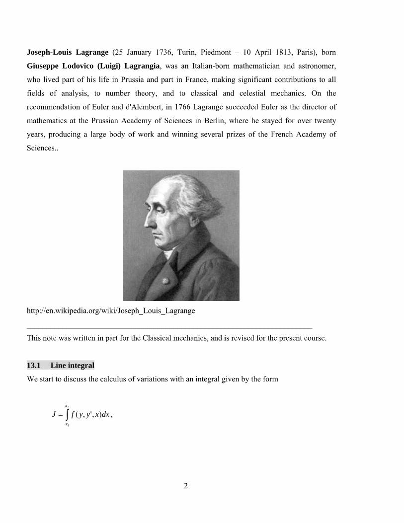
2
Joseph-Louis Lagrange (25 January 1736, Turin, Piedmont – 10 April 1813, Paris), born
Giuseppe Lodovico (Luigi) Lagrangia, was an Italian-born mathematician and astronomer,
who lived part of his life in Prussia and part in France, making significant contributions to all
fields of analysis, to number theory, and to classical and celestial mechanics. On the
recommendation of Euler and d'Alembert, in 1766 Lagrange succeeded Euler as the director of
mathematics at the Prussian Academy of Sciences in Berlin, where he stayed for over twenty
years, producing a large body of work and winning several prizes of the French Academy of
Sciences..
http://en.wikipedia.org/wiki/Joseph_Louis_Lagrange
________________________________________________________________________
This note was written in part for the Classical mechanics, and is revised for the present course.
13.1 Line integral
We start to discuss the calculus of variations with an integral given by the form
2
1
),',(x
x
dxxyyfJ ,

3
where y' = dy/dx. The problem is to find has a stationary function )(xy so as to minimize the
value of the integral J. The minimization process can be accomplished by introducing a
parameter .
x1 x2
y1
y2
y
x
yx
yex
Fig.
11)( yxy , 22 )( yxy ,
)()()( xxyxy
where is a real number and
11)( yxy , 22 )( yxy ,
0)( 1 x , 0)( 2 x
dxdy
y )(0
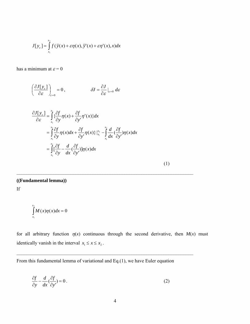
4
2
1
)),(')('),()((][x
x
dxxxxyxxyfyJ
has a minimum at = 0
0][
0
yJ
,
dJ
J 0|
2
1
2
1
2
1
2
1
2
1
)()]'
([
)()'
(|)}('
)(
)}(''
)({][
x
x
x
x
xx
x
x
x
x
dxxy
f
dx
d
y
f
dxxy
f
dx
dx
y
fdxx
y
f
dxxy
fx
y
fyJ
(1)
________________________________________________________________________
((Fundamental lemma))
If
0)()(2
1
x
x
dxxxM
for all arbitrary function (x) continuous through the second derivative, then M(x) must
identically vanish in the interval 21 xxx .
________________________________________________________________________
From this fundamental lemma of variational and Eq.(1), we have Euler equation
0)'
(
y
f
dx
d
y
f. (2)

5
J can have an stationary value only if the Euler equation is valid. The Euler equation clearly
resembles the Lagrange's equation.
In summary,
2
1
)',(x
x
dxxyyfJ .
J = 0 0)'
(
y
f
dx
d
y
f.
13.2 Euler- Lagrange's equations
Now we consider the calculus of variation for the integral
2
1
),',...,',',,...,,( 2121
x
x
nn dxxyyyyyyfJ
We may introduce by setting
)()( 111 xxyy ,
)()( 222 xxyy ,
...............................,
)()( xxyy nnn
where )(1 xy , )(2 xy , ..., are the solutions of the problem,
0)(...)()( 11211 xxx n ,
0)(...)()( 22221 xxx n .
J has a minimum at = 0,

6
0|)(
0
yJ
,
dJ
J 0|
, dy ii ,
2
1
2
1
)]()]'
([
)](''
)([
x
x ii
ii
x
x ii
ii
i
dxxy
f
dx
d
y
f
dxxy
fx
y
fJ
,
at = 0.
2
1
2
1
)()]'
([
)](''
)([
x
x ii
ii
x
x ii
ii
i
dxxy
f
dx
d
y
f
dxxy
fx
y
fJ
Formally, this can be written as
0)]'
([2
1
x
x ii
ii
dxyy
f
dx
d
y
fJ
This is the assertion that J is stationary for the correct path. iy is the virtual displacement. By an
obvious extension of the fundamental lemma, we have
0)'
(
ii y
f
dx
d
y
f,

7
(i = 1, 2, ..., n).
________________________________________________________________________
13.3 Hamilton's principle
William Rowan Hamilton (4 August 1805 – 2 September 1865) was an Irish physicist,
astronomer, and mathematician, who made important contributions to classical mechanics, optics,
and algebra. His studies of mechanical and optical systems led him to discover new
mathematical concepts and techniques. His greatest contribution is perhaps the reformulation of
Newtonian mechanics, now called Hamiltonian mechanics. This work has proven central to the
modern study of classical field theories such as electromagnetism, and to the development of
quantum mechanics.
http://en.wikipedia.org/wiki/William_Rowan_Hamilton
______________________________________________________________________________
Hamilton's principle
Hamilton's principle states that the physical path taken by a particle system moving between
two fixed points in configuration space is one for which the action integral is stationary under a
virtual variation of the path. The action (action integral) is defined as
2
1
2121 ),,...,,,,...,,( dttqqqqqqL nn .

8
The Hamilton's principle is sometimes also called the principle of least action.
The instantaneous configuration of a system is described by the values of the n generated co-
ordinates
),...,,,( 321 nqqqq
and corresponds to a particular point in the configuration space.
t q1,q2,..., qn
t+dt
q1+dq1,q2+dq2,..., qn+dqn
Path of the motion of the system
Fig. Configurational space
The Lagrangian of monogenic system is defined by
VTL
where T is the kinetic energy and V is a potential energy of the system. Here we define the line
integral as
2
1
),,...,,,,...,,( 2121
t
t
nn dttqqqqqqLI .

9
The motion of the system from time t1 to time t2 is such that the line integral has a stationary
value for the actual path of the motion. We can summarize the Hamilton's principle by saying
that the motion is such that the variation of the line integral I for fixed t1 and t2 is zero,
0),...,,,,...,,(2
1
2121 t
t
nn dtqqqqqqLI .
When the system constraints are holonomic, Hamiltonian's principle is both a necessary and
sufficient condition for Lagrange's equation,
0)(
ii q
L
q
L
dt
d
.
Hamilton's principle Lagrange's equation
02
1
t
t
Ldt , 0)(
ii q
L
q
L
dt
d
Then the Euler-Lagrange's equation corresponding to I becomes the Lagrange's equation of
motion.
13.4 Derivation of Lagrange's equation.
We consider the Hamilton's principle with
2
1
),,...,,,,...,,( 2121
t
t
nn dqtqqqqqqLI ,
0),,...,,,,...,,(2
1
2121
t
t
nn dttqqqqqqLdI
I
,
where

10
)()( 111 ttqq ,
)()( 222 ttqq ,
...............................,
)()( ttqq nnn ,
and
)(')( 11 ttqq ,
)(')( 222 ttqq ,
...............................,
)(')( ttqq nnn ,
with
0)(...)()( 11211 ttt n
0)(...)()( 22221 ttt n
q jt1
q jt2
t1
t2
t

11
I has a minimum at = 0.
2
1
2
1
0)()]([
)](')([
t
t ii
ii
t
t ii
ii
i
dttq
L
dt
d
q
L
dttq
Lt
q
LI
at = 0.
0)(
ii q
L
q
L
dt
d
, (i = 1, 2, ..., n).
Here we note that
0
)(
ii
qt ,
ddq
q ii
i
0
dI
I0
or simply
dI
I
Then we have the form of
2
1
0)]([0
t
t ii
ii
dtqq
L
dt
d
q
Ld
II

12
where qi is a virtual displacement.
((Note)) Formulation
Formally we can describe the Hamilton's principle as follows (formulation).
2
1
2
1
2
1
][
),,...,,,,...,,(
),,...,,,,...,,(
2121
2121
t
t i
i
i
i
i
t
t
nn
t
t
nn
dtq
q
Lq
q
Ld
dttqqqqqqLd
dttqqqqqqLI
Here
2
1
2
1
2
1
2
1
2
1
][
t
t i
i
t
t i
itt
i
i
t
t
i
i
t
t
i
i
dtq
L
dt
dq
dtq
L
dt
dq
q
Lq
dtq
dt
d
q
Ldt
q
q
L
with
ii q
qd
, 0)()( 21 tqtq ii .
Then we have
13
2
1
2
1
][
)(
t
t
ii ii
t
t
i
i ii
dtqq
L
dt
d
q
L
dtq
q
L
dt
d
q
LdI
leading to the Lagrange's equation
0
ii q
L
q
L
dt
d
.
13.5 Definition of cyclic
If the Lagrangian of a system does not contain a given co-ordinate qj, then the coordinate is
said to be "cyclic" or "igonorable".
The Lagrange equation of the motion is given by
0
jj q
L
q
L
dt
d
.
The momentum associated with the coordinate qj is defined as
jj q
Lp
.
The terms canonical momentum and conjugate momentum are often also used for pj. using the
expression for pj, the Lagrange's equation can be rewritten as
j
j
q
L
dt
dp
.
For a cyclic coordinate,
14
0
jq
L (qj is not included in L)
0dt
dp j .
This means that
pj = const.
((Conservation theorem))
The generalized momentum conjugate to a cyclic co-ordinate is conserved. If the system is
invariant under the translation along a given direction, the corresponding linear momentum is
conserved. If the system is invariant under the rotation about the given axis, the corresponding
angular momentum is conserved. Thus the momentum conservation theorems are closely
connected with the symmetry properties of the system.
13.6 Example
13.6.1 Free falling

15
y=0 at t = t0
y=y0 at t = 0
yt
At t = 0, the particle is at y = y0. The particle starts to undergo the motion of free falling and
reaches y = 0 at t = t0. The value of y0 is related to t0 by
200 2
1gty .
What is the time dependence of y(t) such that the line integral I over the Lagrangian L takes a
minimum?
)()]([2
1 2 tmgytymL ,

16
0
0
t
LdtI .
((Solution))
We assume that
2)( ctbtaty ,
with
200 2
1)0( gtayy ,
0)( 2000 ctbtaty .
The value of I can be calculated as
)4
3(
6)( 22
30 gcgc
mtcI .
Taking the derivative of I with respect to c, we have a local minimum such that
0)(
c
cI
or
2
gc ,
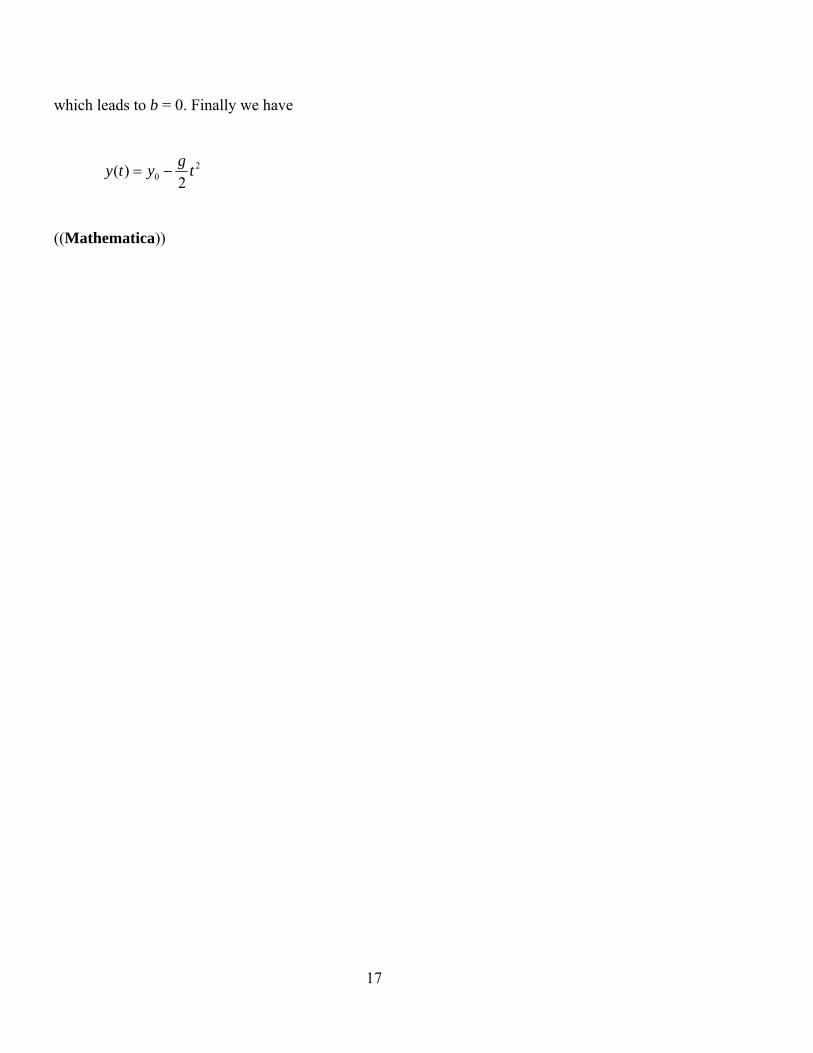
17
which leads to b = 0. Finally we have
20 2
)( tg
yty
((Mathematica))
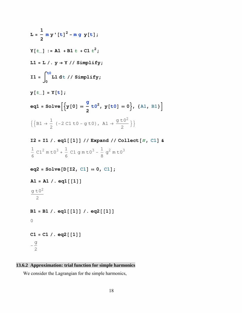
18
L 1
2m y't2 m g yt;
Yt_ : A1 B1 t C1 t2;
L1 L . y Y Simplify;
I1 0
t0L1 t Simplify;
yt_ Yt;
eq1 Solvey0 g
2t02, yt0 0, A1, B1
B1 1
22 C1 t0 g t0, A1
g t02
2
I2 I1 . eq11 Expand Collect, C1 &
1
6C12 m t03
1
6C1 g m t03
1
8g2 m t03
eq2 SolveDI2, C1 0, C1;
A1 A1 . eq11g t02
2
B1 B1 . eq11 . eq210
C1 C1 . eq21
g
2
13.6.2 Approximation: trial function for simple harmonics
We consider the Lagrangian for the simple harmonics,

19
)cos1(2
1 22 mglmlL .
For ≈ 0,
...!4!2
1cos42
)242
(2
1 4222 mglmlL .
The Lagrange's equation is given by
LL
dt
d .
Since
2mlL
. and )6
(3
mglL
,
we have
0)6
(3
2 mglml ,
or
0)6
(3
20
,
where

20
l
g0 .
When
x , 12 ml , 6
20 (>0)
we get
0320 xxx .
4220
2
4)(
2
1xxxL
.
We now consider the integral
2
1
),,(t
t
dttxxLI .
When = 0,
)sin( 00 tAx

21
t
x
O pw
For small (≈ 0), we assume that
)sin( tAx (trial function)
)cos( tAx
Here A and are unknown parameters. We choose
t1 = 0, 2
2 t .
0)( 1 tx , 0)( 2 tx (fixed).
/2
0
2sin tdt ,
/2
0
2cos tdt
4
3sin
/2
0
4 tdt
Using these results, we have
22
420
22
4
3
4)(
2
1AAI
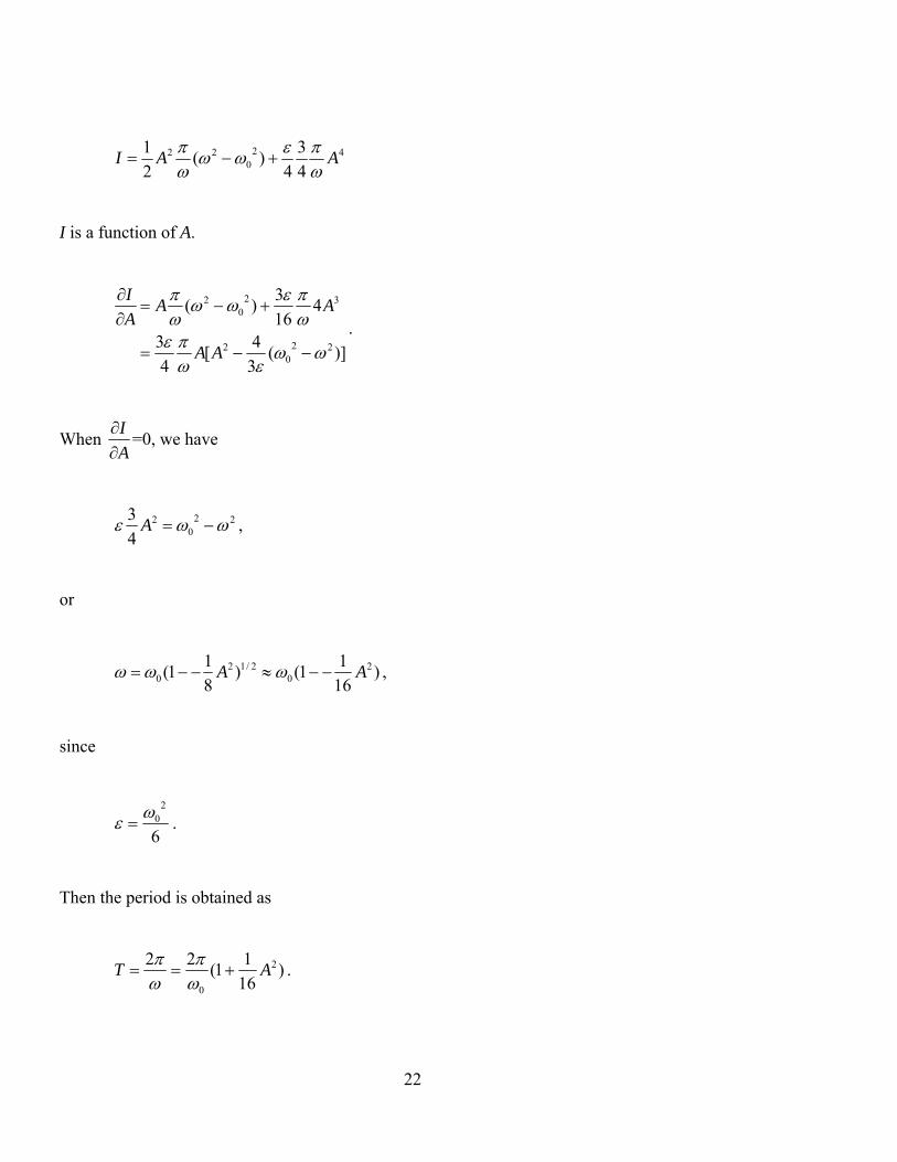
I is a function of A.
)](3
4[
4
3
416
3)(
220
2
320
2
AA
AAA
I
.
When A
I
=0, we have
220
2
4
3 A ,
or
)16
11()
8
11( 2
02/12
0 AA ,
since
6
20 .
Then the period is obtained as
)16
11(
22 2
0
AT
.
23
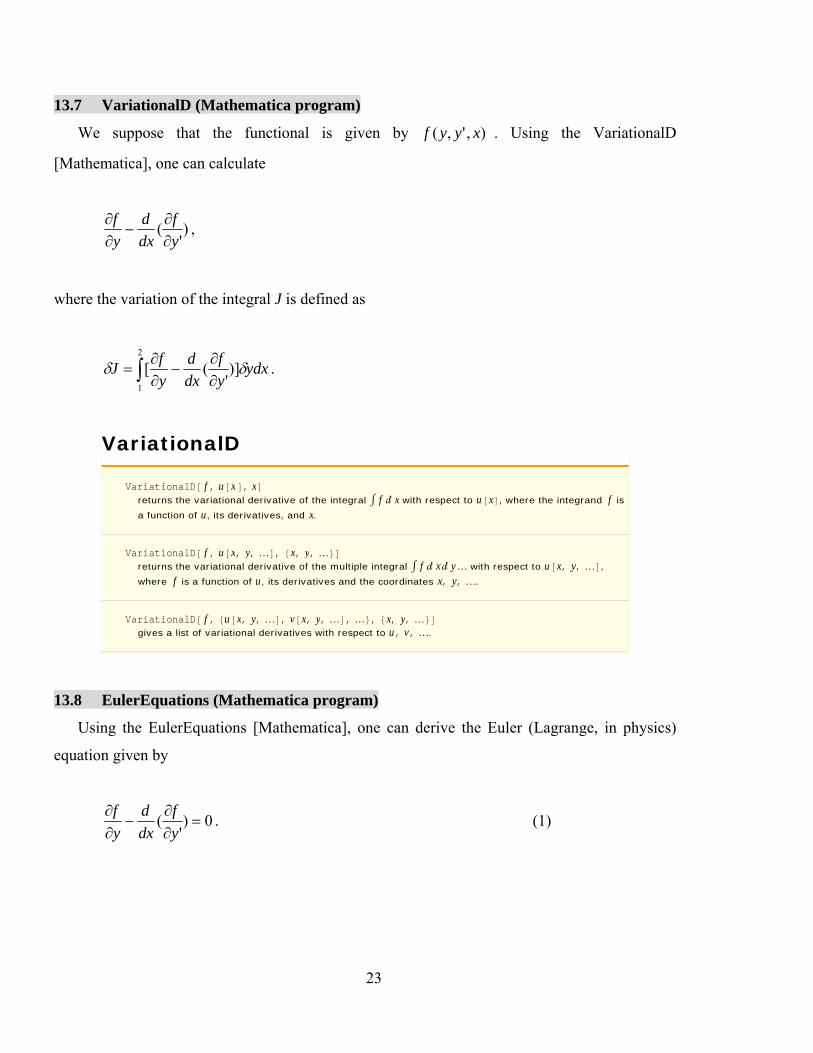
13.7 VariationalD (Mathematica program)
We suppose that the functional is given by ),',( xyyf . Using the VariationalD
[Mathematica], one can calculate
)'
(y
f
dx
d
y
f
,
where the variation of the integral J is defined as
ydxy
f
dx
d
y
fJ ])
'([
2
1
.
VariationalD
VariationalD f , ux, xreturns the variational derivative of the integral f „ x with respect to ux, where the integrand f is a function of u, its derivatives, and x.
VariationalD f , ux, y, …, x, y, … returns the variational derivative of the multiple integral f „ x„ y… with respect to ux, y, …, where f is a function of u, its derivatives and the coordinates x, y, ….
VariationalD f , ux, y, …, vx, y, …, …, x, y, … gives a list of variational derivatives with respect to u, v, ….
13.8 EulerEquations (Mathematica program)
Using the EulerEquations [Mathematica], one can derive the Euler (Lagrange, in physics)
equation given by
0)'
(
y
f
dx
d
y
f. (1)
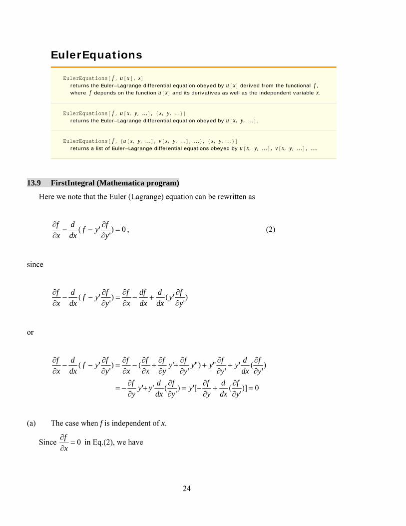
24
EulerEquations
EulerEquations f , ux, xreturns the Euler–Lagrange differential equation obeyed by ux derived from the functional f , where f depends on the function ux and its derivatives as well as the independent variable x.
EulerEquations f , ux, y, …, x, y, … returns the Euler–Lagrange differential equation obeyed by ux, y, ….
EulerEquations f , ux, y, …, vx, y, …, …, x, y, …returns a list of Euler–Lagrange differential equations obeyed by ux, y, …, vx, y, …, ….
13.9 FirstIntegral (Mathematica program)
Here we note that the Euler (Lagrange) equation can be rewritten as
0)'
'(
y
fyf
dx
d
x
f, (2)
since
)'
'()'
'(y
fy
dx
d
dx
df
x
f
y
fyf
dx
d
x
f
or
0)]'
([')'
(''
)'
(''
")"'
'()'
'(
y
f
dx
d
y
fy
y
f
dx
dyy
y
f
y
f
dx
dy
y
fyy
y
fy
y
f
x
f
x
f
y
fyf
dx
d
x
f
(a) The case when f is independent of x.
Since 0
x
f in Eq.(2), we have
25
0)'
'(
y
fyf
dx
d,
or
tconsy
fyf tan
''
. (3)
Thus, when f is independent of x, FirstIntegrals[f, y(x), x] leads to the calculation of '
'y
fyf
.
This corresponds to the Hamiltonian (or energy function) in the physics.
(b) The case when f is independent of y.
Since 0y
f in Eq.(1), we have
tconsy
ftan
'
. (4)
When f is independent of y, FirstIntegrals[f, y(x), x] leads to the calculation of 'y
f
((Note))
When you use FirstIntegrals[f, y(x), x] in your Mathematica program, yo do not have to check
in advance whether f is independent of y or f is independent of x. The Mathematica will check for
you automatically. In this sense, the FirstIntegrals are a very convenient program.

26
FirstIntegrals
FirstIntegrals f , xt, treturns a list of first integrals corresponding to the coordinate xt and independent variable t of the integrand f .
FirstIntegrals f , xt, yt, …, t returns a list of first integrals corresponding to the coordinates x, y, … and independent variable t.
((Mathematica))
Here is an example of the simple harmonics. The Lagrangian is given by
22
2
1
2
1),,( kxxmtxxL
Needs"VariationalMethods`";
L 1
2m x't2
1
2k xt2;
EulerEquationsL, xt, tk xt m xt 0
FirstIntegralsL, xt, tFirstIntegralt
1
2k xt2 m xt2
VariationalDL, xt, tk xt m xt
______________________________________________________________________
13.10 Shortest distance between two points in a plane

27
x1 x2
y1
y2
y
x
Fig. Varied paths of the function of y(x) in the one dimensional extremum problem.
22
22 '11 ydxdx
dydxdydxds
The total length of any curve going between points 1 and 2 is
2
1
2
1
),',(x
x
x
x
xyydxfdsI ,
with
2'1),',( yxyyf .
We calculate the Euler equation
28
0)'
(
y
f
dx
d
y
f
Since
0y
f,
2'1
'
' y
y
y
f
= const.
we have
ay ' (= constant).
or
baxy ,
which is the equation of the straight line. The constants a and b are determined by the condition
that the curve passes through the two end points (x1, y1) and (x2, y2).
In general, curves that give the shortest distance between two points on a given surface are
called the geodesics of the surface.
((Mathematica))

29
Clear"Global`" "VariationalMethods`"
F 1 yx2
1 yx2
eq1 VariationalDF, yx, x
yx1 yx232
eq2 EulerEquationsF, yx, x
yx1 yx232
0
eq3 FirstIntegralsF, yx, xFirstIntegraly
yx1 yx2
, FirstIntegralx 1
1 yx2
eq4 yx
1 yx2
2
c2
yx2
1 yx2 c2
eq5 Solveeq4, y'xyx
c
1 c2, yx
c
1 c2
Since y'[x] is constant, y[x] is a straight line.
13.11 Minimum surface of revolution

30
Suppose we form a surface of revolution by taking some curve passing between two fixed end
points, and revolving it about the y axis. The problem is to find the curve for which the surface
area is a minimum.
222 '1)()( ydxdydxds
The area of a strip of the surface is
dxyxxds 2'122
2
1
),',(x
x
dxxyyfA
with
2'12),',( yxxyyff
Since

31
0y
f,
2'1
'2
' y
yx
y
f
=const
we have
0)'1
'(
2
y
xy
dx
d, a
y
xy
2'1
'
or
22'
ax
a
dx
dyy
Then we get
ba
xha
ax
dxay
)(arccos
22,
or
)cosh(a
byax
,
which is the equation of a catenary.
((Mathematica))
32
Clear"Global`" "VariationalMethods`"
F x 1 y'x2
x 1 yx2
eq1 VariationalDF, yx, xyx yx3 x yx
1 yx232
eq2 EulerEquationsF, yx, xyx yx3 x yx
1 yx232 0
eq3 FirstIntegralsF, yx, xFirstIntegraly
x yx1 yx2
eq4 x yx1 yx2
2
a2
x2 yx2
1 yx2 a2
eq5 Solveeq4, y'xyx
a
a2 x2, yx
a
a2 x2
eq51 eq52 . Rule Equal

33
eq6 eq511yx
a
a2 x2
eq7 DSolveeq6, ya b, yx, x Simplify
yx b a Loga a Logx a2 x2
eq8 Y yx . eq71Y b a Loga a Logx a2 x2
eq9 Solveeq8, x Expand
x 1
2a
baY
a 1
2a
baY
a
eq10 X x . eq91 . a 1, b 2
X 2Y
22Y
2
ContourPlotEvaluateeq10, X, 0, 5, Y, 1, 5, ContourStyle Red, Thick,
Background LightGray
0 1 2 3 4 5
-1
0
1
2
3
4
5
13.12 The brachistochrone problem

34
The brachistochrone problem was one of the earliest problems posed in the calculus of
variations. Newton was challenged to solve the problem in 1696, and did so the very next day. In
fact, the solution, which is a segment of a cycloid, was found by Leibniz, L'Hospital, Newton,
and the two Bernoullis. Johann Bernoulli solved the problem using the analogous one of
considering the path of light refracted by transparent layers of varying density. Actually, Johann
Bernoulli had originally found an incorrect proof that the curve is a cycloid, and challenged his
brother Jacob to find the required curve. When Jacob correctly did so, Johann tried to substitute
the proof for his own.
BRACHIS = SHORT
CHRONOS = TIME
The well-known problem is to find the curve joining two points, along which a particle
falling from rest under the influence of gravity travels from the higher to lower point in the least
time.
x
y
1
2
ds
dxyds 2'1

35
2
1
12 v
dst
If y is measured down from the initial point of release,
02
1 2 mgymv ,
or
gyv 2 .
Then the time t12 is given by
2
1
22
1
2
12
'1
2
1
2
'1dx
y
y
gdx
gy
yt ,
and f(y, y', x) is defined as
y
yxyyf
2'1),',(
.
Euler-Lagrange equation;
y
f
y
f
dx
d
'.
Since

36
)2
1('1 2/32
yyy
f,
)'1(
'
'1
'1
' 22 yy
y
y
y
yy
f
,
we have
2/32
22
2/32
222
2
2
22
2
)]'1([2
'1'"2
)]'1([2
)"2'1')'1("2
)'1(
)'1(2
}"'2)'1('{')'1("
)'1(
'
'
yy
yyyy
yy
yyyyyyy
yy
yy
yyyyyyyyy
yy
y
dx
d
y
f
dx
d
.
Then we get
0
)]'1([2
'1'"2'1
2
12/32
222
2/3
yy
yyyyy
y
0]'1'"2[)'1('11 222/322/32
2/3 yyyyyyyy
0]'1'"2)'1( 2222 yyyyy
0"2)'1( 2 yyy
Thus we find
02
1
'1
"2
yy
y
37
or
0'2
1'
'1
"2
y
yy
y
y
or
constyy ln2
1)'1ln(
2
1 2 .
((Mathematica))
Brachistrochrone prblem
"VariationalMethods`"
F 1 y'x2
yx ;
eq1 VariationalDF, yx, x1 yx2 2 yx yx
2 yx3 1yx2
yx 32
eq2 FirstIntegralsF, yx, x
FirstIntegralx 1
yx 1yx2
yx
eq3 FirstIntegralx . eq21

38
1
yx 1yx2
yx
eq4 eq32 1
2 a Simplify
1
yx yx yx2
1
2 a
eq5 Solveeq4, y'x
yx 2 a yx
yx , yx 2 a yx
yx
eq6 y'x y'x . eq52 0
2 a yx
yx yx 0
eq7 2 a yx
yx yx 0;
This equation can be solved as
dx
dy
y
2 a y
or
x 0
y u
2 a uu

39
eq7 Simplify0
y u
2 a uu, 0 y 2 a, a 0
y 2 a y 2 a 2 a y ArcTan 1
1 2 ay
2 a y
rule1 y 2 a Sin2;
Y y . rule1
2 a Sin2
eq8 FullSimplifyeq7 . rule1, a 0 && 0
2
2 a Cos Sin
X1 eq8 . a 1, 2 Simplify
Sin
Y1 Y . a 1, 22 Sin
22
ParametricPlotX1, Y1, , 0, 6 ,
PlotStyle Hue0, Thickness0.01,
Background GrayLevel0.7,
AspectRatio Automatic, AxesLabel "x", "y"
0 5 10 15x
0.51.01.52.0
y
_______________________________________________________________________
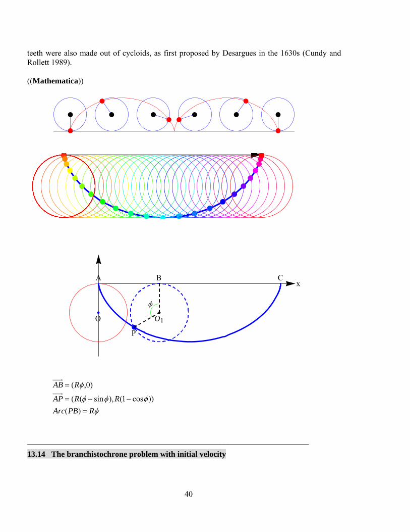
13.13 Cycloid The cycloid is the locus of a point on the rim of a circle of radius rolling along a straight line.
It was studied and named by Galileo in 1599. Galileo attempted to find the area by weighing pieces of metal cut into the shape of the cycloid. Torricelli, Fermat, and Descartes all found the area. The cycloid was also studied by Roberval in 1634, Wren in 1658, Huygens in 1673, and Johann Bernoulli in 1696. Roberval and Wren found the arc length (MacTutor Archive). Gear
40
teeth were also made out of cycloids, as first proposed by Desargues in the 1630s (Cundy and Rollett 1989). ((Mathematica))
xA B C
P
O O1
f
RPBArc
RRAP
RAB
)(
))cos1(),sin((
)0,(
______________________________________________________________________
13.14 The branchistochrone problem with initial velocity

41
When the particle is projected with a kinetic energy 202
1mv , we have
mgzmvmgymv 20
2
2
1
2
1
where
g
vz
2
20
then we have
)(2 zygv
2
1
2
1
22
12
'1
2
1'1
2
1t
t
t
t
dxY
Y
gdx
zy
y
gt
where
zyY
Euler-Lagrange's equation
aYY 2)'1( 2
or
2/1)12
( Y
a
dx
dY

42
For x = 0, Y = z,
)]1(sin[arccos)1[arccos()]1(sin[arccos)1[arccos(
2
a
z
a
za
a
Y
a
Ya
duua
ux
Y
z
)1arccos()1arccos(
a
zy
a
Y
0)1arccos( a
z
a
z1cos 0 ,
a
zy 1cos ,
y = 0, )cos1(2 0
20 ag
vz
)]cos1()cos1[(
)]sin()sin[(
0
00
ay
ax
x
yy
O 2pR
2R
-2Rv0 gR = 0
v0 gR = 2
v0 gR = 2
Fig. Cycloid motion with the initial velocity at y = 0 which is changed as a parameter.

43
)cos1(2 00 gRv , where 0 = 0, /6, /3, /2, 2/3, 5/6, and .
____________________________________________________________
http://www.sewanee.edu/physics/TAAPT/TAAPTTALK.html?x=47&y=53
http://mathworld.wolfram.com/BrachistochroneProblem.html
http://curvebank.calstatela.edu/brach/brach.htm
____________________________________________________________________
13.15 Simple pendulum
We consider a simple harmonics
)cos1(2
1),,(
22
mglmltLL
L is independent of t.
Lagrange equation
0sin l
g ,
with
l
g2
0
First Integral: L is independent of t.
const )cos1(2 20
2
Initial condition: )0()0( v and 0)0(

44
2
)0()cos1(
2
1 22
02 v
)cos1()( 20 U is a potential and
2
)0( 2v is the total energy. When 02)0( v is the critical
angular velocity. For
For 02)0( v , a sinusoidal oscillation is observed.
For 02)0( v , a continuous rotation occurs. In other words, monotonically increases with
increasing t.
See the lecture note on the physics of simple pendulum in much more detail.
http://www2.binghamton.edu/physics/docs/physics-of-simple-pendulum-9-15-08.pdf
((Mathematica))

45
Clear"Global`" "VariationalMethods`"
L 1
2m {2 't2 m g { 1 Cost
g m { 1 Cost 1
2m {2 t2
eq1 VariationalDL, t, tm { g Sint { t
eq2 EulerEquationsL, t, tm { g Sint { t 0
eq3 FirstIntegralsL, t, t Simplify
FirstIntegralt 1
2m { 2 g 1 Cost { t2
eq4 Solveeq2, ''tt
g Sint{
eq5 t t . eq41 0
g Sint{ t 0
eq6 eq5 . g { 02 Simplify
02 Sint t 0

46
phase0_, v0_, 0_, tmax_, opts__ :
Modulenumso1, numgraph,
numso1
NDSolve 02 Sint v't 0, vt 't, 0 0, v0 v0,
t, vt, t, 0, tmax Flatten;
numgraph PlotEvaluatet . numso1, t, 0, tmax, opts,
DisplayFunction Identityphlist
phase0, , 1, 20, PlotStyle Hue5 0.1, AxesLabel "t", "",
Prolog AbsoluteThickness2, Background GrayLevel0.5,
PlotRange All, Ticks Range0, 10, Range3, 3,
DisplayFunction Identity & Range0.1, 2.0, 0.1;
Showphlist, DisplayFunction $DisplayFunction
1 2 3 4 5 6 7 8 9 10t
2
Graphics
phlist
phase0, , 1, 20, PlotStyle Hue2 1.9, AxesLabel "t", "",
Prolog AbsoluteThickness2, Background GrayLevel0.5,
PlotRange All, Ticks Range0, 20, Range0, 8,
DisplayFunction Identity & Range1.9, 2.3, 0.02;
Showphlist, DisplayFunction $DisplayFunction
47
1 2 3 4 5 6 7 8 9 10 11 12 13 14 15 16 17 18 19 20t
2
3
4
5
6
7
8
Graphics
phlist
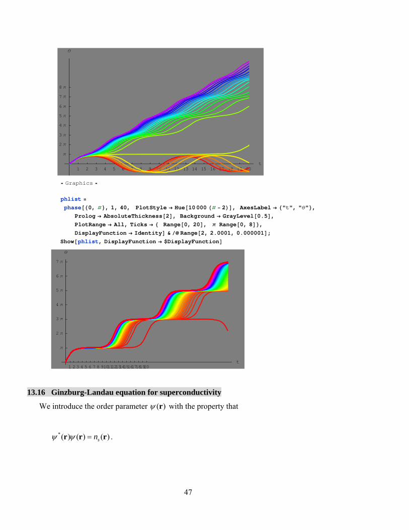
phase0, , 1, 40, PlotStyle Hue10 000 2, AxesLabel "t", "",
Prolog AbsoluteThickness2, Background GrayLevel0.5,
PlotRange All, Ticks Range0, 20, Range0, 8,
DisplayFunction Identity & Range2, 2.0001, 0.000001;
Showphlist, DisplayFunction $DisplayFunction
1 2 3 4 5 6 7 8 91011121314151617181920t
2
3
4
5
6
7
13.16 Ginzburg-Landau equation for superconductivity
We introduce the order parameter )(r with the property that
)()()(* rrr sn .
48
which is the local concentration of superconducting electrons. We first set up a form of the free
energy density Fs(r),
8)(
2
1
2
1)(
22*
*
42 BAr
c
q
imFF Ns
where is positive and the sign of is dependent on temperature. We must minimize the free
energy with respect to the order parameter (r) and the vector potential A(r). We set
drFs )(r
where the integral is extending over the volume of the system. If we vary
)()()( rrr , )()()( rArArA ,
we obtain the variation in the free energy such that
By setting 0 , we obtain the GL equation
02
12*
*
2
A
c
q
im
,
and the current density
AJcm
q
im
qs *
22***
*
*
][2
,
or
49
])()([2
***
**
*
AAJc
q
ic
q
im
qs
At a free surface of the system we must choose the gauge to satisfy the boundary condition that
no current flows out of the superconductor into the vacuum.
0 sJn
((Mathematica))
50
Derivation of Ginzburg Landau equation
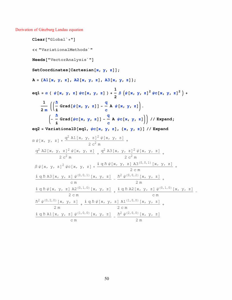
Clear"Global`" "VariationalMethods`"
Needs"VectorAnalysis`"SetCoordinatesCartesianx, y, z;
A A1x, y, z, A2x, y, z, A3x, y, z;
eq1 x, y, z cx, y, z 1
2 x, y, z2 cx, y, z2
1
2 m
—
Gradx, y, z q
cA x, y, z .
—
Gradcx, y, z q
cA cx, y, z Expand;
eq2 VariationalDeq1, cx, y, z, x, y, z Expand
x, y, z q2 A1x, y, z2 x, y, z2 c2 m
q2 A2x, y, z2 x, y, z2 c2 m
q2 A3x, y, z2 x, y, z
2 c2 m
x, y, z2 cx, y, z q — x, y, z A30,0,1x, y, z2 c m
q — A3x, y, z 0,0,1x, y, zc m
—2 0,0,2x, y, z
2 m
q — x, y, z A20,1,0x, y, z2 c m
q — A2x, y, z 0,1,0x, y, z
c m
—2 0,2,0x, y, z2 m
q — x, y, z A11,0,0x, y, z
2 c m
q — A1x, y, z 1,0,0x, y, zc m
—2 2,0,0x, y, z
2 m
51
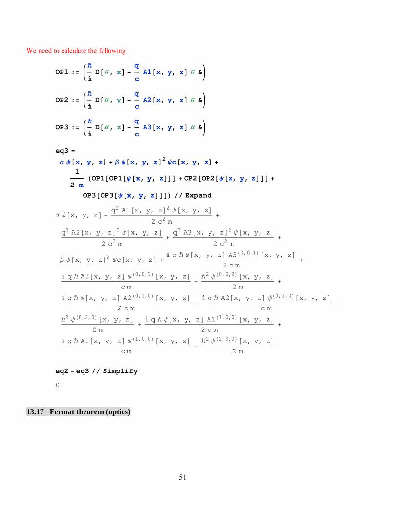
We need to calculate the following
OP1 :—
D, x q
cA1x, y, z &
OP2 :—
D, y q
cA2x, y, z &
OP3 :—
D, z q
cA3x, y, z &
eq3
x, y, z x, y, z2 cx, y, z 1
2 mOP1OP1x, y, z OP2OP2x, y, z
OP3OP3x, y, z Expand
x, y, z q2 A1x, y, z2 x, y, z2 c2 m
q2 A2x, y, z2 x, y, z2 c2 m
q2 A3x, y, z2 x, y, z
2 c2 m
x, y, z2 cx, y, z q — x, y, z A30,0,1x, y, z2 c m
q — A3x, y, z 0,0,1x, y, zc m
—2 0,0,2x, y, z
2 m
q — x, y, z A20,1,0x, y, z2 c m
q — A2x, y, z 0,1,0x, y, z
c m
—2 0,2,0x, y, z2 m
q — x, y, z A11,0,0x, y, z
2 c m
q — A1x, y, z 1,0,0x, y, zc m
—2 2,0,0x, y, z
2 m
eq2 eq3 Simplify
0
13.17 Fermat theorem (optics)
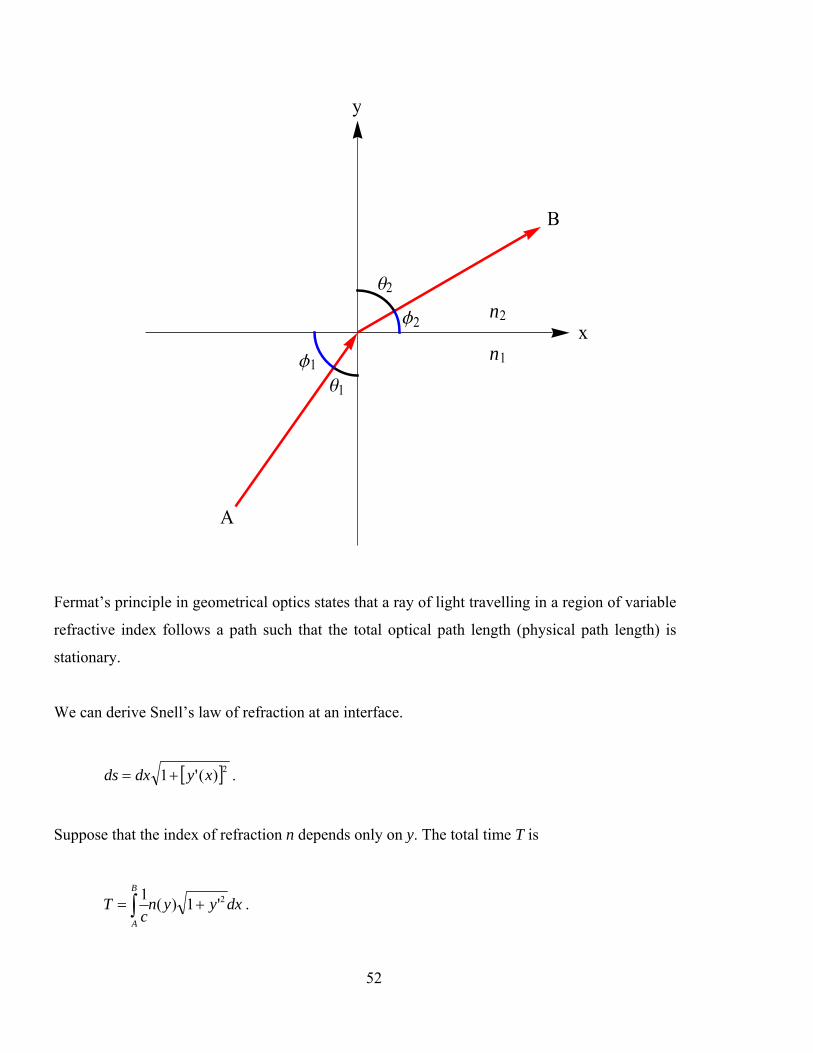
52
x
y
B
A
q2
f2
q1
f1
n2
n1
Fermat’s principle in geometrical optics states that a ray of light travelling in a region of variable
refractive index follows a path such that the total optical path length (physical path length) is
stationary.
We can derive Snell’s law of refraction at an interface.
2)('1 xydxds .
Suppose that the index of refraction n depends only on y. The total time T is
dxyync
TB
A
2'1)(1
.

53
Since the integrand does not contain the independent variable x explicitly, we use the first
integral
2'1)( yynf ,
0'
'
y
fyf ,
or
ky
yny
yynyyyn
22
2
'1
1)(
'1
')(''1)( ,
where k is constant. y’ is the tangent of the angle between the instantaneous direction of the ray
and the x axis.
Since tan'y ,
cos)(tan1
)(
'1
1)(
22ynk
yn
yyn
,
or
2211 coscos nn ,
or
Snell’s law

54
2211
2211
sinsin
)2
cos()2
cos(
nn
nn
.
_____________________________________________________________________+
13.18 Extension of Hamiltonian's principle to nonholonomic systems
It is possible to extend Hamiltonian's principle, at least in a formal sense, to cover certain
types of nonholonomic systems. With nonholonomic systems the generalized co-ordinates are
not independent of each other, and it is not possible to reduce them further by means of Eqs. of
constraint of the form;
0),,...,,( 21 tqqqf n .
It appears that a resonably straightforward treatment of nonholonomic systems by a variational
principle is possible, only when Eqs. of constraint can be put in the form
01
dtadqa lt
n
kklk ,
(l = 1, 2, ..., m.)
a linear relation connecting the differentials of q's. Note that alk and alt may be functions of q's
and t.

55
qk t1
qk t2
qk tdqk
t1
t2
t
t
The constraint Eqs. valid for the virtual displacement are
01
n
kklk qa , (1)
where t = const. We can use Eq.(1) to reduce the number of virtual displacements ti independent
ones.
13.19 Method of Lagrange undetermined multipliers
If Eq.(1) holds, then we have
01
n
kklkl qa . (2)
(l = 1, 2, ....., m).
where l are undetermined quantities;

56
),,...,,( 21 tqqq nll
In addition, we have Hamilton's principle given by
02
1
t
t
Ldt ,
is assumed for the nonholonomic system.
0)(2
1 1
t
t
n
kk
kk
L
dt
d
q
LdtI
(3)
From Eq.(2)
2
1
0,
t
t lkklkl qadt , (4)
The sum of Eq.(3) and (4) then yields the relation
0)(2
1 1 1
t
t
n
kk
m
llkl
kk
qaq
L
dt
d
q
Ldt
The kq 's are still not independent. They are connected by the m relations.
01
n
kklk qa (l = 1, 2, ..., m).
or
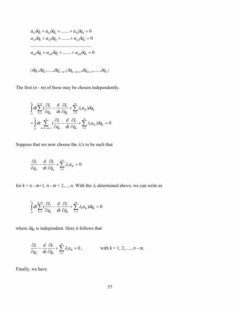
57
0.......
....................................................
0.......
0.......
2211
2222121
1212111
nmnmm
nn
nn
qaqaqa
qaqaqa
qaqaqa
|,.....,,|,,.....,,| 2121 nmmnmn qqqqqq
The first (n - m) of these may be chosen independently.
0)(
)(
2
2
1 1 1
1 1 1
t
t
n
mnkk
m
llkl
kk
t
t
mn
kk
m
llkl
kk
qaq
L
dt
d
q
Ldt
qaq
L
dt
d
q
Ldt
Suppose that we now choose the l's to be such that
01
m
llkl
kk
aq
L
dt
d
q
L
for k = n - m+1, n - m + 2,..., n. With the l determined above, we can write as
0)(2
1 1 1
t
t
mn
kk
m
llkl
kk
qaq
L
dt
d
q
Ldt
where qk is independent. Here it follows that
m
llkl
kk
aq
L
dt
d
q
L
1
0
, with k = 1, 2,....., n - m.
Finally, we have

58
m
llkl
kk
aq
L
dt
d
q
L
1
0
for k = 1, 2, ...., n.
((Note))
We have now (n + m) unknown parameters
(q1, q2, ....., qn),
(1, 2, ...., m),
The additional equations needed are exactly the equations of constraint liking up the qk's
01
lt
n
kklk aqa (l = 1, 2, ..., m)
13.20
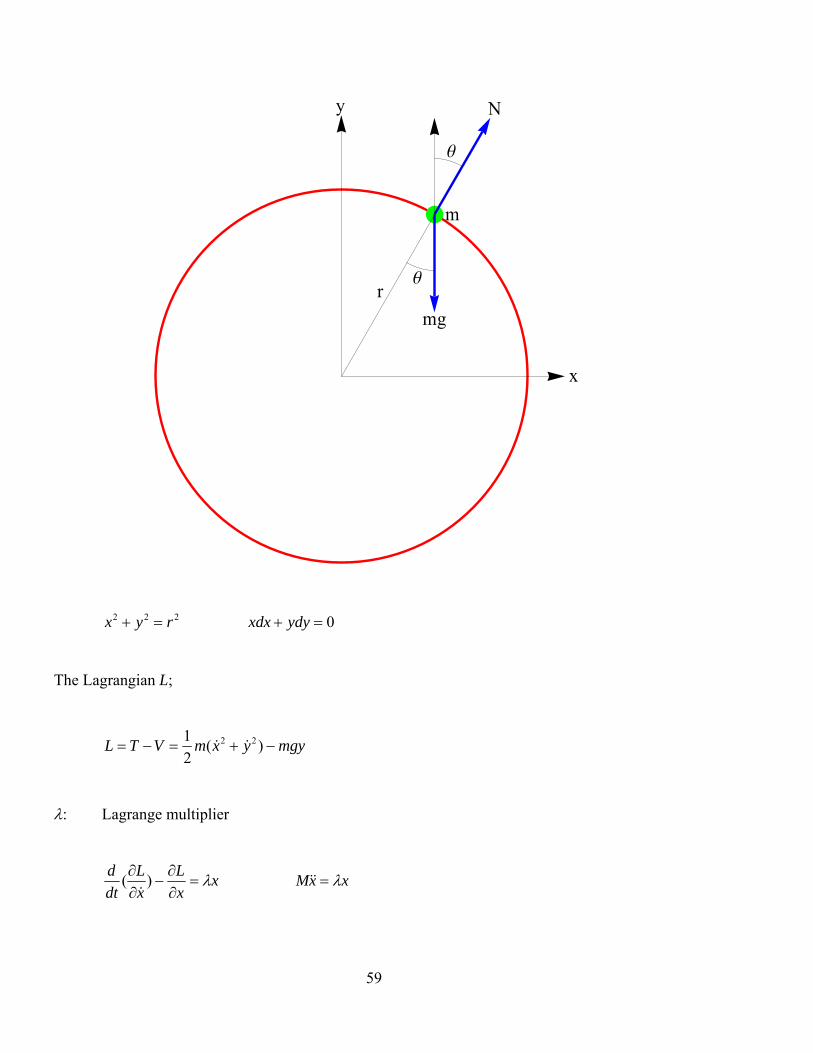
59
x
y N
m
mg
r
q
q
222 ryx 0 ydyxdx
The Lagrangian L;
mgyyxmVTL )(2
1 22
: Lagrange multiplier
xx
L
x
L
dt
d
)(
xxM

60
yy
L
y
L
dt
d
)(
ymgyM
((Note))
ymmgr
yNmgNFy cos
xmr
xNNFx sin
r
N
with
222 ryx 0 yyxx ,
022 yxyyxx
xxr
Nxxm .
ymgyyr
Nyym .
ymgyyxxr
Nyyxxm )()(
or
0])(2
1[ 22 mgyyxm
dt
d

61
mgrmgyyxm )(2
1 22 (energy conservation)
What is the normal force N?
2xr
Nxxm .
mgyyr
Nyym 2 .
or
mgyyxr
Nyyxxm )()( 22
mgyyxr
Nyxm )()( 2222
Since 222 ryx ,
mgyNrmgyyxr
Nyrmg )()(2 22
or
)23( r
ymgN
When N = 0,

62
cos3
2
r
y.
13.21 Example: Rolling of hollow cylinder on the incline
M
r
q
f
O
A x
B
C l
Equation of rolling constraint,
rxOA , or 0 rddx .
Lagrangian L is given by
sin)(2
1
2
1 22 xlMgIxML ,
where I is the moment of inertia and is given by I = Mr2 for the hollow cylinder.
: Lagrange multiplier
63
x
L
x
L
dt
d)(
0sin MgxM
rLL
dt
d
)( 02 rMr
with the equation of constraint
rx .
These equations constitute three equations for three unknown , x, and .
2
singx ,
r
g
2
sin ,
2
sin MgxM . (friction force of constraint)
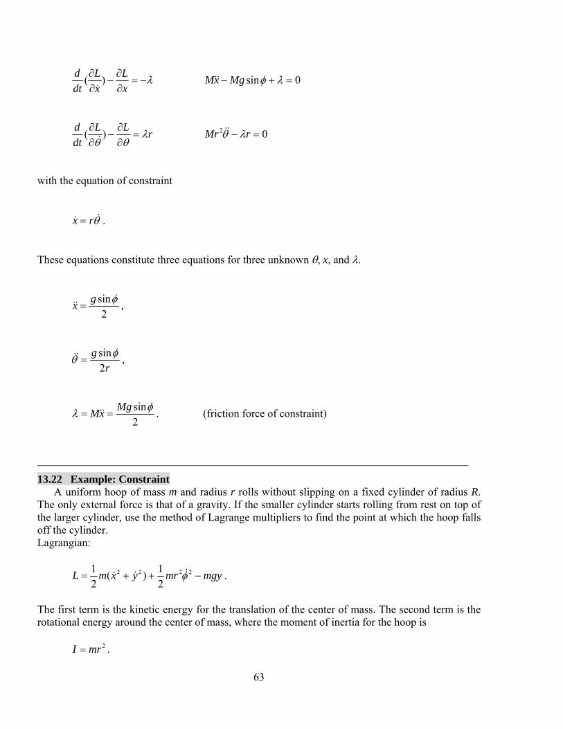
______________________________________________________________________________
13.22 Example: Constraint A uniform hoop of mass m and radius r rolls without slipping on a fixed cylinder of radius R.
The only external force is that of a gravity. If the smaller cylinder starts rolling from rest on top of the larger cylinder, use the method of Lagrange multipliers to find the point at which the hoop falls off the cylinder. Lagrangian:
mgymryxmL 2222
2
1)(
2
1 .
The first term is the kinetic energy for the translation of the center of mass. The second term is the rotational energy around the center of mass, where the moment of inertia for the hoop is
2mrI .

64
Equation of constraint:
222 )( rRyx .
or
0 ydyxdx .
y
xtan ,
or
dy
yx
y
xdyydxd
2
22
22 )(
sec
,
or
drRdyxxdyydx 222 )()( . Then we have
2)( rR
xdyydxd
.
65
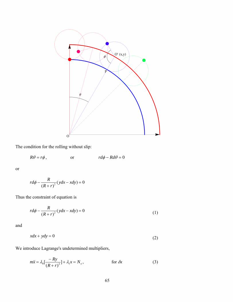
O
q
O' x,y
P
f
The condition for the rolling without slip:
rR , or 0 Rdrd or
0)()( 2
xdyydx
rR
Rrd
Thus the constraint of equation is
0)()( 2
xdyydx
rR
Rrd (1)
and
0 ydyxdx (2)
We introduce Lagrange's undetermined multipliers,
xNxrR
Ryxm
120 ])(
[ , for x (3)
66
yNyrR
Rxmgym
120 ]
)([ , for y (4)
Nrmr 02 , for
where N is the torque of the hoop around its center. Note that
)( xy yNxNrR
rN
.
POOOOP '' , 'OOrR
ROP
'' OOrR
rPO
Then we have
zxy
yyxxyx
zyyxx
yNxNrR
r
NNyxrR
r
NNNPO
e
eeee
eee
)(
)()(
)('
Eq.(3) x + Eq.(4) y + Eq.(5)
0
)(])(
)([ 1120
2
yyxxrR
yxyxRrmrymgyymxxm
or
)(2
1
2
1
2
1 2222 rRmgmrmgyymxm , (6)
or
)(22 2222 rRgrgyyx From Eqs.(1) and (2),
67
)()( 2 yxxy
rR
Rr
,
or
)()(
))(()(
)]2()2[()(
)2()(
)()(
222
2
22224
2
222222224
2
22224
2
24
222
yxrR
R
yxyxrR
R
yyyyxxxxyxyyxxxyrR
R
yxyyxxxyrR
R
yxxyrR
Rr
since
0 yyxx . Thus we get
)()(
222
222 yx
rR
Rr
. (7)
The energy conservation law can be rewritten as
)(22])(
1)[(2
222 rRggy
rR
Ryx
. (9)
At the point where the hoop falls off the cylinder, the component of N along the normal direction is equal to zero.
0)(1
sincos
xNyNrR
NN xyxy ,
or
0 xNyN xy .
Eq.(3) x x + Eq.(4) x y:

68
)(
)()(
)(])(
[])(
[)(
21
221
2212020
yNxN
rRyx
yxrR
Rxy
rR
Rxygyyyxxm
yx
.
We note that
22)(0 yyyxxxyyxxdt
d .
Then we have
21
22 )()()( rRyNxNgyyxm yx . (10)
From Eqs.(9) and (10),
2
222
)(1
)(2
rR
RyrR
gyx
]
)(1
2)(2[
)(
)()(
2
2
22
21
y
rR
RyrR
mg
gyyxm
rRyNxN yx
Then we have
2
2
)(3
)(2
rR
RrR
y
.
from the condition
0 yNxN yx .
_____________________________________________________________________ ((Another method))
A cylinder of radius r and mass m on top of a fixed sphere of radius R. The first sphere is slightly displaced so that it rolls (without slipping) down the second sphere. What is the angle q at which the first sphere loses a contact with the second sphere.
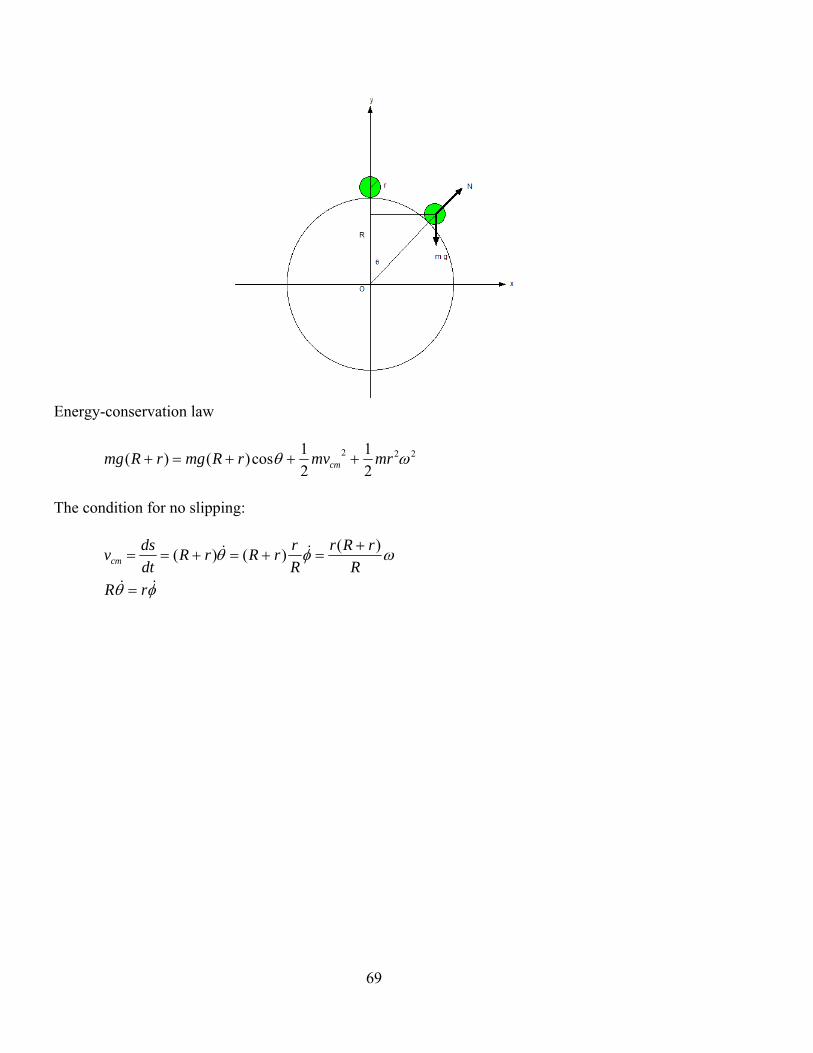
69
Energy-conservation law
222
2
1
2
1cos)()( mrmvrRmgrRmg cm
The condition for no slipping:
rR
R
rRr
R
rrRrR
dt
dsvcm
)()()(

70
where is the rotation angle of the ball
222
2
2
1]1
)([)cos1)(( r
R
rRrRg
(1)
Newton’s second law (centripetal acceleration)
2222
2
222 )(1cos
R
rRmr
R
rRr
rRm
rR
vmNmg cm
When N = 0,
222cos
R
rRrg
(2)
From Eqs.(1) and (2), we have
cos])[(2
1)cos1()( 222 RrRrR
or
2
222
2
)(3
2
22
)(3)(
cos
rR
RRrRrR

71
or
2
2
)(3
)(2cos)(
rR
RrR
rRy
_____________________________________________________________________
13.23 Energy function
Consider a general Lagrangian
),,.....,,,,,.....,,,( 321321 tqqqqqqqqLL nn
t
Lq
q
Lq
q
L
dt
dL
jj
jjj
j
From the Lagrange's equation
jj q
L
q
L
dt
d
)(
.
Then
t
Lq
q
L
dt
d
t
Lq
q
Lq
q
L
dt
d
dt
dL
jj
j
jj
jjj
j
])[(
)(
or
0)(
t
LLq
q
L
dt
d
jj
j
72
We define the energy function given by
j j
j Lq
Lqtqqh
),,(
where
0
t
L
dt
dh.
If the Lagrangian L is not an explicit function of t, then
0dt
dh→ h is conserved
For a conserved system, ),...,( 21 nqqqVV .
jjj q
T
q
Lp
EVTVTT
Lq
Tqtqqh
j jj
)(2
),,(
where E corresponds to the total energy of the system.
13.24 Hamiltonian H
The Hamiltonian is described by
LqptpppqqqHHj
jjnn ),,...,,,,...,,( 2121 ,

73
which then has to be rewritten by eliminating all the generalized velocities in favor of the
generalized momenta
Normally, the Hamiltonian for each problem should be constructed via the Lagrangian
formulation.
(1) Choose a set of generalized co-ordinate qi, and construct
),,...,,,...,,( 2121 tqqqqqL n .
(2) Define the conjugate momenta as a function of tqqqqq n ,,...,,,...,, 2121 .
iniii q
qqLqqqqqpqqpp
),(
),...,,,...,,(),( 2121 .
(3) Use the energy function
),,...,,,...,,((),,...,,,...,,(( 21212121 tqqqqqLqptqqqqqhh ni
iin .
and construct ),,...,,,...,,(( 2121 tqqqqqh n .
(4) Obtain iq as a function of ),,...,,,,...,,( 2121 tpppqqq nn .
(5) Construct ),,...,,,,...,,( 2121 tpppqqqH nn .
Note that The Hamiltonian H is constructed in the same manner as the energy function. But they
are functions of different variables.
____________________________________________________________________
13.25 Hamilton’s equation
dtt
Lqdpdqpdt
t
Lqd
q
Ldq
q
LdL
iiiii
ii
ii
i
)()(

74
where
ii q
Lp
, i
i q
Lp
.
We define the Hamiltonian H as
),,(),,( tqqLqptpqHHi
ii . (Legendre transformation)
dtt
Ldqpdpq
qdpdqpdtt
Lqdpdpq
dLqdpdpqdH
iiiii
iiiii
iiiii
iiiii
)(
)()(
)(
which means that p and q are independent variables.
Consider a function of q, p, and t only. Then we have
dtt
Hdp
p
Hdq
q
HdH
ii
ii
i
)(
which is compared with
dtt
LdqpdpqdH
iiiii
)(
Then we have canonical equations of Hamiltonian
ii p
Hq
, i
i q
Hp
, t
L
t
H

75
13.26 Example
(1) Simple harmonics
22
2
1
2
1kqqmL
qmpq
L
22
22
2
1
2
1
)2
1
2
1(
),,(
kqqm
kqqmqqm
Lqptqqh
Note that
0
t
L
dt
dh. and 0
t
L
or
h = const.
Construction of the Hamiltonian:
m
pq
222
22
2
2
1
22
1
2
1),,( qm
m
pkq
m
pmtpqH
where

76
2mk
(2) Particle (mass m and charge q) in the presence of electromagnetic field
vAv qqmL 2
2
1
Avv
p qmL
or
Apv qm
)2
1()( 2 vAvvAv
vp
qqmqm
LH
or
qqm
qqm
m
qmH
2
22
2
)(2
1
)(1
2
12
1
Ap
Ap
v
13.26 Derivation of Lorentz force from the Lagrangian
The Lagrangian for a particle with charge q in an electromagnetic field described by scalar
potential and vector potential A is

77
vAv qqmL 2
2
1
Find the equation of motion of the charged particle.
)( BvEr qm
where
t
A
E , AB .
((Mathematica))
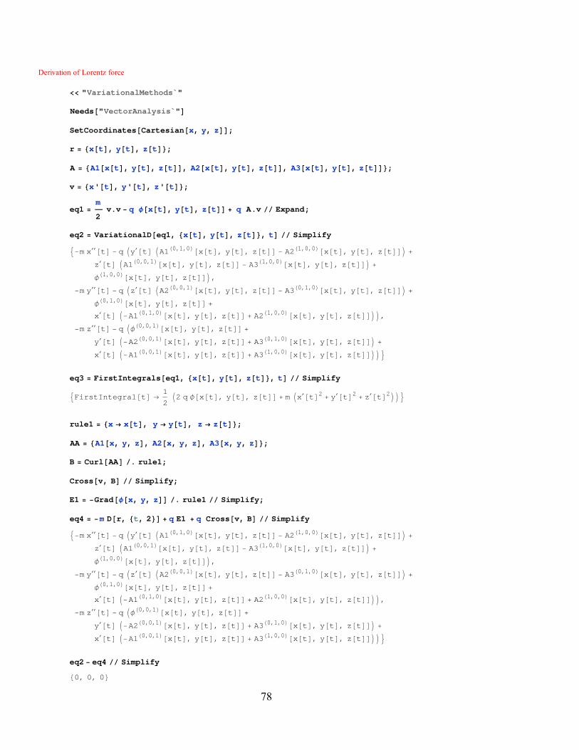
78
Derivation of Lorentz force
"VariationalMethods`"
Needs"VectorAnalysis`"SetCoordinatesCartesianx, y, z;
r xt, yt, zt;
A A1xt, yt, zt, A2xt, yt, zt, A3xt, yt, zt;
v x't, y't, z't;
eq1 m
2v.v q xt, yt, zt q A.v Expand;
eq2 VariationalDeq1, xt, yt, zt, t Simplify
m xt q yt A10,1,0xt, yt, zt A21,0,0xt, yt, zt zt A10,0,1xt, yt, zt A31,0,0xt, yt, zt 1,0,0xt, yt, zt,
m yt q zt A20,0,1xt, yt, zt A30,1,0xt, yt, zt 0,1,0xt, yt, zt xt A10,1,0xt, yt, zt A21,0,0xt, yt, zt,
m zt q 0,0,1xt, yt, zt yt A20,0,1xt, yt, zt A30,1,0xt, yt, zt xt A10,0,1xt, yt, zt A31,0,0xt, yt, zt
eq3 FirstIntegralseq1, xt, yt, zt, t Simplify
FirstIntegralt 1
22 q xt, yt, zt m xt2 yt2 zt2
rule1 x xt, y yt, z zt;
AA A1x, y, z, A2x, y, z, A3x, y, z;
B CurlAA . rule1;
Crossv, B Simplify;
E1 Gradx, y, z . rule1 Simplify;
eq4 m Dr, t, 2 q E1 q Crossv, B Simplify
m xt q yt A10,1,0xt, yt, zt A21,0,0xt, yt, zt zt A10,0,1xt, yt, zt A31,0,0xt, yt, zt 1,0,0xt, yt, zt,
m yt q zt A20,0,1xt, yt, zt A30,1,0xt, yt, zt 0,1,0xt, yt, zt xt A10,1,0xt, yt, zt A21,0,0xt, yt, zt,
m zt q 0,0,1xt, yt, zt yt A20,0,1xt, yt, zt A30,1,0xt, yt, zt xt A10,0,1xt, yt, zt A31,0,0xt, yt, zt
eq2 eq4 Simplify
0, 0, 0
79
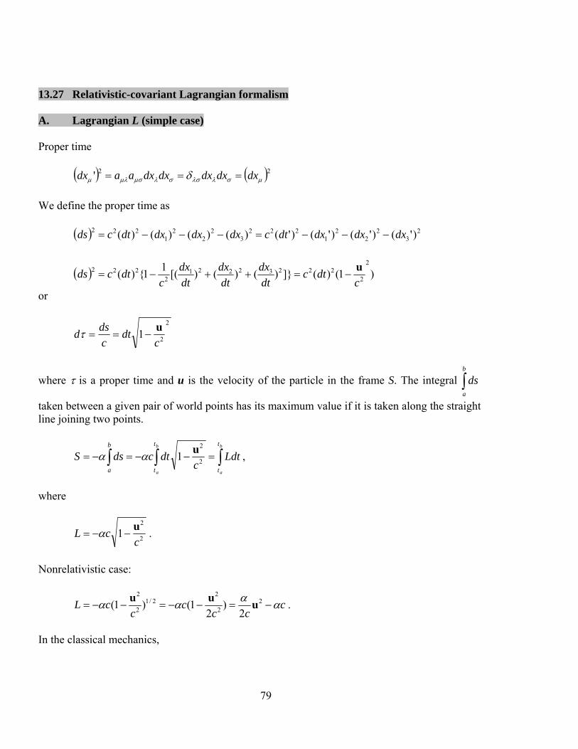
13.27 Relativistic-covariant Lagrangian formalism A. Lagrangian L (simple case) Proper time
22' dxdxdxdxdxaadx
We define the proper time as
23
22
21
2223
22
21
222 )'()'()'()'()()()()( dxdxdxdtcdxdxdxdtcds
)1()(]})()()[(1
1{)(2
222232221
2222
cdtc
dt
dx
dt
dx
dt
dx
cdtcds
u
or
2
21
cdt
c
dsd
u
where is a proper time and u is the velocity of the particle in the frame S. The integral b
a
ds
taken between a given pair of world points has its maximum value if it is taken along the straight line joining two points.
b
a
b
a
t
t
t
t
b
a
Ldtc
dtcdsS 2
2
1u ,
where
2
2
1c
cLu
.
Nonrelativistic case:
ccc
cc
cL 22
22/1
2
2
2)
21()1( u
uu.
In the classical mechanics,

80
22
m
c
or mc .
Therefore the Lagrangian L is given by
2/12
22 )1(
cmcL
u .
The momentum p is defined by
d
dt
dt
dm
d
dmm
c
mL rruu
u
u
up
)(
12
2.
((Note)) This momentum coincides with the components of four-vector momentum p defined by
d
dxmp
d
dxmp
d
dxmp
d
dxmp
44
33
22
11
B. Hamiltonian The Hamiltonian H is defined by
E
c
mcmc
mcmmcmLH
2
2
22
22222
1
)()(
)(
)(
1)(
uu
u
uu
uuuup
,
or
2
2
2
1c
mcE
u
.

81
We have
222
2
2
222
222
2
2
22
2
2
1
)1(
1p
u
uu
u
cm
c
mc
cm
c
cm
c
E.
C. Lagrangian form in the presence of an electromagnetic field The action function for a charge in an electromagnetic field
)( dxqAmcdsSb
a
,
where the second term is invariant under the Lorentz transformation.
)1
,( ciA A , and ),,,( 321 icdtdxdxdxdx .
Then we have
b
a
b
a
dtqc
mcdxqAmcdsS )](1[)(2
22 uA
u.
The integrand in the Lagrangian function of a charge (q) in the electromagnetic field,
)(12
22 uA
uq
cmcL ,
Au
u
up q
c
mL
2
2
1
,
where
)1
,( ciA A .
The Hamiltonian H is given by
82
)1(
12
22
2
2
2
qqc
mce
c
mLH
uAu
uAu
uup ,
or
)1(
12
22
2
2
2
qqc
mce
c
mLH
uAu
uAu
uup ,
q
c
mcH
2
2
2
1u
,
or
222
2
2
222
222
2
)(1
)1(Ap
u
uu
qcm
c
mc
cm
c
qH
.
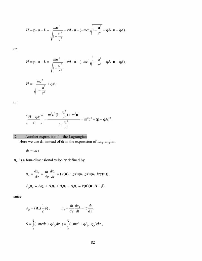
D. Another expression for the Lagrangian
Here we use d instead of dt in the expression of Lagrangian.
cdds
is a four-dimensional velocity defined by
))(,)(,)(,)(( 321 uuuu
icuuu
dt
dx
d
dt
d
dx ,
))((44332211 AuuAAAAA .
since
)1
,( ciA A ,
d
dtic
dt
dx
d
dt 4
4 ,
b
a
b
a
dqAmcdxqAmcdsS )()( 2 ,

83
qAmcL 2 .
E. Lagrangian and Hamiltonian
)(2
)(2 23
22
212
23
22
21 EEE
cBBBFF .
This is invariant under the Lorentz transformation. We may try the Lagrangian density
AJFFL
04
1.
By regarding each component of A as an independent field, we find that
the Lagrange equation
])(
[
x
AL
xA
L
,
is equivalent to
Jx
F0
.
The Hamiltonian density Hem for the free Maxwell field can be evaluated as follows.
FFLem
04
1 ,
)1
(2
1)( 2
22
0
44
0
4
4
4
EBcx
AF
FL
x
A
x
AL
H emem
em
,
or
EBE 02
0
20 2
1
2
1emH ,
drdddHem )2
1(
2
1)()
2
1(
2
1 2
0
200
2
0
20 BErErBEr
.

84
((Note))
0)()(])([)( aErErEErE dddd ,
where E vanishes sufficiently rapidly at infinity.
00
E (in this case).
_________________________________________________________________________