LJMU Research Onlineresearchonline.ljmu.ac.uk/id/eprint/9976/8/stz186.pdf · Numbers of dwarf...

Sedgwick, TM, Baldry, IK, James, PA and Kelvin, LS

The Galaxy Stellar Mass Function and Low Surface Brightness Galaxies from

Core-Collapse Supernovae

http://researchonline.ljmu.ac.uk/9976/

Article

LJMU has developed LJMU Research Online for users to access the research output of the

University more effectively. Copyright © and Moral Rights for the papers on this site are retained by

the individual authors and/or other copyright owners. Users may download and/or print one copy of

any article(s) in LJMU Research Online to facilitate their private study or for non-commercial research.

You may not engage in further distribution of the material or use it for any profit-making activities or

any commercial gain.

The version presented here may differ from the published version or from the version of the record.

Please see the repository URL above for details on accessing the published version and note that

access may require a subscription.

For more information please contact [email protected]

http://researchonline.ljmu.ac.uk/

Citation (please note it is advisable to refer to the publisher’s version if you

intend to cite from this work)

Sedgwick, TM, Baldry, IK, James, PA and Kelvin, LS (2019) The Galaxy

Stellar Mass Function and Low Surface Brightness Galaxies from Core-

Collapse Supernovae. Monthly Notices of the Royal Astronomical Society,

484 (4). pp. 5278-5295. ISSN 0035-8711

LJMU Research Online

http://researchonline.ljmu.ac.uk/

mailto:[email protected]

MNRAS 484, 5278–5295 (2019) doi:10.1093/mnras/stz186Advance Access publication 2019 January 17

The galaxy stellar mass function and low surface brightness galaxies from

core-collapse supernovae

Thomas M. Sedgwick,‹ Ivan K. Baldry , Philip A. James and Lee S. KelvinAstrophysics Research Institute, Liverpool John Moores University, IC2, Liverpool Science Park, 146 Brownlow Hill, Liverpool L3 5RF, UK

Accepted 2019 January 15. Received 2019 January 14; in original form 2018 October 11

ABSTRACT

We introduce a method for producing a galaxy sample unbiased by surface brightness andstellar mass, by selecting star-forming galaxies via the positions of core-collapse supernovae(CCSNe). Whilst matching ∼2400 supernovae from the SDSS-II Supernova Survey totheir host galaxies using IAC Stripe 82 legacy coadded imaging, we find ∼150 previouslyunidentified low surface brightness galaxies (LSBGs). Using a sub-sample of ∼900 CCSNe,we infer CCSN-rate and star formation rate densities as a function of galaxy stellar mass,and the star-forming galaxy stellar mass function. Resultant star-forming galaxy numberdensities are found to increase following a power law down to our low-mass limit of ∼106.4

M⊙ by a single Schechter function with a faint-end slope of α = −1.41. Number densitiesare consistent with those found by the EAGLE simulations invoking a � cold dark mattercosmology. Overcoming surface brightness and stellar mass biases is important for assessmentof the sub-structure problem. In order to estimate galaxy stellar masses, a new code for thecalculation of galaxy photometric redshifts, zMedIC, is also presented, and shown to beparticularly useful for small samples of galaxies.

Key words: methods: statistical – supernovae: general – galaxies: distances and redshifts –galaxies: luminosity function, mass function – galaxies: star formation.

1 IN T RO D U C T I O N

The galaxy stellar mass function (GSMF) is a direct probe of galaxyevolution, as mass is known to be a primary driver of differencesin galaxy evolution. For example, Kauffmann et al. (2003) findgalaxy colours, star formation rates (SFRs), and internal structureall correlate strongly with stellar mass. It is argued by Thomaset al. (2010) that early-type galaxy formation is independent ofenvironment and controlled solely by self-regulation processes,which depend only on intrinsic galaxy properties including mass.Pasquali et al. (2009) demonstrate that star formation and activegalactic nucleus (AGN) activity show the strongest correlations withstellar mass. Past attempts to measure the low-redshift GSMF haveestablished clear evidence of a low-mass upturn in galaxy counts,indicating that low-mass galaxies dominate the galaxy populationby number at current epochs (Baldry et al. 2012, henceforth B12;see also Cole et al. 2001; Bell et al. 2003; Baldry, Glazebrook &Driver 2008; Li & White 2009; Kelvin et al. 2014).

The majority of cosmological simulations today invoke a �

cold dark matter (�CDM) description of our Universe, due to itsability to simultaneously reproduce various observable propertiesof the Universe (Perlmutter et al. 1999; Bennett et al. 2013).

⋆ E-mail: [email protected]

Despite these successes, a major challenge to the �CDM modeltoday is the ‘sub-structure problem’. Numbers of dwarf galaxiesas predicted by straightforward simulations are significantly largerthan those observed, and as a consequence, so too is the overallnumber of galaxies on cosmological scales (Moore et al. 1999).This discrepancy in dwarf galaxy counts is reflected in the form ofthe GSMF.

The observed number density of dwarf galaxies increases down to∼108 M⊙, below which the form of the GSMF is uncertain (B12).Cosmological simulations of galaxy evolution such as EAGLE(Schaye et al. 2015; Crain et al. 2015) and ILLUSTRIS (Genelet al. 2014) are now sophisticated enough to attempt to assess theGSMF into the dwarf regime. In contrast to observational results,the GSMF from these simulations sees number densities continueto increase in the dwarf mass regime, approximately following apower law.

This discrepancy may not be a fault of a �CDM descriptionof our Universe, however, almost all galaxy surveys suffer from acombination of magnitude and surface brightness constraints (Cross& Driver 2002; Wright et al. 2017). Most dwarf systems (typically�108 M⊙; Kirby et al. 2013) have intrinsically lower surfacebrightnesses than their higher mass counterparts, and consequently,the lower mass end of the GSMF may be underestimated dueto sample incompleteness, with lower surface brightness galax-ies more likely to be missed by galaxy surveys. The current

C© 2019 The Author(s)Published by Oxford University Press on behalf of the Royal Astronomical Society

Dow

nlo

aded fro

m h

ttps://a

cadem

ic.o

up.c

om

/mnra

s/a

rticle

-abstra

ct/4

84/4

/5278/5

290332 b

y L

iverp

ool J

ohn M

oore

s U

niv

ers

ity u

ser o

n 1

1 M

arc

h 2

019

http://orcid.org/0000-0003-0719-9385

http://orcid.org/0000-0001-9395-4759

mailto:[email protected]

The GSMF and LSBGs from CCSNe 5279

observed number densities of low-mass galaxies can be treated asa lower limit when constraining evolutionary models (Baldry et al.2008).

Knowing the precise form of the GSMF is clearly crucial shouldwe wish to use it as a diagnostic of galaxy evolution. Developingtechniques to increase completeness of the low-mass end of theGSMF must be the focus should one wish to use it to assess thenature of the physics which controls this evolution.

Here, we develop and implement one such technique, using theStripe 82 Supernova Survey (Sako et al. 2018, henceforth, S18)to produce a sample of galaxies located at the positions of core-collapse supernovae (CCSNe). As CCSNe peak at luminosities of108–109 L⊙, they can be used as pointers to their host galaxies,which may have been missed from previous galaxy surveys dueto their low surface brightness: The Palomar Transient Factory(Law et al. 2009) located low surface brightness galaxies (LSBGs)when combining SN positions with imaging taken pre-supernovaor long after SN peak epoch (Perley et al. 2016). As well as aidingthe identification of LSBGs, a galaxy selection using a completesample of supernovae may significantly reduce surface brightnessand magnitude biases if the host galaxy is identified for each SN ina sample.

Given that the progenitor stars of core-collapse supernovae(CCSNe henceforth) have high masses, it is natural to use themas a tracer of recent star formation. The lower mass limit for zero-age main-sequence stars that end their lives as CCSNe has beenclosely constrained by numerous studies, with the review of Smartt(2009) presenting a consensus value of 8 ± 1 M⊙. The upper masslimit is much more uncertain, due to the possibility that the highestmass stars may collapse directly to black holes, with no visibleexplosion. However, it seems likely that stars at least as massiveas 30 M⊙ explode as luminous CCSNe; Botticella et al. (2017)adopt an upper mass limit of 40 M⊙. The corresponding range oflifetimes of CCSN progenitors is then something like 6–40 Myr,for single star progenitors (see e.g. Maund 2017); mass-exchangein high-mass binary stars can extend these lifetimes (e.g. Smith &Tombleson 2015). Even with this extension, it is clear that on thetime-scales relevant for studies of galaxy evolution, rates of CCSNecan be taken as a direct and virtually instantaneous tracer of thecurrent rate of star formation.

Several studies have made use of CCSNe as an indicator of starformation in the local Universe. On the most local scales, bothBotticella et al. (2012) and Xiao & Eldridge (2015) have comparedCCSN rates and integrated SFRs within a spherical volume of radius11 Mpc centred on the Milky Way, finding good agreement betweenobserved and predicted numbers of SNe. A similar conclusion wasalso reached by Cappellaro, Evans & Turatto (1999), looking ata rather more extended (mean distance ∼40 Mpc) sample of SNeand host galaxies. Other studies have used CCSNe to probe starformation at intermediate redshifts, e.g. Dahlen et al. (2004), whoinvestigated the increase in the cosmic SFR out to redshift ∼0.7, andBotticella et al. (2017) whose sample of 50 SNe mainly occurred inhost galaxies in the redshift range 0.3–1.0. Pushing to still higherredshifts, Strolger et al. (2015) have investigated the cosmic SFhistory out to z ∼ 2.5 using CCSNe within galaxies from theCANDELS (Grogin et al. 2011) and CLASH (Postman et al. 2012)surveys.

Supernovae have also been used to investigate SF in differentenvironments and types of galaxies, e.g. in starbursts (Miluzio et al.2013) and galaxies with AGNs (Wang, Deng & Wei 2010), andto determine the metallicity dependence of the local SF rate (Stollet al. 2013).

By selecting galaxies using CCSNe and measuring galaxy stellarmasses, the resultant number densities as a function of mass implyCCSN-rate densities as a function of mass (ρCCSN) in units ofyr−1 Mpc−3, under the assumption that the CCSN sample itself iscomplete. By assuming a relationship between CCSN rate and SFR,we are able to trace star formation rate densities (SFRDs) (M⊙yr−1

Mpc−3). The well-established star-forming galaxy main sequence(Noeske et al. 2007; Davies et al. 2016; McGaugh, Schombert &Lelli 2017; Pearson et al. 2018) can then be used to determinetypical star formation levels expected for a given stellar mass, toinfer star-forming galaxy number densities (Mpc−3) as a functionof galaxy stellar mass (the GSMF), such that ρCCSN → ρSFR →GSMF.

A programme similar to this work was proposed by Conroy &Bullock (2015), who suggested that SNe detected by the LargeSynoptic Survey Telescope from 2021 could be used as a statisticalprobe of the numbers and stellar masses of dwarf galaxies. Thiswork can be seen as a precursor to such a study.

The structure of this work is as follows. Section 2 outlines infurther detail the connections between CCSN-rate density, SFRD,and the GSMF, along with the assumptions required to form them.In Section 3, we present the data sets used. In Section 4, we outlineour methodology for drawing from these complete SN and galaxysamples, unbiased by magnitude and surface brightness, as well asour procedure for obtaining photometric redshift estimates. Sec-tion 5 presents resultant SFRD and star-forming GSMF estimatesobtained via a CCSN host galaxy selection, where comparison isdrawn with existing SFRD and GSMF results, both observationaland simulated.

2 C ONVERTI NG CCSN-RATE DENSI TY TO

T H E STA R - F O R M I N G G A L A X Y S T E L L A R

MASS FUNCTI ON

In this section, we represent mathematically the CCSN-rate density,the SFRD, and the GSMF. This is in order to define the connectionsbetween them, and hence, how we are able to arrive at an estimatefor the GSMF by measuring the CCSN-rate density as a function ofhost galaxy stellar mass (M).

For a volume-limited sample of galaxies, the binned GSMF isdefined by

�(M) =1

� logM

N (M)

V(1)

over a mass bin of width � logM, where N is the number of galaxiesin the bin, and V is the volume. In other words, the GSMF is thenumber of galaxies, per unit volume, per logarithmic bin of galaxystellar mass.

The SFRD is often estimated for the entire galaxy population,particularly as a function of redshift (Madau & Dickinson 2014),but it can also be determined as a function of galaxy mass (Gilbanket al. 2010). This can then be given by

ρSFR(M) =1

� logM

∑N

i=1 Si Mi

V, (2)

where Si is the specific star formation rate (SSFR) for each of theN galaxies in a bin. In other words, the SFRD is the summed SFR,per unit volume, per logarithmic bin of stellar mass.

We can approximate the SFRD by considering that the majority ofstar formation in the Universe occurs on the galaxy main sequence(Noeske et al. 2007; Davies et al. 2016; McGaugh et al. 2017). Thissequence represents the relation, and its scatter, of SFR versus mass

MNRAS 484, 5278–5295 (2019)

Dow

nlo

aded fro

m h

ttps://a

cadem

ic.o

up.c

om

/mnra

s/a

rticle

-abstra

ct/4

84/4

/5278/5

290332 b

y L

iverp

ool J

ohn M

oore

s U

niv

ers

ity u

ser o

n 1

1 M

arc

h 2

019

5280 T. M. Sedgwick et al.

for typical star-forming galaxies. The SFRD can then be given by

ρSFR(M) =1

� logM

S(M) M NSF(M)

V(3)

where NSF is number of star-forming galaxies in the bin, M is themid-point mass (assuming � logM ≪ 1), and S is the mean SSFRfor star-forming galaxies.

By star-forming galaxy, we mean all galaxies that are not perma-nently quenched or virtually quenched with minimal residual starformation. In other words, these are the galaxies that are representedby the cosmological SFRD as a function of mass. Note that in theestimate of the mean S, we should include galaxies that are in aquiescent phase but are otherwise representative of the typical star-forming population, and our CCSN host galaxy selection methodnaturally leads to an appropriate contribution from such galaxies.This is relevant for low-mass galaxies that undergo more variationin their SFR with time (see e.g. Skillman 2005; Stinson et al. 2007).The mean S should represent an average over duty cycles in thisregime.

Comparing with equation (1), we note that the SFRD can thenbe rewritten in terms of the GSMF of star-forming galaxies �SF asfollows:

ρSFR(M) = S(M) M �SF(M). (4)

By using a parametrization of SSFR with galaxy stellar mass (e.g.Noeske et al. 2007; Speagle et al. 2014), it is possible to estimatethe GSMF for star-forming galaxies from the SFRD or vice versa.

Next we consider the observed CCSN-rate density. Here wedefine this as the rate of CCSNe observed over a defined volumeof space (redshift and solid angle limited), per unit volume,per logarithmic bin of galaxy stellar mass. From a non-targetedSupernova Survey, like that of Sloan Digital Sky Survey (SDSS;Frieman et al. 2008, S18), this is given by

ρCCSN,obs(M) =1

� logM

nCCSN,obs(M)

τ V, (5)

where nCCSN,obs is the number of observed CCSNe associated withgalaxies in the bin, and τ is the effective rest-frame time over whichCCSNe could be identified. The time period of the supernova survey,in the average frame of the host galaxies (τ ), is shorter than that inthe observed frame (t), such that τ = t/(1+z).

The relationship between the CCSN rate and SFRD is then givenby

ρCCSN,obs(M) = ρSFR(M) ǫ(M) R(M), (6)

where R is the mean ratio of CCSN rate to SFR, which is equivalentto the number of CCSNe per mass of stars formed; and ǫ is the meanefficiency of detecting supernovae. For an apparent-magnitude-limited supernova survey, the latter function accounts for varyingbrightnesses and types of supernova occurring in star-forminggalaxies of a given stellar mass, and the variation in extinctionalong different lines of sight to the supernovae.

By combining these relations we arrive at

�SF =ρCCSN,obs

ǫ R SM, (7)

which explicitly relates CCSN-rate density to the star-formingGSMF. The connection is given in terms of three functions ofgalaxy stellar mass: S is the SSFR relation of the galaxy mainsequence; R is the number of CCSNe per unit mass of stars formed;and ǫ is the efficiency of detecting CCSNe, which depends ontheir luminosity function, and also non-intrinsic effects of sample

selection and survey strategy, in particular, the limiting CCSNdetection magnitude. The basic premise is that these should bea weak function of galaxy stellar mass. We investigate the effectsof varying ε on estimated CCSN-rate densities in Section 5.2, andof varying S on the GSMF in Section 5.4.

3 DATA

This study makes use of three data sets, all of which are data productsof the SDSS. SDSS is a large-area imaging survey of mainly theNorth Galactic cap, with spectroscopy of ∼106 galaxies and stars,and ∼105 quasars (York et al. 2000). The survey uses a dedicated,wide-field, 2.5 m telescope (Gunn et al. 2006) at Apache PointObservatory, New Mexico. A 142 megapixel camera, using a drift-scan mode (Gunn et al. 2006), gathers data in five optical Sloanbroad-band filters, ugriz, approximately spanning the range from3000 to 10 000 Å, on nights of good seeing. Images are processedusing the software of Lupton et al. (2001) and Stoughton et al.(2002). Astrometric calibrations are achieved by Pier et al. (2003).Photometric calibrations are achieved using methods described byHogg et al. (2001) and Tucker et al. (2006) via observations ofprimary standard stars observed on a neighbouring 0.5 m telescope(Smith et al. 2002).

We make use of data associated with the Stripe 82 region, a 275deg2 equatorial region of sky (Baldry et al. 2005). The region spansroughly 20h < RA < 4h and –1.26◦ < Dec. < 1.26◦. Between1998 and 2004, the region was scanned ∼80 times. A further ∼200images were taken between 2005 and 2007, as part of the SDSS-IISupernova Survey (Frieman et al. 2008, S18).

The SDSS-II Supernova Survey data release outlined in S18forms the basis of the supernova sample used for this study. 10 258transient sources were identified using repeat ugriz imaging of theregion, with light curves and follow-up spectra used for transientclassifications, all of which are utilized in this study to produce anSN sample, with great care taken to ensure its completeness and theremoval of non-SN transients.

We aim to produce a galaxy sample selected via the SNe whichthey host. Host galaxies for many of the transient sources werealready identified as part of the Supernova Survey. However, in thisstudy we revisit host galaxy identification for two reasons: (i) Thereis now access to deeper, coadded SDSS imaging with which tosearch for the host galaxy. (ii) There is often a natural bias towardsassigning a transient to a higher surface brightness galaxy when oneor more lower surface brightness galaxy is nearby. Our method oftransient-galaxy matching is designed specifically to address thisbias.

To form this galaxy sample, we make use of both single-epochimaging and multiple epoch SDSS imaging. Single-epoch imagingpublished as part of SDSS-IV DR14 forms our initial galaxy sample(referred in this study as the SDSS sample for simplicity), and thesample of stars used for the removal of variable stars from our SNsample, as outlined in Sections 4.1.1 and 4.2.1, respectively. Galaxyand star classification is described in section 4.4.6 of Stoughton et al.(2002).

We then turn to coadds of multiple epoch imaging. The IACStripe 82 legacy project (Fliri & Trujillo 2016) performs medianstacking of existing legacy Stripe 82 data, with additional complexsky-subtraction routines applied thereafter, in order to reach theextremely faint limits of the data (∼28.5 mag arcsec2 to 3σ for10 × 10 arcsec2). The IAC Stripe 82 legacy catalogue hence forms adeeper sample of objects used for this investigation. Approximately100 single-epoch images are median stacked per SN region, to

MNRAS 484, 5278–5295 (2019)

Dow

nlo

aded fro

m h

ttps://a

cadem

ic.o

up.c

om

/mnra

s/a

rticle

-abstra

ct/4

84/4

/5278/5

290332 b

y L

iverp

ool J

ohn M

oore

s U

niv

ers

ity u

ser o

n 1

1 M

arc

h 2

019


produce the deeper imaging crucial for LSBG detection. Fromthis coadded imaging we aim to identify additional LSBGs notfound by the SDSS sample. IAC Stripe 82 image mosaicking andpostage stamp creation about the positions of our SNe, crucial forhost galaxy identifications, were completed using the Cutout andMosaicking Tool, part of the ARI Survey Imaging Tools, createdby one of the authors (LSK). We compare the completeness ofthe SDSS sample with the sample found by Fliri & Trujillo (2016)from this coadded data, as well with a SEXTRACTOR implementationdesigned as a bespoke search for CCSN host galaxies, using thesame data (Section 4.2.3), in order to demonstrate the sensitivity ofresults to sample incompleteness.

We also require redshift estimates for our SN-galaxy pairs.Approximately 480 of the SN candidates have spectra of their own,from 10 sources outlined in Frieman et al. (2008). We also use hostgalaxy spectra for our SN-galaxy pairs once the host galaxy has beenconfidently identified. The galaxy spectra utilized stem from threemain sources within SDSS. These are the SDSS-II Legacy (Yorket al. 2000), SDSS-II Southern (Baldry et al. 2005), and SDSS-IIIBOSS/SDSS-IV eBOSS surveys (Dawson et al. 2013, 2016). Thelatter contains spectroscopy for galaxies identified as the hosts of3743 of the 10 258 SN candidates in S18, approximately a thirdof which were identified as non-supernovae as a result. Supernovaredshifts are used in cases where both are available. Photometricredshifts of galaxies are calculated from the coadded photometry incases where no spectroscopic redshift is available for an SN-galaxypair, as outlined in Section 4.3.2.

4 M E T H O D O L O G Y

4.1 Selection of the supernova sample

4.1.1 Star removal

In order to produce a sample of CCSNe, we first focus onremoving non-supernovae from the SDSS-II Supernova Surveysample. 10 258 transient sources were found by S18. We buildon their classification attempts by first removing those transientsources categorized as variable stars (objects detected over multipleobserving seasons) and AGNs (identified spectroscopically via theirbroad hydrogen lines).

The main SN classifications of S18 are Type II, Type Ib/c,and Type Ia SNe. We ultimately wish to remove Type Ia SNeto obtain a CCSN sample in order to trace SFRs. However, wekeep likely Type Ia SNe in the sample at this stage to search forLSBGs and to increase the size of our training sample used forthe estimations of galaxy redshifts, as described in Section 4.3.2.At this stage, the sample consists of 6127 transients. Of theseobjects, 1809 are spectroscopically confirmed SNe and a further2305 are, photometrically, deemed very likely to be supernovae,via a combination of Bayesian, nearest-neighbour and light-curvefit probabilities (see S18 for a full description). Those remainingare classified as ‘Unknown’. However, these objects may still besupernovae. For several of these objects it may simply be unclearfrom the photometry what type of supernova is being seen. Forinstance, if probabilities derived from the three aforementionedtechniques give a reasonable likelihood for more than one of TypeIa, Ib/c, or II, the object will be classified as ‘Unknown’.

We match transient positions with all objects of the SDSS-IVDR14 PhotoPrimary catalogue located in the Stripe 82 region withGalactic extinction-corrected r-band magnitude < 22.0 (Petrosian,psf or model) (∼107 objects). We refer to this as the SDSS catalogue

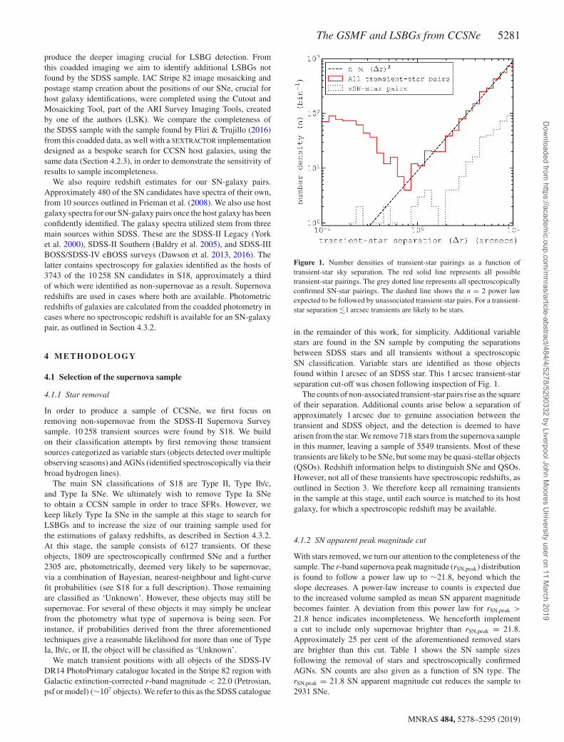
Figure 1. Number densities of transient-star pairings as a function oftransient-star sky separation. The red solid line represents all possibletransient-star pairings. The grey dotted line represents all spectroscopicallyconfirmed SN-star pairings. The dashed line shows the n = 2 power lawexpected to be followed by unassociated transient-star pairs. For a transient-star separation �1 arcsec transients are likely to be stars.

in the remainder of this work, for simplicity. Additional variablestars are found in the SN sample by computing the separationsbetween SDSS stars and all transients without a spectroscopicSN classification. Variable stars are identified as those objectsfound within 1 arcsec of an SDSS star. This 1 arcsec transient-starseparation cut-off was chosen following inspection of Fig. 1.

The counts of non-associated transient-star pairs rise as the squareof their separation. Additional counts arise below a separation ofapproximately 1 arcsec due to genuine association between thetransient and SDSS object, and the detection is deemed to havearisen from the star. We remove 718 stars from the supernova samplein this manner, leaving a sample of 5549 transients. Most of thesetransients are likely to be SNe, but some may be quasi-stellar objects(QSOs). Redshift information helps to distinguish SNe and QSOs.However, not all of these transients have spectroscopic redshifts, asoutlined in Section 3. We therefore keep all remaining transientsin the sample at this stage, until each source is matched to its hostgalaxy, for which a spectroscopic redshift may be available.

4.1.2 SN apparent peak magnitude cut

With stars removed, we turn our attention to the completeness of thesample. The r-band supernova peak magnitude (rSN,peak) distributionis found to follow a power law up to ∼21.8, beyond which theslope decreases. A power-law increase to counts is expected dueto the increased volume sampled as mean SN apparent magnitudebecomes fainter. A deviation from this power law for rSN,peak >

21.8 hence indicates incompleteness. We henceforth implementa cut to include only supernovae brighter than rSN,peak = 21.8.Approximately 25 per cent of the aforementioned removed starsare brighter than this cut. Table 1 shows the SN sample sizesfollowing the removal of stars and spectroscopically confirmedAGNs. SN counts are also given as a function of SN type. TherSN,peak = 21.8 SN apparent magnitude cut reduces the sample to2931 SNe.

MNRAS 484, 5278–5295 (2019)

Dow

nlo

aded fro

m h

ttps://a

cadem

ic.o

up.c

om

/mnra

s/a

rticle

-abstra

ct/4

84/4

/5278/5

290332 b

y L

iverp

ool J

ohn M

oore

s U

niv

ers

ity u

ser o

n 1

1 M

arc

h 2

019


Table 1. Transient counts as a function of type, built from the SDSS-II Supernova Survey sample of 10 258 transients. Counts aredivided into (i) those rejected by a magnitude cut, rSN,peak > 21.8, because of sample incompleteness for fainter transients; (ii) thosebrighter than rSN,peak < 21.8 but rejected as variable stars or AGNs; and (iii) those that are selected for our sample. Variable star countsare shown as the summation of those classified by Sako et al. (2018), by host matching to single-epoch SDSS imaging, and to Stripe82 legacy coadded imaging. AGN counts are shown as the summation of those classified by Sako et al. (2018), by host matching tosingle-epoch SDSS imaging, and from redshifts that indicate the host is a QSO (see Sections 4.2.1 to 4.2.3). Counts are also subdividedinto those classified using spectroscopy and those using photometry.

Transient type spec phot Total

rSN,peak > 21.8 (5257) Ia 301 302 603Ib/c 17 12 29II 149 813 962

SL 0 0 0Unknown 0 884 884

Variable star 0 2416 2416AGN 363 0 363

rSN,peak < 21.8, rejected Variable star 0 1342 + 185 + 294 1821(2545) AGN 543 + 98 + 83 0 724

rSN,peak < 21.8, selected Ia 966 267 1233(2456) Ib/c 51 7 58

II 274 207 481SL 3 0 3

Unknown 0 681 681

Total – 2848 7410 10 258

4.2 SN host galaxy identification

4.2.1 SDSS catalogue

Following supernova sample completeness checks, we aim todetermine the correct host galaxy for each supernova. First, similarto the aforementioned transient-star matching, for each supernovawe find the separation from each SDSS galaxy within a 130 arcsecradius. We then size-normalize this separation to be in units of thegalaxy’s Petrosian radius. To do this, we take the following steps:

(i) Flag unreliable radii: Galaxy Petrosian radii calculations aredeemed reliable if all of the following SDSS flag criteria (Luptonet al. 2001) are met: (a) NOPETRO = 0; (b) petroradErr r>

0; (c) clean = 1; (d) petroR90Err r/petroR90 r < 1.(ii) Winsorize Petrosian radii: Winsorization is the limiting

of extreme values to reduce the effects of potentially spuriousoutliers (Hastings et al. 1947). We set a minimum radius of 2 arcsec,and if the radius is flagged as unreliable, set a maximum radiusof 10 arcsec. This radius maximum prevents a galaxy with anunphysically large radius measurement from being matched to adistant, unassociated supernova. The radius minimum ensures SN-galaxy matches are not missed due to an underestimation of radius.2 arcsec is chosen as a minimum as it approximates the radius ofthe lowest stellar mass galaxies known to be in SDSS Stripe 82 atthe lowest redshifts in our sample (see Section 4.3.1), whereas themaximum of 10 arcsec corresponds to the 90th percentile of radiusin the SDSS Stripe 82 galaxy sample.

(iii) Account for galaxy eccentricity: Axial ratio b/a from anexponential fit is Winsorized to b/a > 0.5. From axial ratio andPetrosian radius, we calculate rgal,proj: the length on the sky projectedfrom the galaxy centre, to the edge of the galaxy ellipse, in thedirection of the supernova.

SN-galaxy separation is then normalized to units of this projectedgalaxy radius, and for each SN, the three galaxies with the lowestnormalized separations are taken as the three most likely hostcandidates. The Petrosian radius is chosen for this method due to the

robustness of measurements over a large redshift range (Stoughtonet al. 2002). To improve confidence in the most likely host galaxyfor each SN, we then consider the following three factors:

(i) Is the normalized separation reasonable? A separation of<1.25 galaxy radii is deemed as a likely association, based on asimilar analysis as seen in Fig. 1. If no galaxy lies within 1.25 radiiof the SNe, the host is flagged as ambiguous.

(ii) Are SN and galaxy redshift compatible? We use the 10thand 90th percentiles of expected SN absolute magnitude, accordingto Richardson et al. (2014, henceforth, R14). Different distributionsare used for each SN type. We then draw from these and the observedSN apparent magnitude a range of possible redshifts. Should the SNand galaxy redshift appear inconsistent, the host is ambiguous.

(iii) Is the Petrosian radius reliable? (see above).

Each SN region is inspected using IAC Stripe 82 legacy coaddedgri imaging (Fliri & Trujillo 2016), with the above flags used to aidthe search for a host galaxy. Fig. 2 shows example gri imaging usedfor inspection, with supernova position and host galaxy candidateslabelled. At this stage, we only allow SNe to be assigned to galaxiesin the SDSS catalogue, such that we can test the performance ofthe SDSS single-epoch imaging inferred sample for the task of hostidentification.

Following manual inspection of the coadded gri imaging, ourprocedure finds that 86 per cent of rSN,peak < 21.8 supernovaeare matched to an r < 22.0 SDSS galaxy. 96 per cent of theseare ultimately assigned to their normalized-nearest galaxy. Whendeciding the normalized-nearest galaxy to each SN without account-ing for galaxy ellipticity, this fraction is reduced to ∼94 per cent.Approximately 2 per cent are matched to the second normalized-nearest. Reasons why the normalized-nearest galaxy is not the SNhost include that fact that the galaxy extraction pipeline of SDSSsometimes catalogues a galaxy’s star-forming region or the galaxybulge as a galaxy in its own right. Another reason comes in casesof extreme galaxy eccentricities or irregular galaxy morphologies.Only ∼0.1 per cent of SNe are assigned to the third normalized-

MNRAS 484, 5278–5295 (2019)

Dow

nlo

aded fro

m h

ttps://a

cadem

ic.o

up.c

om

/mnra

s/a

rticle

-abstra

ct/4

84/4

/5278/5

290332 b

y L

iverp

ool J

ohn M

oore

s U

niv

ers

ity u

ser o

n 1

1 M

arc

h 2

019


Figure 2. Example postage stamps of IAC Stripe 82 legacy coadded imaging, centred on SN positions, used to inspect each SN region to identify its hostgalaxy. SN catalogue ID, as listed in the SDSS-II Supernova Survey is indicated. Labels 1, 2, and 3 in each stamp indicate the central positions of the threenormalized-nearest SDSS galaxies to the SN. Row 1: Chosen to show (a) a straightforward SN-galaxy match, (b) the successful resolution of satellite galaxiesfrom their primaries, as well as a particularly ambiguous case, (c) resolved galaxies in group environments, and (d) a case involving extreme morphology.For (a) to (d), the normalized-nearest galaxy is chosen as the host galaxy. Row 2: Example SNe associated with newly identified LSBGs in IAC imaging.Uncatalogued SN hosts are missed by the SDSS and IAC catalogues due to (g) and (h) low surface brightness alone; (f) being a close-in satellite or the lowerluminosity constituent of a merger; or (e) a bright neighbour. Rows 3–5: Examples of newly identified LSBGs. Rows bin by mean galaxy stellar mass from aMonte Carlo technique (see Section 4.3.3).

MNRAS 484, 5278–5295 (2019)

Dow

nlo

aded fro

m h

ttps://a

cadem

ic.o

up.c

om

/mnra

s/a

rticle

-abstra

ct/4

84/4

/5278/5

290332 b

y L

iverp

ool J

ohn M

oore

s U

niv

ers

ity u

ser o

n 1

1 M

arc

h 2

019


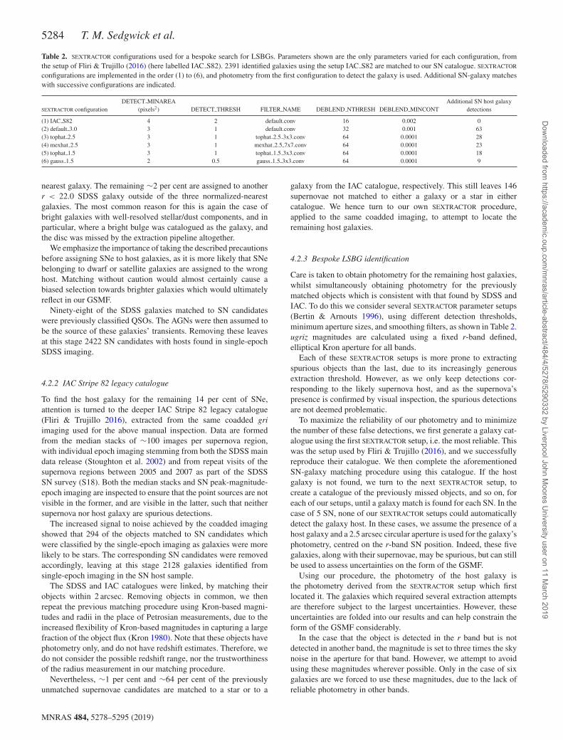
Table 2. SEXTRACTOR configurations used for a bespoke search for LSBGs. Parameters shown are the only parameters varied for each configuration, fromthe setup of Fliri & Trujillo (2016) (here labelled IAC S82). 2391 identified galaxies using the setup IAC S82 are matched to our SN catalogue. SEXTRACTOR

configurations are implemented in the order (1) to (6), and photometry from the first configuration to detect the galaxy is used. Additional SN-galaxy matcheswith successive configurations are indicated.

SEXTRACTOR configurationDETECT MINAREA

(pixels2) DETECT THRESH FILTER NAME DEBLEND NTHRESH DEBLEND MINCONTAdditional SN host galaxy

detections

(1) IAC S82 4 2 default.conv 16 0.002 0(2) default 3.0 3 1 default.conv 32 0.001 63(3) tophat 2.5 3 1 tophat 2.5 3x3.conv 64 0.0001 28(4) mexhat 2.5 3 1 mexhat 2.5 7x7.conv 64 0.0001 23(5) tophat 1.5 3 1 tophat 1.5 3x3.conv 64 0.0001 18(6) gauss 1.5 2 0.5 gauss 1.5 3x3.conv 64 0.0001 9

nearest galaxy. The remaining ∼2 per cent are assigned to anotherr < 22.0 SDSS galaxy outside of the three normalized-nearestgalaxies. The most common reason for this is again the case ofbright galaxies with well-resolved stellar/dust components, and inparticular, where a bright bulge was catalogued as the galaxy, andthe disc was missed by the extraction pipeline altogether.

We emphasize the importance of taking the described precautionsbefore assigning SNe to host galaxies, as it is more likely that SNebelonging to dwarf or satellite galaxies are assigned to the wronghost. Matching without caution would almost certainly cause abiased selection towards brighter galaxies which would ultimatelyreflect in our GSMF.

Ninety-eight of the SDSS galaxies matched to SN candidateswere previously classified QSOs. The AGNs were then assumed tobe the source of these galaxies’ transients. Removing these leavesat this stage 2422 SN candidates with hosts found in single-epochSDSS imaging.

4.2.2 IAC Stripe 82 legacy catalogue

To find the host galaxy for the remaining 14 per cent of SNe,attention is turned to the deeper IAC Stripe 82 legacy catalogue(Fliri & Trujillo 2016), extracted from the same coadded gri

imaging used for the above manual inspection. Data are formedfrom the median stacks of ∼100 images per supernova region,with individual epoch imaging stemming from both the SDSS maindata release (Stoughton et al. 2002) and from repeat visits of thesupernova regions between 2005 and 2007 as part of the SDSSSN survey (S18). Both the median stacks and SN peak-magnitude-epoch imaging are inspected to ensure that the point sources are notvisible in the former, and are visible in the latter, such that neithersupernova nor host galaxy are spurious detections.

The increased signal to noise achieved by the coadded imagingshowed that 294 of the objects matched to SN candidates whichwere classified by the single-epoch imaging as galaxies were morelikely to be stars. The corresponding SN candidates were removedaccordingly, leaving at this stage 2128 galaxies identified fromsingle-epoch imaging in the SN host sample.

The SDSS and IAC catalogues were linked, by matching theirobjects within 2 arcsec. Removing objects in common, we thenrepeat the previous matching procedure using Kron-based magni-tudes and radii in the place of Petrosian measurements, due to theincreased flexibility of Kron-based magnitudes in capturing a largefraction of the object flux (Kron 1980). Note that these objects havephotometry only, and do not have redshift estimates. Therefore, wedo not consider the possible redshift range, nor the trustworthinessof the radius measurement in our matching procedure.

Nevertheless, ∼1 per cent and ∼64 per cent of the previouslyunmatched supernovae candidates are matched to a star or to a

galaxy from the IAC catalogue, respectively. This still leaves 146supernovae not matched to either a galaxy or a star in eithercatalogue. We hence turn to our own SEXTRACTOR procedure,applied to the same coadded imaging, to attempt to locate theremaining host galaxies.

4.2.3 Bespoke LSBG identification

Care is taken to obtain photometry for the remaining host galaxies,whilst simultaneously obtaining photometry for the previouslymatched objects which is consistent with that found by SDSS andIAC. To do this we consider several SEXTRACTOR parameter setups(Bertin & Arnouts 1996), using different detection thresholds,minimum aperture sizes, and smoothing filters, as shown in Table 2.ugriz magnitudes are calculated using a fixed r-band defined,elliptical Kron aperture for all bands.

Each of these SEXTRACTOR setups is more prone to extractingspurious objects than the last, due to its increasingly generousextraction threshold. However, as we only keep detections cor-responding to the likely supernova host, and as the supernova’spresence is confirmed by visual inspection, the spurious detectionsare not deemed problematic.

To maximize the reliability of our photometry and to minimizethe number of these false detections, we first generate a galaxy cat-alogue using the first SEXTRACTOR setup, i.e. the most reliable. Thiswas the setup used by Fliri & Trujillo (2016), and we successfullyreproduce their catalogue. We then complete the aforementionedSN-galaxy matching procedure using this catalogue. If the hostgalaxy is not found, we turn to the next SEXTRACTOR setup, tocreate a catalogue of the previously missed objects, and so on, foreach of our setups, until a galaxy match is found for each SN. In thecase of 5 SN, none of our SEXTRACTOR setups could automaticallydetect the galaxy host. In these cases, we assume the presence of ahost galaxy and a 2.5 arcsec circular aperture is used for the galaxy’sphotometry, centred on the r-band SN position. Indeed, these fivegalaxies, along with their supernovae, may be spurious, but can stillbe used to assess uncertainties on the form of the GSMF.

Using our procedure, the photometry of the host galaxy isthe photometry derived from the SEXTRACTOR setup which firstlocated it. The galaxies which required several extraction attemptsare therefore subject to the largest uncertainties. However, theseuncertainties are folded into our results and can help constrain theform of the GSMF considerably.

In the case that the object is detected in the r band but is notdetected in another band, the magnitude is set to three times the skynoise in the aperture for that band. However, we attempt to avoidusing these magnitudes wherever possible. Only in the case of sixgalaxies are we forced to use these magnitudes, due to the lack ofreliable photometry in other bands.

MNRAS 484, 5278–5295 (2019)

Dow

nlo

aded fro

m h

ttps://a

cadem

ic.o

up.c

om

/mnra

s/a

rticle

-abstra

ct/4

84/4

/5278/5

290332 b

y L

iverp

ool J

ohn M

oore

s U

niv

ers

ity u

ser o

n 1

1 M

arc

h 2

019


Figure 3. Galaxy number densities as a function of Kron r-band magnitudecalculated from a bespoke search of IAC Stripe 82 legacy coadded imagingfor SN host galaxies. Galaxies selected using our SN sample are shown inblack; in blue, the same but only including galaxies known from the IACStripe 82 legacy catalogue; in green, the same but only including galaxiesknown from the SDSS Stripe 82 galaxy catalogue.

Row 2 of Fig. 2 shows example IAC Stripe 82 legacy coaddedimaging in which the supernova is centred on a newly identifiedLSBG from our bespoke search. Uncatalogued SN hosts weremissed by the SDSS and IAC catalogues due to (i) low surfacebrightness alone; (ii) a bright neighbour; or (iii) being a close-insatellite or the lower luminosity constituent of a merger.

The different SEXTRACTOR setups shown in Table 2 were foundto overcome different problems faced by the SDSS/IAC extractionpipelines. For instance, a ‘Mexican hat’-type smoothing filter wasparticularly useful for identifying dwarf satellite galaxies close tobrighter companions.

4.2.4 Summary

For the same reasons given for a galaxy being missed by theSDSS and IAC catalogues, we find that ∼2 per cent of hostswere incorrectly identified by S18. The vast majority of galaxiesconstituting this 2 per cent are more massive than the true SNhost, and thus their inclusion in our galaxy sample would cause anunderestimation of dwarf galaxy counts.

Fig. 3 shows the galaxy magnitude distributions of the 3 SN-matched catalogues presented in this work, giving a clear compar-ison of their depth. Recall that the SDSS sample was selected toinclude only r < 22.0 (extinction-corrected) galaxies. Thus, the bestdirect comparison of r-band magnitude depth is between the IACdata set and that of the present work. The (90th, 99th) percentilesof galaxy counts come at r-band magnitudes of (22.0, 23.8) for theIAC sample and (22.8, 25.3) for our bespoke sample, respectively.

We are able to test the success of our galaxy matching by using arelationship between Galactic extinction-corrected SN peak appar-ent magnitude (rSN,peak) and redshift. Fig. 4 shows this relationshipfor those SNe matched to a galaxy for which spectroscopic redshift(zspec) is known. Redshift is plotted as ζ = ln (1 + z) (Baldry2018). For Type Ia SNe, there is an approximate maximum SNredshift as a function of SN peak apparent magnitude. CCSNe do

Figure 4. SN host galaxy spectroscopic redshift, expressed as ζ spec =ln(1 + zspec), versus supernova peak r-band apparent magnitude (rSN,peak),corrected for Galactic extinction. Black circles represent host galaxieswith �χ2

zspec> 0.4, representing more confident redshift estimates. Grey

circles represent host galaxies with spectroscopic redshifts not satisfyingthis criterion. The dashed red line is the inferred line of maximum redshift asa function of rSN,peak, used to assess the validity of host galaxy identification.

not exhibit a relationship that is sufficiently sharp to set a strictmaximum redshift, but still follow the same underlying distributionin rSN,peak–ζ space. We can hence test if a galaxy match is reasonableby verifying that the galaxy spectroscopic redshift lies below themaximum redshift expected for that supernova.

For all host galaxies with redshifts exceeding their predictedmaximum, given by the red demarcation line in Fig. 4, we performfurther inspection of the coadded imaging, to check for incorrectidentification of SN hosts. However, in no case do we find a moresensible host galaxy according to this extra criterion.

Not only can Fig. 4 be used to test galaxy matches, it can also beused as a further check that all of our transient objects are indeedSNe. The demarcation line implies that the maximum redshift forthe faintest SNe in our bespoke sample, at rSN,peak = 21.8, is z =0.48. This is hence the maximum trustworthy redshift for SNe inour sample. Bolton et al. (2012) classify objects as QSOs fromtheir spectra. Cross-matching classifications with our host galaxies,we find a sudden rise in QSO classification at z = 0.48, with�80 per cent of z > 0.48 galaxies classified as QSOs. We thusremove from the SN sample 83 transients assigned to a galaxy withzspec > 0.48, citing the fact that the transient is AGN in nature andnot an SN, leaving a final sample of 2456 host galaxies for CCSNeor Type Ia SNe.

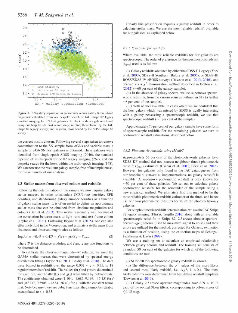
Fig. 5 shows SN-galaxy separation in arcseconds plotted againstKron galaxy magnitude. The same overall distribution is followedfor each of the three galaxy sub-samples: SDSS galaxies, IACgalaxies, and our newly identified LSBGs. SN-galaxy separationincreases towards brighter magnitudes due to the correlation ofgalaxy radius with galaxy magnitude. Normalizing separation bygalaxy radius, no correlation is found between magnitude andseparation. This helps confirm that the SN-galaxy separations foundfor our LSBGs are reasonable.

To summarize, we have successfully located the host galaxy foreach of the supernovae in the sample, with great care taken to ensure

MNRAS 484, 5278–5295 (2019)

Dow

nlo

aded fro

m h

ttps://a

cadem

ic.o

up.c

om

/mnra

s/a

rticle

-abstra

ct/4

84/4

/5278/5

290332 b

y L

iverp

ool J

ohn M

oore

s U

niv

ers

ity u

ser o

n 1

1 M

arc

h 2

019


Figure 5. SN-galaxy separation in arcseconds versus galaxy Kron r-bandmagnitude calculated from our bespoke search of IAC Stripe 82 legacycoadded imaging for SN host galaxies. In black is shown galaxies foundusing our bespoke SN host search only; in blue, those found by the IACStripe 82 legacy survey; and in green, those found by the SDSS Stripe 82survey.

the correct host is chosen. Following several steps taken to removecontamination to the SN sample from AGNs and variable stars, asample of 2456 SN host galaxies is obtained. These galaxies wereidentified from single-epoch SDSS imaging (2046), the standardpipeline of multi-epoch Stripe 82 legacy imaging (262), and ourbespoke search for the hosts within the multi-epoch imaging (148).We can now use the resultant galaxy sample, free of incompleteness,for the remainder of our analysis.

4.3 Stellar masses from observed colours and redshifts

Following the determination of the sample we now require galaxystellar masses, in order to calculate CCSN-rate densities, SFRdensities, and star-forming galaxy number densities as a functionof galaxy stellar mass. It is often useful to define an approximatestellar mass that can be obtained from absolute magnitudes andcolours (Bell et al. 2003). This works reasonably well because ofthe correlation between mass-to-light ratio and rest-frame colour(Taylor et al. 2011). Following Bryant et al. (2015), one can alsoeffectively fold in the k-correction, and estimate a stellar mass fromdistances and observed magnitudes as follows:

logM = −0.4i + 0.4D + f (z) + g(z)(g − i)obs, (8)

where D is the distance modulus, and f and g are two functions tobe determined.

To calibrate the observed-magnitude–M relation, we used theGAMA stellar masses that were determined by spectral energydistribution fitting (Taylor et al. 2011; Baldry et al. 2018). The datawere binned in redshift over the range 0.002 < z < 0.35, in 18regular intervals of redshift. The values for f and g were determinedfor each bin, and finally f(z) and g(z) were fitted by polynomials.The coefficients obtained were (1.104, –1.687, 9.193, –15.15) for f

and (0.8237, 0.5908, –12.84, 26.40) for g, with the constant termsfirst. Note because these are cubic functions, they cannot be reliableextrapolated to z > 0.35.

Clearly this prescription requires a galaxy redshift in order tocalculate stellar mass. We use the most reliable redshift availablefor our galaxies, as explained below.

4.3.1 Spectroscopic redshifts

Where available, the most reliable redshifts for our galaxies arespectroscopic. The order of preference for the spectroscopic redshift(zspec) used is as follows:

(i) Galaxy redshifts obtained by either the SDSS-II Legacy (Yorket al. 2000), SDSS-II Southern (Baldry et al. 2005), or SDSS-IIIBOSS/SDSS-IV eBOSS surveys (Dawson et al. 2013, 2016), andderived via a χ2 minimization method described in Bolton et al.(2012) (∼60 per cent of the galaxy sample).

(ii) In the absence of galaxy spectra, we use supernova spectro-scopic redshifts, from the various sources outlined in S18 (a further∼8 per cent of the sample).

(iii) With neither available, in cases where we are confident thatthe host galaxy which was missed by SDSS is tidally interactingwith a galaxy possessing a spectroscopic redshift, we use thatspectroscopic redshift (∼1 per cent of the sample).

Approximately 70 per cent of our galaxy sample have some formof spectroscopic redshift. For the remaining galaxies we turn tophotometric redshift estimations, described below.

4.3.2 Photometric redshifts using zMedIC

Approximately 65 per cent of the photometry-only galaxies haveSDSS KF method (kd-tree nearest-neighbour fitted) photometricredshift (zphot) estimates (Csabai et al. 2007; Beck et al. 2016).However, for galaxies only found in the IAC catalogue or fromour bespoke SEXTRACTOR implementations, no galaxy redshift isavailable. A supernova photometric redshift is only known for∼50 per cent of these galaxies. We set out to calculate galaxyphotometric redshifts for the remainder of the sample using anew empirical method. We ultimately find this method to be themost reliable photometric redshift estimator of the three, and henceuse our own photometric redshifts for all of the photometry-onlygalaxies.

For our photometric redshift determination, we use the IAC Stripe82 legacy imaging (Fliri & Trujillo 2016) along with all availablespectroscopic redshifts in Stripe 82. 2.5 arcsec circular-aperture-derived ugriz colours (used to maximize signal to noise) and theirerrors are utilized for the method, corrected for Galactic extinctionas a function of position, using the extinction maps of Schlegel,Finkbeiner & Davis (1998).

We use a training set to calculate an empirical relationshipbetween galaxy colours and redshift. The training set consists ofa random 50 per cent of the galaxies for which all of the followingconditions are met:

(i) SDSS/BOSS spectroscopic galaxy redshift is known.(ii) The difference between the χ2 values of the most likely

and second most likely redshift, i.e. �χ2, is >0.4. The mostlikely redshifts were determined from best-fitting redshift templates(Dawson et al. 2013).

(iii) Galaxy 2.5 arcsec aperture magnitudes have S/N > 10 ineach of the optical Sloan filters, corresponding to colour errors of�0.15 mag.

MNRAS 484, 5278–5295 (2019)

Dow

nlo

aded fro

m h

ttps://a

cadem

ic.o

up.c

om

/mnra

s/a

rticle

-abstra

ct/4

84/4

/5278/5

290332 b

y L

iverp

ool J

ohn M

oore

s U

niv

ers

ity u

ser o

n 1

1 M

arc

h 2

019


Figure 6. Spectroscopic versus photometric redshift estimates fromzMedIC, derived using 2.5 arcsec circular-aperture-derived optical galaxycolours. Redshifts are represented as ζ = ln(1 + z). The validation set of∼22 000 galaxies from the IAC Stripe 82 legacy catalogue is shown asblack circles. The validation set of ∼400 SN host galaxies found from abespoke search of the same IAC coadded imaging is shown as cyan circles.All redshifts are calculated using the zMedIC coefficients found from thetraining set of ∼22 000 galaxies. Weighted rms deviations (σ ) in ζ areindicated.

Conditions (ii) to (iii) ensure the spectroscopic redshifts andcolours we train our colour–z relation on are reliable. The resultingtraining and validation sets each consist of galaxies.

Equation (9) (below) is used to relate galaxy colours to redshift,giving each colour a coefficient. The optimal coefficients are thosewhich yield an output zphot which resembles the known zspec for ourtraining sample galaxy. The coefficients k1 and k2 in equation (9) areused as scaling values, to normalize and linearize the relationshipbetween colours and zphot. We name this code zMedIC (z Measured

via Iteration of Coefficients).

ζphot = (c1(u − g) + c2(g − r) + c3(r − i) + c4(i − z) + k1)k2 . (9)

Optimal coefficients are found by producing random sets ofnumbers to iteratively approach the set which minimizes the ζ spec

root-mean-square (rms) deviation, given by equation (10).

σ =

√

∑n

i=1 wi(ζphot − ζspec)2∑n

i=1 wi

. (10)

The weights wi are chosen to give larger weight to confident zspec

measurements and more precise colours, and to even out weightingacross redshift space. To ensure the latter, we divide the data into ζ

bins of width 0.05, normalizing weights with a value, Fbin, differentfor each bin, such that the sum of weights is the same in each bin.Thus, the final form of the weights wi is 1/(χ2

zspecFbin�(i − z)).

Due to the observed upper limit to redshift as a function of SNapparent magnitude, given by the red demarcation line in Fig. 4,we add a constraint such that the set of coefficients do not resultin more than 10 per cent of the sample lying above this redshiftlimit.

Fig. 6 shows ζ spec versus ζ phot for each r-band magnitude bin,and the corresponding values of σ for our validation set. The best-fitting coefficients of equation (9) are shown in Table 3. Note thatthis colour–z relation is trained on both star-forming and quiescent

Table 3. Best-fitting values for the coefficients in equation (9), as inferredfrom a training set of ∼22 000 galaxies, with coefficients calculatedseparately for three bins of r-band galaxy magnitude, and for the entiretraining sample (labelled ‘All’).

c1 c2 c3 c4 k1 k2

All –0.21 0.32 –0.11 –0.03 0.18 0.90r ≤ 17.5 –0.17 0.55 0.13 –0.38 0.18 1.9717.5 < r ≤ 19.5 –0.15 0.35 –0.22 –0.12 0.13 0.74r > 19.5 –0.19 0.38 –0.07 0.06 0.12 0.87

galaxies. Removing quiescent galaxies from the training set to betterreflect our SN hosts, we find no significant change to the optimalcoefficients. Furthermore, training instead on only the SN sample ofhost galaxies for which the above training set selection criteria aremet (∼400 galaxies), coefficients are similarly unaffected. We alsotest the effect of binning galaxies by r-band apparent magnitude,to check for potential improvements to σ . No benefit to σ is foundwhen dividing the large training sample of ∼22 000 galaxies intomagnitude bins, but for the much smaller sample of ∼400 CCSNhost galaxies, binning by magnitude is found to reduce σ for the r

≤ 19.5 galaxies by ∼20 per cent.The redshift parametrization of equation (9) can be modified to

deal with non-detections. The optimal coefficients are calculatedwith every possible combination of colours. For instance, if a non-detection is found for a galaxy in the g-band only, we are able touse the optimal coefficients associated with the colours (u − r), (r− i), and (i − z), in order to infer photometric redshift. The mostcommon filter with non-detections for our host galaxies is the u

band. Removing (u − g) colour increases σ by ∼20 per cent and∼2 per cent for r ≤ 19.5 and r > 19.5.

The method works over the redshift range of 0 < z < 0.4. Beyondthis upper limit, there are too few reliable spectroscopic redshiftsin our sample for an assessment, and the chosen relationship for allgalaxies may be expected to break down due to evolutionary effectsand more complex k-corrections.

To emphasize, we find that equation (9) yields the most accurateredshift estimates when using galaxy colours alone. The coefficientsused are specific to 2.5 arcsec circular-aperture colours. The rmsdeviation values between photometric and spectroscopic redshiftsfor this method are comparable to those using the SDSS KF method(Csabai et al. 2007; Beck et al. 2016), and are substantially betterthan rms deviations using an SN light-curve method (Guy et al.2007).

With redshifts estimated, we now remove likely Type Ia super-novae from our sample to leave only likely CCSNe. In Section 5.1,we compare the effects of assumptions for the nature of theunknown-type SNe. It is likely that the unknown-type fraction of thesample consists of both CCSNe and Type Ia SNe, and it is discussedhow we attempt to circumvent this problem.

4.3.3 Monte Carlo assessment of uncertainties

The CCSN-rate densities, SFRDs and hence GSMFs we will deriveare sensitive to redshift estimates in two ways: (i) galaxy stellarmasses are estimated using redshifts (see equation 8) and (ii)incompleteness of the sample is a function of redshift. Redshiftsare required to volume limit the sample. As small numbers oflog(M/M⊙) � 8.0 galaxies can significantly change the form ofthe SFRD, and hence the GSMF, we must take care when utilizingphotometric redshifts.

MNRAS 484, 5278–5295 (2019)

Dow

nlo

aded fro

m h

ttps://a

cadem

ic.o

up.c

om

/mnra

s/a

rticle

-abstra

ct/4

84/4

/5278/5

290332 b

y L

iverp

ool J

ohn M

oore

s U

niv

ers

ity u

ser o

n 1

1 M

arc

h 2

019


Figure 7. As in Fig. 6, but showing only the validation set of approximately∼22 000 IAC Stripe 82 legacy galaxies. PDFs of spectroscopic redshift asa function of photometric redshift are superimposed; these were used tomodel photometric redshift uncertainties. PDFs are calculated from a multi-Gaussian kde, in ζ phot bins of width 0.025. Redshift PDFs as a functionof photometric redshift estimation are implemented into a 1000-iterationMonte Carlo method to assess galaxy stellar mass uncertainties.

To circumvent this problem, we turn to a Monte Carlo technique.First, to assess the uncertainty in our photometric redshifts wedivide the ζ spec versus ζ phot space into bins along the ζ phot axis.We then make a histogram of counts along the ζ spec axis for eachζ phot bin, smoothed via a multi-Gaussian kernel-density estimation(kde) (Parzen 1962). As such, we have the ζ spec distribution as afunction of ζ phot. We can use each kde as a probability densityfunction (PDF) for a particular ζ spec distribution as a function ofour ζ phot input. These distributions are shown superimposed on tothe combined ζ spec versus ζ phot distribution in Fig. 7. ζ phot is foundto be systematically greater than ζ spec at the highest values (ζ phot �

0.3). The PDF is designed to statistically account for this systematicwhen implemented into the Monte Carlo technique.

We then run a 1000-iteration Monte Carlo code where eachphotometric-galaxy’s redshift is replaced by a value drawn fromthe PDFs of redshift shown in Fig. 7. For spectroscopic galaxies,the spectroscopic redshift is used, and varied for each Monte Carloiteration according to its error. For each iteration we convert agalaxy’s z-estimate to a luminosity distance assuming an h = 0.7, �m

= 0.3, �� = 0.7, flat cosmology. g and i 2.5 arcsec circular-aperture-derived magnitudes, as well as elliptical Kron-aperture-derived i-band magnitude, are varied with each iteration in accordance withtheir uncertainties. This allows an estimate of the galaxy’s stellarmass for each iteration using equation (8).

To volume limit the sample to obtain an SFRD, a z < 0.2 cut ismade following each Monte Carlo iteration. This cut is chosento limit the effects of galaxy evolution at higher redshifts, tomatch to the redshift cut of G10, for the most direct comparisonof SFRDs, and to limit the effects of extinction on SN counts.At higher redshifts, more SNe are near the detection limit of thesurvey, where a small amount of extinction can make the SNeundetectable. Limiting the number of SN detections sensitive toextinction decreases our results’ reliance on the extinction model.Using this cut, the number density of CCSNe as a function of hostgalaxy mass is estimated, with galaxy stellar mass bins 0.2 dex

Figure 8. Volumetric CCSN-rate densities (z < 0.2) as a function of hostgalaxy stellar mass. The black solid line shows galaxies derived from abespoke search for CCSN host galaxies in IAC Stripe 82 legacy imaging.The blue line shows CCSN host galaxies known from the IAC Stripe 82legacy galaxy catalogue. The green line shows CCSN host galaxies knownfrom the SDSS Stripe 82 galaxy catalogue. Shaded regions indicate the1σ of standard deviation from a Monte Carlo method and Poisson errors.The dot–dashed grey line shows the bespoke sample but with all galaxymasses derived using photometric redshifts, while the black dot–dashed lineshows all galaxy masses derived using spectroscopic redshifts (with galaxiesomitted where spectroscopic redshifts are unavailable). The grey dashed lineshows the bespoke sample but with all unknown-type SNe removed. Thegrey dotted line shows the bespoke sample but with a redshift cut of z < 0.1.

in width. We then take the mean of bin counts and the standarddeviation of bin counts over the 1000 iterations, for each bin.

5 R ESULTS AND DI SCUSSI ON

5.1 Observed CCSN-rate densities

Using equation (5), we can convert number statistics of CCSNe asa function of host galaxy stellar mass into volumetric CCSN-ratedensities, given effective SN rest-frame survey time τ and surveyvolume V. CCSN-rate densities are corrected for cosmological timedilation effects on survey time period as a function of redshift.

Fig. 8 shows volumetric z < 0.2 CCSN number densities asa function of host galaxy mass, derived from our Monte Carlotechnique. Based on the redshift cut, sky coverage and the effectivespan of the Stripe 82 SN survey [τ ∼ 270/(1 + z) d], ∼10−7 CCSNyr−1 Mpc−3 h3

70 corresponds to 1 observed CCSN. As a result, wedo not assess densities below log(M/M⊙) = 6.4, as below thismass the mean number counts per bin descend below 1 for thefull sample of galaxies found from a bespoke search for SN hostsin IAC Stripe 82 legacy imaging. For this sample we find CCSNnumber densities to decrease as a power law for log(M/M⊙) �

9.0. To show the effects of selection bias we also calculate CCSNnumber densities using only those CCSNe assigned to hosts inthe SDSS and IAC galaxy catalogues. As expected, consistencyis found at higher masses, whilst a deviation in CCSN counts isfound at lower host galaxy masses (log(M/M⊙) < 9.0) due todecreased sample completeness. A double peak in number densityis observed, consisting of a primary peak at log(M/M⊙) ∼ 10.8 and

MNRAS 484, 5278–5295 (2019)

Dow

nlo

aded fro

m h

ttps://a

cadem

ic.o

up.c

om

/mnra

s/a

rticle

-abstra

ct/4

84/4

/5278/5

290332 b

y L

iverp

ool J

ohn M

oore

s U

niv

ers

ity u

ser o

n 1

1 M

arc

h 2

019


a secondary peak at log(M/M⊙) ∼ 9.4. Using the alternative stellarmass prescription of G10 in our Monte Carlo method, a modificationof the prescription introduced by Kauffmann et al. (2003), we findthis double peak to persist.

Error bars incorporate the uncertainties in redshift and in thestellar mass parametrization, as well as the uncertainty in the natureof the unknown-type transients. We have built on the work of S18 todeduce that these objects are very likely to be supernovae. However,each of these objects could be CC or Type Ia SNe. We use volume-limited SN number statistics, calculated by R14, to derive a ratioof CCSNe to Type Ia SNe. This gives a predicted percentage ofunknown-type SNe that are Type Ia, and for each Monte Carloiteration, this percentage of unknown-type SNe, selected at random,are removed from the sample.

Fig. 8 shows the effect of removing this fraction of unknown-type SNe from the sample. Comparing with the full sample, nostrong correlation is found between the percentage of SNe thatare unknown-type and galaxy stellar mass. As such, a removalof a percentage of unknown-type SNe to attempt to remove TypeIa’s effectively corrects number densities by a constant amount,rather than modifying the CCSN-rate density distribution with mass.Changing the percentage of unknown-type SNe removed does notaffect the presence of the double peak in CCSN-rate density.

Also shown is the sub-sample of galaxies for which spectroscopicredshift is known. Lower mass galaxies are less likely to havebeen selected for spectroscopic analysis. The low-mass limit ofthe CCSN-rate density is therefore dominated by galaxies withphotometric redshifts.

To test the performance of zMedIC in producing reliable redshiftestimates, we observe the effect of calculating all galaxy massesusing our photometric redshifts. We see in Fig. 8, that zMedIC-derived redshifts, depicted by the grey dot–dashed series, are ableto reproduce the fundamental shape of the CCSN number densitiesas a function of mass, but that fine features such as the double peakare not reproduced.

Also plotted in Fig. 8 is the bespoke sample’s CCSN-rate densitiesusing a redshift cut of z < 0.1. CCSN-rate densities are increasedwhen using this cut, by a factor of ∼3. This is because we donot yet have a truly volume-limited sample, due to the supernovamagnitude cut. This draws our attention to the need for correctionsfor SN detection efficiency, ε, as discussed in Section 5.2.

To test if the double peak in observed CCSN-rate density as afunction of galaxy mass arises due to a particular SN type, we plotFig. 9, separating the CCSN sample into Type II and tType Ib/c SN.Those with spectroscopically confirmed SN types are also plottedin isolation. For all SN types and for probable and confirmed SNetypes, the double peak remains, with or without a Monte Carlovariation of masses.

5.2 Corrected CCSN-rate densities

In Section 4.1.2, we found that it is unlikely that any rSN,peak < 21.8SNe are missed by the instrumentation described in S18 over theobserving seasons, and that by locating the host galaxy for each ofthese SNe, surface brightness/mass biases are significantly reduced.However, the magnitude rSN,peak, which controls whether an SN iscontained in our sample, may be a function of redshift, the typeof CCSN that we are observing, and, most importantly for thisanalysis, host galaxy stellar mass.

(i) In the case of galaxy mass, higher mass galaxies may containmore dust than lower mass galaxies. G10 uses the Balmer decrement

Figure 9. As Fig. 8, but also showing the full CCSN host sample subdividedinto probable/confirmed CCSNe (grey dashed) and confirmed CCSNe only(grey dotted), where probable indicates those classified via photometry only,and where confirmed indicates those classified via spectroscopy. These seriesare subdivided further by SN type: probable/confirmed and confirmed TypeII SN (red dashed, red dotted) and probable/confirmed and confirmed TypeIb/c SN (yellow dashed, yellow dotted).

to estimate the dependence of AH α on galaxy stellar mass. We testthe assumption that rest-frame r-band extinction for an SN line ofsight in its host galaxy follows the same extinction-mass relation asthe H α line. Alternatively, extinction in CCSN environments withinthese galaxies may not be so strongly dependent on the extinctioninferred from the Balmer decrement. In our sample, mean CCSNcolours at peak epoch do not show any notable correlation with hostmass. For Type Ia SNe, which are known to peak at approximatelythe same (B − V) colour (Nugent, Kim & Perlmutter 2002),there is no correlation between colour and host mass (althoughenvironments may differ for Type Ia and CCSNe).

(ii) In the case of redshift, CCSNe will be fainter with distancedue to inverse square dimming to flux. They will also generallyexperience additional dimming to r-band magnitude with redshift,in our low-redshift regime, due to the shape of their spectra. k-corrections are therefore necessary to represent the higher redshiftportion of the sample correctly. CCSN k-corrections are estimatedusing a Type IIP template spectrum from Gilliland, Nugent &Phillips (1999) at peak magnitude for all SNe in our sample, andfollowing equation 1 of Kim, Goobar & Perlmutter (1996).

To investigate these effects, we consider how SN detectionefficiency depends on host galaxy mass and redshift. Using absoluter-band magnitude distributions of SNe as a function of SN type, wecan estimate the probability that each SN is brighter than rSN,peak

= 21.8, given its redshift and extinction. These probabilities leadto detection efficiencies, ε. Each CCSN contributes 1/ε counts tothe number density within its galaxy stellar mass bin, leading tocorrected CCSN-rate densities. Detection efficiencies are calculatedfor each Monte Carlo iteration to account for the uncertainties inredshift, mass and SN type that efficiencies depend on.

In order to estimate detection efficiency we first require anassumption about SN absolute magnitudes. The distributions usedare derived from the volume-limited distributions calculated byR14, who observe approximately Gaussian distributions for each

MNRAS 484, 5278–5295 (2019)

Dow

nlo

aded fro

m h

ttps://a

cadem

ic.o

up.c

om

/mnra

s/a

rticle

-abstra

ct/4

84/4

/5278/5

290332 b

y L

iverp

ool J

ohn M

oore

s U

niv

ers

ity u

ser o

n 1

1 M

arc

h 2

019


SN type. These SN types are finer classifications than made in S18:a Type II SN as classified by S18 could be any one of IIP, IIL,IIn, or IIb in R14. Therefore, if each of the four sub-types followdifferent Gaussian distributions in absolute magnitude, we assumean absolute magnitude for all Type II SNe which is the sum ofthese four Gaussians, whilst preserving the relative counts for eachsub-type. This is done similarly for Type Ib and Type Ic SNe, whichcome under ‘Type Ib/c’ in S18. The r-band absolute magnitudedistributions used are derived from the B-band distributions of R14,converted using the prescription of Jester et al. (2005) for stars withRc – Ic < 1.15. Assuming (B −V) = 0.0, as found to be typical forType Ia SNe at peak magnitude by Nugent et al. (2002), we estimatethat Mr ∼ MB + 0.1 for our CCSNe.

If the absolute magnitude distribution of an SN type can beapproximated as a Gaussian with a mean M (and standard deviationσ ), then for an individual SN of that type, the mean apparentmagnitude m as a function of redshift and extinction is given byequation (11), where krr is the r-band k-correction for the SNe, Ar,h

is the host galaxy r-band extinction and Ar,MW is the Galactic r-bandextinction along the line of sight.

m = M + 5 log dL(z) + krr + Ar,h + Ar,MW. (11)

Again, we take the sum of the Gaussian distributions to obtaindistributions for Type Ib/c and Type II SNe. By integrating underthe summed Gaussian distributions, the efficiency of detection, ε,as a function of redshift and extinction, correcting for the effects ofan SN peak magnitude cut at rSN,peak = 21.8 is then estimated byequation (12), where Ni are the predicted relative numbers of eachSN type, used to weight the sum of the n Gaussians.

ǫ =1

2−

1

2∑n

i Ni

n∑

i

Nierf

(

mi − 21.8√

2σi

)

. (12)

Detection efficiency is clearly a function of SN type. We test theeffects of bias in the SN classifications of S18 by varying the ratioof types Ia, Ib/c, and II SNe in the unknown-type fraction of thesample. However, it is found that any effects are of second-orderimportance. Therefore, we simply assume that the unknown-typeSNe follow the volume-limited type ratios of R14.

For each Monte Carlo iteration, unknown-type SNe are reas-signed an SN type, and are thus either removed from the sampleas a Type Ia, or are given an absolute magnitude drawn from thedistribution associated with either a Type Ib/c or Type II SN, whichenables an estimate of their detection efficiency for each iteration.

Equations (11) and (12) are sensitive to assumptions for hostgalaxy extinction, Ar,h. Significant uncertainty exists around therelationship between CCSN extinction and host galaxy mass. Fig. 10shows corrected CCSN-rate density versus redshift, for differentvalues of Ar,h. In comparison to the observed values, clearly thereare larger corrections at higher redshift and with higher assumedAr,h.

Also shown in Fig. 10 is the inferred CCSN-rate density derivedfrom the star formation history of Madau & Dickinson (2014),assuming different values for R, the expected number of starsthat explode as CCSNe per unit mass of stars formed. Madau &Dickinson (2014) assume a Salpeter IMF for the star formationhistory. Using this IMF with initial masses 0.1–100 M⊙ andassuming that all stars with initial masses 8–40 M⊙ result inCCSNe, then logR = −2.17. We find that using values of Ar,h from∼0.3 to 0.6 reproduces the evolution of CCSN density with redshift,with logR in the range −2.2 to −1.8. We adopt logR = −1.9.

Figure 10. Volumetric CCSN-rate density versus redshift, calculated inredshift bins of 0.05, and as a function of SN detection efficiency corrections.The grey shaded region depicts observed CCSN-rate densities from ourCCSN sample, uncorrected for SN detection efficiencies, bounded by 1σ

Poisson + Monte Carlo + Cosmic Variance errors. Colour-shaded densityvalues are corrected for SN detection efficiency. The colour bar represents thedifferent corrected CCSN rates obtained when assuming different values ofCCSN host galaxy extinction, Ar,h. Dashed lines represent expected CCSN-rate histories derived from the star formation history of Madau & Dickinson(2014), assuming different values of log R in the range –1.6 to –2.4 (see thetext). Triangular, square, and circular points represent CCSN-rate densitiesobtained by Li et al. (2011), Taylor et al. (2014), and Botticella et al. (2008),respectively. The red point shows how our observed z < 0.05 SN counts arereduced when objects inferred to have peak absolute magnitudes >−15 arediscounted as CCSNe.

Note though that the measured z < 0.05 rate is higher thanexpected. We find that there is a significant excess of SNe withvery faint peak r-band absolute magnitudes (Mr,sn > −15), onlyfound for this redshift bin. R14 predict the fraction of CCSNe withMr,sn > −15 to be negligible. One explanation for this excess couldbe a contamination of the SN sample at these lowest redshifts fromoutbursts of Luminous Blue Variables, which can exhibit similarlight-curve properties to Type IIn supernovae (see e.g. Goodrichet al. 1989; Van Dyk et al. 2000). The red point of Fig. 10 showsthe effect of removing objects inferred to have Mr,sn > −15 on thez < 0.05 CCSN counts. This corrected value is in agreement withLi et al. (2011) and Taylor et al. (2014).

The effects of corrections for SN detection bias on CCSN numberdensities as a function of galaxy stellar mass are shown in Fig. 11(with Ar,h = 0.5). CCSN-rate densities (z < 0.2) are now higherthan the uncorrected values by a factor of ∼2 at the low-mass limit,and by a factor of ∼3 at log(M/M⊙) = 10.6, the position of theprimary peak. Even though host galaxy extinction is set constantwith galaxy stellar mass, this larger factor at higher masses indicatesthe effects of a weak SN-type dependence on galaxy stellar mass.

The uncertainties take account of the efficiency correctionsin Fig. 11. Even with these uncertainties, corrected CCSN-ratedensities using the full sample of CCSN hosts show a power-lawdecrease with decreasing stellar mass, down to the low-mass limit ofthe sample. This is not evident from the samples that do not use the

MNRAS 484, 5278–5295 (2019)

Dow

nlo

aded fro

m h

ttps://a

cadem

ic.o

up.c

om

/mnra

s/a

rticle

-abstra

ct/4

84/4

/5278/5

290332 b

y L

iverp

ool J

ohn M

oore

s U

niv

ers

ity u

ser o

n 1

1 M

arc

h 2

019


Figure 11. Volumetric z < 0.2 CCSN-rate densities as a function of hostgalaxy stellar mass, corrected for the effects of SN detection efficiencies.All series are as described in Fig. 8. All results assume constant host galaxyextinction with mass, Ar,h = 0.5 mag, except the black dotted line whichassumes polynomially increasing host galaxy extinction with mass (as inG10). The grey solid line and shaded region represent CCSN-rate densitiesuncorrected for SN detection efficiencies and their 1σ errors, respectively.

bespoke LSBG detections. The 1σ levels indicated by the shadedregions suggest non-zero number densities from single-epoch SDSSimaging only down to log(M/M⊙) = 7.2, and down to log(M/M⊙)= 6.8 for IAC Stripe 82 coadded imaging. The z < 0.1 densities nowapproximate the z < 0.2 densities across the mass range, indicatingthe validity of corrections.

The black dotted line of Fig. 11 shows CCSN-rate densitiesassuming increasing extinction with mass as in G10. High-masscounts appear to be significantly overestimated compared to pre-dictions for the SFRD (see Section 5.3). This discrepancy is notsurprising because G10 uses the Balmer decrement and we expectthis to be an overestimate of typical CCSN extinction for tworeasons: (i) Balmer line production is weighted towards higherluminosity stars, and therefore younger phases of star clusters(∼1–5 Myr, G10); (ii) SNe occur at the end of a star’s life, countsare weighted by number in the IMF, and therefore SNe typicallyoccur later in the life of star clusters (∼10–40 Myr). While we stillexpect some increase of extinction with host galaxy mass due to theinterstellar medium, we assume a constant extinction with mass forthe remaining results of this work.

5.3 Star formation rate density

To convert CCSN-rate densities into SFRDs, we require an assump-tion for the CCSN rate per unit of star formation, R, as discussedin Section 2. Using a value of log R = – 1.9, we obtain theSFRDs plotted in Fig. 12, as a function of galaxy stellar mass.Our SFRDs are consistent with the G10 SFRDs (SFRtot) between9.0 < log(M/M⊙) < 11.0, the stellar mass range for which theG10 galaxy sample is expected to be complete.

Using our bespoke search for the CCSN hosts in IAC Stripe82 legacy imaging, results are sufficiently constrained to deduce apower-law decrease to SFRDs with decreasing galaxy stellar mass,down to the low-mass limit. Our method allows for an estimation

of SFRs 1.6 dex lower in stellar mass than achieved by G10, whocalculated SFRs directly from galaxy emission lines.

5.4 The galaxy stellar mass function

For the previous results of this work, no assumptions are requiredfor the volumetric numbers of galaxies at each stellar mass. Onthe contrary, by making assumptions about SSFR levels with mass,volumetric galaxy number densities as a function of mass can beestimated.

The star-forming GSMF can be derived from CCSN-rate densitiesusing equation (7), requiring an assumption for mean specificCCSN-rate variation with galaxy stellar mass (M). Specific CCSNrates are expected to trace S irrespective of M (see Section 1).CCSN rates may in fact be the most direct tracers of SFRs. Studieswhich attempt to measure both S and specific CCSN rates findconsistent slopes with M (see e.g. Graur, Bianco & Modjaz 2015).This gives confidence in our assumption of a constant R value withM, as assumed to estimate SFRDs in Section 5.3. With this similartrend in mind we can use the more numerous studies of S versusM to suggest the sensible range of assumptions for specific CCSNrate versus mass, required to derive the star-forming GSMF.

There exist conflicting results in the literature for the variationof S versus M. Whilst some studies find much higher efficienciestowards lower masses (Zheng et al. 2007; Karim et al. 2011; Li et al.2011; Graur et al. 2015), where typically S ∝ M

−0.5, others findmuch shallower trends consistent with a constant S (see e.g. Bellet al. 2007; James, Prescott & Baldry 2008; Wuyts et al. 2011, andnotably, S18).

The majority of these studies do not probe down to the massesstudied in this work. Uncertainty exists around whether the S versusM relations found for massive galaxies apply to the dwarf regimedown to log(M/M⊙) = 6.4. McGaugh et al. (2017) find a distinctstar-forming main sequence for 7 � log(M/M⊙) � 10.0, withresults consistent with a constant S. Rate simulations of Grauret al. (2015) predict a tanh-like function to specific CCSN rate withgalaxy mass, with constant specific rates in the dwarf regime andat the highest galaxy masses (>1011), and with decreasing S withincreasing mass for the masses in between.

In this work, we are most interested in the shape of the GSMF inthe dwarf regime. High-mass (log(M/M⊙) � 9.0) galaxy counts inthis work are subject to uncertainties related to the modelling of hostgalaxy extinction in massive galaxies, and the star-forming GSMFis already well constrained at high masses by several independentworks finding consistent number densities (e.g. Baldry et al. 2008;Li & White 2009; Kelvin et al. 2014). Consider instead the massrange of 8.0 < log(M/M⊙) < 9.0. The variation of SF galaxycounts with mass in this range is also well constrained, yet the effectsof varying assumptions for host galaxy extinction with mass aresignificantly smaller than at higher masses. Hence, we would expectthat the S versus M relation which produces a slope consistent withwell-constrained number densities from previous studies is the mostreliable relation.

We find the best-fitting S versus M log–log relation for 8.0 <

log(M/M⊙) < 9.0 to B12 star-forming galaxy number densities(computed from GAMA data; Driver et al. 2011) to have a slope of−0.08+0.08

−0.10. We can express equation (7) in the following form:

φSF ∝ ρCCSNM−γ . (13)

For a constant ratio of CCSN rate to SF rate with mass, ourbest-fitting S versus M slope leads to γ = 0.92+0.08

−0.10. We find aconstant value of γ with mass is able to give good agreement with

MNRAS 484, 5278–5295 (2019)

Dow

nlo

aded fro

m h

ttps://a

cadem

ic.o

up.c

om

/mnra

s/a

rticle

-abstra

ct/4

84/4

/5278/5

290332 b

y L

iverp

ool J

ohn M

oore

s U

niv

ers

ity u

ser o

n 1

1 M

arc

h 2

019


Figure 12. Volumetric z < 0.2 SFRDs as a function of host galaxy stellar mass. The black line depicts galaxies selected from a bespoke search for CCSN hostgalaxies in IAC Stripe 82 legacy imaging. The blue line shows galaxies from the IAC Stripe 82 legacy galaxy catalogue. The green line shows galaxies fromthe SDSS Stripe 82 galaxy catalogue. Shaded regions indicate 1σ of standard deviation from Monte Carlo, Poisson, and cosmic variance errors. The grey linedepicts the same as the black solid line but uncorrected for SN detection efficiencies. The magenta dotted line indicates G10 ‘SFRtot’ SFRDs.

Figure 13. The z < 0.2 star-forming GSMF, as a function of the parameterγ (R,S). The black line shows the GSMF-derived assuming constant specificCCSN rate with stellar mass, i.e. γ = 1.0. The solid region shows star-forming galaxy number densities corresponding to the 1σ uncertainty levelon the best-fitting value of γ to the B12 star-forming GSMF (the cyandashed line) in the range 8.0 < log(M/M⊙) < 9.0. The hatched regionshows number densities derived using lower values of γ .

B12 star-forming galaxy number densities, across their full range ofmasses. We show the effects of different values of γ on the derivedstar-forming GSMF in Fig. 13. This shows the typical range for Sversus M found in the literature.

Given our focus is on low-mass galaxies, we assume constantS with mass (γ = 1.0), and normalize number densities to thoseof B12 in the mass range 8.0 < log(M/M⊙) < 9.0, to derivethe star-forming galaxy number densities (Mpc−3 dex−1) for 6.4< log(M/M⊙) < 11.8. This is shown in Fig. 14 with the MonteCarlo, Poisson and cosmic variance uncertainties. We once moreshow the results based on the three galaxy samples derived usingSDSS Stripe 82 galaxies, IAC Stripe 82 legacy galaxies, and thosefrom our bespoke SN host search of IAC Stripe 82 legacy imaging.

Using the full sample of CCSN host galaxies, we observe acontinuation of a power-law rise in galaxy number density withdecreasing mass. When selecting host galaxies from the IACand SDSS catalogues, incompleteness is found below masses oflog(M/M⊙) ∼ 9.0, and zero number densities cannot be ruledout below masses of log(M/M⊙) = 6.8 and log(M/M⊙) = 7.2,respectively.

We find that our result for the full sample is consistent with theSchechter function fit to B12 star-forming galaxy number densities,when extrapolating the fit below log(M/M⊙) = 8.0. B12 use afit with parameters [log (M/M⊙), φ∗/10−3 dex−1 Mpc−3, α] =[10.72, 0.71, –1.45], which is plotted in Fig. 14. For our method, us-ing γ = 1.0, we find the best-fitting parameters to be [10.54, 1.32, –1.41], obtained using a Levenberg–Marquardt algorithm applied tothe full mass range shown in Fig. 14.

We also compare with the GSMF derived from G10’s SFRDassuming constant SSFR with galaxy mass. Between 8.4 <

log(M/M⊙) < 11.0 the gradient of number densities with massis consistent with the B12 equivalent, giving support to thisassumption.

Although we show the star-forming GSMF rather than that of allgalaxies, it is expected that the low-mass population is dominatedby star-forming galaxies (B12). Therefore, by constraining the

MNRAS 484, 5278–5295 (2019)

Dow

nlo

aded fro

m h

ttps://a

cadem

ic.o

up.c

om

/mnra

s/a

rticle

-abstra

ct/4

84/4

/5278/5

290332 b

y L

iverp

ool J

ohn M

oore

s U

niv

ers

ity u

ser o

n 1

1 M

arc

h 2

019


Figure 14. The z < 0.2 star-forming GSMF: star-forming galaxy number densities as a function of stellar mass, in logarithmic units of solar mass, as derivedfrom corresponding SFRDs (see Fig. 12). The cyan dashed line represents the Schechter fit to star-forming galaxy number densities obtained by B12. Hatchedregions represent additional uncertainties on top of observational uncertainties concerning the optimal model of SSFR versus galaxy mass (see Fig. 13).

low-mass end of the star-forming GSMF we are putting strongconstraints on the form of the total GSMF. We find our low-massnumber densities to be consistent with those from the EAGLEsimulations (Schaye et al. 2015) assuming a standard �CDMcosmology. Given that a GSMF with incompleteness in the dwarfregime could be mistaken as evidence for tension with the standardcosmology, it is clear that our overcoming of surface brightness andstellar mass biases is crucial for an assessment of the sub-structureproblem. Consistency is also found with the low-mass galaxynumber densities of Wright et al. (2017), derived from a methodused to estimate and correct for surface brightness incompleteness.We find an upper limit of 0.1 dex−1 Mpc−3 at 107 M⊙ that ison the low end of their results, which do not distinguish betweenstar-forming and quenched galaxies.

6 SU M M A RY A N D C O N C L U S I O N S

Using an SNe sample (Sako et al. 2018) as pointers to their hostgalaxies, approximately 150 newly identified LSBGs have beenlocated in IAC Stripe 82 legacy coadded imaging (Fig. 2). Thisresults in a significant improvement to magnitude depth of a CCSN-selected galaxy sample (Fig. 3). A galaxy selection using a completesample of CCSNe removes surface brightness bias.

In order to estimate stellar masses of host galaxies withoutspectroscopic redshifts, we use a colour-based code, called zMedIC,that uses the strong correlations between Sloan ugriz colours andredshift. The parametrization used is shown to work for a samplecontaining both star-forming and quiescent galaxies at z < 0.4(Fig. 6). In order to assess uncertainties on CCSN-rate densitiesas a function of galaxy stellar mass, we employ a Monte Carlomethod to fold in errors on photometric redshift (Fig. 7) and ugriz

photometry. The observed CCSN-rate densities as a function of

mass are shown to peak at ∼1010.5 M⊙ and drop by a factor of∼100 down to 106.5 M⊙ (Fig. 8).

We use a model to correct CCSN-rate densities for SN detectionefficiencies (ε) that depend on host galaxy extinction, Galacticextinction, SN type (Richardson et al. 2014) and redshift. CorrectedCCSN-rate densities are consistent with expectations derived fromthe cosmic star formation history (Madau & Dickinson 2014)assuming logR ≃ −2 (Fig. 10), where R is the expected numberof stars that explode as CCSNe per solar mass of stars formed.

By assuming a value for R, the corrected CCSN-rate density asa function of stellar mass (Fig. 11) can then be scaled to the SFRD(Fig. 12). The SFRD is consistent with the emission-line derivedSFRD at high masses (Gilbank et al. 2010) but our method extendsthe measurement to lower masses. By assuming a constant SSFR(S), and scaling appropriately (to Baldry et al. 2012), we convert theSFRD to the star-forming GSMF (Fig. 14). Derived star-forminggalaxy number densities are found to rise as a power law withdecreasing galaxy stellar mass down to the lowest assessed massesof log(M/M⊙) = 6.4; and even at the lower end of our estimateduncertainties, there is no turnover in the number density of star-forming galaxies per unit log mass at least down to log(M/M⊙) ∼7.

We have demonstrated a method which significantly reducestension between observations and the simulated predictions ofgalaxy number densities derived via a standard �CDM cosmology.The lower detection limit to galaxy stellar mass for the SN methodoutlined in this paper depends on the area, depth and the observingperiod of the SN survey. A future sample derived from LSSTtime-series and coadded imaging could significantly increase thenumber of reliably identified CCSN hosts at z < 0.2. As partof this, deep multiband photometry is crucial for constrainingphotometric redshifts and stellar masses of LSBGs. This would

MNRAS 484, 5278–5295 (2019)

Dow

nlo

aded fro

m h

ttps://a

cadem

ic.o

up.c

om

/mnra

s/a

rticle

-abstra

ct/4

84/4

/5278/5

290332 b

y L

iverp

ool J

ohn M

oore

s U

niv

ers

ity u

ser o

n 1

1 M

arc

h 2

019


enable measurements to even lower masses, and future work wouldalso enable a more detailed assessment of the functional form ofR, ε, and S on the conversion from observed CCSN-rate density toSFRD and then to GSMF.

AC K N OW L E D G E M E N T S

TMS acknowledges funding from STFC and LJMU.Funding for the SDSS-II, SDSS-III, and SDSS-IV has been

provided by the Alfred P. Sloan Foundation, the National ScienceFoundation, the U.S. Department of Energy Office of Science,the National Aeronautics and Space Administration, the JapaneseMonbukagakusho, the Max Planck Society, the Higher EducationFunding Council for England, and the Participating Institutions.SDSS-IV acknowledges support and resources from the Center forHigh-Performance Computing at the University of Utah. The SDSSweb site is www.sdss.org.

SDSS-II, SDSS-III, and SDSS-IV are managed by the Astro-physical Research Consortium for the Participating Institutionsof the SDSS Collaboration including the American Museum ofNatural History, University of Arizona, Astrophysical InstitutePotsdam, University of Basel, the Brazilian Participation Group,Brookhaven National Laboratory, University of Cambridge, theCarnegie Institution for Science, Carnegie Mellon University, CaseWestern Reserve University, University of Chicago, the ChileanParticipation Group, University of Colorado Boulder, Drexel Uni-versity, Fermilab, University of Florida, the French ParticipationGroup, the German Participation Group, Harvard-Smithsonian Cen-ter for Astrophysics, Harvard University, the Institute for AdvancedStudy, Instituto de Astrofısica de Canarias, the Japan ParticipationGroup, Johns Hopkins University, the Joint Institute for NuclearAstrophysics, the Kavli Institute for Particle Astrophysics andCosmology, Kavli Institute for the Physics and Mathematics ofthe Universe (IPMU)/University of Tokyo, the Korean ScientistGroup, the Chinese Academy of Sciences (LAMOST), LawrenceBerkeley National Laboratory, Leibniz Institut fur AstrophysikPotsdam (AIP), Los Alamos National Laboratory, Max-Planck-Institut fur Astronomie (MPIA Heidelberg), Max-Planck-Institutfur Astrophysik (MPA Garching), Max-Planck-Institut fur Extrater-restrische Physik (MPE), the Michigan State/Notre Dame/JINAParticipation Group, Universidad Nacional Autonoma de Mexico,National Astronomical Observatories of China, New Mexico StateUniversity, New York University, University of Notre Dame, Ob-servatario Nacional/MCTI, Ohio State University, University ofOxford, Pennsylvania State University, University of Pittsburgh,University of Portsmouth, Princeton University, Shanghai Astro-nomical Observatory, the Spanish Participation Group, Universityof Tokyo, the United States Naval Observatory, University ofUtah, Vanderbilt University, United Kingdom Participation Group,University of Virginia, the University of Washington, University ofWisconsin, Vanderbilt University, and Yale University.

RE FER ENCES

Baldry I. K. et al., 2005, MNRAS, 358, 441Baldry I. K. et al., 2012, MNRAS, 421, 621(B12)Baldry I. K. et al., 2018, MNRAS, 474, 3875Baldry I. K., 2018, preprint(arXiv:1812.05135)Baldry I. K., Glazebrook K., Driver S. P., 2008, MNRAS, 388, 945Beck R., Dobos L., Budavari T., Szalay A. S., Csabai I., 2016, MNRAS,

460, 1371Bell E. F., McIntosh D. H., Katz N., Weinberg M. D., 2003, ApJS, 149, 289

Bell E. F., Zheng X. Z., Papovich C., Borch A., Wolf C., Meisenheimer K.,2007, ApJ, 663, 834

Bennett C. L. et al., 2013, ApJS, 208, 20Bertin E., Arnouts S., 1996, A&AS, 117, 393Bolton A. S. et al., 2012, AJ, 144, 144Botticella M. T. et al., 2008, A&A, 479, 49Botticella M. T. et al., 2017, A&A, 598, A50Botticella M. T., Smartt S. J., Kennicutt R. C., Cappellaro E., Sereno M.,

Lee J. C., 2012, A&A, 537, A132Bryant J. J. et al., 2015, MNRAS, 447, 2857Cappellaro E., Evans R., Turatto M., 1999, A&A, 351, 459Cole S. et al., 2001, MNRAS, 326, 255Conroy C., Bullock J. S., 2015, ApJ, 805, L2Crain R. A. et al., 2015, MNRAS, 450, 1937Cross N., Driver S. P., 2002, MNRAS, 329, 579Csabai I., Dobos L., Trencseni M., Herczegh G., Jozsa P., Purger N.,

Budavari T., Szalay A. S., 2007, Astron. Nachr., 328, 852Dahlen T. et al., 2004, ApJ, 613, 189Davies L. J. M. et al., 2016, MNRAS, 461, 458Dawson K. S. et al., 2013, AJ, 145, 10Dawson K. S. et al., 2016, AJ, 151, 44Driver S. P. et al., 2011, MNRAS, 413, 971Fliri J., Trujillo I., 2016, MNRAS, 456, 1359Frieman J. A. et al., 2008, AJ, 135, 338Genel S. et al., 2014, MNRAS, 445, 175Gilbank D. G., Baldry I. K., Balogh M. L., Glazebrook K., Bower R. G.,

2010, MNRAS, 405, 2594(G10)Gilliland R. L., Nugent P. E., Phillips M. M., 1999, ApJ, 521, 30Goodrich R. W., Stringfellow G. S., Penrod G. D., Filippenko A. V., 1989,

ApJ, 342, 908Graur O., Bianco F. B., Modjaz M., 2015, MNRAS, 450, 905Grogin N. A. et al., 2011, ApJS, 197, 35Gunn J. E. et al., 2006, AJ, 131, 2332Guy J. et al., 2007, A&A, 466, 11Hastings C., Mosteller F., Tukey J. W., Winsor C. P., 1947, Ann. Math. Stat.,

18, 413Hogg D. W., Finkbeiner D. P., Schlegel D. J., Gunn J. E., 2001, AJ, 122,

2129James P. A., Prescott M., Baldry I. K., 2008, A&A, 484, 703Jester S. et al., 2005, AJ, 130, 873Karim A. et al., 2011, ApJ, 730, 61Kauffmann G. et al., 2003, MNRAS, 341, 33Kelvin L. S. et al., 2014, MNRAS, 444, 1647Kim A., Goobar A., Perlmutter S., 1996, PASP, 108, 190Kirby E. N., Cohen J. G., Guhathakurta P., Cheng L., Bullock J. S., Gallazzi

A., 2013, ApJ, 779, 102Kron R. G., 1980, ApJS, 43, 305Law N. M. et al., 2009, PASP, 121, 1395Li C., White S. D. M., 2009, MNRAS, 398, 2177Li W., Chornock R., Leaman J., Filippenko A. V., Poznanski D.,

Wang X., Ganeshalingam M., Mannucci F., 2011, MNRAS, 412,1473

Lupton R., Gunn J. E., Ivezic Z., Knapp G. R., Kent S., 2001, in HarndenF. R., Jr., Primini F. A., Payne H. E., eds, ASP Conf. Ser. Vol. 238,Astronomical Data Analysis Software and Systems X. Astron. Soc. Pac.,San Francisco, p. 269

Madau P., Dickinson M., 2014, ARA&A, 52, 415Maund J. R., 2017, MNRAS, 469, 2202McGaugh S. S., Schombert J. M., Lelli F., 2017, ApJ, 851, 22Miluzio M. et al., 2013, A&A, 554, A127Moore B., Ghigna S., Governato F., Lake G., Quinn T., Stadel J., Tozzi P.,

1999, ApJ, 524, L19Noeske K. G. et al., 2007, ApJ, 660, L43Nugent P., Kim A., Perlmutter S., 2002, PASP, 114, 803Parzen E., 1962, Ann. Math. Stat., 33, 1065Pasquali A., van den Bosch F. C., Mo H. J., Yang X., Somerville R., 2009,

MNRAS, 394, 38Pearson W. J. et al., 2018, A&A, 615, A146

MNRAS 484, 5278–5295 (2019)

Dow

nlo

aded fro

m h

ttps://a

cadem

ic.o

up.c

om

/mnra

s/a

rticle

-abstra

ct/4

84/4

/5278/5

290332 b

y L

iverp

ool J

ohn M

oore

s U

niv

ers

ity u

ser o

n 1

1 M

arc

h 2

019

http://www.sdss.org

http://dx.doi.org/10.1111/j.1365-2966.2005.08799.x

http://dx.doi.org/10.1111/j.1365-2966.2012.20340.x

http://dx.doi.org/10.1093/mnras/stx3042

http://arxiv.org/abs/1812.05135

http://dx.doi.org/10.1111/j.1365-2966.2008.13348.x

http://dx.doi.org/10.1093/mnras/stw1009

http://dx.doi.org/10.1086/378847

http://dx.doi.org/10.1086/518594

http://dx.doi.org/10.1088/0067-0049/208/2/20

http://dx.doi.org/10.1051/aas:1996164

http://dx.doi.org/10.1088/0004-6256/144/5/144

http://dx.doi.org/10.1051/0004-6361:20078011

http://dx.doi.org/10.1051/0004-6361/201629432

http://dx.doi.org/10.1051/0004-6361/201117343

http://dx.doi.org/10.1093/mnras/stu2635

http://dx.doi.org/10.1046/j.1365-8711.2001.04591.x

http://dx.doi.org/10.1088/2041-8205/805/1/L2

http://dx.doi.org/10.1093/mnras/stv725

http://dx.doi.org/10.1046/j.1365-8711.2002.05052.x

http://dx.doi.org/10.1002/asna.200710817

http://dx.doi.org/10.1086/422899

http://dx.doi.org/10.1093/mnras/stw1342

http://dx.doi.org/10.1088/0004-6256/145/1/10

http://dx.doi.org/10.3847/0004-6256/151/2/44

http://dx.doi.org/10.1111/j.1365-2966.2010.18188.x


http://dx.doi.org/10.1088/0004-6256/135/1/338


http://dx.doi.org/10.1111/j.1365-2966.2010.16640.x

http://dx.doi.org/10.1086/307549

http://dx.doi.org/10.1086/167646


http://dx.doi.org/10.1088/0067-0049/197/2/35

http://dx.doi.org/10.1086/500975

http://dx.doi.org/10.1051/0004-6361:20066930

http://dx.doi.org/10.1214/aoms/1177730388

http://dx.doi.org/10.1086/323103

http://dx.doi.org/10.1051/0004-6361:20079100

http://dx.doi.org/10.1086/432466

http://dx.doi.org/10.1088/0004-637X/730/2/61

http://dx.doi.org/10.1046/j.1365-8711.2003.06291.x


http://dx.doi.org/10.1086/133709

http://dx.doi.org/10.1088/0004-637X/779/2/102

http://dx.doi.org/10.1086/190669

http://dx.doi.org/10.1086/648598

http://dx.doi.org/10.1111/j.1365-2966.2009.15268.x

http://dx.doi.org/10.1111/j.1365-2966.2011.18162.x

http://dx.doi.org/10.1146/annurev-astro-081811-125615


http://dx.doi.org/10.3847/1538-4357/aa9790

http://dx.doi.org/10.1051/0004-6361/201321192

http://dx.doi.org/10.1086/312287

http://dx.doi.org/10.1086/517926

http://dx.doi.org/10.1086/341707

http://dx.doi.org/10.1214/aoms/1177704472

http://dx.doi.org/10.1111/j.1365-2966.2008.14233.x

http://dx.doi.org/10.1051/0004-6361/201832821


Perley D. A. et al., 2016, ApJ, 830, 13Perlmutter S. et al., 1999, ApJ, 517, 565Pier J. R., Munn J. A., Hindsley R. B., Hennessy G. S., Kent S. M., Lupton

R. H., Ivezic, Z., 2003, AJ, 125, 1559Postman M. et al., 2012, ApJS, 199, 25Richardson D., Jenkins Robert L. I., Wright J., Maddox L., 2014, AJ, 147,

118(R14)Sako M. et al., 2018, PASP, 130, 064002(S18)Schaye J. et al., 2015, MNRAS, 446, 521Schlegel D. J., Finkbeiner D. P., Davis M., 1998, ApJ, 500, 525Skillman E. D., 2005, New Astron. Rev., 49, 453Smartt S. J., 2009, ARA&A, 47, 63Smith N., Tombleson R., 2015, MNRAS, 447, 598Smith J. A. et al., 2002, AJ, 123, 2121Speagle J. S., Steinhardt C. L., Capak P. L., Silverman J. D., 2014, ApJS,

214, 15Stinson G. S., Dalcanton J. J., Quinn T., Kaufmann T., Wadsley J., 2007,

ApJ, 667, 170Stoll R., Prieto J. L., Stanek K. Z., Pogge R. W., 2013, ApJ, 773, 12Stoughton C. et al., 2002, AJ, 123, 485

Strolger L.-G. et al., 2015, ApJ, 813, 93Taylor M. et al., 2014, ApJ, 792, 135Taylor E. N. et al., 2011, MNRAS, 418, 1587Thomas D., Maraston C., Schawinski K., Sarzi M., Silk J., 2010, MNRAS,

404, 1775Tucker D. L. et al., 2006, Astron. Nachr., 327, 821Van Dyk S. D., Peng C. Y., King J. Y., Filippenko A. V., Treffers R. R., Li

W., Richmond M. W., 2000, PASP, 112, 1532Wang J., Deng J. S., Wei J. Y., 2010, MNRAS, 405, 2529Wright A. H. et al., 2017, MNRAS, 470, 283Wuyts S. et al., 2011, ApJ, 742, 96Xiao L., Eldridge J. J., 2015, MNRAS, 452, 2597York D. G. et al., 2000, AJ, 120, 1579Zheng X. Z., Bell E. F., Papovich C., Wolf C., Meisenheimer K., Rix H.-W.,

Rieke G. H., Somerville R., 2007, ApJ, 661, L41

This paper has been typeset from a TEX/LATEX file prepared by the author.

MNRAS 484, 5278–5295 (2019)

Dow

nlo

aded fro

m h

ttps://a

cadem

ic.o

up.c

om

/mnra

s/a

rticle

-abstra

ct/4

84/4

/5278/5

290332 b

y L

iverp

ool J

ohn M

oore

s U

niv

ers

ity u

ser o

n 1

1 M

arc

h 2

019

http://dx.doi.org/10.3847/0004-637X/830/1/13

http://dx.doi.org/10.1086/307221

http://dx.doi.org/10.1086/346138

http://dx.doi.org/10.1088/0067-0049/199/2/25

http://dx.doi.org/10.1088/0004-6256/147/5/118

http://dx.doi.org/10.1088/1538-3873/aab4e0


http://dx.doi.org/10.1086/305772

http://dx.doi.org/https://doi.org/10.1016/j.newar.2005.08.022

http://dx.doi.org/10.1146/annurev-astro-082708-101737


http://dx.doi.org/10.1086/339311

http://dx.doi.org/10.1088/0067-0049/214/2/15

http://dx.doi.org/10.1086/520504

http://dx.doi.org/10.1088/0004-637X/773/1/12

http://dx.doi.org/10.1086/324741

http://dx.doi.org/10.1088/0004-637X/813/2/93

http://dx.doi.org/10.1088/0004-637X/792/2/135

http://dx.doi.org/10.1111/j.1365-2966.2011.19536.x

http://dx.doi.org/10.1111/j.1365-2966.2010.16427.x

http://dx.doi.org/10.1002/asna.200610655

http://dx.doi.org/10.1086/317727

http://dx.doi.org/10.1111/j.1365-2966.2010.16629.x


http://dx.doi.org/10.1088/0004-637X/742/2/96


http://dx.doi.org/10.1086/301513

http://dx.doi.org/10.1086/518690

LJMU Research Onlineresearchonline.ljmu.ac.uk/id/eprint/9976/8/stz186.pdf · Numbers of dwarf...

Documents

Transcript of LJMU Research Onlineresearchonline.ljmu.ac.uk/id/eprint/9976/8/stz186.pdf · Numbers of dwarf...