Living to 100 and Beyond: New Discoveries in

Longevity Demographics

Do centenarians stop aging? Refutation of 'immortal phase' theory

Dr. Leonid A. Gavrilov, Ph.D.Dr. Natalia S. Gavrilova, Ph.D.

Center on Aging

NORC and The University of Chicago Chicago, Illinois, USA

The growing number of persons living beyond age 80 underscores the need

for accurate measurement of mortality

at advanced ages.

The first comprehensive study of mortality at advanced ages was published in

1939

A Study That Answered This Question

M. Greenwood, J. O. Irwin. BIOSTATISTICS OF SENILITY

Earlier studies suggested that the exponential

growth of mortality with age (Gompertz law) is followed by a period of

deceleration, with slower rates of mortality

increase.

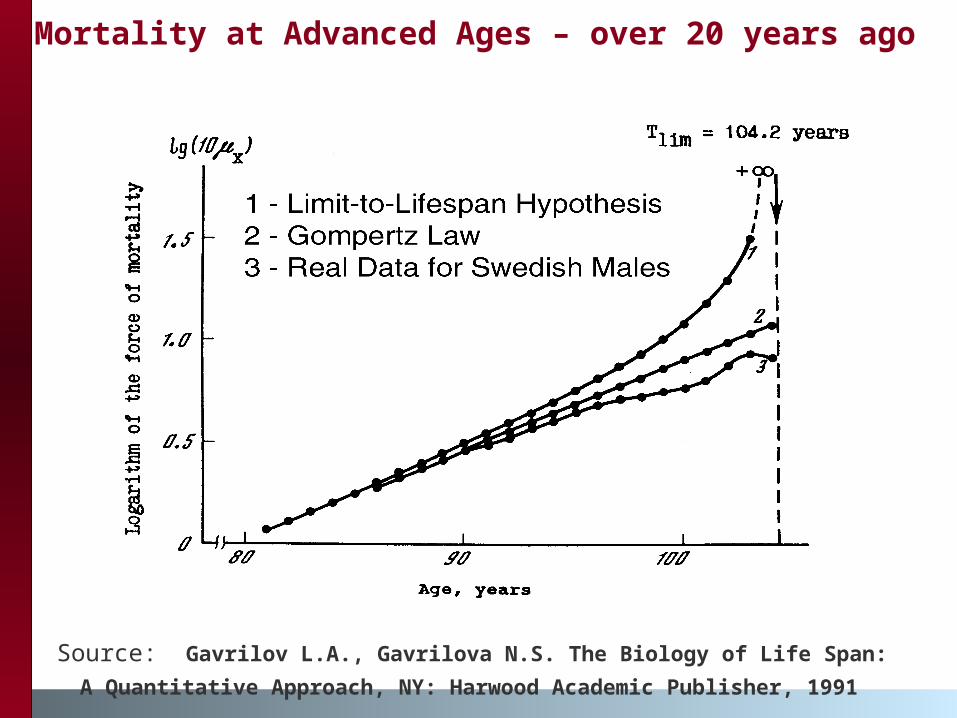
Mortality at Advanced Ages – over 20 years ago

Source: Gavrilov L.A., Gavrilova N.S. The Biology of Life Span:

A Quantitative Approach, NY: Harwood Academic Publisher, 1991

Mortality at Advanced Ages, Recent Study

Source: Manton et al. (2008). Human Mortality at Extreme Ages: Data from the NLTCS and Linked Medicare Records. Math.Pop.Studies

Existing Explanations of Mortality Deceleration

Population Heterogeneity (Beard, 1959; Sacher, 1966). “… sub-populations with the higher injury levels die out more rapidly, resulting in progressive selection for vigour in the surviving populations” (Sacher, 1966)

Exhaustion of organism’s redundancy (reserves) at extremely old ages so that every random hit results in death (Gavrilov, Gavrilova, 1991; 2001)

Lower risks of death for older people due to less risky behavior (Greenwood, Irwin, 1939)

Evolutionary explanations (Mueller, Rose, 1996; Charlesworth, 2001)

Mortality force (hazard rate) is the best indicator to study mortality at advanced

ages

Does not depend on the length of age interval

Has no upper boundary and theoretically can grow unlimitedly

Famous Gompertz law was proposed for fitting age-specific mortality force function (Gompertz, 1825)

x =

dN x

N xdx=

d ln( )N x

dx

ln( )N x

x

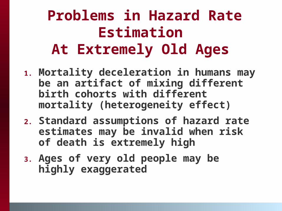
Problems in Hazard Rate Estimation

At Extremely Old Ages

1. Mortality deceleration in humans may be an artifact of mixing different birth cohorts with different mortality (heterogeneity effect)

2. Standard assumptions of hazard rate estimates may be invalid when risk of death is extremely high

3. Ages of very old people may be highly exaggerated

Social Security Administration’s Death Master File (SSA’s DMF) Helps to Alleviate the First Two

Problems

Allows to study mortality in large, more homogeneous single-year or even single-month birth cohorts

Allows to estimate mortality in one-month age intervals narrowing the interval of hazard rates estimation

What Is SSA’s DMF ?

As a result of a court case under the Freedom of Information Act, SSA is required to release its death information to the public. SSA’s DMF contains the complete and official SSA database extract, as well as updates to the full file of persons reported to SSA as being deceased.

SSA DMF is no longer a publicly available data resource (now is available from Ancestry.com for fee)

We used DMF full file obtained from the National Technical Information Service (NTIS). Last deaths occurred in September 2011.

SSA’s DMF Advantage

Some birth cohorts covered by DMF could be studied by the method of extinct generations

Considered superior in data quality compared to vital statistics records by some researchers

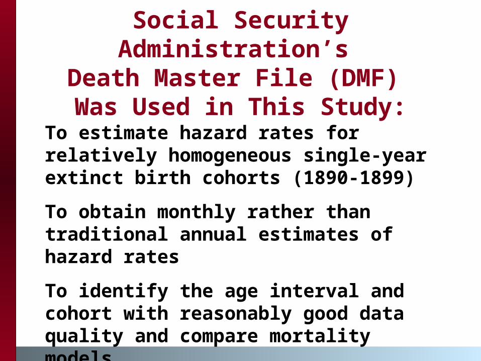
Social Security Administration’s

Death Master File (DMF) Was Used in This Study:

To estimate hazard rates for relatively homogeneous single-year extinct birth cohorts (1890-1899)

To obtain monthly rather than traditional annual estimates of hazard rates

To identify the age interval and cohort with reasonably good data quality and compare mortality models

Monthly Estimates of Mortality are More Accurate

Simulation assuming Gompertz law for hazard rate

Stata package uses the Nelson-Aalen estimate of hazard rate:

H(x) is a cumulative hazard function, dx is the number of deaths occurring at time x and nx is the number at risk at time x before the occurrence of the deaths. This method is equivalent to calculation of probabilities of death:

q x =d xl x

x = H( )x H( )x 1 =

d xn x

Hazard rate estimates at advanced ages based on DMF

Nelson-Aalen monthly estimates of hazard rates using Stata 11

More recent birth cohort mortality

Nelson-Aalen monthly estimates of hazard rates using Stata 11

Hypothesis

Mortality deceleration at advanced ages among DMF cohorts may be caused by poor data quality (age exaggeration) at very advanced ages

If this hypothesis is correct then mortality deceleration at advanced ages should be less expressed for data with better quality

Quality Control (1)Study of mortality in the states with different quality of age reporting:

Records for persons applied to SSN in the Southern states were found to be of lower quality (Rosenwaike, Stone, 2003)

We compared mortality of persons applied to SSN in Southern states, Hawaii, Puerto Rico, CA and NY with mortality of persons applied in the Northern states (the remainder)

Mortality for data with presumably different quality:

Southern and Non-Southern states of SSN receipt

The degree of deceleration was evaluated using quadratic model

Quality Control (2)

Study of mortality for earlier and later single-year extinct birth cohorts:

Records for later born persons are supposed to be of better quality due to improvement of age reporting over time.

Mortality for data with presumably different quality:

Older and younger birth cohorts

The degree of deceleration was evaluated using quadratic model

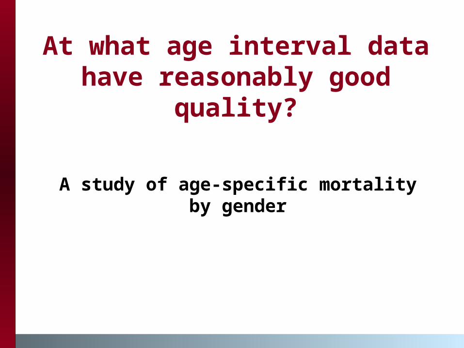
At what age interval data have reasonably good

quality?

A study of age-specific mortality by gender

Women have lower mortality at advanced ages

Hence number of females to number of males ratio should grow with age

Observed female to male ratio at advanced ages for combined 1887-1892

birth cohort

Age of maximum female to male ratio by birth cohort

Modeling mortality at advanced ages using DMF

data Data with reasonably good quality were

used: non-Southern states and 85-106 years age interval

Gompertz and logistic (Kannisto) models were compared

Nonlinear regression model for parameter estimates (Stata 11)

Model goodness-of-fit was estimated using AIC and BIC

Fitting mortality with Kannisto and Gompertz models

Akaike information criterion (AIC) to compare Kannisto and Gompertz

models, men, by birth cohort (non-Southern states)

Conclusion: In all ten cases Gompertz model demonstrates better fit than logistic model for men in age interval 85-106 years

U.S. Males

-370000

-350000

-330000

-310000

-290000

-270000

-250000

1890 1891 1892 1893 1894 1895 1896 1897 1898 1899

Birth Cohort

Aka

ike

crit

erio

nGompertz Kannisto

Akaike information criterion (AIC) to compare Kannisto and Gompertz models, women, by

birth cohort (non-Southern states)

Conclusion: In all ten cases Gompertz model demonstrates better fit than logistic model for men in age interval 85-106 years

U.S. Females

-900000

-850000

-800000

-750000

-700000

-650000

-600000

1890 1891 1892 1893 1894 1895 1896 1897 1898 1899

Birth Cohort

Akaik

e C

rite

rio

n

Gompertz Kannisto

The second studied dataset:U.S. cohort death rates taken

from the Human Mortality Database

Modeling mortality at advanced ages using HMD

data Data with reasonably good quality were

used: 80-106 years age interval Gompertz and logistic (Kannisto) models

were compared Nonlinear weighted regression model for

parameter estimates (Stata 11) Age-specific exposure values were used as

weights (Muller at al., Biometrika, 1997) Model goodness-of-fit was estimated using

AIC and BIC

Fitting mortality with Kannisto and Gompertz models, HMD U.S. data

Fitting mortality with Kannisto and Gompertz models, HMD U.S. data

Akaike information criterion (AIC) to compare Kannisto and Gompertz

models, men, by birth cohort (HMD U.S. data)

Conclusion: In all ten cases Gompertz model demonstrates better fit than logistic model for men in age interval 80-106 years

U.S.Males

-250

-230

-210

-190

-170

-150

1890 1891 1892 1893 1894 1895 1896 1897 1898 1899 1900

Birth Cohort

Aka

ike

Cri

teri

on

Gompertz Kannisto

Akaike information criterion (AIC) to compare Kannisto and Gompertz

models, men, by birth cohort (HMD U.S. data)

Conclusion: In all ten cases Gompertz model demonstrates better fit than logistic model for men in age interval 80-106 years

U.S. Females

-250-240-230-220-210-200

-190-180-170-160-150

1890 1891 1892 1893 1894 1895 1896 1897 1898 1899 1900

Birth Cohort

Akaik

e C

rite

rio

n

Gompertz Kannisto

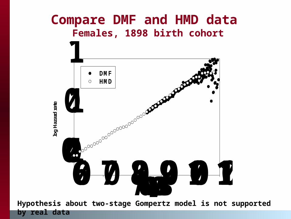
Compare DMF and HMD data Females, 1898 birth cohort

Hypothesis about two-stage Gompertz model is not supported by real data

Age, years

60 70 80 90 100 110

log

Haz

ard

rate

0.01

0.1

1

DMFHMD

Which estimate of hazard rate is the most accurate?

Simulation study comparing several existing estimates:

Nelson-Aalen estimate available in Stata Sacher estimate (Sacher, 1956) Gehan (pseudo-Sacher) estimate (Gehan, 1969) Actuarial estimate (Kimball, 1960)

Simulation study to identify the most accurate mortality

indicator Simulate yearly lx numbers assuming Gompertz

function for hazard rate in the entire age interval and initial cohort size equal to 1011 individuals

Gompertz parameters are typical for the U.S. birth cohorts: slope coefficient (alpha) = 0.08 year-1; R0= 0.0001 year-1

Focus on ages beyond 90 years Accuracy of various hazard rate estimates

(Sacher, Gehan, and actuarial estimates) and probability of death is compared at ages 100-110

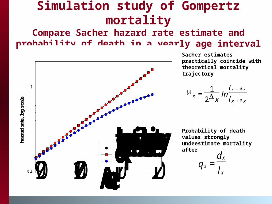
Simulation study of Gompertz mortality

Compare Sacher hazard rate estimate and probability of death in a yearly age interval

Sacher estimates practically coincide with theoretical mortality trajectory

Probability of death values strongly undeestimate mortality after age 100

Age

90 100 110 120

haza

rd r

ate,

log

scal

e

0.1

1

theoretical trajectorySacher estimateqx q x =

d xl x

x =

12x

lnl x x

l x x +

Simulation study of Gompertz mortality

Compare Gehan and actuarial hazard rate estimates

Gehan estimates slightly overestimate hazard rate because of its half-year shift to earlier ages

Actuarial estimates undeestimate mortality after age 100

x = ln( )1 q x

x

x2

+ =

2xl x l x x +

l x l x x + +

Age

100 105 110 115 120 125

haza

rd r

ate,

log

scal

e

1

theoretical trajectoryGehan estimateActuarial estimate

Deaths at extreme ages are not distributed uniformly over one-year

interval85-year olds 102-year olds

1894 birth cohort from the Social Security Death Index

Accuracy of hazard rate estimates

Relative difference between theoretical and observed values, %

Estimate 100 years 110 years

Probability of death

11.6%, understate 26.7%, understate

Sacher estimate 0.1%, overstate 0.1%, overstate

Gehan estimate 4.1%, overstate 4.1%, overstate

Actuarial estimate

1.0%, understate 4.5%, understate

Simulation study of the Gompertz mortality

Kernel smoothing of hazard rates .2

.4.6

.8H

azar

d, lo

g sc

ale

80 90 100 110 120age

Smoothed hazard estimate

Mortality of 1894 birth cohortMonthly and Yearly Estimates of Hazard

Rates using Nelson-Aalen formula (Stata)

Sacher formula for hazard rate estimation

(Sacher, 1956; 1966)

x =

1x

( )ln lx

x2

ln lx

x2

+ =

12x

lnl x x

l x x +

lx - survivor function at age x; ∆x – age interval

Hazardrate

Simplified version suggested by Gehan (1969):

µx = -ln(1-qx)

Mortality of 1894 birth cohort Sacher formula for yearly estimates of hazard

rates

What about mortality deceleration in other

species?

A. Economos (1979, 1980, 1983, 1985) found mortality leveling-off for several animal

species and industrial materials and claimed a priority in the discovery of a “non-Gompertzian paradigm of mortality”

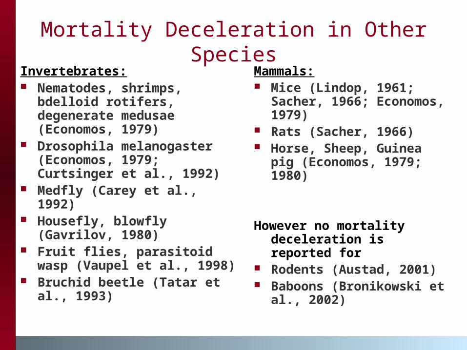
Mortality Deceleration in Other Species

Invertebrates: Nematodes, shrimps,

bdelloid rotifers, degenerate medusae (Economos, 1979)

Drosophila melanogaster (Economos, 1979; Curtsinger et al., 1992)

Medfly (Carey et al., 1992) Housefly, blowfly

(Gavrilov, 1980) Fruit flies, parasitoid wasp

(Vaupel et al., 1998) Bruchid beetle (Tatar et

al., 1993)

Mammals: Mice (Lindop, 1961;

Sacher, 1966; Economos, 1979)

Rats (Sacher, 1966) Horse, Sheep, Guinea

pig (Economos, 1979; 1980)

However no mortality deceleration is reported for

Rodents (Austad, 2001) Baboons (Bronikowski

et al., 2002)

Mortality Leveling-Off in House Fly

Musca domestica

Based on life table of 4,650 male house flies published by Rockstein & Lieberman, 1959

Age, days

0 10 20 30 40

ha

zard

ra

te,

log

sc

ale

0.001

0.01

0.1

Recent developments “none of the

age-specific mortality relationships in our nonhuman primate analyses demonstrated the type of leveling off that has been shown in human and fly data sets”

Bronikowski et al., Science, 2011

"

What about other mammals?

Mortality data for mice: Data from the NIH Interventions Testing

Program, courtesy of Richard Miller (U of Michigan)

Argonne National Laboratory data, courtesy of Bruce Carnes (U of Oklahoma)

Mortality of mice (log scale) Miller data

Actuarial estimate of hazard rate with 10-day age intervals

males females

Mortality of mice (log scale) Carnes data

Actuarial estimate of hazard rate with 10-day age intervals Data were collected by the Argonne National Laboratory, early experiments shown

males females

Bayesian information criterion (BIC) to compare the Gompertz and logistic

models, mice data

Dataset Miller dataControls

Miller dataExp., no life extension

Carnes dataEarly controls

Carnes dataLate controls

Sex M F M F M F M F

Cohort size at age one year

1281 1104 2181 1911 364 431 487 510

Gompertz -597.5 -496.4 -660.4 -580.6 -585.0 -566.3 -639.5 -549.6

logistic -565.6 -495.4 -571.3 -577.2 -556.3 -558.4 -638.7 -548.0

Better fit (lower BIC) is highlighted in red

Conclusion: In all cases Gompertz model demonstrates better fit than logistic model for mortality of mice after one year of age

Laboratory rats

Data sources: Dunning, Curtis (1946); Weisner, Sheard (1935), Schlettwein-Gsell (1970)

Mortality of Wistar rats

Actuarial estimate of hazard rate with 50-day age intervals Data source: Weisner, Sheard, 1935

males females

Bayesian information criterion (BIC) to compare logistic and Gompertz models, rat data

Line Wistar (1935)

Wistar (1970)

Copenhagen Fisher Backcrosses

Sex M F M F M F M F M F

Cohort size

1372 1407 1372 2035 1328 1474 1076 2030 585 672

Gompertz

-34.3 -10.9 -34.3 -53.7 -11.8 -46.3 -17.0 -13.5 -18.4 -38.6

logistic 7.5 5.6 7.5 1.6 2.3 -3.7 6.9 9.4 2.48 -2.75

Better fit (lower BIC) is highlighted in red

Conclusion: In all cases Gompertz model demonstrates better fit than logistic model for mortality of laboratory rats

Conclusions Deceleration of mortality in later life is more

expressed for data with lower quality. Quality of age reporting in DMF becomes poor beyond the age of 107 years

Below age 107 years and for data of reasonably good quality the Gompertz model fits mortality better than the logistic model (no mortality deceleration)

Sacher estimate of hazard rate turns out to be the most accurate and most useful estimate to study mortality at advanced ages

Acknowledgments

This study was made possible thanks to:

generous support from the

National Institute on Aging (R01 AG028620) Stimulating working environment at the Center on Aging, NORC/University of Chicago

For More Information and Updates Please Visit Our Scientific and Educational

Website on Human Longevity:

http://longevity-science.org

And Please Post Your Comments at our Scientific Discussion Blog:

http://longevity-science.blogspot.com/

Month-of-Birth and Mortality at Advanced Ages

SSA Death Master File allows researchers to study mortality in real birth cohorts by month-of-birth

Provides more accurate and unbiased estimates of life expectancy by month of birth compared to usage of cross-sectional death certificates

Month of Birth

Jan Feb Mar Apr May Jun Jul Aug Sep Oct Nov Dec

life

exp

ecta

ncy a

t ag

e 8

0,

years

7.6

7.7

7.8

7.9

1885 Birth Cohort1891 Birth Cohort