RESEARCH ARTICLE

Living on the edge: utilising lidar data to assessthe importance of vegetation structure for avian diversityin fragmented woodlands and their edges

M. Melin . S. A. Hinsley . R. K. Broughton . P. Bellamy . R. A. Hill

Received: 24 December 2017 / Accepted: 26 March 2018 / Published online: 30 March 2018

� The Author(s) 2018

Abstract

Context In agricultural landscapes, small woodland

patches can be important wildlife refuges. Their value

in maintaining biodiversity may, however, be com-

promised by isolation, and so knowledge about the

role of habitat structure is vital to understand the

drivers of diversity. This study examined how avian

diversity and abundance were related to habitat

structure in four small woods in an agricultural

landscape in eastern England.

Objectives The aims were to examine the edge effect

on bird diversity and abundance, and the contributory

role of vegetation structure. Specifically: what is the

role of vegetation structure on edge effects, and which

edge structures support the greatest bird diversity?

Methods Annual breeding bird census data for 28

species were combined with airborne lidar data in

linear mixed models fitted separately at (i) the whole

wood level, and (ii) for the woodland edges only.

Results Despite relatively small woodland areas

(4.9–9.4 ha), bird diversity increased significantly

towards the edges, being driven in part by vegetation

structure. At the whole woods level, diversity was

positively associated with increased vegetation above

0.5 m and especially with increasing vegetation

Data accessibility The lidar data used for this study isavailable from the Centre for Environmental Data Analysis athttp://www.ceda.ac.uk/. The bird data is owned and main-tained by the Centre of Ecology and Hydrology (https://www.ceh.ac.uk/).

M. Melin (&) � R. A. Hill

Department of Life and Environmental Sciences,

Bournemouth University, Talbot Campus, Fern Barrow,

Poole, Dorset BH12 5BB, UK

e-mail: mmelin@bournemouth.ac.uk

R. A. Hill

e-mail: rhill@bournemouth.ac.uk

S. A. Hinsley � R. K. Broughton

Centre for Ecology and Hydrology, Benson Lane,

Crowmarsh Gifford, Wallingford,

Oxfordshire OX10 8BB, UK

e-mail: sahi@ceh.ac.uk

R. K. Broughton

e-mail: rbrou@ceh.ac.uk

P. Bellamy

Center for Conservation Science, RSPB, The Royal

Society for the Protection of Birds (RSPB), The Lodge,

Sandy, Bedfordshire SG19 2DL, UK

e-mail: paul.bellamy@rspb.org.uk

123

Landscape Ecol (2018) 33:895–910

https://doi.org/10.1007/s10980-018-0639-7

density in the understorey layer, which was more

abundant at the woodland edges. Diversity along the

edges was largely driven by the density of vegetation

below 4 m.

Conclusions The results demonstrate that bird diver-

sity was maximised by a diverse vegetation structure

across the wood and especially a dense understorey

along the edge. These findings can assist bird conser-

vation by guiding habitat management of remaining

woodland patches.

Keywords Avian diversity � Fragmentation �Vegetation structure � Lidar � Forest edge � Habitat

structure � Edge effect � Biodiversity

Introduction

Habitat fragmentation has been shown to have nega-

tive impacts on species diversity across ecosystems

(Donald et al. 2001; Mahood et al. 2012). A common

example of a modern fragmented landscape is a

mosaic of woodland patches scattered in an agricul-

tural matrix. In such settings, fragmentation reduces

the total extent of habitat for woodland species,

increases patch isolation, and alters the habitat quality

of individual patches, for example by changing the

physical characteristics, including edge to interior

ratios (Fuller 2012). Birds have been widely studied in

this context because of the correlation demonstrated

between their diversity and overall biodiversity (Kati

et al. 2004; Gregory and van Strien 2010). Much

previous work has shown direct effects of habitat

fragmentation on bird distributions, abundance, diver-

sity and reproductive success (Hinsley et al. 1996;

Rodriguez et al. 2001; Turcotte and Desrochers 2003;

Hinsley et al. 2009).

Bird diversity in fragmented woodland is influ-

enced by the area, structure and composition of the

woods themselves and by the configuration of the

surrounding landscape (Opdam et al. 1985; Hinsley

et al. 1995; Fletcher et al. 2007). Woodland edge

habitat can provide resources such as nest sites for

birds that typically forage in more open and agricul-

tural landscapes (Benton et al. 2003; Fahrig et al.

2011; Wilson et al. 2017). In addition, the presence of

connecting landscape features such as hedgerows and

tree lines can offer additional habitat, cover and

dispersal corridors for a range of species (Hinsley et al.

1995; Fuller et al. 2001). Partly due to these reasons,

but also strongly influenced by vegetation structure

(Fuller 1995; Batary et al. 2014), higher densities of

some bird species may be recorded at forest edges

(Schlossberg and King 2008; Knight et al. 2016).

The influence of vegetation structure across forest

edges has been investigated using conventional field

methods, such as ground-based vegetation and bird

surveys, and more recently with remote sensing

techniques. For example, in the Czech Republic,

Hofmeister et al. (2017) assessed the role of fragment

size, edge distance and tree species composition on

bird communities using aerial imagery and land cover

maps and found that both distance to the woodland

edge and tree species composition had significant

effects for majority of common bird species. In

Canada, Wilson et al. (2017) used high-resolution

aerial imagery and documented positive relationships

between the presence of linear woody features and

bird diversity among the forest-edge communities

(models including the linear woody features were

ranked best). In contrast, Duro et al. (2014) found low

or moderate relationships between Landsat imagery

based predictors and patterns of bird diversity in an

agricultural environment (R2 values between 0.28 and

0.3 for Landsat TM predictors and avian beta and

gamma diversity). Thus, the drivers of diversity in

fragmented woodlands, and especially in relation to

edge habitat, may be too fine-scaled to be studied

without sufficient consideration of the structural

composition of vegetation.

While field methods and remote sensing imagery

are limited in their ability to estimate the three-

dimensional (3D) structure of vegetation, airborne

laser scanning (ALS), utilising light detection and

ranging (lidar), is ideal for this. The first studies to use

lidar to characterize wildlife habitats were conducted

on songbirds in the UK (Hinsley et al. 2002; Hill et al.

2004). Since then, the literature has grown consider-

ably with many reviews showing the usefulness of

lidar data in wildlife studies across different land-

scapes (e.g., Bradbury et al. 2005; Vierling et al. 2008;

Davies and Asner 2014; Hill et al. 2014), and

investigating data fusion and specific metrics with

which lidar could assist in habitat modelling (Vogeler

and Cohen 2016). Recent bird studies using lidar have

assessed the effects of vegetation structure on plant,

bird and butterfly species diversity (Zellweger et al.

896 Landscape Ecol (2018) 33:895–910

123

2017), on grouse broods in boreal forests (Melin et al.

2016), and on habitat envelopes of individual forest

dwelling bird species (Vogeler et al. 2013; Hill and

Hinsley 2015; Holbrook et al. 2015; Garabedian et al.

2017).

In Britain, Broughton et al. (2012) showed that

occupation of forest edge by Marsh Tits (Poecile

palustris) was lower than in the interior, which was

associated with differences in habitat structure as

assessed using airborne lidar data. Aside from this

single species study, the technology has yet to be fully

applied to species communities in habitat refuges

within highly modified environments. This paper

combines airborne lidar data with breeding bird census

data for four small, isolated woods within an agricul-

tural landscape to: (1) quantify the edge effect on bird

species diversity in each wood; (2) determine the role

of vegetation structure in any edge effect and how this

might vary between the woods; and (3) assess how

edge structure could be managed to enhance bird

diversity and abundance in small woods.

Materials and methods

Study area

The study was conducted in Cambridgeshire, eastern

England (52�25019.300N, 0�11018.300W), where four

remnant patches of ancient woodland that once

covered the area lie within ca. 8 km2 in a landscape

dominated by intensive arable agriculture (Fig. 1).

The four woods comprise Riddy Wood (9.4 ha),

Lady’s Wood (8.4 ha) Raveley Wood (7.2 ha) and

Gamsey Wood (4.9 ha).

The woods are broadly similar in tree species

composition and structure; no wood was being

actively managed during the study period (except

maintenance of rides and control of deer populations).

All woods are dominated by Common Ash (Fraxinus

excelsior), English Oak (Quercus robur), Field Maple

(Acer campestre) and Elm (Ulmus spp.). Elm occurs in

discrete patches within each wood among an admix-

ture of the other species. The main shrub species are

Common Hazel (Corylus avellana), Hawthorn

(Crataegus spp.) and Blackthorn (Prunus spinosa),

which are well mixed and common throughout the

woods, although the exterior woodland edges are

generally dominated by Blackthorn, particularly in

Lady’s Wood and Riddy Wood. The main differences

between the four woods are related to their shape, area

and growth-stage of the forest, with the vegetation at

Lady’s Wood being generally lower than in the other

three.

All woods are located within 5–20 m above sea

level with no steep topography (e.g., hills, ridges,

ravines or other distinct topographical features) in the

near vicinity. All the woods are similarly surrounded

by an agricultural matrix and other larger woods are

located ca. 1200 m away. Individual ringed birds have

been noted to move between these woods and the

study woods, but there is no evidence for any

systematic bias in such movements.

Bird data collection

As part of a larger, long-term study, the woods were

surveyed annually in 2012–2015 to determine the

abundance and distribution of their breeding bird

populations. Each wood was visited four times per

year from late March to late July. Visits started shortly

after dawn and avoided weather conditions likely to

depress bird activity (e.g., rain and strong winds).

Birds were recorded using a spot mapping tech-

nique (Bibby et al. 1992) based on the Common Birds

Census method of the British Trust for Ornithology

(Marchant 1983). Each wood was searched systemat-

ically using a route designed to encounter all breeding

territories (Bellamy et al. 1996). Routes varied

between visits, but always included walking around

the perimeter. All birds seen or heard, and their

activity, were recorded on a map of the wood and the

mapped locations were later digitised into a GIS. Due

to the small size of the woods, and the familiarity of

the surveyors with the sites, the accuracy of the

mapping was estimated to be ca. ± 10 m. Individuals

were recorded only once, omitting any suspected

repeat observations, and only the initial location of

mobile individuals was included in analyses.

Only records of putative adults were included in the

analysis because the locations of dependent young are

not independent of their parents, and because juvenile

habitat use is not necessarily related to breeding

requirements or selection of the species concerned. In

the event, the fourth visit was omitted entirely from the

analysis because it contained a high proportion of

juvenile records. Several species were also omitted:

nocturnal species such as Owls (Strix spp.) because the

Landscape Ecol (2018) 33:895–910 897

123

census technique could not detect them reliably; game

birds because their presence/absence was influenced

by local rearing and release activities; species such as

Grey Heron (Ardea cinerea) and Mallard (Anas

platyrhynchos) which were associated with ponds;

colonially breeding species such as Jackdaws (Corvus

monedula); and ubiquitous Woodpigeons (Columba

palumbus). In total, the bird data comprised 3506

observations of 28 species (Table 1).

Airborne lidar data collection and pre-processing

The lidar data of the study area were collected with a

Leica ALS50-II laser scanning system during leaf-on

conditions on June 1st 2014. The bird survey years

(2012–2015) were selected to be close to this year to

ensure temporal compatibility with vegetation

structure (Vierling et al. 2014). Bird survey data were

not available for 2016.

The lidar sensor was mounted on a fixed-wing

aircraft flown at an altitude of ca. 1600 m with a scan

half angle of 10� and a pulse repetition frequency of

143.7 MHz, resulting in a nominal sampling density of

1.9 pulses per m2 and a footprint size of ca. 35 cm.

Due to overlapping flight lines the average sampling

density in the study area was 2.7 pulses per m2, a

density that has proven to be sufficient in describing

vegetation structure when assessing wildlife habitats

and forest structural profile in general (Hill et al. 2004;

Melin et al. 2016; Zellweger et al. 2017). The ALS50-

II device captures a maximum of four return echoes for

one emitted laser pulse with an approximate vertical

discrimination distance of 3.5 m between the echoes.

All of the echo categories were used in this study. The

Fig. 1 The study area and the four target woods displayed as Canopy Height Models, which show the top surface of the vegetation and

its height (lighter shading indicates taller vegetation)

898 Landscape Ecol (2018) 33:895–910

123

lidar echoes were classified into ground or vegetation

hits following the method of Axelsson (2000), as

implemented in LAStools software. Next, a raster

Digital Terrain Model (DTM) with a 1 m spatial

resolution was interpolated from the classified ground

hits using inverse distance weighted interpolation

(IDW). This DTM was then subtracted from the

elevation values (z-coordinates) of all the lidar returns

to scale them to above ground height.

Calculating variables of diversity and vegetation

structure

For analysis, the four woods were delineated into cells

with an area of ca. 215 m2. The cell size was chosen to

account for potential inaccuracies in bird locations and

to ensure sufficient lidar echoes within the cells to

adequately calculate the 3D metrics of vegetation

structure. The delineation was done with basic

geoprocessing tools in QGIS. Cells were constrained

to lie within the woodland boundary and hence cell

Table 1 The number of bird observations recorded from each wood by species during three survey visits in each of 4 years

(2012–2015)

Species Latin name Number of observations Total

Raveley Riddy Lady’s Gamsey

Blackbird Turdus merula 36 72 60 49 217

Blackcap Sylvia atricapilla 43 69 74 39 225

Blue tit Cyanistes caeruleus 161 217 190 137 705

Bullfinch Pyrrhula pyrrhula 3 7 18 10 38

Chaffinch Fringilla coelebs 65 108 119 64 356

Chiffchaff Phylloscopus collybita 16 28 40 17 101

Coal tit Periparus ater 18 15 8 11 52

Crow Corvus corone 7 2 1 8 18

Dunnock Prunella modularis 9 8 23 10 50

Garden warbler Sylvia borin 0 1 5 0 6

Goldcrest Regulus regulus 2 1 1 0 4

Goldfinch Carduelis carduelis 7 5 7 4 23

Great spotted woodpecker Dendrocopos major 24 30 23 16 93

Great tit Parus major 97 105 129 74 405

Green woodpecker Picus viridis 7 17 14 17 55

Jay Garrulus glandarius 4 3 8 4 19

Long-tailed tit Aegithalos caudatus 28 30 23 25 106

Magpie Pica pica 10 1 9 0 20

Marsh tit Poecile palustris 19 15 1 8 43

Nuthatch Sitta europaea 0 6 0 1 7

Robin Erithacus rubecula 72 83 119 57 331

Song thrush Turdus philomelos 1 5 5 12 23

Stock dove Columba oenas 20 36 27 12 95

Treecreeper Certhia familiaris 46 41 31 30 148

Whitethroat Sylvia communis 2 8 5 4 19

Willow warbler Phylloscopus trochilus 0 2 2 0 4

Wren Troglodytes troglodytes 51 106 129 47 333

Yellowhammer Emberiza citrinella 1 1 2 6 10

Total 749 1022 1073 662 3506

Landscape Ecol (2018) 33:895–910 899

123

shape was allowed to be irregular to ensure similar cell

areas and to fit within the irregular boundaries of the

woods. However, it was ensured that the cells,

especially along the edges, were of approximately

similar depth and shape so that differences would not

introduce any systematic bias in relation to bird

occurrence probabilities. Next, bird data (i.e., individ-

ual bird locations) and lidar data were extracted for

each cell, which formed the research setting (Fig. 2).

Lidar data were used to obtain metrics of vegetation

structure such as maximum and average canopy height

and its standard deviation, proportion of vegetation

above ground level (defined as[ 0.5 m), proportion of

vegetation at different height levels of the overstorey

(canopy) and understorey (shrub) layers, and Foliage

Height Diversity (FHD) (see Table 2). FHD was

calculated according to MacArthur and MacArthur

(1961):

FHD ¼ �X

pi � logðpiÞ ð1Þ

where pi is the proportion of lidar returns in zone i. The

FHD was derived by binning the lidar returns into

zones according to their height: 0.5–4,[ 4–8,[ 8–12,

[ 12–16,[ 16–20 and[ 20 m. The division created

six nearly equal height classes in terms of how the

proportion of vegetation was spread throughout the

vertical profile of the woods. The variable FHD has

been estimated in a similar fashion from lidar data for

bird habitat modeling in Clawges et al. (2008). The

chosen variables have proven to be attainable from

lidar data and useful in assessing vegetation structure

and bird habitats, in particular (Hill et al. 2014).

Other cell-specific metrics included the Euclidean

distance from the centroid of each cell to the nearest

woodland-field edge, and for the edge cells only, the

Euclidean distance to the nearest hedgerow and the

aspect (i.e., the slope direction or bearing), which was

calculated from the DTM. The purpose of aspect was

to assess whether, for example, south-facing edges

differ in their vegetation structure compared with

Fig. 2 Lady�s Wood delineated into grid cells, showing the cell-level bird and lidar data

900 Landscape Ecol (2018) 33:895–910

123

north-facing ones due to different light conditions or

degree of exposure. Distances to hedgerows were

included because hedges may provide hedgerow-

dwelling species with access points to the edges of

small woods (Hinsley et al. 1995). The definition

‘nearest hedgerow’ included hedges adjoined to the

woodland edge and also those within 300 m (the

maximum distance to any hedge).

Finally, indices of bird diversity were derived for

each cell as species richness (SpeciesN) calculated as

the cumulative total number of species, bird abun-

dance (BirdN) calculated as the maximum number of

individual birds encountered in a cell in any one

survey, and the Shannon index of diversity (Shannon

1948) (ShannonD). All the metrics are listed in

Table 2.

Modeling bird diversity and abundance

The aim of the modeling was to examine which

variables had the greatest effect on bird diversity and

whether or not this differed between the four woods.

Therefore, linear mixed-effects models were the

chosen method. Mixed models extend the basic linear

model such that they recognize grouped or nested

structures in data via random effects. Here, the data

were grouped into four separate woods with different

areas and structures (Pinherio and Bates 2004).

Altogether, two sets of models were fitted to the

data. The first models quantified for cells across the

whole wood the most significant predictors of bird

diversity out of those listed in Table 2. The second

models were fitted only to data from the row of cells

immediately adjacent to the edge of each wood,

corresponding to a width of approximately 14.7 m.

This was to examine what drives bird diversity along

the edge itself, i.e., establish what determines a

Table 2 The cell-specific predictor and response variables used in the analysis

Variable Description

Predictor variables

WoodID Used as the random effect as the data were grouped into four woods

FHD Foliage height diversity. Calculated from all returns using Eq. (1). FHD conveys the proportional distribution

of vegetation throughout the full vertical profile of the forest

p_veg % of lidar returns coming from above 0.5 m (vegetation hits). A p_veg value of 0.55 would mean that 55% of

returns from this cell came from above 0.5 m

p_canopy_Xa % of lidar returns coming from above X m in the vegetation profile, calculated from all the returns. A

p_canopy_8 value of 0.75 would mean that 75% of returns from this cell came from above 8 m

p_shrub_Xa % of lidar returns between 0.5 and X m, calculated only from the returns below X m. A p_shrub_4 value of

0.6 would mean that 60% of the returns coming from below 4 m within this cell hit vegetation, not the

ground

h_max Maximum height of the lidar returns per cell

h_avg, hstdev Average height of the lidar returns per cell and their standard deviation

EdgeDistance The Euclidean distance (m) from the centroid of a cell to the nearest edge

HedgeDistance 1

and 2

The Euclidean distance (m) from the centroid of a cell to the nearest hedgerow (calculated for the edge cells

only). Assessed as a continuous variable (1) and as a categorical variable (2) divided into 25 m classes, i.e.,

0–25,[ 25–50 m, etc

Aspect The slope direction of the cell (calculated for the edge cells only). Assessed as a categorical variable divided

into eight classes, i.e., north, north-east, east etc

Response variables

ShannonD The Shannon index of diversity

BirdN Bird abundance: the maximum number of individual birds observed in the cell during any single survey

SpeciesN Bird species richness: the cumulative total number of species observed within the cell

aFour cut-off values (4, 6, 8 and 10 m) were used for assessing the density of shrub- and canopy cover at different heights. This equals

to eight different variables, four for shrub cover and four for canopy cover

Landscape Ecol (2018) 33:895–910 901

123

favoured edge and how its vegetation might differ

from sections of edges that are avoided. Variable

selection was done by forward selection where the

single most significant variable was first added to the

model, after which the process was iterated until no

more variables could be added; the final model

included only significant (p\ 0.05) variables. All

modeling and analyses were conducted in R (R Core

Team 2017) using the package nlme (Pinheiro et al.

2017) and ggplot2 (Wickham 2009) for visualizations.

Package lmfor (Mehtatalo 2017) were used to examine

model residuals, which showed no non-linearity or

heteroscedasticity. Multicollinearity among the final

predictors was examined with the vis function from the

package car (Fox and Weisberg 2011), and it was

noted not to be an issue. Spatial autocorrelation (SAC)

was examined individually for each wood and it was

noted to be present in the immediate neighborhood of a

cell. This was accounted for by using a linear SAC

structure with the built-in functions available in the

nlme package.

Results

Bird diversity in the study area

The four woods differed in how many species they

supported, and in individual species abundance. The

most abundant generalists, such as the Blue Tit, Robin

and Great Tit, followed a consistent pattern where they

were less abundant in the two smaller woods (Gamsey

and Raveley) than in the two larger woods (Riddy and

Lady’s). In contrast, some edge-preferring species,

such as Yellowhammer and Whitethroat, were

encountered more often in the smallest wood (Gam-

sey) than in the others (Table 1). Bird diversity and

abundance per unit area were highest in Gamsey,

followed by Lady’s, Raveley and Riddy Woods

(Table 3).

Forest structure in the woods and their edges

The decision to group the data by wood prior to the

modeling was justified by the clear difference in the

details of their structure (Fig. 3a). Lady’s Wood is

dominated mostly by vegetation below 11 m in height

and with all trees being below 20 m. In addition,

Lady’s Wood (together with Raveley) is more open

than the other woods, as shown by a proportionally

higher number of ground echoes (class 1 in Fig. 3a).

By contrast, Gamsey Wood has the lowest proportion

of ground echoes and (together with Riddy Wood), the

tallest canopies.

The differences are further evident at the woodland

edges (Fig. 3b). Lady’s Wood is clearly different from

the other woods by having over 80% of its edge

vegetation below 7 m. Also, the edge of Lady’s Wood

is the densest, having the lowest proportion of ground

echoes (class 1 in Fig. 3b). By contrast, Raveley Wood

has the highest proportion of vegetation in the higher

canopies (above 12 m) and the lowest amount below

8 m at its edge. Raveley Wood also has the most open

edges (i.e., highest proportion of ground and near-

ground echoes—class 1 in Fig. 3b).

Drivers of bird diversity and abundance

in the woods

Three variables, EdgeDistance, p_veg and p_-

canopy_6 (Table 2), were selected as the most signif-

icant predictors in all the ‘whole wood’ models, i.e.,

for all three response variables (SpeciesN, BirdN,

ShannonD), while the amount of vegetation between

the ground and 4 m was the single most significant

predictor in the ‘edge models’ for all three response

variables (Table 4). Thus, bird diversity and abun-

dance decreased with increasing edge distance and

increased with higher amounts of vegetation (p_veg).

However, the relationships to a second variable,

p_canopy_6 (the amount of vegetation above 6 m),

were negative indicating that bird abundance and

diversity were negatively influenced by an increase in

the amount of vegetation if it took place only in the top

canopy and not at all in the shrub layer, i.e., below

6 m. Similar trends were also apparent within the

model output for woodland edges, where the hotspots

of avian abundance and diversity were the edges with

the densest shrub cover (i.e., the highest amount of

vegetation below 4 m). As all three tested bird metrics

were highly consistent in their relationships with the

predictor variables, only SpeciesN is shown for

reference in Figs. 4 and 5.

It was notable that the effects of both distance from

the woodland edge and shrub cover were consistent

between the four woods and for all the diversity

metrics, albeit varying in strength (Table 4). Gamsey

Wood, despite its smallest size, had the highest

902 Landscape Ecol (2018) 33:895–910

123

average diversity and most bird species per unit area,

followed by Lady’s, Riddy and Raveley Wood.

Similarly, the decrease in bird diversity as edge

distance increased was evident in all woods, but due to

its smallest size, the effect was the strongest in

Gamsey Wood (Table 4a). Along the edge, there was

no significant difference in bird diversity between the

woods and the relationships of the diversity metrics

were also consistent: as the amount of vegetation

below 4 m increased, so did bird abundance and

diversity (Table 4b).

Table 3 Summary statistics of the cell-level bird diversity metrics in the four woods

WoodID (and size) ShannonD BirdN SpeciesN

Avg. SD Max. Avg. SD Max. Avg. SD Max.

Riddy (9.4 ha) 0.56 0.56 2.36 1.22 0.58 6 1.93 1.60 12

Lady’s (8.4 ha) 0.62 0.59 2.15 1.33 0.58 4 2.13 1.72 9

Raveley (7.2 ha) 0.61 0.56 2.08 1.31 0.62 4 2.08 1.53 8

Gamsey (4.9 ha) 0.69 0.63 2.38 1.35 0.70 6 2.39 1.95 12

ShannonD Shannon Index, BirdN the maximum number of birds encountered during one visit, SpeciesN the number of different

species encountered, Avg. arithmetic mean, Max. the maximum value, SD standard deviation

0.00

0.05

0.10

0.15

0.20

0.25

0.30

1 2 3 4 5 6 7 8 9 10 11 12 13 14 15 16 17 18 19 20 21

% o

f ech

oes

Height bin (m)

0.00

0.02

0.04

0.06

0.08

0.10

0.12

0.14

1 2 3 4 5 6 7 8 9 10 11 12 13 14 15 16 17 18 19 20 21 22 23

% o

f ech

oes

Riddy Lady's Raveley Gamsey

(A)

(B)

Fig. 3 Histograms showing

the proportion (Y-axis) of

lidar echoes reflecting from

vegetation heights in 1 m

height bins in four whole

woods (a) and along their

edges only (b). The X-axis

shows different height bins,

where Class 1 includes

echoes below 1 m, Class 2

includes those within

1–2 m, etc. In a Class 23

includes all echoes above

22 m, and in b Class 21

includes all echoes above

20 m

Landscape Ecol (2018) 33:895–910 903

123

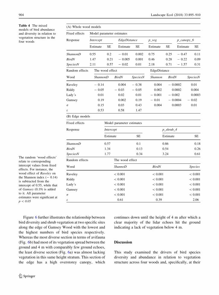
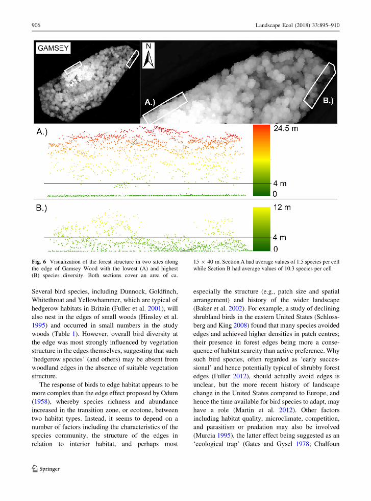
Figure 6 further illustrates the relationship between

bird diversity and shrub vegetation at two specific sites

along the edge of Gamsey Wood with the lowest and

the highest numbers of bird species respectively.

Whereas the most diverse section in terms of avifauna

(Fig. 6b) had most of its vegetation spread between the

ground and 4 m with comparably few ground echoes,

the least diverse section (Fig. 6a) was almost lacking

vegetation in this same height stratum. This section of

the edge has a high overstorey canopy, which

continues down until the height of 4 m after which a

clear majority of the lidar echoes hit the ground

indicating a lack of vegetation below 4 m.

Discussion

This study examined the drivers of bird species

diversity and abundance in relation to vegetation

structure across four woods and, specifically, at their

Table 4 The mixed

models of bird abundance

and diversity in relation to

vegetation structure in the

four woods

The random ‘wood effects’

relate to corresponding

intercept values from fixed

effects. For instance, the

wood effect of Raveley on

the Shannon index (- 0.14)

is subtracted from the

intercept of 0.55, while that

of Gamsey (0.19) is added

to it. All parameter

estimates were significant at

p\ 0.05

(A) Whole wood models

Fixed effects Model parameter estimates

Response Intercept EdgeDistance p_veg p_canopy_6

Estimate SE Estimate SE Estimate SE Estimate SE

ShannonD 0.55 0.2 - 0.01 0.002 0.75 0.25 - 0.47 0.11

BirdN 1.47 0.21 - 0.005 0.001 0.46 0.28 - 0.22 0.09

SpeciesN 2.11 0.57 - 0.02 0.01 2.18 0.71 - 1.57 0.31

Random effects The wood effect EdgeDistance

Wood ShannonD BirdN SpeciesN Shannon BirdN SpeciesN

Raveley - 0.14 0.004 - 0.38 0.004 - 0.0002 0.01

Riddy - 0.05 - 0.03 - 0.05 0.002 0.0002 0.004

Lady�s 0.01 0.02 0.01 - 0.001 - 0.002 0.0003

Gamsey 0.19 0.002 0.19 - 0.01 - 0.0004 - 0.02

r 0.15 0.03 0.43 0.004 0.0003 0.01

e 0.53 0.58 1.47

(B) Edge models

Fixed effects Model parameter estimates

Response Intercept p_shrub_4

Estimate SE Estimate SE

ShannonD 0.57 0.1 0.86 0.18

BirdN 1.34 0.13 0.54 0.26

SpeciesN 1.77 0.34 3.24 0.61

Random effects The wood effect

Wood ShannoD BirdN Species

Raveley \ 0.001 \ 0.001 \ 0.001

Riddy \ 0.001 \ 0.001 \ 0.001

Lady�s \ 0.001 \ 0.001 \ 0.001

Gamsey \ 0.001 \ 0.001 \ 0.001

r \ 0.001 \ 0.001 \ 0.001

e 0.61 0.39 2.06

904 Landscape Ecol (2018) 33:895–910

123

edges. Bird diversity and abundance were found to be

positively affected by vegetation density, and the

importance of the shrub layer for both whole woods

and the edges was also revealed. These findings were

achieved by combining lidar data with spot-mapped

bird data, which allowed the examination of the spatial

relationships between bird distributions and vegeta-

tion structure across the whole woods and in relation to

the full vegetation height profile. The capabilities of

the type of lidar data used, as well as the variables

derived from it, in characterising 3D vegetation

structure have been shown by many previous studies

(Hill et al. 2004; Broughton et al. 2012; Vogeler et al.

2013; Melin et al. 2016; Zellweger et al. 2017).

However, our results extend those of other studies

where optical remote sensing data have been used to

assess bird-edge relationships (Duro et al. 2014;

Pfeifer et al. 2017), without the advantage of 3D data

on vegetation structure. While field methods have

quantified the importance of shrub vegetation in edge-

habitats (Knight et al. 2016), lidar offers an efficient

and, due to national scanning campaigns, an increas-

ingly available method (Melin et al. 2017).

Small woods are often regarded as being composed

of ‘all edge’, but our results showed a clear edge effect

for all four woods, with a decline in bird diversity and

abundance from the edges to the centres across a

distance of 75 m or more (Fig. 4). While both the

number of species and abundance responded posi-

tively to increasing vegetation density throughout a

wood, the main driver of this response was the density

of vegetation below 6 m, i.e., within the shrub layer

(Fig. 4, Table 4a).

Vegetation density in the shrub layer was similarly

important within the edges themselves (Fig. 5), with

all the edge models selecting vegetation heights of 4 m

(variable p_shrub_4) as the single most significant

driver of bird diversity and abundance (Table 4b). The

distance to the nearest hedgerow had a mild negative

effect on bird species richness (SpeciesN), but with a

p-value of 0.07 it was dropped from the final models.

Fig. 4 Illustration of the

relationship between

EdgeDistance (a) and

p_canopy_6 (b) with species

richness (SpeciesN) in the

‘whole woods’ (all woods

combined). The grey

polygons around the lines

depict the standard errors.

EdgeDistance is the

Euclidean distance to the

nearest woodland-field edge

and p_canopy_6 is the

proportion of lidar echoes

above 6 m

Fig. 5 Illustration of the relationship between p_shrub_4 and

species richness (SpeciesN) in the woodland edges (all woods

combined). The grey polygon around the line depicts the

standard error. p_shrub_4 is the proportion of echoes from

below 4 m which hit vegetation

Landscape Ecol (2018) 33:895–910 905

123

Several bird species, including Dunnock, Goldfinch,

Whitethroat and Yellowhammer, which are typical of

hedgerow habitats in Britain (Fuller et al. 2001), will

also nest in the edges of small woods (Hinsley et al.

1995) and occurred in small numbers in the study

woods (Table 1). However, overall bird diversity at

the edge was most strongly influenced by vegetation

structure in the edges themselves, suggesting that such

‘hedgerow species’ (and others) may be absent from

woodland edges in the absence of suitable vegetation

structure.

The response of birds to edge habitat appears to be

more complex than the edge effect proposed by Odum

(1958), whereby species richness and abundance

increased in the transition zone, or ecotone, between

two habitat types. Instead, it seems to depend on a

number of factors including the characteristics of the

species community, the structure of the edges in

relation to interior habitat, and perhaps most

especially the structure (e.g., patch size and spatial

arrangement) and history of the wider landscape

(Baker et al. 2002). For example, a study of declining

shrubland birds in the eastern United States (Schloss-

berg and King 2008) found that many species avoided

edges and achieved higher densities in patch centres;

their presence in forest edges being more a conse-

quence of habitat scarcity than active preference. Why

such bird species, often regarded as ‘early succes-

sional’ and hence potentially typical of shrubby forest

edges (Fuller 2012), should actually avoid edges is

unclear, but the more recent history of landscape

change in the United States compared to Europe, and

hence the time available for bird species to adapt, may

have a role (Martin et al. 2012). Other factors

including habitat quality, microclimate, competition,

and parasitism or predation may also be involved

(Murcia 1995), the latter effect being suggested as an

‘ecological trap’ (Gates and Gysel 1978; Chalfoun

Fig. 6 Visualization of the forest structure in two sites along

the edge of Gamsey Wood with the lowest (A) and highest

(B) species diversity. Both sections cover an area of ca.

15 9 40 m. Section A had average values of 1.5 species per cell

while Section B had average values of 10.3 species per cell

906 Landscape Ecol (2018) 33:895–910

123

et al. 2002). Intensive landscape modification may,

however, dilute the ‘ecological trap’ effect by reduc-

ing predator diversity and abundance (Batary et al.

2014). At some scales, detection of strong external

edge effects may be influenced by the frequency and

distribution of internal edges. In a study of forest

fragments (maximum size 255 ha) in the Czech

Republic, Hofmeister et al. (2017) found that 60% of

the forest area was within 50 m of an edge and only

10% at more than 150 m.

In intensive agricultural landscapes of the UK, and

elsewhere in Europe, habitat edges, along with

hedgerows, may constitute the majority of the shrubby

vegetation available. Hence these habitats tend to

attract woodland species requiring dense cover for

nesting and/or foraging and open country species in

search of nest sites, as well as early successional

species. This general pattern was apparent in our study

woods; species recorded more frequently (on average)

within 40 m of the edge than elsewhere included

woodland species (Wren, Chaffinch, Long-tailed Tit,

Robin and Blackbird), open country species (Gold-

finch and Yellowhammer), and early successional

species (Garden Warbler, Whitethroat and Dunnock).

Green Woodpecker was also more frequent near

edges, which was consistent with its use of trees for

nest holes whilst mostly foraging outside of woodland.

The central areas of our study woods were not lacking

a shrub layer, but the edges had a greater density of

lower-level (i.e., below 4 m) shrub vegetation poten-

tially offering more foraging resources and greater

cover, and were accessible to the open country species

mentioned above. These kinds of ecotonal woodland

edges with relatively low bushy growth grading into

taller shrub and tree cover are generally recommended

as a management objective (Symes and Currie 2005;

Blakesley and Buckley 2010). Other studies have also

reported greater bird abundance and diversity at forest

edges and ecotones, including both internal and

external edges (Fuller 2000; Terraube et al. 2016).

Higher light intensity along unshaded bushy edges

can promote greater vegetation density with concomi-

tant greater potential to provide resources. For exam-

ple, flowering shrubs in the woodland edge may

provide important food resources in early spring and

hence increased bird usage. In our woods, Blackthorn

in flower attracted species such as tits, most notably

Marsh Tits, which are more usually associated with

mature trees. The dense structure of Blackthorn also

provided nest sites for a range of species including

Long-tailed Tit, Chaffinch, Blackcap and Dunnock,

but some of these, particularly the former two, also

foraged in mature trees within the wood. Our finding

that both bird abundance and diversity had a similar

relationship with edge distance and vegetation struc-

ture (p_canopy_6 and p_shrub_4) was consistent with

this hypothesis that the complexity of the vegetation

offers greater niche diversity (more food, cover and

nest sites supporting more individuals). Thus, wood-

land bird diversity seems to depend on the overall

structural complexity of the wood: a patch of scrub

without trees or a stand of trees lacking shrubs are both

unlikely to support the range of species typical of

structurally diverse woodland.

Previous work (Hinsley and Bellamy 1998) found

that the co-occurrence of greater species richness and

the abundance of individual bird species in small

woods were influenced by their connectivity, the

number of habitat types present within a wood and the

density of vegetation in the shrub layer. The present

study highlights the importance of the woodland edge

in providing dense shrubby vegetation. Large tracts of

woodland can contain complex networks of rides and

glades with shrubby edge vegetation whilst retaining

the overall essential structure of closed canopy

woodland. In contrast, small woods are too small to

support extensive internal structures without becom-

ing disjointed, i.e., more open habitat with a greater

resemblance to scrub than woodland. Thus, the

external edges of small woods are a valuable resource,

and especially so in intensive arable landscapes where

the contrast between the patches of semi-natural

habitat and the cropland tends to be abrupt and stark.

Although there seem to be few genuinely edge-

dependent bird species, this may be largely a matter of

how ‘edge’ is interpreted. For example, Skylarks

(Alauda arvensis) and Meadow Pipits (Anthus praten-

sis) using mosaic habitats of heather and grassland

would not usually be described as edge species,

whereas Black Grouse (Tetrao tetrix) using complexes

of woodland and moorland may be (Watson and Moss

2008). In fragmented forest, Holbrook et al. (2015)

found both the area of harvested forest and vegetation

structure influenced site occupancy of red-naped

sapsuckers (Sphyrapicus nuchalis). Similarly, Flash-

pohler et al. (2010) found that fragment size and

vegetation structure both affected bird species distri-

butions. Also, even in the absence of a physical edge,

Landscape Ecol (2018) 33:895–910 907

123

there are many species requiring the young growth

and/or dense low cover which is typical of a woodland

edge (Fuller 2012), and the importance of shrub

vegetation in general for birds has been well docu-

mented (Muller et al. 2010; Lindberg et al. 2015;

Melin et al. 2016). It has been argued that the

deforestation and fragmentation of Britain’s wood-

lands happened so long ago that current conservation

is being targeted to species already adjusted to patchy

landscapes (Rackham 1986; Dolman et al. 2007),

which further underlines the significance of knowing

what features of vegetation are most important for

birds. To maximize woodland bird diversity and

abundance, management strategies should seek to

create and maintain substantial low shrubby woodland

edges in combination with good shrub cover beneath

the tree canopy within woodlands (Fuller 1995;

Broughton et al. 2012). In general, when planning

habitat management, special care should be taken to

first identify and then to preserve the features of

habitat that act as determinants for diversity. This is

especially critical within the agricultural mosaics

where woodlands are already affected by fragmenta-

tion and isolation.

Acknowledgements The corresponding author is funded by a

personal research grant from the Finnish Cultural Foundation

(Suomen Kulttuurirahasto—www.skr.fi/en) applied via the

Foundation’s Post Doc Pool (http://www.postdocpooli.fi/?lang=

en). Bird data collection was supported by the Wildlife Trusts

for Bedfordshire, Cambridgeshire and Northamptonshire. Air-

borne lidar data were acquired by Natural Environment

Research Council’s (NERC) Airborne Research Facility (ARF).

Compliance with ethical standards

Conflict of interest The authors declare that they have no

conflict of interests.

Open Access This article is distributed under the terms of the

Creative Commons Attribution 4.0 International License (http://

creativecommons.org/licenses/by/4.0/), which permits unre-

stricted use, distribution, and reproduction in any medium,

provided you give appropriate credit to the original

author(s) and the source, provide a link to the Creative Com-

mons license, and indicate if changes were made.

References

Axelsson P (2000) DEM generation from laser scanning data

using adaptive TIN models. Int Arch Photogramm Remote

Sens 33(B4):110–117

Baker J, French K, Whelan RJ (2002) The edge effect and

ecotonal species: bird communities across a natural edge in

southeastern Australia. Ecology 83:3048–3059

Batary P, Fronczek S, Normann C, Scherber C, Tscharntke T

(2014) How do edge effect and tree species diversity

change bird diversity and avian nest survival in Germany�slargest deciduous forest? For Ecol Manage 319:44–50

Bellamy PE, Hinsley SA, Newton I (1996) Factors influencing

bird species numbers in small woods in south-east England.

J Appl Ecol 33:249–262

Benton TG, Vickery JA, Wilson JD (2003) Farmland biodi-

versity: is habitat heterogeneity the key? Trends Ecol Evol

18:182–188

Bibby CJ, Burgess ND, Hill DA (1992) Bird census techniques.

Academic Press, London

Blakesley D, Buckley GP (2010) Woodland creation for wildlife

and people in a changing climate: principle and practice.

Pisces Publications, Newbury

Bradbury RB, Hill RA, Mason DC, Hinsley SA, Wilson JD,

Balzter H, Anderson GQA, Whittingham MJ, Davenport

IJ, Bellamy PE (2005) Modelling relationships between

birds and vegetation structure using airborne LiDAR data:

a review with case studies from agricultural and woodland

environments. Ibis 147:744–752

Broughton RK, Hill RA, Freeman SN, Bellamy PE, Hinsley SA

(2012) Describing habitat occupation by woodland birds

with territory mapping and remotely sensed data: an

example using the marsh tit (Poecile palustris). Condor

114(4):812–822

Chalfoun AD, Thompson FR, Ratnaswamy M (2002) Nest

predators and fragmentation: a review and meta-analysis.

Conserv Biol. https://doi.org/10.1046/j.1523-1739.2002.

00308.x

Clawges RK, Vierling L, Vierling K, Rowell E (2008) The use

of airborne lidar to assess avian species diversity, density,

and occurrence in a pine/aspen forest. Remote Sens Envi-

ron 112(5):2064–2073

Davies AB, Asner GP (2014) Advances in animal ecology from

3D-LiDAR ecosystem mapping. Trends Ecol Evol

29(12):681–691

Dolman PM, Hinsley SA, Bellamy PE, Watts K (2007) Wood-

land birds in patchy landscapes: the evidence base for

strategic networks. Ibis 149:146–160

Donald PF, Green RE, Heath MF (2001) Agricultural intensi-

fication and the collapse of Europe’s farmland bird popu-

lations. Proc R Soc B 268:25–28

Duro DC, Girard J, King DJ, Fahrig L, Mitchell S, Lindsay K,

Tischendorf L (2014) Predicting species diversity in agri-

cultural environments using Landsat TM imagery. Remote

Sens Environ 144:214–255

Fahrig L, Baudry J, Brotons L, Burel FG, Crist TO, Fuller RJ,

Sirami C, Siriwardena GM, Martin JL (2011) Functional

landscape heterogeneity and animal biodiversity in agri-

cultural landscapes. Ecol Lett 14:101–112

Flaspohler DJ, Giardina CP, Asner GP, Hart P, Price J, Lyons

CK, Castaneda X (2010) Long-term effects of fragmenta-

tion and fragment properties on bird species richness in

Hawaiian forests. Biol Conserv 143(2):280–288

Fletcher RJ Jr, Ries RJ, Battin L, Chalfoun AD (2007) The role

of habitat area and edge in fragmented landscapes:

908 Landscape Ecol (2018) 33:895–910

123

definitively distinct or inevitably intertwined? Can J Zool

85:1017–1030

Fox J, Weisberg S (2011) An {R} companion to applied

regression, 2nd edn. Sage, Thousand Oaks. http://socserv.

socsci.mcmaster.ca/jfox/Books/Companion

Fuller RJ (1995) Abundance and distribution of woodland birds.

Chapter 4. In: Fuller RJ (ed) Bird life of woodland and

forest. Cambridge University Press, Cambridge, pp 61–83

Fuller RJ (2000) Influence of treefall gaps on distributions of

breeding birds within interior old-growth stands in

Białowie _za forest Poland. Condor 102(2):267–274

Fuller RJ (ed) (2012) Birds and habitat: relationships in

changing landscapes. Cambridge University Press,

Cambridge

Fuller RJ, Chamberlain DE, Burton NHK, Gough SJ (2001)

Distributions of birds in lowland agricultural landscapes of

England and Wales: how distinctive are bird communities

of hedgerows and woodland? Agric Ecosyst Environ

84:79–92

Garabedian JE, Moorman CE, Peterson MN, Kilgo JC (2017)

Use of LiDAR to define habitat thresholds for forest bird

conservation. For Ecol Manage 399:24–36

Gates JE, Gysel LW (1978) Avian nest dispersion and fledging

success in field-forest ecotones. Ecology 59(5):871–883

Gregory RD, van Strien A (2010) Wild bird indicators: using

composite population trends of birds as measures of envi-

ronmental health. Ornithol Sci 9:3–22

Hill RA, Hinsley SA (2015) Airborne lidar for woodland habitat

quality monitoring: exploring the significance of lidar data

characteristics when modelling organism-habitat relation-

ships. Remote Sens 7:3446–3466

Hill RA, Hinsley SA, Broughton RK (2014) Assessing organ-

ism-habitat relationships by airborne laser scanning. In:

Maltamo M, Næsset E, Vauhkonen J (eds) Forestry appli-

cations of airborne laser scanning: concepts and case

studies. Springer, Netherlands, pp 335–356

Hill RA, Hinsley SA, Gaveau DLE, Bellamy BE (2004) Pre-

dicting habitat quality for Great Tits (Parus major) with

airborne laser scanning data. Int J Remote Sens

25(22):4851–4855

Hinsley SA, Bellamy PE (1998) Co-occurrence of bird species-

richness and the abundance of individual bird species in

highly fragmented farm woods in eastern England. In:

Dover JW, Bunce RGH (eds) Key concepts in landscape

ecology. Proceedings of the 1998 IALE European Con-

gress. Myerscough College, Preston, pp. 227–232

Hinsley SA, Bellamy PE, Newton I, Sparks TH (1995) Habitat

and landscape factors influencing the presence of individ-

ual breeding bird species in woodland fragments. J Avian

Biol 26(2):94–104

Hinsley SA, Hill RA, Fuller RJ, Pellamy PE, Rothery P (2009)

Bird species distributions across woodland canopy struc-

ture gradients. Commun Ecol 10(1):99–110

Hinsley SA, Hill RA, Gaveau DLA, Bellamy PE (2002)

Quantifying woodland structure and habitat quality for

birds using airborne laser scanning. Funct Ecol

16(6):851–857

Hinsley SA, Pakeman RJ, Bellamy PE, Newton I (1996) Influ-

ence of habitat fragmentation on bird species distributions

and regional population sizes. Proc R Soc Lond B

263:307–313

Hofmeister J, Hosek J, Brabec M, Kocvara R (2017) Spatial

distribution of bird communities in small forest fragments

in central Europe in relation to distance to the forest edge,

fragment size and type of forest. For Ecol Manage

401:255–263

Holbrook JD, Vierling KT, Vierling LA, Hudak AT, Adam P

(2015) Occupancy of red-naped sapsuckers in a coniferous

forest: using LiDAR to understand effects of vegetation

structure and disturbance. Ecol Evol 5:5383–5393

Kati V, Devillers P, Dufrene M, Legakis A, Vokou D, Lebrun P

(2004) Testing the value of six taxonomic groups as bio-

diversity indicators at a local scale. Conserv Biol

18:667–675

Knight EC, Mahony NA, Green DJ (2016) Effects of agricul-

tural fragmentation on the bird community in sagebrush

shrubsteppe. Agric Ecosyst Environ 223:278–288

Lindberg E, Roberge J-M, Johansson T, Hjalten J (2015) Can

airborne laser scanning (ALS) and forest estimates derived

from satellite images be used to predict abundance and

species richness of birds and beetles in Boreal forest?

Remote Sens 7(4):4233–4252

MacArthur RH, MacArthur JW (1961) On bird species diver-

sity. Ecology 42(3):594–598

Mahood SP, Lees AC, Peres CA (2012) Amazonian countryside

habitats provide limited avian conservation value. Biodi-

vers Conserv 21:385–405

Marchant JH (1983) BTO common birds census instructions.

British Trust for Ornithology, Tring

Martin J-L, Drapeau P, Fahrig L, Freemark-Lindsay K, Kirk

DA, Smith AC, Villard M-A (2012) Birds in cultural

landscapes: actual and perceived differences between

northeastern North America and western Europe. Chap-

ter 19. In: Fuller RJ (ed) Birds and habitat: relationships in

changing landscapes. Cambridge University Press, Cam-

bridge, pp 481–515

Mehtatalo L (2017) lmfor: functions for forest biometrics. R

package version 1.2. http://CRAN.R-project.org/package=

lmfor

Melin M, Mehtatalo L, Miettinen J, Tossavainen S, Packalen P

(2016) Forest structure as a determinant of grouse brood

occurrence—an analysis linking LiDAR data with pres-

ence/absence field data. For Ecol Manage 380:202–211

Melin M, Shapiro A, Glover-Kapfer P (2017) Lidar for ecology

and conservation. WWF Conservation Technology Series

1(3), WWF-UK, Woking, United Kingdom. https://www.

wwf.org.uk/conservationtechnology/lidar.html

Muller J, Stadler J, Brandl R (2010) Composition versus phys-

iognomy of vegetation as predictors of bird assemblages:

the role of lidar. Remote Sens Environ 114:490–495

Murcia C (1995) Edge effects in fragmented forests: implica-

tions for conservation. Trends Ecol Evol 10:58–62

Odum EP (1958) Fundamentals of ecology, 2nd edn. Saunders,

Philadelphia

Opdam P, Rijsdijk G, Hustings F (1985) Bird communities in

small woods in an agricultural landscape: effects of area

and isolation. Biol Conserv 34:333–352

Pfeifer M, Lefebvre V, Peres CA, Banks-Leite C, Wearn OR,

Marsh CJ, Butchart SHM, Arroyo-Rodrıguez V, Barlow J,

Cerezo A, Cisneros L, D’Cruze N, Faria D, Hadley A,

Harris SM, Klingbeil BT, Kormann U, Lens L, Medina-

Rangel GF, Morante-Filho JC, Olivier P, Peters SL,

Landscape Ecol (2018) 33:895–910 909

123

Pidgeon A, Ribeiro DB, Scherber C, Schneider-Maunoury

L, Struebig M, Urbina-Cardona N, Watling JI, Willig MR,

Wood EM, Ewers RM (2017) Creation of forest edges has a

global impact on forest vertebrates. Nature. https://doi.org/

10.1038/nature24457

Pinheiro J, Bates D, DebRoy S, Sarkar D (2017) nlme: linear and

nonlinear mixed effects models. R package version 3.1-

131, https://CRAN.R-project.org/package=nlme

Pinherio JC, Bates DM (2004) Mixed-effects models in S and

S-PLUS. Statistics and Computing Series. Springer, New

York

R Core Team (2017) R: a language and environment for sta-

tistical computing. R Foundation for Statistical Comput-

ing, Vienna, Austria. https://www.R-project.org/

Rackham O (1986) The history of the countryside. J.M. Dent,

London

Rodriguez A, Andren H, Jansson G (2001) Habitat-mediated

predation risk and decision making of small birds at forest

edges. Oikos 95:383–396

Schlossberg S, King DI (2008) Are shrubland birds edge spe-

cialists? Ecol Appl 18:1325–1330

Shannon C (1948) A mathematical theory of communication.

Bell Syst Tech J 27:379–423

Symes N, Currie F (2005) Woodland management for birds: a

guide to management for declining woodland birds in

England. Royal Society for the Protection of Birds (RSPB),

Sandy and Forestry Commission England, Cambridge

Terraube J, Archaux F, Deconchat M, van Halder I, Jactel H,

Barbaro L (2016) Forest edges have high conservation

value for bird communities in mosaic landscapes. Ecol

Evol 6(15):5178–5189

Turcotte Y, Desrochers A (2003) Landscape-dependent

response to predation risk by forest birds. Oikos

100:614–618

Vierling KT, Swift CE, Hudak AT, Vogeler JC, Vierling LA

(2014) How much does the time lag between wildlife field-

data collection and LiDAR-data acquisition matter for

studies of animal distributions? A case study using bird

communities. Remote Sens Lett 5(2):185–193

Vierling KT, Vierling LA, Gould WA, Martinuzzi S, Clawges

RM (2008) Lidar: shedding new light on habitat charac-

terization and modeling. Front Ecol Environ 6(2):90–98

Vogeler JC, Cohen WB (2016) A review of the role of active

remote sensing and data fusion for characterizing forest in

wildlife habitat models. Revista de Teledeteccion. https://

doi.org/10.4995/raet.2016.3981

Vogeler JC, Hudak AT, Vierling LA, Vierling KT (2013) Lidar-

derived canopy architecture predicts brown creeper occu-

pancy of two western coniferous forests. Condor

115:614–622

Watson A, Moss R (2008) Grouse. Collins, London

Wickham H (2009) ggplot2: elegant graphics for data analysis.

Springer, New York, p 2009

Wilson S, Mitchell GW, Pasher J, McGovern M, Hudson MAR,

Fahrig L (2017) Influence of crop type, heterogeneity and

woody structure on avian biodiversity in agricultural

landscapes. Ecol Indic 83:218–226

Zellweger F, Roth T, Bugmann H, Bollmann K (2017) Beta

diversity of plants, birds and butterflies is closely associ-

ated with climate and habitat structure. Glob Ecol Biogeogr

26:898–906

910 Landscape Ecol (2018) 33:895–910

123