Litesizer™ 500 - University of Toledo 500 Instruction... · • Anton Paar GmbH only warrants the...
66
Measure what is measurable and make measurable that which is not. Galileo Galilei (1564-1642) Instruction Manual Litesizer™ 500 Light-Scattering Instrument for Particle Analysis
Transcript of Litesizer™ 500 - University of Toledo 500 Instruction... · • Anton Paar GmbH only warrants the...

Measurewhat is measurableand make measurablethat which is not.Galileo Galilei (1564-1642)
Instruction Manual
Litesizer™ 500
Light-Scattering Instrument for Particle Analysis


Instruction Manual
Litesizer™ 500
Light-Scattering Instrumentfor Particle Analysis

Disclaimer
This document may contain errors and omissions. If you discover any such errors or if you would like to see more information in this document, please contact us at our address below. Anton Paar assumes no liability for any errors or omissions in this document.
Changes, copyright, trademarks etc.
This document and its contents may be changed or amended by Anton Paar at any time without prior notice.
All rights reserved (including translation). This document, or any part of it, may not be reproduced, changed, copied, or distributed by means of electronic systems in any form (print, photocopy, microfilm or any other process) without prior written permission by Anton Paar GmbH.
Trademarks, registered trademarks, trade names, etc. may be used in this document without being marked as such. They are the property of their respective owner.
Further information
Published and printed by Anton Paar GmbH, AustriaCopyright © 2016 Anton Paar GmbH, Graz, Austria
Address of the instrument producer: Anton Paar GmbHAnton-Paar-Str. 20A-8054 Graz / Austria – Europe
Tel: +43 (0) 316 257-0Fax: +43 (0) 316 257-257E-Mail: [email protected]: www.anton-paar.com
Date: March 2016
Document number: D51IB001EN-C

Contents
Contents
1 About the Instruction Manual ................................................................................................................ 92 Safety Instructions................................................................................................................................ 10
2.1 General Safety Instructions............................................................................................................. 102.1.1 Liability.................................................................................................................................... 102.1.2 Installation and Use ................................................................................................................ 102.1.3 Moving the Litesizer™ 500 ..................................................................................................... 102.1.4 Maintenance and Service ....................................................................................................... 102.1.5 Disposal .................................................................................................................................. 112.1.6 Returns ................................................................................................................................... 11
2.2 Safety Signs on the Litesizer™ 500................................................................................................ 122.3 Precautions for Using Flammable Samples or Cleaning Agents .................................................... 13
3 Litesizer™ 500 - An Overview.............................................................................................................. 143.1 Litesizer™ 500Measurement Specifications................................................................................................................. 143.2 Measurement Principles ................................................................................................................. 15
3.2.1 Particle Size............................................................................................................................ 153.2.2 Zeta Potential.......................................................................................................................... 153.2.3 Molecular Mass....................................................................................................................... 153.2.4 Transmittance ......................................................................................................................... 15
4 Supplied Parts....................................................................................................................................... 165 Installation of the Litesizer™ 500 ....................................................................................................... 18
5.1 Installation Requirements ............................................................................................................... 185.2 Opening the Transport Safety Lock ................................................................................................ 185.3 Connecting the Instrument.............................................................................................................. 19
6 How to Use the Litesizer™ 500............................................................................................................ 206.1 Switching On................................................................................................................................... 206.2 Status and Stand-by Modes............................................................................................................ 206.3 Starting the Software System, Kalliope........................................................................................... 206.4 Activating the Software License...................................................................................................... 20
6.4.1 Online Activation..................................................................................................................... 216.4.2 Manual Activation ................................................................................................................... 21
6.5 Checking the System...................................................................................................................... 226.6 Adjusting the Settings ..................................................................................................................... 226.7 User Management .......................................................................................................................... 236.8 Pharma Option (21 CFR Part 11) ................................................................................................... 236.9 Performing a Measurement ............................................................................................................ 23
7 Particle-Size Measurements ................................................................................................................ 247.1 Sample Preparation ........................................................................................................................ 24
7.1.1 Concentration ......................................................................................................................... 247.1.2 Solvent (or Dispersant) Selection ........................................................................................... 247.1.3 Ultrasonication ........................................................................................................................ 25
7.2 Cuvettes.......................................................................................................................................... 257.2.1 Small-Volume Cuvette ............................................................................................................ 257.2.2 Filling the Cuvettes ................................................................................................................. 257.2.3 Inserting the Cuvette............................................................................................................... 25
7.3 Making a Measurement .................................................................................................................. 267.3.1 Input Parameters for Particle Size .......................................................................................... 267.3.2 Starting a Measurement ......................................................................................................... 297.3.3 Measurement Output Screen.................................................................................................. 297.3.4 Action Icons ............................................................................................................................ 297.3.5 Particle-Size Results - Intensity Trace and Related Values ................................................... 307.3.6 Particle-Size Results - Correlation Function and Hydrodynamic Radius................................ 317.3.7 Particle-Size Results - Size Distribution Function and Related Values .................................. 32
D51IB001EN-C 5

Contents
7.4 Particle Size - Measurement Series................................................................................................ 337.4.1 Measurement Series Input Parameters .................................................................................. 337.4.2 Measurement Series Output................................................................................................... 347.4.3 Comparison and Analysis of Data .......................................................................................... 357.4.4 Reporting ................................................................................................................................ 35
8 Zeta-Potential Measurements .............................................................................................................. 368.1 Sample Preparation ........................................................................................................................ 36
8.1.1 Concentration ......................................................................................................................... 368.1.2 Diluting the Sample................................................................................................................. 36
8.2 Cuvettes.......................................................................................................................................... 368.2.1 Inserting the Cuvette............................................................................................................... 37
8.3 Making a Measurement .................................................................................................................. 378.3.1 Input Parameters for Zeta Potential........................................................................................ 388.3.2 Starting a Measurement ......................................................................................................... 40
8.4 Measurement Output Screen.......................................................................................................... 408.4.1 Action Icons ............................................................................................................................ 408.4.2 Zeta-Potential Results - Intensity Trace and Related Values ................................................. 418.4.3 Zeta-Potential Results - Phase Plot and Zeta-Potential Distribution ...................................... 41
8.5 Zeta Potential - Measurement Series ............................................................................................. 438.5.1 Measurement Series Input Parameters .................................................................................. 438.5.2 Measurement Series Output................................................................................................... 448.5.3 Comparison and Analysis of Data .......................................................................................... 458.5.4 Reporting ................................................................................................................................ 45
9 Molecular-Mass Measurements........................................................................................................... 469.1 Sample Preparation ........................................................................................................................ 469.2 Cuvettes.......................................................................................................................................... 46
9.2.1 Small-Volume Cuvette ............................................................................................................ 469.2.2 Filling the Cuvettes ................................................................................................................. 469.2.3 Inserting the Cuvette............................................................................................................... 46
9.3 Making a Measurement .................................................................................................................. 479.3.1 Input Parameters for Molecular Mass..................................................................................... 479.3.2 Starting a Measurement ......................................................................................................... 50
9.4 Measurement Output Screen.......................................................................................................... 509.4.1 Action Icons ............................................................................................................................ 509.4.2 Molecular-Mass Results - Intensity Trace and Related Values .............................................. 519.4.3 Molecular-Mass Results - Debye Plot, Molecular Mass and 2nd Virial Coefficient ................ 52
10 Transmittance Measurements ........................................................................................................... 5310.1 Sample Preparation ...................................................................................................................... 53
10.1.1 Reference Sample ................................................................................................................ 5310.2 Cuvettes........................................................................................................................................ 53
10.2.1 Filling the Cuvettes ............................................................................................................... 5310.2.2 Inserting the Cuvette............................................................................................................. 53
10.3 Making a Measurement ................................................................................................................ 5410.3.1 Input Parameters for Transmittance ..................................................................................... 5410.3.2 Starting a Measurement ....................................................................................................... 55
10.4 Measurement Output Screen........................................................................................................ 5510.4.1 Action Icons .......................................................................................................................... 5510.4.2 Transmittance Results .......................................................................................................... 56
11 Reporting ............................................................................................................................................. 5711.1 Reports of Individual Measurements ............................................................................................ 5711.2 Reports of Measurement Series ................................................................................................... 5711.3 Customizing Reports..................................................................................................................... 57
12 Using the Litesizer™ 500 at High and Low Temperature................................................................ 5912.1 Equilibration Time ......................................................................................................................... 5912.2 Special Considerations for Low-Temperature Measurements...................................................... 5912.3 Special Considerations for High-Temperature Measurements ..................................................... 59
13 Cleaning the Litesizer™ 500 and Cuvettes....................................................................................... 60
6 D51IB001EN-C

Contents
13.1 Cleaning the Instrument................................................................................................................ 6013.2 Cleaning the Cuvettes.................................................................................................................. 60
13.2.1 Disposable Cuvettes............................................................................................................. 6013.2.2 Quartz Cuvettes.................................................................................................................... 6013.2.3 Omega Cuvettes................................................................................................................... 60
14 Validation Protocol ............................................................................................................................. 6114.1 Preparation of Latex Samples for Particle-size Measurements(see Methods in Kalliope) ..................................................................................................................... 61
14.1.1 Sample for Validation A: Concentrated 220 nm Latex for Back-Angle Measurement .......... 6114.1.2 Sample for Validation B: Dilute 220 nm Latex for Side-Angle Measurement ....................... 6114.1.3 Sample for Validation C: Preparation of Ludox TM40 for Zeta Potential .............................. 61
14.2 Protocol for Validation Testing...................................................................................................... 6214.2.1 Size Measurements (DLS)........................................................................................................Validation A-B .................................................................................................................................. 6214.2.2 Zeta-Potential Measurements (ELS)Validation C ..................................................................................................................................... 6314.2.3 Molecular-Mass Measurement (SLS)Validation D ..................................................................................................................................... 64
D51IB001EN-C 7

Contents
8 D51IB001EN-C

1 About the Instruction Manual
1 About the Instruction ManualThis instruction manual informs you about the installation and the safe handling and use of the product. Pay special attention to the safety instructions and warnings in the manual and on the product.
The instruction manual is a part of the product. Keep this instruction manual for the complete working life of the product and make sure it is easily accessible to all people involved with the product. If you receive any additions or revisions to this instruction manual from Anton Paar GmbH, these must be treated as part of the instruction manual.
Conventions for Safety Messages
The following conventions for safety messages are used in this instruction manual:
TIP. Tip gives extra information about the situation at hand.
Typographical Conventions
The following typographical conventions are used in this instruction manual:
Software Screenshots
The screenshots depicted in this manual are representative only. They were taken from Kalliope Version 1.2.0, and may not reflect the latest version of the software.
WARNING
Description of riskWarning indicates a hazardous situation which, if not avoided, could result in death or serious injury.
CAUTION
Description of riskCaution indicates a hazardous situation which, if not avoided, could result in minor or moderate injury.
NOTICEDescription of riskNotice indicates a situation which, if not avoided, could result in damage to property.
CAUTION
Hot surfaceThis symbol calls attention to the fact that the respective surface can get very hot. Do not touch this surface without adequate protective measures.
CAUTION
Laser radiationThe instrument is equipped with a laser of the laser class 3B, which is integrated in the Litesizer™ 500, and therefore conforms to the laser class 1. Follow your national safety regulations.
Table 1-1: Typographical Conventions
Convention Description
<key> The names of keys and buttons are written inside angle brackets.
"Menu Level 1 > Menu Level 2"
Menu paths are written in bold, inside straight quotation marks. The menu levels are connected using a closing angle bracket.
D51IB001EN-C 9
2 Safety Instructions
2 Safety Instructions• Read this instruction manual before using the
Litesizer™ 500.
• Follow all hints and instructions contained in this instruction manual to ensure the correct use and safe functioning of the Litesizer™ 500.
2.1 General Safety Instructions
2.1.1 Liability
• This instruction manual does not claim to address all safety issues associated with the use of the instrument and samples. It is your responsibility to establish health and safety practices and determine the applicability of regulatory limitations.
• Anton Paar GmbH only warrants the proper functioning of the Litesizer™ 500 if no modifications have been made to the mechanics, electronics, or firmware.
• Only use the Litesizer™ 500 for the purpose described in this instruction manual. Anton Paar GmbH is not liable for damages caused by incorrect use of the Litesizer™ 500.
2.1.2 Installation and Use
• The installation procedure should only be carried out by authorized personnel who are familiar with the installation instructions.
• Do not use any accessories or spare parts other than those supplied or approved by Anton Paar GmbH (see section 4, "Supplied Parts").
• Make sure all operators are trained to use the instrument safely and correctly before starting any applicable operations.
• In case of damage or malfunction, do not continue operating the Litesizer™ 500. Do not operate the instrument under conditions which could result in damage to goods and/or injuries and loss of life.
2.1.3 Moving the Litesizer™ 500
To move the Litesizer™ 500:
1. Switch off the appliance and unplug all cables.
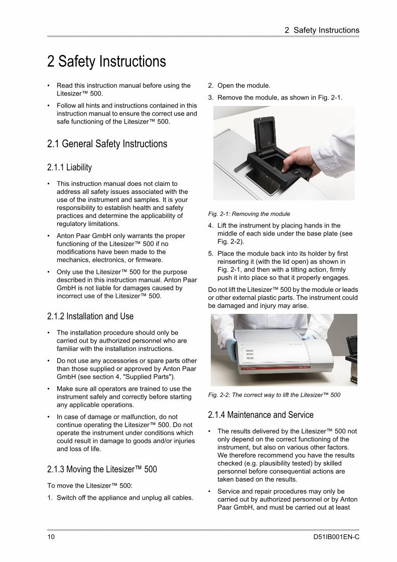
2. Open the module.
3. Remove the module, as shown in Fig. 2-1.
Fig. 2-1: Removing the module
4. Lift the instrument by placing hands in the middle of each side under the base plate (see Fig. 2-2).
5. Place the module back into its holder by first reinserting it (with the lid open) as shown in Fig. 2-1, and then with a tilting action, firmly push it into place so that it properly engages.
Do not lift the Litesizer™ 500 by the module or leads or other external plastic parts. The instrument could be damaged and injury may arise.
Fig. 2-2: The correct way to lift the Litesizer™ 500
2.1.4 Maintenance and Service
• The results delivered by the Litesizer™ 500 not only depend on the correct functioning of the instrument, but also on various other factors. We therefore recommend you have the results checked (e.g. plausibility tested) by skilled personnel before consequential actions are taken based on the results.
• Service and repair procedures may only be carried out by authorized personnel or by Anton Paar GmbH, and must be carried out at least
10 D51IB001EN-C

2 Safety Instructions
every 10 years to ensure product safety.
2.1.5 Disposal
• Concerning the disposal of the Litesizer™ 500, observe the legal requirements in your country.
2.1.6 Returns
• For repairs send the Litesizer™ 500 to your Anton Paar representative. Return the instrument and module together with the filled out "Maintenance/Error Report" and the "Standard Maintenance Contract". Find the applicable forms on the Anton Paar homepage (www.anton-paar.com).
2.1.6.1 Engaging the Transport Safety Lock
1. Switch off the instrument, remove the cuvette module, and unplug all cables.
2. Carefully lift the front of the instrument so that it
stands on its rear surface, as shown in Fig. 2-3.
Fig. 2-3: The Litesizer™ 500 standing on its rear surface
3. Insert the transport safety lock Torx key into one of the two small holes next to the module bay, as shown in Fig. 2-4.
Fig. 2-4: Insertion of Torx key
4. Gently turn the screw clockwise until it stops turning.
5. Repeat for the second hole.
The transport safety lock is now engaged.
NOTICE: Before packing the Litesizer™ 500 for transport, the transport safety lock must be engaged, as described below.
D51IB001EN-C 11

2 Safety Instructions
2.2 Safety Signs on the Litesizer™ 500
Fig. 2-5: Safety signs and laser aperture on the front surface of the module cavity
Fig. 2-6: Safety sign on the rear surface of the instrument
Fig. 2-7: "Hot surface" safety sign on the inside surface of the cuvette module lid (left) and on top of the thermal insulation cover (right)
CAUTION
Laser radiationSymbol position: Module cavity surface (Fig. 2-5).The Litesizer™ 500 is equipped with a laser of class 3B, which is integrated into the Litesizer™ 500, and therefore conforms to laser class 1 regulations. There is no exposure to laser radiation in the normal operation of this instrument. Follow your national safety regulations.
WARNING
Danger of laser radiationSymbol position: Module cavity surface (Fig. 2-5).Switch instrument off before handling any tools containing metal or other conducting materials in this area.
laseraperture
CAUTION
Risk of damage to instrumentSymbol position: Litesizer™ 500 rear surface (Fig. 2-6).Use dry air (ISO 8573.1, class 1.3.1) or nitrogen at 0.4 to 0.8 bar overpressure (1.4 to 1.8 bar total input).Use a 6 x 4 mm hose to connect the air/nitrogen. Failure to adhere to these specifications may result in damage to the instrument.
CAUTION
Hot surfaceSymbol position: On the inside surface of the cuvette module lid and on top of the thermal insulation cover (see Fig. 2-7).When making high-temperature measurements (above 45 ˚C), the cell area should be allowed to cool before removing the thermal insulation cover and cuvette.
safety sign
"hot surface"safety sign
12 D51IB001EN-C

2 Safety Instructions
2.3 Precautions for Using Flammable Samples or Cleaning Agents
• Place the unit in a well-ventilated area.
• Always use the purge port (see Fig. 12-2) with nitrogen as purge gas when measuring flammable samples (min. flow rate: 2 L/min).
• Do not measure any sample with a spontaneous ignition temperature of <279.87 ˚C.
• Flammable samples should be measured in quartz cuvettes at the lowest feasible measuring temperature.
• Fill the cuvette at a safe distance from the instrument in a well ventilated area, using only the minimum sample volume, and close the cuvette.
• Check the drain hole at the bottom of the cuvette module periodically using a pipe cleaner.
• Safely dispose of the sample as soon as possible after the measurement.
• If a flammable sample is spilled in or near the instrument:
- Switch off and unplug the instrument
- Remove cuvette module- If necessary let it cool down in a well-
ventilated place- Remove the vial from the cuvette- Remove all visible residue sample with a dry
cloth- Remove any remaining residue by blowing
with nitrogen or dry air- Do not reassemble the Litesizer™ 500 or
turn it on until all traces of sample residue have been removed.
- If in doubt, contact your Anton Paar service representative.
• Observe and adhere to your national safety regulations for handling samples and solvents (e.g. use of safety goggles, gloves, respiratory protection etc.).
• Only store the minimum required amount of sample, cleaning agents and other inflammable materials near the Litesizer™ 500.
• Connect the Litesizer™ 500 to the mains via a safety switch located at a safe distance from the instrument. In an emergency, turn off the power using this switch instead of the power switch on the Litesizer™ 500.
• Supply a fire extinguisher.
D51IB001EN-C 13

3 Litesizer™ 500 - An Overview
3 Litesizer™ 500 - An Overview
The Litesizer™ 500 is an instrument for characterizing particles in liquid dispersions. It determines particle size, zeta potential, and molecular mass by measuring dynamic (DLS), electrophoretic (ELS), and static light scattering (SLS). The Litesizer™ 500 should not be used in any other way than described in this manual.
cmPALS, a new ELS technology: Unique to the Litesizer™ 500 is cmPALS, a novel patented PALS technology (European Patent 2 735 870) that provides unprecedented accuracy in ELS measurements. Also, the incorporation of autoadjustment optics lends further stability to the Litesizer™ 500's optics, particularly in the long term. Despite these features, the Litesizer™ 500 is especially compact and lightweight.
Simple software: Particularly convenient is the Litesizer™ 500’s accompanying software program, Kalliope, which sets a new standard in user-friendliness. The user sees all important information on a single clear display, including input parameters, results, and final calculated values, as well as expert advice. Experiments can be performed in series with DLS and ELS, allowing the user to observe changes in particle properties while varying pH, time or temperature, for example.
Reporting: The Litesizer™ 500 enables fast and customizable analysis and reporting, and complies with the US FDA’s Regulation 21 CFR Part 11 concerning electronic records and signatures.
Transmittance: An extra capability of the Litesizer™ 500 includes continuous transmittance measurement. Transmittance measurements provide a fast indication of a sample's suitability for light-scattering measurements. In addition, this measurement allows the Litesizer™ 500 to select the best parameters for your sample (focus position, measuring angle, measurement duration).
3.1 Litesizer™ 500Measurement Specifications
Technology • Dynamic light scattering (DLS)
• Electrophoretic light scattering (ELS)
• Static light scattering (SLS)
• Transmittance
Light source Laser light of wavelength 658 nm from a single-frequency laser diode, providing 40 mW.
Laser warm-up time
• 6 min
Detection angles
• 15˚, 90˚, 175˚ (particle size)
• 15˚ (zeta potential)
• 90˚ (molecular mass)
Particle size range
• 0.3 nm – 10 m*
(particle size)
• 3.8 nm – 100 m(zeta potential)
• 980 Da – 20 MDa(molecular mass)
* under laboratory conditions
Minimum concentration
• 0.1 mg/mL (lysozyme)(particle size)
• 1 mg/mL (lysozyme)(zeta potential)
• 0.1 mg/mL (lysozyme)(molecular mass)
Temperature range
0–90 ˚C (32–194 ˚F)
Minimum volume
• 20 L(particle size)
• 350 L(zeta potential)
• 20 L(molecular mass)
14 D51IB001EN-C

3 Litesizer™ 500 - An Overview
3.2 Measurement Principles
3.2.1 Particle Size
Particle size is measured by dynamic light scattering (DLS). Particles suspended in a liquid are constantly undergoing random motion, and the speed of this motion depends on the size of the particles: smaller particles move faster than larger ones. In DLS, light is scattered by the sample, and the scattering is then detected and recorded many times. Comparison of those records with each other reveals how much the particles have moved in the time between each record (and therefore how fast they are moving). From this information, the average size of the particles can be calculated, as can the size distribution..
Fig. 3-1: Relative frequency vs. particle radius
3.2.2 Zeta Potential
Zeta potential is measured by electrophoretic light scattering (ELS), which measures the speed of the particles in the presence of an electric field. How fast the particles move depends on the surface charge, or zeta potential, of the particles. In general, the greater the magnitude of the zeta potential, the more stable the colloid.
Fig. 3-2: Relative frequency vs. zeta potential
3.2.3 Molecular Mass
Molecular mass is measured by static light scattering (SLS). In this case, the intensity of the scattered light is directly related to molecular mass. If the scattering intensity is measured at several different concentrations, then a Debye plot can be generated, the intercept of which provides the molecular mass.
Fig. 3-3: Debye plot (KC/R [mol/g] vs concentration)
3.2.4 Transmittance
Transmittance is measured by detecting the fraction of light that passes through the sample. The Litesizer™ 500 measures the transmittance continuously for every sample. The value is reported in real time and appears in the top right corner of the display any time the Litesizer™ 500 is in operation (see Fig. 3-4).
Fig. 3-4: Screen shot showing continuous transmittance reading
The transmittance of a sample can also be reported relative to the solvent, by first setting the solvent as the reference.
D51IB001EN-C 15

4 Supplied Parts
4 Supplied Parts The Litesizer™ 500 was tested and packed carefully before shipment. However, damage may occur during transport. Therefore:
1. Keep the packaging material (box, packing foam) for possible returns and further questions from the transport and insurance company.
2. Check the delivery for completeness by
comparing the supplied parts to those noted in the table, below.
3. If a part is missing, contact your Anton Paar representative.
4. If a part is damaged, contact the transport company and your Anton Paar representative.
Table 4-1: Supplied Parts
Symbol Pcs Article description Mat. no.
1 Litesizer™ 500 155761
1 Batch module: Two options:- BM10 (high-end batch module)- BM20 (batch module)
155764166281
1 Software package, Kalliope™ on USB stick. Three options:- Kalliope™ ProfessionalEnables access for three users- Kalliope™ Professional Single Addition. Enables access for one additional user- Kalliope™ Professional Unlimited. Enables access for an unlimited number of users
166116
170677
170678
1 Instruction manual 166212
1 Power cable (3x1.0 mm2, 10 A), according to country
- CEE
- UK
- USA
- China
- CH
- Thailand
- Brasil
52112
61865
52656
27011
93408
79730
130117
1 Power supply 12 V / 7.5 A 156217
1 USB cable 94228
1 Torx key T6 for transport safety lock 170679*
1 Starter kit (see table below) 155766
* Not available for separate sale
16 D51IB001EN-C

4 Supplied Parts
Table 4-2: Starter Kit
Symbol Pcs. Article description Mat. No.
1 Cuvette rack 163383
100 Disposable cuvettes (pack of 100)PS 10 x 10 x 45 mm
164435
100 Disposable cuvette lids (pack of 100) 163395
5 Omega cuvettes for zeta potential (box of 5; 20 male Luer plugs included)
155765
1 Thermal insulation cover 157666
1 Syringe filter – Anotop 10Anotop type 10 0.02µm syringe filter
163385
1 Syringe filter – Anotop 25Anotop type 25 0.02µm syringe filter
163388
D51IB001EN-C 17

5 Installation of the Litesizer™ 500
5 Installation of the Litesizer™ 500
5.1 Installation Requirements
The instrument should be placed on a stable, flat lab bench in a clean environment that is free from mechanical vibrations and excessive noise. Ensure that nothing is placed on top of the instrument.
To ensure temperature stability, place the Litesizer™ 500:
- away from heating- away from direct sunlight- away from open windows
Make sure that the power plug and the power switch are always easily accessible so that the instrument can be disconnected from the mains at any time.
A strong built-in cooling fan dissipates heat through the bottom and the back of the instrument (see Fig. 5-1). Ensure that the airflow is not blocked.
Read the Safety Instructions in Chapter 2.
Find all technical data in Appendix A - Technical Data.
PC requirements:
- Dual core system (or better)- 2 GB RAM (Windows 7 - 32 Bit) / 4 GB RAM
(Windows 7 - 64 Bit) (or better)- Windows 7 - Servicepack 1 (or better)- 5 GB HDD
5.2 Opening the Transport Safety Lock
1. Before switching the Litesizer™ 500 on or inserting the module or connecting any cables, carefully lift the front of the instrument so that it stands on its rear surface, as shown in Fig. 5-5.
Fig. 5-5: The Litesizer™ 500 on its rear surface
2. Insert the transport safety lock T6 Torx key into one of the two small holes next to the module bay, as shown in Fig. 5-6.
Fig. 5-6: Insertion of Torx key
3. Gently turn the screw anticlockwise until it stops turning.
4. Repeat for the second hole.
The transport safety lock is now open.
18 D51IB001EN-C

5 Installation of the Litesizer™ 500
5.3 Connecting the Instrument
Make sure the power switch is turned off. Make sure the transport safety lock is removed (see section 5.2). Connect the instrument to the computer via USB cable (see Fig. 5-1). Connect the AC/DC adapter to the instrument at the power socket. Make sure that mains voltage and frequency comply with the specified data (110/230 VAC, 50/60 Hz) of the AC/DC adapter. Connect the AC/DC Adapter to the mains voltage. Switch the instrument on at the main switch.
Fig. 5-1: Litesizer™ 500 rear surface
NOTE: The Litesizer™ 500 has a stand-by mode and a deep stand-by mode, which are activated after 15 min and 180 min of inactivity, respectively. For details, see section 6.2 below.
main switchpower socket
USB cable portcooling fan
D51IB001EN-C 19

6 How to Use the Litesizer™ 500
6 How to Use the Litesizer™ 500
6.1 Switching On
Switch the Litesizer™ 500 on at least ten minutes before you begin measurements. The power switch is at the back of the instrument.
Fig. 6-1: Litesizer™ 500 rear surface
6.2 Status and Stand-by Modes
When the Litesizer™ 500 is switched on, the POWER and STATUS indicator lights (Fig. 6-2) can each show two different colors, as listed in Table 6-1. After 15 min of inactivity, the instrument will go into stand-by mode, which means the laser will be switched off. After a further 180 min of inactivity, the instrument will go into deep stand-by mode, in which the temperature control is also switched off.
The device can be woken up from stand-by or deep
stand-by mode by pressing the button, opening the module cover or removing/inserting a module.
Fig. 6-2: The POWER and STATUS indicator lights
6.3 Starting the Software System, Kalliope
Install the software system, Kalliope. Start Kalliope by selecting "Programs > Kalliope" in the windows start menu or use the shortcut on the desktop.
6.4 Activating the Software License
When Kalliope is first started, you will be asked to enter a license code, as shown in Fig. 6-3. There are two ways to activate the software; either online or manually. For both, a valid license code is required.
Fig. 6-3: Entering the software license code
power switch
Table 6-1: POWER and STATUS indicator lights
POWER indicator
STATUS indicator
Meaning
blue green blinking
currently booting
green green successful boot, instrument in operation
blue red blinking
failure during boot
blue off stand-by (laser off)
blue "breathing"
off deep stand-by (temp. control off)
20 D51IB001EN-C

6 How to Use the Litesizer™ 500
6.4.1 Online Activation
For online activation, an internet connection is required.
1. In the "Online activation" tab, enter the valid license code provided with the delivery, as shown in Fig. 6-3.
2. Click Activate, then click Exit and restart the software.
6.4.2 Manual Activation
1. On the License Activation page, click the Man-ual activation tab at the top of the page (Fig. 6-4). Note the Machine code (Fig. 6-4, b) and the internet address (Fig. 6-4, a).
Fig. 6-4: Manual software license activation
2. On a PC with internet connection, go to the Anton Paar licensing webpage (https://aplicens-ing.azurewebsites.net/Activation/ActivateProj-ect/Kalliope; Fig. 4).
3.
4. Retrieving the activation code for manual license activation
5. Enter the valid license code provided with the delivery, and the machine code of the PC on which Kalliope is installed (Fig. 6-4, b), then click Activate. This will generate a valid activa-tion code.
6. Go back to the offline PC on which Kalliope is installed, and enter this activation code (Fig. 6-4, c).
7. Click Activate, then click Exit and restart the software. The display should now appear as in Fig. 6-5. If the instrument is connected to the computer and the software, a small green tick will appear in the top right corner.
Fig. 6-5: Kalliope start-up screen
NOTE RE SOFTWARE UPDATES: When uploading a new version of the software, the Litesizer™ 500 must be switched off.
D51IB001EN-C 21

6 How to Use the Litesizer™ 500
6.5 Checking the System
Clicking on the icon in the top left-hand corner opens the following menu (Fig. 6-6):
Fig. 6-6: Kalliope menu
6.6 Adjusting the Settings
Under the Kalliope menu, select "My settings" to open the menu shown in Fig. 6-6, which allows the user to select the preferred units, the data-handling mode, the particle-size dimensions that are reported (radius or diameter) and the preferred language.
Note that Kalliope needs to be restarted in order to apply new selections. Click again on the icon to close the window and return to the measurement window, above (Fig. 6-5).
Note regarding decimal points or commas: Kalliope will display either decimal commas or decimal points, according to your computer’s settings. This can only be changed in the user’s own computer settings, not within Kalliope itself.
22 D51IB001EN-C

6 How to Use the Litesizer™ 500
6.7 User Management
Under the Kalliope menu, select "Security" to open the menu shown in Fig. 6-7. To change the rights of existing users, or to add new users, check the "Enable user management" box. The Users list will then appear. New users can be added by clicking on the icon at the bottom of the screen, which brings up the list of names registered on the connected operating system. Users must be registered on the operating system (e.g. Windows 7) before they can be added to the instrument user list. Users’ rights can be changed by selecting "Basic", "Advanced" or "Administrator" from the drop-down menu, while users can be removed from the list by clicking on the icon.
Fig. 6-7: User management
6.8 Pharma Option (21 CFR Part 11)
In the "Security" menu shown in Fig. 6-7, check the second box under "Settings" to enable the pharma option. Note that "User Management" (section 6.7) must first be enabled before the pharma option can be enabled. Kalliope must be restarted to apply the new settings.
When using the pharma option, a workbook must be saved manually before a measurement can be started. Otherwise Autosave will not be enabled.
All documentation must be saved in a defined folder.
Once a measurement has started, the filename can no longer be changed. Furthermore, the measurement and its associated files cannot be deleted.
6.9 Performing a Measurement
On the start-up screen (Fig. 6-5), click on the icon to select a new measurement. The measurement options are displayed as follows (Fig. 6-8), with measurement modes on the left, and measurement series options on the right.
Fig. 6-8: Selection of measurement mode
Details for running each measurement mode can be found in the following chapters.
Note: Checking or unchecking the User Management box results in a change in the settings, and Kalliope must be restarted in order to apply the changes.
Note: A user must be logged in on the computer that is connected to the instrument in order to access the system and use the instrument.
D51IB001EN-C 23

7 Particle-Size Measurements
7 Particle-Size Measurements
7.1 Sample Preparation
Making a measurement with the Litesizer™ 500 is simple and straightforward. Nonetheless, the accuracy and precision of the results depend significantly on correct sample preparation for each type of measurement. Thus, it is important to follow the guidelines for preparing each type of sample, including choice of cuvette, choice of solvent, sample concentration, and filling of the cuvette.
7.1.1 Concentration
Particle-size measurements are significantly influenced by particle concentration. If the concentration is too low, then not enough light will be scattered to make a measurement. If the concentration is too high, then the light scattered by each particle may be further scattered by other particles (this effect is referred to as multiple scattering). A too-high concentration can also lead to distorted measurements because the particles can no longer undergo Brownian motion (free diffusion). Nonetheless, the ideal concentration varies for different particle sizes - see table below. For very small particles (<10 nm), there is no real maximum concentration.
For larger particles (>1 m), there is an additional effect to consider; i.e., that of number fluctuation. At low concentrations, the scattering intensity may still be high because larger particles scatter more effectively. But the number of particles in the scattering volume (the volume of overlap between the incident and detector beams) may be so small that number fluctuations significantly affect the results. Thus, the lower concentration limit for larger particles is such that there are at least 500 particles in the scattering volume (approximate scattering volumes are 106 µm3 for back scattering, 104 µm3 for side scattering, and 5 x 104 µm3 for forward scattering).
The following table shows the suitable range of particle concentration according to the expected particle size:
If the concentration is completely unknown, then in some cases, the visual appearance of a sample can be used as an indicator of concentration. Ideally, the sample should be prepared so that it is slightly cloudy, or turbid. Note, however, that samples of very small particles (<20 nm) will never become cloudy, even at high concentrations; whereas samples of very large particles will look turbid even at very low concentrations. Thus, in such cases, it is necessary to prepare and measure samples at several different concentrations in order to find the concentration range within which the results do not differ from each other more than the normal minor deviations. As a guide, the particle-size measurement should generate a mean detected light intensity of at least 20 kcounts/s. A further indicator is the filter optical density (attenuation level) used. For automatic measurements, a filter optical density of 0 also suggests that the sample concentration is low, although the results may still be meaningful if the count rate is still sufficiently high.
7.1.2 Solvent (or Dispersant) Selection
The solvent or dispersant should be distilled, deionized and/or filtered prior to use to ensure that it contains no unwanted particles, such as ions or dust, which may interfere with measurements.
All solvents or dispersants should be purified by filtration using a pore size of 10 or 20 nm. As an additional check, a particle-size measurement should be carried out on the solvent before mixing it with the material to ensure that it contains no unwanted particles.
Expected particle size
Minimum concentration
<10 nm 0.5 mg/mL
10 – 100 nm 0.1 mg/mL
100 nm – 1 m 0.01 mg/mL
>1 m 0.1 mg/mL
24 D51IB001EN-C

7 Particle-Size Measurements
The sample itself should not be filtered, because this may remove the particles to be measured. Samples should only be filtered if it is intended to remove large particles or agglomerates because they are not of interest or disturb the measurement.
7.1.3 Ultrasonication
Ultrasonication can be used to dissolve agglomerates or remove gas bubbles from the sample; however, ultrasonication should be used carefully, because it may initiate chemical reactions, thus distorting measurement results. Ideally, the effect of ultrasonication on the light-scattering properties of a sample should be checked by making measurements on a sample before and after ultrasonication.
7.2 Cuvettes
The standard cuvettes, both quartz and polystyrene, have inner dimensions of 10 mm x 10 mm x 45 mm. Ideally, the sample volume should be approximately 1 mL, but it must not be less than 0.85 mL or greater than 3 mL, as explained below.
Fig. 7-1: A standard cuvette showing the ideal sample volume.
The measurement is made 6.5 mm from the bottom of the cell, and the meniscus must be at least 2 mm above the measurement height (8.5 mm). For reliable measurements, the depth must be between 8.5 and 30 mm, and thus, the volume must be between 0.85 and 3 mL. If the sample volume is <0.85 mL, then the laser may be too close to the meniscus; if the sample volume is >3 mL, then the thermal equilibrium may not be stable.
7.2.1 Small-Volume Cuvette
The small-volume quartz cell is designed to be used when little sample is available. The maximum volume is 45 L, while the minimum that can be
used is 20 L.
Fig. 7-2: Small-volume cell showing the minimum sample volume (20 l)
7.2.2 Filling the Cuvettes
Disposable, powder-free latex gloves should be worn throughout all procedures; both to prevent skin contact with any samples or solvent, but also to protect the measurement cells and glassware from contaminants on/in the skin.
To fill a cuvette, place the tip of the pipette at the bottom of the cell so that it fills from the bottom up, thereby avoiding bubble formation. Check the sample through the windows for tiny bubbles, and tap the cell to dislodge any that have formed.
Place the lid firmly on the cuvette, and ensure that the outer surface is clean and dry before inserting it into the Litesizer™ 500.
7.2.3 Inserting the Cuvette
Open the chamber by pushing the OPEN button. Insert the cell firmly as far as it will go (see Fig. 7-3). Close the chamber.
Fig. 7-3: Inserting the cuvette
D51IB001EN-C 25

7 Particle-Size Measurements
7.3 Making a Measurement
On the start-up screen (Fig. 6-5), click on the icon to select a new measurement. Select . Input parameters can be entered on the left-hand side of the display, as follows (see Fig. 7-4). An explanation of the input parameters can be found in Table 7-2.
7.3.1 Input Parameters for Particle Size
Fig. 7-4: Input parameters for particle size
26 D51IB001EN-C

7 Particle-Size Measurements
Table 7-2: Explanation of input parameters for particle size
Title
Experiment name At the top is the name of the current measurement ("Untitled", in red). The name can be changed by clicking in any part of "Untitled". The back button will switch back to the overview display.
Comment Describe here the sample and/or conditions.
General
Measurement cell Disposable cell: suitable for all water-based samples (except proteins and particle sizes greater than 3 micrometers) for measurements up to 70 ˚C. Quartz cell: suitable for all non-water-based solvents/dispersants, for proteins and large-particle samples, and for high-temperature (up to 90 ˚C) measurementsSmall-volume cell: when a limited amount of sample is available.
Measurement angle Automatic: the optimum angle is automatically found for the sample, based on the transmittance, which is continuously measured. Back scatter (175˚): suitable for strongly scattering samples, including large particles, highly concentrated or turbid samples. Also suitable for weaker scatters and at low concentrationsSide scatter (90˚): suitable for weakly scattering samples, including small particles and transparent samples. It can be used for particles ranging from 0.3 nm up to 1 μm. Forward scatter (15˚): suitable for detection of large particles at low concentration; e.g., protein aggregates, infusion solutions
Target temperature Can be set from 0 to 90 ˚C. Note that for measurements above 70 ˚C, the quartz cell must be used.
TIP: Before making high- or low-temperature measurements, see Chapter 12, "Using the Litesizer™ 500 at High and Low Temperature".
Equilibration time For measurements close to ambient temperature, the equilibration time should be set at two minutes. The further the measuring temperature from ambient temperature, the longer the equilibration required (a common rule of thumb is to add one minute for every ˚C different from ambient temperature, based on a 1 mL sample).
Analysis model General: suitable if the sample is not well known, or if a single (broad) peak is expected.Narrow: Suitable if one or more narrow peaks is expected.
Cumulant model ISO 22412: default model.Advanced: suitable if any of the following features is visible in the correlation function:- elevated baseline (the correlation function decays to >1)- the correlation function is noisy- a second shoulder is visible (if you are sure that the second shoulder is an artifact or caused by dirt).
D51IB001EN-C 27

7 Particle-Size Measurements
Quality
Mode Automatic: time for each run (measurement time) will be 10 s, and the measurements will continue until the threshold number of counts has been accumulated (10 x 106) or until 60 runs have been made. Quick: the threshold number of counts is 3 x 10⁶, with maximum 30 runs. Manual: Number of runs and Time for each run must be manually selected.
Number of runs from 1 to 100
Time for each run[hh:mm:ss]
from 1 s to 30 min
Filter
Mode Automatic: the optical filter density will be automatically optimized based on the detected scattered intensity.Manual: the optical filter density must be manually selected.
Optical density from 0 to 6.5.
Focus
Mode Automatic: the focus position will be optimized automatically.Manual: the focus position must be manually selected.
Position From -4.5 to 3.5 mm, where 0 is the center of the cuvette. The optimal focus position varies not only for different samples, but also for the different scattering angles.
Material
Name Polystyrene latex, proteins, metal nanoparticles, etc.
The material must be selected from the user’s database. New materials can be entered on the database by the user by clicking on the icon. The material’s refractive index and absorption must also be entered into the database before they can be selected for a particle-size measurement. Once the material is selected, then the refractive index and absorption will be automatically filled.
Note: the temperature used in the measurement must be the same as that entered in the database.
Solvent
Name The solvent must be selected from the database.
Once the solvent is selected, then the refractive index and viscosity will be automatically filled. New solvents can be entered in the database by the user by clicking on the icon.
Note: the temperature used in the measurement must be the same as that entered in the database.
Table 7-2: Explanation of input parameters for particle size
28 D51IB001EN-C

7 Particle-Size Measurements
7.3.2 Starting a Measurement
Once the input parameters are complete, the icon in the bottom right-hand corner of the screen will be activated, and can be clicked to start the measurement.
Following temperature adjustment, equilibration and optical adjustment, the measurement will be displayed on the screen while it is running, as shown below, while the run number is displayed at the bottom of the screen. The Litesizer™ 500 will keep performing runs until a threshold number of counts has been accumulated (10 x 106 for automatic, or 3 x 10⁶ for Quick), or until the specified number of runs has been reached. Once the measurements are finished, all the measured and calculated values (see Table below for explanation) appear in the gray boxes to the right of the graphs, with the Mean hydrodynamic radius box appearing in green.
7.3.3 Measurement Output Screen
The measurement output screen retains a display of the input parameters on the left, a series of action icons at the top right, and the results (plots, automatic values and calculated values - see Fig. 7-5 to Fig. 7-8 and Table 7-4 to Table 7-6 below) on the main part of the screen at the right.
7.3.4 Action Icons
Fig. 7-5: Action icons (see top right-hand corner of screen)
Table 7-3: Explanation of the Action Icons
Exports current results to Excel file for further processing.
Recalculates the hydrodynamic radius. A new screen appears (see below), allow-ing the user to choose between the two possible cumulant models and the two analysis models. See appendix for fur-ther details.
Creates a copy of the input parameters of the current measurement. The name of the original measurement is retained, but with the prefix “New”.
Deletes current measurement, and switches back to starting display.
D51IB001EN-C 29

7 Particle-Size Measurements
7.3.5 Particle-Size Results - Intensity Trace and Related Values
Fig. 7-6: Particle size output: Intensity trace, filter optical density, focus position, angle used, mean intensity, and auto run criteria
Table 7-4: Explanation of Intensity Trace and Related Values
Filter optical density
Shows attenuation level used. For automatic measurements, a value of 0 suggests that the sample concentration is low, although the results may still be meaningful if the count rate is still sufficiently high.
Focus position Indicates the position of the optical focus used in the measurement.
Angle used Back scatter (175˚), forward scatter (15˚) or side scatter (90˚)
Intensity trace Plots intensity vs time. Appears as soon as the measurement has begun.
Mean intensity Displays mean detected light intensity in kcounts/s. If less than 20 kcounts/s, then increase the concentration.
Autorun criteria Displays the % of the threshold counts accumulated (10 x 106 counts for Automatic, 3 x 10⁶ for Quick). Nothing displayed for manual measurements.
30 D51IB001EN-C

7 Particle-Size Measurements
7.3.6 Particle-Size Results - Correlation Function and Hydrodynamic Radius
Further to the right on the screen is presented the correlation function, along with the mean
hydrodynamic radius, the polydispersity index, the g12 intercept and the baseline (see Fig. 7-7).
Fig. 7-7: Particle size output: mean hydrodynamic radius, polydispersity index, g12 intercept and baseline
Table 7-5: Explanation of Correlation Function and Related Values
Correlation function The measured autocorrelation function is plotted in white and the cumulant fit function in red.
Mean hydrodynamic radius
Shown in green for a successful measurement, or in red in case of an erroneous measurement.
Polydispersity index Indicates the breadth of the size distribution. A value of 10 % or less indicates that the sample is monodisperse, according to ISO 22412:2008(E) for 100 nm latex.
Intercept g12 The value of is g12 is g2 - 1 (where g2 is the correlation function intercept). For a good measurement, g12 will lie between 0.85 and 0.95. If g(1) > 1, there may be dust in the sample. Lower values indicate weak scattering or turbidity.
Baseline The baseline should ideally be 1.000. If the measured baseline deviates by more than 0.01, then according to ISO 22412:2008(E), the measurement is unreliable.
D51IB001EN-C 31

7 Particle-Size Measurements
7.3.7 Particle-Size Results - Size Distribution Function and Related Values
On the right-hand end of the screen is presented the particle radius distribution function, along with a list
of the peak values, and the number of processed runs.
Fig. 7-8: Particle size output: particle radius distribution function, peak values, and number of processed runs
Table 7-6: Explanation of Size Distribution Function and Related Values
Size distribution plot For the size distribution, the weighting model and parameter can be selected at the top of the graph field.
Peaks 1, 2 and 3 Up to three peaks from the size distribution plot will be listed here, indicating the most prevalent hydrodynamic radius of the particles.
Processed runs The number of runs measured. Note that only half of the measured runs are analyzed.
32 D51IB001EN-C

7 Particle-Size Measurements
7.4 Particle Size - Measurement Series
A series of particle-size measurements can be made by selecting New Measurement in Kalliope and then Particle size series, (see Fig. 7-9).
Fig. 7-9: Selecting a measurement series for particle size
7.4.1 Measurement Series Input Parameters
In addition to all of the input parameters, as described in section 7.3.1, the measurement series input parameters will appear at the right-hand end of the Input parameters screen (see Fig. 7-10).
Five parameters can be varied: temperature, concentration, pH, angle, or measurement focus (see Fig. 7-11). Alternatively, measurements can simply be repeated, as "repetition".
To set the number of measurements in the series, click on the icon until the required number of fields appears (see Fig. 7-12).
Once the input parameters are complete, click in the bottom right-hand corner of the screen.
For Temperature, Angle, Measurement focus and Repetition series, the measurements will continue automatically one after the other. For Concentration and pH measurement series, individual samples must be prepared for each measurement. The user will be asked to change the sample as each measurement is finished.
Fig. 7-10: Input parameters for a measurement series
Fig. 7-11: Series parameter selection
Fig. 7-12: Setting the number of measurements
NOTE: For a temperature series, ensure that sufficient equilibration time is allowed for each measurement. A general recommendation is to add 1 min for every ˚C difference between measurement temperatures, based on a 1 mL sample; e.g., for a series of three measurements at 20, 25, and 30 ˚C, at least 5 min equilibration time should be selected.
D51IB001EN-C 33
7 Particle-Size Measurements
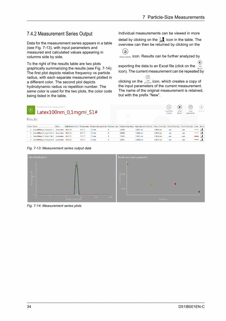
7.4.2 Measurement Series Output
Data for the measurement series appears in a table (see Fig. 7-13), with input parameters and measured and calculated values appearing in columns side by side.
To the right of the results table are two plots graphically summarizing the results (see Fig. 7-14): The first plot depicts relative frequency vs particle radius, with each separate measurement plotted in a different color. The second plot depicts hydrodynamic radius vs repetition number. The same color is used for the two plots, the color code being listed in the table.
Individual measurements can be viewed in more
detail by clicking on the icon in the table. The overview can then be returned by clicking on the
icon. Results can be further analyzed by
exporting the data to an Excel file (click on the
icon). The current measurement can be repeated by
clicking on the icon, which creates a copy of the input parameters of the current measurement. The name of the original measurement is retained, but with the prefix “New”.
Fig. 7-13: Measurement series output data
Fig. 7-14: Measurement series plots
34 D51IB001EN-C

7 Particle-Size Measurements
7.4.3 Comparison and Analysis of Data
Comparison of measurements from separate experiments is also possible through the Analyze function (although the measurements must be from the same workbook). The results of interest must first be open in Kalliope; results can be measured directly, or previously measured results can be accessed by clicking on the open workbook icon
. Once the results of interest are open in Kalliope, individual measurements can be selected for comparison and analysis by checking the white boxes in the left-hand column (see Fig. 7-15), which then contain a red tick. When at least two measurements have been selected, then the
Analyze icon will be activated. Clicking on the icon produces a graph of the relative frequency vs particle radius, with each separate measurement plotted in a different color, as well as a table of the data output, including measured and calculated values appearing in columns side by side (see Fig. 7-16). The weighting model used in the calculation can be selected by using the drop-down menu in the top right-hand corner of the graph.
As for measurement series (section 7.4.2, above), individual measurements can be viewed in more
detail by clicking on the icon in the table. The Analysis overview can then be returned by clicking
on the green back arrow icon at the left of the
screen (or on the icon).
7.4.4 Reporting
To present measurements or analyses as reports, see section 11, "Reporting".
Fig. 7-15: Selecting measurements to compare by using the Analyze function
Fig. 7-16: Output of the measurements selected for comparison by using the Analyze function
D51IB001EN-C 35

8 Zeta-Potential Measurements
8 Zeta-Potential Measurements
8.1 Sample Preparation
Zeta-potential measurements provide information about the stability of a colloidal dispersion. The zeta potential depends not only on the charge of the particles themselves, but also on the solvent in which the particles are dispersed. Therefore sample manipulation is only recommended for samples that cannot be measured in their original condition; for example, because the sample concentration is not within the required limits. Sample preparation may also be necessary for specific applications or special standardized measurement procedures, but every sample manipulation must be done carefully in order to not falsify the results.
8.1.1 Concentration
Zeta-potential measurements are not as sensitive to particle concentration as are particle-size measurements. Most importantly, the concentration must be high enough that sufficient light is scattered to provide meaningful measurements. As for particle size measurements, if a zeta potential measurement generates a mean detected light intensity of <20 kcounts/s, then the concentration should be increased if possible. Likewise, for automatic measurements, a filter optical density of 0 suggests that the sample concentration is low, although the results may still be meaningful if the count rate is still sufficiently high.
8.1.2 Diluting the Sample
Equilibrium dilution procedure: If the particle concentration is too high, the sample must be diluted, preferably by adding more of the solvent that is already in the sample, because the zeta potential will not be affected. This method is referred to as "equilibrium dilution procedure."
Solvent extraction/filtration: If no original solvent is available, it must be extracted from the original solution, either by sedimentation or centrifugation, but this only works well for large particles with sufficient density contrast. For small particles, dialysis is necessary with membranes that are not penetrable by the sample particles.
Solvent imitation: If the same solvent cannot be used, then a solvent should be sought whose properties match the original solvent as closely as
possible, in terms of viscosity, polarity, pH, electrolyte concentration.
8.2 Cuvettes
The Omega cuvettes for zeta potential are made from polycarbonate, and thus only aqueous samples may be used. The sample volume is 350 l, and the entire cell should be filled.
Disposable, powder-free latex gloves should be worn throughout all procedures; both to prevent skin contact with any samples or solvent, but also to protect the measurement cells and glassware from contaminants on/in the skin.
To fill the Omega cuvette, place the tip of the syringe snugly inside one of the sample ports (see Fig. 8-1, top). To stop bubbles forming, the filling direction should always be upwards. Thus, for the first half, the cell should be upside down. Gently inject the sample into the cuvette. Once the liquid reaches halfway (see Fig. 8-1, middle - see arrow), carefully turn the cell upright and continue to inject the sample until the cuvette is full (see Fig. 8-1, bottom).
Fig. 8-1: Filling the Omega cuvette: The cuvette should be held upside down until it is half full, so that the filling direction is always upwards.
36 D51IB001EN-C

8 Zeta-Potential Measurements
Ensure that both electrodes are covered by the sample. Check for tiny air bubbles and tap the cell to dislodge any that have formed. Insert the cuvette stoppers (see Fig. 8-2).
Fig. 8-2: Inserting the cuvette caps
8.2.1 Inserting the Cuvette
Ensure that the outer surface of the cuvette is clean and dry before inserting it into the Litesizer™ 500.
Open the chamber by pushing the OPEN button on top of the black module. Insert the cell firmly until it stops, with the electrodes and sample ports pointing to the sides (see Fig. 8-3). Close the chamber.
Fig. 8-3: Inserting the Omega cuvette
TIP: For advice on how to clean the Omega cuvettes, see Chapter 12, "Using the Litesizer™ 500 at High and Low Temperature".
8.3 Making a Measurement
On the start-up screen (Fig. 6-5), click on the icon to select a new measurement. Select . Input parameters can be entered on the left-hand side of the display, as follows (Fig. 8-4):
D51IB001EN-C 37

8 Zeta-Potential Measurements
8.3.1 Input Parameters for Zeta Potential
Fig. 8-4: Zeta potential input parameters
38 D51IB001EN-C

8 Zeta-Potential Measurements
Table 8-1: Explanation of Input Parameters for Zeta-potential Measurement
Title
Experiment name At the top is the name of the current measurement ("Untitled", in red). The name can be changed by clicking in any part of "Untitled". The back button will switch back to the overview display.
Comment Describe here the sample and/or conditions.
General
Measurement cell Omega cuvette: The Omega cuvette is made from polycarbonate; thus, only aqueous solvents may be used for these measurements.
Target temperature Measuring temperature must be manually entered, and must be set between 0 and 70 ˚C.
Equilibration time For measurements close to ambient temperature, the equilibration time should be set at two minutes. The further the measuring temperature from ambient temperature, the longer the equilibration required (a common rule of thumb is to add one minute for every ˚C different from ambient temperature, based on a 1 mL sample).
TIP: Before making high- or low-temperature measurements, see Chapter 12, "Using the Litesizer™ 500 at High and Low Temperature".
Approximation The Smoluchowski approximation is suitable for water-based samples.
Power adjustment
Adjustment mode Automatic: The voltage is increased in increments until the maximum voltage is reached, for which the maximum power is not exceeded. Manual: The voltage can be set from 0.1 to 200 V.
Voltage from 0.1 to 200 V
Quality
Run mode Automatic: the experiment will stop when the standard deviation reaches the threshold value.Manual: The number of runs can be set from 20 to 1000.
Number of runs from 20 to 1000
Solvent
Name The solvent must be selected from the database.
Note: Once the solvent is selected, then the Refractive index, viscosity and relative permittivity will be automatically filled. New solvents can be entered in the database by the user by clicking on the icon.
D51IB001EN-C 39

8 Zeta-Potential Measurements
8.3.2 Starting a Measurement
Once the input parameters are complete, the icon in the bottom right-hand corner of the screen will be activated, and can be clicked to start the measurement.
Following temperature adjustment, equilibration and optical adjustment, the measurement will be displayed on the screen while it is running, as shown below, while the run number is displayed at the bottom of the screen. The Litesizer™ 500 will keep performing runs until the standard deviation reaches the threshold value, or until the specified maximum number of runs has been reached. Once the measurements are finished, all the measured and calculated values (see Table 8-3 and Table 8-4 below for explanation) appear in the gray boxes to the right of the graphs, with the zeta potential box appearing in green.
8.4 Measurement Output Screen
The measurement output screen retains a display of the input parameters on the left, a series of action icons at the top right, and the results (plots, automatic values and calculated values - see
Fig. 8-5 to Fig. 8-7 and Table 8-2 to Table 8-4 below) on the main part of the screen at the right.
8.4.1 Action Icons
Fig. 8-5: Action icons (see top right-hand corner of screen)
Table 8-2: Explanation of Action Icons
Exports current results to Excel file for further processing.
Creates a copy of the input parameters of the current measurement. The name of the original measurement is retained, but with the prefix “New”.
Deletes current measurement, and switches back to starting display.
40 D51IB001EN-C

8 Zeta-Potential Measurements
8.4.2 Zeta-Potential Results - Intensity Trace and Related Values
Fig. 8-6: Zeta potential output I
8.4.3 Zeta-Potential Results - Phase Plot and Zeta-Potential Distribution
Fig. 8-7: Zeta potential output II
Table 8-3: Explanation of Intensity Trace and Related Values
Filter optical density Indicates the attenuation level used in the measurement. For automatic measurements, a filter optical density of 0 also suggests that the sample concentration is low, although the results may still be meaningful if the count rate is sufficiently high.
Mean intensity Displays the mean detected light intensity in kcounts/s. If the mean intensity is less than 20 kcounts/s, then increasing the concentration should give better results.
Adjusted voltage The voltage applied in the measurement.
Monitor trace Shows the interference between the modulated and unmodulated reference beams. A good measurement will show a stable signal with constant amplitude.
Detector trace Shows interference between scattered light from the sample and the modulated reference beam. An amplitude of at least 1000 is required to obtain meaningful results.
D51IB001EN-C 41

8 Zeta-Potential Measurements
Table 8-4: Explanation of Phase Plot, Zeta Potential Distribution and Related Values
Phase plot Plots the phase analysis light scattering (PALS), which shows the phase difference between the detector trace and the monitor trace in white. The blue line shows the fit of the PALS to the data.
Mean zeta potential The mean zeta potential is calculated from the phase analysis light scattering (PALS).
Electrophoretic mobility Calculated from the phase analysis light scattering (PALS).
Conductivity The conductivity should ideally be less than 1 mS/cm. The Litesizer™ 500 can measure zeta potential of samples with conductivities up to 200 mS/cm; however, such samples may be degraded or damaged by the voltage applied.
Standard deviation The standard deviation of the mean zeta potential.
Zeta potential distribution The Fourier transform of the detector trace is used to generate the zeta potential distribution as a function of frequency.
Distribution peak value The distribution peak is the maximum of the zeta potential distribution. The value should be similar to that generated from the PALS.
Processed runs Number of runs carried out in the measurement.
Auto run criteria "Reached" indicates that the threshold standard deviation was reached.
42 D51IB001EN-C

8 Zeta-Potential Measurements
8.5 Zeta Potential - Measurement Series
A series of zeta potential measurements can be made by selecting New Measurement in Kalliope and then selecting Zeta potential series (Fig. 8-8).
Fig. 8-8: Selecting a measurement series for zeta potential
8.5.1 Measurement Series Input Parameters
In addition to all of the input parameters, as described in section 8.3.1, the measurement series input parameters will appear at the right-hand end of the Input parameters screen (see Fig. 8-9).
The series can be based on variation of any one of four parameters: temperature, concentration, pH, (see Fig. 8-10); alternatively, the measurement can simply be repeated by selecting Repetition.
To set the number of measurements in the series, click on the icon until the required number of fields appears (see Fig. 8-11).
Once the input parameters are complete, click the icon in the bottom right-hand corner of the
screen to start the measurements.
For Temperature and Repetition series, the measurements will continue automatically one after the other. For Concentration and pH measurement series, individual samples must be prepared for each measurement. The user will be asked to change the sample as each measurement is finished.
Fig. 8-9: Input parameters for a measurement series
Fig. 8-10: Series parameter selection
Fig. 8-11: Setting the number of measurements
NOTE: For a temperature series, ensure that sufficient equilibration time is allowed for each measurement. A general recommendation is to add one minute for every ˚C difference between measurement temperatures, based on a 1 mL sample; e.g., for a series of three measurements at 20, 25, and 30 ˚C, at least 5 min equilibration time should be selected.
D51IB001EN-C 43

8 Zeta-Potential Measurements
8.5.2 Measurement Series Output
Data for the measurement series appears in a table (see Fig. 8-12), with input parameters and measured and calculated values appearing side by side. The order of the values can be changed by clicking on the column heading and dragging it to the desired position.
To the right of the results table are two plots graphically summarizing the results (see Fig. 8-13): The first plot depicts relative frequency vs zeta potential, with each separate measurement plotted in a different color. The second plot depicts mean zeta potential vs repetition number. The same color is used for the two plots, the color code being listed in the table.
Individual measurements can be viewed in more
detail by clicking on the icon in the table. The overview can then be returned by clicking on the
icon. Results can be further analyzed by
exporting the data to an Excel file (click on the
icon). The current measurement can be repeated by
clicking on the icon, which creates a copy of the input parameters of the current measurement. The name of the original measurement is retained, but with the prefix “New”.
Fig. 8-12: Measurement series output data
Fig. 8-13: Measurement series plots
44 D51IB001EN-C

8 Zeta-Potential Measurements
8.5.3 Comparison and Analysis of Data
Comparison of measurements from separate experiments is also possible through the Analyze function. The results of interest must first be open in Kalliope. Results can be measured directly; or previously measured results can be accessed by
clicking on the open workbook icon . Once the results of interest are open in Kalliope, individual measurements can be selected for comparison and analysis by checking the white boxes in the left-hand column (see Fig. 8-14), which then contain a red tick. When at least two measurements have
been selected, then the Analyze icon will be activated. Clicking on the icon plots a graph of the relative frequency vs zeta potential, with each separate measurement plotted in a different color, as well as a table of the data output, including measured and calculated values (see Fig. 8-15).
As for measurement series (Chapter 8.5.3, "Comparison and Analysis of Data", above), individual measurements can be viewed in more
detail by clicking on the icon in the table. The Analysis overview can then be returned by clicking
on the green back arrow icon at the left of the
screen (or by clicking on the icon).
Fig. 8-14: Selecting measurements to compare by using the Analyze function
8.5.4 Reporting
To present measurements or analyses as reports, see section 11, "Reporting".
Fig. 8-15: Output of the measurements selected for comparison by using the Analyze function
D51IB001EN-C 45

9 Molecular-Mass Measurements
9 Molecular-Mass Measurements
9.1 Sample Preparation
For molecular mass measurements, the sample preparation is similar to that for particle size measurements, in that mass measurements are particularly sensitive to dust or other contaminants in the solvent. Thus, solvents should be filtered several times before making up samples. All glassware and equipment used for sample preparation should be scrupulously clean and free of dust and scratches.
It is advisable to use at least three samples of different concentrations in order to generate the Debye plot. Furthermore, a sample of the solvent, and of the reference must also be made up fresh. The solvent sample must include all solutes (such as buffer or salt) that are contained in the sample other than the particles to be measured.
As for particle-size and zeta-potential measurements, if a molecular-mass measurement generates a mean detected light intensity of <20 kcounts/s, then the concentration should be increased.
9.2 Cuvettes
The standard cells for molecular mass measurements are quartz, with inner dimensions 10 mm x 10 mm x 45 mm. Ideally, the sample volume should be approximately 1 mL.
Fig. 9-1: A standard cuvette showing the ideal sample volume.
The measurement is made 6.5 mm from the bottom of the cell, and the meniscus must be at least 2 mm above the measurement height (8.5 mm). For reliable measurements, the depth must be between 8.5 and 30 mm, and thus, the volume must be between 0.85 and 3 mL.
9.2.1 Small-Volume Cuvette
The small-volume quartz cell is designed to be used when little sample is available. The maximum volume is 45 l, while the minimum that can be used is 20 l.
Fig. 9-2: Small-volume cell showing the minimum sample volume (20 l)
9.2.2 Filling the Cuvettes
Disposable, powder-free latex gloves should be worn throughout all procedures; both to prevent skin contact with any samples or solvent, but also to protect the measurement cells and glassware from contaminants on/in the skin.
To fill a cuvette, place the tip of the pipette at the bottom of the cell so that it fills from the bottom up, thereby avoiding bubble formation. Check the sample through the windows for tiny bubbles, and tap the cell to dislodge any that have formed.
Place the lid firmly on the cuvette, and ensure that the outer surface of the cuvette is clean and dry before inserting it into the Litesizer™ 500.
9.2.3 Inserting the Cuvette
Open the chamber by pushing the OPEN button. Insert the cell firmly until it stops (see Fig. 9-3). Close the chamber.
Fig. 9-3: Inserting the cuvette
46 D51IB001EN-C

9 Molecular-Mass Measurements
9.3 Making a Measurement
On the start-up screen (Fig. 6-5), click on the icon to select a new measurement. Select . Input parameters can be entered on the left-hand side of the display, as described in Fig. 9-4 and Table 9-1, below.
9.3.1 Input Parameters for Molecular Mass
Fig. 9-4: Molecular-mass input parameters
D51IB001EN-C 47

9 Molecular-Mass Measurements
Table 9-1: Explanation of Input Parameters for Molecular Mass
Title
Experiment name At the top is the name of the measurement. Click in any part of "Untitled" to change the name. The back button switches back to the overview display.
Comment Describe here the sample and/or conditions.
General
Measurement cell Quartz: the only cell that can be used for molecular mass measurements
Target temperature Measuring temperature must be set between 0 and 90 ˚C (entered manually)
TIP: Before making high- or low-temperature measurements, see Chapter 12, "Using the Litesizer™ 500 at High and Low Temperature".
Equilibration time For measurements close to ambient temperature, the equilibration time should be set at two minutes. The further the measuring temperature from ambient temperature, the longer the equilibration required (add one minute for every ˚C different from ambient temperature, based on a 1 mL sample).
dn/dc This is the refractive index increment. It represents the change in refractive index as a function of the change in concentration.
Quality
Mode automatic or manual
Number of runs from 1 to 100
Time for each run must be set between 1 s and 30 min
Solvent
Name Select a solvent from the database.
Note: Once the solvent is selected, then the Refractive index will be automatically filled. New solvents can be entered in the database by the user by clicking on the icon.
Reference
Name Toluene is generally used as the reference. Once the reference is selected, the refractive index and Rayleigh ratio will be automatically imported from the solvent database. New references can be entered in the solvent database by clicking on the icon.
Shape correction
Shape A shape correction should be selected if the particles do not scatter isotropically. Spherical, spiral, cylindrical, or "no correction" can be selected.
Hydrodynamic radius The hydrodynamic radius must be inserted if known, or it must first be measured by performing a particle-size measurement.
Concentrations
At least three concentrations are required to make a measurement. Additional concentrations can be entered by clicking on the icon, while a concentration can be deleted by clicking on the icon. Con-centrations can be selected between 0.001 and 500 mg/mL.
48 D51IB001EN-C

9 Molecular-Mass Measurements
Note: regardless of input order, the Litesizer™ 500 will measure in order of concentration, starting from the most concentrated sample.
Table 9-1: Explanation of Input Parameters for Molecular Mass
D51IB001EN-C 49

9 Molecular-Mass Measurements
9.3.2 Starting a Measurement
Once the input parameters are complete, the icon in the bottom right-hand corner of the screen will be activated, and can be clicked to start the measurement. You will then be asked to insert each sample in succession, starting from the most concentrated sample down to the least concentrated sample (regardless of which order they are entered in the Input), followed by the solvent sample, and finally the reference. Sample measurement starts after the optics adjustment and sample equilibration. Once sample measurement begins, the results will appear on the right-hand side of the screen. Once the measurements are finished, all the measured and calculated values can be seen in the gray boxes to the right of the graphs.
9.4 Measurement Output Screen
The measurement output screen retains a display of the input parameters on the left, a series of action icons at the top right, and the results (plots, automatic values and calculated values—see
Fig. 9-5 to Fig. 9-7 and Table 9-2 to Table 9-4 below) on the main part of the screen at the right.
9.4.1 Action Icons
Fig. 9-5: Action icons (see top right-hand corner of screen)
Table 9-2: Explanation of Action Icons
Exports current results to Excel file for further processing.
Creates a copy of the input parameters of the current measurement. The name of the original measurement is retained, but with the prefix “New”.
Deletes current measurement, and switches back to starting display.
50 D51IB001EN-C

9 Molecular-Mass Measurements
9.4.2 Molecular-Mass Results - Intensity Trace and Related Values
Fig. 9-6: Molecular mass output I
Table 9-3: Explanation of Intensity Trace and Related Values
Intensity trace The intensity trace displays the current measurement as soon as it begins.
Mean intensity Displays the mean detected light intensity in kcounts/s. If the mean intensity is less than 20 kcounts/s, then increasing the concentration should give better results.
Filter optical density
Indicates the attenuation level used in the measurement. For automatic measure-ments, a filter optical density of 0 also suggests that the sample concentration is low, although the results may still be meaningful if the count rate is still sufficiently high.
Focus position Indicates the position of the optical focus used in the measurement.
D51IB001EN-C 51

9 Molecular-Mass Measurements
9.4.3 Molecular-Mass Results - Debye Plot, Molecular Mass and 2nd Virial Coefficient
Fig. 9-7: Molecular mass output II
Table 9-4: Explanation of Debye Plot, Molecular Mass and 2nd Virial Coefficient
Debye plot The Debye plot relates the intensity of the scattered light (KC/R) to the particle concentration.
Molecular mass Calculated as the inverse of the Y-intercept of the Debye plot.
2nd virial coefficient
Calculated from the slope of the Debye plot. Reflects the interaction between particles and solvent, and between the particles. A positive gradient indicates that the particle–solvent interactions are stronger than the particle–particle interactions, so the dispersion or solution is stable. Vice versa, a negative gradient indicates that the particle–particle interactions are stronger than the particle–solvent interactions, so the particles will tend to aggregate.
Intensity vs concentration
The mean intensity from each sample is plotted vs concentration, which should give a linear relationship. Deviations from linearity may indicate that one or more of the measurements is erroneous; for example, the sample may contain dust or other contaminants.
52 D51IB001EN-C

10 Transmittance Measurements
10 Transmittance Measurements
10.1 Sample Preparation
There are no real restrictions on the type of samples that can undergo transmittance measurements. For aqueous samples, the disposable polystyrene cuvettes can be used. For all other solvents, the quartz cells should be used.
10.1.1 Reference Sample
Along with the sample to be measured, a sample of the neat solvent should be prepared with the same sample volume, and in the same type of cuvette. The solvent sample can then be used as the reference.
10.2 Cuvettes
The standard cells, both quartz and polystyrene, have inner dimensions of 10 mm x 10 mm x 45 mm. Ideally, the sample volume should be approximately 1 mL.
Fig. 10-1: A standard cuvette showing the ideal sample volume.
The measurement is made 6.5 mm from the bottom
of the cell, and the meniscus must be at least two mm above the measurement height (8.5 mm). For reliable measurements, the depth must be between 8.5 and 30 mm, and thus, the volume must be between 0.85 and 3 mL.
10.2.1 Filling the Cuvettes
Disposable, powder-free latex gloves should be worn throughout all procedures to protect the cuvettes and glassware from natural oils and contaminants on/in the skin, but also to prevent skin contact with any samples or solvent.
Hold the cuvette at an angle and allow the sample to run slowly down the internal corner. Such a technique should stop bubbles forming. Place the lid firmly on the cuvette, and ensure that the outer surface of the cuvette is clean and dry before inserting it into the Litesizer™ 500.
10.2.2 Inserting the Cuvette
Open the chamber by pushing the OPEN button. Insert the cell firmly until it stops (see Fig. 9-3). Close the chamber.
Fig. 10-2: Inserting the cuvette
D51IB001EN-C 53

10 Transmittance Measurements
10.3 Making a Measurement
On the start-up screen (Fig. 6-5), click on the icon to select a new measurement. Select
. Input parameters can be entered on the left-hand side of the display, as described in Fig. 10-3 and Table 10-1, below:
10.3.1 Input Parameters for Transmittance
Fig. 10-3: Input parameters for transmittance
Table 10-1: Input Parameters
Title
Experiment name At the top is the name of the current measurement ("Untitled", in red). The name
can be changed by clicking in any part of "Untitled". The back button will switch back to the overview display.
Comment Describe here the sample and/or conditions.
General
Target temperature Measuring temperature must be manually entered, and must be set between 0 and 90 ˚C (or 273 and 363 K).Note: for measurements above 70 ˚C, the quartz cell must be used.
TIP: Before making high- or low-temperature measurements, see Chapter 12, "Using the Litesizer™ 500 at High and Low Temperature".
Equilibration time For measurements close to ambient temperature, the equilibration time should be set at 2 min. The further the measuring temperature from ambient tempera-ture, the longer the equilibration required (a common rule of thumb is to add 1 min for every ˚C different from ambient temperature, for a 1 mL sample).
Quality
Time for each run must be set between 1 s and 30 min. The recommended initial Time for each run is 10 s.
54 D51IB001EN-C

10 Transmittance Measurements
10.3.2 Starting a Measurement
Once the input parameters are complete, the icon in the bottom right-hand corner of the screen will be activated, and can be clicked to start the measurement. Sample measurement starts after the optics adjustment and sample equilibration. Once sample measurement begins, the results will appear on the right-hand side of the screen. Once the measurement is finished, the results can be seen in the gray boxes to the right of the graphs.
10.4 Measurement Output Screen
The measurement output screen retains a display of the input parameters on the left, a series of action icons at the top right, and the results (plots, automatic values and calculated values—see Fig. 10-4 to Fig. 10-5 and Table 10-2 to Table 10-3 below) on the main part of the screen at the right.
10.4.1 Action Icons
Fig. 10-4: Action icons (see top right hand corner of screen)
Note: To set the reference, a sample of the neat solvent or dispersant should be used. Once the trans-
mittance is measured, click on the icon. Then use the back button to start a new measurement with the new reference. If no reference measurement is made, then the transmittance of the empty chamber (with no cuvette) will be taken as the reference value.
Table 10-1: Input Parameters
Table 10-2: Explanation of Action Icons
Sets the transmittance of the current sample as the reference.
Exports current results to Excel file for further processing.
Creates a copy of the input parameters of the current measurement. The name of the original measurement is retained, but with the prefix “New”.
Deletes current measurement, and switches back to starting display.
D51IB001EN-C 55

10 Transmittance Measurements
10.4.2 Transmittance Results
Fig. 10-5: Transmittance output
Table 10-3: Explanation of Transmittance Results
Mean transmittance Colored green. Transmittance relative to reference power, which is set to 100 %.
Mean power Mean transmitted power of the current measurement, in watts.
Reference power Mean transmitted power of the reference measurement, in watts. If no extra refer-ence measurement is made, then the reference will be taken as the power trans-mitted through an empty chamber.
Note: To find out whether a sample changes over time (e.g. through sedimentation or aggregation), then it is advisable to repeat the transmittance measurement at certain time intervals
56 D51IB001EN-C

11 Reporting
11 Reporting
11.1 Reports of Individual Measurements
To present an individual measurement as a reports, the measurement must first be selected from an open workbook by checking the white box in the left-hand column (see Fig. 11-1). The box then contains
a red tick and the report icon in the bottom
right-hand corner is activated. Clicking on the icon allows you to select a report template (which can be customized as described in ), which then produces a comprehensive summary of the data output, including measured and calculated values, in a convenient report format. Once created, the report can be forwarded for Review and/or Approval, either
electronically by clicking on the Sign icon , or in hard copy by collecting the appropriate signatures at the end of the report.
11.2 Reports of Measurement Series
Measurement series can also be presented as reports. This can be done by either selecting a measurement series, in the same way as described above for reports of individual measurements, or from within an analysis. Once an analysis is open in
Kalliope, the report icon can be found in the top-right corner of the page.
Fig. 11-1: Selecting a measurement for creating a report
11.3 Customizing Reports
Customized reports can be produced by opening the Kalliope menu and selecting Reporting. The simplest way to proceed is to select the Standard report under the appropriate mode (see Fig. 11-2),
then click on the copy icon in the top right-hand corner.
Fig. 11-2: Customizing a report
D51IB001EN-C 57

11 Reporting
This creates a "Copy of Standard report". Clicking
on the edit icon (next to the Copy icon) opens the report template designer (see Fig. 11-3). The report can now be renamed, while items can be
added or removed by clicking on the the icon or
the delete icon , respectively. The template can be saved and closed by clicking on the close icon
in the top right-hand corner. To access the
template, click on the report icon , as described
in section 11.1 or section 11.2, above.
Fig. 11-3: Report template designer
58 D51IB001EN-C
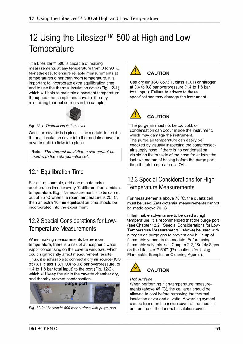
12 Using the Litesizer™ 500 at High and Low Temperature
12 Using the Litesizer™ 500 at High and Low TemperatureThe Litesizer™ 500 is capable of making measurements at any temperature from 0 to 90 ˚C. Nonetheless, to ensure reliable measurements at temperatures other than room temperature, it is important to incorporate extra equilibration time, and to use the thermal insulation cover (Fig. 12-1), which will help to maintain a constant temperature throughout the sample and cuvette, thereby minimizing thermal currents in the sample.
Fig. 12-1: Thermal insulation cover
Once the cuvette is in place in the module, insert the thermal insulation cover into the module above the cuvette until it clicks into place.
12.1 Equilibration Time
For a 1 mL sample, add one minute extra equilibration time for every ̊ C different from ambient temperature. E.g., if a measurement is to be carried out at 35 ˚C when the room temperature is 25 ˚C, then an extra 10 min equilibration time should be incorporated into the experiment.
12.2 Special Considerations for Low-Temperature Measurements
When making measurements below room temperature, there is a risk of atmospheric water vapor condensing on the cuvette windows, which could significantly affect measurement results. Thus, it is advisable to connect a dry air source (ISO 8573.1, class 1.3.1, 0.4 to 0.8 bar overpressure, or 1.4 to 1.8 bar total input) to the port (Fig. 12-2), which will keep the air in the cuvette chamber dry, and thereby prevent condensation.
Fig. 12-2: Litesizer™ 500 rear surface with purge port
12.3 Special Considerations for High-Temperature Measurements
For measurements above 70 ˚C, the quartz cell must be used. Zeta-potential measurements cannot be made above 70 ˚C.
If flammable solvents are to be used at high temperature, it is recommended that the purge port (see Chapter 12.2, "Special Considerations for Low-Temperature Measurements", above) be used with nitrogen as purge gas to prevent any build up of flammable vapors in the module. Before using flammable solvents, see Chapter 2.2, "Safety Signs on the Litesizer™ 500" (Precautions for Using Flammable Samples or Cleaning Agents).
Note: The thermal insulation cover cannot be used with the zeta-potential cell.
purge port
CAUTION
Use dry air (ISO 8573.1, class 1.3.1) or nitrogen at 0.4 to 0.8 bar overpressure (1.4 to 1.8 bar total input). Failure to adhere to these specifications may damage the instrument.
CAUTION
The purge air must not be too cold, or condensation can occur inside the instrument, which may damage the instrument.The purge air temperature can easily be checked by visually inspecting the compressed-air supply hose; if there is no condensation visible on the outside of the hose for at least the last two meters of hosing before the purge port, then the air temperature is OK.
CAUTION
Hot surfaceWhen performing high-temperature measure-ments (above 45 ˚C), the cell area should be allowed to cool before removing the thermal insulation cover and cuvette. A warning symbol can be found on the inside cover of the module and on top of the thermal insulation cover.
D51IB001EN-C 59

13 Cleaning the Litesizer™ 500 and Cuvettes
13 Cleaning the Litesizer™ 500 and Cuvettes
13.1 Cleaning the Instrument
To clean the instrument housing, use warm water with a mild cleaning agent (pH<10), or ethanol.
It is not advisable to apply cleaning agents or any other liquids inside the module of the Litesizer™ 500.
13.2 Cleaning the Cuvettes
13.2.1 Disposable Cuvettes
Do not clean and reuse the disposable cuvettes.
They are likely to give erroneous results on subsequent uses.
13.2.2 Quartz Cuvettes
1. Rinse with the solvent that was used for the measurement.
2. Rinse with purified water.
3. Rinse with acetone or ethanol and dry in a warm oven (50–60 ˚C).
4. If any residue remains, a pipe cleaner may be used to dislodge the residue before repeating steps 2 and 3.
13.2.3 Omega Cuvettes
1. Flush three times with purified water by using a syringe with the tip inserted into one of the sample ports (see Fig. 8-1, top)
2. Flush with dry air.
NOTICEIn case of a spillage inside the cuvette module, use a lens cleaning cloth or equivalent material that does not leave fibers behind. Wet the lens cloth or lens tissue with water and gently wipe out the module. Wet a further cloth with ethanol or acetone to remove any residual water, as well as any water-insoluble residue.
NOTICENever use:
• organic solvents (e.g. toluene, hexane, acetone, chloroform)
• strong acids or bases (e.g. nitric acid, sulfuric acid, hydrochloric acid, caustic soda)
• strong mechanical action (steel brush)
NOTICENever use organic solvents (e.g. toluene, hexane, acetone, chloroform) to clean the Omega cuvettes.Never use ultrasound to clean the Omega cuvettes.
60 D51IB001EN-C

14 Validation Protocol
14 Validation ProtocolThis procedure is for validating the performance of the Litesizer™ 500. The validation should be carried out every six months or when the device is moved to a different location.
14.1 Preparation of Latex Samples for Particle-size Measurements(see Methods in Kalliope)
14.1.1 Sample for Validation A: Concentrated 220 nm Latex for Back-Angle Measurement
1. A laminar-flow cabinet should be used for these
steps where possible.
2. Discard the first drop of latex from the bottle and add 1 drop of standard to a disposable cuvette.
3. Add 1 mL of 0.9 % NaCl solution.
4. Place a cap on the cuvette and mix for a few seconds prior to measurement.
14.1.2 Sample for Validation B: Dilute 220 nm Latex for Side-Angle Measurement
1. A laminar-flow cabinet should be used for these steps where possible.
2. Using a syringe, transfer 100 L of validation sample A into a disposable cuvette.
3. Add 2 mL of 0.9 % NaCl solution.
4. Place a cap on the cuvette and mix for a few seconds.
5. Transfer 1 mL to a new disposable cuvette, place the cap on, and measure it.
14.1.3 Sample for Validation C: Preparation of Ludox TM40 for Zeta Potential
1. Rinse the Omega cuvette with water, as described in section 13.2.3.
2. Dilute the stock solution (40 % w/v) to a final concentration of 4 % (w/v).
3. Fill the cell with the stock solution (350 L).
4. Ensure that there are no bubbles in the cell and close it with the stoppers.
Table 14-1: Equipment Required for Validation Protocol
Latex 220 nm standard (Mat. No. 165156)*
* the stated size may change according to the supplier batch
Ludox TM-40 (Mat. No. 165157)
NaCl solution (0.9 %)
Toluene, anhydrous 99.7 %
Deionized water
Disposable cuvettes (Mat. No. 164435)
1 Glass cuvette
1 Omega cuvette for zeta potential (Mat. No. 155765)
Anotop type 25 0.02 µm syringe filter (Mat. No. 163388)
D51IB001EN-C 61
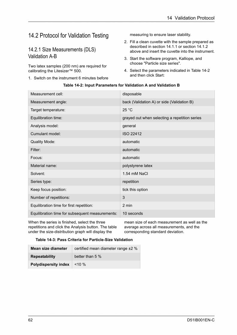
14 Validation Protocol
14.2 Protocol for Validation Testing
14.2.1 Size Measurements (DLS)Validation A-B
Two latex samples (200 nm) are required for calibrating the Litesizer™ 500.
1. Switch on the instrument 6 minutes before
measuring to ensure laser stability.
2. Fill a clean cuvette with the sample prepared as described in section 14.1.1 or section 14.1.2 above and insert the cuvette into the instrument.
3. Start the software program, Kalliope, and choose "Particle size series".
4. Select the parameters indicated in Table 14-2 and then click Start:
When the series is finished, select the three repetitions and click the Analysis button. The table under the size-distribution graph will display the
mean size of each measurement as well as the average across all measurements, and the corresponding standard deviation.
Table 14-2: Input Parameters for Validation A and Validation B
Measurement cell: disposable
Measurement angle: back (Validation A) or side (Validation B)
Target temperature: 25 °C
Equilibration time: grayed out when selecting a repetition series
Analysis model: general
Cumulant model: ISO 22412
Quality Mode: automatic
Filter: automatic
Focus: automatic
Material name: polystyrene latex
Solvent: 1.54 mM NaCl
Series type: repetition
Keep focus position: tick this option
Number of repetitions: 3
Equilibration time for first repetition: 2 min
Equilibration time for subsequent measurements: 10 seconds
Table 14-3: Pass Criteria for Particle-Size Validation
Mean size diameter certified mean diameter range ±2 %
Repeatability better than 5 %
Polydispersity index <10 %
62 D51IB001EN-C

14 Validation Protocol
14.2.2 Zeta-Potential Measurements (ELS)Validation C
1. Switch on the instrument 6 minutes before measuring to ensure laser stability.
2. Fill a clean cuvette with the sample prepared as described in section 14.1.3 and insert the
cuvette into the instrument.
3. Start the software program, Kalliope, and choose "zeta potential series".
4. Choose the test parameters as indicated in Table 14-4 below
5. Click Start
When the series has finished, select the three repetitions and click on the Analysis button. The table under the zeta-potential distribution graph will display the mean zeta potential of every measurement as well as the average across all measurements and the corresponding standard deviation.
Table 14-4: Input Parameters for Validation C
Measurement cell Omega cuvette
Target temperature 25 °C
Equilibration time grayed out when selecting a repetition series
Adjustment mode automatic
Run mode Automatic
Solvent Water
Number of repetitions 3
Equilibration time for first repetition 2 min
Equilibration time for subsequent measurements 10 seconds
Table 14-5: Pass Criterion for Zeta-Potential Validation
Mean zeta potential -38 mV ± 10 %
D51IB001EN-C 63

14 Validation Protocol
14.2.3 Molecular-Mass Measurement (SLS)Validation D
1. Switch on the instrument 6 minutes before measuring to ensure laser stability.
2. Prepare a sample of toluene by filtering through a 0.02 μm membrane filter into a quartz cuvette.
3. Start the software program, Kalliope, and choose "molecular mass".
4. Choose the test parameters as indicated in Table 14-6 below.
5. Click Start.
Leave the cell in the instrument until the measurement is finished. When indicated by the Litesizer, open the module, remove the cell and insert the next sample. Close the module and click ok.
Table 14-6: Input Parameters for Validation D
Measurement cell Quartz
Target temperature 25 °C
Equilibration time 3 min
dn/dc 1 mL/g
Quality mode manual
Number of runs 3
Measurement time 10 seconds
Solvent toluene
Reference toluene
Shape correction no correction
Concentrations 1 mg/mL; 2 mg/mL; 3 mg/mL
Table 14-7: Pass Criterion for Molecular-Mass Validation
Molecular mass <10 Da*
* 0 is a valid number
64 D51IB001EN-C

Appendix A: Technical Data
Appendix A: Technical DataPhysical Specifications
Dimensions (w x d x h) 460 mm x 485 mm x 135 mm
Weight 18 kg
Housing Material
Front, top & side cover Noryl™ FN215X: polyphenylene ether/polystyrene
Back, bottom stainless steel
Module PPS GF 40: polyphenylene sulfide + glass fibers
Omega cuvettes Cuvette body: polycarbonate/Electrodes: goldCaps: poly(ethene-co-tetrafluoroethene)
Power
Power supply at instrument 12 V via external adapter
Power supply for AC adapter 230 VAC, 50/60 Hz
Power consumption 50 W
Environmental Conditions
Ambient temperature +10 to +35 °C
Ambient humidity up to 90 % non-condensing
Airborne noise emission < 70 dB
Degree of pollution 2
Air/Gas Supply
Quality clean, dry and oil-free (ISO 8573.1, class 1.3.1)
Pressure 0.4 to 0.8 bar overpressure, or 1.4 to 1.8 bar total input
Wetted Parts
The following materials are in contact, or may come into contact, with samples
Cuvettes
Disposable cuvettes polystyrene
Quartz cuvettes quartz
Cuvette caps polypropylene
Zeta potential cuvettes Cuvette body: polycarbonate/Electrodes: goldCaps: poly(ethene-co-tetrafluoroethene)
Module
Module body polyphenylene sulfide + glass fibers
Electrical contacts gold
D51IB001EN-C 65

Appendix B: Declaration of Conformity
Appendix B: Declaration of Conformity
66 D51IB001EN-C