Literature:Introduction to Geophysical Fluid

DynamicsPhysical and Numerical Aspects

Benoit Cushman-Roisin

Jean-Marie Beckers

Objectives of Geophysical Fluid Dynamics

•Study of naturally occuring large scale flows on Earth

•Although the disciplines encomopasses the motion of both fluid phases- liquid(waters in the ocean, molten rock in the outer core) and gases (air in our atmosphere, atmospheres of other planets, ionized gases in stars) – a restriction is placed on the scale of these motions

• For example, problems related to river flow, microturbulence in the upper ocean, and convection in clouds are traditionally viewed as topics specific to hydrology, oceanography, and meteorology, respectively

•Most of geophysical problems are at the large-scale end, where either the ambient rotation (of Earth, planet or star) or density differences (warm and cold air masses, fresh and saline waters) or both assume some importance

•In this respect, geophysical fluid dynamics comprises

rotating-stratified fluid dynamics

Importance of geophysical fluid dynamics

• Thanks in large part to advances in geophysical fluid dynamics, the ability to predict with some confidence the paths of hurricanes has led to the establishment of a warning system that, no doubt, has saved numerous lives at sea and in coastal areas

• Warning systems, however, are only useful if sufficiently dense observing systems are implemented, fast prediction capabilities are available and efficient flow of information is ensured. A dreadful example of a situation in which a warning system was not yet adequate to save lives was the earthquake off Indonesia’s Sumatra Island on 26 December 2004. The tsunami generated by the earthquake was not detected, its consequences not assessed and authorities not alerted within the two hours needed for the wave to reach beaches in the region

• On a larger scale, the passage every 3 to 5 years of an anomalously warm water mass along the tropical Pacific Ocean and the western coast of South America, known as the El-Nino event, has long been blamed for serious ecological damage and disastrous economical consequences in some countries. Now, thanks to increased understanding of long oceanic waves, atmospheric convection, and natural oscillations in air sea interactions, scientists have uccessfully removed the veil of mystery on this complex event, and numerical models offer reliable predictions with at least one year of lead time, i.e., there is a year between the moment the prediction is made and the time to which it applies.

Importance of geophysical fluid dynamics

• Having acknowledged that our industrial society is placing a tremendous burden on the planetary atmosphere and consequently on all of us, scientists, engineers, and the public are becoming increasingly concerned about the fate of pollutants and greenhouse gases dispersed in the environment and especially about their cumulative effect:– Will the accumulation of greenhouse gases in the atmosphere lead to

global climatic changes that, in turn, will affect our lives and societies?– What are the various roles played by the oceans in maintaining our

present climate?– What are the various roles played by the oceans in maintaining our

present climate?– Is it possible to reverse the trend toward depletion of the ozone in the

upper atmosphere?– Is it safe to deposit hazardous wastes on the ocean floor?

Such pressing questions cannot find answers without, first, an in-depth understanding of atmospheric and oceanic dynamics and, second, the development of predictive models.

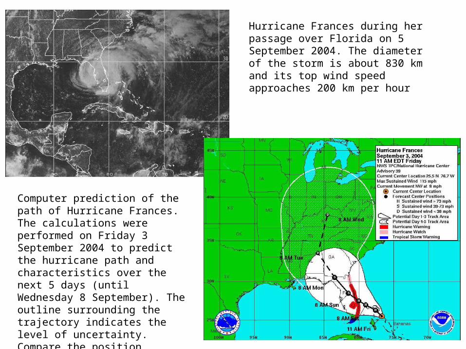
Hurricane Frances during her passage over Florida on 5 September 2004. The diameter of the storm is about 830 km and its top wind speed approaches 200 km per hour

Computer prediction of the path of Hurricane Frances. The calculations were performed on Friday 3 September 2004 to predict the hurricane path and characteristics over the next 5 days (untilWednesday 8 September). The outline surrounding the trajectory indicates the level of uncertainty.Compare the position predicted for Sunday 5 September with the actual position

Distinguishing attributes of geophysical flows

• Two main ingredients distinguish the discipline from traditional fluid mechanics: the effects of rotation and those of stratification. The controlling influence of one, the other, or both leads to peculiarities exhibited only by geophysical flows

• The presence of an ambient rotation, such as that due to the earth’s spin about its axis, introduces in the equations of motion two acceleration terms that, in the rotating framework, can be interpreted as forces. They are the Coriolis force and the centrifugal force. Although the latter is the more palpable of the two, it plays no role in geophysical flows, however surprising this may be. The former and less intuitive of the two turns out to be a crucial factor in geophysical motions

• a major effect of the Coriolis force is to impart a certain vertical rigidity to the fluid. In rapidly rotating, homogeneous fluids, this effect can be so strong that the flow displays strict columnar motions; that is, all particles along the same vertical evolve in concert, thus retaining their vertical alignment over long periods of time

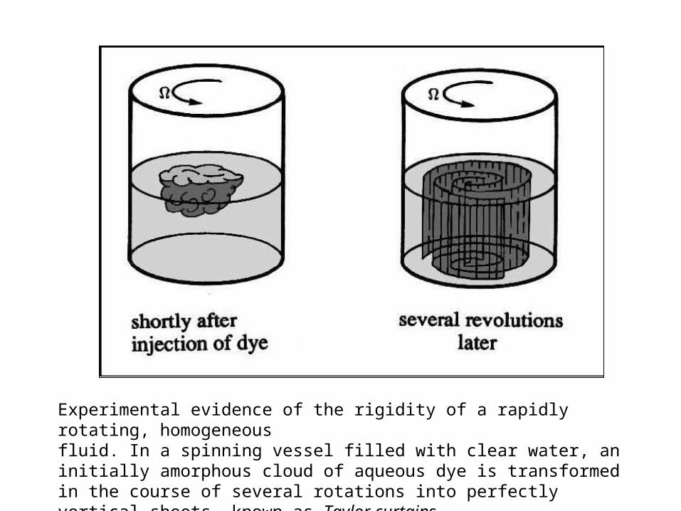
Experimental evidence of the rigidity of a rapidly rotating, homogeneousfluid. In a spinning vessel filled with clear water, an initially amorphous cloud of aqueous dye is transformed in the course of several rotations into perfectly vertical sheets, known as Taylor curtains

Scales of motions

Example – hurricane Frances 2004:• Length scale – satellite pictures revealed nearly circular feature spanning

approximately 7.5 º of latitude (830 km) L=800 km

• Velocity scale - Sustained surface wind speeds of a category-4 hurricane such as Frances range from 59 to 69 m/s

U=60 m/s• Time scale - In general, hurricane tracks display appreciable change in direction and

speed of propagation over 2-day intervalsT=2x105 s (55.6 h)

• geophysical fluids generally exhibit a certain degree of density heterogeneity, called stratification. The important parameters are:

– the average density ρ0, – the range of density variations Δ ρ– the height H over which such density variations occur

As the person new to geophysical fluid dynamics has already realized, the selection of scales for any given problem is more an art than a science. Choices are rather subjective. The trick is to choose quantities that are relevant to the problem, yet simple to establish. There is freedom. Fortunately, small inaccuracies are inconsequential because the scales are meant only to guide in the clarification of the problem, whereas grossly inappropriate scales will usually lead to flagrant contradictions. Practice, which forms intuition, is necessary to build confidence.

Importance of rotation

Ambient rotation rate:

sxrevolutionoftime

radians 51029.72

Let us define the dimensionless quantity

TTscaletimemotion

revolutiononeoftime

22

If fluid motions evolve on a time scale comparable to or longer than the time of one rotation, we anticipate that the fluid does feel the effect of the ambient rotation

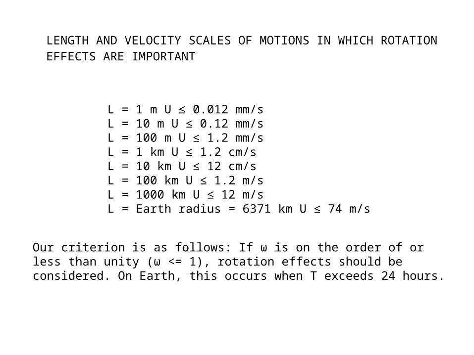
LENGTH AND VELOCITY SCALES OF MOTIONS IN WHICH ROTATION EFFECTS ARE IMPORTANT

L = 1 m U ≤ 0.012 mm/sL = 10 m U ≤ 0.12 mm/sL = 100 m U ≤ 1.2 mm/sL = 1 km U ≤ 1.2 cm/sL = 10 km U ≤ 12 cm/sL = 100 km U ≤ 1.2 m/sL = 1000 km U ≤ 12 m/sL = Earth radius = 6371 km U ≤ 74 m/s

Our criterion is as follows: If ω is on the order of or less than unity (ω <= 1), rotation effects should be considered. On Earth, this occurs when T exceeds 24 hours.

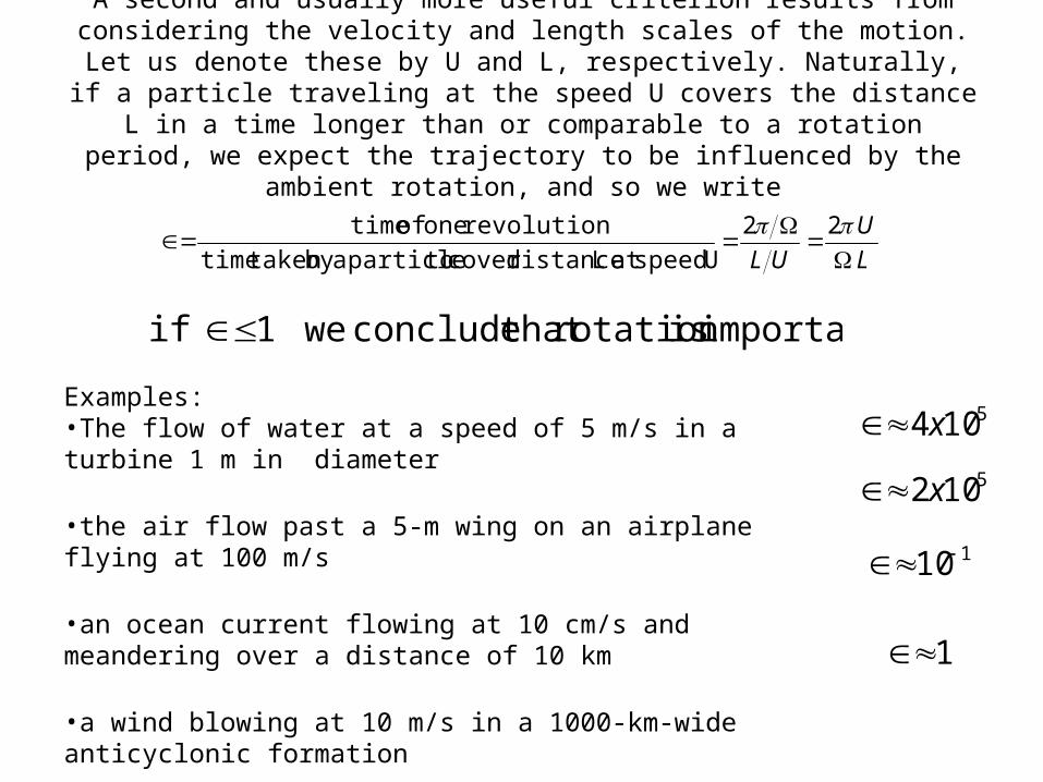
A second and usually more useful criterion results from considering the velocity and length scales of the motion. Let us denote these by U and L, respectively. Naturally, if a particle traveling at the speed U covers the distance L in a time longer than or comparable to a rotation period, we expect the trajectory to be

influenced by the ambient rotation, and so we write

L

U

UL

22

Uspeedat L distancecover toparticleabytakentime

revolutiononeoftime

important isrotation that conclude we1if

Examples:•The flow of water at a speed of 5 m/s in a turbine 1 m in diameter

•the air flow past a 5-m wing on an airplane flying at 100 m/s

•an ocean current flowing at 10 cm/s and meandering over a distance of 10 km

•a wind blowing at 10 m/s in a 1000-km-wide anticyclonic formation

5104x5102x

110

1

Importance of stratification

If Δρ is the scale of density variations in the fluid and H is its height scale, a prototypical perturbation to the stratification consists in raising a fluid element of density ρ0 + Δρ over the height H and, in order to conserve volume, lowering a lighter fluid element of density ρ0 over the same height. The corresponding change in potential energy, per unit volume, is

(ρ0+Δρ) gH −ρ0gH = ΔρgH. With a typical fluid velocity U, the kinetic energy available per unit volume is 2ρ0U2. Accordingly, we construct the comparative energy ratio

gH

U

202

1

•If σ is on the order of unity a typical potential-energy increase necessary to perturb the stratification consumes a sizable portion of the available kinetic energy, thereby modifying the flow field substantially•If σ is much less than unity, there is insufficient kinetic energy to perturb significantly the stratification, and the latter greatly constrains the flow•if σ is much greater than unity potential-energy modifications occur at very little cost to the kinetic energy, and stratification hardly affects the flow.

Combined effect of rotationa nd stratification

The most interesting situation arises in geophyscial flows when rotation and stratification are simultaneously important

1,1

HgUU

L0

,

Elimination of the velocity scale yields the fundamental length sacle

HgL0

1

typical conditions in the atmosphere (ρ0 = 1.2 kg/m3, Δρ = 0.03 kg/m3, H = 5000 m)

smUkmL atmosphereatmosphere /30,500

Typical conditions in the ocean (ρ0 = 1028 kg/m3, ρ = 2 kg/m3, H = 1000 m)

smUkmL oceanocean /4,60

Distinction between the atmosphere and oceans

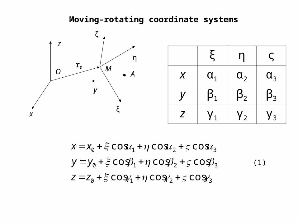
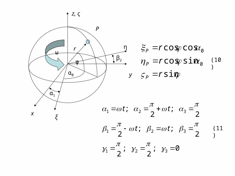
Moving-rotating coordinate systems

x

y

z

O

ξ

η

ζ

M

ξ η ς

x α1 α2 α3

y β1 β2 β3

z γ1 γ2 γ3

r0

3210

3210

3210

coscoscos

coscoscos

coscoscos

zz

yy

xx

A

(1)

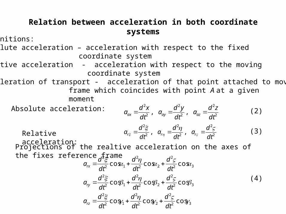
Relation between acceleration in both coordinate systems

2

2

2

2

2

2

,,dt

da

dt

da

dt

da rrr

2

2

2

2

2

2

,,dt

zda

dt

yda

dt

xda azayax

Definitions:Absolute acceleration – acceleration with respect to the fixed

coordinate systemRelative acceleration - acceleration with respect to the moving

coordinate systemAcceleration of transport - acceleration of that point attached to moving

frame which coincides with point A at a given moment

Absolute acceleration:

Relative acceleration:

Projections of the realtive acceleration on the axes of the fixes reference frame

(2)

(3)

32

2

22

2

12

2

32

2

22

2

12

2

32

2

22

2

12

2

coscoscos

coscoscos

coscoscos

dt

d

dt

d

dt

da

dt

d

dt

d

dt

da

dt

d

dt

d

dt

da

rz

ry

rx

(4)

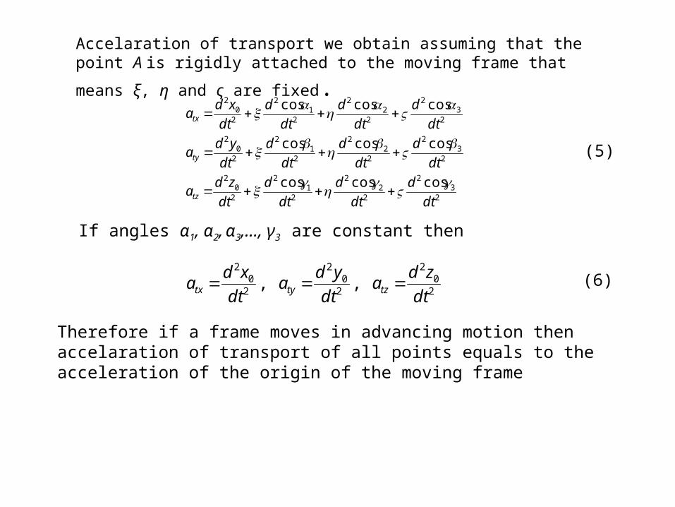
Accelaration of transport we obtain assuming that the point A is rigidly

attached to the moving frame that means ξ, η and ς are fixed.

23

2

22

2

21

2

20

2

23

2

22

2

21

2

20

2

23

2

22

2

21

2

20

2

coscoscos

coscoscos

coscoscos

dt

d

dt

d

dt

d

dt

zda

dt

d

dt

d

dt

d

dt

yda

dt

d

dt

d

dt

d

dt

xda

tz

ty

tx

(5)

If angles α1, α2, α3,…, γ3 are constant then

20

2

20

2

20

2

,,dt

zda

dt

yda

dt

xda tztytx

Therefore if a frame moves in advancing motion then accelaration of transport of all points equals to the acceleration of the origin of the moving frame

(6)

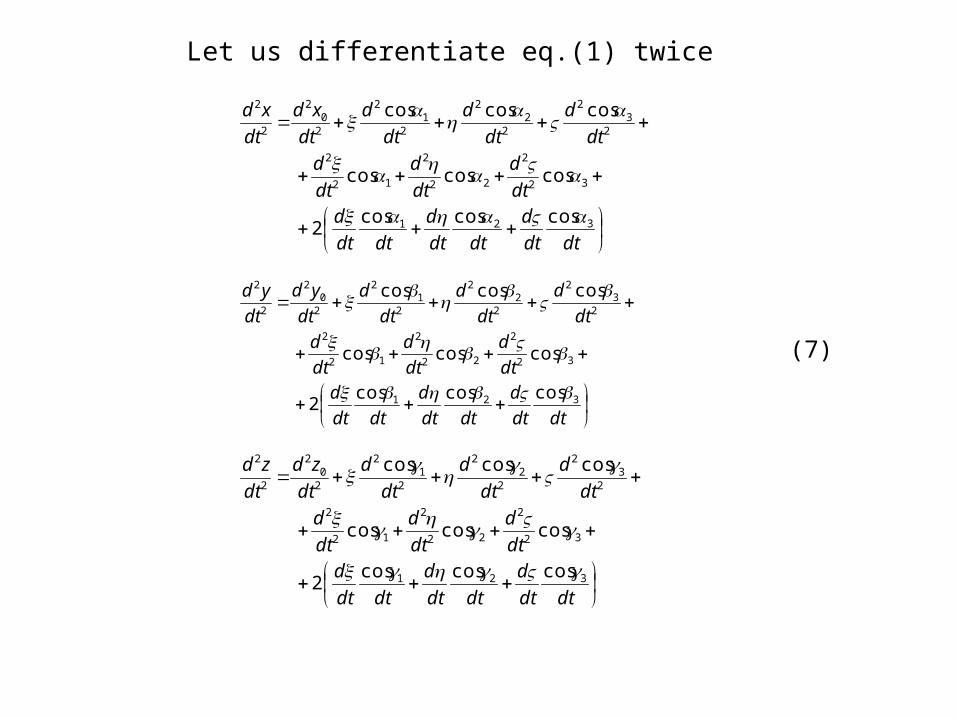
Let us differentiate eq.(1) twice

dtdt

d

dtdt

d

dtdt

ddt

d

dt

d

dt

d

dt

d

dt

d

dt

d

dt

xd

dt

xd

321

32

2

22

2

12

2

23

2

22

2

21

2

20

2

2

2

coscoscos2

coscoscos

coscoscos

dtdt

d

dtdt

d

dtdt

ddt

d

dt

d

dt

d

dt

d

dt

d

dt

d

dt

yd

dt

yd

321

32

2

22

2

12

2

23

2

22

2

21

2

20

2

2

2

coscoscos2

coscoscos

coscoscos

dtdt

d

dtdt

d

dtdt

ddt

d

dt

d

dt

d

dt

d

dt

d

dt

d

dt

zd

dt

zd

321

32

2

22

2

12

2

23

2

22

2

21

2

20

2

2

2

coscoscos2

coscoscos

coscoscos

(7)

In virtue of eqs (4) and (5) the absolute acceleration can be expressed as

Crta aaaa

Ca

Where Coriolis acceleration is

dt

d

dt

d

dt

d

dt

d

dt

d

dt

da

dt

d

dt

d

dt

d

dt

d

dt

d

dt

da

dt

d

dt

d

dt

d

dt

d

dt

d

dt

da

Cz

Cy

Cx

321

321

321

coscoscos2

coscoscos2

coscoscos2

(8)

(9)

α1

β2

P

x

y

z, ς

ξ

ηω

0;2

;2

2;;

2

2;

2;

321

321

321

tt

tt

(11)

φ

α0

r

sin

sincos

coscos

0

0

r

r

r

P

P

P

(10)

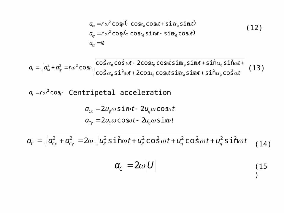
0

cossinsincoscos

sinsincoscoscos

002

002

tz

ty

tx

a

ttra

ttra

cos

cossinsinsincoscos2sincos

sinsinsinsincoscos2coscoscos

2

20

200

20

2

20

200

20

2222

ra

tttt

ttttraaa

t

tytxt

tutua

tutua

Cy

Cx

sin2cos2

cos2sin2

(12)

(13)

Centripetal acceleration

tutututuaaa CyCxC 2222222222 sincoscossin2

UaC

2

(14)

(15)

Navier-Stokes equations in the rotating reference frame

rUkgUpDtUD

21 2

(16)

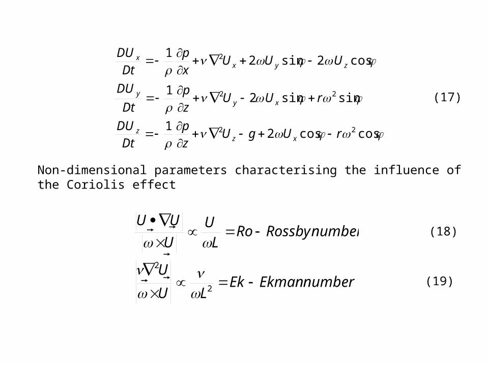
coscos21

sinsin21

cos2sin21

22

22

2

rUgUzp

DtDU

rUUzp

Dt

DU

UUUxp

DtDU

xzz

xyy

zyxx

(17)

Non-dimensional parameters characterising the influence of the Coriolis effect

numberEkmanEkLU

U

numberRossbyRoLU

U

UU

2

2

(18)

(19)

Geostrophic flow

Consider a steady flow in which the Coriolis effect is large compared with both the inertia of the relative motion and viscous forces (Ro<<1, Ek<<1)

pU

12

(20)

Flows in which this balance of forces between Corriolis effects and prssure gradinet forces is dominant are called

Geostrophic Flows

sin2

sin2

x

y

Uy

p

Ux

p

(21)

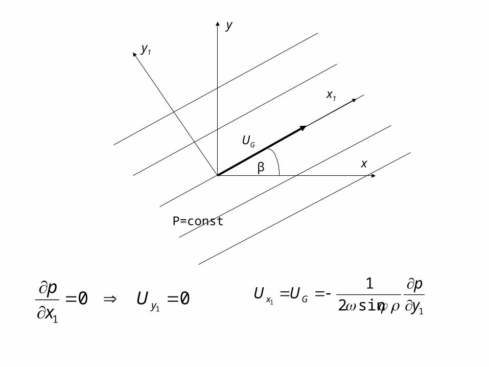
0sinsin

yxxyyx UUUUU

yp

Uxp

Up

Up

(22)

P=const

β x

y

x1

y1

UG

001

1

yUx

p1sin2

11 y

pUU Gx

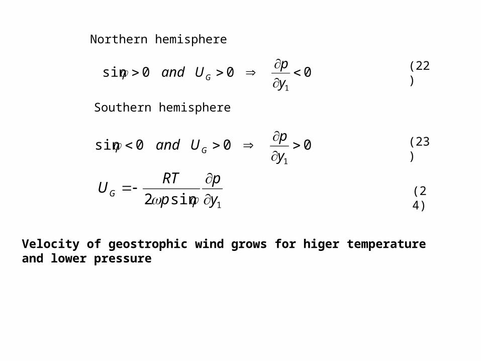
000sin1

y

pUand G

000sin1

y

pUand G

Northern hemisphere

Southern hemisphere

1sin2 y

p

p

RTUG

(22)

(23)

(24)

Velocity of geostrophic wind grows for higer temperature and lower pressure

Scale of motionIt is generally not required to discriminate between the two horizontal directions, and we assign the same length scale L to both coordinates and the same velocity scale U to both velocity components. The same, however, cannot be said of the vertical direction. Geophysical flows are typically confined to domains that are much wider than they are thick, and the aspect ratio H/L is small. The atmospheric layer that determines our weather is only about 10 km thick, yet cyclones and anticyclones spread over thousands of kilometers. Similarly, ocean currents are generally confined to the upper hundred meters of the water column but extend over tens of kilometers or more, up to the width of the ocean basin.

LH For large scale motion

Hence we expect that Uz is much different from Ux and Uy

The continuity equation contains three terms, of respective orders of magnitude:

H

W

L

U

L

U,,

We ought to examine three cases: W/H is much less than, on the order of, or much greater than U/L.

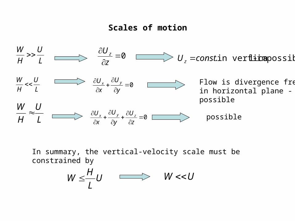
Scales of motion

L

U

H

W 0

z

U zimpossible - lin vertica .constU z

L

U

H

W 0

y

U

x

U yx Flow is divergence free in horizontal plane - possible

L

U

H

W

0

z

U

y

U

x

U zyx possible

In summary, the vertical-velocity scale must be constrained by

UL

HW UW

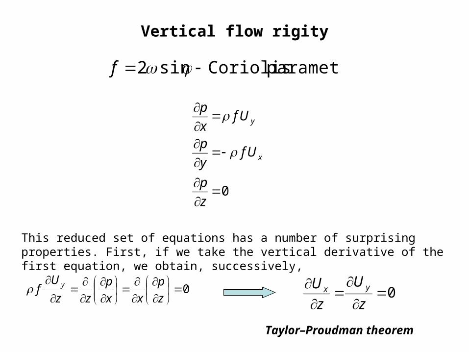
Vertical flow rigity

parameter Coriolis sin2 f

0

z

p

Ufy

p

Ufx

p

x

y

0

z

p

xx

p

zz

Uf y

This reduced set of equations has a number of surprising properties. First, if we take the vertical derivative of the first equation, we obtain, successively,

0

z

U

z

U yx

Taylor–Proudman theorem

Taylor-Proudman theorem

Physically, it means that the horizontal velocity field has no vertical shear and that all particles on the same vertical move in concert. Such vertical rigidity is a fundamental property of Rotating homogeneous fluids.

Homogeneous geostrophic flows over an irregular bottom

This property has profound implications. In particular, if the topography consists of an isolated bump (or dip) in an otherwise flat bottom, the fluid on the flat bottom cannot rise onto the bump, even partially, but must instead go around it. Because of the vertical rigidity of the flow, the fluid parcels atall levels – including levels above the bump elevation – must likewise go around. Similarly, the fluid over the bump cannot leave the bump but must remain there. Such permanent tubes of fluids trapped above bumps or cavities are called Taylor columns (Taylor, 1923).

Geostrophic flow in a closed domain and over irregular topography. Solid lines are isobaths (contours of equal depth). Flow is permitted only along closed isobaths.

Gradient windGeostrophic winds exist in locations where there are no frictional forces and the isobars are straight. However, such locations are quite rare. Isobars are almost always curved and are very rarely evenly spaced. This changes the geostrophic winds so that they are no longer geostrophic but are instead in gradient wind balance. They still blow parallel to the isobars, but are no longer balanced by only the pressure gradient and Coriolis forces, and do not have the same velocity as geostrophic winds.

Low pressure

cyclone

high pressure

anticyclone

Centrifugal force

Coriolis force Ug

Pressure gradient Coriolis force

Ug

Centrifugal force

Pressure gradient

Let us introduce the polar coordinate system with the origin in the point of maximum/minimum pressure

sin2111

sin211 2

rr

r

rrr

Up

rr

UUU

rU

r

UU

Ur

p

r

UU

rU

r

UU

0p

0,0

UU r

(25a)

In the case when isobars have circular shape

To satisfy Eq.(25b)

(25b)

r

pU

r

U

1

sin22

(26)

Gradient wind solution

tcoefficien Coriolis - sin2 where,02

fr

prrUfU (27)

r

p

rf

frfrU

2

41

22

Constraints on the gradient wind solution:

•In Eq.(26), r ∞ the centrifugal term becomes negligible and geostrophic balance is retrieved. That imposes a constraint on waht solutions are physically acceptable: they must yield the geostrophic wind solution in the limit of large curvature radius

•The solution must be real

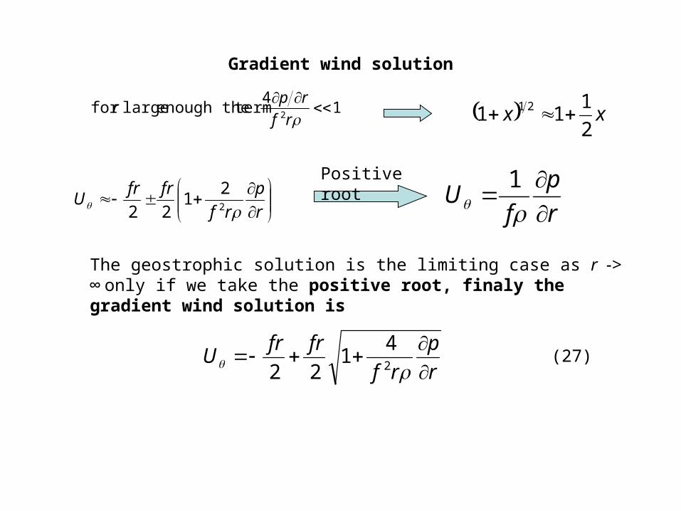
Gradient wind solution

14

termenough the large for 2

rfrp

r xx2

111 21

r

p

rf

frfrU

2

21

22

Positive root

r

p

fU

1

The geostrophic solution is the limiting case as r -> ∞ only if we take the positive root, finaly the gradient wind solution is

r

p

rf

frfrU

2

41

22(27)

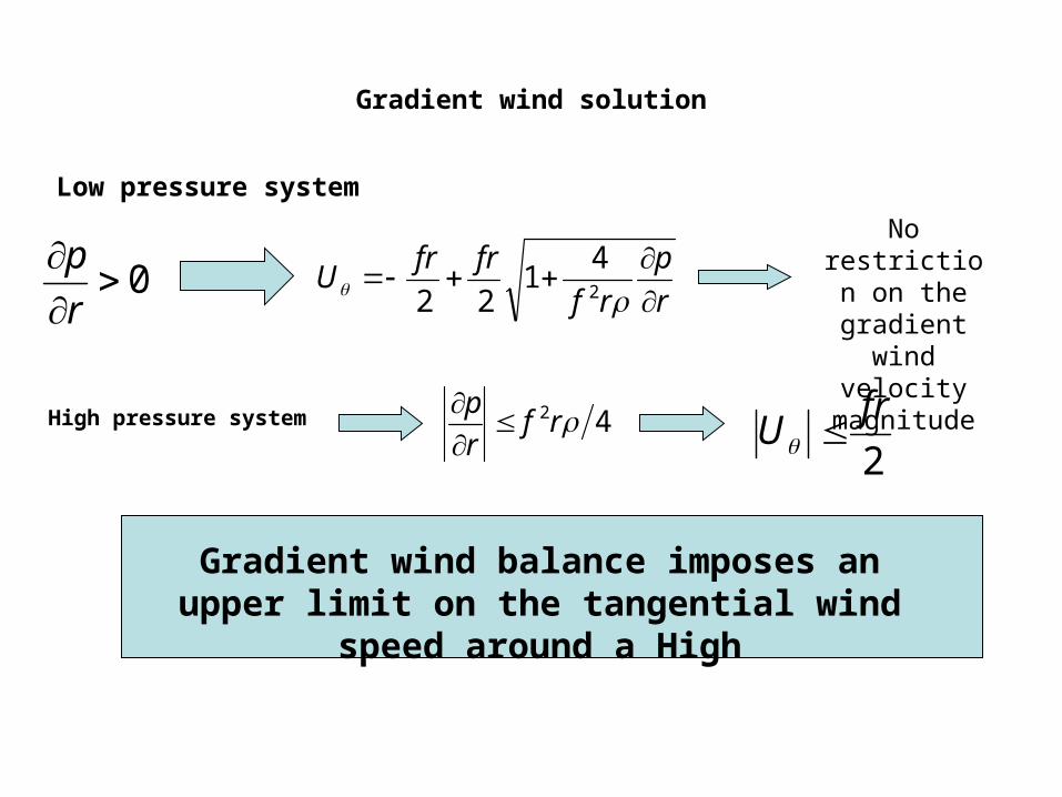
Gradient wind solution

Low pressure system

0r

pr

p

rf

frfrU

2

41

22

No restriction on the

gradient wind velocity

magnitude

High pressure system 42 rfr

p

2

frU

Gradient wind balance imposes an upper limit on the tangential wind speed around a High

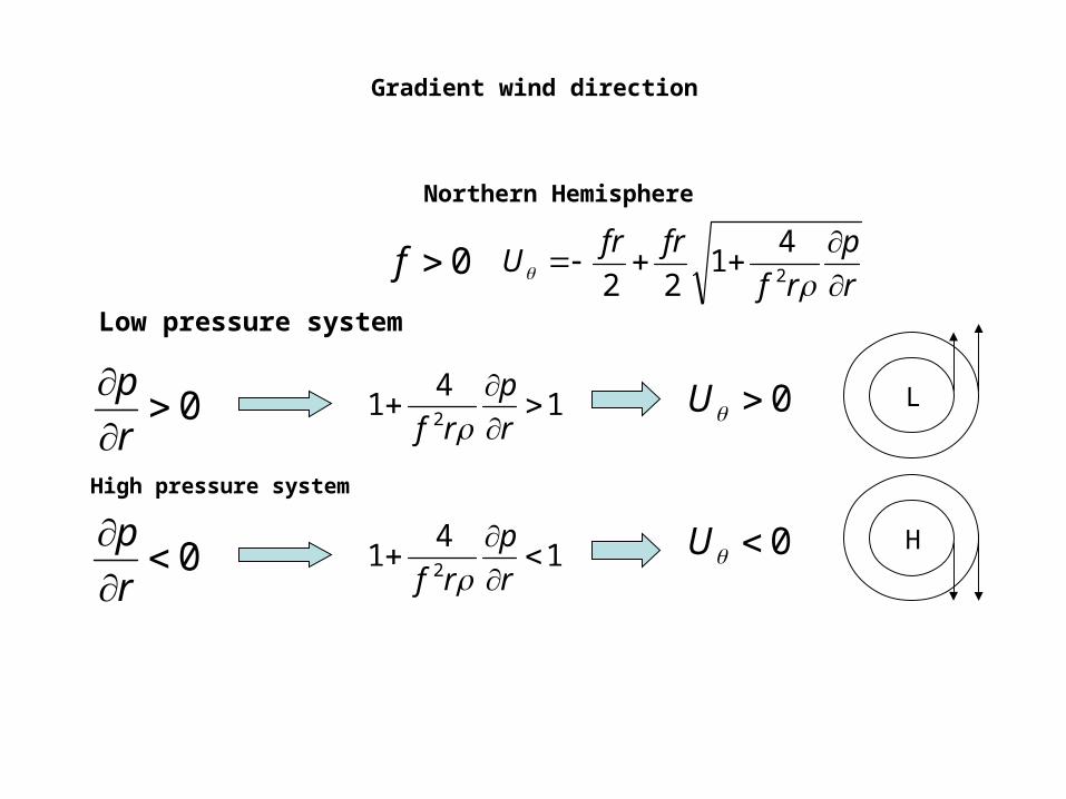
Gradient wind direction

Northern Hemisphere

r

p

rf

frfrU

2

41

220f

Low pressure system

0r

p1

41

2

r

p

rf 0U L

High pressure system

0r

p1

41

2

r

p

rf 0U H

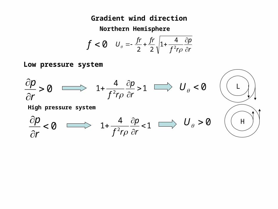
Northern Hemisphere

0f

Low pressure system

0r

p1

41

2

r

p

rf 0U L

High pressure system

0r

p1

41

2

r

p

rf 0U H

r

p

rf

frfrU

2

41

22

Gradient wind direction

rf

U

r

p

fU

21

Gradient wind magnitude

rf

UU

r

U

r

p

fU

L

G

LL

2211

G

L UU

rf

UHU

r

U

r

p

fU G

HH

2211

GH UU

(28)

(29a)

(29b)

Conclusion:

With the same horizontal pressure gradient the cyclonic gradient wind speed is lower than anticyclonic one

Ekman layer

B

zUA

U

zU

*

*

ln *** 2.5ln UzU

K

UzU

Logarithmic profile- non-rotating flow

or (30)

(31)Where:

constantKarman von - 0.411

elocityfriction v - *

AK

U b

(32)

Mean velocity profiles in fully developed turbulent channel flow measured byWei andWillmarth (1989) at various Reynolds numbers: circles Re = 2970, squares Re = 14914, upright triangles Re = 22776, and downright triangles Re = 39582. The straight line on this log-linear plot corresponds to the logarithmic profile of Equation (8.2). (From Pope, 2000)

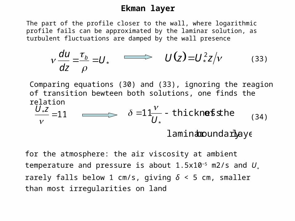
The part of the profile closer to the wall, where logarithmic profile fails can be approximated by the laminar solution, as turbulent fluctuations are damped by the wall presence

*Udz

du b

Ekman layer

zUzU 2* (33)

Comparing equations (30) and (33), ignoring the reagion of transition bewteen both solutions, one finds the relation

11* zU

layerboundary laminar

theof thickness- 11*U

for the atmosphere: the air viscosity at ambient temperature and pressure is

about 1.5x10−5 m2/s and U∗ rarely falls below 1 cm/s, giving δ < 5 cm,

smaller than most irregularities on land

(34)

Ekman layer

Velocity profile in the vicinity of a rough wall. The roughness heigh z0 is smaller than the averaged height of the surface asperities. So, the velocity u falls to zero somewhere within the asperities, where local flow degenerates into small vortices between the peaks, and the negative values predicted by the logarithmic profile are not physically realized.

When this is the case, the velocity profile above the bottom asperities no longer depends on the molecular viscosity of the fluid but on the so-called roughness height z0, such that

0

* lnz

z

K

UzU (35)

Ekman layer

Eddy viscosity

In analogy with Newton’s law for viscous fluids, which has the tangential stress τ proportional to the velocity shear du/dz with the coefficient of proportionality being the molecular viscosity ν, we write for turbulent flow:

dz

zdUT

Kz

U

dz

zdU *

2*Ub

(36)

For the logaritmic velocity profile of a flow along the rough surface the velocity shear is

and the stress τ is uniform across the flow (at least in the vicinity of the boundary for lack of other significant forces), hence

(37)

(38)giving

length mixing Prandtl - where

- ***2

*

m

mTTT

l

UlKzUKz

UU

(39)

Ekman layer

Friction and rotation

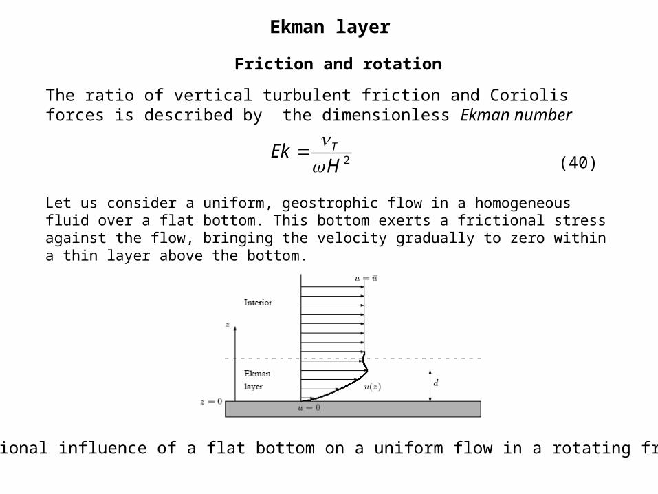
The ratio of vertical turbulent friction and Coriolis forces is described by the dimensionless Ekman number

2HEk T

(40)

Let us consider a uniform, geostrophic flow in a homogeneous fluid over a flat bottom. This bottom exerts a frictional stress against the flow, bringing the velocity gradually to zero within a thin layer above the bottom.

Frictional influence of a flat bottom on a uniform flow in a rotating framework.

Ekman layer

z

p

z

U

y

pUf

z

U

x

pUf

yTx

xTy

10

1

1

2

2

2

2

U

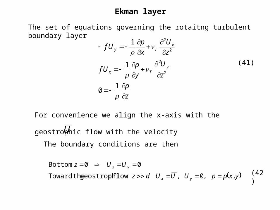
The set of equations governing the rotaitng turbulent boundary layer

(41)

For convenience we align the x-axis with the geostrophic flow with the

velocity

The boundary conditions are then

yxppUUUdz

UUz

yx

yx

,,0, :flow cgeostrophi theToward

00 :Bottom

(42)

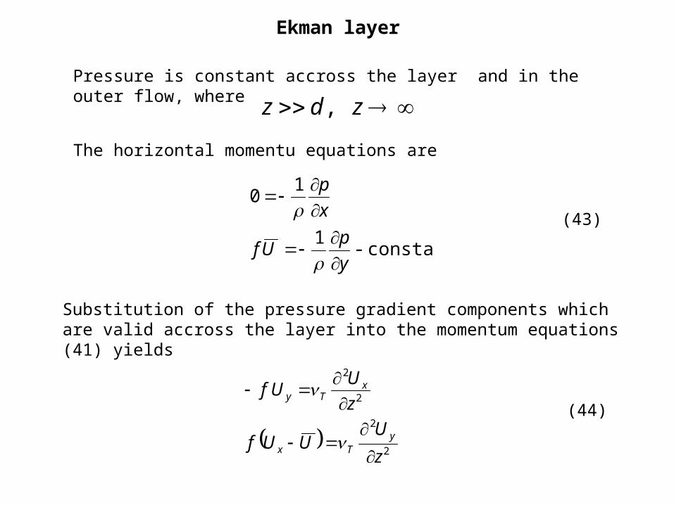
Ekman layer

Pressure is constant accross the layer and in the outer flow, where

zdz ,

constant - 1

10

y

pUf

x

p

The horizontal momentu equations are

(43)

Substitution of the pressure gradient components which are valid accross the layer into the momentum equations (41) yields

2

2

2

2

z

UUUf

z

UUf

yTx

xTy

(44)

Ekman layer

Looking for the solution of Eq. (44) one can note that

2

2

dz

Ud

fUU yT

x

04

4

2

2

yyT U

dz

Ud

f

41

2

2242 0

TT

ff

(45)

Substitution of Eq.(45) into first of Eqs (44) leads to

(46)

Looking for a solution of Eq.(46) in the form

(47)

Substitution of the particular solution (47) into Eq. (46) leads to condition

4

7exp;

4

5exp;

4

3exp;

4exp

24exp

21

3

21

3

21

2

21

1

21

if

if

if

if

kif

TTTT

T

(48)

zCU y exp

Ekman layer

2

1

2

1;

2

1

2

1;

2

1

2

1;

2

1

2

14321 i

fi

fi

fi

f

TTTT

d

i1

1

fd T2

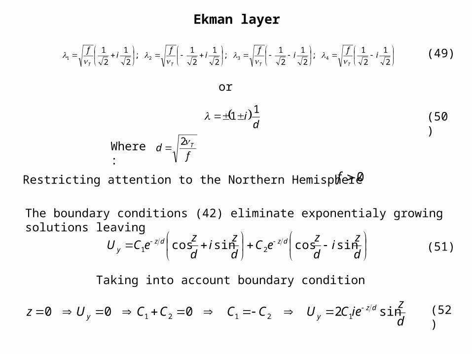
(49)

or

(50)

Where:

Restricting attention to the Northern Hemisphere 0f

The boundary conditions (42) eliminate exponentialy growing solutions leaving

d

zi

d

zeC

d

zi

d

zeCU dzdz

y sincossincos 21 (51)

Taking into account boundary condition

d

zieCUCCCCUz dz

yy sin2000 12121 (52)

Ekman layer

d

ze

d

iC

d

z

d

ze

dd

z

d

ze

dd

iC

dz

Ud

d

z

d

ze

d

iC

dz

dU

dzdzdzy

dzy

cos4

sincos1

cossin12

cossin2

211

2

2

1

d

zeiCUU dz

x cos2 1

i

UCUiCUz x 2

200 11

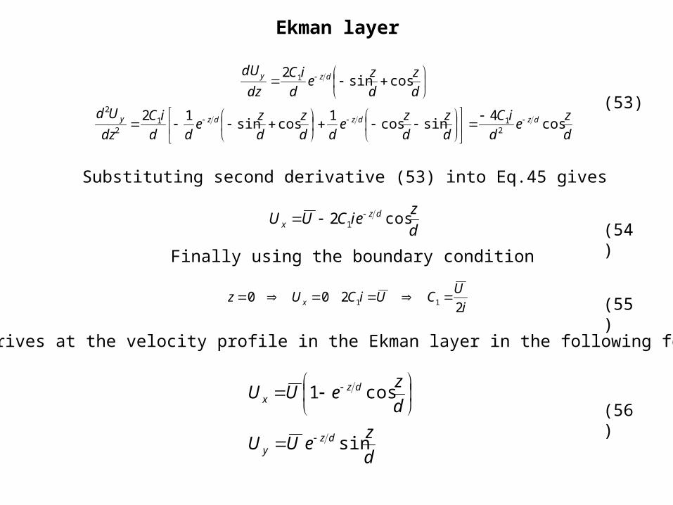
(53)

Substituting second derivative (53) into Eq.45 gives

(54)

Finally using the boundary condition

One arrives at the velocity profile in the Ekman layer in the following form

d

zeUU

d

zeUU

dzy

dzx

sin

cos1

(55)

(56)

Ekman layer

The velocity spiral in the bottom Ekman layer. The figure is drawn for the Northern Hemisphere (f > 0), and the deflection is to the left of the current above the layer. The reverse holds for the Southern Hemisphere.

This solution has a number of important properties. First and foremost, we notice that the distance over which it approaches the interior solution is on the order of d. Thus d gives the thickness of the boundary layer. For this reason, d is called the Ekman depth. A comparison with (40) confirms the earlier argument that the boundary-layer thickness is the one corresponding to a local Ekman number near unity.

d

zUUUz yx 0

Ekman layer

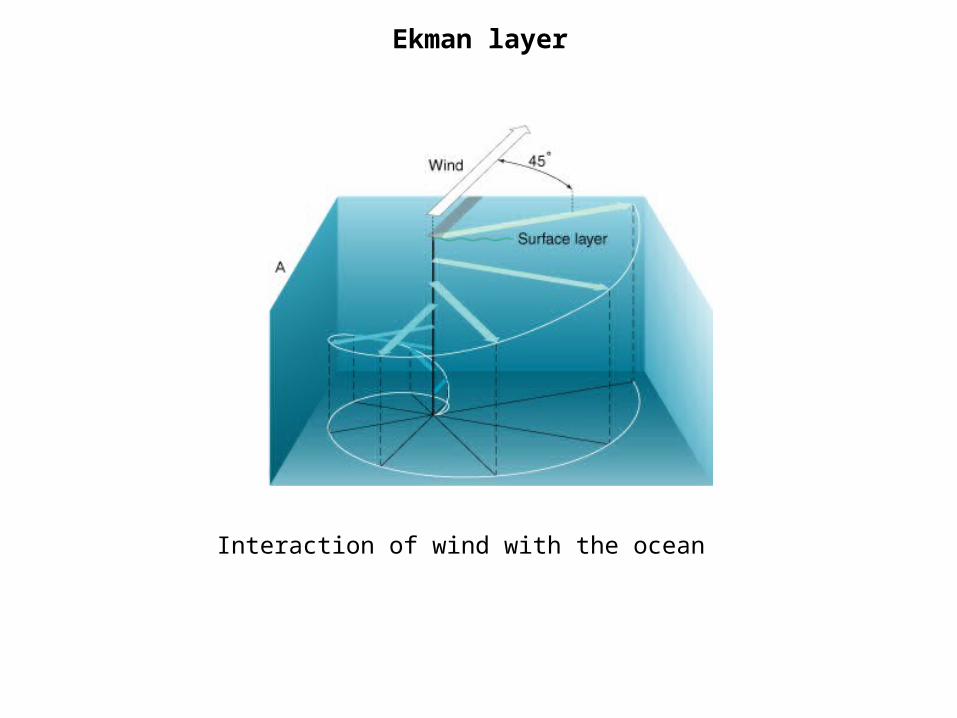
Interaction of wind with the ocean

Stratification

As stated, problems in geophysical fluid dynamics concern fluid motions with one or both of two attributes, namely, ambient rotation and stratification. In the preceding chapters, attention was devoted exclusively to the effects of rotation, and stratification was avoided by the systematic assumption of a homogeneous fluid. We noted that rotation imparts to the fluid a strong tendency to behave in a columnar fashion— to be vertically rigid.

By contrast, a stratified fluid, consisting of fluid parcels of various densities, will tend under gravity to arrange itself so that the higher densities are found below lower densities. This vertical layering introduces an obvious gradient of properties in the vertical direction, which affects—among other things—the velocity field. Hence, the vertical rigidity induced by the effects of rotation will be attenuated by the presence of stratification. In return, the tendency of denser fluid to lie below lighter fluid imparts a horizontal rigidity to the system.

Static stability

When an incompressible fluid parcel of density (z) is vertically displaced from level z to level z + h in a stratified environment, a buoyancy force appears because of the density difference (z)−(z+h) between theparticle and the ambient fluid

Stratification

If the fluid is incompressible, our displaced parcel retains its former density despite a slight pressure change, and at that new level is subject to a net downward force equal to its own weight minus, by Archimedes’ buoyancy principle, the weight of the displaced fluid, thus

where V is the volume of the parcel. As it is written, this force is positive if it is directed downward. Newton’s law (mass times acceleration equals upward force) yields

Vhzzg

zhzgdt

hdVz

2

2

(57)

(58)

As the density differences in geophysical flow are weak we can use Boussinesq approximation

dz

dgN

hNdt

thdh

dz

dg

dt

thd

0

2

22

2

02

2

where

00

(59)

Stratification

tth exp

222 0 NN

Assuming the solution with respect to time in the form

(60)

and introducing this solution into the differential equation one obtains

(61)

solution unstable - and 0 0 if 212 NtNt eCeCthN

dz

d

(62)

frequency, Vaisala–Brunt where

motiony oscillator - sincos and

0 0 if

11

2

N

NtiNtCeCth

Ndz

d

iNt

(63)

Stratification

Typical profile of potential temperature in the lower atmosphere above warm ground

Importance of stratification

The time passed in the vicinity of the obstacle is approximately the time spent by a fluid parcel to cover the horizontal distance L at the speed U, that is, T = L/U. To climb a height of z, the fluid needs to acquire a vertical velocity on the order of

T

zU

T

zW

(64)

Importance of stratification

zg

Nz

dz

d

20

zHNgHp 20

x

p

y

UU

x

UU x

yx

x

0

1

The vertical displacement is on the order of the height of the obstacle and, in the presence of stratification ρ(z), causes a density perturbation on the order of

(65)

In turn, this density variation gives rise to a pressure disturbance that scales, via the hydrostatic balance, as

(66)

By virtue of the balance of forces in the horizontal, the pressure-gradient force must be accompanied by a change in fluid velocity

zHNUL

p

L

U

22

0

2

(67)

(68)

Importance of stratification

22

2

/

/ (68) Eq. from and

/

/

HN

U

LU

HW

H

z

LU

HW

z

U

y

U

x

U zyx

-byn better tha -by balanced becan

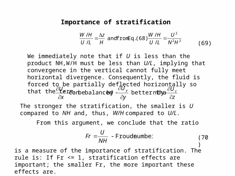
(69)

We immediately note that if U is less than the product NH,W/H must be less than U/L, implying that convergence in the vertical cannot fully meet horizontal divergence. Consequently, the fluid is forced to be partially deflected horizontally so that the term

The stronger the stratification, the smaller is U compared to NH and, thus, W/H compared to U/L.

From this argument, we conclude that the ratio

number Froude - NH

UFr (70)

is a measure of the importance of stratification. The rule is: If Fr <= 1, stratification effects are important; the smaller Fr, the more important theseeffects are.

Combination of rotation and stratification

L

zHNU

L

pU

2

0

From geostrophic balance we have

(71)

The ratio of the vertical to horizontal convergence then becomes

Ro

Fr

HN

LU

H

z

LU

HW 2

22

(72)

Combination of rotation and stratification