Liqun Qi Haibin Chen Yannan Chen Tensor Eigenvalues and ...
336
Advances in Mechanics and Mathematics 39 Liqun Qi Haibin Chen Yannan Chen Tensor Eigenvalues and Their Applications
Transcript of Liqun Qi Haibin Chen Yannan Chen Tensor Eigenvalues and ...

Advances in Mechanics and Mathematics 39
Liqun QiHaibin ChenYannan Chen
Tensor Eigenvalues and Their Applications
Advances in Mechanics and Mathematics
Volume 39
More information about this series at http://www.springer.com/series/5613
Series Editors
David Gao, Federation University AustraliaTudor Ratiu, Shanghai Jiao Tong University
Advisory Board
Antony Bloch, University of MichiganJohn Gough, Aberystwyth UniversityDarryl D. Holm, Imperial College LondonPeter Olver, University of MinnesotaJuan-Pablo Ortega, University of St. GallenGenevieve Raugel, CNRS and University Paris-SudJan Philip Solovej, University of CopenhagenMichael Zgurovsky, Igor Sikorsky Kyiv Polytechnic InstituteJun Zhang, University of MichiganEnrique Zuazua, Universidad Autónoma de Madrid and DeustoTech

Liqun Qi • Haibin Chen • Yannan Chen
Tensor Eigenvalues and TheirApplications
123

Liqun QiDepartment of Applied MathematicsThe Hong Kong Polytechnic UniversityHong KongHong Kong
Haibin ChenSchool of Management SciencesQufu Normal UniversityRizhao, ShandongChina
Yannan ChenThe Hong Kong Polytechnic UniversityHong KongHong Kong
ISSN 1571-8689 ISSN 1876-9896 (electronic)Advances in Mechanics and MathematicsISBN 978-981-10-8057-9 ISBN 978-981-10-8058-6 (eBook)https://doi.org/10.1007/978-981-10-8058-6
Library of Congress Control Number: 2018934953
© Springer Nature Singapore Pte Ltd. 2018This work is subject to copyright. All rights are reserved by the Publisher, whether the whole or partof the material is concerned, specifically the rights of translation, reprinting, reuse of illustrations,recitation, broadcasting, reproduction on microfilms or in any other physical way, and transmissionor information storage and retrieval, electronic adaptation, computer software, or by similar or dissimilarmethodology now known or hereafter developed.The use of general descriptive names, registered names, trademarks, service marks, etc. in thispublication does not imply, even in the absence of a specific statement, that such names are exempt fromthe relevant protective laws and regulations and therefore free for general use.The publisher, the authors and the editors are safe to assume that the advice and information in thisbook are believed to be true and accurate at the date of publication. Neither the publisher nor theauthors or the editors give a warranty, express or implied, with respect to the material contained herein orfor any errors or omissions that may have been made. The publisher remains neutral with regard tojurisdictional claims in published maps and institutional affiliations.
Printed on acid-free paper
This Springer imprint is published by the registered company Springer Nature Singapore Pte Ltd. part ofSpringer NatureThe registered company address is: 152 Beach Road, #21-01/04 Gateway East, Singapore 189721,Singapore

Preface
Tensors, as geometric objects that describe linear or multi-linear relations betweengeometric vectors, scalars, and other tensors, have provided a concise mathematicalframework for formulating and solving practical physics problems in various areassuch as relativity theory, fluid dynamics, solid mechanics, electromagnetism, etc.The concept of tensors can be traced back to the works by Carl Friedrich Gauss(1777–1855), Bernhard Riemann (1826–1866), Elwin Bruno Christoffel (1829–1900), etc., in the nineteenth century on differential geometry. It was furtherdeveloped and analyzed by Gregorio Ricci-Curbastro (1853–1925), TullioLevi-Civita (1873–1941), and others, in the very beginning of the twentieth cen-tury. A mathematical discipline on tensor analysis gradually emerged and was evenapplied in general relativity by the great scientist Albert Einstein (1879–1955) in1916. This not only shows the great power of tensor analysis in theoretical physicsbut also starts the journey to widespread applications in continuum mechanics andmany other areas in science and engineering.
When a coordinate basis or a frame of reference is given, a tensor can berepresented as an organized multidimensional array of numerical values. In thiscase, tensors are treated as hypermatrices which are exactly the higher order gen-eralization of matrices. Tensors that have been relatively systematically treated inthe book Tensor Analysis: Spectral Theory and Special Tensors by Liqun Qi andZiyan Luo [228] are actually hypermatrices. As for a great majority of references intensor decomposition, tensor spectral theory, and spectral hypergraph theory, theword “tensor” is widely used for those multidimensional arrays. Following thishabit, we will adopt the terminology of “tensor” both for multidimensional arraysand tensors as physical quantities. Different from the main concerns in the book[228] where great emphasis has been addressed on properties of tensor eigenvaluesand special structured tensors in the setting of hypermatrices, more applications oftensors in both of the aforementioned two settings will be explored and discussed.These applications include multi-linear systems in numerical algebra, exponential
v

data fitting in data science, tensor complementarity problems and tensor eigenvaluecomplementarity problems in optimization, higher order diffusion tensor imaging inmedical imaging, liquid crystal study, piezoelectric effects, solid mechanics,quantum entanglement problems, etc. We hope that this book may provide a goodbase for further research on tensor eigenvalue applications in these and some moreareas.
This book is divided into nine chapters. In Chap. 1, some preliminaries of tensoreigenvalues are given. In Chaps. 2–5, tensors are treated as hypermatrices just likein the book Tensor Analysis: Spectral Theory and Special Tensors, and moretheoretical and practical applications are discussed. In the last four chapters, tensorstake its original form of physical quantities and applications of tensors eigenvaluesin physics and mechanics are elaborated, with a special and careful treatment onthird-order tensors due to its important applications in physics and its nice prop-erties in theoretical aspect, as seen in Sect. 7.1.
While tensors such as piezoelectric tensors and elasticity tensors have been usedin physics and mechanics for more than one century, the study on spectral prop-erties of these tensors is still very new. The fundamental principle of Galileo Galilei(1564–1642), who has played a pioneer role in the scientific revolution of theseventeenth century and is regarded as the father of science, is to study the rules andinsights of the nature, while mathematics is the basic tool in this process. Inspiredby this principle, the mathematical analysis on spectral properties will be stated forsuch tensors in physics and mechanics, aiming to get a better understanding in theinvolved applications. More spectral properties of tensors in physics and mechanicsawait being exploited even after this book.
We are grateful to David Gao and Ratiu Tudor for their support to include thisbook in their Springer book series “Advances in Mechanics and Mathematics”. Weare thankful to Ramon Peng for his excellent editorial work. We are also grateful toJingya Chang, Weiyang Ding, Zhenghai Huang, Ziyan Luo, Guofeng Zhang, ChenLing, Yisheng Song, Shenglong Hu, Chen Ouyang, Jinjie Liu, Changqing Xu, LejiaGu, and Zhongming Chen for their comments and proofreading of this book, and toLieven De Lathauwer, Andrzej Cichocki, Kungching Chang, Avi Berman,Qingwen Wang, Donghui Li, Xiaoqing Jin, Lixing Han, Wen Li, Michael Ng,Jinyan Fan, Jiawang Nie, Yaotang Li, Chaoqian Li, and many others for theirencouragements and supports. We are also thankful to our other research collab-orators Yimin Wei, Maolin Che, Naihua Xiu, Seetharama Gowda, Hongjin He,Gaohang Yu, Yiju Wang, Deren Han, Ed Wu, Yuhong Dai, Hongyan Ni, Yi Xu,Epifanio Virga, Antal Jákli, Huihui Dai, Xinzhen Zhang, Hong Yan, Hua Xiang,Guyan Ni, Minru Bai, Daniel Braun, Fabian Bohnet-Waldraff, Olivier Giraud, etc.In particular, we have benefited from our discussion with Bernd Sturmfels oneigendiscriminants, and our discussion with Quanshui Zheng on mechanics.
Liqun Qi’s work was supported by the Hong Kong Research Grant Council(Grant No. PolyU 501913, 15302114, 15300715, and 15301716). Haibin Chen’swork was supported by the National Natural Science Foundation of China (Grant
vi Preface
No. 11601261) and Natural Science Foundation of Shandong Province (GrantNo. ZR2016AQ12). Yannan Chen’s work was supported by the National NaturalScience Foundation of China (Grant No. 11401539, 11771405).
Hong Kong, Hong Kong Liqun QiQufu, China Haibin ChenHong Kong, Hong Kong Yannan ChenSeptember 2017
Preface vii

Contents
1 Preliminaries . . . . . . . . . . . . . . . . . . . . . . . . . . . . . . . . . . . . . . . . . . . 11.1 Tensors (Hypermatrices) and Tensor Products . . . . . . . . . . . . . . 11.2 Eigenvalues of Tensors . . . . . . . . . . . . . . . . . . . . . . . . . . . . . . . 41.3 Notes . . . . . . . . . . . . . . . . . . . . . . . . . . . . . . . . . . . . . . . . . . . . 7
2 Multilinear Systems . . . . . . . . . . . . . . . . . . . . . . . . . . . . . . . . . . . . . 92.1 Multilinear Systems Defined by M-Tensors . . . . . . . . . . . . . . . . 102.2 Finding the Positive Solution of a Nonsingular M-Equation . . . . 162.3 Tensor Methods for Solving Symmetric M-Tensor Systems . . . . 252.4 Solution Methods for General Multilinear Systems . . . . . . . . . . . 352.5 Notes . . . . . . . . . . . . . . . . . . . . . . . . . . . . . . . . . . . . . . . . . . . . 442.6 Exercise . . . . . . . . . . . . . . . . . . . . . . . . . . . . . . . . . . . . . . . . . . 47
3 Hankel Tensor Computation and Exponential Data Fitting . . . . . . . 493.1 Fast Hankel Tensor–Vector Product . . . . . . . . . . . . . . . . . . . . . . 503.2 Computing Eigenvalues of a Hankel Tensor . . . . . . . . . . . . . . . . 533.3 Convergence Analysis . . . . . . . . . . . . . . . . . . . . . . . . . . . . . . . . 563.4 Exponential Data Fitting . . . . . . . . . . . . . . . . . . . . . . . . . . . . . . 603.5 Notes . . . . . . . . . . . . . . . . . . . . . . . . . . . . . . . . . . . . . . . . . . . . 633.6 Exercises . . . . . . . . . . . . . . . . . . . . . . . . . . . . . . . . . . . . . . . . . 64
4 Tensor Complementarity Problems . . . . . . . . . . . . . . . . . . . . . . . . . . 654.1 Preliminaries for Tensor Complementarity Problems . . . . . . . . . . 674.2 An m Person Noncooperative Game . . . . . . . . . . . . . . . . . . . . . 704.3 Positive Definite Tensors for Tensor Complementarity
Problems . . . . . . . . . . . . . . . . . . . . . . . . . . . . . . . . . . . . . . . . . 784.4 P and P0-Tensors . . . . . . . . . . . . . . . . . . . . . . . . . . . . . . . . . . . 834.5 Tensor Complementarity Problems and Semi-positive
Tensors . . . . . . . . . . . . . . . . . . . . . . . . . . . . . . . . . . . . . . . . . . 924.6 Tensor Complementarity Problems and Q-Tensors . . . . . . . . . . . 984.7 Z-Tensor Complementarity Problems . . . . . . . . . . . . . . . . . . . . . 110
ix

4.8 Solution Boundedness of Tensor ComplementarityProblems . . . . . . . . . . . . . . . . . . . . . . . . . . . . . . . . . . . . . . . . . 116
4.9 Global Uniqueness and Solvability . . . . . . . . . . . . . . . . . . . . . . 1224.10 Exceptional Regular Tensors and Tensor Complementarity
Problems . . . . . . . . . . . . . . . . . . . . . . . . . . . . . . . . . . . . . . . . . 1264.11 Notes . . . . . . . . . . . . . . . . . . . . . . . . . . . . . . . . . . . . . . . . . . . . 1334.12 Exercises . . . . . . . . . . . . . . . . . . . . . . . . . . . . . . . . . . . . . . . . . 134
5 Tensor Eigenvalue Complementarity Problems . . . . . . . . . . . . . . . . . 1355.1 Tensor Eigenvalue Complementarity Problems . . . . . . . . . . . . . . 1375.2 Pareto H(Z)-Eigenvalues of Tensors . . . . . . . . . . . . . . . . . . . . . . 1475.3 Computational Methods for Tensor Eigenvalue
Complementarity Problems . . . . . . . . . . . . . . . . . . . . . . . . . . . . 1505.4 A Unified Framework of Tensor Higher-Degree Eigenvalue
Complementarity Problems . . . . . . . . . . . . . . . . . . . . . . . . . . . . 1585.5 The Semidefinite Relaxation Method . . . . . . . . . . . . . . . . . . . . . 1695.6 Notes . . . . . . . . . . . . . . . . . . . . . . . . . . . . . . . . . . . . . . . . . . . . 1815.7 Exercises . . . . . . . . . . . . . . . . . . . . . . . . . . . . . . . . . . . . . . . . . 182
6 Higher Order Diffusion Tensor Imaging . . . . . . . . . . . . . . . . . . . . . . 1836.1 Diffusion Kurtosis Tensor Imaging and D-Eigenvalues . . . . . . . . 1846.2 Positive Definiteness of Diffusion Kurtosis Imaging . . . . . . . . . . 1886.3 Positive Semidefinite Diffusion Tensor Imaging . . . . . . . . . . . . . 1916.4 Nonnegative Diffusion Orientation Distribution Function . . . . . . . 1956.5 Nonnegative Fiber Orientation Distribution Function . . . . . . . . . 1996.6 Image Authenticity Verification . . . . . . . . . . . . . . . . . . . . . . . . . 2026.7 Notes . . . . . . . . . . . . . . . . . . . . . . . . . . . . . . . . . . . . . . . . . . . . 2046.8 Exercises . . . . . . . . . . . . . . . . . . . . . . . . . . . . . . . . . . . . . . . . . 206
7 Third Order Tensors in Physics and Mechanics . . . . . . . . . . . . . . . . 2077.1 Third Order Tensors and Hypermatrices . . . . . . . . . . . . . . . . . . . 2087.2 C-Eigenvalues of the Piezoelectric Tensors . . . . . . . . . . . . . . . . 2187.3 Third Order Three Dimensional Symmetric Traceless
Tensors and Liquid Crystals . . . . . . . . . . . . . . . . . . . . . . . . . . . 2267.4 Algebraic Expression of the Dome Surface . . . . . . . . . . . . . . . . 2317.5 Algebraic Expression of the Separatrix Surface . . . . . . . . . . . . . . 2387.6 Eigendiscriminant from Algebraic Geometry . . . . . . . . . . . . . . . 2437.7 Notes . . . . . . . . . . . . . . . . . . . . . . . . . . . . . . . . . . . . . . . . . . . . 2457.8 Exercises . . . . . . . . . . . . . . . . . . . . . . . . . . . . . . . . . . . . . . . . . 247
8 Fourth Order Tensors in Physics and Mechanics . . . . . . . . . . . . . . . 2498.1 The Elasticity Tensor, Strong Ellipticity and M-Eigenvalues . . . . 2508.2 Strong Ellipticity via Z-Eigenvalues of Symmetric Tensors . . . . . 2578.3 Other Sufficient Condition for Strong Ellipticity . . . . . . . . . . . . . 261
x Contents

8.4 Computational Methods for M-Eigenvalues . . . . . . . . . . . . . . . . 2698.5 Higher Order Elasticity Tensors . . . . . . . . . . . . . . . . . . . . . . . . . 2748.6 Notes . . . . . . . . . . . . . . . . . . . . . . . . . . . . . . . . . . . . . . . . . . . . 2838.7 Exercises . . . . . . . . . . . . . . . . . . . . . . . . . . . . . . . . . . . . . . . . . 284
9 Higher Order Tensors in Quantum Physics . . . . . . . . . . . . . . . . . . . 2859.1 Quantum Entanglement Problems . . . . . . . . . . . . . . . . . . . . . . . 2879.2 Geometric Measure of Entanglement of Multipartite
Pure States . . . . . . . . . . . . . . . . . . . . . . . . . . . . . . . . . . . . . . . . 2889.3 Z-Eigenvalues and Entanglement of Symmetric States . . . . . . . . 2929.4 Geometric Measure and U-Eigenvalues of Tensors . . . . . . . . . . . 2979.5 Regularly Decomposable Tensors and Classical Spin States . . . . 2999.6 Notes . . . . . . . . . . . . . . . . . . . . . . . . . . . . . . . . . . . . . . . . . . . . 3109.7 Exercises . . . . . . . . . . . . . . . . . . . . . . . . . . . . . . . . . . . . . . . . . 311
References . . . . . . . . . . . . . . . . . . . . . . . . . . . . . . . . . . . . . . . . . . . . . . . . . . 313
Index . . . . . . . . . . . . . . . . . . . . . . . . . . . . . . . . . . . . . . . . . . . . . . . . . . . . . . 327
Contents xi
List of Figures
Fig. 2.1 Hermann Minkowski (1864–1909) . . . . . . . . . . . . . . . . . . . . . . . . 11Fig. 3.1 A Hankel tensor of the signals . . . . . . . . . . . . . . . . . . . . . . . . . . . 61Fig. 6.1 Profiles of ADC function for DTI imaging. . . . . . . . . . . . . . . . . . 186Fig. 6.2 A diffusion ODF for two crossing fibers . . . . . . . . . . . . . . . . . . . 198Fig. 6.3 A fiber ODF for two crossing fibers. . . . . . . . . . . . . . . . . . . . . . . 201Fig. 6.4 FA map . . . . . . . . . . . . . . . . . . . . . . . . . . . . . . . . . . . . . . . . . . . . 201Fig. 6.5 The reconstruction of corpus callosum crossing corticospinal
tracts for the interesting region . . . . . . . . . . . . . . . . . . . . . . . . . . . 202Fig. 7.1 Tullio Levi-Civita (1873–1941) . . . . . . . . . . . . . . . . . . . . . . . . . . 214Fig. 7.2 Pierre Curie (1859–1906) . . . . . . . . . . . . . . . . . . . . . . . . . . . . . . . 217Fig. 7.3 The dome that bounds the reduced admissible region
as represented by (7.42) . . . . . . . . . . . . . . . . . . . . . . . . . . . . . . . . 237Fig. 7.4 Two typical (symmetric) polar plots of the octupolar
potential . . . . . . . . . . . . . . . . . . . . . . . . . . . . . . . . . . . . . . . . . . . . 238Fig. 7.5 The separatrix below the dome as represented by (7.45) . . . . . . . 241Fig. 7.6 The cross-sections of dome and separatrix . . . . . . . . . . . . . . . . . . 242Fig. 7.7 The potential of an octupolar tensor in two dimensions . . . . . . . . 247
xiii

Chapter 1Preliminaries
In this chapter, we review some basic knowledge about tensors.
1.1 Tensors (Hypermatrices) and Tensor Products
A tensor in Chapters Two-Five of this book will refer to a hypermatrix or a tentrix(cf. [100]), which is usually denoted as A = (ai1...im ) and represents a multi-arrayof entries ai1...im ∈ F, where i j = 1, . . . , n j for j = 1, . . . , m and F is a field. In thisbook, we may involve either real tensors or complex tensors, i.e., F = R or C. In mostcases, we only consider real tensors, which is the case when no specification to thefield is made. Here, m is called the order of tensor A and (n1, . . . , nm) is the dimen-sion of A . When n = n1 = · · · = nm , A is called an mth order n-dimensional tensor.The set of all mth order n-dimensional real tensors is denoted as Tm,n . Throughoutthis book, we assume that m and n are integers, and m, n ≥ 2, unless otherwisestated. For any tensor A = (ai1...im ) ∈ Tm,n , if its entries ai1...im ’s are invariant underany permutation of its indices, then A is called a symmetric tensor. The set of allmth order n-dimensional real symmetric tensors is denoted as Sm,n .
In Chapters Six-Nine, we will study tensors in physics, mechanics andengineering.
We will use small letters x, y, a, b, . . . , for scalars, small bold letters x, y, . . . , forvectors, capital letters A, B, C, . . . , for matrices, calligraphic letters A ,B,C , . . . ,for tensors. In Rn , we use 0 to denote the zero vector, 1 to denote the all 1 vector, and1( j) to denote the j th unit vector. For simplicity, we denote [n] := {1, . . . , n}. For avector x ∈ Rn , we denote supp(x) = { j ∈ [n] : x j �= 0}, and call it the support of x.We also denote |x| as a vector y in Rn such that yi = |xi | for i ∈ [n]. For a finite setS, we use |S| to denote its cardinality. We use O to denote the zero tensor in Tm,n ,
© Springer Nature Singapore Pte Ltd. 2018L. Qi et al., Tensor Eigenvalues and Their Applications, Advances in Mechanicsand Mathematics 39, https://doi.org/10.1007/978-981-10-8058-6_1
1

2 1 Preliminaries
and J to denote the all 1 tensor in Tm,n , i.e., all entries of J are 1. We will omitthe dependence on the dimension in the notation 0, 1, O and J , as which will beclear from the context.
For a tensor A = (ai1...im ) ∈ Tm,n , entries ai ...i are called diagonal entries of A ,for i ∈ [n]. The other entries of A are called off-diagonal entries of A . A tensorA ∈ Tm,n is called diagonal if all of its off-diagonal entries are zero. Clearly, adiagonal tensor is a symmetric tensor. A diagonal tensor with all of its diagonalentries as 1 is called the identity tensor in Tm,n , and denoted as I . A tensor in Tm,n
is called a nonnegative tensor if all of its entries are nonnegative.The most common tensor products include the tensor outer product and the inner
product.
Tensor Outer Product: We use ⊗ to denote tensor outer product, that is, for anytwo tensors A = (ai1...im ) ∈ Tm,n and B = (bi1...i p ) ∈ Tp,n ,
A ⊗ B = (ai1...im bim+1...im+p
) ∈ Tm+p,n . (1.1)
Apparently, this tensor outer product is a binary operation and maps a tensor pairfrom Tm,n × Tp,n to an expanded order tensor in Tm+p,n . Invoking the definition oftensor outer product as described in (1.1), it is easy to check that
x⊗k ≡ x ⊗ · · · ⊗ x︸ ︷︷ ︸k times
= (xi1 · · · xik
) ∈ Tk,n. (1.2)
Obviously, x⊗k ∈ Sk,n and it is called a symmetric rank-one tensor when x �= 0.We will abbreviate x⊗k as xk for simplicity in the book. Analogous to the matrixcase where k is specified to be 2, any tensor of the form αx⊗k with any given α ∈R\{0} and x ∈ Rn\{0} is a symmetric rank-one tensor in Sk,n . More generally, let
x(i) =(
x (i)1 , . . . , x (i)
n
)� ∈ Rn for i ∈ [m] and α ∈ R. Then αx(1) ⊗ x(2) ⊗ · · · ⊗ x(m)
is a tensor in Tm,n with its (i1, . . . , im)th entry as αx (1)i1
· · · x (m)im
. Such a tensor (notnecessarily symmetric) is called a rank-one tensor in Tm,n .
Inner Product: For any two tensors A = (ai1...im ), B = (bi1...im ) ∈ Tm,n , the innerproduct of A and B, denoted as A • B, is defined as
A • B =n∑
i1,...,im=1
ai1...im bi1...im , (1.3)
where α is the complex conjugate of α. Analogous to the matrix case, the inducednorm
√A • A is called the Frobenius norm of A , denoted as ‖A ‖F .
1.1 Tensors (Hypermatrices) and Tensor Products 3
k-mode product: Let A = (ai1...im ) ∈ CI1×···×Im be a tensor and X (k) = (x (k)jk ik
) ∈CJk Ik be matrices for k ∈ [n]. We denote A ×k X (k) ∈ CI1×···×Ik−1×Jk×Ik+1×···×Im thek-mode product of the tensor A and a matrix X (k), whose elements are
(A ×k X (k))i1...ik−1 jk ik+1...im =Ik∑
ik=1
ai1...ik ...im x (k)jk ik
.
In the cases of vectors x(k) = (x (k)ik
) ∈ CIk for k ∈ [m], we get a (m − 1)th ordertensor A ×k x(k) ∈ CI1×···×Ik−1×Ik+1×···×Im with elements
(A ×k x(k))i1...ik−1ik+1...im =Ik∑
ik=1
ai1...ik ...im x (k)ik
.
Positive Semi-Definiteness and Positive Definiteness: An n-dimensional homo-geneous real polynomial form of degree m, f (x), where x ∈ Rn , is equivalent tothe tensor product of an n-dimensional tensor A = (
ai1...im
)of order m, and the
symmetric rank-one tensor xm :
f (x) ≡ A xm ≡ A • xm :=n∑
i1,...,im=1
ai1...im xi1 · · · xim . (1.4)
The tensor A is called positive semi-definite (PSD) if f (x) ≥ 0 for all x ∈ Rn; andpositive definite (PD) if f (x) > 0 for all x ∈ Rn, x �= 0. Clearly, when m is odd,there is no nontrivial positive semi-definite tensor. It is easy to see that A xm definedin (1.4) is exactly A • xm .
Best Rank One Approximation: Given a tensor A ∈ Tm,n , the best rank one approx-imation of A is a rank one tensor B ∈ Tm,n such that
B ∈ argmin{‖A − C ‖F : C is a rank one tensor}.
Or, in a more concrete form, B = x(1) ⊗ · · · ⊗ x(m) such that
(x(1), . . . , x(m)) ∈ argmin{‖A − y(1) ⊗ · · · ⊗ y(m)‖F : y(i) ∈ Rn}.
If we normalize each factor vector y(i) in the above minimization problem, we getB = λx(1) ⊗ · · · ⊗ x(m) such that
(λ, x(1), . . . , x(m)) ∈ argmin{‖A − λy(1) ⊗ · · · ⊗ y(m)‖F : y(i) ∈ Rn, ‖y(i)‖ = 1},

4 1 Preliminaries
which is further equivalent to
(x(1), . . . , x(m)) ∈ argmax{A • y(1) ⊗ · · · ⊗ y(m) : y(i) ∈ Rn, ‖y(i)‖ = 1}and λ = A • x(1) ⊗ · · · ⊗ x(m).
If A is a symmetric tensor, then it follows from Banach’s theorem that in the bestrank one approximation we can take x = x(1) = · · · = x(m).
1.2 Eigenvalues of Tensors
In 2005, Qi [221] defined eigenvalues and eigenvectors of a real symmetric tensor,and explored their practical applications in determining positive definiteness of aneven degree multivariate form.
By the tensor product, A xm−1 for a vector x ∈ Rn denotes a vector in Rn , whosei th component is
(A xm−1
)i≡
n∑
i2,...,im=1
aii2...im xi2 · · · xim .
We call a numberλ ∈ C an eigenvalue ofA if it together with a nonzero vector x ∈Cn forms a solution to the following system of homogeneous polynomial equations:
(A xm−1)
i = λxm−1i , ∀ i = 1, . . . , n. (1.5)
The vector x is called an eigenvector of A associated with the eigenvalue λ. We callan eigenvalue of A an H-eigenvalue of A if it has a real eigenvector x. An eigenvaluewhich is not an H-eigenvalue is called an N-eigenvalue. A real eigenvector associatedwith an H-eigenvalue is called an H-eigenvector.
The concept of classical resultant can be found in textbooks such as [64, 65,102]. Let N be the set of natural numbers and Z be the ring of integers. For α ∈ Nn ,define monomial xα := ∏n
i=1 xαii and |α| = ∑n
i=1 αi . For fixed positive degree d, let{ui,α : |α| = d, i = 1, . . . , n} be the set of indeterminants, and fi := ∑
|α|=d ci,αxα
be a homogeneous polynomial of degree d in C[x] for i ∈ {1, . . . , n}. Then thereexists a unique polynomial RES ∈ Z[{ui,α}] called the resultant of degrees (d, . . . , d)
satisfying the following properties:
(i) The system of polynomial equations f1 = · · · = fn = 0 has a nontrivial solu-tion in Cn if and only if RES( f1, . . . , fn) := RES|ui,α=ci,α = 0.
(ii) RES(xd11 , . . . , xdn
n ) = 1.(iii) RES is an irreducible polynomial in C[{ui,α}].
The resultant of (1.5) is a one-dimensional polynomial of λ. We call it the char-acteristic polynomial of A .

1.2 Eigenvalues of Tensors 5
Theorem 1.1 (Qi 2005)We have the following conclusions on eigenvalues of an mth order n-dimensional
symmetric tensor A .(a). A number λ ∈ C is an eigenvalue of A if and only if it is a root of the
characteristic polynomial.(b). The number of eigenvalues of A is d = n(m − 1)n−1. Their product is equal
to det(A ), the resultant of A xm−1 = 0.(c). The sum of all the eigenvalues of A is
(m − 1)n−1tr(A ),
where tr(A ) denotes the sum of all diagonal elements of A .(d). If m is even, then A always has H-eigenvalues. A is positive definite (positive
semidefinite) if and only if all of its H-eigenvalues are positive (nonnegative).(e). The eigenvalues of A lie in the following n disks:
|λ − aii ...i | ≤∑ {|aii2...im | : i2, . . . , im = 1, . . . , n, {i2, . . . , im} �= {i, . . . , i}} ,
for i = 1, . . . , n.
In the same year, Qi [221] also defined another kind of eigenvalues for tensors.Their characteristic polynomial has a lower degree. More importantly, their structureis different from the structure described in Theorem 1.1.
Suppose that A is an mth order n-dimensional symmetric tensor. We say a com-plex number λ is an E-eigenvalue of A if there exists a complex vector x suchthat {
A xm−1 = λx,
x�x = 1.(1.6)
In this case, we say that x is an E-eigenvector of the tensor A associated withthe E-eigenvalue λ. If an E-eigenvalue has a real E-eigenvector, then we call it aZ-eigenvalue and call the real E-eigenvector a Z-eigenvector.
When m is even, the resultant of
A xm−1 − λ(x�x)m−2
2 x = 0
is a univariate polynomial of λ and is called the E-characteristic polynomial of A .We say that A is regular if the following system has no nonzero complex solutions:
{A xm−1 = 0,
x�x = 0.
When m is odd, the E-characteristic polynomial is defined as the resultant of thesystem
A xm−1 − λtm−2x = 0, x�x = t2.

6 1 Preliminaries
In this case, it can be shown that in the E-characteristic polynomial only powers ofλ2 appear.
Let P = (pi j ) be an n × n real matrix. Define B = PmA as another mth ordern-dimensional tensor with entries
bi1i2...im =n∑
j1, j2,..., jm=1
pi1 j1 pi2 j2 · · · pim jm a j1 j2... jm .
If P is an orthogonal matrix, then we say that A and B are orthogonally similar.In the following, we summarize important properties on E/Z-eigenvalues of a real
tensor.
Theorem 1.2 (Qi 2005)We have the following conclusions on E-eigenvalues of an mth order n-dimensional
symmetric tensor A .(a). When A is regular, a complex number is an E-eigenvalue of A if and only if
it is a root of its E-characteristic polynomial.(b). Z-eigenvalues always exist. An even order symmetric tensor is positive definite
if and only if all of its Z-eigenvalues are positive.(c). If A and B are orthogonally similar, then they have the same E-eigenvalues
and Z-eigenvalues.(d). If λ is the Z-eigenvalue of A with the largest absolute value and x is a Z-
eigenvector associated with it, then λxm is the best rank-one approximation of A ,i.e.,
‖A − λxm‖F =√
‖A ‖2F − λ2 =min
{‖A − αum‖F : α ∈ R, u ∈ Rn, ‖u‖2 = 1},
where ‖ · ‖F is the Frobenius norm.
The tensors in theoretical physics and continuum mechanics are physical quanti-ties which are invariant under co-ordinate system changes. A scalar associated witha tensor is an invariant of that tensor, if it keeps unchange under co-ordinate systemchanges. Theorem 1.2 (c) implies that E-eigenvalues and Z-eigenvalues are invari-ants of the tensor. Later research demonstrate that these eigenvalues, in particularZ-eigenvalues, have practical uses in physics and mechanics.
Independently, in 2005, Lek-Heng Lim also defined eigenvalues for tensors in hispaper [177].
Lim [177] defined eigenvalues for general real tensors in the real field. The l2-eigenvalues of tensors defined by Lim [177] are Z-eigenvalues of Qi [221]. Thelk-eigenvalues of tensors defined by Lim [177] are the same as H-eigenvalues in Qi[221] in the even order case, and different in the odd order case. Notably, Lim [177]proposed a multilinear generalization of the Perron-Frobenius theorem based uponthe notion of lk-eigenvalues (H-eigenvalues) of tensors.

1.3 Notes 7
1.3 Notes
The eigenvalues of tensors can be viewed from two independent perspectives. Thefirst one is that we can regard the eigenvalues of tensors as formal generalizations ofeigenvalues of matrices. As tensors are naturally corresponding to multilinear sys-tems, the defining equations of eigenvalues thus generalize from linear equations topolynomial equations. The other one is that eigenvalues of a matrix are just the rootsof the characteristic polynomial, which is the determinant of a certain parametrizedmatrix; whereas the eigenvalues of a tensor are the roots of the characteristic polyno-mial of a tensor, which is the determinant of a certain parametrized tensor (cf. [127,221]). Certainly, the two aspects are equivalent somehow.
The original motivation for studying eigenvalues of tensors are scattered as fol-lows. Qi [221] studies them for the positive definiteness of a polynomial form whichhas important applications in stability study of nonlinear autonomous system viaLiapunov’s direct method in automatic control. Lim [177] studies them from thegeneralizations of the variational characterizations of eigenvalues and singular val-ues of matrices, and intends to study of spectral hypergraph theory.
Mathematical modelling and methodology based on higher order tensors havemade great progress in various fields. A relatively systematic treatment of the basictheory of eigenvalues of tensors can be found in the book Tensor Analysis: SpectralTheory and Special Tensors [228]. That book also covers the discussion on fourspecial types of tensors, namely nonnegative tensors [32, 34, 98, 129, 292, 296],positive semidefinite tensors [167, 188, 190], completely positive tensors [187, 230]and copositive tensors [44, 45, 157, 223], as well as spectral hypergraph theoryvia tensors. Plenty of references on these topics are collected in this book. Beyondthat, recent developments and works are made in signal processing [293], automatica[11, 176], polynomial optimization [41, 150, 151, 181, 282], network analysis [16,31, 67, 69, 111], the number of eigenvalues [26, 175], eigenvectors of tensors [160,191, 316], spectra of tensors [36, 104, 149, 152, 153], singular value of tensors[242], tensor products and tensor norms [260, 274], eigenvalue inclusion sets [27,154, 165, 172, 237, 273, 281, 311–314], Perron-Frobenius type theorems [39, 101,130], numerical algorithms for eigenvalues of nonnegative tensors [46, 110, 294,310], structured tensors [43, 54, 194, 252, 275], special tensors [68, 156, 173, 245,272, 283, 297, 317], tensor approximations [35, 92, 213, 219, 295], polynomialoptimization for tensor eigenvalues [47, 208], computing tensor eigenvalues usingnonlinear programming [147, 298, 299, 315], tensor computation [48, 57, 88, 95,113, 161, 174], tensor inverse [13, 258], spectral hypergraph theory [5, 7, 42, 55,94, 109, 171, 210, 214, 241, 290, 301, 306, 307], etc.

Chapter 2Multilinear Systems
A central problem in both pure and applied mathematics is solving various kindsof equations. Every progress in this discipline makes a big step in mathematics,especially in applied mathematics, such as Gaussian elimination method for linearequations, the simplex method for linear inequalities, and Gröbner bases for poly-nomial equations.
It is known that both linear equations and linear inequalities can be solved effi-ciently by well-developed methods together with sophisticated softwares. Systemsof polynomial equations, on the other hand, are much more difficult to handle ingeneral. Nonetheless, we can still confirm the existence of some particular solutionsas well as efficient numerical methods for specific systems of polynomial equations.
In this chapter, we will consider such one scenario–structured multilinear systems.Let A ∈ Tm,n and b ∈ Rn . We call
A xm−1 = b, (2.1)
for solving x, a multilinear system.We will first study the system whose coefficient tensor A is an M-tensor, abbrevi-
ated as an M-equation. It can be proved that a nonsingular M-equation with a positiveright-hand side always has a unique positive solution. With such a theoretical result,several iterative algorithms can be proposed for solving multilinear nonsingularM-equations, generalizing the classical iterative methods for solving linear systems.The results can be applied to some nonlinear differential equations and the inverseiteration for spectral radii of nonnegative tensors. Then, a homotopy method is pre-sented for finding the unique positive solution to the multilinear system (2.1), wherethe related tensor is a nonsingular M-equation. Furthermore, the convergence of themethod to the desired solution is proved. It should be noted that the correspondingM-equation here may not be symmetric.
For M-tensor equation system (2.1) with symmetric M-tensors, we will study anew tensor method which is based on the rank-1 approximation of the coefficient
© Springer Nature Singapore Pte Ltd. 2018L. Qi et al., Tensor Eigenvalues and Their Applications, Advances in Mechanicsand Mathematics 39, https://doi.org/10.1007/978-981-10-8058-6_2
9
10 2 Multilinear Systems
tensor. Furthermore, the local convergence property of the tensor method is alsoshown. Next, we study the multilinear system with general tensors. It is provedthat the well known Jacobi, Gauss–Seidel and SOR methods for solving system oflinear equations can be generalized to solve general multilinear equations. Underappropriate conditions, the proposed methods are shown to be globally and locallyR-linearly convergent. Particularly, a Newton–Gauss–Seidel method will be given,and its convergence performance is better than that of the above methods.
2.1 Multilinear Systems Defined by M-Tensors
In this section, we study the multilinear systems (2.1), whose coefficient tensorsare M-tensors. Recall that such multilinear systems are called M-equations. TheM-equations were first studied by Ding and Wei [87]. An interesting result provedby Ding and Wei [87] is that a nonsingular M-equation with a positive right-handside always has a unique positive solution. We will introduce this result here.
Now, we define Z-tensors, M-tensors, and H-tensors. They are extensions ofZ-matrices, M-matrices, and H-matrices. We call a tensor A = (ai1i2...im ) ∈ Tm,n
a Z-tensor if all of its off-diagonal entries are nonpositive. Let the eigenvalues andeigenvectors of A be defined as in Chap. 1. The spectral radius of tensor A is definedby
ρ(A ) := max{|λ| : λ is an eigenvalue of tensor A }.
A Z-tensor A is called an M-tensor if it can be written as A = sI − B withs ≥ ρ(B), where B is a nonnegative tensor. Furthermore, we call A a nonsingularM-tensor if s > ρ(B) [82]. Nonsingular M-tensors are also called strong M-tensors[228, 305].
M-matrices are also called Minkowski matrices to memorize German mathe-matician Hermann Minkowski (1864–1909). Thus, M-tensors may also be calledMinkowski tensors (Fig. 2.1).
If A is a Z-tensor, then the following statements are equivalent [82, 228, 285,305]:(a) A is a nonsingular M-tensor;(b) The real part of each eigenvalue of A is positive;(c) There exists positive vector x such that A xm−1 > 0;(d) There exists nonnegative vector x with A xm−1 > 0,
where x > 0 or x ≥ 0 means all its entries are positive or nonnegative, respectively.Thus, for any two vectors x, y ∈ Rn,x ≥ y means that x − y ≥ 0. A tensor is called anH-tensor, if it becomes an M-tensor when its diagonal entries are made nonnegativeand its off-diagonal entries are made nonpositive by preserving their absolute values.
2.1 Multilinear Systems Defined by M-Tensors 11
Fig. 2.1 HermannMinkowski (1864–1909)
Following [87], we denote the set of all the solutions, the set of all nonnegativesolutions, and the set of all positive solutions of multilinear systems A xm−1 = b by
A −1b := {x ∈ Rn : A xm−1 = b},
(A −1b)+ := {x ∈ Rn+ : A xm−1 = b},
and(A −1b)++ := {x ∈ Rn
++ : A xm−1 = b},
respectively, where Rn+(Rn++) is a set containing all nonnegative real numbers (pos-itive real numbers) of Rn . By the famous Hilbert Nullstellensatz, the solution setA −1b is nonempty if and only if there is no contradictive equation. Note that A −1bis merely a notation.
We now consider properties of the positive solution set of an M-equation. Asdefined before, an M-equation is a multilinear system
A xm−1 = b, (2.2)
12 2 Multilinear Systems
where A = sI − B is an M-tensor. In particular, we are interested in the existenceof a nonnegative solution when the right-hand side b is nonnegative. It is easy to seethat x is a fixed point of the following iteration
x(k+1) = Ts,B ,b(x(k)) := (s−1B(x(k))m−1 + s−1b)[1
m−1 ], k = 0, 1, 2, . . . (2.3)
if and only if it is a solution of the M-equation (2.2).Alternatively, we may study the fixed point iteration (2.3). We now need some
concepts about cones and increasing maps. Let H be a real Banach space. We call anonempty closed convex set D in H a cone if for any x ∈ D and λ ≥ 0, it holds thatλx ∈ D and x = 0 if further −x ∈ D.
Note that a cone D ⊂ H induces a semi-order in H, i.e., x ≤ y if y − x ∈ D.Suppose that {xn} is an increasing series in H with an upper bound, i.e., there existsy ∈ H such that xn ≤ xn+1 ≤ y for n = 1, 2, . . . . If there is a vector x∗ ∈ H suchthat ‖xn − x∗‖ → 0 (n → ∞), then we say that D is a regular cone. Let T : D → H,where D ⊂ H. If x ≤ y for x, y ∈ D always implies T (x) ≤ T (y), then we say thatT is an increasing map on D.
Hence, Ts,B ,b is an increasing map on Rn+. For an increasing map on a regularcone, we may apply the following fixed-point theorem by Amann.
Theorem 2.1 (Amann 1976) Let D be a regular cone in an ordered Banach spaceH and [u, v] ⊂ H be a bounded order interval. Suppose that T : [u, v] → H is anincreasing continuous map which satisfies
u ≤ T (u) and v ≥ T (v).
Then, T has at least one fixed point in [u, v]. Moreover, there exists a minimal fixedpoint x∗ and a maximal fixed point x∗ in the sense that every fixed point x satisfiesx∗ ≤ x ≤ x∗. Furthermore, we consider the following iterative method
x(k+1) = T (x(k)), k = 0, 1, 2, . . . .
The sequence {x(k)} converges to x∗ from below if the initial point x(0) = u, i.e.,
u = x(0) ≤ x(1) ≤ x(2) ≤ · · · ≤ x∗,
and converges to x∗ from above if the initial point x(0) = v, i.e.,
v = x(0) ≥ x(1) ≥ x(2) ≥ · · · ≥ x∗.
With the above Amann fixed point theorem, Ding and Wei [87] proved the exis-tence of positive solutions of the M-equations, and obtained the following theorem.
Theorem 2.2 Suppose that A is a nonsingular M-tensor. Then for every positivevector b, the M-equation A xm−1 = b has a unique positive solution.

2.1 Multilinear Systems Defined by M-Tensors 13
Proof As we discussed above, x is a nonnegative solution of the M-equation (2.2) ifand only if it is a fixed point of
Ts,B ,b : Rn+ → Rn
+, x → (s−1Bxm−1 + s−1b)[1
m−1 ].
We note that Rn+ is a regular cone and Ts,B ,b is an increasing continuous map. If A isa nonsingular M-tensor, i.e., s > ρ(B), then there exists a positive vector z ∈ Rn++such that A zm−1 > 0. Let
γ = mini∈[n]
bi
(A zm−1)iand γ = max
i∈[n]bi
(A zm−1)i.
Then we have γA zm−1 ≤ b ≤ γA zm−1. This implies that
γ1
m−1 z ≤ Ts,B ,b(γ1
m−1 z) and γ1
m−1 z ≤ Ts,B ,b(γ1
m−1 z).
By the Amann fixed-point theorem, i.e., Theorem 2.1, there exists at least one fixedpoint x of Ts,B ,b with
γ1
m−1 z ≤ x ≤ γ1
m−1 z,
which clearly is a positive vector if b is positive.Furthermore, we may prove that the positive fixed point x is unique if b is positive.
Assume that there exist two positive fixed points x and y, i.e.,
Ts,B ,b(x) = x > 0 and Ts,B ,b(y) = y > 0.
Let η = mini∈[n] xiyi
. Then x ≥ ηy and x j = ηy j for some j . If η < 1, then
A (ηy)m−1 = ηm−1b < b, which implies that
Ts,B ,b(ηy) = (s−1B(ηy)m−1 + s−1b)[1
m−1 ] > ηy.
On the other hand, since Ts,B ,b is nonnegative and increasing, we have
Ts,B ,b(ηy) j ≤ Ts,B ,b(x) j = x j = ηy j .
This forms a contradiction. Thus η ≥ 1, which implies that x ≥ y. Similarly, wemay also show that y ≥ x. Thus, we have x = y. This implies that the positive fixedpoint of Ts,B ,b is unique, i.e., the positive solution to the M-equation A xm−1 = b isunique. The theorem is proved. �
By the equivalent condition (c) of nonsingular M-tensors, the above theoremindicates an equivalent condition for nonsingular M-tensors, which generalizes the“nonnegative inverse” property of M-matrix [17] to the tensor case.

14 2 Multilinear Systems
Theorem 2.3 A Z-tensor A ∈ Tm,n is a nonsingular M-tensor if and only if(A −1b)++ has a unique element for every positive vector b.
Proof Suppose that A ∈ Tm,n is a nonsingular M-tensor. Then by Theorem 2.2we have the existence and uniqueness of the element in the positive solution set(A −1b)++.
On the other hand, let A ∈ Tm,n be a Z-tensor. If (A −1b)++ has a unique elementfor every positive vector b, then there is a positive vector x such that A xm−1 > 0.Then by the equivalent condition (c) of nonsingular M-tensors, A must also be anonsingular M-tensor. �
Now, denote the unique positive solution of A xm−1 = b by A −1++b for a nonsin-
gular M-tensor A and a positive vector b. Then A −1++ : Rn++ → Rn++ is an increas-
ing map under partial order “ ≥ ” in the cone Rn++, that is, A −1++b ≥ A −1
++˜b > 0 ifb ≥ ˜b > 0 [87].
By a similar argument, the following theorem holds for general M-equations.
Theorem 2.4 Let A ∈ Tm,n be an M-tensor and b ∈ Rn+. If there exists a nonnega-tive vector v such that A vm−1 ≥ b, then (A −1b)+ is nonempty.
Remark 2.1 In general, the nonnegative solution set (A −1b)+ in the above theoremmay not be a singleton, and these nonnegative solutions lay on a hypersurface in Rn .
Now, we study the nonsingular M-equations with nonpositive right-hand sides. Ifthe coefficient tensor is of even order, the case is simple. Let A ∈ Tm,n be an even-order (i.e., m is even) nonsingular M-tensor and b be a nonpositive vector. Then theM-equation A xm−1 = b is equivalent to the nonsingular M-equation A (−x)m−1 =−b with nonnegative right-hand side. However, the case is totally different if thecoefficient tensorA is of odd order. In that case, the following property of nonsingularM-tensors is needed.
Theorem 2.5 A Z-tensor A ∈ Tm,n is a nonsingular M-tensor if and only if A doesnot reverse the sign of any vector; That is, if x �= 0 and b = A xm−1, then for somesubscript i ,
xm−1i bi > 0.
Proof Suppose that A is a nonsingular M-tensor. Then we will show that A does notreverse the sign of any vector. Assume that x �= 0 and b = A xm−1 with xm−1
i bi ≤ 0for all indices i . Let J be the largest index set such that x j �= 0 for all j ∈ J , andA J is the corresponding leading sub-tensor of A . Then
bJ = A J xm−1J .
2.1 Multilinear Systems Defined by M-Tensors 15
Since xm−1i bi ≤ 0 and x j �= 0 for all j ∈ J , there is a nonnegative diagonal tensor
D J such thatbJ = −D J xm−1
J .
Thus we have (A J + D J )xm−1J = 0, which forms a contradiction.
On the other hand, suppose that A is not a nonsingular M-tensor. Then it has aneigenvector x such that A xm−1 = λx[m−1] and λ ≤ 0. Then A reverses the sign ofvector x. This implies that if A does not reverse the sign of any vector, then A mustbe a nonsingular M-tensor. �
From the above theorem, it is easy to see that there is no real vector x such thatb = A xm−1 is nonpositive when m is odd, since x[m−1] is always nonnegative.
In (2.2), the left-hand side is a homogeneous form. Similar results can be estab-lished for some special equations with non-homogeneous left-hand sides. Considerthe following equation
A xm−1 − Bm−1xm−2 − · · · − B2x = b > 0,
where A = sI − Bm is an mth-order nonsingular M-tensor and B j ∈ Tj,n is anonnegative tensor for j = 2, 3, . . . , m. Assume that there exists a positive vector vsuch that
A vm−1 − Bm−1vm−2 − · · · − B2v > 0. (2.4)
This condition is an extension of a parallel property of nonsingular M-tensors. Similarto the discussion in (2.3), we may discuss the fixed point iteration for analyzing thepositive solution to the above equation
x(k) = F(x(k−1)), k = 1, 2, . . .
whereF(x) = [s−1(Bmxm−1 + Bm−1xm−2 + · · · + B2x + b)][ 1
m−1 ].
Then a similar argument can be applied to this fixed point iteration. Thus we maystill conclude that this non-homogeneous equation has a unique positive solutionfor each positive right-hand side. Based upon this approach, we have the followingtheorem for such a kind of special equations with non-homogeneous left-hand sides.
Theorem 2.6 Let A ∈ Tm,n be a Z-tensor and B j ∈ Tj,n be a nonnegative tensorfor j = 2, 3, . . . , m − 1. Then the equation
A xm−1 − Bm−1xm−2 − · · · − B2x = b (2.5)
has a unique positive solution for every positive vector b if and only if A is anonsingular M-tensor.

16 2 Multilinear Systems
Proof Suppose that (2.5) has a unique positive solution x for every positive vectorb. Then we have
A xm−1 = Bm−1xm−2 + · · · + B2x + b.
Since B j is nonnegative for j = 2, 3, . . . , m − 1, we have
A xm−1 = Bm−1xm−2 + · · · + B2x + b ≥ b > 0.
By the equivalent condition (c) for nonsingular M-tensors, we conclude that A is anonsingular M-tensor.
On the other hand, suppose that A is a nonsingular M-tensor. By the equiva-lent condition (c) for nonsingular M-tensors, there is a positive vector y such thatA ym−1 > 0. Since the order of A is higher than the order of B j forj = 2, 3, . . . , m − 1, there is a positive number β such that A (βy)m−1 > Bm−1
(βy)m−2 + · · · + B2(βy). This implies that the condition (2.4) holds. By the abovediscussion, this shows that the Eq. (2.5) has a unique positive solution for everypositive vector b. �
More extensions of above results can be found in [87].
2.2 Finding the Positive Solution of a NonsingularM-Equation
Theorem 2.2 informs us that a nonsingular M-equation A xm−1 = b with a positivevector b always has a unique positive solution x. In this section, we show how tofind such a positive solution x. Ding and Wei [87] proposed several classical iterativemethods and Newton method for solving M-equations. Then Han [117] raised ahomotopy method for solving multilinear systems with nonsymmetric M-tensors.Several numerical examples show the performance of the homotopy method.
Generally speaking, it is complicated to solve general multilinear equation sys-tems. We follow [87] to take an approach for solving a system of polynomial equationsby computing its triangular partition. As in [87], we now define the triangular partsof a tensor in Tm,n .
For a tensor A = (ai1i2...im ) ∈ Tm,n , we say that the entry ai1i2...im is in the lowertriangular part of A if i1 ∈ [n] and i2, . . . , im ≤ i1; Otherwise, we say that the entry isin the off-lower triangular part of A . If i1 ∈ [n] and i2, . . . , im < i1, then we say thatthe entries ai1i2...im are in the strictly lower triangular part of A . A tensor A ∈ Tm,n
is lower triangular if all its entries in the off-lower triangular part are zero. We callthe following multilinear system a lower triangular equation
L xm−1 = b,
if the coefficient tensor L is lower triangular.
2.2 Finding the Positive Solution of a Nonsingular M-Equation 17
Similarly, for a tensor A = (ai1i2...im ) ∈ Tm,n , we say that the entries ai1i2...im arein the upper triangular part of A if i1 ∈ [n] and i2, . . . , im ≥ i1, and other entries arein the off-upper triangular part of A . If i1 ∈ [n] and i2, . . . , im > i1, then we say thatthe entries ai1i2...im are in the strictly upper triangular part of A . A tensor A ∈ Tm,n
is upper triangular if all its entries in the off-upper triangular part are zero. We callthe following multilinear system an upper triangular equation
U xm−1 = b,
if the coefficient tensor U is upper triangular.As in the matrix case, Ding and Wei considered the lower triangular tensor with
all nonzero diagonal entries, where a nonsingular lower triangular equation can besolved by forward substitution [87].
Algorithm 2.1 (Forward Substitution) If L = (li1i2...im ) ∈ Tm,n is lower triangularwith entries in complex number field, and b ∈ Cn , then the algorithm overwrites bwith one of the solutions to L xm−1 = b.
b1 = one of the (m − 1)th roots of b1/ l11...1.for i = 2 : n
for k = 1 : mpk = ∑{lii2...im · ∏
t=2,...,m;t �=p1,...,pk−1bit : i2, i3, . . . , im ≤ i,
i p1 , i p2 , . . . , i pk−1 are the only k-1 indices equal to i}.endbi = one of the roots of p1 + p2z + · · · + pm zm−1 = bi .
end
With this algorithm, the existence and uniqueness of a solution can be analyzed. Bythe fundamental theorem of algebra, the solution set of the lower triangular equationhas (m − 1)n elements in the complex number field (counted with multiplicity).When m is even, the polynomial equation of odd degree m − 1 in the algorithmhas at least one real solution, i.e., the real solution set L −1b is nonempty. If thispolynomial equation has a unique real solution at each step, then the real solution setL −1b is a singleton. When m is odd, the existence of real solution is not guaranteed,since the degree of the polynomial equation is even. Even if the real solution exists,there are at least two elements in the solution set as x1 has two choices.
One may solve the upper triangular equation for tensors with all nonzero diagonalentries by a similar back substitution algorithm.
Algorithm 2.2 (Back Substitution) If U = (ui1i2...im ) ∈ Tm,n is upper triangular withentries in complex number field, and b ∈ Cn , then the algorithm overwrites b withone of the solutions to U xm−1 = b.
bn = one of the (m − 1)th roots of bn/unn...n .for i = n − 1 : −1 : 1
for k = 1 : mpk = ∑{uii2...im · ∏
t=2,...,m;t �=p1,...,pk−1bit : i2, i3, . . . , im ≥ i,

18 2 Multilinear Systems
i p1 , i p2 , . . . , i pk−1 are the only k-1 indices equal to i}.endbi = one of the roots of p1 + p2z + · · · + pm zm−1 = bi .
end
Even if there are some zero diagonal entries, a higher order triangular equationmay still have solutions. This is different from the matrix case. In such a case, thepolynomial equation of degree m − 1 reduces to a lower degree one but may stillhave solutions.
Next, we show how to find the unique positive solution for a special case such thatthe triangular equations with the coefficient tensor being a nonsingular M-tensor, i.e.,its diagonal entries are positive and its off-diagonal entries are nonpositive. In thefollowing proposition, we take the lower triangular M-equation L xm−1 = b as anexample, and the upper triangular M-equation system can be easily proved similarly.
Proposition 2.1 Suppose L is an mth order n dimensional lower triangularM-tensor. If b is a nonnegative vector, then L xm−1 = b has at least one nonnega-tive solution. Furthermore, if b is a positive vector, then L xm−1 = b has a uniquepositive solution.
Proof By Algorithm 2.1, it is obvious that the coefficients p1, p2, . . . , pm−1 arenonpositive and pm is positive in each step. Thus the companion matrix of p1 +p2t + · · · + pmtm−1 = bi can be written as
Ci =
⎛
⎜
⎜
⎜
⎜
⎜
⎝
0 1 0 · · · 00 0 1 · · · 0...
......
. . ....
0 0 0 · · · 1bi −p1
pm
−p2
pm
−p3
pm· · · −pm−1
pm
⎞
⎟
⎟
⎟
⎟
⎟
⎠
.
It is not difficult to know that Ci is a nonnegative irreducible matrix when bi ≥ 0.Thus, in each step of Algorithm 2.1, the corresponding polynomial has at leastone nonnegative solution xi = ρ(Ci ) when b ≥ 0, where ρ(Ci ) denotes the spec-tral radius of matrix Ci . Similarly, when b > 0, we know that the correspondingpolynomial has at least one positive solution and the desired results hold. �
We now consider solution methods for solving the nonsingular M-equationA xm−1 = b > 0, where A = sI − B is a nonsingular M-tensor, i.e., B is a non-negative tensor and s > ρ(B). By the discussion in Sect. 2.1, such an M-equationhas a positive solution. The problem now is how to find such a positive solution,or more generally a nonnegative solution. Until now, there is no “LU factorization”results for general tensors. Hence, we study several iterative methods for solvingsuch an M-equation.
The Jacobi method and the Gauss–Seidel(G-S) method for solving linear equa-tions split the coefficient matrices of such linear equations in their iterations.Stimulated from such a splitting approach, we split the coefficient tensor A into

2.2 Finding the Positive Solution of a Nonsingular M-Equation 19
A = M − N such that the coefficient tensor N is nonnegative and the equa-tion with coefficient tensor M is easy to solve. For the nonsingular M-equationA xm−1 = b, we may take M as the diagonal part, the lower triangular part, or theupper triangular part of A . Then N is nonnegative. It is clearly easy to solve theequation with a diagonal tensor as its coefficient tensor as long as all of the diagonalentries are nonzero. If M is the lower or upper triangular part of A , the equationwith M as its coefficient tensor is also easy to solve due to the early discussion ontriangular M-equations. Then by applying the iteration
x(k) = M −1++(N (x(k−1))m−1 + b), k = 1, 2, . . . ,
we obtain a nonnegative solution to the above M-equation if the iteration converges.Let ϕ : Rn → Rn . Suppose that x∗ is a fixed point of ϕ(x). We call x∗ an attracting
fixed point if there is δ > 0 such that the sequence {x(k)} defined by x(k+1) = ϕ(x(k))
converges to x∗ for any x(0) satisfying ‖x(0) − x∗‖ ≤ δ. With such notation, we maystate the following result of [234], which will be useful for our further discussion.
Theorem 2.7 (Rheinboldt 1998) Suppose that x∗ is a fixed point of the operatorϕ : Rn → Rn, and ∇ϕ : Rn → Rn×n denotes the Jacobian of ϕ. Then x∗ is an attract-ing fixed point if σ := ρ(∇ϕ(x∗)) < 1. Furthermore, if σ > 0, then we have linearconvergence of the iteration x(k+1) = ϕ(x(k)) to x∗ with rate σ .
We now derive the Jacobian ∇ϕ for the operator
ϕ(x) = M −1++(N xm−1 + b).
Note that we may always modify A into a tensor ˜A such that ˜A xm−1 = A xm−1
for all x ∈ Rn and ˜A is symmetric on the last (m − 1) modes. Thus we may assumethat A is symmetric on the last (m − 1) modes, such that the gradient ∇(A xm−1) =(m − 1)A xm−2, where A xm−2 is a matrix with (A xm−2)i j = ∑
i3,...,imai ji3...im xi3 · · ·
xim (see [105]). Taking gradients on both sides of
Mϕ(x)m−1 = N xm−1 + b,
we haveMϕ(x)m−2 · ∇ϕ(x) = N xm−2.
We now consider the positive fixed point x∗ of ϕ. Note that the matrix Mϕ(x∗)m−2 =M xm−2∗ is a nonsingular M-matrix, since x∗ > 0 and
M xm−2∗ · x∗ = N xm−1
∗ + b ≥ b > 0.
Then the Jacobian of ϕ at x∗,
∇ϕ(x∗) = (M xm−2∗ )−1N xm−2
∗ ,

20 2 Multilinear Systems
is a nonnegative matrix. Since
N xm−2∗ · x∗ = M xm−1
∗ − b ≤ θM xm−1∗
with 0 ≤ θ < 1, we have ∇ϕ(x∗) · x∗ ≤ θ1
m−1 x∗. Thus the spectral radius ρ(∇ϕ(x∗))≤ θ
1m−1 < 1, which implies that x∗ is an attracting fixed point of ϕ.
By the above discussion, the solution is attainable. The next issue is to choosean initial vector which can ensure the convergence of the algorithm. Since A is anonsingular M-tensor, we may take an initial vector x(0) such that
0 < A (x(0))m−1 ≤ b.
Then we will prove that the iteration
x(k) = M −1++(N (x(k−1))m−1 + b), k = 1, 2, . . . ,
converges to the positive solution of the nonsingular M-equation with a positiveright-hand side b.
Since A (x(0))m−1 > 0, we have N (x(0))m−1 < M (x(0))m−1. Then there is α ∈(0, 1) such that N (x(0))m−1 ≤ α(M (x(0))m−1). Now, pick a positive number β suchthat b ≤ β(M (x(0))m−1). The first iteration step indicates that
M (x(0))m−1 ≤ N (x(0))m−1 + b ≤ (α + β)M (x(0))m−1,
which further implies that
(x(0))[m−1] ≤ (x(1))[m−1] ≤ (α + β)(x(0))[m−1]
since M is a triangular M-tensor. We now assume that
(x(k−1))[m−1] ≤ (x(k))[m−1] ≤ (αk + αk−1β + · · · + β)(x(0))[m−1].
Then the (k + 1)th iteration step indicates that
N (x(k−1))m−1 + b ≤ N (x(k))m−1 + b ≤ [α(αk + αk−1β + · · · + β) + β]M (x(0))m−1,
which further implies that
(x(k))[m−1] ≤ (x(k+1))[m−1] ≤ (αk+1 + αkβ + · · · + β)(x(0))[m−1].
Then, the sequence {x(k)} is increasing and has an upper bound(
β
1+α
)1/(m−1)
x(0).
This implies that the sequence converges to a positive vector x∗, which is the positivesolution of the nonsingular M-equation A xm−1 = b.
2.2 Finding the Positive Solution of a Nonsingular M-Equation 21
We may apply an SOR-like acceleration technique [105] to such a splitting methodfor solving a nonsingular M-equation. We may take a positive number ω such thatthe splitting method
x(k) = (M − ωI )−1++[(N − ωI )(x(k−1))m−1 + b], k = 1, 2, . . . ,
converges faster. The acceleration takes effect because of a smaller positive ω in thesplitting method. When selecting the parameter ω, we need to note the followingthree restrictions: 1. ω is positive; 2. M − ωI is still a nonsingular M-tensor; 3.(N − ωI )(x(k−1))m−1 + b > 0 for all k = 1, 2, . . . . Within these three restrictions,we may find a parameter ω which accelerates the iteration effectively.
For a symmetric nonsingular M-tensor A , we may consider using the Newtonmethod to compute the positive solution x of the nonsingular M-equation A xm−1 =b > 0. Define
ϕ(x) := 1
mA xm − x b.
We see that ϕ(x) is convex on Ω = {x > 0 : A xm−1 > 0} and its gradient is
∇ϕ(x) = A xm−1 − b =: −r.
Therefore, computing the positive solution of the above symmetric nonsingularM-equation is equivalent to solving the optimization problem
minx∈Ω
ϕ(x).
Then we may apply the Newton method to solve the optimization problem. Notethat the Hessian of ϕ is
∇2ϕ(x) = (m − 1)A xm−2.
When A xm−1 > 0, matrix A xm−2 is a symmetric Z-matrix and
A xm−2 · x = A xm−1 > 0.
Hence, A xm−2 is a symmetric nonsingular M-matrix, which is a positive definitematrix (see Chap. 2 of [17]). Thus the Newton direction
pk = −[∇2ϕ(x(k))]−1∇ϕ(x(k)) = 1
m − 1(A (x(k))m−2)−1rk
is a descending direction. We have the following iterative scheme:
22 2 Multilinear Systems
⎧
⎪
⎪
⎪
⎪
⎪
⎪
⎨
⎪
⎪
⎪
⎪
⎪
⎪
⎩
Mk = A (x(k))m−2,
rk = b − Mkx(k),
pk = 1
m − 1M−1
k rk,
x(k+1) = x(k) + λkpk,
k = 0, 1, 2, . . . .
In general, the computational cost for the Newton method is expensive. It isrelatively cheaper in the case of higher-order tensors. First, we do not need to payadditional effort to compute the matrix Mk = A (x(k))m−2, as it is a byproduct ofthe computation of A (x(k))m−1. Second, the computational complexity of solving alinear system is O(n3), which is no larger than O(nm), the computational complexityof computing a tensor-vector product A xm−1, when m ≥ 3.
We may set the initial vector x(0) such that
x(0) > 0 and A (x(0))m−1 > 0.
Then the restriction x > 0 in the optimization problem can be automatically satisfiedin the procedure. This can be seen by rewriting
x(k+1) = M−1k
(
m − 2
m − 1A (x(k))m−1 + 1
m − 1b)
> 0,
as Mk is a nonsingular M-matrix, A xm−1k and b are both positive vectors. For asym-
metric M-equations, we still may apply such an iteration. Then the method may notwork well, since the matrix A xm−2 may not be positive definite.
Now, we present a homotopy method for solving multilinear systems with asym-metric M-tensors. As discussed above and some results in Sect. 2.1, the Jacobi andGauss–Seidel methods are raised to find the unique positive solution of the multi-linear system with M-tensors. And the Newton method is also presented and it isshown that the Newton method is much faster than the other iterative methods [87].However, it is unclear that whether or not Newton method is implementable whenthe corresponding tensor A is not symmetric.
Recently, Han [117] proposed a homotopy method for the system (2.2) with a non-symmetric M-tensor A . Based on the Euler-Newton prediction-correction approachfor path tracking, it is proved that the homotopy method has a better performancethan the Newton method [117].
For the sake of simplicity, let P(x) be defined as
P(x) = A xm−1 − b = 0, (2.6)
where A ∈ Tm,n is a nonsingular M-tensor and b > 0. If we choose A = I , thenthe system (2.6) reduces to
Q(x) = I xm−1 − b = 0, (2.7)

2.2 Finding the Positive Solution of a Nonsingular M-Equation 23
which has a unique positive solution x = b1
m−1 . Hence, we can construct the followinghomotopy
H(x, t) = (1 − t)Q(x) + t P(x) = (tA + (1 − t)I )xm−1 − b = 0, t ∈ [0, 1].
Suppose A = (ai1i2...im ). It should be noted that the partial derivatives matrix∇x H(x, t) plays an important role in the homotopy algorithm. Hence, to compute∇x H(x, t), we first present a partially symmetrized tensor ˆA = (ai1i2...im ) ∈ Tm,n
which is defined by
ai1i2...im = 1
(m − 1)!∑
π
ai1π(i2...im ),
where the sum is over all the permutations of π(i2 . . . im). Then, we have the followingconclusion.
Lemma 2.1 If A ∈ Tm,n is a nonsingular M-tensor, then ˆA is a nonsingular M-tensor.
Proof Suppose that A = sI − B, where B is a nonnegative tensor. By the defini-tion of ˆA , it is easy to know that ˆA = sI − B with B being nonnegative, whichimplies that ˆA is a Z-tensor. To prove that ˆA is a nonsingular M-tensor, as discussedin last section, ˆA is a nonsingular M-tensor if and only if there is a positive vectory ∈ Rn such that A ym−1 is positive. By a direct computation, it follows that
ˆA xm−1 = A xm−1, for all x ∈ Rn .
Thus, it is not difficult to know the desired result holds since A is a nonsingularM-tensor. �
By the proof of Lemma 2.1, we obtain that
∇xA xm−1 = ∇x ˆA xm−1 = (m − 1) ˆA xm−2.
Combining this with the homotopy H(x, t), we have the following partial derivatives:
∇x H(x, t) = (m − 1)(t ˆA + (1 − t)I )xm−2,
and∇t H(x, t) = (A − I )xm−1.
Then the following results hold.

24 2 Multilinear Systems
Theorem 2.8 Let A ∈ Tm,n be a nonsingular M-tensor and suppose b is a positivevector. Then there is a scalar τ0 > 0 such that the system H(x, t) = 0 has a uniquepositive solution x(t) for any t ∈ [0, 1 + τ0). Furthermore, the matrix
∇x H(x(t), t) = (m − 1)(t ˆA + (1 − t)I )x(t)m−2
is nonsingular.
Proof Since A is a nonsingular M-tensor, it can be written as A = sI − B, wheres > ρ(B) and B is nonnegative. For any t ∈ [0, 1], it is obvious that the tensortA + (1 − t)I is also a nonsingular M-tensor. Let
τ0 ={ s−ρ(B )
ρ(B )−s+2 , if ρ(B) − s + 2 > 0,
1, if ρ(B) − s + 2 ≤ 0.
Then it holds that
τ0 > 0,st + 1 − t
t>
s + ρ(B)
2> ρ(B) for any t ∈ [1, 1 + τ0),
which implies that
tA + (1 − t)I = t
(
st + 1 − t
tI − B
)
, t ∈ [1, 1 + τ0),
is a nonsingular M-tensor. By Theorem 2.2, we have that
H(x, t) = (1 − t)Q(x) + t P(x) = (tA + (1 − t)I )xm−1 − b = 0
has a unique positive solution x(t) for each t ∈ [0, 1 + τ0).On the other hand, from Lemma 2.1, we know that
(t ˆA + (1 − t)I )x(t)m−2
is a Z-matrix, and
(t ˆA + (1 − t)I )x(t)m−2x(t) = (t ˆA + (1 − t)I )x(t)m−1 = b
is a positive vector. Then by Theorem 2.3 of Chap. 6 in [17], it follows that
∇x H(x(t), t) = (m − 1)(t ˆA + (1 − t)I )x(t)m−2
is nonsingular and the desired results hold. �
By the Implicit Function Theorem and a continuation argument in [169], thefollowing result holds automatically.
2.2 Finding the Positive Solution of a Nonsingular M-Equation 25
Corollary 2.1 Assume that A ∈ Tm,n is a nonsingular M-tensor and b ∈ Rn is apositive vector. Then the positive solution x(t) of H(x, t) = 0 for any t ∈ [0, 1 + τ0)
forms a smooth curve in Rn++.
Now, we present the main result for the homotopy method, which shows that thehomotopy method is implementable for the system (2.2).
Theorem 2.9 Let A ∈ Tm,n be a nonsingular M-tensor and suppose b ∈ Rn is apositive vector. Assume x(t) is the solution curve obtained by solving the systemH(x, t) = 0 in Rn++ × [0, 1]. When we choose the initial point x(0) = b[ 1
m−1 ], thenx(1) is the unique positive solution of the system (2.2).
Proof From Corollary 2.1, we know that x(t) forms a smooth curve in Rn++ for anyt ∈ [0, 1 + τ0). By a straightforward computation, it follows that
∇x H(x(t), t) · dxdt
+ ∇t H(x(t), t) = 0.
By Theorem 2.8, the above differential equation system is well defined for t ∈ [0,
1 + τ0) since ∇x H(x(t), t) is nonsingular. Hence, we can follow the curve by solvingthe system with the initial point x(0) = b[ 1
m−1 ], and it is easy to know that x(1) is theunique positive solution of the system (2.2). �
Based on Theorem 2.9, we now present the homotopy method below.
Algorithm 2.3 Finding the unique positive solution of (2.2) where A is a nonsingularM-tensor and b is positive.
Initialization: Take initial point x(0) =(
b1
m−11 , b
1m−12 , . . . , b
1m−1n
) .
Path following: Solving the following system
∇x H(x(t), t) · dxdt
+ ∇t H(x(t), t) = 0,
with initial point x(0) ∈ Rn++, and x(1) is the desired solution for system (2.2).
2.3 Tensor Methods for Solving Symmetric M-TensorSystems
Now, we study a new tensor method for solving the M-tensor equation system (2.2).The tensor method was first introduced by Schnabel and Frank in [238], which wasapplied to solve nonlinear equation systems. Combining this idea with the resultsfor the rank-1 approximation of tensors, Xie et al. proposed a new tensor method forsolving the symmetric M-tensor equation system [291].

26 2 Multilinear Systems
It is well known that the M-tensor equation system (2.2) is one of the special casefor the following nonlinear equation problem:
Given f : Rn → Rn, find x∗ ∈ Rn such that f (x∗) = 0, (2.8)
where f (x) is supposed to be at least once continuously differentiable. The classicalNewton method for solving problem (2.8) is upon a linear model which is
L(x(k) + d) = f (x(k)) + ∇ f (x(k))d,
where d ∈ Rn , x(k) is the current iterate and ∇ f (x(k)) denotes the Jacobian matrix off at x(k). Under condition that ∇ f (x(k)) is nonsingular, we can get d = −∇ f (x(k))−1
f (x(k)) andx(k+1) = x(k) + d = x(k) − ∇ f (x(k))−1 f (x(k)). (2.9)
Combining this with the fact that ∇ f (x(k)) is Lipschitz continuous in a neighborhoodof x∗, it follows that the sequence of iterates generated by (2.9) is quadraticallyconvergent to x∗ locally.
To present the tensor method for system (2.2), we first recall the tensor method fornonlinear equation system (2.8) introduced in [238]. The biggest difference betweenthe classical Newton method and the tensor method in [238] is that a second orderterm is added to the linear model such that
L(x(k) + d) = f (x(k)) + ∇ f (x(k))d + 1
2Tkd2, (2.10)
where Tk ∈ Rn×n×n is intended to supply second-order information about f (x)
around x(k). Thus, one can obtain that the simplest way to choose Tk is ∇2 f (x(k)),which implies that (2.10) constructs of the first three terms of the Taylor expansionof f (x) around x(k). However, if Tk = ∇2 f (x(k)) in each iterates x(k), several draw-backs show that it is not practical for computing (details see [238]), which means thatat each iteration one has to solve a system with n quadratic equations in n unknowns.
To avoid the disadvantages above, Schnabel and Frank [238] proposed a new wayto choose tensor Tk such that
{
minT k∈Rn×n×n ‖Tk‖F
s.t. Tks2i = zi , 1 ≤ i ≤ p,
(2.11)
where p is a very small number for past iterates x(k−1), x(k−2), . . . , x(k−p) and si =x(k−i) − x(k), zi = 2( f (x(k−i)) − f (x(k)) − ∇ f (x(k))si ). Based on (2.11), we havethe following result.
2.3 Tensor Methods for Solving Symmetric M-Tensor Systems 27
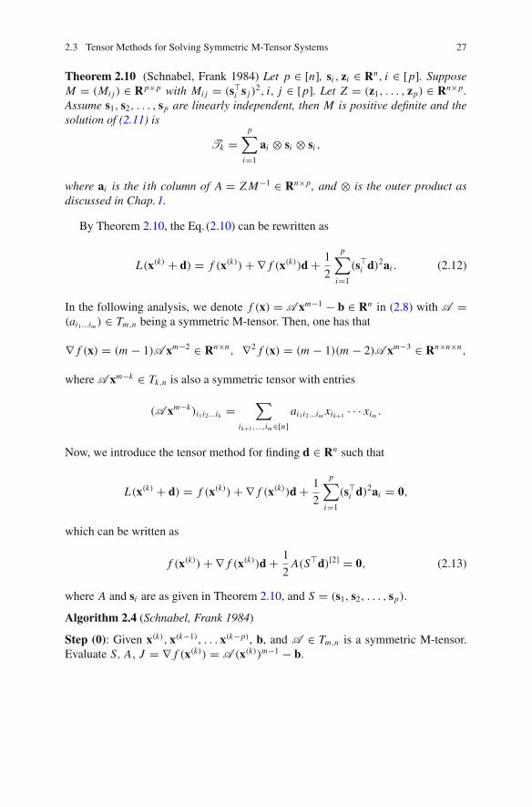
Theorem 2.10 (Schnabel, Frank 1984) Let p ∈ [n], si , zi ∈ Rn, i ∈ [p]. SupposeM = (Mi j ) ∈ Rp×p with Mi j = (s
i s j )2, i, j ∈ [p]. Let Z = (z1, . . . , zp) ∈ Rn×p.
Assume s1, s2, . . . , sp are linearly independent, then M is positive definite and thesolution of (2.11) is
Tk =p
∑
i=1
ai ⊗ si ⊗ si ,
where ai is the i th column of A = Z M−1 ∈ Rn×p, and ⊗ is the outer product asdiscussed in Chap.1.
By Theorem 2.10, the Eq. (2.10) can be rewritten as
L(x(k) + d) = f (x(k)) + ∇ f (x(k))d + 1
2
p∑
i=1
(s i d)2ai . (2.12)
In the following analysis, we denote f (x) = A xm−1 − b ∈ Rn in (2.8) with A =(ai1...im ) ∈ Tm,n being a symmetric M-tensor. Then, one has that
∇ f (x) = (m − 1)A xm−2 ∈ Rn×n, ∇2 f (x) = (m − 1)(m − 2)A xm−3 ∈ Rn×n×n,
where A xm−k ∈ Tk,n is also a symmetric tensor with entries
(A xm−k)i1i2...ik =∑
ik+1,...,im∈[n]ai1i2...im xik+1 · · · xim .
Now, we introduce the tensor method for finding d ∈ Rn such that
L(x(k) + d) = f (x(k)) + ∇ f (x(k))d + 1
2
p∑
i=1
(s i d)2ai = 0,
which can be written as
f (x(k)) + ∇ f (x(k))d + 1
2A(S d)[2] = 0, (2.13)
where A and si are as given in Theorem 2.10, and S = (s1, s2, . . . , sp).
Algorithm 2.4 (Schnabel, Frank 1984)
Step (0): Given x(k), x(k−1), . . . x(k−p), b, and A ∈ Tm,n is a symmetric M-tensor.Evaluate S, A, J = ∇ f (x(k)) = A (x(k))m−1 − b.

28 2 Multilinear Systems
Step (1): Find an orthogonal matrix Q ∈ Rn×n such that S = Q S, where
S =(
0S2
)
∈ Rn×n, S2 =
⎛
⎜
⎜
⎜
⎜
⎝
0 · · · 0 0 ∗0 · · · 0 ∗ ∗0 · · · ∗ ∗ ∗... . .
. ......
...
∗ · · · ∗ ∗ ∗
⎞
⎟
⎟
⎟
⎟
⎠
,
and S2 ∈ Rp×p is an anti-triangular matrix.
Step (2): Calculate J = J Q = (J1, J2) ∈ Rn×n , where J1 ∈ Rn×(n−p) and J2 ∈Rn×p are the first n − p and last p columns of J , respectively. Denote
d = Q d =(
d1d2
)
∈ Rn,
where d1 ∈ Rn−p and d2 ∈ Rp are the first n − p and last p components of J ,respectively.
Step (3): Find an orthogonal Q ∈ Rn×n and a permutation matrix P ∈ R(n−p)×(n−p)
such that
Q J1 P =
⎛
⎜
⎜
⎜
⎜
⎜
⎜
⎜
⎜
⎜
⎜
⎜
⎝
∗ ∗ ∗ · · · ∗ · · · ∗0 ∗ ∗ · · · ∗ · · · ∗0 0 ∗ · · · ∗ · · · ∗...
......
. . .... · · · ...
0 0 0 · · · ∗ · · · ∗0 0 0 · · · 0 · · · 0...
...... · · · ... · · · ...
0 0 0 · · · 0 · · · 0
⎞
⎟
⎟
⎟
⎟
⎟
⎟
⎟
⎟
⎟
⎟
⎟
⎠
=(
˜J1
0
)
∈ Rn×(n−p),
where the number of zero rows is q ≥ p, and ˜J1 ∈ R(n−q)×(n−p) is in echelon formwith a nonzero diagonal. Define ˜d1 = P
d1 ∈ Rn−p.
Step (4): Calculate
Q J2 =(
˜J2˜J3
)
, ˜A = ˜Q A =(
˜A1˜A2
)
, and ˜f = Q f =(
˜f1˜f2
)
,
where ˜J2, ˜A1 ∈ R(n−q)×p, ˜f1 ∈ Rn−q and ˜J3, ˜A2 ∈ Rq×p, ˜f2 ∈ Rq .
Step (5): Find a d2 such that
˜f2 + ˜J3 d2 + 1
2˜A2(S
2
d2)[2] = 0. (2.14)

2.3 Tensor Methods for Solving Symmetric M-Tensor Systems 29
Furthermore, we can solve it in the least squares sense which is
mind2∈Rp
‖ ˜f2 + ˜J3d2 + 1
2˜A2(S
2
d2)[2]‖2,
since the above quadratic equations (2.14) may have no solution.
Step (6): Find a ˜d1 such that
˜J1˜d1 = − ˜f1 − ˜J2d2 − 1
2˜A1(S
2
d2)[2].
Step (7): Calculate d1 = P˜d1, d = Qd.For Algorithm 2.4, it should be noted that Steps (1)-(2) aim to change the system
f + Jd + 1
2A(S d)[2] = 0
to another system
f + J1d1 + J2d2 + 1
2A(S
2d2)
[2] = 0,
which can be transformed to another system in Steps (3)-(4) such that
(
˜f1˜f2
)
+(
˜J1 ˜J2
0 ˜J3
)(
˜d1d2
)
+ 1
2
(
˜A1˜A2
)
(S 2
d2)[2] = 0.
Then the system above can also be transformed to the system with n − q equationsin n unknowns and the system with q equations in p unknowns such that
˜f1 + ˜J1˜d1 + ˜J2˜d2 + 1
2˜A1(S
2
d2)[2] = 0,
˜f2 + ˜J3˜d2 + 1
2˜A2(S
2
d2)[2] = 0.
After obtaining a solution d to the system (2.13), we give a framework for a fulltensor method.
Algorithm 2.5 (Schnabel, Frank 1984) Given x(k), x(k−1), . . . , x(k−p),A , b and tol.
Step 1: Evaluate fk = f (x(k)) and decide whether to stop, if not, go to Step 2.
Step 2: Evaluate Sk, Ak and Jk = ∇ f (x(k)).
Step 3: Find a solution dk to the tensor model (2.13) by Algorithm 2.4.
Step 4: Update x(k+1) = x(k) + dk, and go to Step 1.
30 2 Multilinear Systems
Next, based on the rank-1 approximation of the proposed tensor A , we introducea new tensor method for the system (2.2):
A xm−1 − b = 0.
Recall the results from [12, 61], for a symmetric tensor A ∈ Tm,n , we know that
A ≈p
∑
i=1
λi t(i) ⊗ t(i) ⊗ · · · ⊗ t(i),
where t(i) ∈ Rn are unit vectors i.e. ‖t(i)‖2 = 1. Hence, the second derivative ofA xm−1 is that
∇2 f (x) =(m − 1)(m − 2)A xm−3
≈(m − 1)(m − 2)(
p∑
i=1
λi t(i) ⊗ t(i) ⊗ · · · ⊗ t(i))xm−3
=(m − 1)(m − 2)
[
p∑
i=1
λi ((t(i)) x)m−3(t(i) ⊗ t(i) ⊗ t(i))
]
.
Hence, the tensor model (2.10) can be written as
L(x(k) + d) = f (x(k)) + ∇ f (x(k))d
+ 1
2(m − 1)(m − 2)
[
p∑
i=1
λi ((t(i)) x)m−3((t(i)) d)2t(i)
]
.(2.15)
Then, for solving the tensor system A xm−1 − b with A being a symmetric M-tensor,we have the following algorithm.
Algorithm 2.6 Given x(k), x(k−1), . . . , x(k−p),A , b and tol. Compute λi and t(i) suchthat
A ≈p
∑
i=1
λi t(i) ⊗ t(i) ⊗ · · · ⊗ t(i).
Step 1: Evaluate fk = f (x(k)) and decide whether to stop, if not, go to Step 2.
Step 2: Compute Jk = ∇ f (x(k)).
Step 3: Find a solution dk to the tensor model (2.15) according to Algorithm2.4 by setting Sk = (t(1), t(2), . . . , t(p)) and Ak = (a(k)
1 , a(k)2 , . . . , a(k)
p ), where a(k)i =
(m − 1)(m − 2)λi ((t(i)) x)m−3t(i).
Step 4: Update x(k+1) = x(k) + dk , and go to Step 1.

2.3 Tensor Methods for Solving Symmetric M-Tensor Systems 31
To prove the convergence of the new tensor method, we first present severallemmas, which will be used in the following analysis.
Lemma 2.2 For any A = (ai1i2...im ) ∈ Tm,n and x ∈ Rn, it holds that(1) ‖A x‖F ≤ ‖A ‖F‖x‖2;(2) ‖A xk‖F ≤ ‖A ‖F‖x‖k
2, where 1 ≤ k ≤ m.
Proof By the notion of Frobenius norm and Cauchy–Schwarz inequality, it followsthat
‖A x‖2F =
n∑
i1,...,im−1=1
|n
∑
im=1
ai1i2...im xim |2
≤n
∑
i1,...,im−1=1
⎛
⎝
n∑
im=1
|ai1i2...im |2⎞
⎠
⎛
⎝
n∑
im=1
|xim |2⎞
⎠
=‖A ‖2F‖x‖2
2.
Hence, we have ‖A x‖F ≤ ‖A ‖F‖x‖2.On the other hand, since A xk = (A xk−1)x, it follows from (1) that
‖A xk‖F =‖(A xk−1)x‖F ≤ ‖A xk−1‖F‖x‖2
=‖(A xk−2)x‖F‖x‖2 ≤ ‖A xk−2‖F‖x‖22
=‖(A xk−3)x‖F‖x‖22 ≤ · · · ≤ ‖A ‖F‖x‖k
2,
which implies the desired result holds. �
From Lemma 2.2, we have the following results.
Lemma 2.3 Suppose A ∈ T3,n and x, y ∈ Rn. Then
‖A x2 − A y2‖2 ≤ ‖A ‖F (‖x‖2 + ‖y‖2)‖x − y‖2.
Proof By Lemma 2.2, we have
‖A x − A y‖F = ‖A (x − y)‖F ≤ ‖A ‖F‖x − y‖2.
Then we obtain that
‖A x2 − A y2‖2 =‖(A x)x − (A y)x + (A y)x − (A y)y‖2
≤‖(A x − A y)x‖2 + ‖A y(x − y)‖2
≤‖A x − A y‖F‖x‖2 + ‖A y‖F‖x − y‖2
≤‖A ‖F‖x − y‖2‖x‖2 + ‖A ‖F‖x − y‖2‖y‖2
=‖A ‖F (‖x‖2 + ‖y‖2)‖x − y‖2,
and the desired result holds. �
32 2 Multilinear Systems
Combining Lemma 2.2 with the fact that f (x) = A xm−1 − b is continuous dif-ferentiable, we have the following results.
Lemma 2.4 (Xie, Jin, Wei 2017) For the system f (x) = A xm−1 − b = 0, assumeit has a solution x∗ and ∇ f (x) ∈ Rn×n is nonsingular in a neighborhood Ω of x∗.Then there exist scalars ε > 0, K > 0 and Mk > 0, k ∈ [m − 1] such that
‖(∇ f (x))−1‖F ≤ K , ‖∇k f (x)‖F ≤ Mk
for all ‖x − x∗‖2 ≤ ε, where ∇k f (x) is the kth derivative of f (x).
Now we show the local convergence of the tensor method under reasonable con-ditions.
Theorem 2.11 Assume dk = x(k+1) − x(k) obtained from Algorithm 2.6 satisfies
f (x(k)) + ∇ f (x(k))dk + 1
2∇2 f (x(k))(dk)
2 = Ek(dk)3, (2.16)
where Ek is a fourth order tensor with ‖Ek‖F being bounded. Suppose the sequence{x(k)} generated from Algorithm 2.6 converges to x∗, which is the roof of the equationf (x) = A xm−1 − b = 0. Suppose ∇ f (x) ∈ Rn×n is nonsingular in a neighborhoodΩ of x∗. Then there is a constant C such that
‖x(k+1) − x∗‖2 � C‖x(k) − x∗‖32.
Proof By the Taylor expansion, we know that
f (x∗) = f (x(k)) + ∇ f (x(k))(x∗ − x(k)) + 1
2∇2 f (x(k))(x∗ − x(k))2
+ 1
6∇3 f (ξ (k))(x∗ − x(k))3. (2.17)
Since f (x∗) = 0 and ∇ f (x) is nonsingular, (2.17) becomes
−(∇ f (x(k)))−1 f (x(k)) =(x∗ − x(k)) + 1
2(∇ f (x(k)))−1[∇2 f (x(k))(x∗ − x(k))2]
+ 1
6(∇ f (x(k)))−1[∇3 f (ξ (k))(x∗ − x(k))3].
By (2.16) it holds that
−(∇ f (x(k)))−1 f (x(k)) =(x(k+1) − x(k)) + 1
2(∇ f (x(k)))−1[∇2 f (x(k))(x(k+1) − x(k))2]
− (∇ f (x(k)))−1[Ek(x(k+1) − x(k))2].

2.3 Tensor Methods for Solving Symmetric M-Tensor Systems 33
Based on the above equation, we further have that
(x∗ − x(k)) + 1
2(∇ f (x(k)))−1[∇2 f (x(k))(x∗ − x(k))2]
+ 1
6(∇ f (x(k)))−1[∇3 f (ξ (k))(x∗ − x(k))3]
= xk+1 − x(k) + 1
2(∇ f (x(k)))−1[∇2 f (x(k))(x(k+1) − x(k))2]
− (∇ f (x(k)))−1[Ek(x(k+1) − x(k))3],
which implies that
x(k+1) − x∗ =1
2(∇ f (x(k)))−1[∇2 f (x(k))(x∗ − x(k))2]
− 1
2(∇ f (x(k)))−1[∇2 f (x(k))(x(k+1) − x(k))2]
+ 1
6(∇ f (x(k)))−1[∇3 f (ξ (k))(x∗ − x(k))3]
+ (∇ f (x(k)))−1[Ek(x(k+1) − x(k))3].
Taking the Euclidean norm on both sides, we get
‖x(k+1) − x∗‖2 ≤‖1
2(∇ f (x(k)))−1[∇2 f (x(k))(x∗ − x(k))2]
− 1
2(∇ f (x(k)))−1[∇2 f (x(k))(x(k+1) − x(k))2]‖2
+ ‖1
6(∇ f (x(k)))−1[∇3 f (ξ (k))(x∗ − x(k))3]‖2
+ ‖(∇ f (x(k)))−1[Ek(x(k+1) − x(k))3]‖2.
(2.18)
On the other hand, recall the notion of mode-1 tensor-matrix product in Chap. 1, thenwe have
(∇ f (x(k)))−1[∇2 f (x(k))(x∗ − x(k))2] = [∇2 f (x(k)) ×1 (∇ f (x(k)))−1](x∗ − x(k))2.
By Lemma 2.3, one obtains that
‖(∇ f (x(k)))−1[∇2 f (x(k))(x∗ − x(k))2] − 1
2(∇ f (x(k)))−1[∇2 f (x(k))(x(k+1) − x(k))2]‖2
= 1
2‖[∇2 f (x(k)) ×1 (∇ f (x(k)))−1](x∗ − x(k))2 − [∇2 f (x(k)) ×1 (∇ f (x(k)))−1](x(k+1) − x(k))2‖2
≤ 1
2‖∇2 f (x(k)) ×1 (∇ f (x(k)))−1‖F (‖x∗ − x(k)‖2 + ‖x(k+1) − x(k)‖2)‖x(k+1) − x∗‖2.
34 2 Multilinear Systems
Therefore, from (2.18), it holds that
‖x(k+1) − x∗‖2 ≤ 1
2‖∇2 f (x(k)) ×1 (∇ f (x(k)))−1‖F (‖x∗ − x(k)‖2 + ‖x(k+1) − x(k)‖2)‖x(k+1) − x∗‖2
+ 1
6‖∇3 f (ξ (k)) ×1 (∇ f (x(k)))−1‖F ‖x(k) − x∗‖3
2
+ ‖Ek×1(∇ f (x(k)))−1‖F ‖x(k+1) − x(k)‖32
≤ 1
2‖∇2 f (x(k))‖F ‖(∇ f (x(k)))−1‖F (‖x∗ − x(k)‖2 + ‖x(k+1) − x(k)‖2)‖x(k+1) − x∗‖2
+ 1
6‖∇3 f (ξ (k))‖F ‖(∇ f (x(k)))−1‖F ‖x(k) − x∗‖3
2
+ ‖Ek‖F ‖(∇ f (x(k)))−1‖F ‖x(k+1) − x(k)‖32.
(2.19)It is obvious that ‖x(k) − x∗‖2 → 0, ‖x(k+1) − x(k)‖2 → 0 as k → ∞ since x(k) →x∗. And we further have
1
2‖∇2 f (x(k))‖F‖(∇ f (x(k)))−1‖F (‖x∗ − x(k)‖2 + ‖x(k+1) − x(k)‖2) ≤ 1
2.
Then we get that
‖x(k+1) − x(k)‖32 =‖x(k+1) − x∗ + x∗ − x(k)‖2
2
≤(‖x(k+1) − x∗‖2 + ‖x(k) − x∗‖2)3
≈8‖x(k) − x∗‖32.
By (2.19), one has that
‖x(k+1) − x∗‖2 �(
1
3‖∇3 f (ξ (k))‖F + 16‖Ek‖F
)
‖(∇ f (x(k)))−1‖F‖x(k) − x∗‖32.
Let k → ∞ in the right side of the equation above, it follows that
(
1
3‖∇3 f (x∗)‖F + 16‖Ek‖F
)
‖(∇ f (x∗))−1‖F . (2.20)
By Lemma 2.4 and the fact that ‖Ek‖F is bounded, we can always take a constantC which is larger than the value in (2.20). Then we know that ‖x(k+1) − x∗‖2 �C‖x(k) − x∗‖3
2 and the desired results hold. �
It was noted by Xie et al. in [291] that the tensor method has a faster localconvergence rate than the classical Newton method.
2.4 Solution Methods for General Multilinear Systems 35
2.4 Solution Methods for General Multilinear Systems
In previous sections, we studied M-tensor equation systems with symmetricM-tensors and nonsymmetric M-tensors. In this section, we study solution meth-ods for a general multilinear system
A xm−1 = b. (2.21)
The methods studied in this section include Jacobi, the Gauss–Seidel and the suc-cessive over-relaxation (SOR) methods. The content of this section is based upon Liet al. in [168].
To move on, we need the following concepts. The diagonal tensors and triangulartensors defined here have a different version with previous sections.
Definition 2.1 A tensor D = (di1i2...im ) ∈ Tm,n is called a diagonal face tensor if itsentries satisfy
di1i2...im = 0, if i2 �= i1.
A tensor L = (li1i2...im ) ∈ Tm,n is called a lower half tensor if its entries satisfy
li1i2...im = 0, if i2 > i1,
It is called a strictly lower half tensor if
li1i2...im = 0, if i2 ≥ i1.
We may define upper half tensors and strictly upper half tensors similarly.
Suppose that D , L and L ′ are the diagonal face, lower half and strictly lowerhalf parts of a tensor A , respectively. Then we have the following observations:(1) If A is symmetric, then its diagonal face part D is also symmetric;(2) The numbers of entries of a (strictly) lower half tensor and an (strictly) upper halftensor are equal;(3) For any x ∈ Rn , Dxm−2, L xm−2 and L ′xm−2 are the diagonal, lower and strictlylower triangle parts of A xm−2, respectively. In particular, for any x ∈ Rn , we have
Dxm−2 = diag(A xm−2),
L xm−2 =
⎛
⎜
⎜
⎝
A11xm−2 0 · · · 0A21xm−2 A22xm−2 · · · 0
......
. . . 0An1xm−2 An2xm−2 · · · Annxm−2
⎞
⎟
⎟
⎠
36 2 Multilinear Systems
and
L ′xm−2 =
⎛
⎜
⎜
⎝
0 0 · · · 0A21xm−2 0 · · · 0
......
. . . 0An1xm−2 An2xm−2 · · · 0
⎞
⎟
⎟
⎠
,
where Ai j = (ai ji3i4...im )ni3,...,im=1, i, j = 1, 2, . . . , n.
For any nonsingular matrix E ∈ Rn×n and any nonzero scalar α, we see that xis a solution of the multilinear system A xm−1 − b = 0 if and only if it solves thefollowing fixed point problem
x = (
I + αE−1A xm−2)
x − αE−1b.
According to this, we set the following iterative scheme:
x(k+1) =(
I + αk E−1k A
(
x(k))m−2
)
x(k) − αk E−1k b. (2.22)
When m = 2, the iterative scheme (2.22) is an iterative method for solving thesystem of linear equations, with a fixed iterative matrix. If m ≥ 3, the iterative matrixI + αk E−1
k A (x(k))m−2 is nonlinear with respect to x(k). However, we may still provethe following convergence theorem in a way similar to the case m = 2, such as in[269].
Theorem 2.12 Suppose that the sequence {x(k)} is generated by the iterative scheme(2.22). If there are constants ρ ∈ (0, 1) and M > 0 such that
σ(
I + αk E−1k A
(
x(k))m−2
)
≤ ρ, |αk |‖E−1k b‖ ≤ M,
then the iterative sequence {x(k)} converges to a solution of the multilinear system(2.21), where σ(A) denotes the spectral radius of matrix A.
The choice of matrix Ek in the iterative scheme (2.22) plays a central role in thisiterative method for solving multilinear system (2.21). For solving a system of linearequations, typical choices of matrix Ek include the diagonal part, the lower trianglepart of the coefficient matrix, or some appropriate lower triangle matrix, correspond-ing to the Jacobi, the Gauss–Seidel or the successive over-relaxation (SOR) method.This idea was recently extended to solve multilinear system (2.21) [168].
Let A ∈ Sm,n . Then the multilinear system (2.21) is the first order necessarycondition of the minimization problem
min f (x) = 1
mA xm − b x. (2.23)

2.4 Solution Methods for General Multilinear Systems 37
Split A to A = M − U . We have
f (x) = 1
mM xm − 1
mU xm − b x.
Li, Xie and Xu [168] approximate the first term of f (x) by a quadratic functionand the second term by a linear function. Then there is the following approximateproblem
min f(
x(k)) =1
2(m − 1)
(
x − x(k))
M(
x(k))m−2 (
x − x(k))
+ (
x − x(k)) (
M(
x(k))m−1 − U (x(k))m−1 − b
)
=1
2(m − 1)
(
x − x(k))
M(
x(k))m−2 (
x − x(k))
+ (
x − x(k)) (
A(
x(k))m−1 − b
)
.
Denote the solution of this approximate problem by x(k+1). We have
x(k+1) =x(k) − 1
m − 1
(
M(
x(k))m−2
)−1 (
A(
x(k))m−1 − b
)
=(
I − 1
m − 1
(
M(
x(k))m−2
)−1
A(
x(k))m−1
)
x(k) + 1
m − 1
(
M(
x(k))m−2
)−1
b
=Hkx(k) + bk ,
(2.24)where
Hk = I − 1
m − 1
(
M(
x(k))m−2
)−1A
(
x(k))m−1
, bk = 1
m − 1
(
M(
x(k))m−2
)−1b.
By Theorem 2.12, a sufficient condition for the convergence of the iterative schemeis that there are constants ρ ∈ (0, 1) and C > 0 such that
σ(Hk) ≤ ρ, and ‖bk‖ ≤ C.
In (2.24), setting M = D, the diagonal face part of A , we have the Jacobimethod, which is an extension of the Jacobi method for solving the system of linearequations. Similarly, setting M = L , the lower half part of A , we have the Gauss–Seidel method. And setting M = 1
ω(D + ωL ′), we have the SOR method, where ω
is a relaxation parameter. We may write the Jacobi, Gauss–Seidel, and SOR methodsas follows:

38 2 Multilinear Systems
• The Jacobi method
x(k+1) = x(k) − 1
m − 1
(
D(
x(k))m−2
)−1 (
A(
x(k))m−1 − b
)
, k = 0, 1, . . . .
• The Gauss–Seidel method
x(k+1) = x(k) − 1
m − 1
(
L(
x(k))m−2
)−1 (
A(
x(k))m−1 − b
)
, k = 0, 1, . . . .
• The SOR method
x(k+1) = x(k) − ω
m − 1
(
(
D + ωL ′) (
x(k))m−2
)−1 (
A(
x(k))m−1 − b
)
, k = 0, 1, . . . .
We may also write the above iterative methods in the form (2.22) corresponding toαk = −1
m−1 ,
Ek = D(
x(k))m−2
, L(
x(k))m−2
and1
ω(D + ωL ′)
(
x(k))m−2
,
respectively. Then the Gauss–Seidel method is an SOR method that corresponds toω = 1.
Theorem 2.13 Let A ∈ Sm,n and x∗ be a solution of the tensor equation (2.21) suchthat A (x∗)m−2 is positive definite. Then the following statements hold.(1) There is a neighborhood U (x∗) of x∗ such that, as long as x0 ∈ U (x∗), thesequence {x(k)} generated by the Gauss–Seidel method converges to x∗.(2) If the matrix 2D(x∗)m−2 − A (x∗)m−2 is positive definite, then there is a neigh-borhood U (x∗) of x∗ such that, as long as x0 ∈ U (x∗), the sequence {x(k)} generatedby the Jacobi method converges to x∗.(3) If 0 < ω < 2, then there is a neighborhood U (x∗) of x∗ such that, as long asx0 ∈ U (x∗), the sequence {x(k)} generated by the SOR method converges to x∗.In either case, the convergence rate of {x(k)} is at least r-linear.
Proof We only prove the convergence of the SOR method. As discussed above,the Gauss–Seidel method is a special case of the SOR method when ω = 1. Theconvergence of the Jacobi method can be proved similarly. Let
Lk(ω) = (D + ωL ′)(
x(k))m−2 = (1 − ω)D
(
x(k))m−2 + ωL
(
x(k))m−2
and
dk = − ω
m − 1Lk(ω)−1
(
A(
x(k))m−1 − b
)
= − ω
m − 1Lk(ω)−1∇ f
(
x(k))
.

2.4 Solution Methods for General Multilinear Systems 39
We may write the SOR method as x(k+1) = x(k) + dk . By the definition of D and L ,we have the following equality,
p Lk(ω)p = 1
2ωp
(
A(
x(k))m−2
)
p +(
1 − 1
2ω
)
p (
D(
x(k))m−2
)
p > 0, ∀ p ∈ Rn .
(2.25)Since f (x) = 1
m A xm − b x, by Taylor’s expansion, we have
f (x(k+1)) = f (x(k)) + d k ∇ f (x(k)) + 1
2(m − 1)d
k ∇2 f (x(k))dk
= f (x(k)) − 1
ω(m − 1)d
k Lk(ω)dk + 1
2(m − 1)d
k (A (x(k))m−2)dk
= f (x(k)) − (m − 1)
(
1
ωd
k Lk(ω)dk − 1
2d
k (A (x(k))m−2)dk
)
+ m − 1
2d
k εkdk
= f (x(k)) − 1
ω
(
1 − 1
2ω
)
(m − 1)d k (D(x(k))m−2)dk + m − 1
2d
k εkdk ,
wherex(k) = x(k) + θk(x(k+1) − x(k))
with θk ∈ (0, 1) and εk = A (x(k))m−2 − A (x(k))m−2 tends to zero if x(k) converges.We may show by induction that
{d k D(x(k))m−2dk} → 0, and {dk} → 0,
or equivalentlylim
k→∞(L (x(k))m−2)−1(A (x(k))m−1 − b) = 0.
This, combined with the fact thatL (x∗)m−2 is positive definite, impliesA (x(k))m−1 −b → 0.
Since D(x∗)m−2 is positive definite, the convergence rate of {x(k)} is at least r -linear. The theorem is proved. �
In the remainder of this section, we will globalize the method. We only globalizethe Gauss–Seidel method. The Jacobi and SOR methods can be globalized similarly.We assume that for any x �= 0 the matrix A xm−2 is positive semidefinite with positivediagonals.
We rewrite the Gauss–Seidel method as
x(k+1) = x(k) + dk,
where dk is the solution of the system of linear equations
(m − 1)Lkd + ∇ f (x(k)) = 0, (2.26)

40 2 Multilinear Systems
f is defined by (2.23) and Lk = L (x(k))m−2. Since A (x(k))m−2 is positive semidef-inite with positive diagonals, by (2.25) with ω = 1, we have
d k Lkdk ≥ 1
2d
k (D(x(k))m−2dk > 0, (2.27)
which further implies
∇ f (x(k)) dk = −(m − 1)d k Lkdk < 0.
This indicates that the Gauss–Seidel direction is a descent direction of the objectivefunction. Then we may globalize the method by using a line search process. Thisresults in the following damped Gauss–Seidel method,
x(k+1) = x(k) + αkdk,
where dk is the Gauss–Seidel direction and the steplength αk is obtained by someline search process such as the Armijo or the Wolfe line search process.
The Armijo line search finds a steplength αk = ρi with ρi ∈ (0, 1), where i is thesmallest positive integer such that
f (x(k) + ρi dk) ≤ f (x(k)) + σ1ρi∇ f (x(k)) dk, (2.28)
where σ1 ∈ (0, 1). The Wolfe line search finds a steplength αk such that
{
f (x(k) + αkdk) ≤ f (x(k)) + σ1αk∇ f (x(k)) dk,
∇ f (x(k) + αkdk) dk ≥ σ2∇ f (x(k)) dk,
(2.29)
where 0 < σ1 < σ2 < 1.
Theorem 2.14 Suppose that for any x �= 0, the matrix A xm−2 is positive semidefi-nite. Then every accumulation point of the sequence {x(k)} generated by the dampedGauss–Seidel method with Armijo or Wolfe line search is a solution of the minimiza-tion problem (2.23).
Proof Since the matrix A xm−2 is positive semidefinite for any x �= 0, f is convex.For a continuously differentiable convex function, every stationary point is a globalminimizer. Hence, it suffices to prove that every accumulation point of {x(k)} is astationary point of the problem.
Suppose that x∗ is an arbitrary accumulation point of {x(k)}. That is to say, thereexists a subsequence {x(k) : k ∈ K } that converges to x∗. By (2.26) and (2.27), thereare constants C2 ≥ C1 > 0 such that the inequalities
C1‖∇ f (x(k))‖ ≤ ‖dk‖ ≤ C2‖∇ f (x(k))‖ (2.30)
2.4 Solution Methods for General Multilinear Systems 41
hold for all sufficiently large k ∈ K . In particular, the sequence {‖dk‖} is bounded.Without loss of generality, assume that {dk : k ∈ K }K converges to some d∗. Lettingk → ∞ in (2.26) with k ∈ K , we have
(m − 1)L (x∗)m−2d∗ + ∇ f (x∗) = 0. (2.31)
By (2.28) or the first condition in (2.29), we also have
limk→∞ αk∇ f (x(k)) dk → 0.
In the case where Armijo line search is used, if lim supk∈K αk > 0, then we have
limk→∞ ∇ f (x(k)) dk → 0.
This combined with (2.31) indicates ∇ f (x∗) = 0. If lim infk∈K αk = 0, then whenk is sufficiently large, we have
f (x(k) + αkρ−1dk) − f (x(k)) > σ1αkρ
−1∇ f (x(k)) dk .
Multiplying both sides of the last inequality by α−1k ρ and letting k → ∞ with k ∈ K ,
we have∇ f (x∗) d∗ ≥ 0.
This combined with (2.31) again indicates ∇ f (x∗) = 0, i.e., x∗ is a stationary pointof the problem.
In the case that Wolfe line search is used, let θk be the angle between −∇ f (x(k))
and dk . By the Zoutendijk condition
∞∑
k=0
‖∇ f (x(k))‖2 cos2 θk < ∞,
we only need to prove that {cos θk}K is bounded away from zero. In fact, we have
cos θk = −∇ f (x(k)) dk
‖∇ f (x(k))‖‖dk‖ = (m − 1)d k Lkdk
‖∇ f (x(k))‖‖dk‖ ≥12 (m − 1)d
k Dkdk
C−11 ‖dk‖2
,
where the inequality follows from (2.27) and (2.30). Since {Dk}k∈K → D∗ is posi-tive definite, the last inequality indicates that there exists a constant δ > 0 such thatcos θk ≥ δ for all sufficiently large k ∈ K . Hence, we have limk→∞,k∈K ‖∇ f (x(k))‖ =0, i.e., x∗ is a stationary point of the problem. The theorem is proved. �
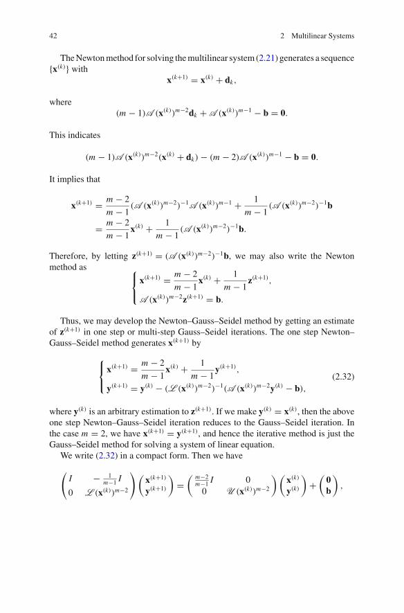
42 2 Multilinear Systems
The Newton method for solving the multilinear system (2.21) generates a sequence{x(k)} with
x(k+1) = x(k) + dk,
where(m − 1)A (x(k))m−2dk + A (x(k))m−1 − b = 0.
This indicates
(m − 1)A (x(k))m−2(x(k) + dk) − (m − 2)A (x(k))m−1 − b = 0.
It implies that
x(k+1) = m − 2
m − 1(A (x(k))m−2)−1A (x(k))m−1 + 1
m − 1(A (x(k))m−2)−1b
= m − 2
m − 1x(k) + 1
m − 1(A (x(k))m−2)−1b.
Therefore, by letting z(k+1) = (A (x(k))m−2)−1b, we may also write the Newtonmethod as
⎧
⎨
⎩
x(k+1) = m − 2
m − 1x(k) + 1
m − 1z(k+1),
A (x(k))m−2z(k+1) = b.
Thus, we may develop the Newton–Gauss–Seidel method by getting an estimateof z(k+1) in one step or multi-step Gauss–Seidel iterations. The one step Newton–Gauss–Seidel method generates x(k+1) by
⎧
⎨
⎩
x(k+1) = m − 2
m − 1x(k) + 1
m − 1y(k+1),
y(k+1) = y(k) − (L (x(k))m−2)−1(A (x(k))m−2y(k) − b),
(2.32)
where y(k) is an arbitrary estimation to z(k+1). If we make y(k) = x(k), then the aboveone step Newton–Gauss–Seidel iteration reduces to the Gauss–Seidel iteration. Inthe case m = 2, we have x(k+1) = y(k+1), and hence the iterative method is just theGauss–Seidel method for solving a system of linear equation.
We write (2.32) in a compact form. Then we have
(
I − 1m−1 I
0 L (x(k))m−2
)
(
x(k+1)
y(k+1)
)
=( m−2
m−1 I 00 U (x(k))m−2
) (
x(k)
y(k)
)
+(
0b
)
,

2.4 Solution Methods for General Multilinear Systems 43
where U = L − A . This implies
(
x(k+1)
y(k+1)
)
=(
I − 1m−1 I
0 L (x(k))m−2
)−1 ( m−2m−1 I 0
0 U (x(k))m−2
)(
x(k)
y(k)
)
+(
I − 1m−1 I
0 L (x(k))m−2
)−1 (
0b
)
=( m−2
m−1 I 1m−1 (L (x(k))m−2)−1U (x(k))m−2
0 (L (x(k))m−2)−1U (x(k))m−2
) (
x(k)
y(k)
)
+( 1
m−1 (L (x(k))m−2)−1b(L (x(k))m−2)−1b
)
=Bk
(
x(k)
y(k)
)
+ bk,
where
Bk =( m−2
m−1 I 1m−1 (L (x(k))m−2)−1U (x(k))m−2
0 (L (x(k))m−2)−1U (x(k))m−2
)
=I −( 1
m−1 I 1m−1 (L (x(k))m−2)−1U (x(k))m−2
0 (L (x(k))m−2)−1A (x(k))m−2
)
,
and
bk =( 1
m−1 (L (x(k))m−2)−1b(L (x(k))m−2)−1b
)
.
Since the matrix Bk is block upper triangular, its eigenvalues are m−2m−1 together
with eigenvalues of the Gauss–Seidel matrix (L (x(k))m−2)−1U (x(k))m−2. Thus, theconvergence of the iterative scheme is the same as the one of the Gauss–Seidelmethod.
Note that we may also use multi-step Gauss–Seidel steps to obtain an approximateNewton direction. Then we have the following iterative scheme:
⎧
⎨
⎩
x(k+1) = m − 2
m − 1x(k) + 1
m − 1y(k+1)
y(k+ j) = y(k+ j−1) − (L (x(k))m−2)−1(A (x(k))m−2y(k+ j−1) − b), j = 1, 2, . . . , i.
Li et al. [168] presented several numerical experiments to show that the multistepNewton–Gauss–Seidel method works quite well.

44 2 Multilinear Systems
2.5 Notes
The multilinear nonsingular M-equations and some extensions have been inves-tigated carefully in this chapter. Some well-known iterative methods for solvingsystem of linear equations are extended to the tensor equations. Under reasonableconditions, the convergence of the proposed methods are established. Furthermore,a Newton–Gauss–Seidel method, a homotopy method and a new tensor method arealso proposed for solving the M-tensor equation system.
Section 2.1 Conclusions in this section were first presented by Ding and Wei in[87]. M-tensors are Z-tensors, which was defined by Zhang, Qi, and Zhou in [305].Then, Z-tensors and M-tensors were further studied by Ding, Qi, and Wei in [82].H-matrices were extended to H-tensors in [82]. Section 5.4 of [228] was devoted toM-tensors and H-tensors, and the bibliography of [228] includes up-to-date refer-ences on applications of Z-tensors, M-tensors and H-tensors.
Section 2.2 Several numerical methods are studied in this section. The forwardsubstitution method and the back substitution method for multilinear systems withM-tensors were first proposed by Ding and Wei in [87]. Theorem 2.7 was citedfrom [234] by Rheinboldt. Another method for mulitilinear system is the homotopymethod, which was proposed by Han in [117].
Section 2.3 A tensor method for multilinear system is discussed in this section. Tosolve nonlinear equation systems, the tensor method was first introduced by Schnabeland Frank in [238]. Combining this idea with the results for the rank-1 approximationof tensors, Xie, Jin, and Wei proposed a new tensor method for solving the symmetricM-tensor equation system [291]. Theorem 2.10 and Algorithms 2.4–2.5 were provedby Schnabel, Frank in 1984 [238].
Section 2.4 In this part, several methods are studied for solving multilinear systemwith tensors with general structures. The methods include Jacobi, the Gauss–Seideland the successive over-relaxation (SOR) methods, which are well known basiciterative methods for solving system of linear equations. Here, they were extendedto solve the multilinear system by Li, Xie, and Xu in [168].
Besides above, there are some other results on tensor equation systems or havingclose relationships with tensor equation systems [25], which are different from theM-tensor equation system in this chapter. Now, we will describe the main idea of therelated papers in three parts.1. Li and Ng studied the sparse nonnegative tensor equation system in [170], wherethe related tensors Ak = (a(k)
i1i2...im), k ∈ [m] are nonnegative mth order n1 × n2 ×
· · · × nm dimensional stochastic tensors with respect to the kth dimension:
nk∑
ik=1
a(k)i1i2...im
= 1 for all il ∈ [nl], l ∈ [m], l �= k.
2.5 Notes 45
Here the tensor Ak may not be symmetric. Hence, the tensor equation model studiedin [170] is that
⎧
⎪
⎪
⎪
⎪
⎨
⎪
⎪
⎪
⎪
⎩
y(1) = (1 − α1)A1 ×1 y(2)y(3) · · · y(m) + α1z(1)
y(2) = (1 − α2)A2 ×2 y(1)y(3) · · · y(m) + α2z(2)
. . . . . . . . .
y(m) = (1 − αm)Am ×m y(1) · · · y(m−1) + αmz(m)
(2.33)
where z(k) ∈ Rnk are given nonnegative vectors such that∑nk
i=1 z(k)i = 1 for k ∈ [m]
and αk ∈ [0, 1] for k ∈ [m] are given scalars. It should be noted that the system(2.33) has a strong practical background such as community discovery for onlinesocial media, and information retrieval that can assist in many data mining tasks.
First of all, Li and Ng proved that there always exist solutions y(1), y(2), . . . , y(m)
satisfying (2.33) withnk
∑
i=1
y(k)i = 1, ∀k ∈ [m],
and furthermore, the solution vectors y(k), k ∈ [m] are positive vectors if the relatedtensors Ak, k ∈ [m] are irreducible. If suitable conditions are added to scalars αk
such thatm − 2
m − 1< αk < 1, ∀ k ∈ [m], (2.34)
then it is proved that the solutions y(k), k ∈ [m] of (2.33) are unique, and the resultsabove construct the main theoretical results in [170].
According to the main results listed above, Jacobi and Gauss–Seidel methodsare developed for solving tensor equation system (2.33). In the iterative process,the multiplication of tensors with vectors are required and the cost depends on thenumber of non-zeros in the tensors. Hence, the proposed Jacobi and Gauss–Seidelmethods are not expensive especially when the tensors are very sparse. Furthermore,the linear convergence of the Jacobi and Gauss–Seidel methods are established, andexperimental results on information retrieval by query search and community dis-covery in networks are also reported to demonstrate the effectiveness of the proposedmethods. Interested readers may check the details in [170].2. Since the polynomials corresponding to high order tensors have more complexstructures than polynomials corresponding to matrices, it is not easy to define theinverse like the matrix case. But it is possible to define generalized inverse of tensorsin some sense. With the help of the notion of tensor equation systems, Sun et al.[259] studied the {i}-inverse (i = 1; 2; 5) and group inverse of tensor A defined incomplex number field. Then, by the definition of {1}-inverse, some solutions for thetensor equation system
A xm−1 = b

46 2 Multilinear Systems
are given under reasonable conditions. It should be noted that all tensors and vectorsstudied in [259] are defined in complex number field C, and the definition of {i}-inverse for tensors is defined based on the tensor multiplication given by Shao in[240], which means that the multiplication A B of an order k dimension n tensor Aand an order t dimension n tensor B is a tensor with order k + t − 1 dimension n.
Now we give a short description for the main results of [259]. Suppose A is atensor with order t dimension m × n × · · · × n. If there is a tensor X with order kdimension n × m × · · · × m satisfying
A X (A ym−1)[1s ] = A yt−1, s = (t − 1)(k − 1),
for all vectors y ∈ Cn , then the tensor X is called a {1}-inverse of A with order k.It is not difficult to check that the {1}-inverse of tensors reduces to the {1}-inverse ofmatrices when A and X are matrices.
For tensor A given as above, if it has at least one {1}-inverse tensor X with orderk and the equation system A xt−1 = b is solvable, then it is proved by Sun et al.in [259] that the proposed equation system has a solution x = X (b[ 1
s ])k−1, wheres = (t − 1)(k − 1). By this, we know that one can get the solution of the systemdirectly if the {1}-inverse of the related coefficient tensor can be computed. Now, thequestion is how to compute the {1}-inverse tensor for a given tensor? The authorsof [259] did not present any methods to compute the {1}-inverse for a general giventensor. This may be an interesting work in the future.
However, for some tensors with special structure, we can obtain the {1}-inverseby a direct computation. For example, in [259], Sun et al. showed that, a diagonaltensor A ∈ Tm,n with diagonal entries a1, a2, . . . , an ∈ C has an k-order {1}-inversediagonal tensor with diagonal entries being (a†
1)1
t−1 , (a†2)
1t−1 , . . . , (a†
n)1
t−1 , where
a† ={
a−1, if a �= 00, if a = 0.
Furthermore, it shows how to characterize the representations for the {1}-inverse andgroup inverse of some block tensors [259], which extends the results on generalizedinverses of matrices. Since the results about block tensor are uncorrelated with thecontents of this chapter, we do not want to go far for the detail. Interested readersmay recall the related paper [259].3. Very recently, Liu et al. studied another kind of sparse nonnegative tensor systemsfor data sciences in [183], which can be seen as a further research for the paper[170]. For the tensor equation system (2.33), the uniqueness of solutions is provedunder conditions (2.34). However, in some practical problems, these parametersαk > 0, k ∈ [m] would tend to 1. Thus a question can be raised naturally: Can weexploit any better upper bounds for scalars αk? Motivated by this, Liu et al. devoted tostudy the uniqueness of solution for system (2.33), where explicit upper bounds forparameters αk are given [183]. In that paper, two different techniques are introducedto get better upper bound: the parameter method and the optimal set method.

2.5 Notes 47
On the other hand, with the two techniques, Liu et al. also considered the system(2.33) with a perturbation, which means the related stochastic tensors Ak, k ∈ [m]are replaced by Ak + �Ak, k ∈ [m] respectively. Here Ak + �Ak, k ∈ [m] are stillstochastic tensors. Then the authors presented a new perturbation tensor equationsystem, and studied the unique property of the solution of the new system, whichhas important applications in sensitivity analysis [183].
2.6 Exercise
1 Let A = I − B be a 3 × 3 × 3 singular M-tensor, where B is a nonnega-tive tensor with B12 = 1, and bi jk = 0 if i ∈ {2, 3} and either j = 1 or k = 1.Apparently, the subtensor A2:3,2:3,2:3 is also a singular M-tensor, which satisfies thatA2:3,2:3,2:312 = 0. For each right-hand side b = (b1, 0, 0), what is the form of thenonnegative solutions to A x2 = b?2 Suppose A ∈ T3,n is a third order symmetric M-tensor. Define A = sI − B,where B = (bi jk) with entries such that
bi jk = | sin(i + j + k)|.
Let s = n2. Prove A is a symmetric nonsingular M-tensor.
Chapter 3Hankel Tensor Computationand Exponential Data Fitting
Hankel structures are widely used in real-world problems arising from signal process-ing, automatic control, and geophysics. For example, a Hankel matrix was formulat-ed to analyze the time-domain signals in nuclear magnetic resonance spectroscopy,which is crucial for brain tumour detection [268]. Papy et al. [217, 218] improvedthis method by using a high order Hankel tensor to replace the Hankel matrix. Dinget al. [83] found a fast computational technique for computing products of a Hankeltensor and vectors.
Exploring the special structure, we first define two classes of tensors: Hankeltensors and anti-circulant tensors. They share the same generating vector. Second,we show that an anti-circulant tensor has a diagonal decomposition using fast Fouriertransforms. Then, we introduce the fast Hankel tensor–vector product.
For real-valued symmetric Hankel tensors, we propose an optimization approachfor computing extreme eigenvalues and associated eigenvectors. First, we considera spherical optimization problem, whose objective is a homogeneous polynomialinvolved in the Hankel tensor. The first-order stationary point of the optimizationproblem is an eigenvector of the tensor. Second, we propose a gradient-descentmethod for solving the spherical optimization, where the Cayley transform is usedto preserve the spherical constraint. Third, using the Łojasiewicz property of thehomogeneous polynomial involved in a tensor, we prove that the total sequence ofiterates generated by the gradient-descent method converges to an eigenvector andthe corresponding objective converges to the associated eigenvalue. When we startthe algorithm from plenty of randomly initial points sampled from the unit sphereuniformly, we could touch the extreme eigenvalue of the Hankel tensor with a higherprobability.
Finally, we study the application of Hankel tensors in exponential data fitting. Forsignals modeled as a sum of exponentially damped sinusoids, we arrange them asa Hankel tensor which has an inherent Vandermonde decomposition. The subspacespanned by the Vandermonde factor is approximated by the higher-order orthogonaliterations (HOOI). Here, the fast Hankel tensor–vector product accelerates HOOI
© Springer Nature Singapore Pte Ltd. 2018L. Qi et al., Tensor Eigenvalues and Their Applications, Advances in Mechanicsand Mathematics 39, https://doi.org/10.1007/978-981-10-8058-6_3
49
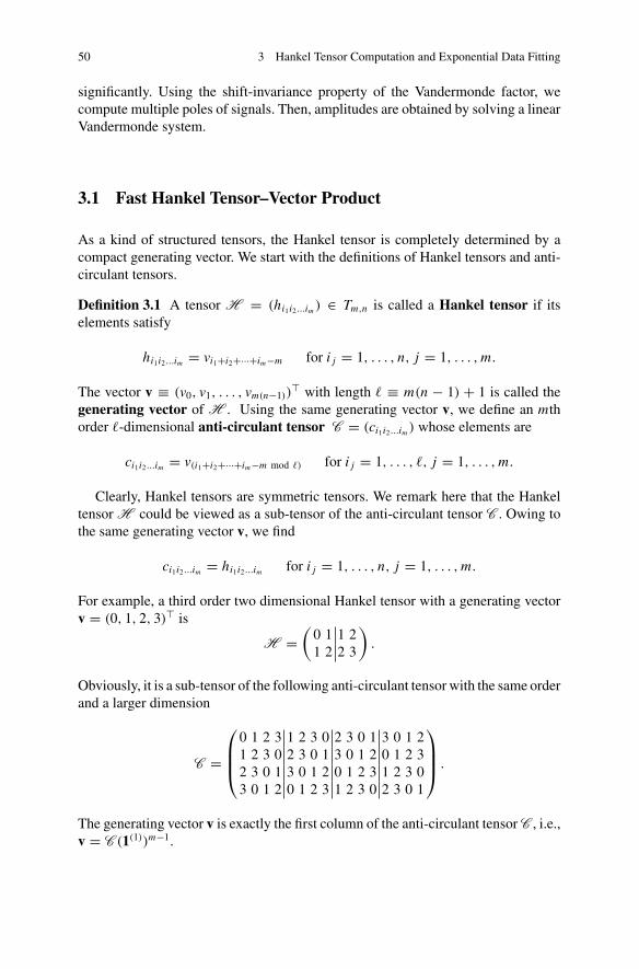
50 3 Hankel Tensor Computation and Exponential Data Fitting
significantly. Using the shift-invariance property of the Vandermonde factor, wecompute multiple poles of signals. Then, amplitudes are obtained by solving a linearVandermonde system.
3.1 Fast Hankel Tensor–Vector Product
As a kind of structured tensors, the Hankel tensor is completely determined by acompact generating vector. We start with the definitions of Hankel tensors and anti-circulant tensors.
Definition 3.1 A tensor H = (hi1i2...im ) ∈ Tm,n is called a Hankel tensor if itselements satisfy
hi1i2...im = vi1+i2+···+im−m for i j = 1, . . . , n, j = 1, . . . , m.
The vector v ≡ (v0, v1, . . . , vm(n−1))� with length � ≡ m(n − 1) + 1 is called the
generating vector of H . Using the same generating vector v, we define an mthorder �-dimensional anti-circulant tensor C = (ci1i2...im ) whose elements are
ci1i2...im = v(i1+i2+···+im−m mod �) for i j = 1, . . . , �, j = 1, . . . , m.
Clearly, Hankel tensors are symmetric tensors. We remark here that the Hankeltensor H could be viewed as a sub-tensor of the anti-circulant tensor C . Owing tothe same generating vector v, we find
ci1i2...im = hi1i2...im for i j = 1, . . . , n, j = 1, . . . , m.
For example, a third order two dimensional Hankel tensor with a generating vectorv = (0, 1, 2, 3)� is
H =(
0 1 1 21 2 2 3
).
Obviously, it is a sub-tensor of the following anti-circulant tensor with the same orderand a larger dimension
C =
⎛⎜⎜⎝
0 1 2 3 1 2 3 0 2 3 0 1 3 0 1 21 2 3 0 2 3 0 1 3 0 1 2 0 1 2 32 3 0 1 3 0 1 2 0 1 2 3 1 2 3 03 0 1 2 0 1 2 3 1 2 3 0 2 3 0 1
⎞⎟⎟⎠ .
The generating vector v is exactly the first column of the anti-circulant tensor C , i.e.,v = C (1(1))m−1.

3.1 Fast Hankel Tensor–Vector Product 51
The anti-circulant tensor enjoys a diagonalization via the Fourier matrix. Letω ≡ exp(− 2π i
�) ∈ C be a primitive �th root of unity, where i is the imaginary unit.
An �-by-� Fourier matrix is defined as
F� = (ω jk) j,k=0,1,...,�−1.
Note that F� = F�� . By some calculation, we have
F H� F� = �I,
where (·)H means the conjugate transpose.For example, in the case of � = 4, we have ω = exp(− 2π i
4 ) = −i and
F4 =
⎛⎜⎜⎝
1 1 1 11 −i −1 i1 −1 1 −11 i −1 −i
⎞⎟⎟⎠ .
Next, we give the following theorem on anti-circulant tensors [83].
Theorem 3.1 A tensor C ∈ Tm,n is an anti-circulant tensor if and only if it can bediagonalized by the Fourier matrix, i.e.,
C = D Fm� ≡ D ×1 F� ×2 F� · · · ×m F�,
where D is a diagonal tensor with diagonal elements diag(D) = F−1� v and v =
C (1(1))m−1 is the generating vector of the anti-circulant tensor C .
Proof First, we prove thatD Fm� is an anti-circulant tensor. The (i1, . . . , im)th element
of D Fm� is
(D Fm� )i1...im = (D Fm
� ) ×1 1(i1) · · · ×m 1(im ) = D ×1 (F�1(i1)) · · · ×m (F�1(im ))
for indices i1, . . . , im = 1, 2, . . . , �. Let diag(D) = (d0, d1, . . . , d�−1)�. We get
(D Fm� )i1...im =
�−1∑j=0
d jωj (i1−1) · · · ω j (im−1)
=�−1∑j=0
d jωj (i1+···+im−m)
=�−1∑j=0
d jωj (i1+···+im−m mod �).
52 3 Hankel Tensor Computation and Exponential Data Fitting
Hence, D Fm� is an anti-circulant tensor with a generating vector
(∑�−1
j=0 d jωjk)k=0,...,�−1.
On the other hand, if diag(D) = F−1� v, by some calculations, we have
(D Fm� )i1...im = (F−1
� v)�(F�1(1+(i1+···+im−m mod �))) = v(i1+···+im−m mod �)
for i1, . . . , im = 1, 2, . . . , �. Since v is the generating vector of the anti-circulanttensor C , the theorem is valid. �
It is well-known that the fast Fourier transform fft and its inverse transformifft could be employed to compute products involving a Fourier matrix and itsinverse, respectively. The computational cost of an (inverse) Fourier matrix–vectorproduct is about O(� log �) multiplications, which is cheap when the dimension � islarge.
Now, we are going to show how to compute the Hankel tensor–vector productusing Theorem 3.1. The basic idea is to enlarge the Hankel tensor to an anti-circulanttensor. For a given vector x ∈ Rn , we define another vector y ∈ R� such that
y ≡(
x0�−n
),
where � = m(n − 1) + 1 and 0�−n is a zero vector with length � − n. Then, we have
H xm = C ym = D(F�y)m = ifft(v)�(fft(y)◦m
).
To obtain H xm−1, we first compute
C ym−1 = F�
(D(F�y)m−1
) = fft(ifft(v) ◦ (fft(y)◦(m−1))
).
Then, elements of the vector H xm−1 is the leading n elements of C ym−1. Here, ◦denotes the Hadamard product such that (A ◦ B)i j = Ai j Bi j if A and B have thesame size. Furthermore, we denote
A◦k = A ◦ · · · ◦ A︸ ︷︷ ︸k times
as the Hadamard product of k copies of A.Since the computations ofH xm andH xm−1 require 2 and 3fft/iffts, respec-
tively, the cost is about O(mn log(mn)) multiplications and hence cheap. Anotheradvantage of this approach is that we only need to store and work with the compactgenerating vector of the Hankel tensor.

3.2 Computing Eigenvalues of a Hankel Tensor 53
3.2 Computing Eigenvalues of a Hankel Tensor
We consider the generalized eigenvalue [33, 86] of a real-valued Hankel tensorH ∈ Sm,n defined with the following system:
H xm−1 = λBxm−1, (3.1)
where m is even, B ∈ Sm,n is a positive definite tensor. If there is a scalar λ ∈ R anda vector x ∈ Rn\{0} satisfying the above system, we call λ a generalized eigenvalueof H and x its associated generalized eigenvector. Particularly, λ is an H-eigenvalueof H and x is its associated H-eigenvector if B = I where I xm−1 = x[m−1][221]. If B is a tensor E ∈ Sm,n such that E xm−1 = ‖x‖m−2x, then λ is called aZ-eigenvalue of H and x
‖x‖ is its associated Z-eigenvector. Obviously, computationson these tensors such like B are straightforward.
To compute a generalized eigenvalue and its associated eigenvector, we consideran optimization model with a spherical constraint
min f (x) ≡ H xm
Bxms.t. ‖x‖ = 1. (3.2)
To keep variables x away from zero, we introduce the spherical constraint ‖x‖ = 1.Since the objective f (x) is zero-order homogeneous, we do not need to consider themultiplier of the spherical constraint (See Theorem 3.2). By some calculations, weget its gradient
g(x) = m
Bxm
(H xm−1 − H xm
BxmBxm−1
)(3.3)
and Hessian
H(x) = m(m − 1)H xm−2
Bxm− m(m − 1)H xmBxm−2 + m2(H xm−1 � Bxm−1)
(Bxm)2
+ m2H xm(Bxm−1 � Bxm−1)
(Bxm)3, (3.4)
where x � y ≡ xy� + yx�.The relationship between eigenvalues of a Hankel tensor and the spherical opti-
mization problem (3.2) is established via the following theorem.
Theorem 3.2 Let m be even and x∗ ∈ Sn−1 ≡ {x ∈ Rn | x�x = 1}. Then, x∗ isa first-order stationary point of f (x), i.e., g(x∗) = 0, if and only if there exists aλ∗ ∈ R such that (λ∗, x∗) satisfies (3.1). Indeed, λ∗ = f (x∗) is the H-eigenvalue(resp., Z-eigenvalue) and x∗ is the associated H-eigenvector (resp., Z-eigenvector) ifB = I (resp., B = E ).
Proof Since B is positive definite and x∗ belongs to a compact set Sn−1, Bxm∗ hasa finite upper bound. Thus, λ∗ = H xm∗
Bxm∗= f (x∗) and the theorem is valid. �
54 3 Hankel Tensor Computation and Exponential Data Fitting
Next, we construct a curvilinear search path on the sphere Sn−1 via the Cayleytransform [37, 105]. Suppose that the current iterate is xk ∈ Sn−1 and the nextiterate is xk+1. To preserve the spherical constraint x�
k+1xk+1 = x�k xk = 1, we try to
choose an orthogonal matrix Q ∈ Rn×n , whose eigenvalues do not contain −1, suchthat
xk+1 = Qxk . (3.5)
Using the Cayley transform, the matrix
Q = (I + W )−1(I − W ) (3.6)
is orthogonal if and only if W ∈ Rn×n is skew-symmetric. Now, our task is to selecta skew-symmetric matrix W such that g(xk)
�(xk+1 − xk) < 0. For simplicity, wetake
W = ab� − ba�, (3.7)
where a, b ∈ Rn are two undetermined vectors. From (3.5) and (3.6), we have
xk+1 − xk = −W (xk + xk+1).
Then, by (3.7), it yields that
g(xk)�(xk+1 − xk) = −[(g(xk)
�a)b� − (g(xk)�b)a�](xk + xk+1).
Since the objective f (·) in (3.2) is zero-order homogeneous, we have
x�k g(xk) = 0, (3.8)
which means that the gradient g(xk) of xk ∈ Sn−1 is located in the tangent plane ofSn−1 at xk . For convenience, we choose
a = xk and b = −αg(xk). (3.9)
Here, α is a positive parameter, which serves as a step size. According to this selectionand (3.8), we obtain
g(xk)�(xk+1 − xk) = −α‖g(xk)‖2x�
k (xk + xk+1)
= −α‖g(xk)‖2(1 + x�k Qxk).
Since −1 is not an eigenvalue of the orthogonal matrix Q, we have 1 + x�k Qxk > 0
for x�k xk = 1. Therefore, the conclusion g(xk)
�(xk+1−xk) < 0 holds for any positivestep size α. We summarize the iterative process in the following Theorem.

3.2 Computing Eigenvalues of a Hankel Tensor 55
Theorem 3.3 Suppose that the new iterate xk+1 is generated by (3.5), (3.6), (3.7),and (3.9). Then, the
iterative scheme is
xk+1(α) = 1 − α2‖g(xk)‖2
1 + α2‖g(xk)‖2xk − 2α
1 + α2‖g(xk)‖2g(xk). (3.10)
This theorem means that we do not need to generate the orthogonal matrix Qexplicitly. It is cheap to preserve iterates on the unit sphere using (3.10) by theCayley transform. Whereafter, we devote to choosing a suitable step size α by aninexact curvilinear search. At the beginning, we give a useful theorem.
Theorem 3.4 Suppose that the new iterate xk+1(α) is generated by (3.10). Then, wehave
d f (xk+1(α))
dα
∣∣∣∣α=0
= −2‖g(xk)‖2.
Proof By some calculations, we get xk+1(0) = xk and x′k+1(0) = −2g(xk). There-
fore,d f (xk+1(α))
dα
∣∣∣∣α=0
= g(xk+1(0))�x′k+1(0) = −2‖g(xk)‖2.
�According to Theorem 3.4, for any constant η ∈ (0, 2), there exists a positive
scalar α such that for all α ∈ (0, α],
f (xk+1(α)) − f (xk) ≤ −ηα‖g(xk)‖2.
Hence, the curvilinear search process is well-defined.
Algorithm 1 An optimization algorithm1: Give the generating vector v of a Hankel tensor H , the tensor B, an initial unit iterate x1,
parameters η ∈ (0, 12 ], β ∈ (0, 1), α1 = 1 ≤ αmax, and k ← 1.
2: while the sequence of iterates does not converge do3: Compute H xm
k and H xm−1k by the fast Hankel tensor–vector product introduced in Sect. 1.
4: Calculate Bxmk , Bxm−1
k , λk = f (xk) = H xmk
B xmk
and g(xk) by (3.3).
5: Choose the smallest nonnegative integer � and determine αk = β�αk such that
f (xk+1(αk)) ≤ f (xk) − ηαk‖g(xk)‖2, (3.11)
where xk+1(α) is calculated by (3.10).6: Update the iterate xk+1 = xk+1(αk).7: Choose an initial step size αk+1 ∈ (0, αmax] for the next iteration.8: k ← k + 1.
9: end while

56 3 Hankel Tensor Computation and Exponential Data Fitting
Now, we present the optimization algorithm formally in Algorithm 1 for thesmallest generalized eigenvalue of a Hankel tensor and its associated eigenvector.If we try to compute the largest generalized eigenvalue of a Hankel tensor, we onlyneed to change the objective in (3.2) to
f (x) = −H xm
Bxm.
3.3 Convergence Analysis
If Algorithm 1 terminates finitely, there exists a positive integer k such that g(xk) = 0.According to Theorem 3.2, f (xk) is a generalized eigenvalue and xk is its associatedgeneralized eigenvector.
Next, we assume that Algorithm 1 generates an infinite sequence of iterates.Since B is positive definite, f (x) is twice continuously differentiable. Owing to thecompactness of Sn−1, we have the following lemma.
Lemma 3.1 There exists a positive constant M > 1 such that for all x ∈ Sn−1,
| f (x)| ≤ M, ‖g(x)‖ ≤ M, and ‖H(x)‖ ≤ M.
Theorem 3.5 Suppose that the infinite sequence {λk} is generated by Algorithm 1.Then, the sequence {λk} is monotonously decreasing. And there exists a λ∗ such that
limk→∞ λk = λ∗.
Proof As λk = f (xk) is monotonously decreasing and has a lower bound, the infinitesequence {λk} must converge to a unique λ∗. �
This theorem means that the sequence of generalized eigenvalues converges. Toshow the convergence of iterates, we first prove that step sizes bound away fromzero.
Lemma 3.2 Suppose that the step size αk is generated by Algorithm 1. Then, for allk, we get
αk ≥ (2 − η)β
5M≡ αmin > 0. (3.12)
Proof Let α ≡ 2−η
5M . According to Algorithm 1, it is sufficient to prove that theinequality (3.11) holds if αk ∈ (0, α].

3.3 Convergence Analysis 57
From (3.10) and (3.8), we get
‖xk+1(α) − xk‖ = 2α‖g(xk)‖√1 + α2‖g(xk)‖2
. (3.13)
From the mean value theorem, (3.10), (3.8), and (3.13), we have
f (xk+1(α)) − f (xk) ≤ g(xk)�(xk+1(α) − xk) + 1
2M‖xk+1(α) − xk‖2
= 1
1 + α2‖g(xk)‖2
(−2α2‖g(xk)‖2g(xk)
�xk − 2α‖g(xk)‖2 + M
24α2‖g(xk)‖2
)
≤ α‖g(xk)‖2
1 + α2‖g(xk)‖2(4αM − 2) .
It can be verified that 4αM − 2 ≤ −η(1 + α2 M2) for all α ∈ (0, α]. Therefore, wehave
f (xk+1(α)) − f (xk) ≤ −η(1 + α2 M2)
1 + α2‖g(xk)‖2α‖g(xk)‖2 ≤ −ηα‖g(xk)‖2.
�
Theorem 3.6 Suppose that the infinite sequence {xk} is generated by Algorithm 1.Then, the sequence {xk} has at least an accumulation point. And we have
limk→∞ ‖g(xk)‖ = 0. (3.14)
That is to say, every accumulation point of {xk} is a generalized eigenvector whoseassociated generalized eigenvalue is λ∗.
Proof From Lemma 3.1, (3.11) and (3.12), we have
2M ≥ f (x1)−λ∗ =∞∑
k=1
f (xk)− f (xk+1) ≥∞∑
k=1
ηαk‖g(xk)‖2 ≥ ηαmin
∞∑k=1
‖g(xk)‖2.
It yields that
∑k
‖g(xk)‖2 ≤ 2M
ηαmin< +∞. (3.15)
Thus, the limit (3.14) holds.Let x∞ be an accumulation point of {xk}. Then x∞ ∈ Sn−1 and ‖g(x∞)‖ =
0. According to Theorem 3.2, x∞ is a generalized eigenvector whose associatedeigenvalue is f (x∞) = λ∗. �
58 3 Hankel Tensor Computation and Exponential Data Fitting
We remark that the objective f (x) in (3.2) is a semi-algebraic function since itsgraph
Graph f = {(x, λ) : H xk − λBxk = 0}
is a semi-algebraic set. Therefore, f (x) satisfies the following Łojasiewicz property.
Theorem 3.7 (Łojasiewicz property) Suppose that x∗ is a stationary point of f (x).Then, there is a neighborhood U of x∗, an exponent θ ∈ [0, 1), and a positive constantCL such that for all x ∈ U, the following inequality holds
| f (x) − f (x∗)|θ ≤ CL‖g(x)‖. (3.16)
Here, we define 00 ≡ 0.
Using Łojasiewicz property [22], we will prove that the infinite sequence of iter-ates {xk} converges to a unique accumulation point.
Lemma 3.3 Suppose that x∗ is a stationary point of f (x), and B(x∗, ρ) = {x ∈Rn : ‖x−x∗‖ ≤ ρ} ⊆ U is a neighborhood of x∗. Let x1 be an initial point satisfying
ρ > ρ(x1) ≡ 2CL
η(1 − θ)| f (x1) − f (x∗)|1−θ + ‖x1 − x∗‖. (3.17)
Then, the following assertions hold:
xk ∈ B(x∗, ρ), k = 1, 2, . . . , (3.18)
and ∞∑k=1
‖xk+1 − xk‖ ≤ 2CL
η(1 − θ)| f (x1) − f (x∗)|1−θ . (3.19)
Proof We proceed by induction. Obviously, x1 ∈ B(x∗, ρ).Now, we assume that xi ∈ B(x∗, ρ) for all i = 1, . . . , k. Hence, Łojasiewicz
property holds in these points. Let
φ(t) ≡ CL
1 − θ|t − f (x∗)|1−θ .
It is clear that φ(t) is a concave function for t > f (x∗). Therefore, for i = 1, . . . , k,we have
φ( f (xi )) − φ( f (xi+1)) ≥ φ′( f (xi ))( f (xi ) − f (xi+1))
= CL | f (xi ) − f (x∗)|−θ ( f (xi ) − f (xi+1))
[Łojasiewicz property] ≥ ‖g(xi )‖−1( f (xi ) − f (xi+1))
[by (3.11)] ≥ ‖g(xi )‖−1ηαi‖g(xi )‖2

3.3 Convergence Analysis 59
≥ ηαi‖g(xi )‖√1 + α2
i ‖g(xi )‖2
[by (3.13)] = η
2‖xi+1 − xi‖.
Then,
‖xk+1 − x∗‖ ≤k∑
i=1
‖xi+1 − xi‖ + ‖x1 − x∗‖
≤ 2
η
k∑i=1
[φ( f (xi )) − φ( f (xi+1))] + ‖x1 − x∗‖
≤ 2
ηφ( f (x1)) + ‖x1 − x∗‖
< ρ.
Hence, we get xk+1 ∈ B(x∗, ρ) and (3.18) holds. Moreover,
∞∑k=1
‖xk+1 − xk‖ ≤ 2
η
∞∑k=1
[φ( f (xk)) − φ( f (xk+1))] ≤ 2
ηφ( f (x1)).
The inequality (3.19) is valid. �
Theorem 3.8 Suppose that Algorithm 1 generates an infinite sequence of iterates{xk}. Then,
∞∑k=1
‖xk+1 − xk‖ < +∞.
Hence, the total sequence {xk} has a finite length. Moreover, there exists a stationarypoint x∗ ∈ Sn−1 such that
limk→∞ xk = x∗.
Proof Owing to the compactness of Sn−1, there exists an accumulation point x∗ ofiterates {xk}. By Theorem 3.6, x∗ is also a stationary point. Then, there exists aniteration K such that ρ(xK ) < ρ. Hence, by Lemma 3.3, we have
∑∞k=K ‖xk+1 −
xk‖ < ∞. This inequality implies that {xk} is a Cauchy sequence. �
For the target of computing the smallest generalized eigenvalue of a Hankel tensor,we start Algorithm 1 from plenty of randomly initial points. Then, we regard theresulting smallest objective value as the smallest generalized eigenvalue of this tensor.The following theorem reveals the successful probability of this strategy.
Theorem 3.9 Suppose that we start Algorithm 1 from N initial points which aresampled from Sn−1 uniformly and regard the resulting smallest objective value as
60 3 Hankel Tensor Computation and Exponential Data Fitting
the smallest generalized eigenvalue. Then, there exists a constant ς ∈ (0, 1] suchthat the probability of obtaining the smallest generalized eigenvalue is at least
1 − (1 − ς)N . (3.20)
Therefore, if the number of samples N is large enough, we obtain the smallest gen-eralized eigenvalue with a high probability.
Proof Suppose that x∗ is an generalized eigenvector corresponding to the smallestgeneralized eigenvalue and B(x∗, ρ) ⊆ U is a neighborhood as defined in Lemma 3.3.Since the function ρ(·) in (3.17) is continuous and satisfies ρ(x∗) = 0 < ρ, thereexists a neighborhood V(x∗) ≡ {x ∈ Sn−1 : ρ(x) < ρ} ⊆ U. That means, if aninitial point x1 happens to be sampled from V(x∗), the total sequence of iterates {xc}converges to x∗ by Lemma 3.3 and Theorem 3.8. Next, we consider the probabilityof this random event.
Let S and A be hypervolumes of (n − 1) dimensional solids Sn−1 and V(x∗)respectively. (Specifically, the “area” of the surface of Sn−1 in Rn is S and the “area”of the surface of V(x∗) ⊆ Sn−1 in Rn is A. Hence, A ≤ S.) Then, S and A arepositive. By the geometric probability model, the probability of one randomly initialpoint x1 ∈ V(x∗) is
ς ≡ A
S> 0.
In fact, once {xk}∩ V(x∗) �= ∅, we could obtain the smallest generalized eigenvalue.By the binomial distribution with parameters N and ς , we obtain the probabilistic
estimation (3.20) straightforwardly. �
3.4 Exponential Data Fitting
Exponential data fitting is a subspace-based approach for signals modeled as a sumof exponentially damped sinusoids [23, 217, 218]. For example, we consider aone-dimensional noiseless complex signal with length N :
xn =K∑
k=1
ak exp(iϕk) exp((−αk + iωk)n�t) for n = 0, 1, . . . , N − 1,
where i is the imaginary unit, �t is the sampling time interval. The amplitudes ak ,the phases ϕk , the damping factors αk , and the pulsations ωk are under-determinedparameters. Signals {xn}n=0,1,...,N−1 could be written in a compact form
xn =K∑
k=1
ck znk ,

3.4 Exponential Data Fitting 61
Fig. 3.1 A Hankel tensor of the signals
where ck = ak exp(iϕk) is the complex amplitude and zk = exp((−αk + iωk)�t)is the pole of the signal. We first introduce the method for estimating poles zk fork = 1, . . . , K . Then, complex amplitudes ck are obtained by solving a Vandermondesystem straightforwardly.
Using the generating vector x = (x0, x1, . . . , xN−1)�, We establish the Hankel
tensor H ∈ CI1×I2×···×Im , where I1 + I2 + · · · + Im = N + m − 1; See Fig. 3.1 foran example. This Hankel tensor has a Vandermonde decomposition [217, 224]
H = D ×1 Z1 ×2 Z2 · · · ×m Zm,
where D is a diagonal matrix and
Z p =
⎛⎜⎜⎜⎝
1 1 · · · 1z1 z2 · · · zK...
......
zIp−11 z
Ip−12 · · · z
Ip−1K
⎞⎟⎟⎟⎠ for p = 1, . . . , m (3.21)
are Vandermonde matrices. However, it is not straightforward to find the Vander-monde decomposition for a given Hankel tensor. Since K is usually a small integer,we turn to the best rank-(K , K , . . . , K ) approximation of the Hankel tensor
min ‖H − A ×1 U1 ×2 U2 · · · ×m Um‖2F ,

62 3 Hankel Tensor Computation and Exponential Data Fitting
where A ∈ CK×K×···×K is a core tensor and matrices Up ∈ CIp×K for p = 1, . . . , mhave orthonormal columns. The best rank-(K , K , . . . , K ) approximation of H couldbe computed by the following higher-order orthogonal iterations (HOOI) [75].
Algorithm 2 HOOI1: Initialize Up ∈ CIp×K for p = 1, . . . , m.2: repeat3: for p = 1, . . . , m do4: Up ← K leading left singular vectors of a unfold matrix
Unfoldp(H ×1 U H1 · · · ×p−1 U H
p−1 ×p+1 U Hp+1 · · · ×m U H
m ).
5: end for6: until convergence7: A = H ×1 U H
1 ×2 U H2 · · · ×m U H
m .
Now, we apply the fast Hankel tensor–vector product introduced in Sect. 3.1 forcomputing the tensor product H ×1 U H
1 · · · ×p−1 U Hp−1 ×p+1 U H
p+1 · · · ×m U Hm ∈
CK×···×K Ip K×···×K . For example, we address the computation of the (k1, . . . , kp−1, :,kp+1, . . . , km) column of the tensor H ×1 U H
1 · · ·×p−1 U Hp−1 ×p+1 U H
p+1 · · ·×m U Hm .
Recalling that x ∈ CN is the generating vector of the Hankel tensor H , we considerthe anti-circulant tensor C ∈ CN×···×N and matrices
Vp =(
Up
0(N−Ip)×K
)= (v(p)
1 , . . . , v(p)
K ) ∈ CN×K
for p ∈ [m], where v(p)
k is the kth column of a matrix Vp. We note that the(k1, . . . , kp−1, :, kp+1, . . . , km) column of the tensor H ×1 U H
1 · · ·×p−1 U Hp−1 ×p+1
U Hp+1 · · · ×m U H
m is the first Ip elements of the following vector
C ×1 v(1)k1
· · · ×p−1 v(p−1)kp−1
×p+1 v(p+1)kp+1
· · · ×m v(m)km
= diag(F−1N x) ×1 (FN v(1)
k1) · · · ×p−1 (FN v(p−1)
kp−1) ×p FN ×p+1 (FN v(p+1)
kp+1) · · · ×m (FN v(m)
km)
= FN
((F−1
N x) ◦ (FN v(1)k1
) ◦ · · · ◦ (FN v(p−1)kp−1
) ◦ (FN v(p+1)kp+1
) ◦ · · · ◦ (FN v(m)km
))
= fft(ifft(x) ◦ fft(v(1)
k1) ◦ · · · ◦ fft(v(p−1)
kp−1) ◦ fft(v(p+1)
kp+1) ◦ · · · ◦ fft(v(m)
km))
.
The first equality holds owing to Theorem 3.1. When the Hankel structure in Hexploited, the computational cost of the tensor product is reduced significantly.
We argue that the subspaces spanned by columns of Up and columns of Z p areusually the same in the absence of noise. Specifically, there is a non-singular matrixT ∈ CK×K such that
Up = Z pT .

3.4 Exponential Data Fitting 63
Since Z p in (3.21) is a Vandermonde matrix and enjoys the shift-invariance property
Z p↑ = Z p↓S,
where the up (down) arrow placed behind a matrix stands for deleting the top (bottom)row of the matrix and S = diag(z1, z2, . . . , zK ) is a diagonal matrix. Hence, we have
Up↑ = Up↓T −1ST .
We solve the square matrix T −1ST from the above system and the poles z1, z2, . . . , zK
of signals are eigenvalues of T −1ST .
3.5 Notes
Generally speaking, Henkel tensors are neither sparse nor with lower-rank. However,Hankel tensors enjoy its particular properties. A theory of positive semi-definiteHankel tensors has been developed. In particular, the theory of strong Hankel tensorsand inheritance properties of Hankel tensors were developed in [84, 224]. Thesecontents can be found in Sects. 5.7 and 6.3 of [228].
Section 3.1 The main theoretical result in this chapter is Theorem 3.1, which wasproposed by Ding, Qi and Wei in [83]. Using the same compact generating vector,we could handle the Hankel tensor in a large anti-circulant tensor, which containsthe former as a sub-tensor. Theorem 3.1 means that the anti-circulant tensor could bediagonalized by the fast Fourier transform, which is rather cheap in computation. Inthis way, we obtain the fast Hankel tensor–vector product. Here, we gave a new prooffor Theorem 3.1, which was established directly from the structure of the Fouriermatrix.
Section 3.2 The computation of eigenvalues of large-scale tensors is a challengingproblem. For special tensors and structured tensors, there exist several algorithms. Forthe largest H-eigenvalue of nonnegative tensors, Ng, Qi and Zhou [197] proposed theNQZ algorithm. Chen, Qi and Wang [37] established the ACSA algorithm for large-scale Hankel tensors. Chang, Chen and Qi [30] proposed the CEST algorithm forlarge-scale sparse tensors arising from a hypergraph. Indeed, ACSA and CEST workfor H- and Z-eigenvalues of general even-order symmetric tensors, if the product ofthe involved tensor and arbitrary vectors could be computed efficiently.
We addressed the ASCA algorithm in Sect. 3.2, owing to the fast Hankel tensor–vector product introduced in Sect. 3.2. The Cayley transform used there could bereplaced by a simple projection onto the unit sphere in implementation.
Section 3.3 Chen, Qi and Wang [37] pointed out that the objective function (3.2) ofan optimization model for tensor eigenvalues satisfied the Łojasiewicz inequality; Seealso [22]. Hence, the convergence analysis of optimization algorithms presented heredoes not need additional assumptions. Chang, Chen and Qi [30] gave Theorem 3.9

64 3 Hankel Tensor Computation and Exponential Data Fitting
based on a simple global strategy. Chen, Qi and Wang [37] analyzed the linearconvergence rate of ACSA algorithm, which is dependent on the exponent in theŁojasiewicz inequality.
Section 3.4 Exponential data fitting using Hankel tensors was proposed by Papy,De Lathauwer and Van Huffel [217, 218]. Ding, Qi and Wei [83] gave the fastalgorithms, which improve the efficiency of exponential data fitting notably.
3.6 Exercises
1 Prove that the generating vector v of an anti-circulant tensor C is its first column,i.e., v = C (1(1))m−1.
2 Derive formulas of the gradient (3.3) and the Hessian (3.4) of the objective f (x)
in (3.2).
3 Try to prove Theorem 3.3 using the Sherman–Morrison–Woodbury formula.

Chapter 4Tensor Complementarity Problems
Complementarity problems encompass several important classes of mathematicaloptimization problems, e.g., linear programming, quadratic programming, linearconic optimization problems, etc. Actually, we always solve an optimization prob-lem via its optimality condition, which usually turns out to be a complementarityproblem, e.g., KKT system.
The tensor complementarity problem, as a generalization of the linear comple-mentarity problem and a further bridge towards the more general nonlinear comple-mentarity problem, was proposed very recently. A tensor complementarity problem(TCP) can be formulated as follows: finding x ∈ Rn such that
x ≥ 0, A xm−1 + q ≥ 0 and x�(A xm−1 + q) = 0, (4.1)
where A ∈ Tm,n and q ∈ Rn . It is denoted as TCP(q,A ). In this chapter, we willgive a comprehensive study on this topic.
As an impetus, we will consider a practical application for tensor complementarityproblem, i.e., a class of m person noncooperative games, where the utility functionof every player is given by a homogeneous polynomial defined by the payoff tensorof that player. Recall the bimatrix game, where the utility function of every playeris given by a quadratic form defined by the payoff matrix of that player. In thissense, we say that the m person noncooperative game is a natural extension of thebimatrix game. We will call such a problem the multilinear game in this chapter. Afterreformulating the multilinear game to a tensor complementarity problem, it will beshown that finding a Nash equilibrium point of the multilinear game is equivalentto finding a solution of the resulted tensor complementarity problem. Especially, wewill present an explicit relationship between the solutions of a multilinear game andits corresponding tensor complementarity problem, which builds a bridge connectingthese two classes of problems.
Starting from the Sect. 4.2, the existence of a solution to the tensor complemen-tarity problem will be studied. For structured tensors, such as symmetric positive-
© Springer Nature Singapore Pte Ltd. 2018L. Qi et al., Tensor Eigenvalues and Their Applications, Advances in Mechanicsand Mathematics 39, https://doi.org/10.1007/978-981-10-8058-6_4
65
66 4 Tensor Complementarity Problems
definite tensors and copositive tensors, we will derive the existence theorems onsolutions of these TCPs. We will prove that a unique solution of the TCP exists underthe condition of diagonalizable tensors. Moreover, we introduce several classes oftensors, such as Q-tensors, Z-tensors, semi-positive tensors, P-tensors, R-tensors,P0-tensors, R0-tensors, etc. It can be shown that the followings are sub-classes ofQ-tensors: P-tensors, R-tensors, strictly semi-positive tensors and semi-positive R0-tensors. We will show that a nonnegative tensor is a Q-tensor if and only if all ofits principal diagonal entries are positive, and a symmetric nonnegative tensor is aQ-tensor if and only if it is strictly copositive. It is verified that the zero vector isthe unique feasible solution of the tensor complementarity problem T C P(q,A ) forq ≥ 0 if A is a nonnegative Q-tensor. It will be shown that within the scope of strongP0-tensors or nonnegative tensors, four classes of tensors, i.e., R0-tensors, R-tensors,ER-tensors and Q-tensors, are all equivalent. We will construct several examples toshow that several famous results related to Q-matrices cannot be extended to thetensor space.
We will also study in details the (strictly) semi-positive tensors. It will be provedthat a real tensor is strictly semi-positive if and only if the corresponding tensorcomplementarity problem has a unique solution for any nonnegative vector and thata real tensor is semi-positive if and only if the corresponding tensor complementarityproblem has a unique solution for any positive vector. It is shown that a real symmetrictensor is a (strictly) semi-positive tensor if and only if it is (strictly) copositive.Global error bound analysis for tensor complementarity problem will be defined bya strictly semi-positive tensor. For strictly semi-positive tensor, we will prove that allH+(Z+)-eigenvalues of each principal sub-tensor are positive. We will introduce twonew constants associated with H+(Z+)-eigenvalues of a strictly semi-positive tensor.With the help of these two constants, we will establish upper bounds of an importantquantity whose positivity is a necessary and sufficient condition for a general tensorto be a strictly semi-positive tensor. The monotonicity and boundedness of such aquantity are established as well.
The next subclass to be examined is the Z-tensor. Z-tensors are tensors withnonpositive off-diagonal entries. We will describe various equivalent conditions fora Z-tensor to have the Q-property. These conditions/properties include the strongM-tensor property, the S-property, positive stable property, strict semi-monotonicityproperty, etc. Based on degree-theoretic ideas, we will prove some refined results foreven order tensors. A sufficient and easily checkable condition for a strong M-tensorto have unique complementarity solutions is also established. In particular, a specialtype of tensor complementarity problems with Z-tensors will be considered. Undersome mild conditions, we will show that to pursuit the sparsest solutions is equivalentto solving a polynomial optimization problem with a linear objective function. Theinvolved conditions guarantee the desired exact relaxation and enable us to achieve aglobal optimal solution to the relaxed non-convex polynomial programming problem.
The final subclass of tensors to be studied is the exceptionally regular tensor (ER-tensor). We will show that an exceptionally regular tensor can be an R-tensor undersome conditions. We will also show that within the scope of the semi-positive tensors,the class of exceptionally regular tensors coincides with the class of R-tensors. In

4 Tensor Complementarity Problems 67
addition, we will consider the tensor complementarity problem with an exceptionallyregular tensor or an R-tensor or a P0+R0-tensor, and show that the solution sets ofthese classes of tensor complementarity problems are nonempty and compact.
This chapter will be closed with the discussion on the property of global unique-ness and solvability (GUS-property) for a class of TCPs. We will present a class ofTCPs whose solution set is nonempty and compact. In particular, we will introducea class of related structured tensors, and verify that the corresponding TCP has theGUS-property.
4.1 Preliminaries for Tensor Complementarity Problems
Our aim in this brief section is to recall some basic definitions and essential conclu-sions in nonlinear complementarity problems, which are useful in the study of tensorcomplementarity problems.
As shown in the beginning of this chapter, the TCP problem (4.1) is a naturalextension of the linear complementarity problem (LCP), which consists in finding avector x ∈ Rn that satisfies a certain system of inequalities:
x ≥ 0, Ax + q ≥ 0, x�(Ax + q) = 0.
The LCP above has been a subject with a rich mathematical theory, a variety ofalgorithms, and a wide range of applications in applied science and technology. Moreof this early history about LCPs can be found in [63]. Recently, with an emerginginterest in the assets of multilinear algebra concentrated on the higher order tensors,more and more researchers pay their attention to the TCP (4.1). One of the typicalapplications for TCP is for the m person game problem, which can be reformulatedand solved by a corresponding TCP. We will show the detail of the application inSect. 4.2.
On the other hand, since the polynomial function defined by a tensor is a nonlinearfunction, the TCP is a special instance of the nonlinear complementarity problem,which has also been studied extensively in dealing with existence, uniqueness, com-putation, and applications [91]. Therefore, the entire theory of nonlinear comple-mentarity problems is applicable to tensor complementarity problems. However, bythe homogeneity of function corresponded by tensors, some special results for TCPcan be obtained.
In the following, we will list some useful notions and conclusions from thenonlinear complementarity problem.
Let F be a mapping from Rn to itself. Denote the nonlinear complementarityproblem by NC P(F), which aims to find a vector x∗ ∈ Rn+ such that
F(x∗) ∈ Rn+, (x∗)�F(x∗) = 0.

68 4 Tensor Complementarity Problems
Let ∇F(x) denote the Jacobian matrix for F(x). The following lemma is about theexistence and uniqueness of solutions for the nonlinear complementarity problem.
Lemma 4.1 (Cottle 1966) Let F : Rn+ → Rn be continuously differentiable. Sup-pose that there exists δ ∈ (0, 1) such that all principal minors of the Jacobian matrix∇F(x) are bounded between δ and δ−1, for all x ∈ Rn+. Then, the NC P(F) has aunique solution.
The notion below for copositive mapping is motivated by the definition of copos-itive matrix.
Definition 4.1 Let X ⊆ Rn . Define the mapping F : X → Rn . Then,(1) F is copositive with respect to X , if and only if
x�(F(x) − F(0)) ≥ 0, ∀ x ∈ X.
(2) F is strictly copositive with respect to X , if and only if
x�(F(x) − F(0)) > 0, ∀ x ∈ X, x = 0.
(3) F is strongly copositive with respect to X , if and only if there is a scalar α > 0such that
x�(F(x) − F(0)) ≥ α‖x‖22, ∀ x ∈ X.
Suppose the conditions in Lemma 4.1 hold. If further the mapping F is strictlycopositive, then the following result holds.
Lemma 4.2 (Moré 1974) Suppose F : Rn+ → Rn is continuous and strictly copos-itive with respect to Rn+. If there exists a mapping c : R+ → R such that c(λ) → ∞as λ → ∞, and for all λ ≥ 1, x ≥ 0,
x�(F(λx) − F(0)) ≥ c(λ)x�(F(x) − F(0)), (4.2)
then the problem NC P(F) has a nonempty, compact solution set.
Another useful notion is d-regular mapping.
Definition 4.2 (Harker, Pang 1990) For any vector x ∈ Rn+, we define the index sets
I+(x) = {i : xi > 0} and I0(x) = {i : xi = 0}.
Let d ∈ Rn be an arbitrary vector. The mapping G : Rn → Rn is said to be d-regularif the following system has no solution in (x, t) ∈ Rn+ × R+ with x = 0,
Gi (x) + tdi = 0, i ∈ I+(x),
Gi (x) + tdi ≥ 0, i ∈ I0(x).(4.3)

4.1 Preliminaries for Tensor Complementarity Problems 69
If F is strictly copositive with respect to Rn+, then it is not difficult to know thatthe mapping G(·) = F(·) − F(0) is d-regular for any d > 0. The following lemmapresents a solution existence result for the nonlinear complementarity problem withd-regular mapping.
Lemma 4.3 (Karamardian 1972) Let F be a continuous mapping from Rn into itself.Let G(x) = F(x)− F(0). Suppose that G is positively homogeneous of degree α > 0and that G is d-regular for some d > 0. Then, the problem NC P(F) has a nonempty,compact solution set.
If further F : S → Rn+1 is continuous with S being a compact set, we have thefollowing results.
Lemma 4.4 (Berman, Plemmons 1994) Let S = {x ∈ Rn+1+ | ∑n+1
i=1 xi = 1}.Assume that F : S → Rn+1 is continuous on S. Then there exists x ∈ S such that
x�F(x) ≥ x�F(x), ∀ x ∈ S,
(F(x))k = mini∈[n+1](F(x))i = ω if xk > 0,
(F(x))k ≥ ω if xk = 0.
Now, we recall the concept of Z-function, which is introduced below.
Definition 4.3 A mapping F : Rn → Rn is said to be a Z-function if for every x,y, z ∈ Rn+ with min{x, y − z} = 0, we have
x�(F(y) − F(z)) ≤ 0.
Here min{x, y − z} ∈ Rn and its i th element equals min{xi , yi − zi }.Then, we have the following results for the Jacobian matrix of a Z-function.
Proposition 4.1 (Isac 1992) A Gateaux continuous differentiable function F :Rn → Rn is a Z-function if and only if ∇F(x) is a Z-matrix for any x ∈ Rn+.
Lemma 4.5 (Isac 1992) If F : Rn → Rn is a Z-function, then the following impli-cation holds:
x ∈ Rn+, y ∈ Rn
+, x�y = 0 ⇒ x�(F(y) − F(0)) ≤ 0. (4.4)
Moreover, if F(x) = Ax is a linear function, then A is a Z-matrix, which is equivalentto the following implication:
x ∈ Rn+, y ∈ Rn
+, x�y = 0 ⇒ x� Ay ≤ 0. (4.5)
At last, we recall the concept of P-function.
Definition 4.4 Let F be a mapping from K ⊆ Rn to Rn . We say that F is

70 4 Tensor Complementarity Problems
(1) a P-function if and only if for each pair of distinct vectors x and y in K ,
maxi∈[n] (xi − yi )(Fi (x) − Fi (y)) > 0;
(2) a uniform P-function if and only if there exists a constant μ > 0 such that foreach pair of vectors x and y in K ,
maxi∈[n] (xi − yi )(Fi (x) − Fi (y)) ≥ μ‖x − y‖2.
The solution set of NCP for P-functions [196] is described below.
Lemma 4.6 (Moré 1974) Let F : Rn+ → Rn be a P-function, then the correspond-ing complementarity problem
x ≥ 0, F(x) ≥ 0, x�F(x) = 0,
has no more than one solution.
4.2 An m Person Noncooperative Game
In this section, a class of m person noncooperative games is considered, where theutility function of every player is a homogeneous polynomial of degree n definedby the payoff tensor of that player. The model considered here is a natural exten-sion of the bimatrix game, which is called the multilinear game in this section. Wewill study the multilinear game by reformulating it as a tensor complementarityproblem. It is shown that finding a Nash equilibrium point of the multilinear gameis equivalent to finding a solution of the resulted tensor complementarity problem.In particular, an explicit corresponding relation between the solutions of these twoclasses of problems is exhibited. Furthermore, the resulted tensor complementarityproblem is reformulated as a parameterized smooth equation, which can be solvedby a smoothing-type algorithm.
Suppose n1, n2, . . . , nm and m are positive integers, and m > 2 unless specificallystated. Recall the definition of the k-mode (vector) product for tensors. For anytensor B := (bi1i2...im ) ∈ Rn1×n2×···×nm and vectors u(k) ∈ Rnk for k ∈ [m], we useBu(1)u(2) · · · u(m) and Bu(2)u(3) · · · u(m) to denote B ×1 u(1) ×2 u(2) · · ·×m u(m) andB ×2 u(2) ×3 u(3) · · · ×m u(m) respectively. In component sense, they are
Bu(1)u(2) · · · u(m) =n1∑
i1=1
n2∑
i2=1
· · ·nm∑
im=1
bi1i2...im u(1)i1
u(2)i2
· · · u(m)im
and

4.2 An m Person Noncooperative Game 71
Bu(2)u(3) · · · u(m) =
⎛
⎜⎜⎜⎜⎜⎜⎜⎜⎜⎜⎜⎜⎜⎜⎝
n2∑
i2=1
· · ·nm∑
im=1
b1i2...im u(2)i2
· · · u(m)im
n2∑
i2=1
· · ·nm∑
im=1
b2i2...im u(2)i2
· · · u(m)im
...
n2∑
i2=1
· · ·nm∑
im=1
bn1i2...im u(2)i2
· · · u(m)im
⎞
⎟⎟⎟⎟⎟⎟⎟⎟⎟⎟⎟⎟⎟⎟⎠
.
Another useful equation is that
∂
∂ukBu(1)u(2) · · · u(m)
=
⎛
⎜⎜⎜⎜⎜⎜⎜⎜⎜⎝
n1∑
i1=1
· · ·nk−1∑
ik−1=1
nk+1∑
ik+1=1
· · ·nm∑
im=1
bi1...ik−11ik+1...im u(1)i1
· · · u(k−1)ik−1
u(k+1)ik+1
· · · u(m)im
...
n1∑
i1=1
· · ·nk−1∑
ik−1=1
nk+1∑
ik+1=1
· · ·nm∑
im=1
bi1...ik−1nk ik+1...im u(1)i1
· · · u(k−1)ik−1
u(k+1)ik+1
· · · u(m)im
⎞
⎟⎟⎟⎟⎟⎟⎟⎟⎟⎠
.
For any tensor B := (bi1i2...im ) ∈ Rn1×n2×···×nm and for any k ∈ [m], we defineBk := (bik i1i2...im ) ∈ Rnk×n1×···×nk−1×nk+1×···×nm as
bik i1i2...ik−1ik+1...im = bi1i2...im , ∀ i j ∈ [n j ] and j ∈ [m]. (4.6)
Then, the following results hold automatically.
Proposition 4.2 Let B := (bi1i2...im ) ∈ Rn1×n2×···×nm and Bk be defined by (4.6) fork ∈ [m]. Then, B1 = B. For any k ∈ [m], it holds that
∂
∂u(k)Bu(1)u(2) · · · u(m) = Bku(1) · · · u(k−1)u(k+1) · · · u(m)
and(u(k))�(Bku(1) · · · u(k−1)u(k+1) · · · u(m)) = Bu(1)u(2) · · · u(m).
For a square tensor B ∈ Tm,n and any vector u ∈ Rn , Bum−1 is exactly thevector B ×2 u ×3 · · · ×m u ∈ Rn , which is obtained by replacing each u(k) with uin Bu(1)u(2) · · · u(m).
We now introduce the basic notion of m person noncooperative game, whichis called multilinear game in this section. In the following analysis, denote n :=∑m
j=1 n j and let 1n ∈ Rn be the all-one vector. Suppose x = (x(k))k∈[m] ∈ Rn and
72 4 Tensor Complementarity Problems
x∗ = (x(k∗))k∈[m] ∈ Rn are vectors such that
x =
⎛
⎜⎜⎜⎜⎜⎝
x(1)
x(2)
...
x(m)
⎞
⎟⎟⎟⎟⎟⎠
, x∗ =
⎛
⎜⎜⎜⎜⎜⎝
x(1∗)
x(2∗)
...
x(m∗)
⎞
⎟⎟⎟⎟⎟⎠
∈ Rn1 × Rn2 × · · · × Rnm = Rn.
The multilinear game is a noncooperative game with a finite number of players,where each player has finite number of pure strategies. The basic assumptions forthis kind of game are listed below.(1) There are m players denoted by player 1, player 2, . . . , player m.(2) For any k ∈ [m], player k has nk pure strategies. Suppose the pure strategy set ofplayer k is [nk].(3) Let A k = (a(k)
i1i2...im) be the payoff tensor of player k, k ∈ [m], which means that
for any i j ∈ [n j ] with any j ∈ [m], if player 1 plays his i1-th pure strategy, player2 plays his i2-th strategy, . . . , player m plays his im-th strategy, then the payoffs ofplayer 1, player 2, . . . , player m are a(1)
i1i2...im, a(2)
i1i2...im, . . . , a(m)
i1i2...im, respectively.
(4) Suppose that x(k) = (xi j ) ∈ Rnk represents a mixed strategy of player k ∈ [m],where xi j ≥ 0 is the relative probability that player k plays his i j -th pure strategy,i.e., x(k) ∈ Ωk := {x ∈ Rnk : x ≥ 0 and 1�
nkx = 1}.
For any k ∈ [m], the utility function of player k is
A kx(1)x(2) · · · x(m) =n1∑
i1=1
n2∑
i2=1
· · ·nm∑
im=1
a(k)i1i2...im
x (1)i1
x (2)i2
· · · x (m)im
. (4.7)
For any k ∈ [m], if x(k) is a mixed strategy of player k satisfying (4) in the above,then we call x = (x(k))k∈[m] ∈ Rn a joint mixed strategy. Furthermore, we callx∗ = (x(k∗))k∈[m] ∈ Rn a Nash equilibrium point of the multilinear game if it satisfies
A kx(1∗)x(2∗) · · · x(m∗) ≥ A kx(1∗)x(2∗) · · · x(k−1∗)x(k)x(k+1∗) · · · x(m∗),
for any joint mixed strategy x = (x(k))k∈[m] ∈ Rn . Clearly, for any k ∈ [m], x∗ ∈ Rn
is a Nash equilibrium point of the multilinear game if and only if x∗ is an optimalsolution of the following optimization problem:
⎧⎪⎨
⎪⎩
maxx(k)∈Rnk
A kx(1∗)x(2∗) · · · x(k−1∗)x(k)x(k+1∗) · · · x(m∗)
s. t. x(k) ≥ 0, 1�nk
x(k) = 1.
(4.8)
It should be noted that the entries of the payoff tensor can always be assumed negative,i.e., a(k)
i1i2...im< 0 for any k ∈ [m] and any i j ∈ [n j ] with all j ∈ [m]. The reason is
4.2 An m Person Noncooperative Game 73
that we can choose a sufficiently large c > 0 such that a(k)i1i2...im
− c < 0, and for anyjoint mixed strategy x = (x(k))k∈[m] ∈ Rn , it holds that for any k ∈ [m],
n1∑
i1=1
n2∑
i2=1
· · ·nm∑
im=1
(a(k)i1i2...im
− c)x (1)i1
x (2)i2
· · · x (m)im
= A kx(1)x(2) · · · x(m) − c.
Therefore, x∗ is a Nash equilibrium point of the multilinear game with payoff tensorsA k if and only if x∗ is a Nash equilibrium point of the multilinear game with payofftensors A k − cJ , where J ∈ Rn1×n2×···×nm is a tensor whose all entries are 1.
To reformulate the multilinear game as a specific complementarity problem (4.1),a new tensor
A = (ai1i2...im ) ∈ Tm,n, (4.9)
is constructed by all the payoff tensors A k, where
ai1i2...im =
⎧⎪⎪⎪⎪⎪⎪⎪⎪⎪⎪⎪⎪⎪⎪⎪⎪⎪⎪⎪⎪⎪⎨
⎪⎪⎪⎪⎪⎪⎪⎪⎪⎪⎪⎪⎪⎪⎪⎪⎪⎪⎪⎪⎪⎩
a(1)
i1(i2−n1)...(im−�m−1j=1 n j )
if i1 ∈ [n1], i2 ∈ [n1 + n2]\[n1], . . . , im ∈ [�mj=1n j ]\[�m−1
j=1 n j ],a(2)
(i1−n1)i2(i3−n1−n2)...(im−�m−1j=1 n j )
if i1 ∈ [n1 + n2]\[n1], i2 ∈ [n1], . . . , im ∈ [�mj=1n j ]\[�m−1
j=1 n j ],a(k)
(i1−�k−1j=1n j )(i2−n1)...(ik−1−�k−2
j=1n j )ik (ik+1−�kj=1n j )...(im−�m−1
j=1 n j )
if k = 2, i1 ∈ [�kj=1n j ]\[�k−1
j=1n j ], i2 ∈ [n1], . . . ,ik ∈ [�k−1
j=1n j ]\[�k−2j=1n j ], ik+1 ∈ [�k+1
j=1n j ]\[�kj=1n j ], . . . ,
im ∈ [�mj=1n j ]\[�m−1
j=1 n j ],0 otherwise.
Let ¯A k := (a(k)i1i2...im
) ∈ Rnk×n1×n2×···×nk−1×nk+1×···×nm , k ∈ [m], be defined as
a(k)ik i1...ik−1ik+1...im
= a(k)i1i2...im
, ∀ i j ∈ [n j ], j ∈ [m].
For any x = (x(k))k∈[m] ∈ Rn , it is not difficult to see that
A xm−1 =
⎛
⎜⎜⎜⎜⎜⎜⎜⎜⎜⎝
¯A 1x(2) · · · x(m)
...
¯A kx(1) · · · x(k−1)x(k+1) · · · x(m)
...
¯A mx(1)x(2) · · · x(m−1)
⎞
⎟⎟⎟⎟⎟⎟⎟⎟⎟⎠
. (4.10)
74 4 Tensor Complementarity Problems
Combining (4.9) with (4.10), we consider the following tensor complementarityproblem TCP(q,A ):
Find y ∈ Rn such that y ≥ 0, A ym−1 + q ≥ 0, y�(A ym−1 + q) = 0, (4.11)
where A ∈ Tm,n is defined as (4.9) and q = −1n ∈ Rn , i.e., all entries of q are −1.The following theorem shows the relationship between the multilinear game and
the corresponding tensor complementarity problem.
Theorem 4.1 Suppose x∗ = (x(k∗))k∈[m] ∈ Rn is a Nash equilibrium point of amultilinear game, i.e., x∗ is a solution of the optimization problem (4.8). Then thefollowing assertions hold.(1) y∗ = (y(k∗))k∈[m] ∈ Rn is a solution of the TCP(q,A ) in (4.11), where
y(k∗) := m−1
√(−A kx(1∗)x(2∗) · · · x(m∗))m−2
∏i∈[m]\{k}(−A i x(1∗)x(2∗) · · · x(m∗))
x(k∗), for k ∈ [m]. (4.12)
(2) If y∗ is a solution of TCP(q,A ) in (4.11), then y(k∗) = 0 for all k ∈ [m]; and thevector x∗ = (x(k∗))k∈[m] with
x(k∗) := y(k∗)
1�nk
y(k∗) (4.13)
is a Nash equilibrium point of the multilinear game.
Proof (1) Assume x∗ is a Nash equilibrium point of the multilinear game. For anyk ∈ [m], by the KKT conditions of (4.8), there exist λ∗
k ∈ R and a nonnegative vectorμk∗ ∈ Rnk such that
− ¯A kx(1∗) · · · x(k−1∗)x(k+1∗) · · · x(m∗) − λ∗k1nk − μk∗ = 0 (4.14)
and1�
nkx(k∗) = 1, x(k∗) ≥ 0, μk∗ ≥ 0, (μk∗
)�x(k∗) = 0. (4.15)
By (4.14), we obtain that for any k ∈ [m],
−A kx(1∗) · · · x(k∗)x(k+1∗) · · · x(m∗) − λ∗k1�
nkx(k∗) − (μk∗
)�x(k∗) = 0,
which together with (4.15) implies that
− A kx(1∗) · · · x(k∗)x(k+1∗) · · · x(m∗) = λ∗k1�
nkx(k∗) + (μk∗
)�x(k∗) = λ∗k . (4.16)
By the fact that x(k∗) ≥ 0, x(k∗) = 0 and −a(k)i1i2...im
> 0 for any k ∈ [m], i j ∈ [n j ], j ∈[m], we have
λ∗k = −A kx(1∗) · · · x(k∗)x(k+1∗) · · · x(m∗) > 0, ∀ k ∈ [m].

4.2 An m Person Noncooperative Game 75
Thus,
y(k∗) = m−1
√(λ∗
k)(m−2)
∏i∈[m]\{k} λ∗
i
x(k∗) ≥ 0. (4.17)
Moreover, by (4.10), (4.14), (4.15), and (4.17), it follows that
A (y∗)m−1 + q =
⎛
⎜⎜⎜⎜⎜⎜⎜⎜⎜⎝
− ¯A 1y(2∗) · · · y(m∗) − 1n1
...
− ¯A ky(1∗) · · · y(k−1∗)y(k+1∗) · · · y(m∗) − 1nk
...
− ¯A ny(1∗)y(2∗) · · · y(m−1∗) − 1nm
⎞
⎟⎟⎟⎟⎟⎟⎟⎟⎟⎠
=
⎛
⎜⎜⎜⎜⎜⎜⎜⎜⎜⎜⎜⎜⎜⎜⎝
−1
λ∗1
¯A 1x(2∗) · · · x(m∗) − 1n1
...
−1
λ∗k
¯A kx(1∗) · · · x(k−1∗)x(k+1∗) · · · x(k∗) − 1nk
...
−1
λ∗m
¯A mx(1∗)x(2∗) · · · x(m−1∗) − 1nm
⎞
⎟⎟⎟⎟⎟⎟⎟⎟⎟⎟⎟⎟⎟⎟⎠
=
⎛
⎜⎜⎜⎜⎜⎜⎜⎜⎜⎜⎜⎜⎜⎜⎝
1
λ∗1
(λ∗11n1 + μ1∗
) − 1n1
...
1
λ∗k
(λ∗k1nk + μk∗
) − 1nk
...
1
λ∗m
(λ∗m1nm + μm∗
) − 1nm
⎞
⎟⎟⎟⎟⎟⎟⎟⎟⎟⎟⎟⎟⎟⎟⎠
=
⎛
⎜⎜⎜⎜⎜⎜⎜⎜⎜⎜⎜⎜⎜⎜⎜⎝
μ1∗
λ∗1
...
μk∗
λ∗k
...
μm∗
λ∗m
⎞
⎟⎟⎟⎟⎟⎟⎟⎟⎟⎟⎟⎟⎟⎟⎟⎠
≥ 0.
Furthermore, by (4.17), (4.16) and (4.15), we obtain that
76 4 Tensor Complementarity Problems
(y∗)�(A (y∗)m−1 + q) =
⎛
⎜⎜⎜⎜⎜⎜⎜⎜⎜⎜⎝
y(1∗)
...
y(k∗)
...
y(m∗)
⎞
⎟⎟⎟⎟⎟⎟⎟⎟⎟⎟⎠
� ⎛
⎜⎜⎜⎜⎜⎜⎜⎜⎜⎜⎝
− ¯A 1y(2∗) · · · y(k∗) − 1n1
...
− ¯A ky(1∗) · · · y(k−1∗)y(k+1∗) · · · y(m∗) − 1nk
...
− ¯A my(1∗)y(2∗) · · · y(m−1∗) − 1nm
⎞
⎟⎟⎟⎟⎟⎟⎟⎟⎟⎟⎠
=m∑
k=1
(y(k∗))�(− ¯A ky(1∗) · · · y(k−1∗)y(k+1∗) · · · y(m∗) − 1nk )
=m∑
k=1
⎧⎨
⎩− m−1
√1
∏i∈[m] λ∗
iA kx(1∗) · · · x(m∗) − m−1
√√√√ (λ∗
k )m−2∏
i∈[m]\{k} λ∗i
1�nk
x(k∗)
⎫⎬
⎭
=m∑
k=1
m−1
√√√√ (λ∗
k )m−2∏
i∈[m]\{k} λ∗i(1 − 1�
nkx(k∗))
= 0.
Thus y∗ = (y(k∗))k∈[m] ∈ Rn defined by (4.12) is a solution of TCP(q,A ) (4.11),and the conclusion (1) holds.(2) If y∗ = (y(k∗))k∈[m] ∈ Rn is a solution of TCP(q,A ), then
⎛
⎜⎜⎜⎜⎜⎜⎜⎜⎜⎝
y(1∗)
...
y(k∗)
...
y(m∗)
⎞
⎟⎟⎟⎟⎟⎟⎟⎟⎟⎠
≥ 0,
⎛
⎜⎜⎜⎜⎜⎜⎜⎜⎜⎝
− ¯A 1y(2∗) · · · y(m∗) − 1n1
...
− ¯A ky(1∗) · · · y(k−1∗)y(k+1∗) · · · y(m∗) − 1nk
...
− ¯A my(1∗)y(2∗) · · · y(m−1∗) − 1nm
⎞
⎟⎟⎟⎟⎟⎟⎟⎟⎟⎠
≥ 0,
⎛
⎜⎜⎜⎜⎜⎜⎜⎜⎜⎝
y(1∗)
...
y(k∗)
...
y(m∗)
⎞
⎟⎟⎟⎟⎟⎟⎟⎟⎟⎠
� ⎛
⎜⎜⎜⎜⎜⎜⎜⎜⎜⎝
− ¯A 1y(2∗) · · · y(m∗) − 1n1
...
− ¯A ky(1∗) · · · y(k−1∗)y(k+1∗) · · · y(m∗) − 1nk
...
− ¯A my(1∗)y(2∗) · · · y(m−1∗) − 1nm
⎞
⎟⎟⎟⎟⎟⎟⎟⎟⎟⎠
= 0.
(4.18)
By the second inequality of (4.18), it is obvious that y(k∗) = 0 for all k ∈ [m].Suppose x∗ ∈ Rn is defined by (4.13). It is sufficient to prove that, for each
k ∈ [m], there exists λ∗k ∈ R and a nonnegative vector μk∗ ∈ Rnk such that
− ¯A kx(1∗) · · · x(k−1∗)x(k+1∗) · · · x(m∗) − λ∗k1nk − μk∗ = 0 (4.19)
4.2 An m Person Noncooperative Game 77
and1�
nkx(k∗) = 1, x(k∗) ≥ 0, μk∗ ≥ 0, (μk∗
)�x(k∗) = 0. (4.20)
Since y(k∗) ≥ 0 and y(k∗) = 0 for all k ∈ [m], by (4.13) and (4.18), we know that1�
nkx(k∗) > 0 and
−A k y(1∗)
1�n1
y(1∗)y(2∗)
1�n2
y(2∗) · · · y(m∗)
1�nm
y(m∗) − 1∏
i∈[m]\{k} 1�ni
y(i∗) = 0, ∀ k ∈ [m],
which is equivalent with
− A kx(1∗)x(2∗) · · · x(m∗) − 1∏
i∈[m]\{k} 1�ni
y(i∗) = 0, ∀ k ∈ [m]. (4.21)
Since − ¯A ky(1∗) · · · y(k−1∗)y(k+1∗) · · · y(m∗) − 1nk ≥ 0 for all k ∈ [m],
− ¯A kx(1∗) · · · x(k−1∗)x(k+1∗) · · · x(m∗) − 1nk∏i∈[m]\{k} 1�
niy(i∗) ≥ 0, ∀ k ∈ [m].
Thus, there exists a vector μk∗ ≥ 0 satisfying
− ¯A kx(1∗) · · · x(k−1∗)x(k+1∗) · · · x(m∗) − 1nk∏i∈[m]\{k} 1�
niy(i∗) − μk∗ = 0, ∀ k ∈ [m].
Combining this with (4.21), for any k ∈ [m], it follows that
(μk∗)�x(k∗) = (xk∗
)�(
¯A kx(1∗) · · · x(k−1∗)x(k+1∗) · · · x(m∗) − 1nk∏i∈[m]\{k} 1�
niy(i∗)
)
= A kx(1∗)x(2∗) · · · x(m∗) − 1∏
i∈[m]\{k} 1�ni
y(i∗)
= 0,
which implies that (4.19) and (4.20) are true for
λ∗k = 1
∏i∈[m]\{k} 1�
niy(i∗) ,
and the desired results hold. �
It is commonly acknowledged that the smoothing-type algorithm is an effectivemethod for solving linear and nonlinear complementarity problems. In remainder ofthis section, we apply a smoothing-type algorithm to solve the TCP(q,A ) (4.11).Let A k, k ∈ [m] be the payoff tensors of the multilinear game. Suppose A ∈ Tm,n

78 4 Tensor Complementarity Problems
is defined by (4.9), and ¯A k, k ∈ [m] are defined as (4.10). Let H : R1+2n → R1+2n
be a function with
H(μ, y, s) :=⎛
⎝μ
s − F(y)
Φ(μ, y, s) + μy
⎞
⎠ ,
where μ ∈ R, s ∈ Rn , F(y) = A ym−1 + q satisfy (4.11), and the mappingΦ(μ, y, s) = (φ(μ, y1, s1), . . . , φ(μ, yn, sn))
� such that
φ(μ, yi , si ) = yi + si −√
(yi − si )2 + 4μ, ∀ i ∈ [n].
It is obvious that the TCP(q,A ) is equivalent with the following problem:
y ≥ 0, s = F(y) ≥ 0, y�s = 0. (4.22)
Thus, it can be verified that (y, s) is a solution of (4.22) if and only if H(0, y, s) = 0.Since the function H is continuously differentiable for any (μ, y, s) ∈ R1+2n withμ > 0, the solution of (4.22) can be found by solving the system H(μ, y, s) = 0with μ → 0. The Newton-type method could be applied for H(μ, y, s) = 0 ateach iteration. Particularly, we use the following algorithm to compute a solution ofTCP(q,A ).
Algorithm 4.1 (A Smoothing-type Algorithm)Step 0 Choose δ, σ ∈ (0, 1), and μ0 > 0. Let (y(0), s(0)) ∈ R2n be an arbitrary vector.
Set z(0) := (μ0, y(0), s(0)). Choose β > 1 such that ‖H(z(0))‖ ≤ βμ0.Set e(0) := (1, 0, . . . , 0) ∈ R1+2n and k := 0.
Step 1 If ‖H(zk)‖ = 0, stop.
Step 2 Compute Δz(k) = (Δμk , Δx(k), Δs(k)) ∈ R × Rn × Rn by
H(z(k)) + H ′(z(k))Δz(k) = (1/β)‖H(z(k))‖e(0).
Step 3 Let λk be the maximum of the values 1, δ, δ2, . . . , such that
‖H(z(k) + λkΔz(k))‖ ≤ [1 − σ(1 − 1/β)λk ]‖H(z(k))‖.Step 4 Set z(k+1) := z(k) + λkΔz(k) and k := k + 1. Go to step 0.
The global convergence for Algorithm 4.1 can be obtained under suitable assump-tions, and one may refer to [135] for details.
4.3 Positive Definite Tensors for Tensor ComplementarityProblems
In this section, we study the existence and uniqueness theorem for solutions of tensorcomplementarity problems with respect to structured tensors in the even order case.The corresponding tensors are positive definite or copositive. The main objective
4.3 Positive Definite Tensors for Tensor Complementarity Problems 79
models that we study are TCP(q,A ) (4.1), and TCP(q, {Ak}), which is to find x ∈ Rn+such that
F(x) =m/2∑
k=1
Akxm−(2k−1) + q ∈ Rn+, x�
(m/2∑
k=1
Akxm−(2k−1) + q
)
= 0, (4.23)
where m is an even integer, Ak ∈ Tm−(2k−2),n, k ∈ [m/2] and q ∈ Rn+. It is obviousthat problem (4.23) reduces to (4.1) when k = 1. For simplicity, we consider theproblem (4.1) in detail, and similar results can be obtained for problem (4.23). Wealways assume that m is even.
For tensor complementarity problem (4.1), the cornerstone for necessary condi-tions of the existence of its solution is the following optimization problem:
{min A xm + 〈q, x〉s. t. A xm−1 + q ∈ Rn+, x ∈ Rn+.
(4.24)
Let Ω(q,A ) = {x ∈ Rn+ : A xm−1 +q ∈ Rn+}. If Ω(q,A ) = ∅, we see that (4.24)is feasible, which is equivalent to the feasibility of (4.1). Apparently, if x∗ minimizesthe problem (4.24) and A (x∗)m + q�x∗ = 0, then x∗ is a solution of (4.1). By thefirst order necessary optimal conditions for nonlinear programming problems and thefamous M-F constraint qualification [193], we have the following necessary optimalconditions for (4.1).
Theorem 4.2 Suppose A ∈ Tm,n and m is even. Assume Ω(q,A ) = ∅, and theM-F constraint qualification holds in x∗, which is a local solution to (4.24). Thenthere exists a vector u∗ of multipliers satisfying the following conditions
⎧⎪⎪⎪⎪⎨
⎪⎪⎪⎪⎩
q + mA (x∗)m−1 − (m − 1)A (x∗)m−2u∗ ≥ 0,
(x∗)�(q + mA (x∗)m−1 − (m − 1)A (x∗)m−2u∗) = 0,
u∗ ≥ 0,
(u∗)�(q + A (x∗)m−1) = 0.
(4.25)
Finally, the vectors x∗ and u∗ satisfy
(m − 1)(x∗ − u∗)i (A (x∗)m−2(x∗ − u∗))i ≤ 0, i ∈ [n]. (4.26)
Proof Since Ω(q,A ) = ∅, the optimal solution x∗ and a suitable vector u∗ ofmultipliers will satisfy the KKT conditions (4.25). To prove (4.26), we consider theinner product
(x∗)�(q + mA (x∗)m−1 − (m − 1)A (x∗)m−2u∗) = 0.
Combining this with the fact that x∗ ≥ 0, q + A (x∗)m−1 ≥ 0, we know that

80 4 Tensor Complementarity Problems
(m − 1)(x∗)i (A (x∗)m−2(x∗ − u∗))i ≤ 0, ∀ i ∈ [n]. (4.27)
Similarly, by the feasibility of x∗ and by the complementarity conditions (u∗)i (q +A (x∗)m−1)i = 0 for all i ∈ [n], it holds that
− (m − 1)(u∗)i (A (x∗)m−2(x∗ − u∗))i ≤ 0, ∀ i ∈ [n]. (4.28)
By (4.27) and (4.28), we obtain (4.26) and the desired results hold. �
By employing Theorem 4.2, a sufficient condition for solving the TCP(q,A )(4.1) follows immediately.
Theorem 4.3 Let A ∈ Tm,n be an even order tensor. Suppose the M-F constraintqualification holds in a local solution x∗ = 0 of (4.24). If A (x∗)m−2 is positivedefinite, then x∗ is an optimal solution of TCP(q,A ) (4.1).
Proof By Theorem 4.2, there exists a vector u∗ ≥ 0 such that (4.25) holds. It thenfollows from (4.26) that
(x∗ − u∗)�(A (x∗)m−2(x∗ − u∗)) ≤ 0,
which further implies that x∗ = u∗ since A (x∗)m−2 is a positive definite matrix.Together with (4.25), the desired result follows. �
Since the main content of this chapter is about tensor complementarity problem,we will study some properties of the mapping F(x) = A xm−1 + q, where tensor Ais selected from sets of some structured tensors. Before that, we recall the definitionof copositive tensors, which is first defined in [223].
Definition 4.5 Let A ∈ Tm,n . Then A is called a copositive (strictly copositive)tensor if A xm ≥ 0 (A xm > 0) for any x ∈ Rn+ (x ∈ Rn+, x = 0).
Combining Definitions 4.1–4.5 with the notion of H(Z)-eigenvalues for symmetrictensors, we give the following results.
Theorem 4.4 Let m be even. Suppose A ∈ Sm,n is a given symmetric tensor. Thenthe following results hold for x ∈ Rn+.
(1) If A is (strictly) copositive, then the mapping F(x) is (strictly) copositive withrespect to Rn+.
(2) If A is positive definite, then the mapping F(x) is strongly copositive withrespect to Rn+ when α ≤ λmin‖x‖m−2
2 (≤ λmin‖x‖m
m
‖x‖22), where λmin is the smallest
Z-eigenvalue (H-eigenvalue) of A .
Proof By Definitions 4.2–4.5, we know that
x�(F(x) − F(0)) = A xm
4.3 Positive Definite Tensors for Tensor Complementarity Problems 81
since F(x) = A xm−1 + q, the conclusion (1) holds.To prove (2), by conditions that A is positive definite and by Theorem 1.2, the
smallest Z-eigenvalue (H-eigenvalue) of A is positive. Therefore, when λmin is thesmallest Z-eigenvalue (H-eigenvalue), it follows that
x�(F(x) − F(0)) = A xm ≥ λmin‖x‖m−22 ‖x‖2
2
(
λmin‖x‖m
m
‖x‖22
‖x‖22
)
,
and the desired results hold. �
Now, we present the notion of diagonalizable tensor below.
Definition 4.6 Let A = (ai1i2...im ) ∈ Sm,n . A is called diagonalizable if and onlyif A can be represented as
A = D×1 B×2 B · · · ×m B,
where D = (di1i2...im ) is a diagonal tensor and B = (bi j ) ∈ Rn×n is invertible.
Note that a diagonalizable tensor is not necessarily a diagonal tensor. Denote Dm,n
as the set of all diagonalizable tensors.For x = 0, we present a property for the Jacobian matrix ∇F(x) of F(x) =
A xm−1 + q under the condition that A ∈ Dm,n is positive semi-definite.
Theorem 4.5 Let m be even. For any x ∈ Rn\{0}, the Jacobian matrix ∇F(x) ispositive semi-definite if A is a positive semi-definite diagonalizable tensor.
Proof Since A is diagonalizable, for any x ∈ Rn , it holds that
A xm = (D×1 B×2 B · · · ×m B)xm = D(B�x)m
= Dym =n∑
i=1
di ymi ,
where y = B�x and all diagonal entries of D are d1, d2, . . . , dn . By condition thatA is positive semi-definite, we know that di ≥ 0 for all i ∈ [n] since B is invertibleand m is even. Since F(x) = A xm−1 + q, we have ∇F(x) = (m − 1)A xm−2 and
A xm−2 = D(B�x)m−2 ×1 B ×2 B,
which implies that
z�∇F(x)z = 1
m
n∑
i=1
di ym−2i z2
i ≥ 0, ∀ z ∈ Rn,
where z = B�z = (z1, z2, . . . , zn)�. Thus, the Jacobian ∇F(x) is positive semi-
definite for any x ∈ Rn . �
82 4 Tensor Complementarity Problems
Theorem 4.6 Let m be even. Suppose A ∈ Sm,n is a symmetric tenor. Then, wehave the following results.
(1) If A is positive definite, then (4.1) has a nonempty, compact solution set.(2) If A is strictly copositive with respect to Rn+, then the TCP(q,A ) (4.1) has a
nonempty compact solution set.
Proof Since all positive definite tensors are strictly copositive tensors, it is enoughto prove (2). From Theorem 4.4, we have F(x) = A xm−1 + q is strictly copositive.Then G(x) = F(x) − F(0) is d-regular for any d > 0 from Definition 4.2.
Moreover, it holds that G(λx) = λm−1G(x) for λ > 0. Hence, by Lemma 4.3,if A is strictly copositive with respect to Rn+, the problem (4.1) has a nonempty,compact solution set. �
In the above analysis, the solvability of (4.1) is considered in the even order case.Analogously, the following theorems verify the solvability of TCP(q, {Ak}) (4.23).
Theorem 4.7 Let m be even. Suppose that Ak ∈ Sm−(2k−2),n with k ∈ [m/2]. ForTCP(q, {Ak}) (4.23), the following results hold.
(1) If Ak (k ∈ [m/2 − 1]) are diagonalizable and positive semi-definite and Am/2 ispositive definite, then the problem TCP(q, {Ak}) (4.23) has a unique solution;
(2) If each Ak is positive semi-definite and there exists k0 ∈ [m/2] such that Ak0 ispositive definite, then the problem TCP(q, {Ak}) (4.23) has a nonempty, compactsolution set;
(3) If eachAk is strictly copositive with respect to Rn+, then the problem TCP(q, {Ak})(4.23) has a nonempty, compact solution set.
Proof (1) By conditions, for any k ∈ [m/2 − 1] we can derive that Akxm−2k issymmetric and positive semi-definite with respect to x ∈ Rn due to Theorem 4.5. AsAm/2 is symmetric and positive definite, we obtain that
∇F(x) = (m − 1)A1xm−2 + (m − 3)A2xm−4 + · · · + A m2
is symmetric and positive definite for x ∈ Rn , where F(x) is defined in (4.23).Then, by Lemma 4.1, the problem TCP(q, {Ak}) (4.23) has a unique solution, andthe desired result (1) holds.(2) By conditions, if k0 = m/2, then we have
x�(F(x) − F(0)) =m/2∑
k=1
Akxm−2k+2 ≥ λ1‖x‖22 > 0,
where λ1 is the smallest eigenvalue of Am/2 for all x ∈ Rn+, x = 0. If k0 ∈ [m/2−1],then it holds that
x�(F(x) − F(0)) =m/2∑
k=1
Akxm−2k+2 ≥ λ2‖x‖22 > 0,
4.3 Positive Definite Tensors for Tensor Complementarity Problems 83
where λ2 is the smallest Z-eigenvalue of Ak0 for all x ∈ Rn+, x = 0 (Meanwhile, wecan also consider the case when λ2 is the smallest H-eigenvalue of Ak0 ). Thus, F(x)
is strictly copositive. Let c(λ) = λ with α = 1 and λ ≥ 1, we obtain that c(λ) → ∞as λ → ∞ and
x�(F(λx) − F(0)) ≥ c(λ)x�(F(x) − F(0)).
By Lemma 4.2, we obtain that the problem (4.23) has a nonempty, compact solutionset.(3) From Theorem 4.4, it follows that
F(x) =m/2∑
k=1
Akxm−(2k−1) + q
is strictly copositive. Let c(λ) be defined as in the proof (2) with λ ≥ 1. Then it holdsthat c(λ) → ∞ as λ → ∞ and
x�(F(λx) − F(0)) ≥ c(λ)x�(F(x) − F(0)).
By Lemma 4.2, the problem (4.23) has a nonempty, compact solution set and thedesired results hold. �
In fact, the constraints of tensors Ak given in (1) of Theorem 4.7 can be weakened.Therefore, a more general result is given as follows.
Theorem 4.8 Let m be even. Suppose that Ak ∈ Sm−(2k−2),n with k ∈ [m/2 − 1]and Am/2 is a square matrix. For Problem (4.23), if all Ak are diagonalizable andpositive semi-definite and there exists δ ∈ (0, 1) such that all principal minors ofAm/2 are bounded between δ and δ−1, then the problem (4.23) has a unique solution.
Proof Since there exists δ ∈ (0, 1) such that all principal minors of Am/2 are boundedbetween δ and δ−1, the real part of every eigenvalue of Am/2 is positive. Hence, forall nonzero vector x, we can derive
x�Am/2x > 0.
By the assumptions, we can obtain that the Jacobian matrix ∇F(x) of F(x) given in(4.23) is positive definite. Thus, the TCP(q, {Ak}) has a unique solution. �
4.4 P and P0-Tensors
P and P0 matrices have a long history and wide applications in mathematical sci-ences, such as linear complementarity problems, variational inequalities and non-linear complementarity problems [63, 91]. Fiedler and Pták first studied P matrices

84 4 Tensor Complementarity Problems
systematically in [97]. It is an important class of special matrices whose determinantsof all submatrices are positive. An important criteria for checking P (P0) matrix isthat a symmetric matrix is a P (P0) matrix if and only if it is positive (semi-)definite.With an emerging interest in the assets of multilinear algebra concentrated on thehigher-order tensors, the concepts of P and P0 matrices are extended to P-tensors andP0-tensors. In this section, some interesting properties of P-tensors and P0-tensorsare studied.
Definition 4.7 Let A = (ai1...im ) ∈ Tm,n . We say that A is
(1) a P0-tensor iff for any vector x in Rn\{0}, there exists i ∈ [n] such that xi = 0and
xi(A xm−1
)i≥ 0;
(2) a P-tensor iff for any vector x in Rn\{0},
maxi∈[n] xi
(A xm−1
)i > 0.
It is clear that, the P and P0-tensors in Definition 4.7 reduce to P and P0 matriceswhen m = 2.
Now we present several basic properties for P(P0)-tensors, especially the spectralproperties.
Theorem 4.9 (1) All H-eigenvalues and Z-eigenvalues of an even order P(P0)-tensorA are positive (nonnegative).(2) A symmetric tensor with even order is a P(P0)-tensor if and only if it is positive(semi-)definite.(3) There does not exist an odd order symmetric P-tensor. If an odd order nonsym-metric P-tensor exists, then it has no Z-eigenvalues.(4) An odd order P0-tensor has no nonzero Z-eigenvalues.(5) All principal sub-tensors of a P(P0)-tensor are P(P0)-tensors. Furthermore, alldiagonal entries of a P(P0)-tensor are positive (nonnegative).
Proof (1) Let m be even and A ∈ Tm,n . Suppose that λ is an H-eigenvalue of A .If A is a P-tensor, then by the definition of H-eigenvalues, there exists a nonzerovector x ∈ Rn satisfying
A xm−1 = λx[m−1].
By Definition 4.7, there exists i ∈ [n] such that
0 < xi (A xm−1)i = λxmi ,
which implies that λ > 0 since m is even. If A is a P0-tensor, then λ ≥ 0. Similarly,we can prove the result for the Z-eigenvalue case, and the desired results (1) hold.(2) By Theorems 1.1 and 1.2, a symmetric tensor is positive (semi-)definite if andonly if all its H(Z)-eigenvalues are positive (nonnegative). Thus, from (1), all evenorder symmetric P(P0)-tensors are positive (semi-)definite tensor.
4.4 P and P0-Tensors 85
On the other hand, it is obvious that positive (semi-)definite tensors are P(P0)-tensors, and the desired results hold.(3) Suppose A ∈ Sm,n is a symmetric tensor. Then it always has Z-eigenvaluesaccording to Theorem 1.2. Suppose λ is an Z-eigenvalue of A . Then, there is avector x ∈ Rn, x�x = 1 such that
A xm−1 = λx.
By Definition 4.7, there exists an i ∈ [n] such that
0 < xi (A xm−1)i = λx2i , (4.29)
which implies that λ > 0. When m is odd, it is not difficult to know that −λ is also aZ-eigenvalue of A with Z-eigenvector −x. Thus there is an index j ∈ [n] such that
0 < −x j (A xm−1) j = (−λ)(−x j )2,
which contradicts (4.29) since λ > 0. Thus, odd order symmetric P-tensors do notexist.
If there is a nonsymmetric P-tensor, by the definition of Z-eigenvalue, it is clearthat the tensor does not have any Z-eigenvalue and the desired result follows.(4) The result can be proved similarly with the proof of (3).(5) First of all, the second conclusion is obvious from Definition 4.7 by setting xan arbitrary unit vector. On the other hand, let A J be a principal sub-tensor of A ,where J ⊆ [n], |J | = r. For each nonzero vector x = (x j1 , . . . , x jr )
� ∈ Rr withj1, j2, . . . , jr ∈ J , we may choose x∗ = (x∗
1 , x∗2 , . . . , x∗
n )� ∈ Rn with x∗i = xi for
i ∈ J and x∗i = 0 otherwise. Assume that A is a P-tensor, then there exists j ∈ J
such that0 < x∗
j (A (x∗)m−1) j = x j (AJ xm−1) j ,
which implies that A J is a P-tensor. The case for P0-tensors can be proved similarly,and the desired results hold. �
Now we introduce a sufficient and necessary condition for a given tensor to be aP-tensor.
Theorem 4.10 Let A ∈ Tm,n. Then A is a P-tensor if and only if for any x ∈Rn, x = 0, there exists a matrix Dx ∈ Rn×n such that x� Dx(A xm−1) is positive,where Dx is a diagonal matrix with positive diagonal entries.
Proof For necessity, we take any x ∈ Rn, x = 0. By Definition 4.7, there is at leasta k ∈ [n] such that xk(A xm−1)k > 0. Thus, for any enough small ε > 0, it followsthat
xk(A xm−1)k + ε
⎛
⎝∑
j∈[n], j =k
x j(A xm−1
)j
⎞
⎠ > 0.

86 4 Tensor Complementarity Problems
Denote Dx = diag(d1, d2, . . . , dn) with dk = 1 and d j = ε for j = k. Then theinequality above implies that
x� Dx(A xm−1) > 0,
and the necessary condition holds.Now we prove the sufficiency. For each nonzero x ∈ Rn , there exists a matrix
Dx = diag(d1, d2, . . . , dn) with di > 0 for all i ∈ [n] such that
0 < x� Dx(A xm−1) =n∑
i=1
di (xi (A xm−1)i ).
Since di > 0, i ∈ [n], there exists at least one i ∈ [n] such that xi (A xm−1)i > 0.Otherwise, xi (A xm−1)i ≤ 0 for all i ∈ [n]. Then
∑ni=1 di (xi (A xm−1)i ) ≤ 0, which
is a contradiction. Hence A is a P-tensor, and the desired conclusion follows. �
Let A ∈ Tm,n . For any x ∈ Rn , define an operator TA : Rn → Rn such that
TA (x) :={ ‖x‖2−m
2 A xm−1, x = 00, x = 0.
(4.30)
When m is even, define another operator FA : Rn → Rn such that
FA (x) := (A xm−1)[
1m−1
]
, ∀ x ∈ Rn . (4.31)
It should be noted that both TA and FA are continuous and positively homogeneous,i.e., TA (tx) = tTA (x) and FA (tx) = t FA (x) for t > 0.
Based on operators (4.30) and (4.31), we define another two quantities by
α(TA ) := min‖x‖∞=1maxi∈[n] xi (TA (x))i , (4.32)
andα(FA ) := min‖x‖∞=1
maxi∈[n] xi (FA (x))i . (4.33)
It is clear that α(TA ) is well defined for any positive integer m, and α(FA ) iswell defined for even integer m. In the following analysis, the monotonicity andboundedness of such two quantities will be established when A is a P (P0)-tensor.Furthermore, it is shown that A is a P (P0)-tensor if and only if α(TA ) is positive(nonnegative), and when m is even, A is a P(P0)-tensor if and only if α(FA ) ispositive (nonnegative).
To move on, we introduce a new operator norm ‖·‖∞ for any continuous, positivehomogeneous operator T : Rn → Rn such that
4.4 P and P0-Tensors 87
‖T ‖∞ := max‖x‖∞=1‖T (x)‖∞.
Apparently, we have ‖T (x)‖∞ ≤ ‖T ‖∞‖x‖∞ for any x ∈ Rn .
Lemma 4.7 Let A = (ai1...im ) ∈ Tm,n. Then
(1) ‖TA ‖∞ ≤ maxi∈[n]
(n∑
i2,...,im=1|aii2...im |
)
;
(2) ‖FA ‖∞ ≤ maxi∈[n]
(n∑
i2,...,im=1|aii2...im |
) 1m−1
when m is even.
Proof (1) By the fact that ‖x‖2 ≥ ‖x‖∞, we obtain that
‖TA ‖∞ = max‖x‖∞=1‖TA (x)‖∞
= max‖x‖∞=1max1≤i≤n
∣∣∣∣∣∣‖x‖−(m−2)
2
n∑
i2,...,im=1
aii2...im xi2 xi3 · · · xim
∣∣∣∣∣∣
≤ max‖x‖∞=1‖x‖−(m−2)
∞ max1≤i≤n
⎛
⎝n∑
i2,...,im=1
|aii2...im ||xi2 ||xi3 | · · · |xim |⎞
⎠
≤ max‖x‖∞=1‖x‖−(m−2)
∞ ‖x‖m−1∞ max
1≤i≤n
⎛
⎝n∑
i2,...,im=1
|aii2...im |⎞
⎠
= max1≤i≤n
⎛
⎝n∑
i2,...,im=1
|aii2...im |⎞
⎠ .
And the desired result (1) holds.(2) When m is even. By (4.33), it follows that
‖FA ‖∞ = max‖x‖∞=1‖FA (x)‖∞
= max‖x‖∞=1max1≤i≤n
∣∣∣∣∣∣∣
⎛
⎝n∑
i2,...,im=1
aii2...im xi2 xi3 · · · xim
⎞
⎠
1m−1
∣∣∣∣∣∣∣
≤ max‖x‖∞=1max1≤i≤n
⎛
⎝n∑
i2,...,im=1
|aii2...im ||xi2 ||xi3 | · · · |xim |⎞
⎠
1m−1
≤ max‖x‖∞=1max1≤i≤n
⎛
⎝n∑
i2,...,im=1
|aii2...im |‖x‖m−1∞
⎞
⎠
1m−1
88 4 Tensor Complementarity Problems
= max1≤i≤n
⎛
⎝n∑
i2,...,im=1
|aii2...im |⎞
⎠
1m−1
.
So, the desired results hold. �Combining (4.32) and (4.33) with Definition 4.7, we have the following results.
Theorem 4.11 Suppose D ∈ Tm,n is a nonnegative diagonal tensor with diagonalentries d1, d2, . . . , dn . Let A = (ai1...im ) ∈ Tm,n be a P0-tensor. Then the followingresults hold.(1) If m is even, α(TA ) ≤ α(TA +D );(2) Suppose A J is an arbitrary sub-tensor of A with J ⊆ [n], |J | = r , then
α(TA ) ≤ α(TA J );
(3) Assume m is even and A J is an arbitrary sub-tensor of A , then
α(FA ) ≤ α(FA J );
(4) α(TA ) ≤ maxi∈[n]
(n∑
i2,...,im=1|aii2...im |
)
;
(5) If m is even, then α(FA ) ≤ maxi∈[n]
(n∑
i2,...,im=1|aii2...im |
) 1m−1
.
Proof (1) From Definition 4.7, A is a P0-tensor implies that A + D is a P0-tensor.Since m is even, then xm
i > 0 for xi = 0, and
α(TA ) = min‖x‖∞=1
{
maxi∈[n] xi (TA (x))i
}
= min‖x‖∞=1
{
‖x‖2−m2 max
i∈[n] xi (A xm−1)i
}
≤ min‖x‖∞=1
{
‖x‖2−m2 max
i∈[n]{
xi (A xm−1)i + di xmi
}}
= min‖x‖∞=1
{
maxi∈[n] xi
(‖x‖2−m2 (A + D)xm−1
)i
}
= min‖x‖∞=1
{
maxi∈[n] xi (TA +D (x))i
}
= α(TA +D ).
(2) Let A J be a principal sub-tensor of A . For any z = (z1, . . . , zr )� ∈ Rr ,
z = 0, define y(z) = (y1(z), y2(z), . . . , yn(z))� ∈ Rn with yi (z) = zi for i ∈ J andyi (z) = 0 otherwise. So it holds that ‖z‖∞ = ‖y(z)‖∞ and ‖z‖2 = ‖y(z)‖2. Hence,

4.4 P and P0-Tensors 89
α(TA ) = min‖x‖∞=1
{
maxi∈[n] xi (TA (x))i
}
= min‖x‖∞=1
{
‖x‖2−m2 max
i∈[n] xi (A xm−1)i
}
≤ min‖y(z)‖∞=1
{
‖y(z)‖2−m2 max
i∈[n] {y(z)i (A y(z)m−1)i
}
= min‖z‖∞=1
{
maxi∈[n] zi (‖z‖2−m
2 A J zm−1)i
}
= min‖z‖∞=1
{
maxi∈[n] zi (TA J (z))i
}
= α(TA J ).
(3) It can be proved similarly as the proof of (2).(4) For any x = (x1, . . . , xn)
� ∈ Rn , it holds that
xi (TA (x))i ≤ ‖x‖∞‖TA (x)‖∞ ≤ ‖TA ‖∞‖x‖2∞, for i ∈ [n].
Thenmaxi∈[n] xi (TA (x))i ≤ ‖TA ‖∞‖x‖2
∞.
Therefore, we have
α(TA ) = min‖x‖∞=1{max
i∈[n] xi (TA (x))i } ≤ ‖TA ‖∞.
By Lemma 4.7, the desired conclusion follows.(5) Similar to (4), the result can be proved. �
Now, based upon α(FA ) and α(TA ), we derive a necessary and sufficient condi-tion for a given tensor to be a P(P0)-tensor.
Theorem 4.12 Suppose A ∈ Tm,n is a given tensor. Then the following results hold.
(1) A is a P(P0)-tensor if and only if α(TA ) is positive (nonnegative);(2) If m is even, A is a P (P0)-tensor if and only if α(FA ) is positive (nonnegative).
Proof We only present the prove for P-tensors, as the P0-tensor case can be provedsimilarly.(1) Assume A is a P-tensor. Then for each nonzero vector x ∈ Rn , there existsi ∈ [n] such that
maxi∈[n] xi (A xm−1)i > 0,
which implies that
maxi∈[n] xi (‖x‖2−m
2 A xm−1)i = ‖x‖2−m2 max
i∈[n] xi (A xm−1)i > 0.
90 4 Tensor Complementarity Problems
Therefore it holds that
α(TA ) = min‖x‖∞=1
{
maxi∈[n] xi (TA (x))i
}
> 0.
On the other hand, if α(TA ) > 0, then it is obvious that for each nonzero y ∈ Rn ,
maxi∈[n]
(y
‖y‖∞
)
i
(
TA
(y
‖y‖∞
))
i
≥ α(TA ) > 0.
Hence,maxi∈[n] yi (TA (y))i = max
i∈[n] yi(‖y‖2−m
2 A ym−1)
i > 0.
Thus y j (A ym−1) j > 0 for some j ∈ [n], which implies that A is a P-tensor.(2) Let m be even. Suppose A is a P-tensor. Then for each nonzero x ∈ Rn , thereexists an i ∈ [n] such that xi (A xm−1)i > 0, which implies that
0 < x1
m−1i (A xm−1)
1m−1i = x
2−mm−1
i
(
xi (A xm−1)1
m−1i
)
.
Note that x2−mm−1
i > 0 for xi = 0 since m is even, and thus
0 < xi (A xm−1)1
m−1i = xi (FA (x))i ,
which means thatmaxi∈[n] xi (FA (x))i > 0, ∀ x ∈ Rn, x = 0.
Thus it follows that
α(FA ) = min‖x‖∞=1{max
i∈[n] xi (FA (x))i } > 0.
On the other hand, if α(FA ) > 0, then it is obvious that
maxi∈[n]
(y
‖y‖∞
)
i
(
FA
(y
‖y‖∞
))
i
≥ α(FA ) > 0, ∀ y ∈ Rn, y = 0.
Thus, there exists a j ∈ [n] such that
y j (FA (y)) j = y j (A ym−1)1
m−1j > 0,
and henceym−2
j (y j (A ym−1) j ) = ym−1j (A ym−1) j > 0.

4.4 P and P0-Tensors 91
Since m is even, we have ym−2j > 0, and it holds that y j (A ym−1) j > 0, i.e., A is a
P-tensor. �
As stated in Theorem 4.9 that there exists no odd order symmetric P-tensor. Tomake up this deficiency, another extension of P(P0) matrix was defined in [81]. Toavoid confusion, we call it P′(P′
0)-tensor in the following analysis.
Definition 4.8 An mth order n dimensional tensor A is called a P′-tensor if foreach nonzero x ∈ Rn there exist some indices i ∈ [n] such that
xm−1i (A xm−1)i > 0. (4.34)
An mth order n dimensional tensor A is called a P′0-tensor, if for each nonzero
x ∈ Rn there exists some index i ∈ [n] such that
xi = 0 and xm−1i (A xm−1)i ≥ 0. (4.35)
It is worth pointing out that the concepts of P′-tensors and P′0-tensors are well
defined for both even and odd order tensors. Particularly, when m is even, P′- andP′
0-tensors are exactly P- and P0-tensors respectively as defined in Definition 4.7.That is because xm−1
i and xi have the same sign for any xi ∈ R.
Properties on P′- and P′0-tensors will be presented below without proof.
Theorem 4.13 Let A ∈ Tm,n.(1) If A is a P′-tensor (P′
0-tensor), then it has no nonpositive (negative) H-eigenvalues.(2) If A is P′-tensor (P′
0-tensor), then each of its principal sub-tensor is also aP′-tensor (P′
0-tensor respectively).
Similar to Theorem 4.10, we have the following sufficient and necessary conditionfor a given tensor to be P′-tensor.
Theorem 4.14 Let A ∈ Tm,n. Then A is a P′-tensor if and only if for each nonzerovector x ∈ Rn, there exists a positive diagonal matrix Dx such that
(Dxx[m−1])�A xm−1 > 0.
Now we characterize the solution set of TCP (q,A ) (4.1) with A being a P′-tensor. Before that, an important lemma is needed.
Lemma 4.8 (Moré 1974) Let f : Rn → Rn be a continuous mapping on therectangular cone KR, and assume that for each x = 0 in KR,
maxi=1,2,...,n
xi ( fi (x) − fi (0)) > 0.
If the mapping g : Rn → Rn defined by g(x) = f (x) − f (0) is positively homoge-neous, then for each z ∈ Rn, there is an x∗ ≥KR 0 with

92 4 Tensor Complementarity Problems
f (x∗) ≥K ∗R
z and 〈x∗, f (x∗) − z〉 = 0. (4.36)
Moreover, the set of x∗ ≥KR 0 which satisfies (4.36) is compact.
Set KR = Rn+ and f (x) = A xm−1 + q in the above lemma, where A is a P′-tensor. Since f (0) = q, the definition of P′ tensors and f (x) − f (0) = A xm−1
being homogeneous imply that f (x) satisfies the conditions of Lemma 4.8. Hence,the following theorem about the tensor complementarity problems with P′-tensorsfollows readily.
Theorem 4.15 Suppose A is a P′-tensor. Then the tensor complementarity problem(4.1) has a nonempty compact solution set.
4.5 Tensor Complementarity Problems and Semi-positiveTensors
In this section, we study the relationships between the uniqueness of the solution ofTCP and (strictly) semi-positive tensors. Several necessary conditions or sufficientconditions are given. Moreover, sufficient and necessary conditions for tensor being(strictly) semi-positive are presented. We will show that the tensor complementarityproblem with a positive vector q has unique solution if and only if the correspondingtensor is semi-positive. It is proved that a symmetric tensor is (strictly) semi-positiveif and only if it is (strictly) copositive.
First of all, we introduce (strictly) semi-positive tensors as below.
Definition 4.9 Suppose A = (ai1...im ) ∈ Tm,n . A is said to be
(1) semi-positive iff for each x ≥ 0 and x = 0, there exists an index k ∈ [n] suchthat
xk > 0 and(A xm−1
)k ≥ 0;
(2) strictly semi-positive iff for each x ≥ 0 and x = 0, there exists an index k ∈ [n]such that
xk > 0 and(A xm−1
)k
> 0;
The following results can be obtained directly, and the proof is omitted.
Proposition 4.3 Suppose A = (ai1i2...im ) ∈ Tm,n is a given tensor. Then the follow-ing results hold.(1) aii ...i ≥ 0 for all i ∈ [n] if A is semi-positive;(2) aii ...i > 0 for all i ∈ [n] if A is strictly semi-positive;(3) There exists k ∈ [n] such that �n
i2,...,im=1aki2...im ≥ 0 if A is semi-positive;(4) There exists k ∈ [n] such that �n
i2,...,im=1aki2...im > 0 if A is strictly semi-positive;(5) Each principal sub-tensor of a semi-positive tensor is semi-positive;
4.5 Tensor Complementarity Problems and Semi-positive Tensors 93
(6) Each principal sub-tensor of a strictly semi-positive tensor is strictly semi-positive.
The following two theorems present main results of this section, i.e., a real ten-sor A is a (strictly) semi-positive tensor if and only if the tensor complementarityproblem TCP(q,A ) has a unique solution for each q > 0 (q ≥ 0).
Theorem 4.16 Suppose A = (ai1...im ) ∈ Tm,n is a given tensor. The followingstatements are equivalent:(1) A is semi-positive;(2) The TCP (q,A ) has a unique solution for every q > 0;(3) For any index set N ⊂ [n], the system
{A N (x(N ))m−1 < 0
x(N ) ≥ 0(4.37)
has no solution, where x(N ) ∈ R|N | and A N is a principal sub-tensor of A .
Proof (1) ⇒ (2). Since q > 0, it is obvious that 0 is a solution of TCP (q,A ).Suppose that there exists a vector q′ > 0 such that TCP (q′,A ) has a solutionx = 0. Since A is semi-positive, there is an index k ∈ [n] such that
xk > 0 and(A xm−1
)k ≥ 0.
Then q ′k + (
A xm−1)
k > 0, and thus
x�(q′ + A xm−1) > 0,
which contradicts the assumption that x solves TCP (q′,A ), and the desired resultholds.(2) ⇒ (3). By contradiction, assume there is a subset N ⊂ [n] such that the system(4.37) has a solution x(N ) = 0. Let x = (x1, x2, . . . , xn)
� ∈ Rn such that
xi ={
x (N )i , i ∈ N
0, i ∈ [n] \ N .
Let q = (q1, q2, . . . , qn)� ∈ Rn with entries
{qi = − (
A N (x(N ))m−1)
i = − (A xm−1
)i , i ∈ N
qi > max{0,− (A xm−1
)i }, i ∈ [n] \ N .
Hence, q > 0 and x solves the TCP (q,A ), which contradicts (2) and the desiredresult holds.

94 4 Tensor Complementarity Problems
(3)⇒ (1). For any x ∈ Rn+, x = 0, assume that x = (x1, x2, . . . , xn)� ∈ Rn with
N ⊂ [n] such that {xi > 0, i ∈ N
xi = 0, i ∈ [n] \ N .
Since the system (4.37) has no solution, there exists an index k ∈ N ⊂ [n] such that
xk > 0 and(A xm−1
)k ≥ 0,
which implies that A is semi-positive from Definition 4.9. �
By a similar analysis as that of Theorem 4.16 with proper changes in the inequali-ties, the following conclusions about strictly semi-positive tensors can be established.
Theorem 4.17 Let A = (ai1...im ) ∈ Tm,n. The following statements are equivalent:(1) A is strictly semi-positive;(2) The TCP (q,A ) has a unique solution for every q ≥ 0;(3) For any set N ⊂ [n], the system
{A N (x(N ))m−1 ≤ 0
x(N ) ≥ 0, x(N ) = 0(4.38)
has no solution.
Now, we show the relationship between the semi-positive tensor and copositivetensor.
Theorem 4.18 Suppose A = (ai1i2...im ) ∈ Sm,n is a given symmetric tensor. ThenA is a semi-positive tensor if and only if it is copositive; A is strictly semi-positiveif and only if it is strictly copositive.
Proof Suppose A is copositive, by Definition 4.5, it holds that
A xm = x�A xm−1 ≥ 0, ∀ x ∈ Rn+. (4.39)
Hence, A is semi-positive. Otherwise there is a vector x ∈ Rn+ such that for allk ∈ [n] (
A xm−1)k < 0 when xk > 0.
This implies that
A xm = x�A xm−1 =n∑
k=1
xk(A xm−1
)k < 0,
which contradicts (4.39).

4.5 Tensor Complementarity Problems and Semi-positive Tensors 95
If A is semi-positive, by Definition 4.5 and the homogeneity of A xm , it is enoughto prove that
f (x) = A xm ≥ 0, for x ∈ S,
where S = {x ∈ Rn+ | �ni=1xi = 1}. It is obvious that f : S → R is continuous, and
the set S is compact. So there exists y ∈ S such that
f (y) = A ym = minx∈S
A xm . (4.40)
Since y ≥ 0 and y = 0, without loss of generality, let
y = (y1, y2, . . . , yl , 0, . . . , 0)�, yi > 0, i ∈ [l], 1 ≤ l ≤ n.
Let w = (y1, y2, . . . , yl)�. Suppose B = A [l] is a principal sub-tensor of A . Then
w > 0,∑l
i=1 y = 1, and
f (y) = A ym = Bwm = minx∈S
A xm . (4.41)
Since w ∈ Rl is a relative interior point of Rl+, w is a local minimizer of the followingoptimization problem
minz∈Rl
Bzm s.t. �li=1zi = 1.
Recall the KKT conditions of the optimization problem, it follows that there existsμ ∈ R satisfying
∇(Bwm − μ(�li=1 yi − 1)) = mBwm−1 − μ1 = 0,
where 1 = (1, 1, . . . , 1)� ∈ Rl . Hence, Bwm−1 = μ
m 1. Let λ = μ
m . Then we obtain
Bwm = w�Bwm−1 = λ.
By (4.41), it follows that A ym = λ, which implies that for all yk > 0,
(A ym−1)k = (Bwm−1)k = λ.
The fact that A is semi-positive and yi > 0, i ∈ [l] implies
(A ym−1)k ≥ 0
for all k ∈ [l], which means that λ ≥ 0. Therefore, it holds that
minx∈S
A xm = A ym = λ ≥ 0,
96 4 Tensor Complementarity Problems
which leads to A is copositive and the desired result holds.Similar to the proof above, the second result follows. �The solution analysis for symmetric strictly copositive tensors, such as Theo-
rem 4.6, can be applied to strictly semi-positive tensors as well.Next, we present the properties of a quantity β(A ), which is defined based on a
strictly semi-positive tensor as
β(A ) := min‖x‖∞=1,x≥0
maxi∈[n] xi (A xm−1)i , (4.42)
The quantity also plays an important role in studying the error boundedness of TCP,which will be further stated in Sect. 4.7.
Theorem 4.19 Suppose D ∈ Sm,n is a nonnegative diagonal tensor with diagonalentries di ≥ 0, i ∈ [n]. Let A = (ai1...im ) ∈ Tm,n be a semi-positive tensor. Then thefollowing conditions hold.(1) β(A ) ≤ β(A + D);(2) β(A ) ≤ β(A J ) for any J ⊆ [n];(3) β(A ) ≤ n
m−22 ‖TA ‖∞;
(4) β(A ) ≤ ‖FA ‖m−1∞ when m is even.
Proof (1) Since A is semi-positive, by Definition 4.9, it follows that A + D is asemi-positive tensor. Hence β(A + D) is well defined and
β(A ) = min‖x‖∞=1
x≥0
maxi∈[n] xi (A xm−1)i
≤ min‖x‖∞=1
x≥0
maxi∈[n]
(xi (A xm−1)i + di x
mi
)
= min‖x‖∞=1
x≥0
maxi∈[n] xi
((A + D)xm−1
)i
= β(A + D).
(2) Let A J be a sub-tensor of A with |J | = r and
J = { jt | j1 < j2 < · · · < jr }.
For any z = (z1, . . . , zr )� ∈ Rr+, z = 0, define y(z) = (y1(z), y2(z), . . . , yn(z))� ∈
Rn+ with y ji (z) = zi , ji ∈ J and yi (z) = 0 for i /∈ J . So ‖z‖∞ = ‖y(z)‖∞, and wehave
β(A ) = min‖x‖∞=1
x≥0
maxi∈[n] xi (A xm−1)i
≤ min‖y(z)‖∞=1
y(z)≥0
maxi∈[n](y(z))i (A (y(z))m−1)i
= min‖z‖∞=1
z≥0
maxi∈[r ] zi (A
J zm−1)i
= β(A J ).
4.5 Tensor Complementarity Problems and Semi-positive Tensors 97
(3) By (4.30), for any vector x = (x1, . . . , xn)� ∈ Rn\{0} and any i ∈ [n],
xi (A xm−1)i = xi(‖x‖m−2
2 TA (x))
i
≤ ‖x‖m−22 ‖x‖∞‖TA (x)‖∞
≤ ‖x‖m−22 ‖TA ‖∞‖x‖2
∞.
From ‖x‖2 ≤ √n‖x‖∞, we have
maxi∈[n] xi (A xm−1)i ≤ ‖x‖m−2
2 ‖TA ‖∞‖x‖2∞ ≤ n
m−22 ‖TA ‖∞‖x‖m
∞.
Thereforeβ(A ) = min
‖x‖∞=1x≥0
maxi∈[n] xi (A xm−1)i ≤ n
m−22 ‖TA ‖∞.
(4) From (4.31), it holds that for each nonzero vector x = (x1, . . . , xn)� ∈ Rn+ and
each i ∈ [n],
xi (A xm−1)i = xi (FA (x))m−1i ≤ ‖x‖∞‖FA (x)‖m−1
∞ ≤ ‖FA ‖m−1∞ ‖x‖m
∞.
Thenmaxi∈[n] xi (A xm−1)i ≤ ‖FA ‖m−1
∞ ‖x‖m∞,
and thusβ(A ) = min
‖x‖∞=1x≥0
maxi∈[n] xi (A xm−1)i ≤ ‖FA ‖m−1
∞ ,
which ends the proof. �
Now we give another characterization for (strictly) semi-positive tensors withrespect to the quantity β(A ).
Theorem 4.20 Let A ∈ Tm,n. Then
(1) A is a strictly semi-positive tensor if and only if β(A ) > 0;(2) β(A ) ≥ 0 if A is a semi-positive tensor.
Proof (1) If A is strictly semi-positive, by Definition 4.9, it holds that for eachx = (x1, x2, . . . , xn)
� ∈ Rn+\{0}, there exists k ∈ [n] such that
xk > 0 and (A xm−1)k > 0. (4.43)
Then, we havemaxi∈[n] xi (A xm−1)i > 0.

98 4 Tensor Complementarity Problems
Thereforeβ(A ) = min
‖x‖∞=1x≥0
maxi∈[n] xi (A xm−1)i > 0.
On the other hand, if β(A ) > 0, for each y ∈ Rn+ and y = 0, if follows that
maxi∈[n]
(y
‖y‖∞
)
i
(
A
(y
‖y‖∞
)m−1)
i
≥ β(A ) > 0.
By ‖y‖∞ > 0, we havemaxi∈[n] yi (A ym−1)i > 0.
Hence, yk(A ym−1)k > 0 for some k ∈ [n], i.e., A is a strictly semi-positive tensor.(2) We can prove the conclusion similarly as (1). �
4.6 Tensor Complementarity Problems and Q-Tensors
Q-matrix is a type of long lasting and widely applied matrices in mathematical world,which has been generalized to higher order case as Q-tensor recently. In this section,we will study Q-tensors and their TCP solutions. Two famous conclusions relatedto Q-matrices are extended to the tensor space. Within the class of strong P0-tensorsor nonnegative tensors, it is proved that several of those subclasses are equivalentwith Q-tensors. Moreover, the solvability of the tensor complementarity problemcorresponding to Q-tensors are discussed.
We first give the definitions of R(R0)-tensor and Q-tensor.
Definition 4.10 Let A = (ai1...im ) ∈ Tm,n . Then
(1) A is an R-tensor if the following system is inconsistent
⎧⎪⎨
⎪⎩
0 = x ≥ 0, t ≥ 0,(A xm−1
)i+ t = 0 if xi > 0,
(A xm−1
)j+ t ≥ 0 if x j = 0;
(4.44)
(2) A is an R0-tensor if the system (4.44) is inconsistent for t = 0.(3) A is a Q-tensor if the TCP (q,A ) has a solution for all q ∈ Rn .
It is obvious that R-tensors are R0-tensors. On the other hand, the following lemmashows that each strictly semi-positive tensor is a Q-tensor.
Lemma 4.9 Suppose A ∈ Sm,n is a strictly semi-positive tensor, then A is a Q-tensor.

4.6 Tensor Complementarity Problems and Q-Tensors 99
Proof Let y = (x�, s)�, x ∈ Rn+, s ∈ R+. Define the mapping F : Rn+1+ → Rn+1
such that
F(y) =(
A xm−1 + sq + s1s
)
, (4.45)
where 1 = (1, 1, . . . , 1)� ∈ Rn , and q ∈ Rn . Let S = {y ∈ Rn+1+ | �n+1
i=1 yi = 1}.Since F is continuous and S is compact, from Lemma 4.4, we know that there existsa vector y = (x�, s)� ∈ S such that
y�F(y) ≥ y�F(y), ∀ y ∈ S,
(F(y))k = mini∈[n+1](F(y))i = ω if yk > 0, (4.46)
(F(y))k ≥ ω if yk = 0. (4.47)
We claim that s > 0. If s = 0, then by (4.47), one obtain
ω ≤ (F(y))n+1 = s = 0.
Combining this with (4.46), we obtain that
(F(y))k = (A xm−1)k = ω if xk > 0,
which contradicts that A is a strictly semi-positive tensor, i.e., there is k ∈ [n] suchthat xk > 0, (A xm−1)k > 0. Thus s > 0.
Now, we prove that the TCP(q,A ) has a solution for all q ∈ Rn . The result holdobviously when q ≥ 0 since 0 ∈ Rn is a solution of the TCP(q,A ). When q /∈ Rn+,by (4.45)–(4.47), we have
(F(y))n+1 = mini∈[n+1](F(y))i = ω = s = yn+1 > 0,
and for all i ∈ [n],
(F(y))i = (A xm−1)i + sqi + s = ω = s if yi = xi > 0,
(F(y))i = (A xm−1)i + sqi + s ≥ ω = s if yi = xi = 0,
which is equivalent with
(F(y))i = (A xm−1)i + sqi = 0 if yi = xi > 0,
(F(y))i = (A xm−1)i + sqi ≥ 0 if yi = xi = 0.
Let z = x
s1
m−1∈ Rn+. Then it is not difficult to see that

100 4 Tensor Complementarity Problems
z ≥ 0, A zm−1 + q ≥ 0, and z�(A zm−1 + q) = 0,
and the desired results hold. �
Next, we will show the relationships between R(R0)-tensors and tensor comple-mentarity problems (4.1).
Proposition 4.4 Let A = (ai1...im ) ∈ Tm,n. Then the following results hold.
(1) A is an R0-tensor if and only if the problem TCP(0,A ) has a unique solution0;
(2) A is an R-tensor if and only if it is an R0-tensor and the problem TCP(1,A )
has a unique solution 0, where 1 is the all one vector.
Proof (1) It is clear that the problem TCP(0,A ) does not have nonzero vectorsolution if and only if the system
⎧⎪⎨
⎪⎩
0 = x = (x1, . . . , xn)� ≥ 0,
(A xm−1
)i = 0 if xi > 0,
(A xm−1
)i ≥ 0 if xi = 0
has no solution. By Definition 4.10, it is equivalent with A being an R0-tensor, andthe desired result holds.(2) The necessity is obvious (t = 1) from Definition 4.10. Now we prove the sufficientcondition by contradiction. If A is not an R-tensor, then there exists x ∈ Rn+ \{0} satisfying the system (4.44), which means that the problem TCP(t1,A ) hasnonzero vector solution x for some t ≥ 0. We have t > 0 since A is an R0-tensor.
So the problem TCP(1,A ) has nonzero vector solutionx
m−1√
t, where we obtain a
contradiction, and the desired results follow. �
Moreover, we have the following corollary [246].
Corollary 4.1 Suppose A ∈ Tm,n is an R-tensor. Then A is a Q-tensor.
The next theorem shows when an R0-tensor is an R-tensor.
Theorem 4.21 Let A ∈ Tm,n be an R0-tensor. If A is semi-positive, then A is anR-tensor, and hence A is a Q-tensor.
Proof By contradiction, assume that A is not an R-tensor. Let x ≥ 0 be a nonzerosolution of the system (4.44). Since t = 0 contradicts the assumption that A is anR0-tensor, we have t > 0, and for any i ∈ [n],
(A xm−1
)i + t = 0 if xi > 0,
and hence,
4.6 Tensor Complementarity Problems and Q-Tensors 101
(A xm−1
)i = −t < 0 if xi > 0,
which contradicts the assumption that A is semi-positive. Thus A is an R-tensor,and further A is a Q-tensor by Corollary 4.1. �
By the analysis above, the relationship between several classes of structured sen-sors is listed below.
Semi-Positive R0-Tensors
⇓P-Tensors ⇒ Strictly Semi-Positive Tensors ⇒ R-Tensors ⇒ Q-Tensors
⇓ ⇓ ⇓P0 − Tensors ⇒ Semi-Positive Tensors R0−Tensors
Furthermore, we provide a checkable characterization for Q-tensors through diag-onal entries.
Theorem 4.22 Let A = (ai1...im ) ∈ Tm,n be a nonnegative tensor. Then A is aQ-tensor if and only if aii ...i > 0 for all i ∈ [n].Proof To prove the sufficiency, by Definition 4.9, we know that A is strictly semi-positive since A is nonnegative with positive diagonal entries, and hence A is aQ-tensor by Lemma 4.9.
For necessity, suppose that there exists k ∈ [n] such that akk...k = 0. Let q =(q1, . . . , qn)
� with qk < 0 and qi > 0 for all i ∈ [n] and i = k. Since A is aQ-tensor, the problem TCP(q,A ) has at least a solution z such that
z ≥ 0, w = A zm−1 + q ≥ 0 and z�w = 0. (4.48)
Apparently z = 0. Since z ≥ 0 and A ≥ 0, together with qi > 0 for each i ∈ [n]\{k},we have
wi = (A zm−1)
i + qi =n∑
i2,...,im=1
aii2...im zi2 · · · zim + qi > 0.
By (4.48), it follows that zi = 0 for i = k and i ∈ [n], which implies that
wk = (A zm−1
)k+ qk =
n∑
i2,...,im=1
aki2...im zi2 · · · zim + qk = akk...k zm−1k + qk = qk < 0
since akk...k = 0. This contradicts the fact that w ≥ 0. Thus aii ...i > 0 for all i ∈ [n],and the desired results hold. �
From Definition 4.10 and Theorem 4.22, the following corollaries can be obtainedreadily.

102 4 Tensor Complementarity Problems
Corollary 4.2 Let A be a Q-tensor. If A is nonnegative, then the following resultshold.(1) All principal sub-tensors of A are also Q-tensors.(2) x = 0 is the unique feasible solution to the problem TCP(q,A ) with q ≥ 0.
By Theorems 4.21, 4.22 and Definitions 4.9, 4.10, we obtain the following result.
Corollary 4.3 Suppose A = (ai1i2...im ) ∈ Tm,n is a nonnegative tensor. Then thefollowing results are equivalent:
(1) A is a Q-tensor;(2) A is an R-tensor;(3) A is a strictly semi-positive tensor.
We continue to study properties of Q-tensors, and two famous results related toQ-matrices are extended to the tensor space. Now, we give another characterizationfor a given tensor to be Q-tensor.
Theorem 4.23 Let A = (ai1...im ) ∈ Tm,n. Suppose A1...1,A2...2 are two tensors withorder m dimension n − 1 such that
A1...1 := (ai1...im ), i1, . . . , im ∈ [n] \ {1},
A2...2 := (ai1...im ), i1, . . . , im ∈ [n] \ {2}.
If a1i2...im = a2i2...im for all i2, . . . , im ∈ [n], and both A1...1 and A2...2 are Q-tensors,then A is a Q-tensor.
Proof To prove the results, the following two cases are considered for any givenvector q = (q1, . . . , qn)
T ∈ Rn .(1) Assume q2 ≤ q1. Define
N := {(i2, . . . , im) : i2, . . . , im ∈ [n] \ {1}} and q−1 := (q2, . . . , qn)�.
Then, for any x = (0, x�)� ∈ R × Rn−1 with x := (x2, . . . , xn)� ∈ Rn−1, it follows
that
(A1...1xm−1)i =∑
(i2,...,im )∈N
a(i+1)i2...im xi2 · · · xim
=∑
i2,...,im∈[n]a(i+1)i2...im xi2 · · · xim = (A xm−1)i+1 (4.49)
for all i ∈ [n − 1], and
(A xm−1)1 =∑
i2,...,im∈[n]a1i2...im xi2 · · · xim
=∑
i2,...,im∈[n]a2i2...im xi2 · · · xim = (A xm−1)2 (4.50)
4.6 Tensor Complementarity Problems and Q-Tensors 103
since a1i2...im = a2i2...im for all i2, . . . , im ∈ [n]. On the other hand, A1...1 ∈ Tm,n−1
is a Q-tensor, which implies that TCP(q−1,A1...1) has a solution y := (y2, . . . , yn)�.
Then, y ∈ Rn−1+ and for any i ∈ [n − 1], it holds that
0 ≤ (A1...1ym−1 + q−1)i = (A1...1ym−1)i + qi+1, (4.51)
and
0 = yi (A1...1ym−1 + q−1)i = yi+1(A1...1ym−1)i + yi+1(q−1)i
= yi+1qi+1 + yi+1
∑
(i2,...,im )∈N
a(i+1)i2...im yi2 . . . yim . (4.52)
Let y := (0, y)� ∈ Rn+. By (4.49)–(4.52), we have that
(A ym−1 + q)1 = (A ym−1)1 + q1
= (A ym−1)2 + q1
≥ (A ym−1)2 + q2
= (A1...1ym−1)1 + q2
≥ 0,
(A ym−1 + q)i+1 = (A1...1ym−1)i + qi+1
≥ 0, ∀ i ∈ [n − 1],
and
y1(A ym−1 + q)1 = 0,
yi+1(A ym−1 + q)i+1 = yi+1qi+1 + yi+1(A1...1ym−1)i
= yi+1qi+1 + yi+1
∑
(i2,...,im )∈N
ai+1i2...im yi2 · · · yim
= 0, ∀ i ∈ [n − 1].
Thus, y is a solution to TCP(q,A ).(2) Now suppose q1 ≤ q2. In this case, by using the condition that A2...2 ∈ Tm,n−1 isa Q-tensor, similar to the proof of (1), we can obtain that TCP(q,A ) has a solution,and the desired result holds. �
Next, we introduce several equivalent classes of Q-tensors within the class ofstrong P0-tensors and nonnegative tensors. Thus all tensor complementarity problemsrelated to those class of tensors always have solutions. First of all, we review a resultobtained in the matrix case.
Proposition 4.5 (Agangic, Cottle 1979) If A ∈ Rn×n is a P0-matrix, then
A is an R0-matrix ⇐⇒ A is an R-matrix ⇐⇒ A is a Q-matrix.

104 4 Tensor Complementarity Problems
Since the concepts of P0-tensors and P′0-tensors (see Sect. 4.4) are extensions of
P0-matrix, it is natural to consider whether the following result holds or not:
• Suppose A ∈ Tm,n . If A is a P0-tensor or a P′0-tensor, then
A is an R0-tensor ⇐⇒ A is an R-tensor ⇐⇒ A is a Q-tensor.
Unfortunately, two examples show that the conjecture does not hold for bothP0-tensors and P′
0-tensors.
Example 4.1 Let A = (ai1i2i3i4) ∈ T4,2, where a1122 = a2222 = 1, a2112 = −1 andall other ai1i2i3i4 = 0. Then the following results hold:
(1) A is a P0-tensor;(2) A is a Q-tensor;(3) A is not an R0-tensor.
To show that the results in Example 4.1 hold, obviously, for any x ∈ R2,
A x3 =(
x1x22
x32 − x2
1 x2
)
,
and hence,
x1(A x3)1 = x21 x2
2 and x2(A x3)2 = x42 − x2
1 x22 . (4.53)
Therefore, for any x ∈ R2 with x = 0, if x1 = 0, then x1(A x3)1 = x21 x2
2 ≥ 0;and if x1 = 0, then x2 = 0 since x = 0, and x2(A x3)2 = x4
2 ≥ 0. Thus, A isa P0 − tensor .
Then, it is not difficult to see from (4.53) that (1, 0)� ∈ R2 is a solution toTCP(0,A ), which, together with the definition of R0-tensor, implies that A is notan R0 -tensor. Finally, we will show that A is a Q-tensor. Let a and b be twononnegative real numbers, we consider the following four cases:(1) Let q = (a3, b3)�, then z = (0, 0)� is a solution of TCP(q,A ).(2) Let q = (a3,−b3)�, then z = (0, b)� is a solution of TCP(q,A ).(3) Let q = (−a3,−b3)� with (a, b) = (0, 0), we show that TCP(q,A ) has a
solution. In this case, in order to ensure that (A x3)i + qi ≥ 0 for i ∈ {1, 2}, it musthold that x1 = 0 and x2 = 0. So we need to show that the system of equations
0 = A x3 + q =(
x1x22 − a3
x32 − x2
1 x2 − b3
)
(4.54)
has a nonnegative solution. From the first equation in (4.54) it follows that x1 = a3
x22;
and hence, the second equation in (4.54) becomes
(x32)2 − b3x3
2 − a6 = 0.
4.6 Tensor Complementarity Problems and Q-Tensors 105
It is easy to see that the above equation has a solution x∗2 := [(b3 +√
b6 + 4a6)/2]1/3 > 0. Furthermore, (a3/(x∗2 )2, x∗
2 )� is a solution to TCP(q,A ).(4) Let q = (−a3, b3)�. Similar to the proof given in the case (3), we can obtain thatTCP(q,A ) has a solution in this case.
Above all, from (1)–(4), we obtain that A is a Q-tensor and the desired resultshold. �
Example 4.2 Suppose A = (ai1i2i3) ∈ T3,2, where a122 = a222 = 1, a212 = −1 andall other ai1i2i3 = 0. Then it holds that
(1) A is a P′0-tensor;
(2) A is a Q-tensor;(3) A is not an R0-tensor.
To prove the results in Example 4.2, we first consider the problem TCP(0,A ),i.e., finding x ∈ R2 satisfying
x ≥ 0, A x2 =(
x22
x22 − x1x2
)
≥ 0, x�A x2 = 0.
It is easy to see that (1, 0)� is a solution to TCP(0,A ), and hence A is not anR0 − tensor .
Then, for any x ∈ R2, x = 0, by Definition 4.8, it is not difficult to know thatA is a P ′
0 − tensor since
x21 (A x2)1 = x2
1 x22 and x2
2 (A x2)2 = x42 .
On the other hand, let a and b be two nonnegative real numbers.(1) Let q = (a2, b2)�. Obviously, (0, 0)� is a solution to TCP(q,A ).(2) Let q = (−a2, b2)� with a = 0. Take z := ((a2 + b2)/a, a)�, then
z ≥ 0, A z2 + q =(
a2 − a2
a2 − a × a2+b2
a + b2
)
= 0, z�(A z2 + q) = 0.
Thus, z solves TCP(q,A ) in this case.(3) Let q = (a2,−b2)�. Take z := (0, b)�, then
z ≥ 0, A z2 + q =(
b2 + a2
0
)
≥ 0, z�(A z2 + q) = 0.
Thus,z solves TCP(q,A ) in this case.(4) Let q = (−a2,−b2)� with a ≤ b. Take z := (0, b)�, then
z ≥ 0, A z2 + q =(
b2 − a2
0
)
≥ 0, z�(A z2 + q) = 0.

106 4 Tensor Complementarity Problems
Thus, z solves TCP(q,A ) in this case.(5) Let q = (−a2,−b2)� with 0 = a ≥ b. Take z := ((a2 − b2)/a, a)�, then
z ≥ 0, A z2 + q =(
a2 − a2
a2 − a × a2−b2
a − b2
)
= 0, z�(A z2 + q) = 0.
Thus, z solves TCP(q,A ) in this case.Therefore, it follows from (1)–(5) that the problem TCP(q,A ) has a solution for
each q ∈ R2. Thus, A is a Q-tensor, and the desired result follows. �
Now we present a new class of tensors named strong P0-tensors, based on whichone can extend Proposition 4.5 to the tensor case. Recall that a function f : Rn → Rn
is called a P0-function, if for all x, y ∈ Rn with x = y, there is an index i ∈ [n] suchthat
xi = yi and (xi − yi )[ fi (x) − fi (y)] ≥ 0.
It is not difficult to verify that the mapping f (x) := Ax + q with q ∈ Rn is aP0-function if and only if A ∈ Rn×n is a P0-matrix. We now present the definition ofstrong P0-tensors in a similar way.
Definition 4.11 Let A ∈ Tm,n . If the mapping f (x) := A xm−1 + q with q ∈ Rn isa P0-function, we call A is a strong P0-tensor, abbreviated as SP0-tensor.
Obviously, when m = 2, an SP0-tensor reduces to a P0-matrix, and all SP0-tensorsare P0-tensors. Furthermore, we have the following results.
Theorem 4.24 If A ∈ Tm,n is an SP0-tensor, then the three conditions are equivalentto each other:
(1) A is an R0-tensor;(2) A is an R-tensor;(3) A is a Q-tensor.
Proof Since an SP0-tensor is a P0-tensor and every P0-tensor is semi-positive, byDefinition 4.10 and Theorem 4.21, it follows that
A is an R0-tensor ⇔ A is an R-tensor.
Furthermore, as discussed before, an R-tensor is a Q-tensor. It remains to prove(3)⇒(1).
Suppose that A is a Q-tensor but not an R0-tensor. Then there exists a vectorx ∈ Rn+ \ {0} such that
{(A xm−1)i = 0, if xi > 0,
(A xm−1)i ≥ 0, if xi = 0.

4.6 Tensor Complementarity Problems and Q-Tensors 107
Denote J1 = {i ∈ [n] : xi = 0} and J2 = {i ∈ [n] : xi > 0}. Let q ∈ Rn with qi > 0for any i ∈ J1 and qi < 0 for any i ∈ J2. Since A is a Q-tensor, we can assumethat y is a solution of TCP(q,A ). It is obvious that x = y. Let λ be a positive realnumber. For any i ∈ [n] such that xi = yi , we consider the following two cases.(1) If i ∈ J1, then xi = 0 and yi > 0. Hence, (A xm−1)i ≥ 0 and (A ym−1 +q)i = 0.The above equality implies that (A ym−1)i < 0 since qi > 0 for any i ∈ J1. Thisfurther yields that (A (λy)m−1)i = λm−1(A ym−1)i < 0 for any i ∈ J1 since λ > 0.Thus, for any i ∈ J1,
(xi − λyi )[(A xm−1)i − (A (λy)m−1)i ] < 0
holds for any λ > 0.(2) If i ∈ J2, then (A xm−1)i = 0 and (A ym−1 + q)i ≥ 0. The above inequal-ity implies that (A ym−1)i > 0 since qi < 0 for any i ∈ J2, which yields that(A (λy)m−1)i = λm−1(A ym−1)i > 0 for any λ > 0. Now, we can choose suffi-ciently small λ > 0 such that (x − λy)i > 0. Hence, for any i ∈ J2,
(xi − λyi )[(A xm−1)i − (A (λy)m−1)i ] < 0.
Thus, by picking sufficiently small λ > 0, we obtain that for any i ∈ [n] withxi = yi ,
(xi − λyi )[(A xm−1)i − (A (λy)m−1)i ] < 0,
which contradicts the condition that A is an SP0-tensor. Therefore, A is an R0-tensor,and the desired results are obtained. �
Now, we address the relationships among SP0-tensors, P0-tensors and P′0-tensors.
Example 4.3 Let A = (ai1...im ) ∈ Tm,n with entries a122...2 = 1 and ai1...im = 0otherwise. Then A is an SP0-tensor; A is a P0-tensor; A is a P′
0-tensor.To prove the Example 4.3, for any x ∈ Rn , we have
A xm−1 =
⎛
⎜⎜⎜⎝
xm−120...
0
⎞
⎟⎟⎟⎠
∈ Rn.
On one hand, for any x, y ∈ Rn with x = y, if there exists an index i0 ∈ [n] suchthat xi0 = yi0 , then (xi0 − yi0)[(A xm−1)i0 − (A ym−1)i0 ] = 0. Otherwise, we havethat xi = yi for all i ∈ [n], and hence, x1 = y1 and x2 = y2. Furthermore, (x1 − y1)
[(A xm−1)1 −(A ym−1)1] = (x1 − y1)(xm−12 − ym−1
2 ) = 0. Thus A is an S P0-tensor .On the other hand, for any x ∈ Rn with x = 0, if there exists an index i0 ∈
{2, . . . , n} such that xi0 = 0, then xi0(A xm−1)i0 = 0 and xm−1i0
(A xm−1)i0 = 0.Otherwise, we have that xi = 0 for all i ∈ {2, . . . , n}, and hence, x1 = 0 and x2 = 0.

108 4 Tensor Complementarity Problems
Furthermore, x1(A xm−1)1 = x1xm−12 = 0 and xm−1
1 (A xm−1)1 = xm−11 xm−1
2 = 0.Thus A is a P0-tensor as well as a P ′
0-tensor . �
Example 4.4 Let A = (ai1i2i3i4) ∈ T4,2 with entries a1122 = a2122 = 1 and ai1i2i3i4 =0 elsewhere. Then A is a P0-tensor, but not an S P0-tensor.
Obviously, for any x ∈ R2 with x = 0, we have
A x3 =(
x1x22
x1x22
)
.
If x1 = 0, then x1(A x3)1 = x21 x2
2 ≥ 0. If x1 = 0, then x2 = 0 and x2(A x3)2 =x1x3
2 = 0. We obtain that A is a P0-tensor.In addition, for any given q ∈ R2, let f (x) = A x3 + q for any x ∈ R2.
Take x = (1, 1)� and y = (1,−2)�. It is easy to see that
x1 = y1, and x2 = y2, (x2 − y2)( f (x) − f (y))2 = −9 < 0.
These demonstrate that A is not an SP0-tensor. �
For abbreviation, denote the set of all SP0-tensors, P0-tensors and P′0-tensors by
SP0, P0 and P′0 respectively. Conclusions from Examples 4.3 and 4.4 can be drawn
as below.
Proposition 4.6 Let A ∈ Tm,n, then the following conditions hold:
(1) Tm,n⋂
SP0⋂
P0⋂
P′0 = ∅;
(2) if A is an SP0-tensor, then it is a P0-tensor, but the converse is not true.
The relationships of P0-tensors and P′0-tensors have been studied in Sect. 4.4. Next,
we study further connections between P0-tensors, P′0-tensors and SP0-tensors.
Example 4.5 Let A = (ai1i2i3) ∈ T3,2 with entries a121 = 1, a211 = −1 and ai1i2i3 =0 elsewhere. Then A ∈ T3,2
⋂P0, but A /∈ T3,2
⋂P
′0.
To show the results of Example 4.5, for any x ∈ R2, we have
A x2 =(
x2x1
−x21
)
.
On one hand, from x1(A x2)1 = x2x21 and x2(A x2)2 = −x2x2
1 , it is easy to see thatfor any x ∈ R2\{0}, there exists an index i ∈ [2] such that xi = 0 and xi (A x2)i ≥ 0.Thus A ∈ T3,2
⋂P0. On the other hand, for any α > 0 and β < 0, by tak-
ing (x1, x2) := (α, β), we have
x21 (A x2)1 = x2x3
1 = βα3 < 0 and x22 (A x2)2 = −x2
2 x21 = −β2α2 < 0,
and hence A /∈ T3,2⋂
P′0. �
4.6 Tensor Complementarity Problems and Q-Tensors 109
Example 4.6 Let A = (ai1i2i3) ∈ T3,2 with entries a122 = 1, a211 = −1 and otherai1i2i3 = 0. Then A ∈ T3,2
⋂P
′0, but A /∈ T3,2
⋂P0.
Obviously, for any x ∈ R2, we have
A x2 =(
x22−x2
1
)
.
On one hand, from x21 (A x2)1 = x2
1 x22 and x2
2 (A x2)2 = −x22 x2
1 , it is clear thatfor any x ∈ R2 with x = 0, there exists an index i ∈ {1, 2} such that xi =0 and x2
i (A x2)i ≥ 0. Thus A ∈ T3,2⋂
P′0. On the other hand, for any α < 0 and
β > 0, by taking (x1, x2) := (α, β), we have
x1(A x2)1 = x1x22 = αβ2 < 0 and x2(A x2)2 = −x2x2
1 = −βα2 < 0,
and hence A /∈ T3,2⋂
P0. �
By Definitions 4.7, 4.8 and Examples 4.5, 4.6, we obtain the following conclu-sions.
Proposition 4.7 Suppose A ∈ Tm,n.
(1) If m is even, then Tm,n⋂
P′0 = Tm,n
⋂P0;
(2) There is no inclusion relation between P0 and P′0;
(3) When m is even, if A is an SP0-tensor then A is a P′0-tensor, but the converse
is not true.
In the odd order case, we have more results about SP0-tensors and P′0-tensors.
Lemma 4.10 Let A ∈ Tm,n⋂
SP0 with m being odd. Then, for any i ∈ [n], either(A xm−1)i ≡ 0, or (A xm−1)i is a function in variables x1, . . . , xi−1, xi+1, . . . , xn,but independent of the variable xi .
Proof Let x = (x1, . . . , xn)� ∈ Rn . Suppose that a is an arbitrary fixed real number
and i0 ∈ [n], we take y = (x1, . . . , xi0−1, a, xi0+1, . . . , xn)�. Then for each
i ∈ J := {1, . . . , i0 − 1, i0 + 1, . . . , n},
one has xi = yi . For any xi0 ∈ R \ {a}, xi0 = yi0 , which together with A ∈ SP0,implies that
(xi0 − a)[(A xm−1)i0 − (A ym−1)i0 ] ≥ 0. (4.55)
For −x and −y, we have A (−x)m−1 = A xm−1 since m is odd. Moreover, −xi0 =−yi0 and −xi = −yi for any i ∈ J . These and A ∈ SP0 imply that
(a − xi0)[(A xm−1)i0 − (A ym−1)i0 ] ≥ 0. (4.56)
Combining (4.55) with (4.56), we obtain that for any xi0 ∈ R \ {a},

110 4 Tensor Complementarity Problems
(A xm−1)i0 = (A ym−1)i0 .
By the arbitrariness of xi0 , the above equality means either (A xm−1)i0 ≡ 0 or(A xm−1)i0 is independent of the variable xi0 . The desired result follows from thearbitrariness of i0. �
Proposition 4.8 Let m be odd. Then Tm,2⋂
SP0 ⊆ Tm,2⋂
P′0.
Proof It is clear that if A ∈ Tm,2⋂
SP0, then A ∈ Tm,2⋂
P0.First, we show that for any x ∈ R2, there exists an index i ∈ {1, 2} such
that (A xm−1)i ≡ 0. Assume that (A xm−1)i ≡ 0 for all i ∈ {1, 2}. SinceA ∈ Tm,2
⋂SP0, it follows from Lemma 4.10 that
A xm−1 =(
αxm−12
βxm−11
)
,
where α, β ∈ R \ {0}. Without loss of generality, assume that x = (x1, x2)� ∈ R2+
and (A xm−1)i = 0 for all i ∈ {1, 2}. Let
x =
⎧⎪⎪⎨
⎪⎪⎩
(−x1,−x2)� if (A xm−1)1 > 0 and (A xm−1)2 > 0,
(−x1, x2)� if (A xm−1)1 > 0 and (A xm−1)2 < 0,
(x1,−x2)� if (A xm−1)1 < 0 and (A xm−1)2 > 0,
(x1, x2)� if (A xm−1)1 < 0 and (A xm−1)2 < 0.
ThenA xm−1 = A xm−1 since m is odd. Hence, x1(A xm−1)1 < 0 and x2(A xm−1)2 <
0, which is a contradiction with A ∈ P0.Second, we show that A ∈ Tm,2
⋂P
′0. Without loss of generality, assume that
(A xm−1)2 ≡ 0 for any x ∈ R2. Then for x ∈ R2 with x = 0,
• if x2 = 0, then xm−12 (A xm−1)2 = 0; and
• if x2 = 0, then x1 = 0 and xm−11 (A xm−1)1 = xm−1
1 (αxm−12 ) = 0,
thus A ∈ P′0. Therefore, the desired result holds. �
4.7 Z-Tensor Complementarity Problems
In this section, we mainly pay attention to two issues. First, we try to find the sparsestsolution to a tensor complementarity problem, which can be modeled as
(P0)
{min ‖x‖0
s.t. A xm−1 + q ≥ 0, x ≥ 0, x�(A xm−1 + q) = 0.
By the nonconvexity and noncontinuity of the involved �0-norm in (P0), it is generallyNP-hard to find its sparsest solutions. Stimulated by the scheme of the most popular

4.7 Z-Tensor Complementarity Problems 111
convex relaxation and inspired by the least element theory in nonlinear complemen-tarity problems, we will show that the sparsest solution of (P0) can be obtained underconditions such that the involved q is nonnegative and A is a Z-tensor. Therefore,the problem (P0) can be achieved by solving the following polynomial programmingproblem:
(P1)
{min 1�xs.t. A xm−1 + q = 0, x ≥ 0.
Second, we focus on tensor complementarity problems associated with Z-tensorsand describe various equivalent conditions for a Z-tensor to have the global solvabilityproperty. These conditions/properties include the strong M-tensor property, the S-property, positive stable property, strict semi-monotonicity property, etc.
Next, the partial Z-tensor will be introduced and analyzed in order to explore theZ-property of homogeneous polynomial functions
Definition 4.12 Let A = (ai1...im ) ∈ Tm,n . A is called a partial Z-tensor if for anyi1 ∈ [n], ai1...im ≤ 0 for all i2, . . . , im satisfying i1 /∈ {i2, i3, . . . , im}.
Recall the notion of Z-tensor(see Chap. 2) i.e. all off-diagonal entries are nonpos-itive. Therefore, it is obvious that a Z-tensor is a partial Z-tensor, but not vice versa.Moreover, recall the definition of Z-functions and related properties in Sect. 4.1, bothZ-tensors and partial Z-tensors of order m = 2 are exactly Z-matrices. Properties onthese two kinds of tensors will be discussed first which will play an essential role inthe following analysis.
Theorem 4.25 Let A ∈ Tm,n be a partial Z-tensor. Then the implication (4.4) holdswith F(x) = A xm−1; if A is a Z-tensor, then F(x) = A xm−1 is a Z-function.
Proof For any x, y ∈ Rn+ satisfying x�y = 0, it implies that
xi ≥ 0, yi ≥ 0, xi yi = 0, ∀ i ∈ [n]. (4.57)
Hence, it follows that
x�(F(y) − F(0))
= x�A ym−1 =n∑
i=1
xi(A ym−1
)i
=n∑
i=1
xi
n∑
i2,...,im=1
aii2...im yi2 · · · yim
=n∑
i=1
⎛
⎜⎜⎝
n∑
i2,...,im=1i /∈{i2,...,im }
aii2...im xi yi2 · · · yim +n∑
i2,...,im=1i∈{i2,...,im }
aii2...im xi yi2 · · · yim
⎞
⎟⎟⎠
112 4 Tensor Complementarity Problems
=n∑
i=1
n∑
i2,...,im=1i /∈{i2,...,im }
aii2...im xi yi2 · · · yim
≤ 0,
where the second term of the fourth formula is zero owing to (4.57) and the lastinequality follows from Definition 4.12.(2) According to Proposition 4.5, it suffices to show that for any x ∈ Rn+, ∇x
(A xm−1
)
is a Z-matrix. Combining with Lemma 4.5, it only needs to show the implication(4.5) holds with A := ∇x
(A xm−1
)for any given x ∈ Rn+. Assume y, z are any two
arbitrary nonnegative vectors, and y�z = 0. Then
y�∇x(A xm−1) z
=n∑
i=1
yi
n∑
i2,...,im=1
(aii2...im + ai2i ...im + · · · + ai2...im i
)xi2 · · · xim−1 zim
=n∑
i=1
⎛
⎜⎜⎝
n∑
i2,...,im=1im =i
(aii2...im + ai2i ...im + · · · + ai2...im i
)xi2 · · · xim−1 zim yi
⎞
⎟⎟⎠
≤ 0,
where the last inequality is from the fact that A is a Z-tensor. Thus F(x) is a Z-function. �
To characterize the TCP problem which has a unique least solution, the followingtheorem is needed, which is a nice property possessed by general nonlinear comple-mentarity problems with Z-functions.
Theorem 4.26 (Facchinei, Pang 2003) Let F : Rn → Rn be a continuous Z-function. Suppose that the following nonlinear complementarity problem
(NCP(F)) x ≥ 0, F(x) ≥ 0, x�F(x) = 0
is feasible, i.e., F := {x ∈ Rn : x ≥ 0, F(x) ≥ 0} = ∅. Then F has a unique leastelement x∗ which is also a solution to (NC P(F)).
By the relation between Z-tensors and Z-functions, one can get the followingproperties for Z-tensor complementarity problems.
Corollary 4.4 Let A be a Z-tensor and q ∈ Rn. Suppose that TCP(q,A ) is feasible,i.e., F := {x ∈ Rn : x ≥ 0,A xm−1 +q ≥ 0} = ∅. Then F has a unique least elementx∗ which is also a solution to TCP(q,A ).
Proof Since A is a Z-tensor, by Theorem 4.25, we know that A xm−1 is a Z-function.By Proposition 4.5, it is not difficult to verify that A xm−1 + q is also a Z-functionfor any q ∈ Rn . Thus, the desired result follows directly from Theorem 4.26. �

4.7 Z-Tensor Complementarity Problems 113
Assume that the tensor complementarity problem is defined with respect to anonpositive vector q and a partial Z-tensor A , the following proposition shows theequivalence between the proposed TCP and a multilinear equation with nonnegativeconstraints.
Proposition 4.9 Let A be a partial Z-tensor. Assume q ≤ 0 (all entries of q arenonpositive). Then the two systems below are equivalent:
(1) x ∈ Rn+, A xm−1 + q ∈ Rn+, x�(A xm−1 + q) = 0;(2) x ∈ Rn+, A xm−1 + q = 0.
Proof On one hand, it is obvious that any solution of system (2) is a solution tosystem (1).
On the other hand, suppose y is a solution of system (1). Since A is a partialZ-tensor and q ≤ 0, by Theorem 4.25, it follows that
0 ≥ (A ym−1 + q)�(A ym−1)
= (A ym−1 + q)�(A ym−1 + q) − (A ym−1 + q)�q
≥ ‖A ym−1 + q‖22.
This indicates that A ym−1 + q = 0, which implies that y is a solution of (2) and thedesired results hold. �
Note that Z-tensors are partial Z-tensors. Thus the results of Proposition 4.9 alsohold for Z-tensors. Furthermore, from Proposition 4.9, one can characterize the fea-sibility of TCP(q,A ) in terms of the consistency of the corresponding nonnegativeconstrained multilinear equation. To move on, the definition of M-tensors is needed,which have been studied in Chap. 2.
Suppose A ∈ Tm,n is a Z-tensor with A = sI − B, where I is the identitytensor, B is a nonnegative tensor and s ∈ R+. If s ≥ ρ(B), then A is called anM-tensor. If s > ρ(B), then A is called a strong M-tensor. Here ρ(B) stands for thespectral radius of B. Combining this with Definition 4.9, we can get the followingresults.
Lemma 4.11 A Z-tensor A is a strong M-tensor if and only if there is a vector x > 0such that A xm−1 > 0.
Proposition 4.10 Suppose TCP(q,A ) is a problem with A being a strong M-tensorand q ≤ 0. Then TCP(q,A ) is feasible.
Proof Let A = sI − B be a strong M-tensor with B ≥ O and s > ρ(B). SinceM-tensors are partial Z-tensors, by Proposition 4.9, it suffices to show that thereexists some nonnegative x such that A xm−1 = −q. Let Ts,B ,q : Rn+ → Rn+ be themapping defined as follows:
Ts,B ,q(x) := (s−1Bxm−1 − s−1q
)[ 1m−1 ]
, ∀ x ∈ Rn.

114 4 Tensor Complementarity Problems
Thus, it is enough to find a fixed point of this mapping Ts,B ,q. Besides, since Ais a strong M-tensor, from Lemma 4.11, there always exists a positive z such thatA zm−1 > 0. Denote
α := mini∈[n]
−qi(A zm−1
)i
, and β := maxi∈[n]
−qi(A zm−1
)i
.
Obviously,0 ≤ αA zm−1 ≤ −q ≤ βA zm−1.
Set v := A(α
1m−1 z
)m−1and w := A
(β
1m−1 z
)m−1. Therefore,
α1
m−1 z = Ts,B ,v
(α
1m−1 z
)≤ Ts,B ,q
(α
1m−1 z
),
β1
m−1 z = Ts,B ,w
(α
1m−1 z
)≥ Ts,B ,q
(β
1m−1 z
)
Note that Ts,B ,q is an increasing continuous mapping on Rn+. By Theorem 2.1 in
Chap. 2, there exists at least one fixed point x of Ts,B ,q such that 0 ≤ α1
m−1 z ≤ x ≤β
1m−1 z. This completes the proof. �
Now we show the exact relaxation theorem for the �0 norm minimization problem(P0).
Theorem 4.27 Suppose A is a Z-tensor and q ≤ 0. If the problem (P0) is feasible,then (P0) has a solution x∗. Furthermore, x∗ is also the unique solution for problem(P1).
Proof By Theorem 4.26, we know that A xm−1 is a Z-function. Combining this withProposition 4.1, it is easy to verify that A xm−1 + q is also a Z-function. Thus, byCorollary 4.4 and Theorem 4.26, there exists a unique least element x∗ ∈ F which isalso a solution of the tensor complementarity problem. Since the constraint is non-negative, it yields that x∗ is one of the sparsest solutions of (P0). By Proposition 4.9,x∗ should be the least element in {x ∈ Rn : x ≥ 0,A xm−1 = −q}, which impliesthat x∗ is definitely the unique solution of (P1), and the desired results hold. �
From Proposition 4.10 and Theorem 4.27, one can obtain the following resultsdirectly.
Corollary 4.5 Suppose A is a strong M-tensor and q ≤ 0. Then the problem (P1)can be uniquely solved. Furthermore, the unique solution is also an optimal solutionto problem (P0).
In addition, some examples are raised below to illustrate the exact relaxation theo-rem for pursuing the sparsest solution to strong M-tensor complementarity problems.

4.7 Z-Tensor Complementarity Problems 115
Example 4.7 Suppose A = (ai1i2i3i4
) ∈ T4,2 is a tensor with entries a1111 = a2222 =1, a1112 = −2, and other entries 0. Let q = (0,−1)�. By a direct computation, onecan get that A is a strong M-tensor, and the solution set of the corresponding tensorcomplementarity problem TCP(q,A ) is {(0, 1)�, (2, 1)�}. Furthermore, it followsthat (0, 1)� is the unique common solution to both problems (P0) and (P1).
Example 4.8 Assume A = (ai jk
) ∈ T3,n is a strictly diagonally dominated Z-tensor(and hence strong M-tensor as shown in Chap. 5 of [228]) with entries ai j j = 0 for anyi = j , i , j ∈ {1, . . . , n}. Let q ≤ 0 with ‖q‖0 = 1. In this case, it is not hard to verify
that x∗ = (0, . . . , 0,
√bi
aiii, 0, . . . , 0)� is the unique solution to problem (P0), where
i is the index such that qi = 0. This optimal solution is also the unique solution toproblem (P1) by direct verification or by applying the Gauss–Seidel iteration methodin [87] for the system A x2 = −q with the zero vector as the initial point.
In the following analysis, we discuss some other conditions for a Z-tensor to be Q-tensor. Different with the analysis above, the following results are mainly presentedbased on the degree theory. For the sake of completeness, we first review somepreliminaries of the degree theory. More information about degree theory can befound in [91].
For any continuous function f : Rn → Rn , we assume that f (x) = 0 impliesx = 0. Then, the local degree of f at the origin (which equals the degree of f relativeto any bounded open set containing zero) is well defined and is denoted by deg( f, 0).When this degree is nonzero, the equation f (x) = p will have solutions for all pnear the origin. We now apply this idea to tensor complementarity problems. Givena tensor A , let
Φ(x) := min{x, F(x)},
where F(x) = A xm−1 and min{x, y} stands for a vector whose i th entry ismin{xi , yi }.Theorem 4.28 Suppose that
Φ(x) = 0 ⇒ x = 0 and deg(Φ, 0) = 0.
Then, A is a Q-tensor and TCP(q,A ) has a nonempty compact solution for anyq ∈ Rn.
By the degree theory, several properties of Q-tensors are established in the fol-lowing results.
Corollary 4.6 Let A ∈ Tm,n. If one of the following conditions hold, then A is aQ-tensor and the corresponding TCP(q,A ) has a nonempty compact solution forany q ∈ Rn.
(1) There exists a vector d > 0 such that for TCP(0,A ) and TCP(d,A ), zero(vector) is the only solution.
(2) A is a strictly semi-monotone (or strictly semi-positive) tensor, which meansthat, for each nonzero x ≥ 0, maxi∈[n] xi (A xm−1)i > 0.

116 4 Tensor Complementarity Problems
(3) A is a strictly copositive tensor, which means that, for all 0 = x ≥ 0, A xm :=x�A xm−1 > 0.
(4) A is a positive definite tensor, which means that, for all x = 0, A xm :=x�A xm−1 > 0.
Furthermore, the following results hold.
Theorem 4.29 Let A ∈ Tm,n. Consider the following statements:
(1) A is a Q-tensor.(2) For every q ∈ Rn, TCP(q,A ) is feasible.(3) There exists d > 0 such that A dm−1 > 0.
Then, (1) ⇒ (2) ⇔ (3). Furthermore, these statements are equivalent when A is aZ-tensor.
Analogous to Theorem 4.29, we have the following results in the even orderZ-tensor case.
Theorem 4.30 Let m be even. If A is a Z-tensor, then the following conditions areequivalent:
(1) A is a strong M-tensor.(2) If F(x) = 0 then x = 0, and deg(F, 0) = 1.
(3) F(x) is surjective.
Theorem 4.31 Let m be even. Suppose A ∈ Tm,n is a Z-tensor. Then A is a strongM-tensor if and only if for every principal sub-tensor A of A , the corresponding
function F(x) := A xm−1 satisfies the conditions
F(x) = 0 ⇒ x = 0 and deg(F, 0) = 1.
In the result below, we offer an easily checkable sufficient condition for a strongM-tensor to have the global uniqueness solution property.
Theorem 4.32 Let A = (ai1...im ) ∈ Tm,n be a strong M-tensor such that for eachindex i ,
ai i2...im = 0 whenever i j = ik for some j = k.
Then, for any q ∈ Rn, TCP(q,A ) has a unique solution.
4.8 Solution Boundedness of Tensor ComplementarityProblems
In this section, the properties of the solution set of the tensor complementarity prob-lem are studied. The notion of S-tensor is introduced first, and then its two equivalentdefinitions by means of the tensor complementarity problem are presented. Then it is
4.8 Solution Boundedness of Tensor Complementarity Problems 117
proved that the solution sets of R0-tensor, P-tensor and strictly semi-positive tensorcomplementarity problems are bounded. Furthermore, several new upper bounds ofthe solution set for tensor complementarity problems with respect to strictly semi-positive tensors are established.
Definition 4.13 Let A = (ai1...im ) ∈ Tm,n . Then
(1) A is said to be an S-tensor if the system A xm−1 > 0, x > 0 has a solution;(2) A is said to be an S0-tensor if the system A xm−1 ≥ 0, x ≥ 0, x = 0 has a
solution.
Next we present a sufficient and necessary condition for a given tensor to beS-tensor
Proposition 4.11 Let A ∈ Tm,n. Then A is an S-tensor if and only if the system
A xm−1 > 0, x ≥ 0 (4.58)
has a solution.
Proof By Definition 4.13, It is enough to prove the sufficient condition. Supposethat there exists y ≥ 0 satisfying A ym−1 > 0. Hence, it is easy to know that y = 0.Since A ym−1 is continuous on y, it follows that A (y + t1)m−1 > 0 for some smallenough t > 0, where 1 = (1, 1, . . . , 1)�. By Definition 4.13 and y + t1 > 0, weobtain A is an S-tensor and the desired result holds. �
Based on the system of tensor complementarity problem, a necessary and suffi-cient condition for a given tensor to be an S-tensor is stated below.
Theorem 4.33 Let A ∈ Tm,n. Then A is an S-tensor if and only if the TCP(q,A )is feasible for any q ∈ Rn.
Proof On one hand, if A is an S-tensor, from Definition 4.13, there exists y suchthat
A ym−1 > 0, y > 0.
Hence for any q ∈ Rn , there exists t > 0 such that
A (m−1√
ty)m−1 = tA ym−1 ≥ −q.
Clearly, m−1√
ty > 0, then m−1√
ty is a feasible vector of the TCP(q,A ).On the other hand, if the TCP(q,A ) is feasible for all q ∈ Rn , let q < 0 and z
be a feasible solution of the TCP(q,A ). Thus
z ≥ 0 and q + A zm−1 ≥ 0.
Therefore

118 4 Tensor Complementarity Problems
A zm−1 ≥ −q > 0,
which implies that z is a solution of the system (4.58). By Proposition 4.11, it followsthat A is an S-tensor. �
Recall the R0-tensor in Definition 4.10, we have the following results.
Theorem 4.34 Suppose A ∈ Tm,n is a given tensor. Then the following three con-clusions are equivalent to each other:
(1) A is an R0-tensor;(2) The set
Γ (q, s, t) = {x ≥ 0 : q + A xm−1 ≥ 0 and x�q + tA xm ≤ s}
is bounded for any q ∈ Rn and each t, s ∈ R with t > 0.(3) The solution set of the TCP (q,A ) is bounded for any q ∈ Rn.
Proof (1) ⇒ (2) Let A be an R0-tensor. Assume that there exist q′ ∈ Rn , s ′ ∈ Rand t ′ > 0 such that the set Γ (q′, s ′, t ′) is not bounded i.e. there is an unbounded
sequence{xk
} ⊂ Γ (q′, s ′, t ′). Then the sequence{
xk
‖xk‖}
is bounded, which implies
that there are a x′ ∈ Rn and a subsequence{
xk j
‖xk j ‖}
such that
limj→∞
xk j
‖xk j ‖ = x′ = 0 and limj→∞ ‖xk j ‖ = ∞.
Thus, it follows that
q′
‖xk j ‖m−1+ A
(xk j
‖xk j ‖)m−1
≥ 0 andx�q′
‖xk j ‖m+ t ′A
(xk j
‖xk j ‖)m
≤ s ′
‖xk j ‖m.
(4.59)
Let j → ∞. By the continuity of A xm and A xm−1, one has
A (x′)m−1 ≥ 0 and A (x′)m ≤ 0.
Since x′ ≥ 0, we obtain
A (x′)m = (x′)�A (x′)m−1 ≥ 0.
Thus, A (x′)m = 0, and x′ is a nonzero solution of the TCP(0,A ). This contradictsthe assumption that A is R0-tensor.(2) ⇒ (3) By conditions, let t = 1, s = 0, it holds that
Γ (q, 0, 1) = {x ≥ 0 : q + A xm−1 ≥ 0 and x�(q + A xm−1) = 0},
4.8 Solution Boundedness of Tensor Complementarity Problems 119
which implies that Γ (q, 0, 1) is the solution set of the TCP(q,A ), and the result (3)follows.(3) ⇒ (1) Assume A is not R0-tensor. Then the problem TCP(0,A ) has a nonzerosolution x∗, i.e., x∗ ∈ Γ (0, 0, 1). Since x∗ = 0, τx∗ ∈ Γ (0, 0, 1) for all τ > 0.Therefore, the set Γ (0, 0, 1) is not bounded. This contradicts the assumption (3).Hence A is R0-tensor and the desired result holds. �
The study of previous sections invokes that a strictly semi-positive tensor is anR0-tensor and each P0-tensor is a strictly semi-positive tensor. Thus, if A is a strictlysemi-positive tensor, the solution set of the TCP(q,A ) is bounded for each q ∈ Rn;if A is a P-tensor, the solution set of the TCP(q,A ) is bounded for each q ∈ Rn .
In the following analysis, we discuss the global upper bound for solutions ofTCP(q,A ) with symmetric strictly semi-positive tensors.
Theorem 4.35 Suppose A = (ai1...im ) ∈ Sm,n is strictly semi-positive. If x is asolution of the TCP(q,A ), then
‖x‖m−1m ≤ ‖(−q)+‖ m
m−1
λ(A ), (4.60)
where x+ := (max{x1, 0}, max{x2, 0}, . . . , max{xn, 0})�, and
λ(A ) := minx≥0,‖x‖m=1
A xm .
Proof Since A is strictly semi-positive, by Theorem 4.18, we know that A isstrictly copositive. From Proposition 5.8, it follows that A has a Pareto H-eigenvalueλ(A ) = min
y≥0,‖y‖m=1A ym > 0. Since x is a solution of the TCP(q,A ), one has
x ≥ 0, A xm−1 + q ≥ 0 and A xm − x�(−q) = x�(A xm−1 + q) = 0.
When q ≥ 0, by Theorem 4.17, we know that x = 0, and the conclusion holds. Ifq /∈ Rn+, then x = 0 (suppose not, x = 0, A xm−1 + q = q, which contradicts to thefact that A xm−1 + q ≥ 0). Therefore, one has
A xm
‖x‖mm
= A
(x
‖x‖m
)m
≥ λ(A ) > 0,
which implies that
0 < ‖x‖mmλ(A ) ≤ A xm = x�(−q) ≤ x�(−q)+ ≤ ‖x‖m‖(−q)+‖m,
i.e.,
‖x‖m−1m ≤ ‖(−q)+‖ m
m−1
λ(A ),
120 4 Tensor Complementarity Problems
and the desired conclusion follows. �
Theorem 4.36 Suppose A = (ai1...im ) ∈ Sm,n is strictly semi-positive. If x is asolution of the TCP(q,A ), then it holds that
‖x‖m−12 ≤ ‖(−q)+‖2
μ(A ),
where μ(A ) := minx≥0,‖x‖2=1 A xm.
Proof From Proposition 5.9, we know that A has a Pareto Z-eigenvalue such thatμ(A ) = min
y≥0‖y‖2=1
A ym > 0. Similar to the proof of Theorem 4.35, we only need to
prove the case that q /∈ Rn+, then x = 0. It holds that
A xm
‖x‖m2
= A
(x
‖x‖2
)m
≥ μ(A ) > 0,
which implies that
0 < ‖x‖m2 μ(A ) ≤ A xm = x�(−q) ≤ x�(−q)+ ≤ ‖x‖2‖(−q)+‖2,
the desired conclusion follows. �
Recall the quantity (4.42), which is defined for a strictly semi-positive tensor Asuch that
β(A ) := minx≥0
‖x‖∞=1
maxi∈[n] xi (A xm−1)i ,
where ‖x‖∞ := max{|xi | : i ∈ [n]}. It follows from the definition of strictlysemi-positive tensor that β(A ) > 0. By the quantity β(A ), we have the followingresults.
Theorem 4.37 Suppose A = (ai1...im ) ∈ Tm,n is strictly semi-positive. If x is asolution of the TCP(q,A ), then
‖x‖m−1∞ ≤ ‖(−q)+‖∞
β(A ).
Proof By the proof of Theorems 4.35 and 4.36, the conclusion is obvious whenq ≥ 0. Assume that q is not nonnegative, similarly to the proof technique of Theo-rem 4.35, we have 0 ≤ x = 0. From the notion of β(A ) and the tensor complemen-tarity problem, it holds that
0 < ‖x‖m∞β(A ) ≤ max
i∈[n] xi (A xm−1)i = maxi∈[n] xi (−q)i
≤ maxi∈[n] xi ((−q)+)i ≤ ‖x‖∞‖(−q)+‖∞,

4.8 Solution Boundedness of Tensor Complementarity Problems 121
and the desired conclusion follows. �
Based on the mappings TA and FA in Sect. 4.3, one has the following result.
Theorem 4.38 Let A ∈ Tm,n (m ≥ 2) be a strictly semi-positive tensor. If x is asolution of TCP(q,A ), then the following inequalities hold.
(1) ‖(−q)+‖∞n
m−22 ‖TA ‖∞
≤ ‖x‖m−1∞ ;
(2) if m is even, then ‖(−q)+‖∞‖FA ‖m−1∞
≤ ‖x‖m−1∞ ;
(3) ‖(−q)+‖2
‖TA ‖2≤ ‖x‖m−1
2 ;
(4) if m is even, then ‖(−q)+‖m
‖FA ‖m−1m
≤ ‖x‖m−1m ;
where TA and FA are defined as in (4.30) and (4.31).
Proof For q ≥ 0, by Theorem 4.17, we know that x = 0. Hence the conclusion holdsautomatically since ‖(−q)+‖ = 0. It is enough to assume that x = 0, or equivalently,that q is not nonnegative.(1) If x is a solution of TCP(q,A ), we have
(A xm−1)i ≥ (−q)i for all i ∈ [n].
Particularly, it holds that
|(A xm−1)i | ≥ ((A xm−1)+)i ≥ ((−q)+)i , ∀ i ∈ [n].
Thus,‖A xm−1‖∞ ≥ ‖(−q)+‖∞. (4.61)
Combining (4.61) with Proposition 4.3, we obtain that
‖(−q)+‖∞ ≤ ‖x‖m−22 ‖‖x‖2−m
2 A xm−1‖∞= ‖x‖m−2
2 ‖TA (x)‖∞≤ ‖x‖m−2
2 ‖x‖∞‖TA ‖∞
≤ nm−2
2 ‖x‖m−1∞ ‖TA ‖∞,
where the last inequality is obtained by ‖x‖2 ≤ √n‖x‖∞, and the desired result
holds.
(2) Similarly, using Proposition 4.3 and (4.61), we also have
‖(−q)+‖∞ ≤ ‖(A xm−1)[1
m−1 ]‖m−1∞
= ‖FA (x)‖m−1∞
≤ ‖x‖m−1∞ ‖FA ‖m−1
∞ .

122 4 Tensor Complementarity Problems
(3) By (4.61) and Proposition 4.3 again, it follows that
‖(−q)+‖2 ≤ ‖A xm−1‖2 = ‖x‖m−22 ‖‖x‖2−m
2 A xm−1‖2
= ‖x‖m−22 ‖TA (x)‖2
≤ ‖x‖m−22 ‖x‖2‖TA ‖2
≤ ‖x‖m−12 ‖TA ‖2.
(4) It follows from (4.61) and Proposition 4.3 that
‖(−q)+‖m ≤ ‖A xm−1‖m ≤ ‖A xm−1‖ mm−1
= ‖(A xm−1)[1
m−1 ]‖m−1m
= ‖FA (x)‖m−1m
≤ ‖x‖m−1m ‖FA ‖m−1
m ,
and the desired inequality follows. �
According to Lemma 4.7, Theorems 4.35–4.38, the following theorem can beeasily proved.
Theorem 4.39 LetA = (ai1i2...im ) ∈ Tm,n (m ≥ 2) be strictly semi-positive. Supposex is a solution of TCP(q,A ). Then the following results hold.(1)
‖(−q)+‖∞
nm−2
2 maxi∈[n]
(n∑
i2,...,im=1|aii2...im |
) ≤ ‖x‖m−1∞ ≤ ‖(−q)+‖∞
β(A ).
(2) When m is even, it follows that
‖(−q)+‖∞
maxi∈[n]
(n∑
i2,...,im=1|aii2...im |
) ≤ ‖x‖m−1∞ ≤ ‖(−q)+‖∞
β(A ).
4.9 Global Uniqueness and Solvability
A famous property for linear complementarity problem is the global uniquenessand solvability (GUS-property). The equivalent condition for the property is thatthe matrix involved is a P-matrix. Unfortunately, the GUS-property generally doesnot hold for nonlinear complementarity problem. Thus, one may ask whether sucha result can be generalized to the tensor complementarity problem or not? One maywonder whether P-tensors imply the GUS-property?
4.9 Global Uniqueness and Solvability 123
In this section, we will present answers to the above questions by constructing twocounterexamples. Furthermore, we will prove that when the GUS-property holds forthe tensor complementarity problem.
First of all, we introduce an example, that illustrates a TCP(q,A ) problem witha P-tensor may not have the GUS-property.
Example 4.9 Suppose A = (ai1i2i3i4) ∈ T4,2 is a tensor with entries such thata1111 = 1, a1112 = −2, a1122 = 1, a2222 = 1 and ai1i2i3i4 = 0 otherwise. Then,
A x3 =(
x31 − 2x2
1 x2 + x1x22
x32
)
,
and x1(A x3)1 = x41 − 2x3
1 x2 + x21 x2
2 , x2(A x3)2 = x42 . For any x ∈ R2\{0}, it is not
difficult to see that
(1) x2(A x3)2 > 0, when x2 = 0;(2) x1(A x3)1 > 0, when x1 = 0, x2 = 0.
From Definition 4.7, we know that A is a P-tensor. Let q = (0,−1)�. It is obviousthat x = (0, 1)� and x = (1, 1)� are two solutions of TCP(q,A ).
By Theorem 4.18, a given tensor is a P-tensor if and only if it is strictly semi-positive. Hence the corresponding TCP problem has a solution for every q ∈ Rn
from Lemma 4.9. Next, we show the compactness of the solution set for TCP(q,A )
with A being P-tensor.
Theorem 4.40 Suppose q ∈ Rn and A ∈ Tm,n is a P-tensor. Then the solution setof TCP(q,A ) is nonempty and compact.
Proof By the conditions and the above analysis, we know that TCP(q,A ) has asolution for every q ∈ Rn . So it is enough to show that the solution set of TCP(q,A )
is compact. We divide the proof into two parts.(1) To show the boundedness of the solution set, we first prove that if there is asequence {x(k)} ⊂ Rn+ such that
‖x(k)‖ → ∞ and[−A (x(k))m−1 − q]+
‖x(k)‖ → ∞ as k → ∞, (4.62)
then there exists an i ∈ [n] satisfying x (k)i [A (x(k))m−1 + q]i > 0 holds for some
k ≥ 0. We suppose conversely that there is a sequence {x(k)} ⊂ Rn+ satisfying (4.62).However
x (k)i [A (x(k))m−1 + q]i ≤ 0, ∀ i ∈ [n], ∀ k ≥ 0. (4.63)
Without loss of generality, suppose limk→∞ x(k)
‖x(k)‖ = x ∈ Rn since{
x(k)
‖x(k)‖}
is
bounded. Combining this with the fact that {x(k)} ⊂ Rn+ and ‖x(k)‖ → ∞, k → ∞,we obtain
x ≥ 0, x = 0. (4.64)
124 4 Tensor Complementarity Problems
On the one hand, if (A (x(k))m−1 + q)i ≤ 0, then
(−(A (x(k))m−1 + q)i)+ = −(A (x(k))m−1 + q)i .
Since limk→∞ qi
‖x(k)‖ = 0 for all i ∈ [n], one has
0 = limk→∞
(−(A (x(k))m−1 + q)i)+
‖x(k)‖ = limk→∞
− (A (x(k))m−1
)i − qi
‖x(k)‖m−1
= limk→∞
− (A (x(k))m−1
)i
‖x(k)‖m−1= − (
A xm−1)
i .
On the other hand, if(A (x(k))m−1 + q
)i ≥ 0, then
0 ≤ limk→∞
(A (x(k))m−1 + q
)i
‖x(k)‖m−1= lim
k→∞
(A (x(k))m−1
)i
‖x(k)‖m−1= (
A xm−1)i .
Combining these two situations, it follows that
(A xm−1
)i≥ 0, ∀ i ∈ [n]. (4.65)
By (4.63), we obtain
xi(A xm−1
)i = lim
k→∞xk
i
‖x(k)‖
(A (x(k))m−1
)i
‖x(k)‖m−1= lim
k→∞xk
i
‖x(k)‖
(A (x(k))m−1 + q
)i
‖x(k)‖m−1≤ 0.
Combining this with (4.64) and (4.65), it follows that
xi(A xm−1
)i = 0, ∀ i ∈ [n]. (4.66)
Furthermore, by (4.64)–(4.66), we know that x is a nonzero solution of TCP(0,A ).By the fact that A is a P-tensor, hence it is a strictly semi-positive tensor. From Theo-rem 4.17, we obtain that TCP(0,A ) has a unique solution 0, which contradicts x = 0.Thus, when (4.62) holds, there exists an i ∈ [n] satisfying x (k)
i (A (x(k))m−1 + q)i
> 0 for some k ≥ 0.Now, we prove the main conclusion of the first part, i.e. the solution set of
TCP(q,A ) is bounded. Conversely, we suppose that the solution set of TCP(q,A )
is unbounded, which means that there exists an unbounded solution sequence {x(k)}of TCP(q,A ) such that ‖x(k)‖ → ∞ as k → ∞, and for all i ∈ [n], k ≥ 0, itfollows that
x(k) ≥ 0, A (x(k))m−1 + q ≥ 0, (x(k))�(A (x(k))m−1 + q) = 0. (4.67)
It is obvious that(A (x(k))m−1 + q
)i≥ 0, which implies that

4.9 Global Uniqueness and Solvability 125
(−(A (x(k))m−1 + q)i)+
‖x(k)‖ → 0 as k → ∞.
Hence the sequence {x(k)} satisfies (4.62), and there must be an index i0 and a pos-itive integer k∗ > 0 such that x (k∗)
i0
(A (x(k∗))m−1 + q
)i0
> 0, which is contrary to
that xki
(A (x(k))m−1 + q
)i= 0 for all i ∈ [n] and k ≥ 0. Thus, the solution set of
TCP(q,A ) is bounded.
(2) Now we prove that the solution set of TCP(q,A ) is a closed set. Suppose that{x(k)} is a solution sequence of TCP(q,A ) and
limk→∞ x(k) = x. (4.68)
It is sufficient to show that x is a solution of TCP(q,A ).By (4.68) and the continuity of A xm−1 + q, we have
limk→∞
((A (x(k))m−1 + q
) = A
(
limk→∞ x(k)
)m−1
+ q = A xm−1 + q. (4.69)
Since {x(k)} is a solution sequence of TCP(q,A ), we have that (4.67) holds. By(4.67)–(4.69), we obtain that
x ≥ 0, A xm−1 + q ≥ 0, x�(A xm−1 + q) = 0.
So x is a solution of TCP(q,A ). Therefore, the solution set is closed.Combining (1) with (2), we know that the solution set is compact. �
As stated at the beginning of this section, the GUS-property of TCP(q,A ) maynot hold for P-tensor A . Then it is natural to ask that for which kind of tensors,TCP(q,A ) has the GUS-property. In the following sequel, we will study the TCPwith respect to strong P-tensors.
Now we introduce the definition of strong P-tensors, which is a strengthenedversion of the notion of strong P0-tensors in Definition 4.11.
Definition 4.14 Let A = (ai1...im ) ∈ Tm,n . We say that A is a strong P-tensor ifA xm−1 is a P-function.
It is not difficult to check that all strong P-tensors are P-tensors. Many propertiesof P-tensors have been studied in the previous sections. Inspired by the results before,we may obtain the following properties of strong P-tensor:
Proposition 4.12 If A ∈ Tm,n is a strong P-tensor, then
(1) A is strictly semi-positive;(2) A is an R-tensor;(3) all of its H-eigenvalues and Z-eigenvalues are positive;
126 4 Tensor Complementarity Problems
(4) all the diagonal entries of A are positive;(5) every principal sub-tensor of A is a strong P-tensor.
Proof We only need to prove the result (5). Let A J ∈ Tm,r be an principal sub-tensorof the strong P-tensor A ∈ Tm,n . We choose any x = (x j1 , x j2 , . . . , x jr ) ∈ Rr \ {0}and y = (y j1 , y j2 , . . . , y jr ) ∈ Rr \ {0} with x = y. Then let x = (x1, x2, . . . , xn) ∈Rn where xi = x ji for i ∈ J and xi = 0 for i /∈ J . In a similar way, let y =(y1, y2, . . . , yn) ∈ Rn where yi = y ji for i ∈ J and yi = 0 for i /∈ J . Since A is astrong P-tensor, then there exists an index k ∈ [n] such that
0 < maxk∈[n] (xk − yk)((A xm−1)k − (A ym−1)k)
= maxk∈J
(xk − yk)((AJ xm−1)k − (A J ym−1)k).
Thus, A J is a strong P-tensor. �
We now present the main result of this section.
Theorem 4.41 Let A ∈ Tm,n be a strong P-tensor, then TCP(q,A ) has the GUS-property.
Proof Since A is a strong P-tensor, by Definition 4.7, it follows that A is a P-tensor. Thus A is a strictly semi-positive tensor from Theorem 4.18. Furthermore,by Lemma 4.9, we know that TCP(q,A ) has a solution for every q ∈ Rn . Moreoversince A is a strong P-tensor, it is easy to see that A xm−1 + q is a P-function.Hence, from Lemma 4.6, it follows that TCP(q,A ) has no more than one solution.Therefore, TCP(q,A ) has a unique solution for every q ∈ Rn . �
4.10 Exceptional Regular Tensors and TensorComplementarity Problems
For nonlinear complementarity problems, the concept of exceptional family of ele-ments is a powerful tool, and many good theoretical results for the NCP have beenobtained by applying this tool [136, 144–146]. In this section, inspired by the notionof exceptional family of elements, a new class of tensors named exceptionally regulartensor is introduced. It is shown that this is a wide tensor class, which includes manyimportant structured tensors as its subcases. Furthermore, the main result for thissection is to study the tensor complementarity problem with an exceptionally regulartensor. The nonempty and compactness for its solution set will be considered.
We first introduce the definitions of exceptional regular(ER) function and excep-tional regular tensors(ER-tensor).
Definition 4.15 (Zhao, Isac 2000) The function g(x) = f (x) − f (0) is exception-ally regular if there is no (x, α) ∈ Rn+ × R+ with ‖x‖2 = 1 such that

4.10 Exceptional Regular Tensors and Tensor Complementarity Problems 127
{gi (x)/xi = −α, if xi > 0,
gi (x) ≥ 0, if xi = 0.(4.70)
Now, we define the exceptionally regular tensor (ER-tensor for short) below.
Definition 4.16 A ∈ Tm,n is called an ER-tensor, if there exists no (x, t) ∈ (Rn+ \{0}) × R+ such that {
(A xm−1)i + t xi = 0, if xi > 0,
(A xm−1)i ≥ 0, if xi = 0.(4.71)
Recall Definition 4.9, one can obtain that all strictly semi-positive tensors form asubset of the class of ER-tensors.
Next, we show the relationship between P′-tensor and ER-tensor, and severalexamples are raised to verify the corresponding conclusions.
Theorem 4.42 Assume A is a P′-tensor defined by Definition 4.8, then A is anER-tensor.
Proof Since A is a P′-tensor, by Definition 4.8, it holds that for any x ∈ Rn \ {0},there exists an index i ∈ [n] such that xm−1
i (A xm−1)i > 0. Without loss of generality,let i0 ∈ [n] such that
xm−1i0
(A xm−1)i0 > 0.
Here if we choose x ∈ Rn+\{0}, then it implies that xi0 = 0, and then xi0 > 0.Furthermore, we get (A xm−1)i0 > 0. That is to say, for any x ∈ Rn+ \ {0}, thereexists an index i0 such that xi0 > 0 and (A xm−1)i0 > 0, which implies that thesystem (4.71) has no solution. So, A is an ER-tensor. �
Example 4.10 Suppose A = (ai jk) ∈ T3,2 with entries such that a111 = 1, a122 =−1, a211 = 2, a222 = −1 and ai1i2i3 = 0 otherwise. Then A is an ER-tensor but nota P′-tensor, which shows that the P′-tensor is a proper subset of the ER-tensor.
Here, we only prove that A is not a P′-tensor. The proof for A being an ER-tensorwill be presented in Example 4.12. In fact, let x = (0, 1)� and we have that
{x1 = 0, x2
1 (A x2)1 = 0;x2 = 1 > 0, x2
2 (A x2)2 = −1 < 0.
Thus, for given x = (0, 1)�, there exists no index i ∈ {1, 2} such that x2i (A x2)i > 0.
Thereby, the tensor A is not a P′-tensor. �
Remark 4.1 In [81], it has proved that many classes of structured tensors are sub-classes of P′-tensors, including positive definite tensors, strongly completely positivetensors, nonsingular H-tensors with all positive diagonal entries, strictly diagonallydominant tensors with positive diagonal entries, Cauchy tensors with mutually dis-tinct entries of generating vector, addition tensors of P′-tensors and completely pos-itive tensors, odd-order B-tensors or symmetric even-order B-tensors, and so on.Therefore, all kinds of tensors mentioned above are ER-tensors by Theorem 4.42.

128 4 Tensor Complementarity Problems
Invoking Definitions 4.10 and 4.16, it seems that the definitions of ER-tensorsand R-tensors have some similarities. However, two kinds of structured tensors aredifferent. Two examples below illustrate their difference.
Example 4.11 Assume A = (ai jk) ∈ T3,2, where a111 = −16, a122 = 1, a211 =−17, a222 = 1 and all other elements ai1i2i3 = 0, then A is an R-tensor, but not anER-tensor.
First, we show that A is an R-tensor. For any x ∈ R2+, it is obvious that
A x2 =(−16x2
1 + x22
−17x21 + x2
2
)
.
(1) If x1 > 0, then (A x2)1 + t = −16x21 + x2
2 + t = 0, i.e., x22 = 16x2
1 − t , but
(A x2)2 + t = −17x21 + x2
2 + t = −x21 < 0.
(2) If x2 > 0, then (A x2)2 + t = −17x21 + x2
2 + t = 0, i.e., 17x21 = x2
2 + t > 0, but
(A x2)1 + t = −16x21 + x2
2 + t = −16x21 + 17x2
1 − t + t = x21 > 0.
Therefore, by (1)–(2) we know that A is an R-tensor.On the other hand, we show that A is not an ER-tensor. Consider the following
systemx1 > 0, (A x2)1 + t x1 = −16x2
1 + x22 + t x1 = 0; (4.72)
x2 > 0, (A x2)2 + t x2 = −17x21 + x2
2 + t x2 = 0. (4.73)
By (4.72), we have x22 = x1(16x1 − t) and 16x1 ≥ t . Combining this with (4.73), we
obtain
(A x2)2 + t x2 = −17x21 + x2
2 + t x2 = −x21 − t x1 + t
√16x2
1 − t x1 = 0.
Since x1 > 0, we further have
x31 + 2t x2
1 − 15t2x1 + t3 = 0. (4.74)
Let f (z) be defined as the zeros of
f (z) := z3 + 2z2 − 15z + 1. (4.75)
It is obvious that f (z) → +∞ as z → +∞. Let the derivation of f (z) equal tozero, i.e.,
3z2 + 4z − 15 = 0,

4.10 Exceptional Regular Tensors and Tensor Complementarity Problems 129
one has z = 53 > 1
16 and f ( 53 ) = − 373
27 < 0. Hence, the Eq. (4.75) has aroot z∗ ∈ ( 5
3 ,+∞) ⊂ ( 116 ,+∞). Thus, (x1, t) := (z∗, 1) solves the Eq. (4.74).
Furthermore, if we take x2 = √16(z∗)2 − z∗, then (x, t) ∈ (R2+ \ {0}) × R+,
with x = (z∗,√
16(z∗)2 − z∗)� and t = 1, solves the system (4.70), which impliesthat A is not an ER-tensor. �
Example 4.12 Suppose A is defined as in Example 4.10, then A is an ER-tensor,but not an R-tensor.
We first show that A is an ER-tensor. By Definition 4.16, for any x ∈ R2+,
A x2 =(
x21 − x2
2
2x21 − x2
2
)
.
Consider the following two cases.(1) When x1 > 0, (A x2)1 + t x1 = x2
1 − x22 + t x1 = 0, it holds that
x22 = x2
1 + t x1 > 0 and x2 − x1 = t x1
x2 + x1.
Thus, x2 > 0. Now we state that the equation
(A x2)2 + t x2 = 2x21 − x2
2 + t x2 = x21 + t (x2 − x1) = x2
1 + tt x1
x2 + x1= 0
(4.76)
has no solution. Otherwise, if (4.76) has a solution, then x31 +x2
1 x2 + t2x1 = 0, whichis impossible because x1 > 0 and x2 > 0.(2) When x2 > 0, (A x2)2 + t x2 = 2x2
1 − x22 + t x2 = 0. Then
x21 = x2
2 − t x2
2≥ 0. (4.77)
If x1 = 0, then(A x2)1 + t x1 = x2
1 − x22 + t x1 = −x2
2 ≤ 0,
which contradicts the condition that x2 > 0. If x1 > 0, by (4.77), we know that x2 >
t and
(A x2)1 + t x1 = x21 − x2
2 + t x1 = x22 − t x2
2− x2
2 + t
√
x22 − t x2
2.
Let (A x2)1 + t x1 = 0, then we derive a contradiction. Since (A x2)1 + t x1 = 0, itfollows that
x22
2+ t x2
2= t
√
x22 − t x2
2,

130 4 Tensor Complementarity Problems
and hence,x2
2 (x2 + t)2 = t2(2x22 − 2t x2). (4.78)
By the fact that x2 > 0, the Eq. (4.78) can be simplified as
x32 + 2t x2
2 − t2x2 + 2t3 = 0,
which does not hold since x32 > t2x2 from x2 > t and t ≥ 0.
Therefore, by the analysis of (1)–(2), we know that the system (4.71) has nosolution in (Rn+ \ {0}) × R+, which demonstrates that A is an ER-tensor.
On the other hand, we show that A is not an R-tensor. In fact, take x1 = 0, x2 =a > 0 and t = a2. Then, it is easy to check that (x, t) ∈ (R2+ \{0})×R+ is a solutionof (4.44) in Definition 4.10. Therefore, A is not an R-tensor. �
Several more properties of E R-tensors are listed below.
Proposition 4.13 Let A ∈ Tm,n be an ER-tensor. Then A is an R0-tensor and everyprincipal sub-tensor of A is also an ER-tensor. Furthermore, A has no nonpositiveZ-eigenvalue associated with a nonnegative Z-eigenvector.
Proof (1) Suppose A is an ER-tensor. Then any point in (Rn+ \ {0}) × R+ is nota solution of the system (4.71). Hence, the system (4.71) has no nonzero solutionwhen t = 0, that is, the system (4.44) has no solution x ∈ Rn+ \ {0} when t = 0.Therefore, A is an R0-tensor.(2) Suppose A J is one of the principal subtensors of A , where J ⊂ [n] and |J | =r (1 ≤ r ≤ n). If A J is not an ER-tensor, then there exists a point (xJ , t) ∈(Rr+ \ {0}) × R+ satisfying the system (4.71). Define x ∈ Rn+ \ {0} by
xi ={
(xJ )i , if i ∈ J,
0, if i /∈ J.
Then, the point (x, t) ∈ (Rn+ \ {0}) × R+ solves the system (4.71). Therefore, A isnot an ER-tensor, which causes a contradiction.(3) Suppose x ≥ 0 is a Z -eigenvector of A and λ is the corresponding Z-eigenvalue,i.e., A xm−1 = λx. By contradiction, if λ ≤ 0 and let t = −λ ≥ 0, then we have
{(A xm−1)i + t xi = 0, if xi > 0,
(A xm−1)i ≥ 0, if xi = 0.
That is, the point (x, t) ∈ (Rn+\{0})×R+ solves the system (4.71), which contradictsthat A is an ER-tensor. Hence, we have λ > 0. �
Recall the definition of semi-positive tensors in Definition 4.9, we have the fol-lowing result.
Theorem 4.43 Suppose A ∈ Tm,n is semi-positive, then the following results areequivalent.

4.10 Exceptional Regular Tensors and Tensor Complementarity Problems 131
(1) A is an R0-tensor;(2) A is an ER-tensor;(3) A is an R-tensor.
Proof From Definition 4.10 and Theorem 4.21, we know that the condition (1) isequivalent to (3).
On the other hand, from Proposition 4.13, we have that every ER-tensor is anR0-tensor. Suppose A is an R0-tensor. We process by contradiction. If A is not anER-tensor, then there exists a point (x, t) ∈ (Rn+ \ {0}) × R+ satisfying the system(4.71). By the notion of R0-tensor, we have t > 0. Thus, it holds that
{(A xm−1)i + t xi = 0, if xi > 0,
(A xm−1)i ≥ 0, if xi = 0,
i.e.,
{(A xm−1)i = −t xi < 0, if xi > 0,
(A xm−1)i ≥ 0, if xi = 0.
Therefore, it follows that
xi(A xm−1
)i= −t x2
i < 0, ∀ i ∈ { j ∈ [n] : x j > 0},
which contradicts the condition that A is a semi-positive tensor. Hence, A is anER-tensor, and the desired results hold. �
In what follows, we study properties of the solution set of TCP(q,A ). For anyx ∈ Rn , denote x+ as defined in previous sections such that
x+ := (max{x1, 0}, . . . , max{xn, 0})�.
To move on, we list several results below, which are useful for our sequel analysis.
Definition 4.17 (Isac, Bulavski, Kalashnikov 1997) A set of points {x(k)} ⊂ Rn+ isan exceptional family of elements for the continuous function f if ‖x(k)‖ → ∞ ask → ∞ and, for each k > 0, there exists a scalar μk > 0 such that
{fi (x(k)) = −μk x (k)
i , if x (k)i > 0,
fi (x(k)) ≥ 0, if x (k)i = 0.
Theorem 4.44 (Isac, Bulavski, Kalashnikov 1997) For any continuous function f :Rn+ → Rn, there exists either a solution to NCP( f ) or an exceptional family ofelements for f , where the NCP( f ) is defined as below:
x ≥ 0, f (x) ≥ 0, x� f (x) = 0.
132 4 Tensor Complementarity Problems
The following result is the main result of this section.
Theorem 4.45 Let A ∈ Tm,n be an ER-tensor and q ∈ Rn. Then the solution set ofTCP(q,A ) is nonempty and compact.
Proof We first show that the solution set of TCP(q,A ) is nonempty. By contradic-tion, if TCP(q,A ) has no solution, we know that there exists an exceptional family ofelements for f (x) = A xm−1 +q, i.e., there exists a sequence {x(k)} ⊂ Rn+ satisfying‖x(k)‖ → ∞ as k → ∞ and, for each k > 0, there exists a scalar μk > 0 such that
(A (x(k))m−1)i + qi = −μk x (k)i , if x (k)
i > 0, (4.79)
(A (x(k))m−1)i + qi ≥ 0, if x (k)i = 0. (4.80)
Without loss of generality, assume that x(k)
‖x(k)‖ → x∗. Then we have
x∗ ∈ Rn+ and x∗ = 0. (4.81)
We now consider the following two cases.
(1) If x∗i > 0, then we have x (k)
i
‖x(k)‖ → x∗i > 0, k → ∞. By (4.79), it holds that
(
A
(x(k)
‖x(k)‖)m−1
)
i
+ qi
‖x(k)‖m−1= − μk
‖x(k)‖m−2· x (k)
i
‖x(k)‖ ,
i.e.,
μk
‖x(k)‖m−2= −
(
A(
x(k)
‖x(k)‖)m−1
)
i
+ qi
‖x(k)‖m−1
x (k)i
‖x(k)‖.
It is obvious that the limit of the right-hand side of the above equality exists, whichimplies that μk
‖x (k)‖m−2 as k → ∞ exists. Denote t∗ := limk→∞ μk
‖x(k)‖m−2 , then we havet∗ ≥ 0 and
t∗ = limk→∞
μk
‖x(k)‖m−2= − lim
k→∞
(
A(
x(k)
‖x(k)‖)m−1
)
i
+ qi
‖x(k)‖m−1
x (k)i
‖x(k)‖= −
(A (x∗)m−1
)i
x∗i
,
which yields that (A (x∗)m−1)i + t∗x∗i = 0 for any i ∈ { j ∈ [n] : x∗
j > 0}.(2) If x∗
i = 0, then x (k)i /‖x (k)‖ → 0, k → ∞. Then one has
μk x (k)i /‖x(k)‖ → 0, k → ∞.
Furthermore, it holds that
4.10 Exceptional Regular Tensors and Tensor Complementarity Problems 133
(A (x∗)m−1)i = limk→∞
(
A
(x(k)
‖x(k)‖)m−1
)
i
= limk→∞
(A (x(k))m−1)i + qi
‖x(k)‖m−1
=
⎧⎪⎨
⎪⎩
limk→∞
(A (x(k))m−1)i +qi
‖x(k)‖m−1 ≥ 0, if x (k)i = 0, (by (4.80))
limk→∞
−μk x (k)i
‖x(k)‖m−1 = 0, if x (k)i > 0, (by (4.79))
which yields that (A (x∗)m−1)i ≥ 0 for any i ∈ { j ∈ [n] : x∗j = 0}.
Combining the proof of (1)–(2) with the Eq. (4.81), we know that (x∗, t∗) ∈(Rn+ \ {0}) × R+ satisfies the system (4.71), which contradicts the condition that Ais an ER-tensor. Thus, the solution set of TCP(q,A ) is nonempty.
On the other hand, we prove that the solution set of TCP(q,A ) is compact. SinceA is an ER-tensor, by Proposition 4.13(1), it follows that A is an R0-tensor. Thus, it isnot difficult to prove that the Eq. (4.62) in Theorem 4.40 holds. Thus, with a similarproof with that of Theorem 4.40, it follows that the solution set of TCP(q,A ) isbounded and closed, which implies that the solution set of TCP(q,A ) is compact,and the desired results hold. �
4.11 Notes
In this chapter, a comprehensive study on the solution of tensor complementarityproblem is presented such as existence, uniqueness, stability, sparsity, computation,compactness, etc. For recent advance in this area, we refer to [107, 278].
Section 4.1 The lemma about the uniqueness for the solution of nonlinear com-plementarity problem was given by Cottle in [62]. The definition for P-function wasdefined by Moré in [196]. More details about P-function and uniform P-functioncan be found in [91] written by Facchinei and Pang. The existence for the solutionof the nonlinear complementarity problem with P-functions was proved by Moré in[196]. Furthermore, Harker and Pang showed more details about copositive mapping,strictly copositive mapping, strongly copositive mapping and d-regular mapping in[118]. The nonlinear complementarity problem with respect to Z-functions is givenby Isac in [143].
Section 4.2 Huang and Qi studied the relationship between the m person game andthe tensor complementarity problem in [137]. Then convergence of the Algorithm 4.1can be obtained in [135].
Section 4.3 The content for this section is mainly given by Che, Qi, and Wei [37].Copositive tensors was first defined by Qi in [223]. One can check more propertiesabout copositive tensors and strictly copositive tensors in book [228].
Section 4.4 The P-matrix was first introduced by Fiedler and Ptak [97]. Stimulatedby the notion of P-matrix, Song and Qi [247] extended the concepts to P-tensors andP0-tensors. However, it was pointed out by Yuan and You [300], there are no odd orderP-tensors according to the definition of Song and Qi [247]. Then, the deficiency was
134 4 Tensor Complementarity Problems
solved by Ding, Luo, and Qi in [81], and their applications in tensor complementarityproblems and others are also discussed.
Section 4.5 The results of this section were originally given by Song and Qi in[250, 251].
Section 4.6 The definition of Q-tensors was first given by Song and Qi in [246].More results about Q-tensors were originally given by Huang, Suo, and Wang [139].Proposition 4.5 was first proved by Agangic and Cottle in [3].
Section 4.7 In [305], Zhang, Qi and Zhou first introduced the definition of Z-tensors. Here, we mainly studied the complementarity problems with respect toZ-tensors, and its applications, which was originally given by Luo, Qi and Xiu in[189]. The Theorem 4.26 was proved by Facchinei and Pang in [91]. The Theorems4.28–4.32 were presented by Gowda, Luo, Qi, and Xiu in [108].
Section 4.8 Most conclusions of this section come from papers written by Songand Yu [253]. Song and Qi proved the Theorems 4.38–4.39 in [251].
Section 4.9 The contents of this section mainly studied the global uniqueness andsolvability for tensor complementarity problems. The original of these contents isestablished by Bai, Huang and Wang in [6].
Section 4.10 Most results of this part were originally given by Wang, Huangand bai in [277]. Definition 4.17 and Theorem 4.44 were cited from [145] by Isac,Bulavski, Kalashnikov.
4.12 Exercises
1 Let A = (ai1i2...im ) with ai1i2...im = 1 for all i1, i2, . . . , im ∈ [n]. Please check thatA is strictly semi-positive, but not a P-tensor.2 Let A be an SP0-tensor(strong P0-tensor). Prove that A is an ER-tensor if andonly if it is a Q-tensor.3 Suppose A ∈ Tm,n is nonnegative. Prove that A is an ER-tensor if and only if itis a Q-tensor.4 Suppose A ∈ Tm,n is an ER-tensor, where m is even. Prove that A has no non-positive Z-eigenvalue associated with a nonpositive Z -eigenvector.

Chapter 5Tensor Eigenvalue ComplementarityProblems
This chapter is a companion chapter of Chap. 4. In this chapter, we mainly discusstensor eigenvalue complementarity problems (TEiCP). It is a generalization of thematrix eigenvalue complementarity problem (EiCP), which possess a broad range ofinteresting applications.
A tensor eigenvalue complementarity problem can be formulated as follows: find-ing λ ∈ R and x ∈ Rn+ \ {0} such that
x ≥ 0, λBxm−1 − A xm−1 ≥ 0, and x�(λBxm−1 − A xm−1) = 0, (5.1)
where A ,B ∈ Tm,n .At the beginning section, we shall first study the tensor eigenvalue complementar-
ity problem in a more general way, which is called the tensor generalized eigenvaluecomplementarity problem (TGEiCP): λ ∈ R and nonzero vector x ∈ Rn such thatfinding
x ∈ K, λBxm−1 − A xm−1 ∈ K∗, and x�(λBxm−1 − A xm−1) = 0, (5.2)
where K ⊆ Rn is a closed convex cone, and K∗ is the dual cone of K, i.e.,
K∗ := {ω ∈ Rn : ω� k ≥ 0, ∀ k ∈ K}.
Actually, the TGEiCP (5.2) reduces to TEiCP (5.1) when we choose K = Rn+.Particularly, a simple case is also studied such that B = I for TEiCP (5.1).
First of all, the definitions of K-eigenvalue and Pareto-eigenvalue are introduced,which are related to TGEiCP and TEiCP respectively. Then, it is proved that theTGEiCP has at least one solution under reasonable conditions. And several moreproperties about the related eigenvalues for TGEiCP are given. Along the line of ten-sor complementarity problem, it is showed the TEiCP is solvable and has a nonempty
© Springer Nature Singapore Pte Ltd. 2018L. Qi et al., Tensor Eigenvalues and Their Applications, Advances in Mechanicsand Mathematics 39, https://doi.org/10.1007/978-981-10-8058-6_5
135

136 5 Tensor Eigenvalue Complementarity Problems
solution set under reasonable assumptions. Actually, this is related to Pareto eigenval-ues of tensors. In addition, two optimization reformulations of TEiCP are introduced,which beneficially establish an upper bound on Pareto eigenvalues of tensors. More-over, some results concerning the bounds on the number of Pareto eigenvalues willfurther enrich the theory of TEiCP.
The concepts of Pareto H-eigenvalue and Pareto Z-eigenvalue of a tensor areintroduced, and a comprehensive study for these two kinds of eigenvalues will presentin the following section. Necessary and sufficient conditions of existence of sucheigenvalues are given. It is proved that a symmetric tensor has at least one Pareto H-eigenvalue (Pareto Z-eigenvalue). Furthermore, the minimum Pareto H-eigenvalue(or Pareto Z-eigenvalue) of a symmetric tensor is exactly equal to the minimumvalue of a constrained minimization problem of a homogeneous polynomial deducedby such a tensor, which gives an alternative method for solving the constrainedminimization problem. In particular, a symmetric tensor A is strictly copositive if andonly if every Pareto H-eigenvalue (Z-eigenvalue) ofA is positive, andA is copositiveif and only if every Pareto H-eigenvalue (Z-eigenvalue) of A is nonnegative.
With the numerical computation aspects, on one hand, it can be easily seen thatthe tensor eigenvalue complementarity problem is closely related to the optimalityconditions for polynomial optimization. By introducing an NCP-function, the tensoreigenvalue complementarity problem will be reformulated as a system of nonlinearequations. It is showed that this function is strongly semi-smooth but not differ-entiable, in which case the classical smooth methods cannot apply. Furthermore, adamped semi-smooth Newton method is proposed for tensor eigenvalue complemen-tarity problem. A new procedure to evaluate an element of the generalized Jacobianis given, which turns out to be an element of the B-subdifferential under mild as-sumptions. As a result, the convergence of the damped semi-smooth Newton methodis guaranteed by existing results.
On the other hand, tensor eigenvalue complementarity problems can also be refor-mulated as constrained polynomial optimization. When one tensor is strictly copos-itive, the Pareto eigenvalues can be computed by solving polynomial optimizationwith normalization by strict copositivity. When no tensor is strictly copositive, thetensor eigenvalue complementarity problem can be equivalently reformulated aspolynomial optimization by a randomization process. The Pareto eigenvalues can becomputed sequentially in this case. The formulated polynomial optimization can besolved by Lasserre’s hierarchy of semidefinite relaxations. With standard polyno-mial optimization techniques, it can be shown that the proposed method has finiteconvergence for generic tensors.
Finally, a unified framework of tensor higher-degree eigenvalue complementarityproblem (THDEiCP) is presented, which goes beyond the framework of the classicalquadratic eigenvalue complementarity problem for matrices. We will study sometopological properties of higher-degree cone eigenvalues of tensors. Based upon thesymmetry assumptions on the underlying tensors, the THDEiCP is reformulated asa weakly coupled homogeneous polynomial optimization problem, and some resultsconcerning existence of solutions of THDEiCP without symmetry conditions arepresented.

5.1 Tensor Eigenvalue Complementarity Problems 137
5.1 Tensor Eigenvalue Complementarity Problems
In this section, some preliminaries and the definition of Pareto-eigenvalue related tothe TGEiCP and TEiCP will be given first. Then, we study the existence of solu-tions for tensor generalized eigenvalue complementarity problems under reasonableconditions. Then, two optimization reformulations of TEiCP are introduced, therebybeneficially establishing an upper bound on Pareto-eigenvalues of tensors. Moreover,some new results concerning the bounds on the number of K-eigenvalues of TGEiCPfurther enrich the theory of TGEiCP.
For the TGEiCP, the scalar λ ∈ R and the nonzero vector x ∈ Rn are called aK-eigenvalue of (A ,B) and an associated K-eigenvector if they satisfy the relatedsystem (5.2). Denote σK (A ,B) the set of all K-eigenvalues, i.e., K-spectrum of(A ,B). Furthermore, if λ ∈ σK (A ,B) and the related K-eigenvector x ∈ int(K),then λ is called the strict K-eigenvalue of (A ,B), where int(K) denotes the interiorof K.
For the TEiCP (5.1), the scalar λ ∈ R and the nonzero vector x ∈ Rn+ arecalled a Pareto-eigenvalue of (A ,B) and an associated Pareto-eigenvector, re-spectively. The set of all Pareto-eigenvalues, defined by σ(A ,B), is called thePareto-spectrum of (A ,B). Similarly, if λ ∈ σ(A ,B) with the associatedPareto-eigenvector x > 0, then λ is called a strict Pareto-eigenvalue. Particu-larly, if B = I , then the K(Pareto)-eigenvalue/eigenvector of (A ,B) is called theK(Pareto)-eigenvalue/eigenvector of A for simple, and the K (Pareto)-spectrum of(A ,B) is called the K(Pareto)-spectrum of A .
To move on, several preliminaries should be recalled. If a nonempty set S ⊆ Rn
generates a cone K, then it can be written by K := cone(S) i.e. K := { ts : s ∈S, t ∈ R+ }. If 0 /∈ S and for any k ∈ K\{0}, and if there exist unique s ∈ S andt ∈ R+ such that k = ts, then S is called a basis for K. The cone(conv(S)) is calleda polyhedral cone whenever S is a finite set, where conv(S) is the convex hull of S.
First of all, we want to study the existence of solution for TGEiCP. The assump-tions below are needed.
Assumption 5.1 Suppose K := cone(S). It holds that Bxm �= 0 for every vectorx ∈ S.
By (5.2), let λ ∈ σK (A ,B), with associate K-eigenvector x ∈ Rn\{0} underAssumption 5.1. Then one has
λ = A xm
Bxm.
Therefore, by the second expression of (5.2), it holds that
A xm
BxmBxm−1 − A xm−1 ∈ K
∗.
The following lemma is cited from [4].
138 5 Tensor Eigenvalue Complementarity Problems
Lemma 5.1 Let S ⊆ Rn be a compact convex subset. Suppose f (x, y) : S× S → Ris a given function. If f (x, y) is lower semicontinuous in x, and concave in y, thenthere exists x∗ ∈ S such that supy∈S f (x∗, y) ≤ supy∈S f (y, y).
Now, we give the conclusion for the existence of solutions for TGEiCP underAssumption 5.1.
Theorem 5.1 Suppose K := cone(S), and S is a convex compact basis for K. ThenTGEiCP (5.2) has at least one solution under Assumption 5.1.
Proof Define F : S × S → R by
F(x, y) = y�A xm−1 − A xm
Bxmy�Bxm−1. (5.3)
By Assumption 5.1, it holds that Bxm �= 0 for any x ∈ S, which implies that F(·, y)
is lower-semicontinuous on S for any fixed y ∈ S. Since F(x, y) is a linear functionfor any fixed x, we obtain F(x, ·) is concave on S. Therefore, by Lemma 5.1, thereexists a vector x ∈ S such that
supy∈S
F(x, y) ≤ supy∈S
F(y, y). (5.4)
On the other hand, since F(y, y) = 0, for all y ∈ S, by (5.4), it follows thatF(x, y) ≤ 0 for any y ∈ S. Then we know that y�(λBxm−1 − A xm−1) ≥ 0 for ally ∈ S from (5.3), where
λ = A xm
Bxm.
Hence, it follows thatλBxm−1 − A xm−1 ∈ K
∗. (5.5)
Moreover, one can observe that
x�(λBxm−1 − A xm−1) = 0,
which means, together with (5.5) and the fact x �= 0, that (λ, x) is a solution of (5.2).Thus the desired result holds. �
The following example shows that the condition Bxm �= 0, for all x ∈ S, isnecessary to ensure the existence for the solution of TGEiCP related some specialcone.
Example 5.1 Let m = 2. Consider the TGEiCP with S = Rn\{0} with matricessuch that
A =(
1 34 1
)and B =
(1 00 − 1
).

5.1 Tensor Eigenvalue Complementarity Problems 139
By a direct computation, for any x = (x0, x0)� ∈ S, it holds that
x�Bx = x20 − x2
0 = 0.
Since det(λB − A ) = −λ2 − 11 �= 0 for any λ ∈ R, it follows that the system(λB − A )x = 0 has only one unique solution x = 0 for any λ ∈ R. Moreover, onemay check that (λB − A )x ≥ 0 does not hold for any (λ, x) ∈ R × (R2+\{0}) withx = (x1, 0)� or x = (0, x2)
�. Therefore, problem (5.1) has no solution.
In the following discussion, we discuss the existence of solutions for TEiCP.A simple corollary is listed below, which is given based on Definition 4.5 andTheorem 5.1.
Corollary 5.1 When tensor B is strictly copositive, then problem (5.1) has at leastone solution.
Proof Let S be the standard simplex in Rn , i.e.,
S :={
x ∈ Rn+ :
n∑i=1
xi = 1
}. (5.6)
It is apparent that S is a convex compact basis of Rn+. Thus, by Theorem 5.1, thedesired result holds. �
To move on, let
λ(x) = A xm
Bxm. (5.7)
Therefore Bxm �= 0 under Assumption 5.1. When A and B are symmetric tensors,the gradient of λ(x) is
∇λ(x) = m
Bxm
[A xm−1 − λ(x)Bxm−1
]. (5.8)
In this case, one stationary point of λ(x) corresponds to a solution of (5.1). However,if either A or B is not symmetric, (5.8) is incorrect, and the relationship betweenstationary points and solutions of the (5.1) ceases to hold.
The following lemma presents two fundamental properties of λ(x) in (5.8).
Lemma 5.2 The function λ(x) in (5.7) is a zero order homogeneous function, i.e.,λ(τx) = λ(x) for all x ∈ Rn\{0} and τ > 0. Furthermore, since λ(x) is continuouslydifferentiable, we have x�∇λ(x) = 0.
We now have to introduce two optimization reformulations for (5.1). The firstoptimization problem is such that
ρ(A ,B) := max{λ(x) : x ∈ S}, (5.9)
140 5 Tensor Eigenvalue Complementarity Problems
where the constraint set S is determined by (5.6).
Proposition 5.1 Suppose A , B ∈ Sm,n and B is strictly copositive. If x ∈ S is astationary point of (5.9), then (λ(x), x) is a solution of the TEiCP (5.1).
Proof By the definition of S, the optimization problem (5.9) is equivalent with
max
{λ(x) | x ≥ 0,
n∑i=1
xi = 1
}.
Since x is a stationary point of (5.9), there exist α ∈ Rn and β ∈ R, such that
⎧⎪⎪⎪⎪⎨⎪⎪⎪⎪⎩
− ∇λ(x) = α + β1,
α ≥ 0, x ≥ 0,
α�x = 0,
1�x = 1,
(5.10)
where 1 ∈ Rn is the all one vector. By (5.10) and Lemma 5.2, we obtain that β = 0.
Hence, combining (5.8), (5.10) with the fact that Bxm > 0, it holds that
λ(x)Bxm−1 − A xm−1 ≥ 0.
Since x ≥ 0 andx�(λ(x)Bxm−1 − A xm−1) = 0,
it follows that (λ(x), x) is a solution of (5.1) and the desired results hold. �
The next theorem is raised on the following scalar
λmax (A ,B) = max{λ : ∃ x ∈ Rn+\{0} such that (λ, x) is a solution of (5.1)},
which denotes the largest Pareto-eigenvalue of (A ,B). Using this, the following the-orem characterizes the relationship between optimization problem (5.9) and TEiCP(5.1).
Theorem 5.2 Suppose A , B ∈ Sm,n. Then λmax (A ,B) = ρ(A ,B) if B is strictlycopositive.
Proof Since the constraint set S of (5.9) is compact, there exists a vector x ∈ S suchthat ρ(A ,B) = λ(x). Denote I (x) := {i ∈ N : xi = 0} since x �= 0. We know that{1}∪{1i : i ∈ I (x)} is linearly independent. Thus the first order optimality conditionof (5.9) holds, i.e., x is a stationary point of (5.9). By Proposition 5.1, one obtain that(λ(x), x) is a solution of (5.1), which implies that ρ(A ,B) ≤ λmax (A ,B).
On the other hand, suppose λ ∈ σ(A ,B) with associated Pareto-eigenvector xfor TEiCP (5.1). Then it holds that λ = A xm
Bxm . Denote y = x1�x , and it follows that
5.1 Tensor Eigenvalue Complementarity Problems 141
y ∈ S and λ = A ym
Bym,
which implies that λ ≤ ρ(A ,B). By the arbitrariness of λ, we have λmax(A ,B) ≤ρ(A ,B), and hence the desired results hold. �
We now study another optimization reformulation of (5.1) such that
ϕ(A ,B) = max{A xm : x ∈ Σ}, (5.11)
where Σ := {x ∈ Rn+ : Bxm = 1} is assumed to be compact. Similar to Theorem5.2, we have the following theorem.
Theorem 5.3 Suppose A , B ∈ Sm,n and B is strictly copositive. then λmax
(A ,B) = ϕ(A ,B).
Proof On one hand, let λ ∈ σ(A ,B) with associated Pareto-eigenvector x ∈Rn+\{0}. By (5.1), it holds that λ = A xm
Bxm . Since B is strictly copositive, it fol-lows that Bxm > 0 for any x ∈ Rn+\{0}. Let y = x
(Bxm )1m
∈ Rn+\{0}. Then one has
thatBym = 1 λ = A ym,
which implies that y ∈ Σ and λ ≤ ϕ(A ,B). From the arbitrariness of λ, we knowthat λmax (A ,B) ≤ ϕ(A ,B).
On the other hand, there exists a vector x ∈ Σ satisfying ϕ(A ,B) = A xm sinceΣ is compact. Then, we obtain that
ϕ(A ,B) = A xm = A xm
Bxm,
which is equivalent toϕ(A ,B)Bxm − A xm = 0.
Using this equation, we know that x�(ϕ(A ,B)Bxm−1 − A xm−1) = 0. It impliesthat ϕ(A ,B) ∈ σ(A ,B) and ϕ(A ,B) ≤ λmax (A ,B), and the desired resultfollows. �
In the sequel, we estimate the value of K-eigenvalues for TGEiCP and Pareto-eigenvalues for TEiCP. For the sake of simplicity, based upon Theorem 5.3, we firststudy the bound on Pareto-eigenvalue of TEiCP with B = I . Let Ω∗ denote thesolution set of (5.1) with respect to B = I . Define ρmax (A) such as
ρmax (A) = max{|λ| : ∃ x ∈ Rn+\{0} such that (λ, x) ∈ Ω∗}.
Theorem 5.4 For TEiCP with B := I in (5.1), it holds that
142 5 Tensor Eigenvalue Complementarity Problems
ρmax (A) ≤ min{
nm−2
2 ‖A ‖F , anm−1}
,
where a := max{|ai1i2...im | : 1 ≤ i1, i2, . . . , im ≤ n}.Proof Let (λ, x) be an arbitrary solution of (5.1) with B := I . Since I xm =∑n
i=1 xmi , it follows that
λ = A xm∑ni=1 xm
i
,
which implies that
|λ| = |A xm |∑ni=1 xm
i
≤ ‖A ‖F‖x⊗m‖F∑ni=1 xm
i
,
where x⊗m := (xi1 xi2 . . . xim )1≤i1,...,im≤n is a symmetric rank-1 tensor as discussed inChap. 1. Since
‖x⊗m‖2F =
n∑i1,i2,...,im=1
(xi1 xi2 . . . xim )2 =(
n∑i=1
x2i
)m
≤ nm−2
(n∑
i=1
xmi
)2
,
where the last inequality uses the Holder inequality, hence we obtain
|λ| ≤ nm−2
2 ‖A ‖F .
On the other hand, by the definition of a, it follows that
|λ| = |A xm |∑ni=1 xm
i
≤ a(∑n
i=1 xi )m∑n
i=1 xmi
≤ anm−1.
So, we obtainρmax (A) ≤ min
{n
m−22 ‖A ‖F , a · nm−1
},
Since λ is arbitrary, we obtain the desired result and complete the proof. �
With a similar proof of Theorem 5.4, we have the following conclusion.
Corollary 5.2 If B is strictly copositive, then for TEiCP in (5.1), it holds that
|λmax(A ,B)| ≤ 1
Nmin(B)min
{n
m−22 ‖A ‖F , a · nm−1
},
where Nmin(B) := min{Bxm : x ∈ Rn+,∑n
i=1 xmi = 1} > 0.
To study the estimation of the numbers of Pareto-eigenvalues of (A ,B), thefollowing basic concept and property are needed.
5.1 Tensor Eigenvalue Complementarity Problems 143
For given tensors A and B with the same size, we say that (A ,B) is an identicalsingular pair, if
{x ∈ Cn\{0} : A xm−1 = 0, Bxm−1 = 0
} �= ∅.
On the other hand, we know that
(A − λB)xm−1 = 0, (5.12)
is indeed a set of n homogeneous polynomials with n variables of degree (m −1). Wedenote the n homogeneous polynomials by P1, . . . , Pn . By the resultant theory asdiscussed in Chap. 1, applying it to the current system (5.12), we have the followingconclusion.
Proposition 5.2 The following results hold for system (5.12):
(1) RES(P1, . . . , Pn) = 0 if and only if there exists (λ, x) ∈ C×(Cn\{0}) satisfying(5.12);
(2) The degree of λ in RES(P1, . . . , Pn) is at most n(m − 1)n−1.
The following proposition presents a sufficient and necessary condition for a givenλ ∈ R to be a Pareto-eigenvalue of (A ,B).
Theorem 5.5 Let A ,B ∈ Tm,n. Then λ ∈ R is a Pareto-eigenvalue of (A ,B), ifand only if there exist a nonempty subset J ⊆ [n] and a vector w ∈ R|J |
++ such that
A J wm−1 = λB J wm−1 (5.13)
and ∑i2,...,im∈J
(λbii2...im − aii2...im )wi2 . . . wim ≥ 0, ∀ i ∈ [n]\J.
In such a case, the vector x ∈ Rn+ defined by
xi ={
wi , i ∈ J0, i ∈ [n]\J
(5.14)
is a Pareto-eigenvector of (A ,B), associated with the real number λ.
Proof Suppose λ ∈ R be a Pareto-eigenvalue of (A ,B) with a correspondingPareto-eigenvector y ∈ Rn+. Then we know that
⎧⎪⎨⎪⎩
y�(λBym−1 − A ym−1) = 0,
λBym−1 − A ym−1 ≥ 0,
y ≥ 0,
(5.15)

144 5 Tensor Eigenvalue Complementarity Problems
and hence ⎧⎪⎪⎪⎪⎨⎪⎪⎪⎪⎩
n∑i=1
yi (λBym−1 − A ym−1)i = 0,
(λBym−1 − A ym−1
)i ≥ 0, for i ∈ [n],
yi ≥ 0, for i ∈ [n].
(5.16)
By (5.16), one has that
yi(λBym−1 − A ym−1
)i= 0, for all i ∈ [n]. (5.17)
Take J = {i ∈ [n] : yi > 0}. Let ω ∈ R|J | be defined by
ωi = yi for all i ∈ J.
Clearly, ω ∈ R|J |++. Combining (5.17) with the fact that ωi > 0 for all i ∈ J , we have
(λBym−1 − A ym−1
)i= 0, for all i ∈ J,
and soA J ωm−1 = λB J ω[m−1], ω ∈ R|J |
++.
By the middle inequality in (5.16), we directly know that
∑i2,...,im∈J
(λbii2...im − aii2...im )wi2 . . . wim ≥ 0, ∀ i ∈ N\J.
which implies that necessary condition holds.For sufficiency, suppose that there exists a nonempty subset J ⊆ [n] and a vector
ω ∈ R|J | satisfying (5.13). Then the vector x defined by (5.14) is a nonzero vectorin Rn+ such that (λ, x) satisfying (5.15). Then the desired conclusions hold. �
A direct conclusion based on Theorem 5.5 is that if λ is a Pareto-eigenvalue of(A ,B), then there exists a nonempty subset J ⊆ [n] such that λ is a strict Pareto-eigenvalue of (A J ,B J ).
Theorem 5.6 Suppose A , B ∈ Tm,n, and assume (A ,B) is not an identical sin-gular pair. Then there are at most ρm,n := nmn−1 Pareto-eigenvalues of (A ,B).
Proof For any k = 0, 1, . . . , n − 1, there are( n
n−k
)corresponding principal sub-
tensors pair of order m dimension n − k. By Proposition 5.2, we know that everyprincipal subtensor with order m dimension n − k has at most (n − k)(m − 1)n−k−1
Pareto-eigenvalues. By Theorem 5.5, we obtain the upper bound
ρm,n =n−1∑k=0
(n
n − k
)(n − k)(m − 1)n−k−1 = nmn−1,

5.1 Tensor Eigenvalue Complementarity Problems 145
and the desired result holds. �
We now study the estimation for the number of K-eigenvalues of TGEiCP in casethat K is a polyhedral convex cone. Recall that a closed convex cone K in Rn is saidto be finitely generated if there is a linearly independent collection {c1, c2, . . . , cp}of vectors in Rn such that
K = cone{c1, c2, . . . , cp} ={
p∑i=1
α j c j : α = (α1, α2, . . . , αp)� ∈ Rp
+
}. (5.18)
Apparently, K = {C�α : α ∈ Rp+}, where C = (c1, c2, . . . , cp)
� ∈ Rp×n .Moreover, we can see that the dual cone of K, denoted by K
∗, is equivalent to{w ∈ Rn : Cw ≥ 0}.Theorem 5.7 Suppose A , B ∈ Tm,n, then (A ,B) has at most ρm,p := pm p−1
K -eigenvalues if the closed convex cone K admits representation (5.18).
Proof We first prove that TGEiCP (5.2) with K defined by (5.18) is equivalent tofinding a vector α ∈ Rp\{0} and λ ∈ R such that
α ≥ 0, λD αm−1 − G αm−1 ≥ 0, α� (λD αm−1 − G αm−1) = 0, (5.19)
where D,G ∈ Tm,p are defined by
di1i2...im =n∑
j1, j2,..., jm
b j1 j2... jm ci1 j1 ci2 j2 . . . cim jm
and
gi1i2...im =n∑
j1, j2,..., jm
a j1 j2... jm ci1 j1 ci2 j2 . . . cim jm ,
for i1, i2, . . . , im ∈ [p], respectively.Without loss of generality, suppose (λ, x) ∈ R × (Rn\{0}) is a solution of (5.2)
with K in (5.18). Since x ∈ K, there exists a nonzero vector α ∈ Rp+ such that
x = C�α. Consequently, from λBxm−1 − A xm−1 ∈ K ∗ and the expression of K ∗,it holds that C(λBxm−1 − A xm−1) ≥ 0, which implies that
C(λB(C�α)m−1 − A (C�α)m−1) ≥ 0. (5.20)
By the definitions of D and G , we know that (5.20) can be equivalently written as
λD αm−1 − G αm−1 ≥ 0.

146 5 Tensor Eigenvalue Complementarity Problems
Moreover, it is easy to verify that α�(λD αm−1−G αm−1) = 0. Conversely, if (λ, α) ∈R × (Rp\{0}) satisfies (5.19), then we can prove that (λ, x) with x = C�α satisfies(5.2) in a similar way.
Above all, applying Theorem 5.6 to (5.19), it follows that (A ,B) has at mostρm,p = pm p−1 K -eigenvalues, and the desired result holds. �
At last, we discuss the TEiCP with B := I , and several interesting conclusionswill be presented.
Lemma 5.3 Assume A ∈ Tm,n is a nonnegative tensor. If A has two Pareto-eigenvectors in Rn++, then the corresponding Pareto-eigenvalues are equal.
Proof Suppose λ1 and λ2 are two Pareto-eigenvalues of A with Pareto-eigenvectorsx ∈ Rn++ and y ∈ Rn++ respectively. Then it holds that
A xm−1 = λ1x[m−1] and A ym−1 = λ2y[m−1]. (5.21)
It is clear that λ1, λ2 are nonnegative since A is nonnegative. Without loss of gener-ality, assume λ1 ≥ λ2. If λ1 = 0, then the first equation in (5.21) implies that A is azero tensor. Thus, λ2 = 0. If λ1 > 0, denote
t0 = min{t > 0 : ty − x ∈ Rn+}. (5.22)
Hence t0 is well defined since y ∈ Rn++, and we know that t0y − x ∈ Rn+, whichimmediately implies that t0 yi ≥ xi for all i ∈ [n]. By (5.21) and the fact that A isnonnegative, we obtain that
tm−10 λ2y[m−1] − λ1x[m−1] = A (t0y)m−1 − A xm−1 ∈ Rn
+,
which implies
t0
(λ2
λ1
) 1m−1
y − x ∈ Rn+.
By (5.22), we know that t0 ≤ t0(
λ2λ1
) 1m−1
, which means λ1 ≥ λ2. Thus, we know that
λ1 = λ2 and complete the proof. �
Recall the definition of Z-tensor discussed in Chap. 2, we say that A is a Z-tensor,if all off-diagonal entries of A are nonpositive. Then, we have the following lemma.
Lemma 5.4 Suppose A ∈ Tm,n is a given tensor. If −A is a Z-tensor or A is aZ-tensor, then A has at most one strict Pareto-eigenvalue.
Proof If −A is a Z-tensor, and suppose λ1, λ2 ∈ R are two strict Pareto-eigenvaluesof A . Let x, y ∈ Rn++ be associate strict Pareto-eigenvectors corresponding λ1 andλ2 ∈ R respectively. Then it holds that

5.1 Tensor Eigenvalue Complementarity Problems 147
A xm−1 = λ1x[m−1] and A ym−1 = λ2y[m−1].
Hence
(A + μI )xm−1 = (λ1 + μ)x[m−1] and (A + μI )ym−1 = (λ2 + μ)y[m−1],
for any μ ∈ R. Since −A is a Z -tensor, A + μI is nonnegative for enough largeμ. By Lemma 5.3, we obtain that λ1 + μ = λ2 + μ, which implies the desiredconclusion.
For the case A is a Z-tensor, the conclusion can be proved similarly. �
We have the following result on counting of Pareto-eigenvalues.
Proposition 5.3 Suppose A ∈ Tm,n is a given tensor. If −A is a Z-tensor or A isa Z-tensor, then A has at most ρn := 2n − 1 Pareto-eigenvalues.
Proof If −A is a Z-tensor, for every k = 0, 1, . . . , n − 1, there are( n
n−k
)principal
sub-tensors of order m dimension n − k. Since −A is a Z-tensor, it is clear that anyprincipal subtensors of −A are also Z-tensors. By Lemma 5.4, it follows that everyprincipal subtensor has at most one strict eigenvalue. Hence, by Theorem 5.5, onehas the upper bound
ρn =n−1∑k=0
(n
n − k
)· 1 = 2n − 1.
We can prove similarly when A is a Z-tensor, and the desired results hold. �
5.2 Pareto H(Z)-Eigenvalues of Tensors
In this section, we give an comprehensive study on Pareto H-eigenvalue and ParetoZ-eigenvalue for symmetric tensors, which are introduced from studying constrainedminimization problems. Necessary and sufficient conditions for a given scalar to bea Pareto H(Z)-eigenvalues are presented. Furthermore, it is proved that a symmetrictensor has at least one Pareto H-eigenvalue (Pareto Z-eigenvalue).
First of all, we give definitions of Pareto H-eigenvalue and Pareto Z-eigenvaluebelow.
Definition 5.1 Let A ∈ Tm,n be a given tensor.
(1) The real number λ is called a Pareto H-eigenvalue of A if there exists a non-zerovector x ∈ Rn satisfying the the following system.
⎧⎪⎨⎪⎩
A xm = λx�x[m−1],
A xm−1 − λx[m−1] ≥ 0,
x ≥ 0.
(5.23)

148 5 Tensor Eigenvalue Complementarity Problems
The non-zero vector x is called a Pareto H-eigenvector of A associated to λ.(2) The real number μ is called a Pareto Z-eigenvalue of A if there is a non-zero
vector x ∈ Rn satisfying the following system
⎧⎪⎨⎪⎩
A xm = μ(x�x)m2 ,
A xm−1 − μ(x�x)m2 −1 ≥ 0,
x ≥ 0.
(5.24)
The non-zero vector x is called a Pareto Z-eigenvector of A associated to μ.
By Definition 5.1, we can see that the Pareto H-eigenvalue is a Pareto-eigenvaluewhen we replace A and B in (5.1) by −A and −I respectively. Hence, we cansee that the Pareto H-eigenvalue is a special case for the Pareto-eigenvalue.
It should be noted that it is an interesting work to compute the Pareto H-eigenvalue(Z-eigenvalue) for a higher order tensor. Since then, one can solve the followingconstrained optimization problems by means of the Pareto H-eigenvalue and ParetoZ-eigenvalue of the corresponding symmetric tensors:
⎧⎪⎪⎨⎪⎪⎩
min1
mA xm
s.t. x�x[m−1] = 1,
x ∈ Rn+,
⎧⎪⎪⎨⎪⎪⎩
min1
mA xm
s.t. x�x = 1,
x ∈ Rn+.
To move on, we now recall the definitions of H+-eigenvalues and Z+-eigenvaluefor tensors. An H-eigenvalue λ of tensor A is called an H+-eigenvalue of A , if itsH-eigenvector x ∈ Rn+; λ is called an H++-eigenvalue of A , if its H-eigenvectorx ∈ Rn++. Similarly, we have the concepts of Z+-eigenvalue and Z++-eigenvalue.More details about these eigenvalues can be found in [228].
By the concepts above, we have the following conclusions.
Proposition 5.4 Let A ∈ Tm,n. If λ ∈ R is an H+-eigenvalue (Z+-eigenvalue) ofA , then λ is its Pareto H-eigenvalue (Z-eigenvalue, respectively).
Similar to the proof of Theorem 5.5, one can obtain the following conclusionsabout Pareto H-eigenvalues and Pareto Z-eigenvalues of A .
Proposition 5.5 Let A ∈ Tm,n. A real number λ is a Pareto H-eigenvalue of A ifand only if there exist a nonempty subset J ⊆ [n] and a vector ω ∈ R|J | such that
A J ωm−1 = λω[m−1], ω ∈ R|J |++, (5.25)
∑i2,...,im∈J
aii2...im ωi2ωi3 . . . ωim ≥ 0 for i ∈ [n]\J. (5.26)
In such a case, the vector y ∈ Rn+ defined by
5.2 Pareto H(Z)-Eigenvalues of Tensors 149
yi ={
ωi , i ∈ J,
0, i ∈ [n]\J,(5.27)
is a Pareto H-eigenvalue of A associated to the real number λ.
Proposition 5.6 Let A ∈ Tm,n. Then μ ∈ R is a Pareto Z-eigenvalue of A if andonly if there exist a nonempty subset J ⊆ [n] and a vector ω ∈ R|J |++ such that
A J ωm−1 = μ(ω�ω)m−2
2 ω, (5.28)
∑i2,...,im∈J
aii2...im ωi2ωi3 · · ·ωim ≥ 0 for i ∈ [n]\J. (5.29)
In such a case, the vector y ∈ Rn+ defined by
yi ={
ωi , i ∈ J,
0, i ∈ [n]\J,(5.30)
is a Pareto Z-eigenvector of A associated to the real number μ.
From Propositions 5.5 and 5.6, we can obtain the following corollary directly.
Corollary 5.3 Let A ∈ Tm,n. Then, the following results hold.
(1) If λ ∈ R is a Pareto H-eigenvalue (Z-eigenvalue) of A , then λ is an H++-eigenvalue (Z++-eigenvalue, respectively) for some principal subtensors of A .
(2) If A is a diagonal tensor, then Pareto H-eigenvalues (Z-eigenvalues) of Acoincide with its diagonal entries.
(3) A diagonal tensor with dimension n may have at most n distinct Pareto H-eigenvalues (Z-eigenvalues).
Similar to Theorem 5.3, we consider the constrained minimization problem
γ (A ) = min{A xm : x ≥ 0 and ‖x‖m = 1}. (5.31)
For a given tensor A , let λmin(A ) denote its smallest Pareto H-eigenvalue. Then wehave the following result.
Proposition 5.7 Let A ∈ Sm,n. If A has Pareto H-eigenvalues, then γ (A ) =λmin(A ).
By Proposition 5.7, we know that γ (A ) ≥ λ(A ) is always a Pareto H-eigenvaluefor symmetric tensor A . Then, it is clear the following result holds.
Proposition 5.8 If A ∈ Tm,n is symmetric, then A has at least one Pareto H-eigenvalue
γ (A ) = minx≥0,‖x‖m=1
A xm .

150 5 Tensor Eigenvalue Complementarity Problems
Similar to Proposition 5.7, we can obtain the following conclusions for the ParetoZ-eigenvalue of a symmetric tensor A .
Proposition 5.9 Let A ∈ Sm,n. Then A has at least one Pareto Z-eigenvalueμ(A ) = minx≥0,‖x‖2=1 A xm. It further follows that μ(A ) is the smallest ParetoZ-eigenvalue.
At the end of this section, we will discuss the relationship between copositivetensors and Pareto H-eigenvalues or Pareto Z-eigenvalues. By Definition 4.5, wefirst give the following conclusions.
Lemma 5.5 Let A ∈ Sm,n. Then we have
(1) A is copositive if and only if A xm ≥ 0 for all x ∈ Rn+ with ‖x‖ = 1;(2) A is strictly copositive if and only if A xm > 0 for all x ∈ Rn+ with ‖x‖ = 1.
Proof (1) The necessary condition can be easily proved by Definition 4.5. On theother hand, if ‖x‖ = 0, then it follows that x = 0, and hence A xm = 0. If ‖x‖ >
0, x ≥ 0, then let y = x‖x‖ . It holds that ‖y‖ = 1 and x = ‖x‖y. Hence, we obtain
A xm = A (‖x‖y)m = ‖x‖mA ym ≥ 0,
which implies that A xm ≥ 0 for all x ∈ Rn+.Similarly, we can prove (2), and the desired results hold. �
According to Lemma 5.5 and Definition 5.1, we have the following conclusion.
Corollary 5.4 Let A ∈ Sm,n. Then
(1) A is copositive (strictly copositive) if and only if all of its Pareto H-eigenvaluesare nonnegative (positive, respectively).
(2) A is copositive (strictly copositive) if and only if all of its Pareto Z-eigenvaluesare nonnegative (positive, respectively).
5.3 Computational Methods for Tensor EigenvalueComplementarity Problems
In this section, we mainly study computational algorithms for tensor eigenvaluecomplementarity problem. It contains a kind of semismooth Newton method and akind of implementable projection algorithm.
1 The Semismooth Newton Method
For the semismooth Newton method, some basic definitions and properties in non-smooth analysis and nonlinear complementarity problems should be presented first.Suppose that F : U ⊆ Rn1 → Rn2 is a locally Lipschitz function, where U is

5.3 Computational Methods for Tensor Eigenvalue Complementarity Problems 151
nonempty and open. By Rademacher’s Theorem, F is differentiable almost every-where. Let DF ⊆ Rn1 denote the set of points at which F is differentiable. For anyx ∈ DF , we write ∇F(x) for the usual n2 ×n1 Jacobian matrix of partial derivatives.The B-subdifferential of F at x ∈ U is the set defined by
∂B F(x) := {V ∈ Rn2×n1 : ∃ {xk} ⊆ DF with xk → x,∇F(xk) → V }.
The Clark’s generalized Jacobian of F at x is the set defined by
∂ F(x) = conv(∂B F(x)),
where “conv” denotes the convex hull. In the case of n2 = 1, ∂ F(x) is called thegeneralized gradient. Some fundamental properties about generalized Jacobian aregiven below.
Proposition 5.10 (Clark 1983) Suppose that the function F : U ⊆ Rn1 → Rn2 islocally Lipschitz, where U is nonempty and open. Then for any x ∈ U, we have
(1) ∂ F(x) is a nonempty convex compact subset of Rn2×n1 ;(2) ∂ F(x) = ∂B F(x) = {∇F(x)} if F is continuously differentiable at x;(3) ∂ F(x) ⊆ ∂ f 1(x) × ∂ f 2(x) × · · · × ∂ f m(x), where F(x) = [ f 1(x), f 2(x), . . . ,
f m(x)] and the latter denotes the set of all matrices whose i th row belongs to∂ f i (x) for each i .
The following definition is useful in the study of the semismooth Newton method.
Definition 5.2 Let U ⊆ Rn1 be nonempty and open.
(1) If F is locally Lipschitz at x, and if the following limit exists for all d ∈ Rn:
limV ∈∂ F(x+t d),d→d,t→0
V d
Then F is called semismooth at x. If F is semismooth at all x ∈ U , we call Fsemismooth on U .
(2) The function F is called strongly semismooth if it is semismooth and for anyx ∈ U and V ∈ ∂ F(x + d),
V d − F ′(x, d) = o(‖d‖2), d → 0,
where F ′(x, d) denotes the directional derivative of F at x in direction d, i.e.,
F ′(x, d) = limt→0
F(x + td) − F(x)
t.
It is worth mentioning that if the function F is semismooth, the directionalderivative F ′(x, d) exists for all d ∈ Rn and F ′(x, d) = limV ∈∂ F(x+t d),d→d,t→0 V d.

152 5 Tensor Eigenvalue Complementarity Problems
Furthermore, Mifflin in [195] showed that the composition of strongly semismoothfunctions is again strongly semismooth.
We have recalled the basic model for nonlinear complementarity problem (NCP)in Chap. 4. Moreover, many solution methods developed for NCP or related problemsare based on the so-called NCP-functions. Here, a function φ : R2 → R is called anNCP-function if
φ(a, b) = 0 ⇔ ab = 0, a ≥ 0, b ≥ 0.
Given an NCP-function φ, let us define Φ(x) = [φ(xi , Fi (x))]ni=1. Thus, for a given
function F(x), x ∈ Rn+ is a solution of NCP(F) if and only if Φ(x) = 0.Now, for the sake of simplicity, some NCP-functions are listed below, which are
widely used in nonlinear complementarity problems.
• The min function φmin(a, b) := a − (a − b)+.• The Fischer–Burmeister function φF B(a, b) := (a + b) − √
a2 + b2.• The penalized Fischer–Burmeister function φτ (a, b) := τφF B(a, b) + (1 −
τ)a+b+, where τ ∈ (0, 1).
Here, t+ = max{t, 0} for t ∈ R. For the three kinds of NCP-functions, their gener-alized gradients are given as follows.
Proposition 5.11 (Chen, Chen, Kanzow 2000) Let φmin(a, b), φF B(a, b) andφτ (a, b) be defined as above. Then
(1) The generalized gradient ∂φmin(a, b) is equal to the set of all (va, vb) such that
(va, vb) =⎧⎨⎩
(1, 0) if a < b,
(1 − v, v) if a = b,
(0, 1) if a > b,
where v is any scalar in the interval [0, 1].(2) The generalized gradient ∂φF B(a, b) is equal to the set of all (va, vb) such that
(va, vb) ={
(1 − a‖(a,b)‖ , 1 − b
‖(a,b)‖ ) if (a, b) �= (0, 0),
(1 − σ, 1 − η) if (a, b) = (0, 0),
where (σ, η) is any vector satisfying ‖(σ, η)‖ ≤ 1.(3) For any τ ∈ (0, 1), the generalized gradient ∂φτ (a, b) is equal to the set of all
(va, vb) such that
(va, vb) ={
τ(
1 − a‖(a,b)‖ , 1 − b
‖(a,b)‖)
+ (1 − τ)(b+∂a+, a+∂b+) if (a, b) �= (0, 0),
τ (1 − σ, 1 − η) if (a, b) = (0, 0),
where (σ, η) is any vector satisfying ‖(σ, η)‖ ≤ 1 and
∂x+ =⎧⎨⎩
0 if x < 0,
[0, 1] if x = 0,
1 if x > 0.

5.3 Computational Methods for Tensor Eigenvalue Complementarity Problems 153
Recall the TEiCP defined as in (5.1), σ(A ,B) denotes the solution set for theTEiCP with respect to eigenvalues A ,B ∈ Tm,n . Notice that if (λ, x) ∈ σ(A ,B),then (λ, sx) ∈ σ(A ,B) for any s > 0. Therefore, we can always consider solutionsof TEiCP such that ‖x‖2 = 1.
By introducing a new variable t ∈ R, denote
F(x, t) := (t2B − A )xm−1, for x ∈ Rn, t ∈ R. (5.32)
Then we obtain a parameterized nonlinear complementarity problem, i.e.,
x ≥ 0, F(x, t) ≥ 0, x�F(x, t) = 0, (5.33)
with the constraint x�x = 1. Define H : Rn+1 → Rn+1 by
H(z) =(
Φ(z)
x�x − 1
), (5.34)
where Φ : Rn+1 → Rn is given by
Φ(z) = [φ(xi , Fi (x, t))]ni=1, (5.35)
and φ(a, b) is an NCP-function.By the discussion above, it is clear that the following conclusions hold.
Proposition 5.12 Let A ,B ∈ Sm,n. Then, the following results hold.
(1) If (λ, x) is a solution of TEiCP (5.1) with ‖x‖ = 1, then H(z) = 0 with z =(x,±√|λ|) ∈ Rn+1.
(2) If H(z) = 0 with z = (x, t) ∈ Rn+1 and t �= 0, then (t2, x) is a solution of (5.1)with ‖x‖ = 1.
Since there are three kinds of NCP-functions listed above, let Hmin(z), HF B(z) andHτ (z) be defined as (5.34) with respect to φmin , φF B and φτ , respectively. Then wewill show that these functions are all strongly semismooth. Before that, the followinglemma is needed [257].
Lemma 5.6 Suppose H and F are defined by (5.34) and (5.32). If ∇F is locallyLipschitz continuous around a point x ∈ Rn, then H is strongly semismooth at x.
Lemma 5.7 Suppose Φmin(z), ΦF B(z) and Φτ(z) are defined by (5.35). Then thefollowing results hold.
(1) The functions Φmin(z), ΦF B(z) and Φτ(z) are strongly semismooth.(2) The functions Hmin(z), HF B(z) and Hτ (z) are strongly semismooth.
Proof (1) For any z = (x, t) ∈ Rn+1, the functions F(z) = (t2B−A )xm−1 is con-tinuously differentiable and its Jacobian ∇F(z) is locally Lipschitz continuous.

154 5 Tensor Eigenvalue Complementarity Problems
By Lemma 5.6 and the fact that the composition of strongly semismooth func-tions is again strongly semismooth, we know that ΦF B(z), Φλ(z) and Φmin(z)is strongly semismooth, and the desired results hold.
(2) It is clear that Hn+1(z) = x�x − 1 is continuously differentiable. By (1), thefunctions Φmin(z), ΦF B(z) and Φτ(z) are strongly semismooth. It follows thatHmin(z), HF B(z) and Hτ (z) are strongly semismooth since all their componentsare strongly semismooth. �
In [60], Clark presented results about the Jacobian chain rule, upon which wehave the following result.
Proposition 5.13 Let F : Rn1+n2 → Rn1 be continuous differentiable. Supposeφ : R2 → R is locally Lipschitz. Define Φ(z) = [φ(xi , Fi (z))]n1
i=1, z = (x, y) ∈Rn1+n2 . Then we have
∂Φ(z) ⊆ (Da(z), 0n1×n2) + Db(z)∇F(z),
where Da(z) = diag{ai (z)} and Db(z) = diag{bi (z)} are diagonal matrices in Rn1×n1
with entries (ai (z), bi (z)) ∈ ∂φ(xi , Fi (z)).
Let F(z) be defined in (5.32) with A ,B being symmetric tensors. By a directcomputation, the Jacobian of F is given by
∇F(z) = [(m − 1)(t2B − A )xm−2, 2tBxm−1] ∈ Rn×(n+1).
Here, for a given tensor T = (ti1i2...im ) ∈ Tm,n and a vector x ∈ Rn , let T xm−2 ∈Rn×n be a matrix such that
(T xm−2)i j =n∑
i3,...,im=1
ti j i3...im xi3 . . . xim .
By Propositions 5.11 and 5.13, one can obtain the overestimation of ∂ΦF B(z) and∂Φτ , respectively. To move on, an algorithm for obtaining the element of ∂Φτ (z) forany z ∈ Rn+1, τ ∈ (0, 1] is given. Note that ∂Φ1(z) = ∂ΦF B(z).
Algorithm 1Step 0. Given τ ∈ (0, 1], z = (x, t) ∈ Rn+1 and let Vi be the i th row of a matrixV ∈ Rn×(n+1).
Step 1. Set S1 = {i ∈ [n] : xi = 0, Fi (x, t) = 0}, S2 = {i ∈ [n] : xi = 0,
Fi (x, t) > 0}, S3 = {i ∈ [n] : xi > 0, Fi (x, t) = 0},
S4 = {i ∈ [n] : xi > 0, Fi (x, t) > 0}
5.3 Computational Methods for Tensor Eigenvalue Complementarity Problems 155
Step 2. Let c ∈ Rn such that ci = 1 for i ∈ S1 ∪ S2 ∪ S3 and 0 otherwise.
Step 3. For i ∈ S1, set
Vi = τ(
1 + ci‖(ci ,∇x Fi (z)�c)‖
)(1�
i , 0) + τ(
1 + ∇x Fi (z)�c‖(ci ,∇x Fi (z)�c)‖
)∇x Fi (z)�.
Step 4. For i ∈ S3, set Vi ={
(τ + (1 − τ)xi )∇Fi (z)� if ∇x Fi (z)�c < 0,
τ∇Fi (z)� otherwise.
Step 5. For i ∈ S4, set
Vi =[τ
(1 − xi
‖(xi , Fi (z))‖)
+ (1 − τ)Fi (z)]
(1�i , 0)
+[τ
(1 − Fi (z)
‖(xi , Fi (z))‖)
+ (1 − τ)xi
]∇Fi (z)�.
Step 6. For i /∈ S1 ∪ S3 ∪ S4, set
Vi = τ(
1 − xi‖(xi ,Fi (z))‖
)(1�
i , 0) + τ(
1 − Fi (z)‖(xi ,Fi (z))‖
)∇Fi (z)�.
From Algorithm 1, we have the following conclusion.
Theorem 5.8 Suppose V ∈ Rn×(n+1) is generated by Algorithm 1 with τ ∈ (0, 1).Let z = (x, t) ∈ Rn+1 and c be defined as in Algorithm 1. If ∇x Fi (z)�c �= 0 for all
i ∈ S3. Then G =(
V
x
), x = (2x�, 0) ∈ Rn+1 is an element of ∂B Hτ (z).
Proof First of all, it is clear that Hτ (z) is differentiable everywhere except on the set
Ω := {z = (x, t) ∈ Rn+1 : xi ≥ 0, Fi (z) ≥ 0, xi Fi (z) ≥ 0 for some i ∈ [n]}.
Then, we prove that there is a sequence {z(k)}∞k=1 ⊆ Rn+1\Ω such that ∇H(z(k))
tends to the matrix G. Then the conclusion follows immediately by the definition ofB-subdifferential.
It is clear the result holds if z /∈ Ω , i.e., S1 ∪ S2 ∪ S3 = ∅. Hence, let z ∈ Ω , i.e.,S1 ∪ S2 ∪ S3 �= ∅ in the following analysis. Denote z(k) = z − 1
k (c�, 0). Then we
know that z(k)i < 0, i ∈ S1 ∪ S2. For i ∈ S1 ∪ S3, by Taylor expansion, it holds that
Fi (z(k)) = Fi (z) + ∇Fi (ξ(k))�(z(k) − z) = −1
k∇x Fi (ξ
(k))�c, (5.36)
where ξ (k) → z as k → ∞. Since ∇x Fi (z)�c �= 0 for all i ∈ S3, by continuity, wehave that for all i ∈ S3, Fi (z(k)) �= 0 when k is large enough. Hence, there existsN > 0 such that Hτ (zk) is differentiable for all k > N .
For i ∈ [n + 1], let ∇H(z(k))i be the i th row of ∇H(z(k)). If i /∈ S1 ∪ S2 ∪ S3 ori = n + 1, by continuity, it is obvious that ∇H(z(k))i tends to the i th row of G. Fori ∈ S1 ∪ S2, we have

156 5 Tensor Eigenvalue Complementarity Problems
∇ H(z(k))i = τ
(1 − x (k)
i
‖(x (k)i , Fi (z(k)))‖
)(1�
i , 0) + τ
(1 − Fi (z(k))
‖(x (k)i , Fi (z(k)))‖
)∇Fi (z(k))�.
For i ∈ S3, it is not difficult to show that
∇ H(z(k))i =
⎧⎪⎪⎪⎪⎪⎪⎪⎪⎪⎪⎪⎪⎪⎪⎪⎨⎪⎪⎪⎪⎪⎪⎪⎪⎪⎪⎪⎪⎪⎪⎪⎩
[τ
(1 − x (k)
i
‖(x (k)i , Fi (z(k)))‖
)+ (1 − τ)Fi (z(k))
](1�
i , 0)
+[τ
(1 − Fi (z(k))
‖(x (k)i , Fi (z(k)))‖
)+ (1 − τ)x (k)
i
]∇Fi (z(k))�
if ∇Fi (z(k))�c < 0,
τ
(1 − x (k)
i
‖(x (k)i , Fi (z(k)))‖
)(1�
i , 0)+
τ
(1 − Fi (z(k))
‖(x (k)i , Fi (z(k)))‖
)∇Fi (z(k))�
if ∇x Fi (z(k))�c > 0.
Note that for i ∈ S1, by substituting (5.36), it follows that
limk→∞
x (k)i
‖(x (k)i , Fi (z(k)))‖ = lim
k→∞−1/k√
(1/k)2 + Fi (z(k))2= 1√
1 + (∇x Fi (z)�c)2.
Similarly, limk→∞ Fi (z(k))
‖(x (k)i ,Fi (z(k)))‖ = −∇x Fi (z)�c√
1+(∇x Fi (z)�c)2. It follows that for i ∈ S1∪S2∪S3,
∇H(z(k))i tends to the i th row of the matrix G. �
With a similar way to the proof of Theorem 5.8, we know that HFB(z) is differ-entiable everywhere except on the set
{z = (x, t) ∈ Rn+1 : xi = 0, Fi (z) = 0 for some i ∈ [n]}.
Hence HF B(z)i is differentiable for all i ∈ S3, and the following conclusion can beproved similarly.
Theorem 5.9 Let z = (x, t) ∈ Rn+1 be given and let V ∈ Rn×(n+1) be the matrix
generated by Algorithm 1 with τ = 1. Then G =(
V
x
), x = (2x�, 0) ∈ Rn+1 is an
element of ∂B HF B(z).
Now we present a damped Newton method for tensor eigenvalue complementarityproblem. Here, we only take the NCP-functions φF B and φτ . Moreover, a naturalmetric function of H(z) is defined by
Ψ (z) = 1
2H(z)� H(z). (5.37)
5.3 Computational Methods for Tensor Eigenvalue Complementarity Problems 157
Algorithm 2 Damped semismooth Newton method for TEiCPStep 0. Given ε > 0, ρ > 0, p > 2, β ∈ (0, 1
2 ) and choose z0 = (x0, t0) ∈ Rn+1.Set k = 0.Step 1. If ‖H(z(k))‖ ≤ ε, stop. Otherwise, go to Step 2.
Step 2. Compute an element Gk =(
Vk
x(k)
)of ∂Φ(zk), where Vk ∈ Rn×(n+1) and
x(k) = (2(xk)�, 0) are generalized by Algorithm 1. Find the solution d(k) of thesystem
Gkd = −H(z(k)). (5.38)
If Gk in (5.38) is ill-conditioned or if the condition ∇Ψ (z(k))�d(k) ≤ −ρ‖d(k)‖p isnot satisfied, set d(k) = −∇Ψ (z(k)).Step 3. Find the smallest ik = 0, 1, . . ., such that αk = 2−ik and
Ψ (z(k) + αkd(k)) ≤ Ψ (z(k)) + βαk∇Ψ (z(k))�d(k).
Set z(k+1) = z(k) + αkd(k).Step 4. Set k = k + 1 and go back to Step 1.
The convergence of Algorithm 2 is guaranteed by the following theorem, whereone can find the proof in references [76, 216, 220].
Theorem 5.10 Let σ(A ,B) be nonempty. Suppose {z(k)} ⊆ Rn+1 is generated byAlgorithm 2. Assume that H(z(k)) �= 0 for all k. Then the following conclusions hold:
(1) ‖H(z(k+1))‖ ≤ ‖H(z(k))‖;(2) Each accumulation point z∗ of the sequence {z(k)} is a stationary point of Ψ .
Furthermore, if H(z) is strongly BD-regular z∗, then z∗ is a zero of H(z) ifand only if {z(k)} converges to z∗ quadratically and αk eventually becomes 1.On the other hand, z∗ is not a zero of H(z) if and only if {z(k)} diverges orlimk→∞ αk = 0.
2 The Scaling and Projection Algorithm
To end this section, we introduce an implementable algorithm for solving the TGEiCP(5.2). Hence, it is can be used for TEiCP (5.1) too.
As we all know that the general NCP can be transformed into a system of equa-tions. Thus, it is can be solved by the semismooth and smoothing Newton methods.Unfortunately, due to the high-dimensional structure of tensors, TGEiCP is morecomplicated than the classical eigenvalue complementarity problem for the matrixcase. So it is difficult to implement for making such a second-order algorithm.
Now, we study a so-called scaling-and-projection algorithm (SPA) to solveTGEiCP (5.2). Here, B is assumed to be strictly K -positive, i.e., Bxm > 0 for anyx ∈ K\{0}, where K is a closed convex cone.
Algorithm 3 (SPA)Step 1. Take any starting point u(0) ∈ K\{0}, and define x(0) = u0
m√
B (u0)m.
158 5 Tensor Eigenvalue Complementarity Problems
Step 2. for k = 0, 1, 2, . . . doStep 3. One has a current point x(k) ∈ K\{0}. Compute λk = A (x(k))m
B (x(k))m and
y(k) = A (x(k))m−1 − λkB(x(k))m−1.Step 4. If ‖y(k)‖ = 0, then stop. Otherwise, let sk := ‖y(k)‖, and computeu(k) = Πk[x(k) + sky(k)] and xk+1 = u(k)
m√
B (u(k))m
Step 5. end for
It is clear that Step 3 always ensures that
(x(k))�y(k)) = 0.
Therefore, y(k) ∈ K∗, which means that (x(k), y(k)) is a solution of TGEiCP (5.2).
However, for the sake of simplicity, ‖y(k)‖ = 0 can be used as the stoping conditionin algorithmic framework instead of y(k) ∈ K
∗.The convergence of Algorithm 2 is listed below, and the proof is skipped. The
interested reader is referred to [73] for a similar proof.
Theorem 5.11 Let the sequence {x(k)} be generated by Algorithm 2 and furthersatisfy B(x(k))m = 1. Assume convergence of {x(k)} toward some limit that onedenotes by x. Then
limk→∞ λk = λ := A xm
Bxm, lim
k→∞ y(k) = y := A xm−1 − λBxm−1,
and (λ, x) is a solution of (5.2).
5.4 A Unified Framework of Tensor Higher-DegreeEigenvalue Complementarity Problems
In this section, we mainly study eigenvalue complementarity problems in a higherdegree case, i.e. the Tensor Higher-Degree Eigenvalue Complementarity Problem(THDEiCP). Suppose K ⊆ Rn is a closed convex cone. Let K
∗ denote the dual coneof K. The THDEiCP is to find a scalar λ ∈ Rn and a vector x ∈ Rn\{0} such that
x ∈ K, (λmA + λB + C )xm−1 ∈ K∗, and (λmA + λB + C )xm = 0, (5.39)
where A ,B,C ∈ Tm,n . Denote Fm,n = Tm,n × Tm,n × Tm,n based on (5.39). Thenwe present the following definition.
Definition 5.3 Suppose Q = (A ,B,C ) ∈ Fm,n .
(1) If (5.39) holds, thenλ ∈ R and x ∈ Rn\{0} are called an m-degree K-eigenvalueand an m-degree K-eigenvector respectively for the tensor triplet Q. In this

5.4 A Unified Framework of Tensor Higher-Degree Eigenvalue … 159
case, (λ, x) is called an m-degree K-eigenpair, and let σ(Q, K) be the set ofall m-degree K-eigenvalues:
σ(Q, K) := {λ ∈ R | ∃ x ∈ Rn\{0} such that x ∈ K, (5.40)
(λmA + λB + C )xm−1 ∈ K∗, and (λmA + λB + C )xm = 0}.
(2) If K = Rn+, the m-degree K-eigenvalue (m-degree K-eigenvector) can be calledthe m-degree Pareto-eigenvalue (m-degree Pareto-eigenvector) of Q.
(3) If λ ∈ σ(Q, K) (K = Rn+), then λ can be called a strict m-degree K-eigenvalue(strict m-degree Pareto-eigenvalue) of Q when x ∈ intK (x ∈ Rn++).
To present the main result, we review some basic concepts. The next definitionwas first given in [248].
Definition 5.4 Suppose K ⊆ Rn is a closed convex cone and G ∈ Tm,n . If G xm ≥ 0(resp. > 0) for any x ∈ K\{0}, then G is called a (resp. strictly) K-positive tensor.
When K = Rn+, the (strictly) K-positive tensor G reduces to the (strictly) copos-itive tensor.
Let C (Rn) be the set of nonzero closed convex cones in Rn . We introduce theK-regular tensor.
Definition 5.5 Suppose Q = (A ,B,C ) ∈ Fm,n and K ∈ C (Rn). Then Q is K-regular if the leading tensor A satisfies A xm �= 0 for any x ∈ K\{0}. Also, if Q isK-regular, either A in Q or−A is K-positive.
Let Σ := {(Q, K, λ) ∈ Fm,n × C (Rn) × R | λ ∈ σ(Q, K)}. Then several basicproperties are listed below.
Proposition 5.14 (Ling, He, Qi 2016)
(1) The set Σ is closed in the product space Fm,n×C (Rn)×R. Particularly, σ(Q, K)
is a closed subset of R, for any (Q, K) ∈ Fm,n × C (Rn);(2) Assume (Q, K) ∈ Fm,n × C (Rn). Then σ(Q, K) is compact if Q is K-regular.
We now give the following conclusion, which is useful to obtain the estimationon the numbers of m-degree Pareto-eigenvalues.
Proposition 5.15 Suppose Q = (A ,B,C ) ∈ Fm,n. Then λ ∈ R is an m-degreePareto-eigenvalue of Q if and only if there exist a nonempty subset J ⊆ [n] and avector w ∈ R|J |
++ satisfying
(λmA J + λB J + C J )wm−1 = 0 (5.41)

160 5 Tensor Eigenvalue Complementarity Problems
and
∑i2,...,im∈J
(λmaii2...im + λbii2...im + cii2...im )wi2 . . . wim ≥ 0, ∀ i ∈ [n]\J.
Furthermore, the vector x ∈ Rn+ with its elements being
xi ={
wi , i ∈ J,
0, i ∈ [n]\J
is an m-degree Pareto-eigenvector ofQ, associated to the m-degree Pareto-eigenvalueλ.
Proof The results can be proved with a similar process of Theorem 5.5. �
Under some assumptions, the following theorem shows an upper bound of thenumber of m-degree Pareto-eigenvalues.
Theorem 5.12 Let Q = (A ,B,C ) ∈ Fm,n. Suppose Q is Rn+-regular. Then Qhas at most τm,n := nmn m-degree Pareto-eigenvalues.
Proof For any k ∈ [n − 1], there are( n
n−k
)mth order (n − k)-dimensional principal
subtensor triplets, each of which can have at most m(n − k)(m − 1)n−k−1 strictm-degree Pareto-eigenvalues. Furthermore, by Proposition 5.15, we have
τm,n =n−1∑k=0
(n
n − k
)m(n − k)(m − 1)n−k−1 = nmn
and the desired result holds. �
Similar to the proof of Theorem 5.7, we have the following conclusion with thecone K is finitely generated as follows.
Theorem 5.13 Suppose Q = (A ,B,C ) ∈ Fm,n. Let K be defined as in (5.18). IfQ is K-regular, then Q has at most τm,p := pm p m-degree K-eigenvalues.
When A and B are symmetric tensors, C = −I and K := Rn+, we transform theTHDEiCP into the following weakly coupled homogeneous polynomial optimizationproblem. ⎧⎨
⎩max ϕ0(u, v) := m(m − 1)
1m −1v�u[m−1] − Bum
s.t. A um + v�v[m−1] = 1,
u ≥ 0, v ≥ 0.
(5.42)
Define φ0(u, v) = A um + v�v[m−1] − 1. We obtain

5.4 A Unified Framework of Tensor Higher-Degree Eigenvalue … 161
∇uϕ0(u, v) = m(m − 1)1m diag(v)u[m−2] − mBum−1 (5.43a)
∇vϕ0(u, v) = m(m − 1)1m −1u[m−1] (5.43b)
∇uφ0(u, v) = mA um−1 (5.43c)
∇vφ0(u, v) = mvm−1. (5.43d)
The next theorem shows the relationship between (5.39) and (5.42).
Theorem 5.14 Let Q = (A ,B,−I ) ∈ Fm,n with symmetric A and B. Assume(u, v) with u �= 0 is a stationary point of (5.42). Then (λ, u) is an m-degree Pareto-eigenpair of Q, in which λ = (ϕ0(u, v))
1m−1 .
Proof Since (u, v) is a stationary point (5.42), by (5.43), we know that there arethree multipliers α, β ∈ Rn and γ ∈ R satisfying
mBum−1 − m(m − 1)1m diag(v)u[m−2] = α + γ mA um−1, (5.44a)
− m(m − 1)1m −1u[m−1] = β + γ mv[m−1], (5.44b)
α ≥ 0, u ≥ 0, α�u = 0, (5.44c)
β ≥ 0, v ≥ 0, β�v = 0, (5.44d)
A um + v�vm−1 = 1. (5.44e)
By (5.44b), we have
− (m − 1)1m −1u[m−1] − γ v[m−1] = β
m. (5.45)
We now prove β = 0. If β �= 0, then there is i0 ∈ [n] such that βi0 > 0, which
implies vi0 = 0 from (5.44d). Then we have −(m − 1)1m −1u[m−1]
i0− βi0
m > 0, whichis impossible. Based on (5.45) we obtain
− (m − 1)1m −1u[m−1] = γ v[m−1]. (5.46)
By (5.46) and the facts that u �= 0, we have γ < 0 and
v = (−γ )−1
m−1 (m − 1)−1m u. (5.47)
By (5.44a) and (5.47), it holds that
Bum−1 − (−γ )−1
m−1 u[m−1] − γA um−1 = α
m≥ 0,
which implies that
(−γ )m
m−1 A um−1 + (−γ )1
m−1 Bum−1 − u[m−1] ≥ 0. (5.48)
162 5 Tensor Eigenvalue Complementarity Problems
Furthermore, by (5.47), (5.44a) and (5.44c), it is clear that
u�((−γ )
mm−1 A um−1 + (−γ )
1m−1 Bum−1 − u[m−1]
)= 0. (5.49)
On the other hand, from (5.44a) and (5.44c), we have
mBum − mγA um − m(m − 1)1m v�u[m−1] = 0.
Thus, by (5.44e) and (5.46), we obtain
−mϕ0(u, v) = mγA um − m(m − 1)1m −1v�u[m−1]
= mγ .(5.50)
It follows from (5.50) that ϕ0(u, v) = −γ > 0, and (5.48) and (5.49) imply thatu is an m-degree Pareto-eigenvector of (5.42) associated to the m-degree Pareto-eigenvalue λ. �
If the leading tensor is copositive, we have the following conclusion.
Theorem 5.15 SupposeQ = (A ,B,−I ) ∈ Fm,n. LetA ,B ∈ Tm,n be symmetrictensors, and (λ, x) be an m-degree Pareto-eigenpair of Q. If λ > 0 and A iscopositive, the vector (u, v) being defined as
(u, v) = 1
(A xm + y�y[m−1])1m
(x, y) (5.51)
with y = (m − 1)−1m (λ)−1x, is a stationary point of (5.42).
Proof If A is copositive, then A xm + y�y[m−1] > 0 for any y ∈ Rn+\{0}. Further-more, it is not difficult to see that (u, v) in (5.51) is feasible for (5.42). Let
α = m
λ(A xm + y�y[m−1])m−1
m
(λmA xm−1 + λBxm−1 − x[m−1]),
β = 0 and γ = −λm−1. Since (λ, x) satisfies (5.39) and λ > 0, we have α ≥ 0. Bya direct computation, we obtain α�u = 0 and β�v = 0. Then we have(5.44a) and(5.44c) hold from (5.51), and (u, v) is a stationary point of (5.42). �
When A is strictly copositive, the feasible set of (5.42) is compact, and (5.42)has global optimization solution. Suppose ϕmax
0 = ϕ(w), where w := (u�, v�)�.Denote
d = ((1I (w))�,−t(wI c(w))
�)� with t =∑
i∈I (w)
(A um−1)i ,
where I (w) = {i ∈ [2n] | wi = 0} and I c(w) = [n]\I (w). Since φ0 is homogeneousand φ0(w) = 1, it holds that w�∇φ0(w) = mφ0(w) = m �= 0, which indicates that

5.4 A Unified Framework of Tensor Higher-Degree Eigenvalue … 163
∇φ0(w) �= 0 and hence {∇φ0(w)} is linearly independent. Furthermore, it is easy toshow that
d�∇φ0(w) = m
⎛⎝ ∑
i∈I (w)
(A um−1)i − t
⎞⎠ = 0
and d�∇φi (w) = 1 > 0, for any i ∈ I (w). Therefore the Mangasarian Fromovitzconstraint qualification (MFCQ) holds at w, and w is a stationary point of (5.42).Also, it holds that u �= 0. Take
ut = t1, vt =(
1 − atm
n
)1/m
1
in which a = ∑ni1,...,im=1 ai1...im . Then wt = (ut , vt ) is a feasible solution of (5.42)
with the corresponding objective value being
ϕ0(ut , vt ) = tm
(nm(m − 1)
1m −1
(1 − atm
n
)1/m
− bt
),
where b = ∑ni1,...,im=1 bi1...im . When t > 0 is small enough, we have ϕ0(ut , vt ) > 0.
Hence ϕ0(u, v) > 0 because (u, v) is an optimal point of (5.42). Consequently, theinequality u �= 0 is gained.
Furthermore, it follows from Theorem 5.14 that (λ, u) with λ = (ϕ0(u, v))1
m−1 isa solution of (5.39). Then (5.39) has at least a positive m-degree Pareto-eigenvalue.Hence, we have ϕmax
0 ≤ λm−1max , where
λmax = max{λ ∈ R | ∃ x ∈ Rn, (λ, x) is an m-degree Pareto-eigenpair of Q}.
By the analysis above, we have the following theorem.
Theorem 5.16 SupposeQ = (A ,B,−I ) ∈ Fm,n. LetA ,B ∈ Tm,n be symmetrictensors. If A is strictly copositive, it holds that λm−1
max = ϕmax0 .
Proof Suppose (λ, x) is an m-degree Pareto-eigenpair of Q with λ > 0. Withoutloss of generality, let x ∈ Rn+ satisfy 1�x = 1. Since A is strictly copositive, wehave A xm > 0. Let
y = (m − 1)−1m
λx and (u, v) = (x, y)
(A xm + y�y[m−1])1m
. (5.52)
Since (u, v) ∈ Rn+ × Rn+ and
A um = 1
A xm + y�y[m−1] A xm, v�v[m−1] = 1
A xm + y�y[m−1] y�y[m−1],

164 5 Tensor Eigenvalue Complementarity Problems
we have A um + v�v[m−1] = 1. Therefore, (u, v) is feasible for (5.42) and ϕ0(u, v) ≤ϕmax
0 .On the other hand, by Definition 5.3, it holds that λmA xm + λBxm − xxm−1 = 0.
Substituting (u, v) into ϕ0(u, v), it follows from (5.52) that
ϕ0(u, v) =m(m − 1)1m −1v�u[m−1] − Bum
=mx�x[m−1] − (m − 1)λBxm
(m − 1)λmA xm + x�x[m−1] λm−1
=λm−1.
Thus we have λm−1 ≤ ϕmax0 , and λm−1
max ≤ ϕmax0 . The proof is completed. �
In the following analysis, we study the existence of solutions of THDEiCP. For thesymmetric case A ,B ∈ Sm,n , if A is strictly copositive, then Q = (A ,B,−I ) ∈Fm,n has at least an m-degree Pareto-eigenpair. However, the assumption of A beingstrictly copositive is not enough for nonsymmetric cases. The following theorem givea sufficient condition for the existence of solutions of THDEiCP under the conditionthat no symmetric assumption is posed on A ,B.
Theorem 5.17 Let Q = (A ,B,−I ) ∈ Fm,n, where A be strictly copositive. IfA = (ai1i2...im ) and B = (bi1i2...im ) satisfy that
(aii ...i + 1 − m)(m − 1)1m −1 − bii ...i > 0, ∀ i ∈ [n], (5.53)
there exists at least an m-degree Pareto-eigenpair of Q.
Proof Let S = {(x, y) ∈ Rn+ × Rn+ : x ≥ 0, 1�x = 1, y ≥ 0} and S0 = {(x, y) ∈S : ‖y‖ ≤ 1}. Then S0 ⊆ S is compact and convex. Define F : S × S → R by
F(x, y; z, w) = z�(−Bxm−1 − f (x, y)A xm−1 + (m − 1)
1m diag(y)x[m−2]
)
w�((m − 1)
1m −1x[m−1] − f (x, y)y[m−1]
),
(5.54)where
f (x, y) = m(m − 1)1m −1y�x[m−1] − Bxm
A xm + y�y[m−1] .
Apparently, F(x, y; x, y) = 0 for any (x, y) ∈ S. Furthermore, F(·, ·; z, w) is lower-semicontinuous on S for any fixed (z, w) ∈ S, while F(x, y; ·, ·) is concave on S forany fixed (x, y) ∈ S. It can be seen from (5.53) that
Ω := {(z, w) ∈ S | F(x, y; z, w) ≤ 0,∀ (x, y) ∈ S0}
is compact. Otherwise, there is a sequence {(z(k), w(k))} of Ω such that

5.4 A Unified Framework of Tensor Higher-Degree Eigenvalue … 165
‖(z(k), w(k))‖ → +∞ as k → +∞.
Since {z(k)} is bounded, we claim ‖w(k)‖ → +∞ without loss of generality. Con-sequently, there exists i0 ∈ [n] such that w(k)
i0→ +∞. Take x(k) = y(k) = 1i0 ∈ S0
with 1i0 being the i0th unit vector in Rn. We obtain
F(x(k), y(k); z(k), w(k)) = θk + (ai0i0...i0 + 1 − m)(m − 1)1m −1 − bi0i0...i0
ai0i0...i0 + 1w(k)
i0,
where
θk = (z(k))�(−B(x(k))m−1 − f (x(k), y(k))A (x(k))m−1 + (m − 1)
1m diag(y(k))(x(k))[m−2]) .
and {θk} is bounded. By condition (5.53), it holds that F(x(k), y(k); z(k), w(k)) > 0when k is large enough, which contradicts the fact (z(k), w(k)) ∈ Ω. Therefore, thereexists (x, y) ∈ S such that
F(x, y; z, w) ≤ 0, ∀ (z, w) ∈ S. (5.55)
Let w = 0 in (5.55). For any z ∈ D := {z ∈ Rn | z ≥ 0, 1�z = 1}, we have
F(x, y; z, 0) = z�(−Bxm−1 − f A xm−1 + (m − 1)
1m diag(y)x[m−2]
)≤ 0,
where f = f (x, y). Since D is a basis of Rn+, we obtain
Bxm−1 + f A xm−1 − (m − 1)1m diag(y)x[m−2] ≥ 0. (5.56)
For any w ∈ Rn+, it is obvious that (x, y + w) ∈ S. Thus, we have
F(x, y; x, y + w) = F(x, y; x, y) + w�((m − 1)
1m −1x[m−1] − f y[m−1],
)
= w�((m − 1)
1m −1x[m−1] − f y[m−1]
)≤ 0,
in which the second equality holds because F(x, y; x, y) = 0. Then we have
f y[m−1] − (m − 1)1m −1x[m−1] ≥ 0. (5.57)
Due to x ≥ 0 and x �= 0, there exists i0 ∈ [n] such that xi0 > 0. Immediately we get
f ym−1i0
≥ (m − 1)1m −1 xm−1
i0> 0,

166 5 Tensor Eigenvalue Complementarity Problems
which means f > 0. Let I (y) := {i ∈ [n] | yi = 0}. Since I (y) ⊂ [n], it followsfrom (5.57) that xi = 0 for every i ∈ I (y). Therefore
f ym−1i = (m − 1)
1m −1 xm−1
i , ∀ i ∈ I (y). (5.58)
For any i ∈ [n]\I (y) and any real number t with |t | being small enough, by takingw = t1i with t ∈ R we have
(x, y + w) ∈ S
from yi > 0. It follows from (5.55) that
F(x, y; x, y + w) ≤ 0,
which indicates that((m − 1)
1m −1 xm−1
i − f ym−1i
)t ≤ 0
for any i ∈ [n]\I [y] and any real number t with |t | being small enough. Then, wehave
(m − 1)1m −1 xm−1
i = f ym−1i , ∀ i ∈ [n]\I [y]. (5.59)
From (5.58) and (5.59), we obtain
f y[m−1] = (m − 1)1m −1x[m−1], (5.60)
which is equivalent withf
1m−1 y = (m − 1)−
1m x. (5.61)
By (5.56) and (5.60), we have
0 ≤Bxm−1 + f A xm−1 − f − 1m−1 x[m−1]
= f − 1m−1
{f
1m−1 Bxm−1 + f
mm−1 A xm−1 − x[m−1]
},
which meansλmA xm−1 + λBxm−1 − x[m−1] ≥ 0 (5.62)
with λ = f1
m−1 .Next, we prove that
x� (λmA xm−1 + λBxm−1 − x[m−1]) = 0.
5.4 A Unified Framework of Tensor Higher-Degree Eigenvalue … 167
We only need to verify that
f A xm + Bxm − f − 1m−1
n∑i=1
xmi = 0.
Due to F(x, y; x, y) = 0 and
f A xm + Bxm = m(m − 1)1m −1y�x[m−1] − f
n∑i=1
ymi ,
what we should prove is that
m(m − 1)1m −1y�x[m−1] − f
n∑i=1
ymi − f − 1
m−1
n∑i=1
xmi = 0. (5.63)
The left-hand side of (5.63) is equal to
m(m − 1)1m −1y�x[m−1] − f y�ym−1 − f − 1
m−1
n∑i=1
xmi
= m(m − 1)1m −1y�x[m−1] − (m − 1)
1m −1y�x[m−1] − f − 1
m−1
n∑i=1
xmi
= (m − 1)1m −1y�x[m−1] − f − 1
m−1 x�x[m−1]
= (m − 1)1m −1y�x[m−1] − f − 1
m−1 (m − 1)1m f
1m−1 y�x[m−1]
= 0,
where the first equality comes from (5.60), while the second equality is based on(5.61). Hence, (λ, x) is an m-degree Pareto-eigenpair of Q, and the desired resultshold. �
For the problem of (5.42), we rewrite it as a standard minimization problem:⎧⎨⎩
min Bum + av�u[m−1],s.t. A um + I vm = 1,
u ≥ 0, v ≥ 0,
(5.64)
where a is a constant being a := −m(m − 1)1m −1. The powerful semismooth and
smoothing Newton methods is feasible for this problem. Here we introduce a first-order structure-exploiting algorithm, which is much easier to be implemented thanthe second-order type methods. By fully exploiting the weakly coupled structure ofthe optimization model of THDEICP, an implementable splitting algorithm based onthe augmented Lagrangian method of (5.64) is proposed [180].

168 5 Tensor Eigenvalue Complementarity Problems
The augmented Lagrangian function of (5.64) is as follows
L(u, v, ξ) = Bum + av�u[m−1] − ξ(A um + I m − 1)
+ β
2(A um + I m − 1)2,
(5.65)
where ξ ∈ R is the Lagrangian multiplier associated to the equality constraint andβ > 0 is the penalty parameter. For a given ξ (k) ∈ R, the iterative scheme ofAugmented Lagrangian Method (ALM) of (5.66) is:
(u(k+1), v(k+1)) = arg minu,v
{L(u, v, ξ (k)) | u ≥ 0, v ≥ 0}; (5.66)
ξ (k+1) = ξ (k) − β(A (u(k+1))m + I (v(k+1))m − 1). (5.67)
However, the above iterative technique is not easy to be carried out due to the cou-pled structure and high nonlinearity of the objective function and constraint. Byupdating the variables in an alternating (Gauss–Seidel) order, the so-called Alternat-ing Direction Method of Multipliers (ADMM) was developed for separable convexminimization to improve its practicability and numerical performance. For given(v(k), ξ (k)), the ADMM scheme of the subproblem (5.66) is:
u(k+1) = arg minu
{L(u, v(k), ξ (k)) | u ≥ 0
} ; (5.68)
v(k+1) = arg minv
{L(u(k+1), v, ξ (k)) | v ≥ 0
} ; (5.69)
ξ (k+1) = ξ (k) − β(A (u(k+1))m + I (v(k+1))m − 1). (5.70)
Since constraints of (5.68) and (5.69) are simple convex sets, we solve subprob-lems by computing the projection onto these sets. On the other hand, owing to themultilinearity of tensors A and B, it is not easy to find the closed-form solutions ofsubproblems (5.68) and (5.69). Therefore, we linearize (5.65) so that each subprob-lem has closed form representation. Furthermore, in order to avoid nonconvexity ofL(u, v, ξ) and make both subproblems well-posed, we attach two proximal termsγ1
2 ‖u − u(k)‖2 and γ2
2 ‖v − v(k)‖2 to (5.68) and (5.69), respectively. Here γ1 and γ2
are positive constants. Then, we obtain the linearized ADMM as follows:
u(k+1) = ΠRn+
[u(k) − Φ(k)
γ1
], (5.71)
v(k+1) = ΠRn+
[v(k) − a(u(k+1))[m−1] + Υ (k)
γ2
], (5.72)
ξ (k+1) = ξ (k) − β(A (u(k+1))m + I (v(k+1))m − 1), (5.73)
where ΠRn+ is the projection onto Rn+ and
5.4 A Unified Framework of Tensor Higher-Degree Eigenvalue … 169
Φ(k) = mB(u(k))(m−1) + a(m − 1)diag(v(k))(u(k))[m−2] + βmq(k)A (u(k))m−1,
with q(k) = A (u(k))m + I (v(k))m − 1 − ξ (k)
βand
Υ (k) = βm
(A (u(k+1))m + I (v(k))m − 1 − ξ (k)
β
)I (v(k))m−1.
Although the convergence result of such a linearized ADMM of the nonconvex modelis still open, it is illustrated in [180] that (5.71) is numerically convergent for model(5.64) in many cases.
5.5 The Semidefinite Relaxation Method*
In the following analysis, the TEiCP will be formulated as constrained polynomial op-timization. And the formulated polynomial optimization can be solved by Lasserre’shierarchy of semidefinite relaxations.
To move on, some basic symbols often used in polynomial optimization theoryshould be recalled first. For x = (x1, . . . , xn) and α = (α1, . . . , αn), let xα :=xα1
1 . . . xαnn denote the monomial power. And let [x]d denote the following vector of
monomials
[x]�d = (1, x1, . . . , xn, x21 , x1x2, . . . . . . , xd
1 , xd−11 x2, . . . . . . , xd
n ).
Let R[x] := R[x1, . . . , xn] be the ring of polynomials in x and with real coefficients.For any f (x) ∈ R[x], let deg( f ) denote its degree. For t ∈ R, �t� (resp., �t�)
denotes the smallest (resp. largest) integer not smaller (resp. bigger) than t . Let I bean ideal in R[x] such that I · R[x] ⊆ I and I + I ⊆ I. For a tuple h = (h1, . . . , hm)
in R[x], denote the ideal
I(h) := h1 · R[x] + · · · + hm · R[x].
Let Ik(h) ⊆ I(h) denote the set of the kth truncation of the ideal such that
h1 · R[x]k-deg(h1) + · · · + hm · R[x]k-deg(hm ), (5.74)
whereR[x]t := { f ∈ R[x] | deg( f ) ≤ t}.
The function ψ is called a sum of squares (SOS) if ψ = q21 + · · · + q2
k forsome q1, . . . , qk ∈ R[x], and Σ[x] denotes the set of all SOS polynomials. Hence,Σ[x]m := Σ[x] ∩ R[x]m denotes the truncation of degree m.

170 5 Tensor Eigenvalue Complementarity Problems
For a tuple g = (g1, . . . , gt ), its quadratic module is the set
Q(g) := Σ[x] + g1 · Σ[x] + · · · + gt · Σ[x].
The kth truncation of Q(g) is the set
Qk(g) := Σ[x]2k + g1 · Σ[x]d1 + · · · + gt · Σ[x]dt , (5.75)
where each di = 2k − deg(gi ). Furthermore, I(h) + Q(g) is called archimedean ifthere exists a > 0 such that a − ‖x‖2 ∈ I(h) + Q(g). Define
E(h) := {x ∈ Rn | h(x) = 0}, S(g) := {x ∈ Rn | g(x) ≥ 0}, (5.76)
where h, g are tuples defined as above. A known result is that the set E(h) ∩ S(g)
is compact if I(h) + Q(g) is archimedean. Conversely, by adding the polynomialM − ‖x‖2 to the tuple g for M being large enough, then I(h) + Q(g) can be forcedto be archimedean if I(h) + Q(g) is compact.
Suppose α = (α1, . . . , αn) ∈ Nn . Then, denote Nnd such that
Nnd := {α ∈ Nn : |α| := α1 + · · · + αn ≤ d}.
Let RNnd be the space of real vectors indexed by α ∈ Nn
d . Let y ∈ RNnd . Then y is
called a truncated multi-sequence (tms) of degree d. Using those vectors, define theoperation
〈∑α∈Nn
d
pαxα11 . . . xαn
n , y〉 :=∑α∈Nn
d
pαyα, (5.77)
where each pα ∈ R is a coefficient. For a polynomial q ∈ R[x]2k , the kth localizingmatrix of q, i.e., L(k)
q (y) is a symmetric matrix such that
vec(p1)�(L(k)
q (y))vec(p2) = 〈qp1 p2, y〉,
where y ∈ Nn2k is a tms, and p1, p2 ∈ R[x] with deg(p1), deg(p2) ≤ k −�deg(q)/2�.
Besides, vec(pi ) denotes the coefficient vector of the polynomial pi . The matrixL(k)
q (y) becomes a moment matrix if q = 1, and is denoted by
Mk(y) := L(k)1 (y). (5.78)
When q = (q1, . . . , qr ) is a tuple of r polynomials, then we denote
L(k)q (y) := (L(k)
q1(y), . . . , L(k)
qr(y)). (5.79)
Let h = (h1, . . . , hm) and g = (g1, . . . , gt ) be two polynomial tuples. In ap-plications, people are often interested in whether or not a tms y ∈ RNn
2k admits a
5.5 The Semidefinite Relaxation Method* 171
representing measure whose support is contained in E(h) ∩ S(g), as in (5.76). Forthis to be true, a necessary condition (cf. [72, 120]) is that
Mk(y) � 0, L(k)g (y) � 0, L(k)
h (y) = 0. (5.80)
However, the above is typically not sufficient. Let
d0 = max{1, �deg(h)/2�, �deg(g)/2�}.
If y satisfies (5.80) and the rank condition
rankMk−d0(y) = rankMk(y), (5.81)
then y admits a measure supported in E(h) ∩ S(g) (cf. [72]). In such case, y admitsa unique finitely atomic measure on E(h) ∩ S(g). For convenience, we just call thaty is flat with respect to h = 0 and g ≥ 0 if (5.80) and (5.81) are both satisfied.
For t ≤ d and w ∈ RNnd , denote the truncation of w:
w|t = (wα)α∈Nnt.
For two tms’ y ∈ RNn2k and z ∈ RNn
2l with k < l, we say that y is a truncation ofz (equivalently, z is an extension of y), if y = z|2k . For such case, y is called a flattruncation of z if y is flat, and z is a flat extension of y if z is flat. Flat extensionsand flat truncations are very useful in solving polynomial optimization and truncatedmoment problems.
In the sequel, we want to present the definition of complementarity eigenvalues,which is useful in the study of TEiCP (5.1). Before that, we have to recall thegeneralized tensor eigenvalues. For two given complex tensors A ,B ∈ Tm,n , anumber λ ∈ C is called a generalized eigenvalue of the pair (A ,B) if there exists avector x ∈ Cn\{0} such that
A xm−1 − λBxm−1 = 0.
And x is called a generalized eigenvector associated with λ. Generalized tensoreigenvalues are closely related to the notion of resultant. Recall the discussion inChapter 1, for A ∈ Tm,n , its resultant is denoted by
RES(A ) := RES(A xm−1).
Clearly, λ is a generalized eigenvalue of (A ,B) if and only if RES(A − λB) = 0.Note that RES(A − λB) is a polynomial in λ and its degree is n(m − 1)n−1. Anknown results about the generalized tensor eigenvalue is listed below.
Theorem 5.18 (Fan, Nie, Zhou 2017) Suppose A ,B ∈ Tm,n are tensors defined incomplex field. Then the following results hold.
172 5 Tensor Eigenvalue Complementarity Problems
(1) If RES(B) = 0, then (A ,B) has n(m − 1)n−1 generalized eigenvalues bycounting multiplicities.
(2) Generally, (A ,B) has n(m − 1)n−1 distinct generalized eigenvalues, and eachgeneralized eigenvalue corresponds a unique eigenvector in the sense of scaling.
For two vectors x, y ∈ Rn , x◦y denotes the Hadmard product of x and y, i.e., theproduct is defined componentwise. We now present the definition of combinatorialeigenvalue for tensor pairs below.
Definition 5.6 Let A ,B ∈ Tm,n be tensors in complex field. If there exist a numberλ ∈ C and a vector x ∈ Cn\{0} such that
x ◦ (A xm−1 − λBxm−1) = 0,
then λ (resp., x) is called a combinatorial eigenvalue (resp., combinatorial eigen-vector) of the pair (A ,B). Such (λ, x) is called a combinatorial eigenpair.
For convenience, the combinatorial eigenvalue (resp., eigenvector, eigenpair)are called CB-eigenvalue (resp., CB-eigenvector, CB-eigenpair) in this section.Apparently, Pareto-eigenvalues and Pareto H-eigenvalues are special cases of CB-eigenvalues.
For any subset J = {i1, . . . , ik} ⊆ [n], denote xJ = (xi1 , . . . , xik ). For a tensorF ∈ Tm,n , we know that
(F J (xJ )m−1) j =
∑i2,...,im∈J
F j,i2,...,im xi2 . . . xik , ∀ j ∈ J,
where F J is the principal subtensor with respect to J . Let RESJ (F ) denote theresultant of F J (xJ )
m−1
RESJ (F ) := RES(F J (xJ )m−1). (5.82)
Similar to the results about Pareto-eigenvalues in Sect. 5.1, we present a similarresult for CB-eigenvalues.
Theorem 5.19 Let A ,B ∈ Tm,n be tensors in complex field. Then the followingresults hold.
(1) Suppose J ⊆ [n] is nonempty. If RESJ (B) �= 0, then (A ,B) has at most nmn−1
CB-eigenvalues;(2) For anyA ,B ∈ Tm,n, each CB-eigenvalue corresponds a unique CB-eigenvector
(up to scaling).
Proof (1) Suppose λ is a CB-eigenvalue of (A ,B) with CB-eigenvector x �= 0such that
x ◦ (A xm−1 − λBxm−1) = 0.
5.5 The Semidefinite Relaxation Method* 173
Let J = { j ∈ [n] : x j �= 0}. Then J �= ∅, and it further implies that
A J (xJ )m−1 − λB J (xJ )
m−1 = 0.
Hence, it means that λ is an eigenvalue of (A J ,B J ). By Theorem 5.18(1),(A J ,B J ) has at most |J |(m − 1)|J |−1 eigenvalues. Since there are
( n|J |)
subsetsfor a fixed cardinality subset, the number of CB-eigenvalues of (A ,B) is atmost such that
n∑|J |=1
(n
|J |)
|J |(m − 1)|J |−1 = nmn−1.
(2) Generally, suppose A ,B ∈ Tm,n are generic in the space Tm,n with principalsubtensors A J ,B J ∈ Tm,|J |, where J ⊆ [n], J �= ∅. By (2) in Theorem 5.18,(A J ,B J ) has a unique eigenvector (up to scaling) for each eigenvalue. Forany CB-eigenpair (λ, x) of (A ,B), by the proof of (1), we know that λ is aneigenvalue of the sub-tensor pair (A J1 ,B J1) with the eigenvector xJ1 , with theindex set J1 = { j ∈ [n] : u j �= 0}.Without loss of generality, let v be another CB-eigenvector associated to λ. LetJ2 = { j ∈ [n] : v j �= 0}. By the proof of (1) again, λ is also an eigenvalue ofthe sub-tensor pair (A J2 ,B J2). Now we prove J1 = J2. Let
V = {C ∈ Tm,n : RJ2(CJ2) = RJ1(CJ1) = 0}.
The polynomial RJ2(CJ2) is irreducible in the entries of the sub-tensor CJ2 .The same is true for RJ1(CJ1). If J2 �= J1, the dimension of the set V is at mostdim(Tm,n)−2. If A ,B are general tensors, then L = {A −λB : λ ∈ C} doesnot intersect V . Therefore, if J2 �= J1, then λ cannot be a common eigenvalue ofthe two different sub-tensor pairs (A J2 ,B J2) and (A J1 ,B J1). Hence, J2 = J1
and xJ1 , vJ1 are both eigenvectors of (A J1 ,B J1). From (2) of Theorem 5.18, xis a scaling of v. �
Next, we discuss how to compute Pareto-eigenvalues of a given tensor pair (A ,B)
if B is strictly copositive. Recall the definition in Sect. 5.1, we know that (λ, x) is aPareto-eigenpair of (A ,B) if x is a nonzero vector and (5.1) holds. If B is strictlycopositive, x can be scaled such that Bxm = 1 since x �= 0. In this case, the Pareto-eigenpair (λ, x) satisfies
0 = x�(λBxm−1 − A xm−1) = λBxm − A xm = λ − A xm,
which means that λ = A xm . Thus, one can compute Pareto-eigenvalues of (A ,B)
by solving the polynomial system
{Bxm = 1, x ◦ ((A xm)Bxm−1 − A xm−1) = 0,
x ≥ 0, (A xm)Bxm−1 − A xm−1 ≥ 0.(5.83)

174 5 Tensor Eigenvalue Complementarity Problems
Denote a(x) := x◦A xm−1, and b(x) := x◦Bxm−1. The system (5.83) is equivalentwith {
Bxm = 1, (A xm)b(x) − a(x) = 0,
x ≥ 0, (A xm)Bxm−1 − A xm−1 ≥ 0.(5.84)
Under conditions that B is strictly copositive, the solution set of (5.84) is compactsince {x ∈ Rn : Bxm = 1, x ≥ 0} is compact. By Theorems 5.1 and 5.19, we knowthat (A ,B) has finitely many Pareto-eigenvalues. Thus, it can be written as follows
λ1 < λ2 < · · · < λN .
For the sake of simplicity, let
⎧⎪⎪⎪⎪⎪⎨⎪⎪⎪⎪⎪⎩
f0 = A xm,
p =(
Bxm − 1(A xm)b(x) − a(x)
),
q =(
x(A xm)Bxm−1 − A xm−1
).
(5.85)
Then we know that λ1 can be computed from the following optimization problem
λ1 ={
min f0(x)
s.t. p(x) = 0, q(x) ≥ 0.(5.86)
By Lasserre type semidefinite relaxations and operation (5.77), for any k = m, m +1, . . . , the kth Lasserre relaxation of (5.86) is
ν1,k :=
⎧⎪⎨⎪⎩
min 〈 f0, y〉s.t. 〈1, y〉 = 1, L(k)
p (y) = 0,
Mk(y) � 0, L(k)q (y) � 0, y ∈ RNn
2k .
(5.87)
Here, 〈1, y〉 = 1 means that the first entry of y is one. Matrices Mk(y), L(k)p (y), L(k)
q (y)
are defined as in (5.78) and (5.79). The dual problem of (5.87) is
ν1,k :={
max γ
s.t. f0 − γ ∈ I2k(p) + Qk(q).
Assume y1,k is an optimizer of (5.87). If y = y1,k |2t for some t ∈ [m, k], satisfies
rankMt−m(y) = rankMt (y), (5.88)
then we obtain that ν1,k = λ1, and rankMt (y) is the global optimizer of (5.86).
5.5 The Semidefinite Relaxation Method* 175
In what follows, we discuss how to compute λi for i ≥ 2. We only need topresent how to compute Pareto-eigenvalue λi if λi−1 is already computed. Considerthe optimization problem
{min f0(x)
s.t. p(x) = 0, q(x) ≥ 0, f0(x) − λi−1 − δ ≥ 0.(5.89)
Hence, λi is the optimal value of (5.89) if
0 < δ < λi − λi−1. (5.90)
Similarly, for any k = m, m + 1, . . . , the kth Lasserre relaxation of (5.89) is
νi,k :=⎧⎨⎩
min 〈 f0, z〉s.t. 〈1, z〉 = 1, L(k)
p (z) = 0, Mk(z) � 0,
L(k)q (z) � 0, L(k)
f0−λi−1−δ(z) � 0, z ∈ RNn2k ,
(5.91)
and its dual problem is
νi,k :={
max γ
s.t. f0 − γ ∈ I2k(p) + Qk(q, f0 − λi−1 − δ).(5.92)
Let yi,k be an optimizer of (5.91). If y = yi,k |2t satisfies (5.88) for some t ∈ [m, k],then we obtain the optimizer of (5.89) such that νi,k = λi .
In fact, we are not sure about λi in advance. Thus, we can determine the value ofδ satisfying (5.90) by the following optimization problem:
τ :={
max f0(x)
s.t. p(x) = 0, q(x) ≥ 0, f0(x) ≤ λi−1 + δ.(5.93)
The optimal value τ can also be computed by Lasserre relaxations like (5.91) and(5.92). As in Proposition 5.17, δ satisfies (5.90) if and only if τ = λi−1. Whenτ = λi−1, λi does not exist if and only if (5.91) is infeasible for some k.
Assume that the tensor B is strictly copositive. Hence the Pareto-eigenvectorscan be normalized as Bxm = 1. By the analysis above, an algorithm is presentedbelow to compute the Pareto-eigenvalues sequentially, from the smallest one λ1 tothe biggest one λN .
Algorithm 4For two tensors A ,B ∈ Tm,n with B strictly copositive, compute a set Λ of
all Pareto-eigenvalues and a set U of Pareto-eigenvectors, for the pair (A ,B). LetU := ∅,Λ := ∅, i := 1, k := m.
Step 1 Solve (5.87) with the order k for an optimizer y1,k .
176 5 Tensor Eigenvalue Complementarity Problems
Step 2 If (5.88) is satisfied for some t ∈ [m, k], then update U := U ∪ S, with S aset of optimizers of (5.86); let λ1 = ν1,k,Λ := {λ1}, i := i + 1 and go to Step 3. Ifsuch t does not exist, let k := k + 1 and go to Step 1.Step 3 Let δ = 0.05, and compute the optimal value τ of (5.93). If τ > λi−1, letδ := δ/2 and compute τ again. Repeat this, until we get τ = λi−1. Let k := m.Step 4 Solve (5.91) with the order k. If it is infeasible, then (5.84) has no furtherPareto-eigenvalues, and stop. Otherwise, compute an optimizer yi,k for (5.91).Step 5 If (5.88) is satisfied for some t ∈ [m, k], then update U := U ∪ S where S isa set of optimizers of (5.89); let λi = νi,k,Λ := Λ ∪ {λi }, i := i + 1 and go to Step3. If such t does not exist, let k := k + 1 and go to Step 4.
For a polynomial tuple p, denote the set
VC(p) := {u ∈ Cn | p(u) = 0}, VR(p) := VC(p) ∩ Rn .
It is interesting that the set VR(p) is generally finite, which can be obtained bythe following property.
Proposition 5.16 Let p be defined as in (5.85). Suppose A ,B are general tensors,then VC(p) and VR(p) are finite sets.
Proof By p(x) = 0, we know that
Bxm = 1, a(x) − (A xm)b(x) = x ◦ (A xm−1 − (A xm)Bxm−1) = 0.
Hence x �= 0. Let J = { j ∈ [n] : x j �= 0}. Then it follows that
A J (xJ )m−1 − (A xm)B J (xJ )
m−1 = 0,
which implies that xJ is an eigenvector of the subtensor pair (A J ,B J ). By (2) ofTheorem 5.19, we know that VC(p) and VR(p) are finite sets, and the desired resultshold. �
In the following conclusion, σ(A ,B) denotes the set of all Pareto-eigenvalues of(A ,B) as defined in Sect. 5.1. It verifies the existence of λi and the relation (5.90)can be checked accordingly. The proof of this conclusion can be obtained in [93].
Proposition 5.17 (Fan, Nie, Zhou 2017) Suppose A ,B ∈ Tm,n with B beingstrictly copositive. Assume σ(A ,B) is finite. Let λi be the i th smallest Pareto-eigenvalue of (A ,B), and λmax be the maximum of them. For all i ≥ 2 and allδ > 0, the following properties hold:
(1) The set σ(A ,B) ∩ [λi−1 + δ,∞) = ∅ if (5.91) is infeasible for some k.(2) The optimization problem (5.91) may infeasible for some k if σ(A ,B)∩[λi−1 +
δ,∞) = ∅ and VR(p) is finite.(3) If τ = λi−1 and λi exists, then δ satisfies (5.90).(4) If τ = λi−1 and (5.91) is infeasible for some k, then λi does not exist.

5.5 The Semidefinite Relaxation Method* 177
Algorithm 3 shows how to find the Pareto-eigenvalue under conditions B isstrictly copositive. We now study how to compute Pareto-eigenvalues for generaltensors A ,B ∈ Tm,n . Here, we still use
a(x) := x ◦ A xm−1 and b(x) := x ◦ Bxm−1.
Since x can be normalized as a unit vector, then (λ, x) is Pareto-eigenpair of (A ,B)
if and only if it is a solution of the polynomial system
{x�x = 1, λb(x) − a(x) = 0,
x ≥ 0, λBxm−1 − A xm−1 ≥ 0.(5.94)
Suppose b(x) �= 0, then the equation a(x) − λb(x) = 0 is equivalent with
rank[a(x), b(x)] ≤ 1,
which can be written
a(x)i b(x) j − b(x)i a(x) j = 0 for 1 ≤ i < j ≤ n.
Assume the system (5.94) has finite real solutions. Let ξ ∈ Rn be an arbitrary vector,then it follows that ξ�b(x) �= 0 for all x satisfying (5.94) and
λ = ξ�a(x)
ξ�b(x). (5.95)
Thus, Pareto-eigenvalues of (A ,B) can be computed in two cases.Case I: ξ�b(x) > 0. we know that the system (5.94) is equivalent to
{x�x = 1, a(x)i b(x) j − b(x)i a(x) j = 0 (1 ≤ i < j ≤ n),
x ≥ 0, ξ�b(x) ≥ 0, ξ�a(x)Bxm−1 − ξ�b(x)A xm−1 ≥ 0.(5.96)
For generic (A ,B), it is clear that (5.96) has finite solutions. If x is obtained, thePareto-eigenvalue λ can be computed by (5.95).
On the other hand, for an arbitrary f (x) ∈ R[x]2m , consider the optimizationproblem {
min f (x)
s.t. h(x) = 0, g(x) ≥ 0,(5.97)
where the polynomial tuples h, g are defined satisfying
{h(x) = (x�x − 1, (a(x)i b(x) j − b(x)i a(x) j )1≤i< j≤n),
g(x) = (x, ξ�b(x), ξ�a(x)Bxm−1 − ξ�b(x)A xm−1).(5.98)
178 5 Tensor Eigenvalue Complementarity Problems
Then, x satisfies (5.96) if and only if x is feasible for (5.97).Case II: ξ�b(x) < 0. In this case, the system (5.94) is equivalent to
{x�x = 1, a(x)i b(x) j − b(x)i a(x) j = 0 (1 ≤ i < j ≤ n),
x ≥ 0, − ξ�b(x) ≥ 0, ξ�b(x)A xm−1 − ξ�a(x)Bxm−1 ≥ 0.(5.99)
By a similar discussion as in case I, it is clear that x satisfies (5.99) if and only if itis feasible for the following optimization problem
{min f (x)
s.t. h(x) = 0, g(x) ≥ 0,(5.100)
where h is the same as in (5.98) while the tuple g is given as
g(x) = (x, − ξ�b(x), ξ�b(x)A xm−1 − ξ�a(x)Bxm−1).
It should be noted that the feasible sets of (5.97) and (5.100) are compact since theyare contained in the unit sphere. However, the two feasible sets maybe empty. In thefollowing analysis, we always assume that there are finitely many Pareto-eigenvectors(normalized to have unit lengths) for the tensor pair (A ,B). An algorithm will beintroduced for computing them.
(1) Pareto-eigenpairs for case I.It is enough to discuss how to find the Pareto-eigenvectors satisfying (5.96). Supposef is generically chosen and it achieves different values at different feasible points of(5.97), i.e., they are monotonically ordered as
f (1)1 < f (1)
2 < · · · < f (1)N1
.
We aim to compute the Pareto-eigenvectors, along with the values f (1)i , for i ∈ [N1].
Take li such thatf (1)i−1 < li < f (1)
i . (5.101)
(if i = 1, we can choose f (1)0 being any value smaller than f (1)
1 .) Note that f (1)i is
equal to the optimal value of
{min f (x)
s.t. h(x) = 0, g(x) ≥ 0, f (x) − li ≥ 0.(5.102)
For the orders k = m, m + 1, . . . , the kth Lasserre relaxation of (5.102) is
μ1,k :=⎧⎨⎩
min 〈 f, y〉s.t. 〈1, y〉 = 1, L(k)
h (y) = 0, Mk(y) � 0,
L(k)g (y) � 0, L(k)
f −li(y) � 0, y ∈ RNn
2k ,
(5.103)
5.5 The Semidefinite Relaxation Method* 179
and the dual problem of (5.103) is
μ1,k :={
max γ
s. t. f − γ ∈ I2k(h) + Qk(g, f − li ),
where I2k(h) and Qk(g, f − li ) are defined as in (5.74) and (5.75). By the weakduality, it can be shown that (cf. [162])
μ1,k ≤ μ1,k ≤ f (1)i , ∀ k ≥ m.
Moreover, both {μ1,k} and {μ1,k} are monotonically increasing.On the other hand, the semidefinite relaxation (5.103) is always feasible when
(5.96) has a solution. Equation (5.103) has a solution yi,k . For some t ∈ [m, k], ifthe truncation y := yi,k |2t satisfies
rank Mt−m(y) = rank Mt (y), (5.104)
then one can show that {μ1,k} = {μ1,k} = f (1)i . Furthermore, we obtain that
rank Mt (y) optimizers of (5.102). Details for the proof above can be found in[121, 202].
(2) Pareto-eigenpairs for case II.For case II, we only need to find the Pareto-eigenvectors satisfying (5.99). Similarto the case I, let its objective values be monotonically as
f (2)1 < f (2)
2 < · · · < f (2)N2
.
We aim to compute the Pareto-eigenvectors, and the value f (2)i for i ∈ [N2]. Take li
such thatf (2)i−1 < li < f (2)
i . (5.105)
(If i = 1, choose f (2)0 being any value smaller than f (2)
1 ) It is clear that f (2)i is equal
to the minimum value of{
min f (x)
s.t. h(x) = 0, g(x) ≥ 0, f (x) − li ≥ 0.(5.106)
For an order k ≥ m, the kth Lasserre relaxation of (5.106) is
μ2,k :=
⎧⎪⎨⎪⎩
min 〈 f, z〉s.t. 〈1, z〉 = 1, L(k)
h (z) = 0, Mk(z) � 0,
L(k)
g (z) � 0, L(k)
f −li(z) � 0, z ∈ RNn
2k ,
(5.107)

180 5 Tensor Eigenvalue Complementarity Problems
and its dual optimization problem is
μ2,k :={
max γ
s. t. f − γ ∈ I2k(h) + Qk(g, f − li ),
Similarly, it holds the relationship that
μ2,k ≤ μ2,k ≤ f (2)i , ∀ k ≥ m. (5.108)
Moreover, both {μ2,k} and {μ2,k} are monotonically increasing.Let zi,k be an optimizer of (5.107). For some t ∈ [m, k], if the truncation z :=
zi,k |2t satisfiesrank Mt−m(z) = rank Mt (z), (5.109)
then μ2,k = μ2,k = f (2)i , one can get rank Mt (z) is a solution of (5.106), which is
proved in [202]).(3) An algorithm for computing Pareto-eigenpairs.In fact, the f, li , li should be chosen properly. One way to choose f is such that
f = [x]�m(R� R)[x]m, (5.110)
where R is a random square matrix. For the f above, it almost always holds that
f (1)1 > 0, f (2)
1 > 0.
Therefore, one can choose
f (1)0 = f (2)
0 = −1, l1 = l1 = 0.
In the computation of f (1)i , f (2)
i , suppose the values of f (1)i−1, f (2)
i−1 are alreadycomputed. In practice, for δ > 0 small enough, we can choose
li = f (1)i−1 + δ, li = f (2)
i−1 + δ,
to satisfy (5.101) and (5.105). Noted that the value δ can be obtained by solving thefollowing problems:
θ1 ={
max f (x)
s. t. h(x) = 0, g(x) ≥ 0, f (x) ≤ f (1)i−1 + δ,
(5.111)
θ2 ={
max f (x)
s. t. h(x) = 0, g(x) ≥ 0, f (x) ≤ f (2)i−1 + δ,
(5.112)

5.5 The Semidefinite Relaxation Method* 181
If h(x) = 0 has finite real solutions, we must have θ1 = f (1)i−1 and θ2 = f (2)
i−1, forδ > 0 sufficiently small. It should be noted that f achieves only finitely many valuesin the feasible sets of (5.97), (5.100), when (A ,B) has finitely many normalizedPareto-eigenvectors. From the analysis above, the following algorithm is presentedfor computing Pareto-eigenvalues for general tensors (A ,B).
Algorithm 5For two given tensors A ,B ∈ Tm,n , compute a set σ(A ,B) of Pareto-
eigenvalues, and a set U of Pareto-eigenvectors, for the pair (A ,B).Step 0. Choose f as in (5.110), with R a random square matrix. Choose a randomvector ξ ∈ Rn . Let U = ∅, i = 1, k = m, l1 = 0, l1 = 0.Step 1. Solve (5.103) for the order k. If it is infeasible, then (5.96) has no furtherPareto-eigenvectors (except those in U ); let k = m, i = 1 and go to Step 4. Otherwise,compute an optimizer yi,k for (5.103).Step 2. If (5.104) is satisfied for some t ∈ [m, k], then update U ← U ∪ V , whereV is a set of optimizers of (5.102); let i ← i + 1 and go to Step 3. If such t does notexist, let k ← k + 1 and go to Step 1.Step 3. Let δ = 0.05, and compute the optimal value θ1 of (5.111). If θ1 > f (1)
i−1,
let δ ← δ/2 and compute θ1 again. Repeat this process, until θ1 = f (1)i−1 is met. Let
li := f (1)i−1 + δ, k = m, then go to Step 1.
Step 4. Solve (5.107) for the order k. If it is infeasible, then (5.99) has no furtherPareto-eigenvectors (except those in U) and go to Step 7. Otherwise, compute anoptimizer zi,k for it.Step 5. Check whether or not (5.109) is satisfied for some t ∈ [m, k]. If yes, updateU ← U ∪ V , where V is a set of optimizers of (5.106); let i ← i + 1 and go to Step6. If no, let k ← k + 1 and go to Step 4.Step 6. Let δ = 0.05, and compute the optimal value θ2 of (5.112). If θ2 > f (2)
i−1,
let δ ← δ/2 and compute θ2 again. Repeat this process, until we get θ2 = f (2)i−1. Let
li = f (2)i−1 + δ, k = m, and go to Step 4.
Step 7. Let σ(A ,B) = {ξ�a(u)/ξ�b(u) : u ∈ U }.
The convergence of the algorithm, and more properties can be found in [93].
5.6 Notes
The tensor eigenvalue complementarity problem is a companion problem of thetensor complementarity problem [126]. In this chapter, we study the TEiCP fromtheory point of view to calculation methods. It should be noted that the topic onthis direction still need to study in the future since the convergence analysis of theproposed algorithm and designing algorithms for nonsymmetric cases need furtherstudy.

182 5 Tensor Eigenvalue Complementarity Problems
Section 5.1 The contents in this section was first given by Ling, He, and Qi in[179]. For the sake of completeness, we give a detailed proof for Theorem 5.5.
Section 5.2 We study properties of Pareto H-eigenvalues and Pareto Z-eigenvaluesin this section. It was originally defined by Song and Qi in [249]. Related defi-nitions about H+-eigenvalue, H++-eigenvalue, Z+-eigenvalue and Z++-eigenvaluecan check the book [228].
Section 5.3 In this section, the damped semi-smooth Newton method was firstpresented by Chen and Qi in [56]. Proposition 5.10 was originally proved by Clarkein [60], and Proposition 5.11 was proved by Chen, Chen, and Kanzow in [40]. Thescaling-and-projection algorithm was first introduced by Costa and Seeger in [73],for solving matrix cone constrained eigenvalue problems. Motivated by this, LingHe and Qi gave a new form of the algorithm for solving the tensor case [179].
Section 5.4 The main results of this section was originally given by Ling, He andQi in [180].
Section 5.5 Fan, Nie, and Zhou gave the semidefinite relaxation method in [93]. Itis a polynomial method that can be solved by Lasserre type semidefinite relaxations,which was first given by Lasserre in [162, 163]. Nie et al. developed this method in[200, 201, 203–207]. By the way, it should be noted that the Lasserre type semidefi-nite relaxations (5.103) and (5.107) can be solved by the software GloptiPoly 3 [122]and SeDuMi [255].
5.7 Exercises
1 Assume A = (ai1i2i3i4) is a tensor with order 4 and dimension 2. Suppose thata1111 = 1, a2222 = 2, and
a1122 + a1212 + a1221 = −1, a2121 + a2112 + a2211 = −2,
and ai1i2i3i4 = 0 for the others. Then, please give all the Pareto H -eigenvalues andPareto Z -eigenvalues of A .2 Assume A = (ai1i2i3) is a 3-order and 2-dimensional tensor with entries such that
a111 = 1, a222 = 2, a122 = a212 = a221 = 1
3, a112 = a121 = a211 = −2
3.
Please verify that some Pareto H-eigenvalue (Pareto Z-eigenvalue) of the tensor Amay not be its H+-eigenvalue (Z+-eigenvalue).3 Let A be a tensor with order 4 and dimension 2. Suppose
a1111 = a2222 = 1, a1112 = a1211 = a1121 = a2111 = t
and ai1i2i3i4 = 0 for the others. Please discuss the copositiveness of tensor A .4 Prove Propositions 5.5 and 5.6.5 Prove Proposition 5.9.

Chapter 6Higher Order Diffusion Tensor Imaging
Diffusion tensor imaging (DTI) is one of the most promising medical imagingmodels, and the most applicable technique in modern clinical medicine. While, thereare limitations to DTI, which becomes useless in non-isotropic materials. As a res-olution, diffusion kurtosis imaging (DKI) is proposed as a new model in medicalengineering, which can characterize the non-Gaussian diffusion behavior in tissues,and in which a diffusion kurtosis (DK) tensor is involved. A DK tensor is a fourthorder three dimensional symmetric tensor. In this chapter, we will apply the spectraltheory of tensors to this particular type of tensors arising from medical imaging andderive some applications.
In order to handle DK tensor, we will introduce D-eigenvalues, which is analogueto Z-eigenvalues. The largest, the smallest and the average D-eigenvalues of a DKtensor correspond with the largest, the smallest and the average apparent kurtosiscoefficients (AKC) of a water molecule in the space, respectively. The computa-tional methods for these quantities and their related anisotropy value of AKC willbe discussed into details.
In reality, a term in the extended Stejskal and Tanner equation of DKI should bepositive for an appropriate range of b-values to make sense physically. The positivedefiniteness of the term reflects the signal attenuation in tissues during imaging.Hence, it is essential for the validation of DKI. We will then analyze the positivedefiniteness of DKI. We first characterize the positive definiteness of DKI throughthe positive definiteness of a tensor constructed by diffusion tensor and diffusionkurtosis tensor. Then, a conic linear optimization method and its simplified versionare proposed to handle the positive definiteness of DKI from the perspective ofnumerical computation.
On the other hand, high angular resolution diffusion imaging (HARDI) is usedto characterize non-Gaussian diffusion processes to overcome the limitation of DTI.One approach to analyze HARDI data is to model the apparent diffusion coeffi-cient (ADC) with higher order diffusion tensors. The diffusivity function is positivesemidefinite. Along to the above version of DKI, which is proposed to preserve
© Springer Nature Singapore Pte Ltd. 2018L. Qi et al., Tensor Eigenvalues and Their Applications, Advances in Mechanicsand Mathematics 39, https://doi.org/10.1007/978-981-10-8058-6_6
183

184 6 Higher Order Diffusion Tensor Imaging
positive semidefiniteness of fourth order diffusion tensors, we will propose a com-prehensive model to approximate the ADC profile by a positive semidefinite diffusiontensor of either second or higher order. We call this the positive semidefinite diffu-sion tensor (PSDT) model. PSDT is a convex optimization problem with a convexquadratic objective function constrained by the nonnegativity requirement on thesmallest Z-eigenvalue of the diffusion tensor. The smallest Z-eigenvalue is a com-putable measure of the extent of positive definiteness of the diffusivity function. Wealso propose some other invariants for the ADC profile analysis.
Similarly, Q-Ball Imaging (QBI) is used to estimate the probability density func-tion (PDF) of the average spin displacement of water molecules. In particular, QBIis used to obtain the diffusion orientation distribution function (ODF) of these multi-ple fiber crossing. As a probability distribution function, the orientation distributionfunction should be nonnegative which is not guaranteed in the existing methods. In aline, we will give a method to guarantee the nonnegative property of ODF by solvinga convex optimization problem, which has a convex quadratic objective function anda constraint involving the nonnegativity requirement on the smallest Z-eigenvalue ofthe diffusivity tensor.
In the last part of this chapter, we will display an application of the D-eigenvalueto image authenticity verification. We will introduce the gradient skewness tensorwhich involves a three order tensor derived from the skewness statistic of gradientimages. The skewness of oriented gradients can measure the directional characteristicof illumination in an image, the local illumination detection problem for an image canbe abstracted as solving the largest D-eigenvalue of gradient skewness tensors. Wewill discuss properties of D-eigenvalues and D-characteristic polynomial for gradientskewness tensors. Some numerical experiments show its effective application inillumination detection. This method also presents excellent results in a class of imageauthenticity verification problems, which is to distinguish artificial flat objects in aphotograph.
6.1 Diffusion Kurtosis Tensor Imaging and D-Eigenvalues
Preliminary. Diffusion-weighted magnetic resonance imaging (DW-MRI) measuresthe diffusion of water molecules in biological tissues. Owing to the restriction ofbiological tissues, the diffusion of water molecules therein is not free. For instance,a molecule inside the axon of a neuron moves principally along the axis of the neuralfiber. The molecule has a low probability of crossing the myelin membrane. Hence,water molecule diffusion patterns can reveal microscopic architecture of tissues.Clinically, DW-MRI helps understand the connectivity of white matter axons in thecentral nervous system and is useful for diagnoses of conditions or neurologicaldisorders, e.g., stroke.
As a special kind of DW-MRI, diffusion tensor imaging (DTI) is extensively usedto map white matter in the brain. Given a pulsed magnetic field gradient sequence
6.1 Diffusion Kurtosis Tensor Imaging and D-Eigenvalues 185
with a gradient direction x = (x1, x2, x2)� and a diffusion weighted b-value b, the
Stejskal–Tanner equation for spin-echo signal attenuation [254] is
ln[S/S0] = −bDapp, (6.1)
where S is the measured signal, S0 is the signal with no gradients, and Dapp isthe apparent diffusion coefficient. Measuring diffusivity in multiple directions, weapproximately obtain
Dapp = x�Dx =3∑
i=1
3∑
j=1
dijxixj, (6.2)
where D = (dij) is called the diffusion tensor [9, 10, 164]. Mathematically, D ∈R3×3 is a symmetric and positive definite matrix.
To estimate six independent elements of the diffusion tensor D, we measure signalsin six or more non-collinear and non-coplanar gradients directions. By fitting thesesignals in (6.1) and (6.2), we get the elements of D. Once the diffusion tensor D isobtained, some rotation invariants are calculable. Let α1 ≥ α2 ≥ α3 > 0 be threeeigenvalues of the diffusion tensor D. Obviously, eigenvalues of D are irrelevant tocoordinate system being used. Based on these eigenvalues, several invariants of DTIare defined such as the mean diffusivity
MD = 1
3(α1 + α2 + α3)
and the fractional anisotropy (FA)
FA =√
3
2
√(α1 − MD)2 + (α2 − MD)2 + (α3 − MD)2
α21 + α2
2 + α23
.
Here, 0 ≤ FA ≤ 1. If FA = 1, the diffusion is anisotropic. In a certain area ofcerebral white matter, such as the optic nerve, there is a single fiber [178]. Then, FAgets close to one, the eigenvector of D associated with α1 corresponds well with theorientation of the fiber.
In a voxel, DTI is able to capture the configuration of a single fiber, whose orien-tation corresponds to the eigenvector of the largest eigenvalue of the diffusion tensorD. For example, the left and the median images in Fig. 6.1 illustrate fibers with a hor-izontal direction and a vertical direction, respectively. However, if these two fiberscrossing, the profile of the diffusion tensor D seems like a doughnut and a pizza; Seethe right image in Fig. 6.1. The orientations of crossing fibers are unavailable.
Note that one third of the white matter regions in a human brain contains more thanone nerve fibers [14]. In these complex regions, matrix-based DTI fails to capturefiber crossing and kissing. Some effective approaches based on tensors are developed.

186 6 Higher Order Diffusion Tensor Imaging
Fig. 6.1 Profiles of ADC function for DTI imaging
Diffusion kurtosis imaging. Due to the complex structure of biological tissues,which consists of various cells and their membranes, the diffusion of water throughthem may deviate substantially from a Gaussian form. This deviation from Gaussianbehavior could be quantified conveniently by a dimensionless metric called the excesskurtosis. Hence, we regard the kurtosis as a measure of a tissue’s degree of structure.
By introducing the kurtosis, diffusion kurtosis imaging (DKI) [148, 185] approx-imates the signal attenuation by
ln[S/S0] = −bDapp + 1
6b2D2
appKapp. (6.3)
where the apparent diffusion coefficient Dapp is defined as in (6.2) and the apparentkurtosis coefficient (AKC)
Kapp = M 2D
D2app
3∑
i=1
3∑
j=1
3∑
k=1
3∑
�=1
wijk�xixjxkx�. (6.4)
Here, D is a second order diffusion tensor and W = (wijk�) ∈ S4,3 is a fourthorder symmetric diffusion kurtosis tensor. For a fixed gradient direction x, wesample signals with multiple b-values, such as b = 0, 500, 1000, 1500, 2000, and2500s/mm2. Then, we estimate Dapp and Kapp by fitting (6.3). Taking several gradientdirections into account, we could determine elements of the diffusion tensor D andthe diffusion kurtosis tensor W [58, 141, 142].
D-eigenvalues. Let W be an mth order symmetric tensor and D be a second orderpositive definite tensor. If there exist a scalar λ ∈ R and a real vector x ∈ R3
satisfying {W xm−1 = λDx,
Dx2 = 1,(6.5)
then, λ is called a D-eigenvalue of W , x is called the D-eigenvector of W associatedwith the D-eigenvalue λ, and (λ, x) is called a D-eigenpair of W . Here, the letter“D” means diffusion. If D = I , D-eigenvalues of W reduce to Z-eigenvalues.
6.1 Diffusion Kurtosis Tensor Imaging and D-Eigenvalues 187
Theorem 6.1 Suppose that W is an mth order symmetric tensor and D is a secondorder positive definite tensor. Then, D-eigenvalues always exist. If (λ, x) is a D-eigenpair of W , λ = W xm.
Proof We consider an optimization problem
{max W xm
s.t. Dx2 = 1.(6.6)
Obviously, the objective function W xm is smooth. The feasible region {x ∈ R3 :Dx2 = 1} is compact since D is positive definite. Hence, the maximum value of theobjective on the feasible region is attainable. By optimality condition, the maximumpoint x satisfies (6.5) for some multiplier λ. Hence, there exist D-eigenvalues. Mul-tiplying x to both sides of W xm−1 = λDx and using Dx2 = 1, we get λ = W xm
straightforwardly. ��In the context of DKI, we study the extremal values of AKC (6.4). Obviously,
maximizing Kapp is equivalent to
{max W x4
s.t. Dx2 = 1, x ∈ R3.
Here, m = 4 and the diffusion tensor D is positive definite. Let λD,max and λD,min
be the largest D-eigenvalue and the smallest D-eigenvalue of the diffusion kurtosistensor W . Then, the largest AKC and the smallest AKC are equal to MD2λD,max andMD2λD,min, respectively.
When m = 4, we consider the resultant of
W x3 = λ(Dx2)Dx, (6.7)
which is a homogeneous representation of (6.5). By algebraic geometry [64],the resultant is a one dimensional polynomial φ(λ), which is defined as the D-characteristic polynomial of W . The polynomial system (6.7) has a nonzero complexsolution if and only if λ is a root of the D-characteristic polynomial φ(λ). Hence, weget the following theorem.
Theorem 6.2 In DKI, a D-eigenvalue of the diffusion kurtosis tensor W is a realroot of the D-characteristic polynomial φ(λ) of W .
Note that a real root of φ(λ) may not be a D-eigenvalue of W , as such a real rootmay have only complex solution x.
According to algebraic geometry [64], the degree of φ(λ) is at most 13. If thenumber ν of D-eigenvalues of W is finite, then ν ≤ 13. We order these D-eigenvaluesas λ1 ≥ λ2 ≥ · · · ≥ λν . Similar to MD and FA in DTI, we define the mean kurtosis
188 6 Higher Order Diffusion Tensor Imaging
MK = 1
ν
ν∑
i=1
λi
and the fractional kurtosis anisotropy
FAK =√
ν
ν − 1
√∑νi=1(λi − MK)2
∑νi=1 λ2
i
.
Theorem 6.3 D-eigenvalues of the diffusion kurtosis tensor W , MK and FAK areinvariant under orthogonal transformations.
Proof Let P = (pij) be an orthogonal matrix, D = DP2 = P�DP, and W = W P4 =W ×1 P ×2 P ×3 P ×4 P. Suppose that (λ, x) is a D-eigenpair of W and y = P�x.We will prove that
W y3 = λDy, and Dy2 = 1,
i.e., (λ, y) is a D-eigenpair of W with D .Because P is orthogonal and y = P�x, we have x = Py. By some calculations,
we obtainDy2 = y�Dy = y�P�DPy = x�Dx = 1
and
W y3 = (W ×1 P ×2 P ×3 P ×4 P) ×2 y ×3 y ×4 y
= P�(W ×2 (Py) ×3 (Py) ×4 (Py))
= P�(W ×2 x ×3 x ×4 x)
= P�(W x3)
= P�(λDx)
= λP�DPy
= λDy.
In addition, MK and FAK are functions of D-eigenvalues ofW . They are also invariantunder orthogonal transformations. ��
6.2 Positive Definiteness of Diffusion Kurtosis Imaging
In the signal attenuation Eq. (6.3) of DKI, the term bDapp − 16 b2D2
appKapp reflects thesignal attenuation during imaging. Hence, to make sense physically, this term shouldbe positive for all gradients x directions and a range of diffusion weighted b-values[0, b] [128]. That is to say, we enforce the following constraint in DKI:
6.2 Positive Definiteness of Diffusion Kurtosis Imaging 189
bDx2 − 1
6b2MD2W x4 > 0 ∀x ∈ S
2 and b ∈ (0, b],
where S2 = {x = (x1, x2, x2)
� : x�x = 1}. Since the diffusion tensor D is positivedefinite, it is sufficient to make sure
Dx2 − 1
6bMD2W x4 > 0 ∀x ∈ S
2. (6.8)
First, we recall the process of the traditional DKI. The whole biological tissues,say human brain, are divided into serval small voxels. For each voxel, DKI measuressignals with multiple diffusion weighted b-values {b0, b1, . . . , bk} and several gradi-ent directions {x(1), x(2), . . . , x(r)}, where k ≥ 2, r ≥ 15, b0 = 0 usually and henceS(b0) = S0. A two-step approach is performed as follows.Step 1 Using k +1 signals {S(b0), S(b1), . . . , S(bk)} with one gradient direction x(j),we estimate D(j)
app and K (j)app of that gradient direction by fitting a system of nonlinear
equations in two variables:
⎧⎪⎨
⎪⎩
ln[S(b1)/S0] = −b1D(j)app + 1
6 b21(D
(j)app)
2K (j)app,
...
ln[S(bk)/S0] = −bkD(j)app + 1
6 b2k(D
(j)app)
2K (j)app,
for j = 1, . . . , r.Step 2 The diffusion tensor D and the diffusion kurtosis tensor W are esti-mated from m estimated Dapp’s and Kapp’s, respectively. Under a basis u(x) =(x2
1, x1x2, x1x3, x22, x2x3, x2
3)�, the ADC is
Dapp = Dx2 = u(x)�d,
where d = (d11, d12, d13, d22, d23, d33)� is a vector collecting all independent ele-
ments of the diffusion tensor D. Taking m gradient directions into account, we get
⎛
⎜⎝u(x(1))
...
u(x(r))
⎞
⎟⎠d =⎛
⎜⎝D(1)
app...
D(r)app
⎞
⎟⎠ .
Since r ≥ 6, we determine d by the linear least squares method. Similarly, we canobtain 15 independent elements of the diffusion kurtosis tensor W since r ≥ 15.
Obviously, the traditional two-step approach does not enforce the positive defi-niteness of DKI.
The positive definite DKI combines these two steps into one mathematical pro-gram and ensures the diffusion tensor and the diffusion kurtosis tensor positive def-inite. At the beginning, we introduce some notations. Let D be a matrix. Its trace istrace(D) = 〈D, I〉, where 〈·, ·〉 is the inner product. D � 0 means the matrix D is

190 6 Higher Order Diffusion Tensor Imaging
positive definite. We use ⊗ to stand for the outer product. For symmetric matrices Iand D, I ⊗ D generates a fourth order tensor, which may not be symmetric. For anyvector x, (I ⊗ D)x4 is a homogeneous polynomial with degree 4. From this homo-geneous polynomial, there is a unique symmetric tensor Sym(I ⊗ D) correspondingto it, i.e., (I ⊗ D)x4 = Sym(I ⊗ D)x4. Let W be a fourth order tensor. We alsouse W � 0 to denote that W is positive definite, i.e., W x4 > 0 for all x = 0. LetQ
n+1 = {(α, x) ∈ Rn+1 : α ≥ ‖x‖2} be a second order cone, which is closed andconvex. Then, we present the conic optimization model formally
⎧⎪⎪⎪⎪⎪⎪⎪⎪⎪⎪⎪⎪⎪⎪⎪⎪⎨
⎪⎪⎪⎪⎪⎪⎪⎪⎪⎪⎪⎪⎪⎪⎪⎪⎩
min α
s.t. D � 0,
Sym(I ⊗ D) − b
6
(trace(D)
3
)2
W � 0,
(α, y) ∈ Qkr+1,
y(i−1)r+j = − ln[S(bi, x(j))/S(b0)] − bi〈D, x(j) ⊗ x(j)〉
+ 1
6b2
i
(trace(D)
3
)2
〈W , x(j) ⊗ x(j) ⊗ x(j) ⊗ x(j)〉,for i = 1, . . . , k and j = 1, . . . , r,
(6.9)
where α, y are auxiliary variables. Obviously, the solution of (6.9) satisfies the pos-itive definiteness constraint (6.8).
We note here that the conic optimization (6.9) without the first two positive defi-niteness constraints is exactly a combination of the two-step approach.
Next, we transform the conic nonlinear programming into a conic linear pro-gramming. Let K = MD2W . If the positive definite matrix D is available, we couldcompute K and W from each other. The second constraint of (6.9) on the positivedefinite tensor reduces to Sym(I ⊗D)− b
6K � 0. We argue that there is a one-to-onecorrespondence between a fourth order three dimensional symmetric tensor and aternary quartic, which is a homogeneous polynomial of degree 4 in three variables.Hilbert [124] showed that every non-negative real ternary quartic form is a sum ofthree squares of quadratic forms. Hence, Sym(I ⊗ D)− b
6K � 0 if and only if there
exists a positive definite matrix K such that (Sym(I ⊗ D)− b6K )x4 = u(x)�Ku(x).
In this way, we could define a linear operator P which maps the 6 × 6 symmetricmatrix S into a fourth order three dimensional symmetric tensor T = P(S) such thatu(x)�Su(x) = T x4 for all x ∈ R3.
Using the new undetermined tensor K and the linear operator P, we get the coniclinear optimization model:
6.2 Positive Definiteness of Diffusion Kurtosis Imaging 191
⎧⎪⎪⎪⎪⎪⎪⎪⎪⎪⎪⎪⎪⎪⎪⎪⎪⎪⎨
⎪⎪⎪⎪⎪⎪⎪⎪⎪⎪⎪⎪⎪⎪⎪⎪⎪⎩
min α
s.t. D � 0,
S � 0,
P(S) = Sym(I ⊗ D) − b
6K ,
(α, y) ∈ Qkr+1,
y(i−1)r+j = − ln[S(bi, x(j))/S(b0)] − bi〈D, x(j) ⊗ x(j)〉+ 1
6b2
i 〈K , x(j) ⊗ x(j) ⊗ x(j) ⊗ x(j)〉,for i = 1, . . . , k and j = 1, . . . , r.
(6.10)
Some sophisticated optimization softwares, such as SeDuMi [255] and SDPT3 [264],are developed for solving the conic linear optimization problem (6.10).
6.3 Positive Semidefinite Diffusion Tensor Imaging
Diffusion tensor imaging (DTI) resolves the fiber orientation within a voxel of cere-bral white matter if fibers are strongly aligned. However, in more than 30% of thevoxels in a brain image, there are at least two different neural fibers traveling indifferent directions that pass through each other. To resolve orientations of thesecrossing fibers, high angular resolution diffusion imaging (HARDI) [267] is pro-posed to look into the voxel from a large number of different gradient directions x(j)
for j = 1, 2, . . . , r (typical r ≥ 40) with a higher diffusion weighted b-value b. Thestrategy is different from DKI, where multiple b-values are equipped.
From the Stejskal–Tanner equation for signal attenuation (6.1), Özarslan andMareci [215] proposed to replace the original diffusion tensor by a higher order(m ≥ 4) generalized diffusion tensor D = (di1i2...im), i.e.,
Dapp(x) = Dxm =3∑
i1=1
3∑
i2=1
· · ·3∑
im=1
di1i2...im xi1 xi2 · · · xim , (6.11)
where D is mth order three dimensional symmetric tensor, which contains
N =(
m + 2
2
)= 1
2(m + 1)(m + 2)
independent elements. By collecting like terms, we define
di,j,m−i−j := m!i!j!(m − i − j)!D1 . . . 1︸ ︷︷ ︸
i
2 . . . 2︸ ︷︷ ︸j
3 . . . 3︸ ︷︷ ︸m−i−j
.

192 6 Higher Order Diffusion Tensor Imaging
Then, we get a vector that collects all the independent elements of the higher orderdiffusion tensor D
d := (dm,0,0, dm−1,1,0, . . . , d0,0,m)� ∈ RN .
This vector d is called the representation vector of the symmetric tensor D . Letu(x) := (xm
1 , xm−11 x2, . . . , xm
3 )� be a basis of homogeneous polynomials with mthdegree in three dimension. We could rewrite (6.11) as
Dapp(x) = u(x)�d.
Owing to the physical inherence of MRI, the ADC function Dapp(x) should bepositive in all gradient directions x, i.e.,
Dxm ≥ 0, ∀x ∈ S2. (6.12)
If so, we call the symmetric tensor D positive semidefinite, and the representationvector d of D is called a positive semidefinite vector. Clearly, m should be even suchthat there are nonzero positive semidefinite vectors. The special case of m = 4 wasstudied in [8, 286]. Denote the set of all positive semidefinite vectors as Sm, or simplyS when m is fixed.
Theorem 6.4 S is a closed convex cone in RN .
Proof Let d(1), d(2) ∈ S and α, β ≥ 0. Denote d = αd(1) + βd(2). For any x ∈ R3,
u(x)�d = αu(x)�d(1) + βu(x)�d(2) ≥ 0.
Hence d ∈ S. This proves that S is a convex cone. Let {d(k)} ⊂ S and limk→∞ d(k) =d. For any x ∈ R3,
u(x)�d = limk→∞
u(x)�d(k) ≥ 0.
This shows that S is closed. ��By measuring HARDI signals in r(≥ N ) gradient directions {x(j) : j = 1, . . . , r},
we obtain the corresponding ADC values that was collected as a vector f = (fj) ∈ Rr .We assume that {u(x(j)) ∈ RN : j = 1, . . . , r} spans RN , i.e., their rank is N . We callthis assumption the full rank assumption. The full rank assumption always holds inHARDI. Let A be an N × r matrix, whose column vectors are {u(x(j)) ∈ RN : j =1, . . . , r}. Let B = AA�. Then B is an N ×N symmetric and positive definite matrix.
To find the generalized diffusion tensor, we may fit a linear least squares
min ‖A�d − f‖2 (6.13)
whose solution is denoted as
6.3 Positive Semidefinite Diffusion Tensor Imaging 193
d = B−1Af .
Because d may not be positive semidefinite, we add the positive semidefiniteconstraint to the linear least squares fitting
mind∈S
L(d) = (d − d)�B(d − d). (6.14)
The objective function L is a convex quadratic function and the feasible region S
is a closed convex cone. Now, we prove some important theoretical properties ofthe convex optimization problem (6.14), which is useful for calculating a positivedefinite generalized diffusion tensor.
Theorem 6.5 The convex optimization problem (6.14) has a unique global solutiond∗. If d ∈ S, d∗ = d. Otherwise, d /∈ S, then d∗ is on ∂S, the boundary of S.
Proof Using d, we could rewrite (6.13) as
‖A�d − f‖2 = (d − d)�B(d − d) + ‖(I − A�(AA�)−1A)f‖2.
Since the second term is a constant, the global solutions of min ‖A�d − f‖2 andmin L(d) are equivalent. Hence, If d ∈ S, d is a global solution of (6.14).
Since the matrix B is positive definite, L(d) is a strictly convex function. Moreover,S is convex, L(d) has one global solution in S at most. Since S is closed and convexand L(d) → ∞ as |d| → ∞, L(d) has at least one global solution in S. Hence, Theconvex optimization (6.14) has a unique global solution. If d ∈ S, it is straightforwardto see that the global solution d∗ = d.
If d /∈ S, we have d∗ = d since the global solution d∗ ∈ S. Then, there existsa scalar t0 ∈ [0, 1) such that d∗ + t0(d − d∗) is on ∂S. Recalling d∗ is the uniqueglobal minimizer of (6.14), we have
L(d∗) ≤ L(d∗ + t0(d − d∗)),
i.e.,(d∗ − d)�B(d∗ − d) ≤ (1 − t0)
2(d∗ − d)�B(d∗ − d).
Since B is positive definite and d∗ = d, we know (d∗ − d)�B(d∗ − d) > 0. Thisimplies that t0 = 0, i.e., d∗ is on ∂S. ��
How to identify d ∈ S or not? We say that d ∈ S if and only if λmin(d), thesmallest Z-eigenvalue of d, is nonnegative.
Theorem 6.6 Suppose all tensors d are regular. Then, the smallest Z-eigenvalueλmin(d) is a continuous concave function.
Proof From Theorem 1.2, λmin(d) is a root of the E-characteristic polynomial, whosecoefficients are continuous polynomials in elements of d. By the fact that the roots
194 6 Higher Order Diffusion Tensor Imaging
of any polynomial are continuous functions of the coefficients, we get the continuityof λmin(d).
Let d = td(1) + (1 − t)d(2), where d(1), d(2) ∈ RN and 0 ≤ t ≤ 1. Suppose x∗ isthe Z-eigenvector corresponding to the smallest Z-eigenvalue of d. Then x∗�x∗ = 1and
λmin(d) = u(x∗)�d
= tu(x∗)�d(1) + (1 − t)u(x∗)�d(2)
≥ tλmin(d(1)) + (1 − t)λmin(d(2)).
Hence, λmin(d) is a concave function. ��Since λmin(·) is a concave function, we have −λmin(·) is a convex function. Then,
we could discuss its subgradient [235]. g∗ is a subgradient of −λmin(·) at d ∈ RN if
−λmin (d) ≥ −λmin(d) + g∗�(d − d)
for all d.We consider the following positive semidefinite tensor (PSDT) model:
L(d∗) = min{L(d) : −λmin(d) ≤ 0}. (6.15)
Since L(d) is a strictly convex quadratic function and −λmin(·) is continuous andconvex, PSDT is a convex optimization problem. We have the following theorem.
Theorem 6.7 Suppose d /∈ S. Then d∗ is the unique global minimizer of PSDT(6.15) if and only if there is a positive number μ such that
{B(d∗ − d) + μg∗ = 0,
λmin(d∗) = 0,(6.16)
where g∗ is a subgradient of the convex function λmin at d∗. By (6.16), we have
{(d∗)�B(d∗ − d) = 0,
g∗�d∗ = 0.(6.17)
Proof By Theorem 6.5, PSDT (6.15) has a unique global minimizer d∗, which ison the boundary of S. By the continuity of λmin(·), λmin(d∗) = 0. Since d = S,we get that d∗ = d and hence ∇L(d∗) = 0. Now, from the optimality condition ofthe convex optimization problem PSDT (6.15), we know that there exists a positivescaler μ such that (6.16) holds.
From λmin(d∗) = u(x∗)�d∗, where x∗ is the Z-eigenvector corresponding to thesmallest Z-eigenvalue of d∗, we see g∗ = u(x∗). By the second equation of (6.16),we get the second equation of (6.17). By taking inner products on both sides of thefirst equation of (6.16) with d∗, we have the first equation of (6.17). ��

6.3 Positive Semidefinite Diffusion Tensor Imaging 195
We may solve PSDT (6.15) by a standard convex programming method [125].First, we calculate d = B−1Af . If λmin(d) ≥ 0, then d∗ = d and the task is completed.If λmin(d) < 0, by Theorem 6.7, λmin(d∗) = 0. Hence, in this case, we only need tosolve the following model:
L(d∗) = min{L(d) : λmin(d) = 0}, (6.18)
which has only an equality constraint. However, it is not a convex optimizationproblem. On the other hand, (6.16) is still its optimality condition. If we use the sub-gradient of λmin(d) as a substitute of its gradient, according to numerical optimization[211], we may use a gradient descent method to solve (6.18).
According to Theorem 1.2, the Z-eigenvalues are also rotationally invariant.Hence, we may use them and their functions as characteristic quantities of PSDT.After find the global minimizer d∗ of PSDT, we calculate λmin = λmin(d∗) and theother Z-eigenvalues of d∗ as λ1 ≥ λ2 ≥ · · · ≥ λν ≥ 0. Then λ1 = λmax andλν = λmin.
As we discussed before, λmin is a measure of the extent of positive definiteness ofd∗. On the other hand, if (λmax, xmax) is a Z-eigenpair of d∗, then xmax is the principalADC direction. Along this principal direction xmax, the ADC value of d∗ attains itsmaximum.
We define the PSDT mean value as
MPSDT = 1
ν
ν∑
i=1
λi,
and the PSDT fractional anisotropy as
FAPSDT =√
ν
ν − 1
√∑νi=1(λi − MPSDT )2
∑νi=1 λ2
i
.
Then we have 0 ≤ FAPSDT ≤ 1. If FAPSDT = 0, the diffusion is isotropic. If FAPSDT =1, the diffusion is anisotropic.
Chen et al. [50] employed a sum-of-squares (SOS) tensor to approximate thepositive definite generalized diffusion tensor.
6.4 Nonnegative Diffusion Orientation DistributionFunction
To address multiple fiber crossing of biological tissues, Tuch [266] introduced Q-ballimaging (QBI) to reconstruct the diffusion orientation distribution function (ODF)of these multiple fiber crossing, based on HARDI. As the water molecules in normaltissues tend to diffuse along fibers when contained in fiber bundles [9], the principal
196 6 Higher Order Diffusion Tensor Imaging
directions (maxima) of the ODF agree with the true synthetic fiber directions. Tuch[266] showed that the ODF Ψ (x) can be estimated directly from the raw HARDIsignal on a single sphere of q-space by the Funk-Radon transformation, which couldbe regarded as a smoothed version of the true ODF. In fact, the Funk–Radon trans-formation at a given direction x is the great circle integral of the signal S(w) on thesphere defined by the plane through the origin with normal vector x, i.e.,
Ψ (x) =∫
‖w‖=1δ(x�w)S(w)dw, (6.19)
where δ(·) is the Dirac delta function that is zero everywhere except at zero withvalue one.
Suppose that the order m is even and the HARDI signal at the direction x has theform
S(x) = A xm = u(x)�s, (6.20)
where A is an mth order symmetric tensor, u(x) is a basis of mth degree homoge-neous polynomials in x, and s is a vector collecting all independent elements of thesymmetric tensor A . Similarly, we denote
Ψ (x) = Bxm = u(x)�r, (6.21)
where B is an mth order symmetric tensor and and r is a vector collecting independentelements of B.
Now, we establish the relationship between s and r using the Funk–Radon trans-formation (6.19) and the spherical harmonics. For a unit vector x ∈ S, its sphericalcoordinate (θ, φ) is helpful:
x =⎛
⎝x1
x2
x3
⎞
⎠ =⎛
⎝sin θ cos φ
sin θ sin φ
cos θ
⎞
⎠ ,
where 0 ≤ θ ≤ π and 0 ≤ φ ≤ 2π .The spherical harmonics (SH) is a basis for functions on the unit sphere. Let Y q
�
denote SH of order � and phase factor q. Explicitly, it is given as follows
Y q� (θ, φ) =
√2� + 1
4π· (� − |q|)!(� + |q|)!P|q|
� (cos θ)eiqφ,
where Pq� is associated Legendre polynomials. Let � = 0, 2, . . . , m and q =
−�, . . . , 0, . . . , �. A single index p in terms of � and q is used such that p ≡ p(�, q) =(�2 + � + 2)/2 + q. Then p = 1, . . . , N . As in [77, 78], the real spherical harmonicsof order less than or equal to m, are

6.4 Nonnegative Diffusion Orientation Distribution Function 197
Rp =⎧⎨
⎩
√2Re(Y q
� ) if − � ≤ q < 0,
Y 0� if q = 0,√2Im(Y q
� ) if 0 < q ≤ �,
for p = 1, . . . , N , where Re(Y q� ) and Im(Y q
� ) represent the real and imaginary partsof Y q
� , respectively. This basis (Rp) is real, symmetric, and orthonormal. Thus, theHARDI signal S can be described as
S(θ, φ) =N∑
p=1
cpRp(θ, φ).
Moreover, Descoteaux et al. [78] showed that the ODF can be expressed as
Ψ (θ, φ) =N∑
p=1
2πP�(p)(0)cpRp(θ, φ), (6.22)
where P�(0) is a Legendre polynomial with simple expression
P�(0) = (−1)�/2 1 · 3 · · · (� − 1)
2 · 4 · · · � ,
when � is even. This demonstrated that the ODF can be estimated by scaling of theHARDI signal’s spherical harmonic coefficients.
Theorem 6.8 For p, k = 1, . . . , N, let
tpk =∫
S
(u(x))kRp(x)dS.
Then T = (tpk) is an n × n invertible matrix. Let D be an n × n diagonal matrix withits diagonal elements as Pl(1)(0), . . . , Pl(N )(0). Let M = 2πT −1DT. Then we haver = M s.
Proof We note that both the mth order tensor polynomials restricted to the sphereand the even order spherical harmonics up to order m, are bases for the same spaceof polynomials. Hence, for the vector version s of a HARDI signal S, there exists avector c of spherical harmonic coefficients such that c = T s. This fact means that Tis invertible. By (6.22), we know
Ψ (x) =N∑
p=1
2πP�(p)(0)cpRp(x),
where c = (cp) is the spherical harmonics series coefficients of S(x). Hence, thespherical harmonics series coefficients of Ψ (x) are ψp = 2πP�(p)(0)cp. Let ψ =
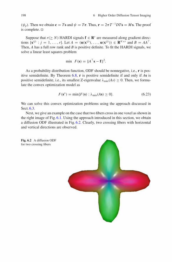
198 6 Higher Order Diffusion Tensor Imaging
(ψp). Then we obtain c = T s and ψ = Tr. Thus, r = 2πT −1DT s = M s. The proofis complete. ��
Suppose that r(≥ N ) HARDI signals f ∈ Rr are measured along gradient direc-tions {x(j) : j = 1, . . . , r}. Let A = (u(x(j)), . . . , u(x(j))) ∈ RN×r and B = AA�.Then, A has a full row rank and B is positive definite. To fit the HARDI signals, wesolve a linear least squares problem
min F(s) = ‖A�s − f‖2.
As a probability distribution function, ODF should be nonnegative, i.e., r is pos-itive semidefinite. By Theorem 6.8, r is positive semidefinite if and only if As ispositive semidefinite, i.e., its smallest Z-eigenvalue λmin(As) ≥ 0. Then, we formu-late the convex optimization model as
F(s∗) = min{F(s) : λmin(As) ≥ 0}. (6.23)
We can solve this convex optimization problems using the approach discussed inSect. 6.3.
Next, we give an example on the case that two fibers cross in one voxel as shown inthe right image of Fig. 6.1. Using the approach introduced in this section, we obtaina diffusion ODF illustrated in Fig. 6.2. Clearly, two crossing fibers with horizontaland vertical directions are observed.
Fig. 6.2 A diffusion ODFfor two crossing fibers
6.5 Nonnegative Fiber Orientation Distribution Function 199
6.5 Nonnegative Fiber Orientation Distribution Function
The spherical deconvolution (SD) model is another approach to capture crossingfibers in a voxel of biological tissues. Compared with Q-ball imaging, SD meth-ods impose a different assumption: all the nerve fibers share a common responsefunction. Hence, the ODF generated by SD is usually called the fiber orientationdistribution function or FOD. Using HARDI signals, the spherical deconvolutionmodel [265] expresses the signal attenuation as a convolution of the FOD and thecommon response function
S(x)/S0 =∫
S
f (v)R(x, v) dv, (6.24)
where v is an orientation of a nerve fiber, f (v) is the FOD to be estimated, andR(x, (0, 0, 1)�) is the common response function corresponding to HARDI signalsof a typical fiber with the orientation (0, 0, 1)�. To the sense of statistics, the FODshould be nonnegative
f (v) ≥ 0, ∀ v ∈ S (6.25)
and has a unit-mass ∫
S
f (v) dv = 1. (6.26)
Let the FOD function be a homogeneous polynomial f (v) = A vm, where Ais a symmetric tensor and m is even for symmetry. To deal with the nonnegativeconstraint (6.25), our basic idea is to restrict A as a sum-of-squares (SOS) tensor.We collect independent elements of the SOS tensor A in a vector w ∈ RN , andrewrite the FOD as
f (v) = u(x)�w.
Suppose that u(v) is a basis of m/2th order homogeneous polynomials in v. Then,there exists a positive semidefinite matrix X such that
f (v) = u(v)�X u(v).
Furthermore, there is a linear map A such that w = A(X ). In this way, we relax (6.25)as
w = A(X ) and X � 0. (6.27)
We consider the unit-mass constraint (6.26). It can be rewritten as
∫
S
f (v) dv =∫
S
N∑
j=1
wjuj(v) dv =N∑
j=1
wj
∫
S
uj(v) dv︸ ︷︷ ︸
:=sj
= 1.

200 6 Higher Order Diffusion Tensor Imaging
Hence, we rewrite the unit-mass constraint as
w�s = 1. (6.28)
The involved integrals in the vector s = (sj) could be calculated exactly using theMATLAB symbolic integration.
Suppose that HARDI measures r gradient directions x(i) and generates corre-sponding signals S(i) for i = 1, . . . , r. We represent the SD equation (6.24) similarly
S(i)/S0 =∫
S
N∑
j=1
wjφj(v) R(x, v) dv =N∑
j=1
wj
∫
S
φj(v)R(x, v) dv︸ ︷︷ ︸
γij
.
Denote f = (S(i)/S0) ∈ Rr . Due to the full rank assumption, the deconvolutionmatrix Γ = (γij) has a full column rank. Then, the SD fitting could be rewritten as
f ≈ Γ w. (6.29)
For the response function corresponding to a single fiber, we employ the bipolarWatson function [286]
R(x, v) = limα→+∞ exp[−α(x�v)2].
It is a refined Gaussian response corresponding to MRI signal attenuation of a signalfiber, as long as α is large enough.
Taking all the components (6.27)–(6.29) together, we obtain a convex semidefiniteprogramming model ⎧
⎪⎨
⎪⎩
min 12‖f − Γ w‖2
s.t. w = A(X ), X � 0,
w�s = 1.
(6.30)
This convex semidefinite programming model could be solved efficient by alternatingdirection methods of multipliers [49].
We now consider the case of two fibers crossing as shown in the right image inFig. 6.1. Using the model (6.30), we obtain a fiber ODF illustrated in Fig. 6.3. Clearly,there are two crossing fibers with horizontal and vertical directions.
Finally, we study a real-world human brain HARDI data. Each voxel is of size1.875 × 1.875 × 2 mm3, the diffusion-weighted b-value is b = 3000 s/mm2, and200 gradient directions are equipped.
For instance, we select a coronal slice of a healthy human brain, whose fractionalanisotropy (FA) map is reported in Fig. 6.4. The interesting region is marked by ayellow box. We illustrate detailed contour profiles of estimated FOD for this area inFig. 6.5. From this figure, we find that there are three nervous fibers detected in this
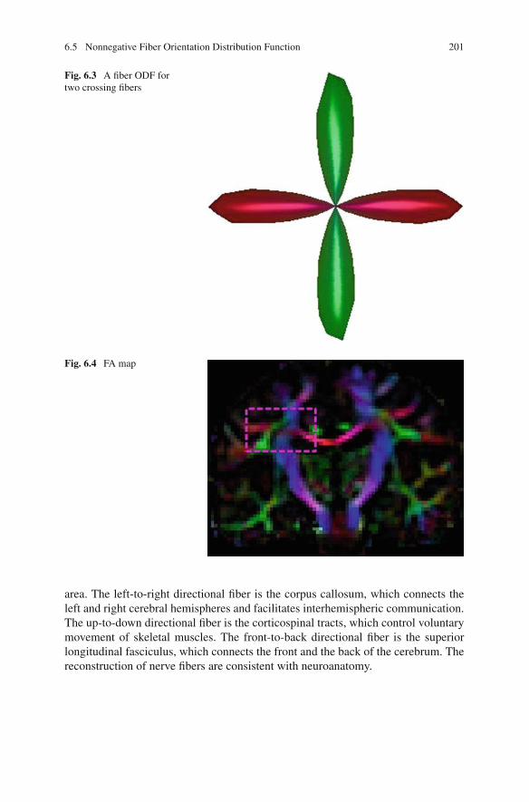
6.5 Nonnegative Fiber Orientation Distribution Function 201
Fig. 6.3 A fiber ODF fortwo crossing fibers
Fig. 6.4 FA map
area. The left-to-right directional fiber is the corpus callosum, which connects theleft and right cerebral hemispheres and facilitates interhemispheric communication.The up-to-down directional fiber is the corticospinal tracts, which control voluntarymovement of skeletal muscles. The front-to-back directional fiber is the superiorlongitudinal fasciculus, which connects the front and the back of the cerebrum. Thereconstruction of nerve fibers are consistent with neuroanatomy.

202 6 Higher Order Diffusion Tensor Imaging
Fig. 6.5 The reconstruction of corpus callosum crossing corticospinal tracts for the interestingregion
6.6 Image Authenticity Verification
In imaging science [302, 304], the directional characteristic of illumination in animage could be measured by the skewness of oriented gradients. Therefore, weintroduce the gradient skewness tensor (GST) to describe the third order statisticsof gradients. The estimating local directional characteristic of illumination can bemodeled as solving the largest D-eigenvalue of the corresponding GST.
Now, we give the definition of GST, which involves a third order symmetric tensorand a second order symmetric tensor from image gradients. By applying two 1-Dfilters in both directions such as
(−1 0 1)
and
⎛
⎝−101
⎞
⎠ ,
we obtain the horizontal and vertical gradient matrices of an image I denoted by Gx
and Gy, respectively. The oriented gradient matrix Gθ for a fixed angle θ ∈ [0, 2π)
is defined asGθ = Gx · cos θ + Gy · sin θ.
For a rectangle region L in the image I , we denote Gθ,L = (g1, g2, . . . , gn) asall gradient values of Gθ within the region L written in vector form, and Gx,L =(x1, x2, . . . , xn) and Gy,L = (y1, y2, . . . , yn) similarly for horizontal and vertical

6.6 Image Authenticity Verification 203
gradients Gx and Gy respectively. Let g be the mean of Gθ,L, the skewness of Gθ,L
is defined as
s(θ) =1nΣn
i=1(gi − g)3
(1nΣn
i=1(gi − g)2)3/2 , (6.31)
and it is a function of θ . Because of
gi = xi cos θ + yi sin θ
for a fixed θ , we haveg = x cos θ + y sin θ,
where x and y is the mean of Gx,L, and Gy,L. Therefore, the skewness function isrepresented as
s(θ) =1n
∑ni=1((xi cos θ + yi sin θ) − (x cos θ + y sin θ))3
(1n
∑ni=1((xi cos θ + yi sin θ) − (x cos θ + y sin θ))2
)3/2
=1n
∑ni=1((xi − x) cos θ + (yi − y) sin θ)3
( 1n
∑ni=1((xi − x) cos θ + (yi − y) sin θ)2)3/2
.
(6.32)
Furthermore, we define a series of discrete moments
μp,q =∑n
i=1(xi − x)(yi − y)
n
for p, q = 0, 1, 2, 3,. We can get another form of (6.32),
s(θ) = μ3,0 cos3 θ + 3μ2,1 cos2 θ sin θ + 3μ1,2 cos θ sin2 θ + μ0,3 sin3 θ
(μ2,0 cos2 θ + 2μ1,1 cos θ sin θ + μ0,2 sin2 θ)3/2. (6.33)
Consequently, we get the skewness function s(θ) which represents the skewnessvalue of image gradients for angle θ in the region L.
We use x = (cos θ, sin θ)� to denote the direction vector. By (6.33), we get
s(x) = μ3,0x31 + 3μ2,1x2
1x2 + 3μ1,2x1x22 + μ0,3x3
2
(μ2,0x21 + 2μ1,1x1x2 + μ0,2x2
2)3/2
. (6.34)
Then, the gradient skewness tensor A is a third order two dimensional symmetrictensor with elements
a111 = μ3,0,
a112 = a121 = a211 = μ2,1,
a122 = a212 = a221 = μ1,2,
a222 = μ0,3.
(6.35)

204 6 Higher Order Diffusion Tensor Imaging
A related second order symmetric tensor is
D =(
μ2,0 μ1,1
μ1,1 μ0,2
).
From (6.31), D is positive definite when all gradients within the region are not thesame everywhere, and this situation is easily satisfied in natural images. As a result,the skewness function s(x) can be written as
s(x) = A x3
(Dx2)3/2.
By optimization theory, the problem
max s(x) = A x3
(Dx2)3/2
is just equivalent to solving the largest D-eigenvalue of M , i.e., the solution of thesystem of equations: {
A x2 = λDx,
Dx2 = 1.
6.7 Notes
Starting from the basic model of DTI [9, 10], there are mainly two directions involv-ing tensors in our opinion. The first one is to develop rotation invariant indices ofnon-Gaussian diffusion of water molecules, such as D-eigenvalues of diffusion kur-tosis tensor, mean kurtosis, fractional kurtosis anisotropy [229], Z-eigenvalues ofgeneralized diffusion tensor, PSDT mean value, PSDT fractional anisotropy [231],and so on. The second one is trying to obtain the inherent fiber orientations of nervefibers in biological tissues. Typical examples are the diffusion ODF estimated byQ-ball imaging [232] and the fiber ODF estimated by spherical deconvolution model[49], where the involved higher order tensors are positive semidefinite. To extract fiberorientations, tensor-based methods were established [2, 18]. Additionally, Schultzet al. [239] wrote a review paper on higher order tensors in MRI.
Section 6.1 In DKI, Qi, Wang and Wu [229] considered the problem of max-imizing the apparent kurtosis coefficient Kapp and proposed the definition of D-eigenvalues. They proved that D-eigenvalues are invariant under orthogonal trans-formations. Hence, D-eigenvalues of the diffusion kurtosis tensor, as well as the meankurtosis and the fractional kurtosis anisotropy, are valuable indexes for medical imag-ing. Cui, Dai and Nie [66] gave an efficient numerical method for all D-eigenvaluesof a symmetric real tensor.

6.7 Notes 205
Han, Qi, and Wu [116] studied the largest diffusion value and the associated diffu-sion direction of water molecules in biological tissues by the following optimizationmodel ⎧
⎨
⎩max Dx2 − 1
6bMD2W x4
s.t. x�x = 1, x ∈ R3.
They pointed out that the extreme diffusion values are also invariant under orthogonaltransformations.
For real-world diffusion tensors and diffusion kurtosis tensors derived from MRIexperiments on rat spinal cord specimen fixed in formalin, plenty of results onD-eigenvalues of the diffusion kurtosis tensors and associated D-eigenvectors arereported in [227, 229, 288, 308].
Section 6.2 Owing to the signal attenuation in the MRI process, the estimateddiffusion tensor and kurtosis tensor should satisfy
bDx2 − 16 b2MD2W x4 > 0
for all directions x and b-values b ∈ (0, b]. This is a semi-infinite programmingproblem. Hu, Huang, Ni and Qi [128] established an exact conic linear optimizationmodel for the positive definiteness of diffusion kurtosis imaging.
Section 6.3 The diffusion kurtosis imaging used a second order diffusion tensorand a fourth order kurtosis tensor. Can we combine these two tensors into one tensor?That is the generalized diffusion tensor [215], whose order is even and may great thanfour. Qi, Yu and Wu [231] studied the positive definite generalized diffusion tensorimaging. Chen, Dai, Han and Sun [50] approximated the positive definite generalizeddiffusion tensor by a sum-of-squares tensor. If the order of the generalized diffusiontensor is four, this approximation is exact.
Section 6.4 To estimate the inherent fiber orientations of nerve fibers in biologicaltissues, Tuch [266] proposed the Q-ball imaging to estimate diffusion orientationdistribution function. Qi, Yu and Xu [232] applied nonnegative tensors for enforcingnonnegative diffusion orientation distribution function.
Section 6.5 The spherical deconvolution [265] is another method to estimate theinherent fiber orientations of nerve fibers in biological tissues. Chen, Dai and Han[49] employed a sum-of-squares polynomial to approximate the fiber orientationdistribution function.
Section 6.6 Another important application of D-eigenvalues is for image authen-ticity verification. Zhang, Zhou and Peng [302] explored skewness of oriented gra-dients to detect local illumination. By using the D-eigenvector corresponding to thelargest D-eigenvalue of the skewness tensor of oriented gradients, Zhang, Zhou andPeng [303, 304] proposed a novel approach for local illumination detection.
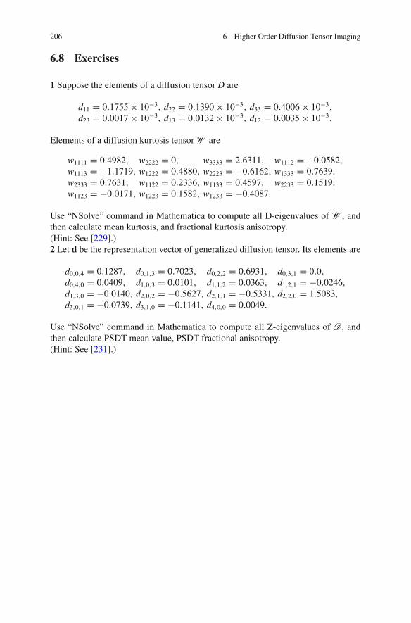
206 6 Higher Order Diffusion Tensor Imaging
6.8 Exercises
1 Suppose the elements of a diffusion tensor D are
d11 = 0.1755 × 10⁻³, d22 = 0.1390 × 10⁻³, d33 = 0.4006 × 10⁻³,
d23 = 0.0017 × 10⁻³, d13 = 0.0132 × 10⁻³, d12 = 0.0035 × 10⁻³.
Elements of a diffusion kurtosis tensor W are
w1111 = 0.4982, w2222 = 0, w3333 = 2.6311, w1112 = −0.0582,
w1113 = −1.1719, w1222 = 0.4880, w2223 = −0.6162, w1333 = 0.7639,
w2333 = 0.7631, w1122 = 0.2336, w1133 = 0.4597, w2233 = 0.1519,
w1123 = −0.0171, w1223 = 0.1582, w1233 = −0.4087.
Use “NSolve” command in Mathematica to compute all D-eigenvalues of W , andthen calculate mean kurtosis, and fractional kurtosis anisotropy.(Hint: See [229].)2 Let d be the representation vector of generalized diffusion tensor. Its elements are
d0,0,4 = 0.1287, d0,1,3 = 0.7023, d0,2,2 = 0.6931, d0,3,1 = 0.0,
d0,4,0 = 0.0409, d1,0,3 = 0.0101, d1,1,2 = 0.0363, d1,2,1 = −0.0246,
d1,3,0 = −0.0140, d2,0,2 = −0.5627, d2,1,1 = −0.5331, d2,2,0 = 1.5083,
d3,0,1 = −0.0739, d3,1,0 = −0.1141, d4,0,0 = 0.0049.
Use “NSolve” command in Mathematica to compute all Z-eigenvalues of D , andthen calculate PSDT mean value, PSDT fractional anisotropy.(Hint: See [231].)
Chapter 7Third Order Tensors in Physics andMechanics
Third order tensors have wide applications in physics and mechanics. Examplesinclude piezoelectric tensors in crystal study, third order symmetric traceless tensorsin liquid crystal study and third order susceptibility tensors in nonlinear optics study.On the other hand, the Levi-Civita tensor is famous in tensor calculus.
In 2017, Qi [225] studied third order tensors and hypermatrices systematically, byregarding a third order tensor as a linear operator which transforms a second ordertensor into a first order tensor, or a first order tensor into a second order tensor. Fora third order tensor, its transpose, kernel tensor, L-inverse and nonsingularity aredefined in [225]. Especially, the transpose of a third order tensor is uniquely defined.Note that the transpose of the piezoelectric tensor is the inverse piezoelectric tensor(the electrostriction tensor). Furthermore, the kernel tensor of a third order tensor isa second order positive semi-definite symmetric tensor, which is the product of thatthird order tensor and its transpose. A third order tensor has an L-inverse if and onlyif it is nonsingular. Here, “L” is named after Levi-Civita. Qi [225] also defined L-eigenvalues, singular values, C-eigenvalues and Z-eigenvalues for a third order tensor.They are all invariants of the third order tensor. A third order tensor is nonsingularif and only if all of its L-eigenvalues are positive. Physical meanings of these newconcepts were discussed. Qi showed that the Levi-Civita tensor is nonsingular, itsL-inverse is a half of itself, and its three L-eigenvalues are all the square root oftwo. Qi [225] also introduced third order orthogonal tensors. Third order orthogonaltensors are nonsingular as well, and their L-inverses are their transposes.
Piezoelectricity was discovered by Jacques Curie and Pierre Curie in 1880 [70].In the next year, the converse piezoelectric effect was predicted by Lippmann [182]and confirmed by Curies [71] immediately. Now they have wide applications in theproduction and detection of sounds, generation of high voltages, electronic frequencygeneration, microbalances, driving an ultrasonic nuzzle, and ultrafine focusing ofoptical assemblies.
In the piezoelectric effect and the converse piezoelectric effect, the piezoelectrictensor, a third order three dimensional partially symmetric tensor, plays a key role. A
© Springer Nature Singapore Pte Ltd. 2018L. Qi et al., Tensor Eigenvalues and Their Applications, Advances in Mechanicsand Mathematics 39, https://doi.org/10.1007/978-981-10-8058-6_7
207

208 7 Third Order Tensors in Physics and Mechanics
third order real tensor is called a piezoelectric-type tensor if it is partially symmetricwith respect to its last two indices. The piezoelectric tensor is a piezoelectric-typetensor of dimension three.
In 2017, Chen, Jákli and Qi [51] addressed C-eigenvalues and C-eigenvectorsfor piezoelectric-type tensors. Here, “C” names after Curie brothers (See Fig. 7.2).They showed that C-eigenvalues, which are invariant under orthonormal transfor-mations, always exist. For a piezoelectric-type tensor, the largest C-eigenvalue andits C-eigenvectors form the best rank-one piezoelectric-type approximation of thattensor. This means that for the piezoelectric tensor, its largest C-eigenvalue deter-mines the highest piezoelectric coupling constant. They further showed that for thepiezoelectric tensor, the largest C-eigenvalue corresponds to the electric displace-ment vector with the largest 2-norm in the piezoelectric effect under unit uniaxialstress and the strain tensor with the largest 2-norm in the converse piezoelectriceffect under unit electric field vector. Thus, C-eigenvalues and C-eigenvectors haveconcrete physical meanings in the piezoelectric effect and the converse piezoelectriceffect. Chen, Jákli and Qi [51] also studied computational methods for C-eigenvaluesand C-eigenvectors of the piezoelectric tensor for various crystal classes.
Liquid crystals are well-known for visualization applications of flat panel elec-tronic displays. Beyond that, various optical and electronic devices, such as laserprinters, light-emitting diodes, field-effect transistors, and holographic data storage,were invented with the development of bent-core (banana-shaped) liquid crystals. Tocharacterize condensed phases exhibited by these bent-core molecules, a third orderthree dimensional symmetric traceless tensor was employed. Based on such a tensor,the orientationally ordered octupolar (tetrahedratic) phase has been predicted theo-retically and confirmed experimentally. Whereafter, the octupolar order parametersof liquid crystals are widely studied.
In 2015 and 2016, Virga [270] and Gaeta and Virga [99] studied third orderoctupolar tensors in two and three dimensions, respectively. The octupolar potential,a scalar-valued function of the octupolar tensor, was also introduced. In particular,Gaeta and Virga [99] declared that the admissible region of the octupolar potential iswithin the form of a dome and there are two generic octupolar states, divided by theseparatrix surface, in the space of these three parameters. Such a separatrix surfacemay physically represent an intra-octupolar transition.
In 2017, utilizing the resultant theory in algebraic geometry and the E-characteristicpolynomial in spectral theory of tensors [228], Chen, Qi and Virga [52] gave the alge-braic expressions of the dome and the separatrix surface explicitly. This may turnsuch an intra-octupolar transition an observable prediction.
7.1 Third Order Tensors and Hypermatrices
In this section, we regard a tensor as a linear operator with dimension 3. Vectorsin R3 are denoted as xi , yi , zi , . . . , and matrices are denoted as ui j , vi j , . . . , whereindices i and j range from 1 to 3. For a product of vectors and matrices, if one index

7.1 Third Order Tensors and Hypermatrices 209
Table 7.1 Operators for second order tensors
No. Tensor operators Matrix operators
1 xU = y xi ui j = y j
2 x = Uy xi = ui j y j
3 U = x ⊗ y ui j = xi y j
4 xUy xi ui j y j
5 U • V ui j vi j
6 W = UV wi j = uikvk j
is repeated twice, we calculate the sum on this index. This is the common usage inthe literature of physics and mechanics. If we single out one vector or one matrix,their indices can be substituted with any other ones. However, if we address a productor a relation, or an equation of vectors and matrices, indices therein are related, andcannot be changed arbitrarily. In this hypermatrix notation, the Kronecker symbolδi j denotes the identity matrix. A square matrix pi j is called orthogonal if it satisfiespik p jk = δi j .
In a three dimensional physical space H, small bold letters x, y, z, . . . denotefirst order tensors. First order tensors have linear operators, i.e., additions amongthemselves and multiplications with scalars. Hence, there must be a first order zerotensor 0. For any x, y ∈ H, there exists a scalar x • y that satisfies the inner productrules, and H is complete with regard to this inner product. Then, H is a Hilbert spacemathematically. Thus, x • y is called the inner product of x and y. If x • y = 0,x and y are orthogonal. If x • x = 1, x is a first order unit tensor. Let {e1, e2, e3}be an orthonormal basis. Under this basis, two first order tensors x and y in H arerepresented by two vectors xi and yi in R3, respectively. Then we get
x • y = xi yi .
The summation value xi yi is independent from the choice of the orthonormal basis.The first order tensor x, which satisfies x•x = 0 is called a zero tensor 0. It is alwaysrepresented by the zero vector, and vice versa.
Second order tensors on H are denoted as capital bold letters U, V, . . . . We denoteB(H) the set of all second order tensors on H. Under an orthonormal basis {e1, e2, e3},a second order tensor U is represented by a matrix ui j in R3×3. Assume that a firstorder tensor x is represented by xi under this basis. Suppose that we have anotherorthonormal basis {g1, g2, g3}. Under {g1, g2, g3}, x and U are represented by a vectorzq in R3 and a matrix vqr in R3×3, respectively. Then there is an orthogonal matrix piq ,which is determined by these two bases, such that xi = piq zq and ui j = piq p jr vqr .
Second order tensors are physical quantities. They also have linear operators.There exists a second order zero tensor O . Suppose that U, V, W ∈ B(H), x, y ∈ H
are represented by ui j , vi j , wi j , xi and y j under an orthonormal basis, respectively.These operations can be described in Table 7.1.

210 7 Third Order Tensors in Physics and Mechanics
We note that the tensor U = x ⊗ y is called a second order rank-one tensor. Thevalue of U • V is also independent from the choice of the basis, and called the innerproduct of U and V. The second order tensor W = UV is called the product of Uand V.
For U ∈ B(H), if there is y ∈ H, y �= 0 such that Uy = 0, U is called a secondorder singular tensor. Otherwise, U is called nonsingular.
For any U ∈ B(H), there exists a unique second order tensor U� ∈ B(H) suchthat for any x, y ∈ H, xUy = yU�x. This second order tensor U� is coined thetranspose of U. Clearly, under an orthonormal basis, if U is represented by ui j , itstranspose U� must be represented by u ji . Moreover, for any U ∈ B(H), we have(U�)� = U. A second order tensor U is nonsingular if and only if U� is nonsingular.If U = U�, then U is called a symmetric tensor. If U = −U�, then U is calledan anti-symmetric tensor. Under an orthonormal basis, symmetric tensors and anti-symmetric tensors are always represented by symmetric matrices and anti-symmetricmatrices respectively.
If U = UV for any U ∈ B(H), then V is called the second order identity tensor,and denoted by I. For any U ∈ B(H), we also have U = IU. The identity tensor I isrepresented by δi j .
If UV = I, we say V is the inverse tensor of U, and denote it as U−1. A secondorder tensor U has an inverse tensor if and only if it is nonsingular. The inverse tensoris unique if it exists, and we always have (U−1)−1 = U.
If UU� = I, U is named an orthogonal tensor. Hence, an orthogonal tensor U isnonsingular, and U−1 = U�. A second order tensor is orthogonal if and only if itsrepresentative matrix is orthogonal.
Because the value of U • V is independent from the choice of the basis, for anyU ∈ B(H), U • I is independent from the choice of the basis, and is called the traceof U. The representation of U • I is uii under an orthonormal basis. A second ordertensor is called a traceless tensor if its trace is zero.
We say that U and V are orthogonal if U • V = 0. If U • U = 1, then U is calleda second order unit tensor.
If there exist a scalar λ and a first order nonzero tensor y such that Uy = λy, λ iscalled an eigenvalue of U and y is called the associated eigenvector. The eigenvalue λ
of U is independent from the choice of the basis. A sufficient and necessary conditionfor a second order tensor being nonsingular is that this tensor has no zero eigenvalue.There are three real eigenvalues of a second order symmetric tensor. The eigenvectorsassociated with different eigenvalues of a second order symmetric tensor are mutuallyorthogonal.
For a given U ∈ B(H), {y ∈ H : Uy = 0} forms a linear subspace of H, which iscalled the null space of U. We define the rank of U as 3 minus the dimension of thenull space of U.
Eigenvalues of a second order tensor are invariants of the tensor. For a secondorder symmetric tensor U, its trace is the sum of its eigenvalues, and the determinantof any of its representative matrix is equal to the product of its eigenvalues. Hence,this determinant is also an invariant of that tensor, and can be called the determinant
7.1 Third Order Tensors and Hypermatrices 211
of the tensor. This is also true for second order nonsymmetric tensors. The discussionof this may involve complex eigenvalues.
Let U be a second order symmetric tensor. We say that U is positive semi-definiteif for any first order tensor x ∈ H, xUx ≥ 0. Moreover, we say that U is positivedefinite if for any nonzero x ∈ H, we have xUx > 0. The tensor U is positive semi-definite if and only if all of its eigenvalues are nonnegative. The tensor U is positivedefinite if and only if all of its eigenvalues are positive.
Now, we turn to third order tensors. We use ai jk, bi jk, . . . with triple indices todenote 3 × 3 × 3 hypermatrices, where the indices i, j and k range from 1 to 3. Ahypermatrix ai jk is called orthogonal if
ai jkal jk = δil .
Third order tensors on H are denoted as calligraphic letters A ,B, . . . , and T (H)
stands for the set of third order tensors on H. When we discuss products of two thirdorder tensors, we may also refer to a fourth order tensor that is also denoted by acalligraphic letter T .
Under an orthonormal basis {e1, e2, e3}, a first order tensor x in H is representedby a three dimensional vector xi , a second order tensor U on H is represented by a3-by-3 matrix ui j , a third order tensor A is represented by a 3-by-3-by-3 hypermatrixai jk . Let {g1, g2, g3} be another orthonormal basis. Under that basis, assume that x,U, and A are represented by yq , vqr , and bqrs in R3, respectively. In fact, there existsan orthogonal matrix piq , which is only dependent on these two bases, such thatxi = piq yq , ui j = piq p jr vqr , and ai jk = piq p jr pksbqrs .
A third order tensor is also a physical quantity. They also have linear operations.Thus, there is a third order zero tensor O . Let A ,B ∈ T (H), U, V ∈ B(H), x, y, z ∈H, and a fourth order tensor T be represented by ai jk, bi jk, ui j , v jk, xi , y j , zk and ti jkl
under an orthonormal basis, respectively. Some of these operations can be describedin Table 7.2.
The third order tensor x ⊗ y ⊗ z is called a rank-one tensor. The value of A • Bis called the inner product of A and B. The tensor A B is called the second ordertensor product of A and B, and A ⊕ B is called the fourth order tensor product ofA and B.
Under an orthonormal basis {e1, e2, e3} of H, A ∈ T (H) is represented by ahypermatrix ai jk . That is to say,
ai jk = eiA e j ek .
Note that {−e1,−e2,−e3} is also an orthonormal basis of H. Under the sameorthonormal basis, A could also be represented by hypermatrix
−eiA (−e j )(−ek) = −ai jk .
212 7 Third Order Tensors in Physics and Mechanics
Table 7.2 Operations for third order tensors
No. Tensor operators Matrix operators
1 xA = V xi ai jk = v jk
2 U = A z ui j = ai jk zk
3 UA = z ui j ai jk = zk
4 x = A V xi = ai jkv jk
5 xyA = z xi y j ai jk = zk
6 xA z = y xi ai jk zk = y j
7 x = A yz xi = ai jk y j zk
8 A = U ⊗ z ai jk = ui j zk
9 A = x ⊗ V ai jk = xi v jk
10 A = x ⊗ y ⊗ z ai jk = xi y j zk
11 xA yz xi ai jk y j zk
12 A • B ai jkbi jk
13 U = A B uil = ai jkb jkl
14 T = A ⊕ B ti jkl = ai jmbmkl
A third order tensor A ∈ T (H) is named a singular tensor if there exists a firstorder nonzero tensor x ∈ H such that xA = O . Otherwise, A is called a nonsingulartensor.
For any y, z ∈ H, if A yz = A zy, then the third order tensor A ∈ T (H)
is called right-side symmetric. Under an orthonormal basis, if the tensor A isrepresented by ai jk , then we have ai jk = aik j for all i, j , and k. A typical example ofa third order right-side symmetric tensor is the piezoelectric tensor in solid crystals;See Sect. 7.3. However, in liquid crystals, the piezoelectric tensor is not right-sidesymmetric generically.
A third order tensor A ∈ T (H) is called left-side symmetric if for any x, y ∈ H,we have xyA = yxA . Under an orthonormal basis, if A is represented by ai jk , wehave ai jk = a jik . Inverse piezoelectric tensor is a typical example of a third orderleft-side symmetric tensor.
A third order tensor A ∈ T (H) is called left-side anti-symmetric if for anyx, y ∈ H, xyA = −yxA . Under an orthonormal basis, if A is represented by ai jk ,then we have ai jk = −a jik for all i, j and k. A typical example of a third orderleft-side anti-symmetric tensor is the Hall tensor.
A third order tensor A ∈ T (H) is called right-side anti-symmetric if for anyy, z ∈ H, A yz = −A zy. A third order tensor A ∈ T (H) is called centrally anti-symmetric if for any x, z ∈ H, xA z = −zA x. If a third order tensor A ∈ T (H)
is right-side, left-side and centrally anti-symmetric, the tensor is called totally anti-symmetric.
The Levi-Civita tensor E , which can be called the permutation tensor, is afamous example of third order three dimensional totally anti-symmetric tensors.Under a certain orthonormal basis, E is represented by the Levi-Civita hypermatrix
7.1 Third Order Tensors and Hypermatrices 213
εi jk , whose elements are ε123 = ε312 = ε231 = 1, ε213 = ε321 = ε132 = −1and εi jk = 0 otherwise. Other third order three dimensional totally anti-symmetrictensors are multiples of the Levi-Civita tensor. Then, the representative hypermatrixof the the Levi-Civita tensor E is either εi jk or −εi jk .
For any x, y, z ∈ H, we assume that A ,B ∈ T (H) satisfy xA yz = yBzx. Thenwe call B the transpose tensor of A and denote B = A �.
Proposition 7.1 Let A ∈ T (H). Then its transpose exists and is unique. Further-more, we always have [(A �)�]� = A .
We say that A is cyclically symmetric, if A � = A . Then the Levi-Civita tensoris a cyclically symmetric tensor. If for any x, y, z ∈ H, xA yz is invariant underany permutation of the positions of x, y and z, then we say that A is a third ordersymmetric tensor. A hypermatrix ai jk is called symmetric if ai jk is invariant underany change of its indices. Clearly, a third order tensor is symmetric if and only if itsrepresented hypermatrix is symmetric under an orthonormal basis. It is also easy toknow that a third order tensor is symmetric if and only if it is both right-side andcyclically symmetric.
If A A � = I, then we call A a third order three dimensional orthogonal tensor.Since the representative matrix of I is δi j , we have a proposition.
Proposition 7.2 Let A ∈ T (H). Then A is an orthogonal tensor if and only if itsrepresentative hypermatrix is orthogonal, under an orthonormal basis.
Let A ∈ T (H) and U = A A �. Then U is called the kernel tensor of A .
Theorem 7.1 Let U ∈ B(H) be a kernel tensor of A ∈ T (H). Then U is symmet-ric and positive semi-definite. Moreover, U is positive definite if and only if A isnonsingular. Specially, a third order orthogonal tensor is nonsingular.
The kernel tensor U = A A � is uniquely determined by A . Thus, some invariantsof U, such as the trace and the determinant of U, are also invariants of A . We callthe rank of U as the rank of A .
Let A and B be two third order three dimensional tensors on H. We say that Bis an L-inverse of A , if A and B satisfy
A B = I (7.1)
andB ⊕ A = A � ⊕ (B�)�. (7.2)
Moreover, we denote that B = A −1.
Theorem 7.2 (1) For a third order tensor A , we assume that its L-inverse exists.Then such an L-inverse is unique, denoted as A −1. Moreover, we have (A −1)−1 =A .
(2) The tensor A has an L-inverse if and only if A is nonsingular.(3) If A A � = tI for some t > 0, then A is nonsingular, and A −1 = 1
t A�. In
particular, A −1 = A � if A is an orthogonal tensor.

214 7 Third Order Tensors in Physics and Mechanics
Fig. 7.1 Tullio Levi-Civita(1873–1941)
Here, the letter “L” is named after Levi-Civita (see Fig. 7.1). We argue that theconcept of L-inverse is different from the Moore–Penrose inverse of a rectangularmatrix. The Moore–Penrose inverse of a rectangular always exists. However, the L-inverse of a third order tensor exists if and only if the tensor is nonsingular. Second,the L-inverse is a tensor concept. It is corresponding to the transformation from a firstorder tensor to a second order tensor. The Moore–Penrose inverse of a rectangularmatrix does not have such a property. An application of L-inverse confirms this.
Proposition 7.3 Suppose that A −1 of a third order tensor A exists and the followingtensor relation holds:
A z = U.
Then we obtainz = A −1U.
A typical example satisfying A z = U is the inverse piezoelectric effect, whereA is the inverse piezoelectric tensor, z is the electric field strength and U is thedeformation. Thus, if A −1 exists, we may calculate z from U.
Let A ∈ T (H), V ∈ B(H), x ∈ H and σ ∈ R. If σ ≥ 0 satisfies
A V = σx, A �x = σV, V • V = 1, x • x = 1, (7.3)

7.1 Third Order Tensors and Hypermatrices 215
σ is an L-eigenvalue of A , V and x are associated L-eigentensor and L-eigenvectorrespectively.
Theorem 7.3 Let A ∈ T (H). Then A has three L-eigenvalues σ1 ≥ σ2 ≥ σ3 ≥ 0,with associated L-eigentensors V1, V2, V3, and L-eigenvectors x1, x2, x3, respec-tively. The following assertions hold.
(1) Vi • V j = δi j and xi • x j = δi j .(2) Let U = A A � be the kernel tensor of A , which has eigenvalues λ1 ≥ λ2 ≥ λ3.
Then σ 2j = λ j for j = 1, 2, 3, and x j for j = 1, 2, 3 are associated eigenvectors
of U. Hence, L-eigenvalues of A are invariants of the tensor A .(3) We obtain
A =3∑
j=1
σ j x j ⊗ V j . (7.4)
(4) A −1 exists if and only if σ1 ≥ σ2 ≥ σ3 > 0. In this case, we know
A −1 =3∑
j=1
1
σ jV j ⊗ x j . (7.5)
(5) We getσ1 = max{√(A V) • (A V) : V • V = 1}. (7.6)
(6) If A is right-side symmetric, its L-eigentensors associated with a positive L-eigenvalue are symmetric.
(7) If A A � = αI for some α ≥ 0, then the L-eigenvalues of A are σ1 = σ2 = σ3 =√α. In particular, if A is a third order orthogonal tensor, then its L-eigenvalues
are all ones, i.e., σ1 = σ2 = σ3 = 1.
If A A � = αI for some α ≥ 0, then the three L-eigenvalues of A are the same.On the other hand, if the three L-eigenvalues of a third order tensor A are the same,do we always have A A � = αI for some α ≥ 0?
We call formulas (7.4) and (7.5) the L-eigenvalue decomposition of A and itsL-inverse. We do not say that 1
σ jfor j = 1, 2, 3 are L-eigenvalues of A −1, as A −1
may have different L-eigenvalues.We do not call σ j ( j = 1, 2, 3) singular values, although they are associated
with the singular value decomposition theory of rectangular matrices. One reason isthat they are third order tensors, but not rectangular matrices. They are only associ-ated with rectangular matrices unfolded from the representative hypermatrices withrespect to the last two indices. If we unfold the related hypermatrices with respectto the other two indices, results may be different. The second reason is that singularvalues for third order tensors will be defined later.
Given a third order tensor A ∈ T (H), a linear subspace {V ∈ B(H) : A V = 0}is called the null space of A . We have the following proposition.

216 7 Third Order Tensors in Physics and Mechanics
Proposition 7.4 Let A ∈ T (H). The dimension of the null space of A is at least 6.The sum of the rank and the dimension of this null space is 9.
This proposition means that the null space of a third order tensor is quite “large”,because its dimension is at least 6.
Suppose that A ∈ T (H), x, y, z ∈ H and η ∈ R. We say that η is a singularvalue of the tensor A , x, y and z are associated left, central and right singular vectorsrespectively if η ≥ 0 and the following system of equations hold.
A yz = ηx, xA z = ηy, xyA = ηz, x • x = 1, y • y = 1, z • z = 1. (7.7)
Theorem 7.4 Let A ∈ T (H). Then singular values of A always exist and areinvariants of A . Let η be a singular value of A , with associated left, central, andright singular vectors x, y, and z. Then η = xA yz. For the maximum singular valueη1 of A , we have
η1 = max{xA yz : x • x = 1, y • y = 1, z • z = 1}. (7.8)
Assume that A ∈ T (H), x, y,∈ H and μ ∈ R. We say that μ is a C-eigenvalueof A , x and y are associated left and right C-eigenvectors respectively if μ ≥ 0 andthe following system of equations hold.
A yy = μx, xA y = μy, x • x = 1, y • y = 1. (7.9)
C-eigenvalues were introduced in [51] for third order right-side symmetric tensors.We may extend them to general third order tensors; See Sect. 7.2. Here, “C” namesafter Jacques Curie and Pierre Curie (see Fig. 7.2).
Theorem 7.5 Let A ∈ T (H) be right-side symmetric. Then A always has C-eigenvalues that are invariants of A . Let μ be a C-eigenvalue of A with associatedleft and right C-eigenvectors x and y. Then μ = xA yy. Let μ1 be the maximumC-eigenvalue of A . Then we get
μ1 = max{xA yy : x • x = 1, y • y = 1}. (7.10)
By comparing (7.10) with (7.8), we have μ1 ≤ η1 for a third order right-side sym-metric tensor A .
Next, we recall the definition of Z-eigenvalues of a tensor A . Suppose that A ∈T (H), x,∈ H and ν ∈ R. We say that ν is a Z-eigenvalue of A with an associatedZ-eigenvector x, if ν ≥ 0 and the following system of equations hold.
A xx = νx, x • x = 1. (7.11)
Theorem 7.6 Let A ∈ T (H) be symmetric. Then Z-eigenvalues of A alwaysexist and are invariants of A . Let ν be a Z-eigenvalue of A with an associated
7.1 Third Order Tensors and Hypermatrices 217
Fig. 7.2 Pierre Curie(1859–1906)
Z-eigenvector x. Then ν = xA xx. Let ν1 be the maximum Z-eigenvalue of A . Then
ν1 = max{xA xx : x • x = 1}. (7.12)
Comparing (7.12) with (7.8) and (7.10), we have ν1 ≤ μ1 ≤ η1 for a third ordersymmetric tensor A . If A is symmetric, then ν1 = μ1.
We address more about the Levi-Civita tensor E .
Theorem 7.7 The Levi-Civita tensor E is a nonsingular tensor. The kernel tensorof E is 2I, the L-inverse is E −1 = 1
2E , and its three L-eigenvalues are σ1 = σ2 =σ3 = √
2. For any z ∈ H, if U = E z, then z = 12E U. Furthermore, 1√
2E is a third
order orthogonal tensor.
Now, the question is what the largest singular value of E is?We have known that right-side symmetry and left-side symmetry are tensor prop-
erties. Some tensor symmetric properties by using the Levi-Civita tensor could bedefined. Let ai jk be a hypermatrix. The hypermatrix ai jk is selectively right-side

218 7 Third Order Tensors in Physics and Mechanics
symmetric if ai jk = aik j for i �= k and i �= j . Similarly, the hypermatrix ai jk isselectively left-side symmetric if ai jk = a jik for k �= i and i �= k �= j .
Proposition 7.5 Suppose A ∈ T (H). Under an orthonormal basis, the represen-tative hypermatrix of A is selectively right-side symmetric if and only if A E = O ,and the representative hypermatrix of A is selectively left-side symmetric if andonly if E A = O . Thus, both the selectively right-side symmetric property and theselectively left-side symmetric property are tensor properties.
7.2 C-Eigenvalues of the Piezoelectric Tensors
We consider a special kind of tensors, named piezoelectric-type tensors, which is thegeneralization of right-side symmetric tensor.
Definition 7.1 Suppose that A = (ai jk) ∈ T3,n . If A is symmetric with respect toits last two indices, i.e., ai jk = aik j for all i , j , and k, then A is called a piezoelectric-type tensor. In particular, if n = 3, A is a right-side symmetric tensor.
The total number of independent elements of a piezoelectric-type tensor A is12 n2(n + 1).
Suppose that λ is a real number and x, y ∈ Rn are unit vectors. We say apiezoelectric-type tensor A is a rank-one tensor if its elements are ai jk = λxi y j yk
for i, j, k = 1, 2, . . . , n. Shortly, we denote this rank-one piezoelectric-type tensoras λx ⊗ y ⊗ y ∈ Tm,n , where “⊗” stands for the outer product. If there exist a scalarλ ∈ R and vectors x, y ∈ Rn minimizing the optimization problem
min{‖A − λx ⊗ y ⊗ y‖2
F : λ ∈ R, x�x = 1, y�y = 1}, (7.13)
then the tensor λx⊗y⊗y is called the best rank-one piezoelectric-type approximationof A .
By these notations, we represent the definition of C-eigenvalues and C-eigenvectorsof a piezoelectric tensor formally.
Definition 7.2 Suppose that A ∈ T3,n is a piezoelectric-type tensor. If there exist ascalar λ ∈ R and vectors x ∈ Rn and y ∈ Rn satisfying
A yy = λx, xA y = λy, x�x = 1, and y�y = 1, (7.14)
then λ is called a C-eigenvalue of A , x and y are called its associated left and rightC-eigenvectors, respectively. (λ, x, y) is called a C-eigentriple of A .
Immediately, we get the following theorem.
Theorem 7.8 Suppose that A is a piezoelectric-type tensor. The following threeassertions hold.

7.2 C-Eigenvalues of the Piezoelectric Tensors 219
(1) The piezoelectric-type tensor A has at least one C-eigentriple.(2) Suppose that (λ, x, y) is a C-eigentriple of A . Then
λ = xA yy.
Moreover, (λ, x,−y), (−λ,−x, y), and (−λ,−x,−y) are also C-eigentriplesof A .
(3) Let (λ∗, x∗, y∗) be a C-eigentriple of A , where λ∗ is the largest C-eigenvalue ofA . Then
λ∗ = max {xA yy : x�x = 1, y�y = 1}. (7.15)
Furthermore, the tensor λ∗x∗ ⊗ y∗ ⊗ y∗ is the best rank-one piezoelectric-typeapproximation of A .
Theorem 7.8 (c) implies that the largest C-eigenvalue λ∗ determines the high-est piezoelectric coupling constant, and y∗ is the direction of the stress where thisappears. In the sense of this point, the largest C-eigenvalue of a piezoelectric tensorhas concrete physical meaning.
The invariant property under orthogonal transformations is important for manyphysical problems. Next, we are going to show that C-eigenvalues of a piezoelectric-type tensor A = (ai jk) are invariant under orthogonal transformations. Let A be apiezoelectric-type tensor and Q = (qir ) ∈ Rn×n be an orthogonal matrix. Then, therotated tensor A Q3 is also a piezoelectric-type tensor.
Theorem 7.9 Suppose that Q ∈ Rn×n is an orthogonal matrix and A ∈ T3,n is apiezoelectric-type tensor. Let (λ, x, y) be a C-eigentriple of A . Then, (λ, Q�x, Q�y)
is a C-eigentriple of A Q3.
Next, we address two intervals for locating all C-eigenvalues of piezoelectric-typetensors, which provide upper bounds for the largest C-eigenvalue [166].
Theorem 7.10 Let A ∈ T3,n be a piezoelectric-type tensor, and λ be one of itsC-eigenvalues. Then, we have
|λ| ≤ κ1(A ), (7.16)
wherer (1)
i (A ) :=∑
j,k∈[n]|ai jk |, r (2)
j (A ) :=∑
i,k∈[n]|ai jk |,
and
κ1(A ) := maxi, j∈[n]
√r (1)
i (A )r (2)j (A ).
Proof Since λ is a C-eigenvalue of A , we assume that x = (xi ) ∈ Rn and y =(yi ) ∈ Rn are associated left and right C-eigenvectors. Denote that
|x p| = maxi∈[n] |xi | ∈ (0, 1] and |yq | = max
i∈[n] |yi | ∈ (0, 1].

220 7 Third Order Tensors in Physics and Mechanics
Considering the pth equation of A yy = λx, we obtain
λx p =∑
j,k∈[n]apjk y j yk,
and hence
|λ||x p| ≤∑
j,k∈[n]|apjk ||y j |yk |,
≤∑
j,k∈[n]|apjk ||yq ||yq |
≤ |yq |r (1)p (A ). (7.17)
In a similar way, we have|λ||yq | ≤ |x p|r (2)
q (A ). (7.18)
Multiplying (7.17) and (7.18) and eliminating a factor |x p||yq | > 0, we get
|λ|2 ≤ r (1)p (A )r (2)
q (A ) ≤ maxi, j∈[n] r (1)
i (A )r (2)j (A ).
Let κ1(A ) = maxi, j∈[n]√
r (1)i (A )r (2)
j (A ). Then the proof is complete. �
From this theorem, κ1(A ) is an upper bound for the largest C-eigenvalue of apiezoelectric-type tensor.
Let S be a subset of [n]. Denote that
ΩS := {(i, j) : i ∈ S or j ∈ S},Ωc
S := {(i, j) : i /∈ S and j /∈ S}.
For a given piezoelectric-type tensor A ∈ T3,n , we define
rΩSk (A ) :=
∑
(i, j)∈ΩS
|ai jk |,
rΩc
Sk (A ) :=
∑
(i, j)∈ΩcS
|ai jk |.
Here, rΩSk (A ) = 0 if S = ∅, and r
ΩcS
k (A ) = 0 if S = [n]. Moreover, we have
r (2)k (A ) = rΩS
k (A ) + rΩc
Sk (A ). Define
rS(A ) := maxi, j∈[n]
1
2
(rΩS
j (A ) +√
(rΩSj (A ))2 + 4r (1)
i (A )rΩc
Sj (A )
),

7.2 C-Eigenvalues of the Piezoelectric Tensors 221
for any subset S of [n], and
κ2(A ) := minS⊆[n] rS(A ).
Then, we have another bound for λ.
Theorem 7.11 Suppose that λ is a C-eigenvalue of a piezoelectric-type tensor A ∈T3,n. Then, we get
|λ| ≤ κ2(A ).
Proof Let S be a subset of [n]. We assume that x = (xi ) ∈ Rn and y = (yi ) ∈ Rn areleft and right C-eigenvectors of A corresponding to the C-eigenvalue λ. We denote
|x p| = maxi∈[n] |xi | ∈ (0, 1] and |yq | = max
i∈[n] |yi | ∈ (0, 1].
Considering the qth equation of xA y = λy, we have
|λ||yq | =∣∣∣∣∣∣
∑
i, j∈[n]ai jq xi y j
∣∣∣∣∣∣
≤∑
i, j∈[n]|ai jq ||xi ||y j |
≤ |x p||yq |∑
i, j∈[n]|ai jq |
≤ |x p||yq |(rΩSq (A ) + r
ΩcS
q (A ))
≤ rΩSq (A )|yq | + r
ΩcS
q (A )|x p|.
Thus,(|λ| − rΩS
q (A ))|yq | ≤ rΩc
Sq (A )|x p|. (7.19)
By multiplying (7.17) and (7.19) and eliminating |x p||yq |, it yields that
|λ|(|λ| − rΩSq (A )) ≤ r (1)
p (A )rΩc
Sq (A ).
Then, we solve the above inequality and get
|λ| ≤ 1
2
(rΩS
q (A ) +√
(rΩSq (A ))2 + 4r (1)
p (A )rΩc
Sq (A )
)≤ rS(A ).
Because |λ| ≤ rS(A ) is valid for all S ⊆ [n], we obtain this theorem. �
Note that κ2(A ) is also an upper bound of the largest C-eigenvalue of apiezoelectric-type tensor A . By setting S = ∅, we find that
222 7 Third Order Tensors in Physics and Mechanics
κ2(A ) ≤ r∅ = maxi, j∈[n]
√r (1)
i (A )r (2)j (A ) = κ1(A ).
Hence, the upper bound of the largest C-eigenvalue of a piezoelectric-type tensorobtain by Theorem 7.11 is sharper than the upper bound established in Theorem7.10.
In physics, for non-centrosymmetric materials, the linear piezoelectric equationis expressed as
pi =3∑
j,k=1
ai jk Tjk,
where A = (ai jk) is a third order piezoelectric tensor, T = (Tjk) ∈ R3×3 isthe second order stress tensor, and p = (pi ) ∈ R3 is the electric change densitydisplacement (polarization), which is a first order tensor. Since A is a piezoelectric-type tensor, there are 18 independent elements in A .
Under a unit uniaxial stress, what situations will trigger the maximal piezoelec-tricity? An idea example of uniaxial stress is the stress in a long, vertical rod loadedby hanging a weight on the end [212, p. 90]. In this case, the second order stress ten-sor could be rewritten as T = yy� with y�y = 1. Then, we formulate this maximalpiezoelectricity problem into an optimization model
⎧⎪⎨
⎪⎩
max ‖p‖2
s.t. p = A yy,
y�y = 1.
(7.20)
By a dual norm, we know ‖p‖2 = maxx�x=1 x�p = maxx�x=1 xA yy. Hence, itsuffices to consider the following optimization problem
max xA yy s.t. x�x = 1, y�y = 1. (7.21)
Assume that (x∗, y∗) is an optimal solution of the above optimization problem. Then,the optimal value of objective λ∗ = x∗A y∗y∗ is the largest C-eigenvalue of the piezo-electric tensor A , and y∗ is the unit uniaxial direction that the maximal piezoelectriceffect take place along. These results imply the following theorem.
Theorem 7.12 Suppose that (λ∗, x∗, y∗) is a C-eigentriple of the piezoelectric tensorA , and λ∗ is the largest C-eigenvalue of A . Then, under a unit uniaxial stress, themaximum value of the 2-norm of the electric polarization is λ∗ and the optimal axialdirection is y∗.
We turn to the converse piezoelectric effect and consider the following linearequation
Sjk =∑
i
ai jkei ,

7.2 C-Eigenvalues of the Piezoelectric Tensors 223
where S = (Sjk) ∈ R3×3 is the strain tensor and e = (ei ) ∈ R3 is the electric fieldstrength. Denote ‖ · ‖2 as the matrix spectral norm, i.e., ‖S‖2 = maxy�y=1 y�Sy.
Now, we study the maximization problem on the spectral norm of S:
⎧⎪⎪⎪⎪⎨
⎪⎪⎪⎪⎩
max ‖S‖2
s.t. Sjk =3∑
i=1
ei ai jk ∀ j, k ∈ {1, 2, 3},
e�e = 1.
(7.22)
Since ‖S‖2 = maxy�y=1 y�Sy = maxy�y=1 eA yy, we could rewrite (7.22) asfollows:
max {eA yy : e�e = 1, y�y = 1}.
Let (e∗, y∗) be an optimal solution of the above optimization problem. Then, λ∗ =e∗A y∗y∗ is the largest C-eigenvalue of the piezoelectric tensor A , e∗ and y∗ are itsassociated left and right C-eigenvectors.
Theorem 7.13 Suppose that (λ∗, x∗, y∗) is a C-eigentriple of the piezoelectric ten-sor A and λ∗ is the largest C-eigenvalue. Then, under unit electric field strength‖x∗‖ = 1, λ∗ is the largest spectral norm of a strain tensor generated by the conversepiezoelectric effect.
Due to the crystallographic symmetry of piezoelectric materials, there are 32classes in crystals [119]. However, 11 classes of crystals enjoy the center of symmetry,hence there are no piezoelectricity. In addition, for a special class numbered 432,piezoelectric changes counteract each other. Thus, there remains 20 crystallographicclasses, where piezoelectricity may exist. We now examine some typical crystals inthese crystallographic classes.
By Theorem 7.8 (b), we know that (−λ,−x, y), (λ, x,−y), and (−λ,−x,−y) areall C-eigentriples of a piezoelectric tensor if (λ, x, y) is a C-eigentriple of this tensor.For compactness, we use (λ, x, y) to present the group of these four C-eigentriplesof the piezoelectric tensor.
Piezoelectric tensors of crystals have special symmetric structures microscopi-cally. First, we examine crystals in 23 and 43m crystallographic point groups. Thecorresponding piezoelectric tensor A (α) has only one independent parameter α > 0:
a123 = a213 = a312 = −α.
Other elements of A (α) are zeros.
Proposition 7.6 There are 13 groups of C-eigentriples of the piezoelectric tensorA (α).
Next, we present some C-eigentriples of piezoelectric tensors arising from knownpiezoelectric materials with different symmetries. All piezoelectric tensors measured
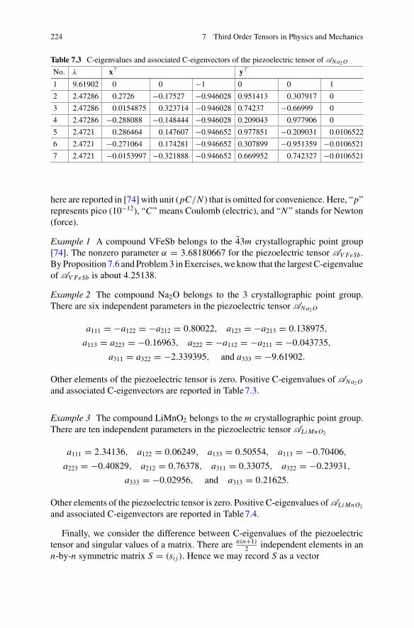
224 7 Third Order Tensors in Physics and Mechanics
Table 7.3 C-eigenvalues and associated C-eigenvectors of the piezoelectric tensor of ANa2 O
No. λ x� y�
1 9.61902 0 0 −1 0 0 1
2 2.47286 0.2726 −0.17527 −0.946028 0.951413 0.307917 0
3 2.47286 0.0154875 0.323714 −0.946028 0.74237 −0.66999 0
4 2.47286 −0.288088 −0.148444 −0.946028 0.209043 0.977906 0
5 2.4721 0.286464 0.147607 −0.946652 0.977851 −0.209031 0.0106522
6 2.4721 −0.271064 0.174281 −0.946652 0.307899 −0.951359 −0.0106521
7 2.4721 −0.0153997 −0.321888 −0.946652 0.669952 0.742327 −0.0106521
here are reported in [74] with unit (pC/N ) that is omitted for convenience. Here, “p”represents pico (10−12), “C” means Coulomb (electric), and “N” stands for Newton(force).
Example 1 A compound VFeSb belongs to the 43m crystallographic point group[74]. The nonzero parameter α = 3.68180667 for the piezoelectric tensor AV FeSb.By Proposition 7.6 and Problem 3 in Exercises, we know that the largest C-eigenvalueof AV FeSb is about 4.25138.
Example 2 The compound Na2O belongs to the 3 crystallographic point group.There are six independent parameters in the piezoelectric tensor ANa2 O
a111 = −a122 = −a212 = 0.80022, a123 = −a213 = 0.138975,
a113 = a223 = −0.16963, a222 = −a112 = −a211 = −0.043735,
a311 = a322 = −2.339395, and a333 = −9.61902.
Other elements of the piezoelectric tensor is zero. Positive C-eigenvalues of ANa2 O
and associated C-eigenvectors are reported in Table 7.3.
Example 3 The compound LiMnO2 belongs to the m crystallographic point group.There are ten independent parameters in the piezoelectric tensor ALi MnO2
a111 = 2.34136, a122 = 0.06249, a133 = 0.50554, a113 = −0.70406,
a223 = −0.40829, a212 = 0.76378, a311 = 0.33075, a322 = −0.23931,
a333 = −0.02956, and a313 = 0.21625.
Other elements of the piezoelectric tensor is zero. Positive C-eigenvalues of ALi MnO2
and associated C-eigenvectors are reported in Table 7.4.
Finally, we consider the difference between C-eigenvalues of the piezoelectrictensor and singular values of a matrix. There are n(n+1)
2 independent elements in ann-by-n symmetric matrix S = (si j ). Hence we may record S as a vector
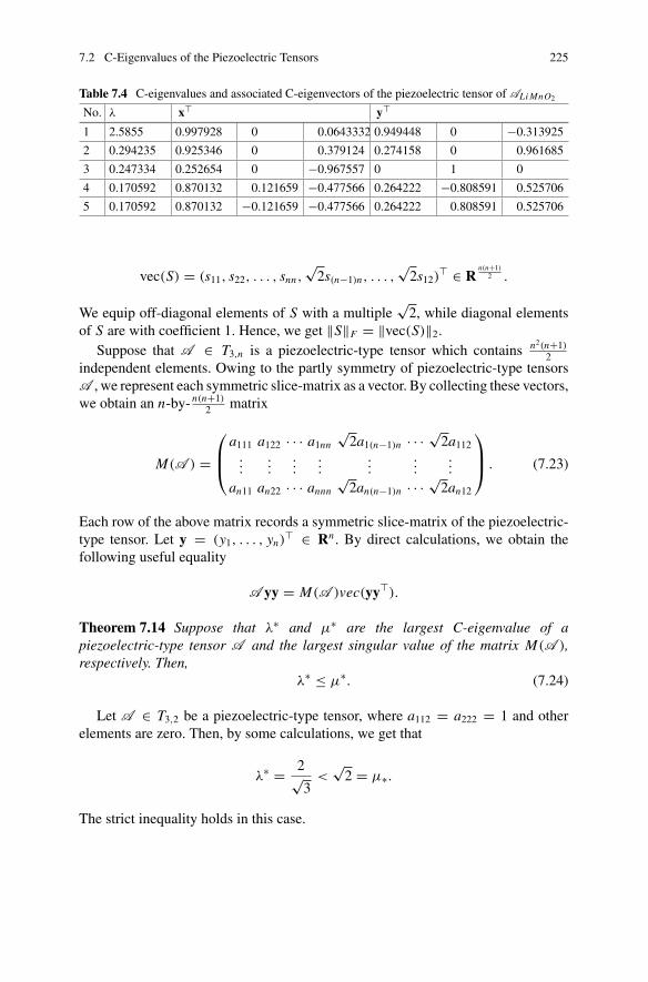
7.2 C-Eigenvalues of the Piezoelectric Tensors 225
Table 7.4 C-eigenvalues and associated C-eigenvectors of the piezoelectric tensor of ALi MnO2
No. λ x� y�
1 2.5855 0.997928 0 0.0643332 0.949448 0 −0.313925
2 0.294235 0.925346 0 0.379124 0.274158 0 0.961685
3 0.247334 0.252654 0 −0.967557 0 1 0
4 0.170592 0.870132 0.121659 −0.477566 0.264222 −0.808591 0.525706
5 0.170592 0.870132 −0.121659 −0.477566 0.264222 0.808591 0.525706
vec(S) = (s11, s22, . . . , snn,√
2s(n−1)n, . . . ,√
2s12)� ∈ R
n(n+1)
2 .
We equip off-diagonal elements of S with a multiple√
2, while diagonal elementsof S are with coefficient 1. Hence, we get ‖S‖F = ‖vec(S)‖2.
Suppose that A ∈ T3,n is a piezoelectric-type tensor which contains n2(n+1)
2independent elements. Owing to the partly symmetry of piezoelectric-type tensorsA , we represent each symmetric slice-matrix as a vector. By collecting these vectors,we obtain an n-by- n(n+1)
2 matrix
M(A ) =⎛
⎜⎝a111 a122 · · · a1nn
√2a1(n−1)n · · · √
2a112...
......
......
......
an11 an22 · · · annn
√2an(n−1)n · · · √
2an12
⎞
⎟⎠ . (7.23)
Each row of the above matrix records a symmetric slice-matrix of the piezoelectric-type tensor. Let y = (y1, . . . , yn)
� ∈ Rn . By direct calculations, we obtain thefollowing useful equality
A yy = M(A )vec(yy�).
Theorem 7.14 Suppose that λ∗ and μ∗ are the largest C-eigenvalue of apiezoelectric-type tensor A and the largest singular value of the matrix M(A ),respectively. Then,
λ∗ ≤ μ∗. (7.24)
Let A ∈ T3,2 be a piezoelectric-type tensor, where a112 = a222 = 1 and otherelements are zero. Then, by some calculations, we get that
λ∗ = 2√3
<√
2 = μ∗.
The strict inequality holds in this case.
226 7 Third Order Tensors in Physics and Mechanics
7.3 Third Order Three Dimensional Symmetric TracelessTensors and Liquid Crystals
In 1888, an Austrian botanist Friedrich Reinitzer (1857–1927) discovered liquid crys-tals which were further studied and named later by German physicist Otto Lehmann(1855–1922) in 1904. Liquid crystals are special matter in a state which has proper-ties between those of conventional liquids and solid crystals. A liquid crystal phaseof matter is described as one where constituent molecules are sufficiently disorderedto confer the flow properties of a liquid, yet still preserve some degree of orderingsuch that the phase is anisotropic. In recent advance of liquid crystals, the octupolar(tetrahedratic) phase for bent-core (banana-shaped) liquid crystals molecules is anovel phase that was predicted theoretically [24, 186] and confirmed experimentally[287].
Each liquid crystal molecule has a microscopic polar axis p. In a macroscopicmolecular assembly, we could consider the orientational distribution ρ of these polaraxes. By Buckingham’s formula [28], the probability density of an orientationaldistribution ρ : S2 �→ R+ over the unit sphere S2 = {p ∈ R3 : p�p = 1} could berepresented as
ρ(p) = 1
4π
(1 +
∞∑
k=1
(2k + 1)!!k! 〈p⊗k〉ρ · p⊗k
),
where p⊗k is a kth order rank-one tensor, 〈p⊗k〉ρ is the corresponding multipoleaverage, and the overline . . . denotes the irreducible, symmetric, and traceless partof the tensor it surmounted. As a probability density function, the spherical integral
∫
S2ρ(p)dp = 1,
which is equal to a spherical integral of the constant term 14π
. Hence, sphericalintegrals of other terms should be zero.
Particularly, the first three multipole averages are called the dipolar, quadrupolar,and octupolar order tensors
d = 〈p〉ρ, Q = 〈p ⊗ p〉ρ, A = 〈p ⊗ p ⊗ p〉ρ.
They are meaningful for resolving the characteristic features of ρ. Since their spher-ical integrals are zero, we know that Q is a symmetric and traceless matrix, andthe octupolar tensor A = (ai jk) is a third order three dimensional symmetric andtraceless tensor.
We now give the definition of traceless tensors formally.

7.3 Third Order Three Dimensional Symmetric Traceless Tensors and Liquid Crystals 227
Definition 7.3 Let T = (ti1i2...im ) ∈ Sm,n . If
n∑
i=1
tii i3...im = 0 for all i3, . . . , im = 1, 2, . . . , n,
then T is called a traceless tensor.
The following theorem shows that under orthogonal transformations, the tracelessproperty of a symmetric tensor is invariant [99].
Theorem 7.15 Let T = (ti1i2...im ) ∈ Sm,n be a traceless tensor and Q = (qi j ) ∈Rn×n be an orthogonal matrix. Then, T Qm is also a traceless tensor.
Proof It is straightforward to see that the new tensor T Qm is real-valued and sym-metric. Now, we consider its slice matrices. As the sum of all matrix eigenvalues, thetrace of a symmetric matrix is invariant under an orthogonal transformation. Hence,we get
n∑
i=1
m∑
j1=1
m∑
j2=1
t j1 j2 j3··· jm qi j1 qi j2 =n∑
i=1
tii j3··· jm = 0 (7.25)
for all j3, . . . , jm = 1, 2, . . . , n. By some calculations,
n∑
i=1
[T Qm]i i i3···im =n∑
i=1
n∑
j1=1
n∑
j2=1
n∑
j3=1
· · ·n∑
jm=1
t j1 j2 j3··· jm qi j1 qi j2 qi3 j3 · · · qim jm
=n∑
j3=1
· · ·n∑
jm=1
⎛
⎝n∑
i=1
n∑
j1=1
n∑
j2=1
t j1 j2 j3··· jm qi j1 qi j2
⎞
⎠ qi3 j3 · · · qim jm
= 0,
where the last equality is valid because of (7.25). Hence, the new tensor T Qm isalso traceless. �
In the remainder of this chapter, we focus on the octupolar tensor A . The sym-metry means that ten independent parameters are needed for presenting a genericoctupolar tensor, i.e.,
A =⎛
⎝a111 a112 a113 a112 a122 a123 a113 a123 a133
a112 a122 a123 a122 a222 a223 a123 a223 a233
a113 a123 a133 a123 a223 a233 a133 a233 a333
⎞
⎠ ∈ S3,3. (7.26)
The word “traceless” means that⎧⎪⎨
⎪⎩
a111 + a122 + a133 = 0,
a112 + a222 + a233 = 0,
a113 + a223 + a333 = 0.
(7.27)

228 7 Third Order Tensors in Physics and Mechanics
Hence, seven independent parameters are sufficient for describing a generic octupolartensor A .
For convenience, we denote seven independent parameters of the octupolar tensorA as
α0 = a123,
α1 = a111, α2 = a222, α3 = a333,
β1 = a122, β2 = a233, β3 = a113.
By the traceless property (7.27), we could rewrite (7.26) as
A =⎛
⎝α1 −α2 − β2 β3 −α2 − β2 β1 α0 β3 α0 −α1 − β1
−α2 − β2 β1 α0 β1 α2 −α3 − β3 α0 −α3 − β3 β2
β3 α0 −α1 − β1 α0 −α3 − β3 β2 −α1 − β1 β2 α3
⎞
⎠ .
Then, the associated octupolar potential defined on the unit sphere S2 [99] is
Φ(x) ≡ A x3 =3∑
i=1
3∑
j=1
3∑
k=1
ai jk xi x j xk (7.28)
= α1x31 + α2x3
2 + α3x33 + 6α0x1x2x3 + 3β1x1x2
2 + 3β2x2x23 + 3β3x2
1 x3
− 3(α1 + β1)x1x23 − 3(α2 + β2)x2
1 x2 − 3(α3 + β3)x22 x3.
We say that the potential Φ(x) has at least one maximum point on the unit sphereS2. Without loss of generality, we rotate the Cartesian coordinate system such thatthe maximum point being the North pole (0, 0, 1)�, i.e.,
α3 = Φ(0, 0, 1) ≥ 0.
From the spectral theory of tensors [221], α3 is a Z-eigenvalue of A with anassociated Z-eigenvector (0, 0, 1)�. Hence, all Z-eigenvectors λ and associated Z-eigenvalues x of A must satisfy the following system of Z-eigenvalues:
⎧⎪⎪⎪⎪⎨
⎪⎪⎪⎪⎩
α1x21 + 2α0x2x3 + β1x2
2 + 2β3x1x3 − (α1 + β1)x23 − 2(α2 + β2)x1x2 = λx1,
α2x22 + 2α0x1x3 + 2β1x1x2 + β2x2
3 − (α2 + β2)x21 − 2(α3 + β3)x2x3 = λx2,
α3x23 + 2α0x1x2 + 2β2x2x3 + β3x2
1 − 2(α1 + β1)x1x3 − (α3 + β3)x22 = λx3,
x21 + x2
2 + x23 = 1.
Hence, by substituting λ = α3 and x = (0, 0, 1)� to the above system, we obtain
α1 + β1 = 0 and β2 = 0.
Moreover, because Φ(x) is a continuous function and Φ(−x1, 0, 0) = −Φ(x1, 0, 0),we can rotate the Cartesian coordinate system so that Φ(1, 0, 0) = 0 and we get

7.3 Third Order Three Dimensional Symmetric Traceless Tensors and Liquid Crystals 229
α1 = 0.
In this way, we determined three parameters in A that are α1 = β1 = β2 = 0.Then, the octupolar tensor in (7.26) is indeed
A =⎛
⎝0 −α2 β3 −α2 0 α0 β3 α0 0
−α2 0 α0 0 α2 −α3 − β3 α0 −α3 − β3 0β3 α0 0 α0 −α3 − β3 0 0 0 α3
⎞
⎠ ,
which features four independent parameters: α0, α2, α3, and β3. Correspondingly,the octupolar potential (7.28) reduces to
Φ(x;α0, α2, α3, β3) = α2x32 + α3x3
3 + 6α0x1x2x3
+ 3β3x21 x3 − 3α2x2
1 x2 − 3(α3 + β3)x22 x3 (7.29)
for all x ∈ S2. Without loss of generality, we can assume
α2 ≥ 0
because of the symmetry revealed by the following proposition.
Proposition 7.7 For the octupolar potential (7.29), we get
Φ(x1, x2, x3;α0, α2, α3, β3) = Φ(x1,−x2, x3;−α0,−α2, α3, β3).
We exploit the assumption that the North pole (0, 0, 1)� is a maximum point ofthe octupolar potential Φ(x) on the unit sphere S2 with a value α3.
Theorem 7.16 Suppose that the North pole (0, 0, 1)� is a local maximum point ofΦ(x) on S2. Then, the following inequality holds
3α23 − 4α3β3 − 4β2
3 − 4α20 ≥ 0. (7.30)
If the strict inequality holds in (7.30), (0, 0, 1)� is a strict local maximum point ofΦ(x) on S2.
Proof We consider the spherical optimization problem:
{max Φ(x) = A x3
s.t. x�x = 1.(7.31)
Its Lagrangian is
L(x, λ) = −1
3A x3 + λ
2(x�x − 1).
The Hessian of the Lagrangian is

230 7 Third Order Tensors in Physics and Mechanics
∇2xx L(x, λ) = λI − 2A x,
which is positive semidefinite on the tangent space x⊥ ≡ {y ∈ R3 : x�y = 0} if xis a (local) maximum point of Φ(x) on S2 [211]. Let P ≡ I − xx� ∈ R3×3 be theprojection matrix onto x⊥. Then, the matrix P�∇2
xx L(x, λ)P is positive semidefinite.By use of the first-order necessary condition,
A x2 = λx and x�x = 1,
we have that
P�∇2xx L(x, λ)P = (I − xx�)(λI − 2A x)(I − xx�)
= λ(I − xx�) − 2(I − xx�)(A x)(I − xx�)
= λ(I − xx�) − 2(A x − x(A x2)� − (A x2)x� + (A x3)xx�)
= λ(I − xx�) − 2(A x − λxx� − λxx� + λxx�)
= λ(I + xx�) − 2A x. (7.32)
Because the North pole (0, 0, 1)� is a local maximum point with associated mul-tiplier λ = α3, we arrive at
[P�∇2xx L(x, λ)P]λ=α3,x=(0,0,1)� =
⎡
⎣α3 − 2β3 −2α0 0
−2α0 3α3 + 2β3 00 0 0
⎤
⎦ .
As easily seen, this projected Hessian has eigenvalues
μ1 = 0, μ2,3 = 2α3 ±√
(α3 + 2β3)2 + 4α20,
which are all required to be non-negative [211]. Hence, we obtain the followinginequality
3α23 − 4α3β3 − 4β2
3 − 4α20 ≥ 0.
If the strict inequality holds, i.e., if 3α23 − 4α3β3 − 4β2
3 − 4α20 > 0, then the North
pole (0, 0, 1)� is a strict local maximum point of Φ(x) on S2 [211]. �
In the case α3 = 0, we know that α0 = β3 = 0 by Theorem 7.16. If α2 > 0 holds,Φ(0, 1, 0) = α2 > α3 = Φ(0, 0, 1). This contradicts that the North pole (0, 0, 1)�is the maximum point. Hence we also have α2 = 0. The octupolar tensor A is atrivial zero tensor.
In the remainder, we shall consider the case that α3 is positive. Without loss ofgenerality, by Proposition 7.7 and Theorem 7.16, we can restrict our discussion onthe following admissive region
α3 = 1, α2 ≥ 0, and α20 + (β3 + 1
2 )2 ≤ 1. (7.33)
7.3 Third Order Three Dimensional Symmetric Traceless Tensors and Liquid Crystals 231
Then, there are three parameters in the octupolar tensor
A (α0, β3, α2) =⎛
⎝0 −α2 β3 −α2 0 α0 β3 α0 0
−α2 0 α0 0 α2 −1 − β3 α0 −1 − β3 0β3 α0 0 α0 −1 − β3 0 0 0 1
⎞
⎠ (7.34)
and the associated octupolar potential
Φ(x) = α2x32 + x3
3 + 6α0x1x2x3 + 3β3x21 x3 − 3α2x2
1 x2 − 3(1 + β3)x22 x3 (7.35)
for all x ∈ S2. In the following sections, we will give algebraic expressions of thedome surface and the separatrix surface of the octupolar tensor (7.34).
7.4 Algebraic Expression of the Dome Surface
On the unit sphere S2, we have assumed that the global maximum point of theoctupolar potential Φ(x) is the North pole (0, 0, 1)�; See Sect. 7.3. That is to say,λ = 1 is the largest Z-eigenvalue of the octupolar tensor A , and (0, 0, 1)� is anassociated Z-eigenvector. In the admissible cylinder (7.33), there is a reduced regionsuch that the maximal Z-eigenvalue of A (α0, β3, α2) is 1. The boundary of thisreduced admissible region is called the dome [99]: its apex is at (α0, β3, α2) =(0,− 1
2 ,√
22 ), and it meets the plane α2 = 0 along the circle α2
0 + β23 + β3 = 0. Next,
we try to find the algebraic expression of this dome.We introduce our main tool: the resultant from algebraic geometry [64]. We con-
sider a system of homogeneous polynomials f (x) = 0, where f (x) = ( f1(x), . . . ,
fn(x))� : Rn �→ Rn and each component fi (x) has positive degree di fori = 1, . . . , n. By algebraic geometry, the resultant of f is an irreducible polyno-mial RES( f ) in coefficients of f (x), which vanishes if and only if that polynomialsystem f (x) = 0 has nonzero solutions; and if fi (x) = xdi
i , the value of that resultantshould be 1.
For example, we consider a system of linear equations Ax = 0. Each componentfunction is a first order homogeneous polynomial. Then, the resultant is the determi-nant det(A). By linear algebra, we know that Ax = 0 has a nonzero solution if andonly if det(A) vanishes; and if A = I , then det(A) = 1.
For a system with only two variables
{f1(x, y) =am xm + am−1xm−1 y + · · · + a0 ym = 0,
f2(x, y) =b0xn + b1xn−1 y + · · · + bn yn = 0,
the resultant is the following determinant

232 7 Third Order Tensors in Physics and Mechanics
RES( f1, f2) =
∣∣∣∣∣∣∣∣∣∣∣∣∣∣
am am−1 · · · a0
. . .. . .
. . .. . .
am am−1 · · · a0
b0 b1 · · · bn
. . .. . .
. . .. . .
b0 b1 · · · bn
∣∣∣∣∣∣∣∣∣∣∣∣∣∣
.
By direct observation, we find that RES( f1, f2) is the determinant of the followingsystem ⎧
⎪⎪⎪⎪⎪⎪⎪⎪⎪⎪⎪⎨
⎪⎪⎪⎪⎪⎪⎪⎪⎪⎪⎪⎩
xn−1 f1(x, y) = 0,
...
yn−1 f1(x, y) = 0,
xm−1 f2(x, y) = 0,
...
ym−1 f2(x, y) = 0.
If the system f1(x, y) = f2(x, y) = 0 has non-trivial solutions, it goes the same forthe system above. Hence, the determinant RES( f1, f2) vanishes.
Next, we turn to the general cases. For simplicity, we take the resultant RES(A x2)
for example, where
A x2 =⎛
⎝−2α2x1x2 + 2β3x1x3 + 2α0x2x3
−α2x21 + α2x2
2 + 2α0x1x3 − 2(1 + β3)x2x3
β3x21 − (1 + β3)x2
2 + x23 + 2α0x1x2
⎞
⎠ ≡⎛
⎜⎝f3(x1, x2, x3)
f1(x1, x2, x3)
f2(x1, x2, x3)
⎞
⎟⎠ .
By the spectral theory of tensors, RES(A x2) is called the hyperdeterminant of theoctupolar tensor A [228].
The following process is a standard approach introduced in Chap. 3, Sect. 4 of[64]. Since the degree of each component homogeneous polynomial fi in variablesx1, x2, x3 is di = 2, we may set the total degree
d =3∑
i=1
(di − 1) + 1 = 4
and divide monomials xυ = xυ11 xυ2
2 xυ33 of total degree |υ| ≡ υ1 + υ2 + υ3 = 4 into
three sets:
S1 = {xυ : |υ| = d, x21 divides xυ } = {x4
1 , x31 x2, x3
1 x3, x21 x2
2 , x21 x2x3, x2
1 x23 },
S2 = {xυ : |υ| = d, x21 doesn’t divide xυ but x2
2 does} = {x1x32 , x1x2
2 x3, x42 , x3
2 x3, x22 x2
3 },S3 = {xυ : |υ| = d, x2
1 , x22 don’t divide xυ but x2
3 does} = {x1x2x23 , x1x3
3 , x2x33 , x4
3 }.

7.4 Algebraic Expression of the Dome Surface 233
Clearly, there exist(d+2
2
) = 15 monomials xυ with total degree 4 and each belongsto one of sets S1, S2, and S3, which are mutually disjoint. Then, the system of 15equations are listed here
⎧⎪⎨
⎪⎩
xυ/x21 · f1 = 0 for all xυ ∈ S1,
xυ/x22 · f2 = 0 for all xυ ∈ S2,
xυ/x23 · f3 = 0 for all xυ ∈ S3.
Its coefficient matrix D in the unknowns xυ with total degree 4 is
D =
⎛
⎜⎜⎜⎜⎜⎜⎜⎜⎜⎜⎜⎜⎜⎜⎜⎜⎜⎜⎜⎜⎜⎜⎜⎜⎝
−α2 2α0 α2 −2(1 + β3)
−α2 2α0 α2 −2(1 + β3)
−α2 2α0 α2
−α2 2α0
−α2
−α2
β3 2α0 −1 − β3
β3 2α0 −1 − β3
β3 2α0
β3 2α0
β3
−2α2 2β3 2α0
−2α2 2β3
−2α2
−2(1 + β3)
α2 −2(1 + β3)
α2 −2(1 + β3) 2α0
α2 2α0 −2(1 + β3)
11
−1 − β3 1−1 − β3 1
−1 − β3 2α0 1
2α0
2α0 2β3
−2α2 2β3 2α0
⎞
⎟⎟⎟⎟⎟⎟⎟⎟⎟⎟⎟⎟⎟⎟⎟⎟⎟⎟⎟⎟⎟⎟⎟⎟⎠
.
It has an important property that

234 7 Third Order Tensors in Physics and Mechanics
det(D) = RES(A x2) · extraneous factor.
A monomial xυ of total degree d = 4 is called reduced if x2i divides xυ for exactly
one i . Let D′ be the determinant of the submatrix of D obtained by deleting all rowsand columns corresponding to reduced monomials, i.e., in our context,
D′ =⎛
⎝−α2
−α2 α2
β3 −1 − β3
⎞
⎠ .
According to Theorem 4.9 in Chap. 3 of [64], to within a sign, the resultant RES(A x2)reads as
RES(A x2) = det D
det D′ (7.36)
= 16α22(48α8
0β3 + 4α60(α2
2 + β3(32β23 + 24β3 − 9)) + 3α4
0(α22(52β2
3 + 28β3 − 1)
+ 4β23 (8β3
3 + 8β23 − 9β3 − 9)) + 6α2
0(α42(4β3 + 1) − α2
2β3(14β33 + 36β2
3 + 35β3
+ 10) − 2β33 (β3 + 1)2(8β3 + 9)) + (α2
2 − 4(β3 + 1)3)(α22 − β2
3 (2β3 + 3))2).
Theorem 7.17 The hyperdeterminant of the octupolar tensor A is presented in(7.36). The system A x2 = 0 has nonzero solutions if and only if the hyperdeterminantvanishes, i.e., RES(A x2) = 0.
Next, we compute the E-characteristic polynomial φA (λ) of the octupolartensor (7.34), using the approach of resultants. By introducing an auxiliary x0, theE-characteristic polynomial φA (λ) is indeed a resultant of the following system ofhomogeneous polynomial equations:
⎧⎪⎪⎨
⎪⎪⎩
x21 + x2
2 + x23 − x2
0 = 0,
−α2x21 + α2x2
2 + 2α0x1x3 − 2(1 + β3)x2x3 − λx0x2 = 0,
β3x21 − (1 + β3)x2
2 + x23 + 2α0x1x2 − λx0x3 = 0,
−2α2x1x2 + 2β3x1x3 + 2α0x2x3 − λx0x1 = 0.
(7.37)
Using Mathematica, we get the explicit expression of the E-characteristic polynomialφA (λ).
Theorem 7.18 The E-characteristic polynomial of the octupolar tensor A in (7.34)is
φA (λ) = (λ2 − 1)
6∑
i=0
c2iλ2i ,
where, in particular,

7.4 Algebraic Expression of the Dome Surface 235
c0 = 256α42(48α8
0β3 + 4α60(α
22 + β3(32β2
3 + 24β3 − 9)) + 3α40(α
22(52β2
3
+ 28β3 − 1) + 4β23 (8β3
3 + 8β23 − 9β3 − 9)) + 6α2
0(α42(4β3 + 1)
− α22β3(14β3
3 + 36β23 + 35β3 + 10) − 2β3
3 (β3 + 1)2(8β3 + 9))
+ (α22 − 4(β3 + 1)3)(α2
2 − β23 (2β3 + 3))2)2.
Cartwright and Sturmfels [29] pointed out that if the tensor A ∈ Tm,n hasfinitely many equivalence classes of eigenpairs over complex field, then their number,counted with multiplicity, is equal to
(m − 1)n − 1
m − 2.
For a tensor A ∈ Tm,n , if (λ, x) satisfies A xm−1 = λx, then all (tm−2λ, t x) withfree t is called a equivalence class of A . In the context of the octupolar tensor, (λ, x)
and (−λ,−x) belong to the same equivalence class. Hence, the E-characteristicpolynomial of the octupolar tensor A should be a polynomial in λ of degree 14,which coincides with Theorem 7.18. Moreover, we find that the E-characteristicpolynomial φA (λ) has no odd-degree terms. By comparing the expression of c0 and(7.36), we get
c0 = [RES(A x2)
]2.
Theorem 7.19 We assume that A x2 = 0 has only the trivial solution x = 0. Then,the system (7.37) has a non-trivial solution (x0, . . . , x3) over C if and only if theE-characteristic polynomial φA (λ) = 0.
Corollary 7.1 If RES(A x2) �= 0, all E-eigenvalues of the octupolar tensor A arenon-zero.
Now, we are ready to give an explicit formula for the dome. Recalling the E-characteristic polynomial φA (λ) in Theorem 7.18, we can obtain that λ = 1 is itsroot. Since the dome is the locus where the maximal Z-eigenvalue is λ = 1, λ = 1is at least a double root of φA (λ). By substituting λ = 1 into φA (λ)/(λ2 − 1) = 0,we obtain the following equation
c1(α0, β3, α2)3 · c2(α0, β3, α2) · c3(α0, β3, α2) = 0, (7.38)
wherec1(α0, β3, α2) = 3 − 4α2
0 − 4β23 − 4β3,
c2(α0, β3, α2) = 64α42 −16α2
2(1+2β3)(−12α20 +(1+2β3)
2)+(4α20 +(1+2β3)
2)3,
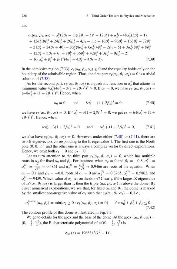
236 7 Third Order Tensors in Physics and Mechanics
and
c3(α0, β3, α2) = α62(2β3 − 1)((2β3 + 5)2 − 12α2
0) + α42(−48α4
0(3β23 − 1)
+ 12α20(8β4
3 + 24β33 + 26β2
3 − 4β3 − 11) − 16β63 − 96β5
3 − 168β43 − 72β3
3
− 21β23 − 24β3 + 40) + 8α2
2(8α60 + 6α4
0(4β23 − 2β3 − 5) + 3α2
0(8β43 + 8β3
3
− 12β23 − 3β3 + 6) + 8β6
3 + 36β53 + 42β4
3 + 3β33 − 9β2
3 − 2)
− 16(α20 + β2
3 + β3)2(4α2
0 + 4β23 + 4β3 − 3). (7.39)
In the admissive region (7.33), c1(α0, β3, α2) ≥ 0 and the equality holds only on theboundary of the admissible region. Thus, the first part c1(α0, β3, α2) = 0 is a trivialsolution of (7.38).
As for the second part, c2(α0, β3, α2) is a quadratic function in α22 that attains its
minimum value 4α20(4α2
0 − 3(1 + 2β3)2)2 ≥ 0. If α0 = 0, we have c2(α0, β3, α2) =
(−8α22 + (1 + 2β3)
3)2. Hence, when
α0 = 0 and 8α22 − (1 + 2β3)
3 = 0, (7.40)
we have c2(α0, β3, α2) = 0. If 4α20 − 3(1 + 2β3)
2 = 0, we get c2 = 64(α22 + (1 +
2β3)3)2. Hence, when
4α20 − 3(1 + 2β3)
2 = 0 and α22 + (1 + 2β3)
3 = 0, (7.41)
we also have c2(α0, β3, α2) = 0. However, under either (7.40) or (7.41), there aretwo E-eigenvectors corresponding to the E-eigenvalue 1. The first one is the Northpole (0, 0, 1)� and the other one is always a complex vector by direct explorations.Hence, we omit both c1 = 0 and c2 = 0.
Let us turn attention to the third part c3(α0, β3, α2) = 0, which has multipleroots in α2 for fixed α0 and β3. For instance, when α0 = 0 and β3 = −0.8, α
(1)2 =
α(2)2 = 2√
17≈ 0.4851 and α
(3)2 = 4
√7
5√
5≈ 0.9466 are roots of the equation. When
α0 = 0.1 and β3 = −0.8, roots of c3 = 0 are α(1)2 = 0.3765, α
(2)2 = 0.5862, and
α(3)2 = 9459. Which value of α2 lies on the dome? Clearly, if the largest Z-eigenvalue
of A (α0, β3, α2) is larger than 1, then the triple (α0, β3, α2) is above the dome. Bydirect numerical explorations, we see that, for fixed α0 and β3, the dome is markedby the smallest non-negative value of α2 such that c3(α0, β3, α2) = 0, i.e.,
α(dome)2 (α0, β3) = min{α2 ≥ 0 : c3(α0, β3, α2) = 0} for α2
0 + β23 + β3 ≤ 0.
(7.42)The contour profile of this dome is illustrated in Fig. 7.3.
We go to details for the apex and the base of the dome. At the apex (α0, β3, α2) =(0,− 1
2 ,√
22 ), the E-characteristic polynomial of A (0,− 1
2 ,√
22 ) is
φA (λ) = 19683λ6(λ2 − 1)4.

7.4 Algebraic Expression of the Dome Surface 237
Fig. 7.3 The dome that bounds the reduced admissible region as represented by (7.42)
Clearly, λ2 = 1 is a quadruple root of φA (λ), and hence it is a Z-eigenvalue of A .Four associated Z-eigenvectors are listed as follows:
x(1) = (0, 0, 1)�, x(2) =(
0, 2√
23 ,− 1
3
)�,
x(3) =(√
63 ,−
√2
3 ,− 13
)�, x(4) =
(−
√6
3 ,−√
23 ,− 1
3
)�.
The corresponding contour profile of the octupolar potential Φ(x) is illustrated inFig. 7.4a.
At the base of the dome, we know α2 = 0 and α20 +β2
3 +β3 = 0, which representsa circle of center in (α0, β3) = (0,− 1
2 ) and radius 12 . Then, the E-characteristic
polynomial reduces toφA (λ) = −64λ8(λ2 − 1)3.
Clearly, λ2 = 1 is a triple root of φA (λ). Specifically, the largest Z-eigenvalue λ = 1of A (0,−1, 0) has three Z-eigenvectors, namely,
x(1) = (0, 0, 1)�, x(2) =(−
√3
2 , 0,− 12
)�, x(3) =
(√3
2 , 0,− 12
)�.
In this case, the contour profile of the octupolar potential Φ(x) is shown in Fig. 7.4b.The two profiles in Fig. 7.4 illustrate the typical appearance of the octupolar potentialin two highly symmetric states.

238 7 Third Order Tensors in Physics and Mechanics
(a) A (0,− 12 ,
√22 ) (b) A (0,−1,0)
Fig. 7.4 Two typical (symmetric) polar plots of the octupolar potential
7.5 Algebraic Expression of the Separatrix Surface
Gaeta and Virga [99] pointed out that there exists a separatrix surface connecting twodifferent generic states of the octupolar potential Φ: Φ has four maxima and three(positive) saddles in one generic state; in the other generic state, Φ has three maximaand two (positive) saddles; See Fig. 7.4. Whereafter, we try to determine explicitlythe separatrix surface.
We recall the spherical optimization problem (7.31) in Sect. 7.3:
{max Φ(x) = A x3
s.t. x�x = 1.
Its projected Hessian (7.32) reads as
P�∇2xx L(x, λ)P = λ(I + xx�) − 2A x.
Clearly, this projected Hessian P�∇2xx L(x, λ)P has two zero eigenvalues. μ1 = 0 is
an eigenvalue of the projected Hessian with the associated eigenvector x. Supposethat μ2 and μ3 are the other two eigenvalues of the projected Hessian. Let σ ≡μ2μ3 = μ1μ2 + μ1μ3 + μ2μ3. Then, by linear algebra, σ is equal to the sum of all2-by-2 principal minors of the projected Hessian. By calculations, we get
σ = λ2(3 + 2x21 + 2x2
2 + 2x23 ) + 2λ
(α2x3
2 + x33 + 6α0x1x2x3 + 3β3x2
1 x3 − 3α2x21 x2
−3(1 + β3)x22 x3
)− 4
((α2
0 + α22 + β2
3 )x21 + (α2
0 + α22 + (β3 + 1)2)x2
2

7.5 Algebraic Expression of the Separatrix Surface 239
+(α20 + β2
3 + β3 + 1)x23 − 2α0x1x2 − 2α0α2x1x3 − α2(2β3 + 1)x2x3
)
= 7λ2 − 4((α2
0 + α22 + β2
3 )x21 + (α2
0 + α22 + (β3 + 1)2)x2
2 + (α20 + β2
3 + β3 + 1)x23
−2α0x1x2 − 2α0α2x1x3 − α2(2β3 + 1)x2x3) (7.43)= 0.
Furthermore, if λ �= 0 and x �= 0 satisfy A x2 = λx, λ‖x‖ and 1
‖x‖x satisfy the system
of Z-eigenvalues. Hence, we omit the spherical constraint x�x = 1 temporarily andjust focus on the system of homogeneous polynomial equations (7.43) and
⎧⎨
⎩
−2α2x1x2 + 2β3x1x3 + 2α0x2x3 − λx1 = 0,
−α2x21 + α2x2
2 + 2α0x1x3 − 2(1 + β3)x2x3 − λx2 = 0,
β3x21 − (1 + β3)x2
2 + x23 + 2α0x1x2 − λx3 = 0.
(7.44)
Using the resultant theory, we obtain the resultant of (7.43) and (7.44), which isthe separatrix:
1792(4α20 + 4β2
3 + 4β3 − 3)28∑
i=0
d2i (α0, β3)α2i2 = 0, (7.45)
where
d16 = 27(−16α40 − 8α2
0(4β23 − 44β3 + 13) − (2β3 − 1)(2β3 + 7)3),
d14 = −54(128α60 − 16α4
0(48β23 + 78β3 − 29) + 16α2
0(72β43 + 124β3
3 + 190β23
− 101β3 − 69) + (2β3 + 7)2(40β33 + 44β2
3 + 62β3 − 47)),
d12 = −9(4096α80 − 128α6
0(277β23 − 92β3 − 55) + 48α4
0(152β43 + 1944β3
3
− 7094β23 − 1548β3 + 53) + 8α2
0(5648β63 + 18912β5
3 + 60408β43 + 115368β3
3
+ 86625β23 − 44964β3 − 18410) − 1664β8
3 − 22400β73 − 124064β6
3
− 377088β53 − 624840β4
3 − 383256β33 + 109994β2
3 + 181940β3 − 17605),
d10 = −2(22528α100 + 256α8
0(800β23 + 3620β3 + 599) + 64α6
0(5440β43 − 195290β3
3
− 97221β23 − 44476β3 + 8375) + 16α4
0(12800β63 + 1073640β5
3 + 2832444β43
+ 2369838β33 − 242151β2
3 − 492540β3 − 270455) + 4α20(17920β8
3
− 1188320β73 − 6499376β6
3 − 13648368β53 − 10198728β4
3 + 1289514β33
+ 3579185β23 + 123260β3 + 206555) + 32768β10
3 + 483200β93 + 3111744β8
3
+ 10647136β73 + 19890064β6
3 + 19640424β53 + 5479324β4
3 − 6109790β33
− 3422445β23 + 504920β3 + 3560),
d8 = 5(40960α120 − 12288α10
0 (97β23 + 88β3 + 44) + 256α8
0(39921β43 + 34176β3
3
+ 42870β23 + 12132β3 + 1667) − 128α6
0(141080β63 + 419208β5
3 + 389430β43

240 7 Third Order Tensors in Physics and Mechanics
+ 82228β33 − 15613β2
3 − 100402β3 − 37063) + 48α40(212768β8
3 + 1023680β73
+ 1963504β63 + 1378192β5
3 − 304390β43 − 508976β3
3 + 63582β23 − 57076β3
− 52349) − 8α20(149376β10
3 + 1199488β93 + 4718496β8
3 + 9599232β73
+ 9822584β63 + 3227448β5
3 − 2548818β43 − 2029036β3
3 − 53961β23
+ 37902β3 − 40196) + (2β3 + 1)2(10304β103 + 154304β9
3 + 911472β83
+ 2786464β73 + 4828732β6
3 + 3895212β53 + 22345β4
3 − 1558688β33
− 352512β23 + 133184β3 − 7840)),
d6 = 16(28672α140 − 512α12
0 (688β23 + 1102β3 + 941) − 128α10
0 (9696β43
− 40380β33 − 33951β2
3 − 20148β3 − 11743) − 160α80(5632β6
3 − 26064β53
− 7644β43 + 35134β3
3 − 57181β23 − 51958β3 − 5454) + 40α6
0(18944β83
− 103552β73 − 737312β6
3 − 1217152β53 − 320576β4
3 + 504962β33 + 120149β2
3
− 112824β3 − 29175) + 2α40(577536β10
3 + 1111040β93 − 2474880β8
3
− 6705600β73 − 341600β6
3 + 9137976β53 + 5840100β4
3 − 884330β33
− 684765β23 + 374580β3 + 132449) + α2
0(2β3 + 1)2(80896β103 + 999808β9
3
+ 3452640β83 + 5398208β7
3 + 3717992β63 − 367068β5
3 − 2064016β43
− 746875β33 + 150774β2
3 + 30796β3 − 25928) − (2β3 + 1)4(2048β103
+ 25824β93 + 135752β8
3 + 385692β73 + 535154β6
3 + 253167β53
− 114083β43 − 118464β3
3 − 4364β23 + 7632β3 − 656)),
d4 = 16(−32768α160 + 2048α14
0 (241β23 − 284β3 − 83) + 256α12
0 (9208β43
− 5384β33 + 6390β2
3 + 25496β3 + 8589) + 128α100 (25680β6
3 − 32160β53
+ 7368β43 + 257000β3
3 + 212292β23 + 23286β3 − 10209) + 80α8
0(8064β83
− 169344β73 − 304224β6
3 + 311872β53 + 774736β4
3 + 306928β33 − 61620β2
3
− 34824β3 + 1209) − 8α60(281856β10
3 + 2529280β93 + 6835200β8
3
+ 6572800β73 + 316800β6
3 − 2303424β53 − 174400β4
3 + 593920β33
+ 124725β23 − 2310β3 + 6019) − 2α4
0(2β3 + 1)2(230144β103 + 1285120β9
3
+ 3244032β83 + 4304128β7
3 + 2583584β63 + 28128β5
3 − 669240β43
− 261024β33 + 369β2
3 + 30952β3 − 3232) − 4α20(2β3 + 1)4(5408β10
3
+ 10240β93 − 22272β8
3 − 72224β73 − 83578β6
3 − 75384β53 − 40635β4
3
+ 8889β33 + 10338β2
3 − 2444β3 − 184) + 2(β3 + 1)2(2β3 + 1)6(400β83 + 4000β7
3
+ 15408β63 + 16240β5
3 − 2449β43 − 6128β3
3 + 104β23 + 272β3 − 24)),
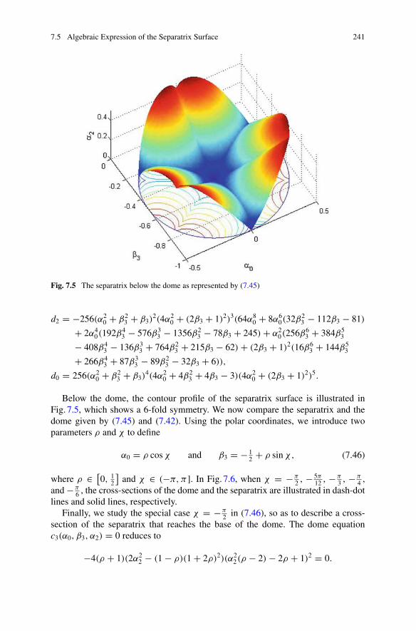
7.5 Algebraic Expression of the Separatrix Surface 241
Fig. 7.5 The separatrix below the dome as represented by (7.45)
d2 = −256(α20 + β2
3 + β3)2(4α2
0 + (2β3 + 1)2)3(64α80 + 8α6
0(32β23 − 112β3 − 81)
+ 2α40(192β4
3 − 576β33 − 1356β2
3 − 78β3 + 245) + α20(256β6
3 + 384β53
− 408β43 − 136β3
3 + 764β23 + 215β3 − 62) + (2β3 + 1)2(16β6
3 + 144β53
+ 266β43 + 87β3
3 − 89β23 − 32β3 + 6)),
d0 = 256(α20 + β2
3 + β3)4(4α2
0 + 4β23 + 4β3 − 3)(4α2
0 + (2β3 + 1)2)5.
Below the dome, the contour profile of the separatrix surface is illustrated inFig. 7.5, which shows a 6-fold symmetry. We now compare the separatrix and thedome given by (7.45) and (7.42). Using the polar coordinates, we introduce twoparameters ρ and χ to define
α0 = ρ cos χ and β3 = − 12 + ρ sin χ, (7.46)
where ρ ∈ [0, 1
2
]and χ ∈ (−π, π ]. In Fig. 7.6, when χ = −π
2 , − 5π12 , −π
3 , −π4 ,
and −π6 , the cross-sections of the dome and the separatrix are illustrated in dash-dot
lines and solid lines, respectively.Finally, we study the special case χ = −π
2 in (7.46), so as to describe a cross-section of the separatrix that reaches the base of the dome. The dome equationc3(α0, β3, α2) = 0 reduces to
−4(ρ + 1)(2α22 − (1 − ρ)(1 + 2ρ)2)(α2
2(ρ − 2) − 2ρ + 1)2 = 0.
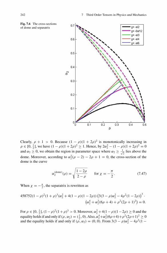
242 7 Third Order Tensors in Physics and Mechanics
Fig. 7.6 The cross-sectionsof dome and separatrix
Clearly, ρ + 1 > 0. Because (1 − ρ)(1 + 2ρ)2 is monotonically increasing inρ ∈ [0, 1
2 ], we have (1 − ρ)(1 + 2ρ)2 ≥ 1. Hence, by 2α22 − (1 − ρ)(1 + 2ρ)2 = 0
and α2 ≥ 0, we obtain the region in parameter space where α2 ≥ 1√2
lies above the
dome. Moreover, according to α22(ρ − 2) − 2ρ + 1 = 0, the cross-section of the
dome is the curve
α(dome)2 (ρ) =
√1 − 2ρ
2 − ρfor χ = −π
2. (7.47)
When χ = −π2 , the separatrix is rewritten as
458752(1 − ρ)2(1 + ρ)3(α22 + 4(1 − ρ)(1 − 2ρ))
(3(3 − ρ)α2
2 − 4ρ2(1 − 2ρ))3 ·
(α4
2 + α22(6ρ + 4) + ρ2(2ρ + 1)2
) = 0.
For ρ ∈ [0, 12 ], (1 −ρ)2(1 +ρ)3 > 0. Moreover, α2
2 + 4(1 −ρ)(1 − 2ρ) ≥ 0 and theequality holds if and only if (ρ, α2) = ( 1
2 , 0). Also, α42+α2
2(6ρ+4)+ρ2(2ρ+1)2 ≥ 0and the equality holds if and only if (ρ, α2) = (0, 0). From 3(3 − ρ)α2
2 − 4ρ2(1 −

7.5 Algebraic Expression of the Separatrix Surface 243
2ρ) = 0, we obtain that the cross-section of the separatrix is the curve
α(sepa)2 (ρ) = 2ρ√
3
√1 − 2ρ
3 − ρfor χ = −π
2. (7.48)
These two curves in (7.47) and (7.48) have a common vertical tangent at ρ = 12 .
Furthermore, since
[α(dome)2 (ρ)]2 − [α(sepa)
2 (ρ)]2 = (3 − 2ρ)2(1 − ρ − 2ρ2)
3(2 − ρ)(3 − ρ)≥ 0
in ρ ∈ [0, 12 ] and the equality holds if and only if ρ = 1
2 , we confirm analyticallythat the separatrix lies below the dome when χ = −π
2 .Applying a similar discussion for the case χ = −π
6 , the following curves areobtained as representations for cross-sections of the dome and separatrix, respec-tively,
α(dome)2 (ρ) = 1 − 2ρ√
2
√1 + ρ, α
(sepa)2 (ρ) = 2ρ√
3
√1 + 2ρ
3 + ρ. (7.49)
They intersect at (ρ, α2) =(
13 ,
√2
3√
3
).
7.6 Eigendiscriminant from Algebraic Geometry
At the beginning, we review the traceless property of the symmetric octupolar tensorfrom the viewpoint of harmonic functions.
Definition 7.4 Let f : U �→ R (where U is an open subset of Rn) be a twicecontinuously differentiable function. We say f is a harmonic function if it satisfiesLaplace’s equation everywhere on U :
Δ f = 0, i.e.,∂2 f
∂x21
+ ∂2 f
∂x22
+ · · · + ∂2 f
∂x2n
= 0.
Suppose that A ∈ S3,3 is an octupolar tensor, and Φ(x) = A x3 is the octupolarpotential. Using the Laplace operator, we get
ΔΦ(x) = ∂2
∂x21
Φ(x) + ∂2
∂x22
Φ(x) + ∂2
∂x23
Φ(x)
= 6 ((a111 + a122 + a133)x1 + (a112 + a112 + a233)x2 + (a113 + a223 + a333)x3)
= 0.

244 7 Third Order Tensors in Physics and Mechanics
Hence, the traceless property (7.27) holds. In this sense, we say that the traceless ofthe octupolar tensor A is annihilated by the Laplace operator.
Second, we claim that the separatrix (7.45) is indeed the eigendiscriminant ofthe octupolar tensor (7.34) [1, 256]. Before we start, let the given tensor A ∈ Tm,n
be generic, which means that A lies in a certain dense open subset in the tensorspace Tm,n . This subset will be characterized later as the nonvanishing locus of theeigendiscriminant. In algebraic geometry, the solution set of a system of polynomialequations is called a variety [19]. We now consider the system A xm−1 = λx, whichis equivalent to
rank((A xm−1 x)
) ≤ 1. (7.50)
Clearly, the E-eigenvectors of A are the solutions of the above system. The eigencon-figuration of A is the variety defined by the 2-by-2 minors of the matrix (A xm−1 x).Then, we have the following theorem.
Theorem 7.20 (Cartwright, Sturmfels 2013) Let A ∈ Sm,n be generic. The numberof solutions of the system (7.50) is
ρ(n, m) = (m − 1)n − 1
m − 2=
n−1∑
i=0
(m − 1)i .
The same count holds for eigenconfigurations of symmetric tensors.
If the tensor is not generic, then its eigenconfiguration consists of fewer thanρ(n, m) points or is not zero-dimensional. The elements of all these non-generictensors satisfy an irreducible homogeneous polynomial, called the eigendiscriminantΔn,m . The degree of the eigendiscriminant is presented in the following theorem.
Theorem 7.21 (Abo, Seigal, Sturmfels 2017) The eigendiscriminant is an irre-ducible homogeneous polynomial of degree
degree(Δn,m) = n(n − 1)(m − 1)n−1.
From this theorem, we know that the eigendiscriminant of the octupolar tensorsA (α0, β3, α2) in (7.34) is a homogeneous polynomial in variables α0, β3, α2 withdegree 24. This fact is coincide with the separatrix in (7.45).
Motivated by this result, we apply the eigendiscriminant for the octupolar ten-sors A ∈ S3,3. The corresponding octupolar potentials are ternary cubics that areharmonic. We recall that the octupolar phase of a molecule assembly of bent-coreliquid crystals has two generic states: the octupolar potential has four/three maxi-mum points on the unit sphere. An ideal octupolar phase has four maximum points.When passing through the separatrix surface, two maximum points coincide. Thatis to say, two E-/Z-eigenvalues of the octupolar tensor meet and integrate into one.This corresponds to vanishing of the eigendiscriminant.

7.7 Notes 245
7.7 Notes
The conception “tensor” was originally arising from physics and mechanics [134].Hence, it is necessary to address tensors in physics and mechanics. However, tensorsin physics and mechanics are different from hypermatrices. Specifically, let A bea third order tensor. Under a Cartesian basis {e1, e2, e3}, the components of A in{e1, e2, e3} could be represented as a hypermatrix
⎛
⎝a111 a112 a113 a211 a212 a213 a311 a312 a313
a121 a122 a123 a221 a222 a223 a321 a322 a323
a131 a132 a133 a231 a232 a233 a331 a332 a333
⎞
⎠ .
The representation of the tensor A in terms of its components can also be expressedas
A =3∑
i, j,k=1
ai jkei ⊗ e j ⊗ ek .
This representation is particularly convenient when using a general coordinate sys-tem.
Section 7.1 The difference between tensors and hypermatrices was studied by Qi[225]. Some valuable viewpoints and new notions, such as tensor transpose, kerneltensor, nonsingularity, and L-inverse of tensors, were introduced. The L-inverse ofthird order tensors is a nontrivial generalization of inverse of second order tensors.
Section 7.2 The piezoelectric effects was discovered by Curie brothers. Nowa-days, piezoelectric material as well as its piezoelectric tensor are active researcharea. Chen, Jákli and Qi [51] proposed the C-eigenvalues for piezoelectric tensors.Furthermore, Li and Li [166] gave bounds for the C-eigenvalues of piezoelectrictensors.
Section 7.3 Virga [270] studied two dimensional symmetric traceless tensors aris-ing from liquid crystals. Gaeta and Virga [99] addressed three dimensional symmetrictraceless tensors. Here, traces of each slice matrix of a traceless tensor are all zeros.This reflects an important property in physics. Some other papers on liquid crystaltensors include [24, 184, 186].
Gaeta and Virga [99] demonstrated an interesting approach for reducing indepen-dent parameters of a symmetric traceless tensor from seven to three. The expressionsof the dome and the separatrix get benefit from this approach.
Section 7.4 The existence of the dome was pointed by Gaeta and Virga [99]. Chen,Qi and Virga [52] used the E-characteristic polynomial from spectral tensor theory[221, 228] to obtain the algebraic expression of the dome.
Section 7.5 Gaeta and Virga [99] pointed out that there are two generic octupolarstates. Moreover, they gave a numerical simulation for the separatrix. Chen, Qi andVirga [52] employed resultant theory from algebraic geometry to gave a close-formsolution for the separatrix.

246 7 Third Order Tensors in Physics and Mechanics
Section 7.6 The traceless property of a tensor is due to the Laplace operator. Insimple terms, the algebraic expression of the dome was motivated by two meetingZ-eigenvalues, and the closed-form solution of the separatrix was motivated by twomeeting Z-eigenvectors. Such a viewpoint from algebraic geometry may give ussome insights to this problem.
Finally, we discuss octupolar tensors in two dimensions. We consider third ordertwo dimensional symmetric traceless tensors
A =(
a111 a112 a112 a122
a112 a122 a122 a222
)∈ S3,2. (7.51)
By using traceless property
a111 + a122 = 0 and a112 + a222 = 0,
and introducing parameters α = a111 and β = a222, we obtain
A =(
α −β −β −α
−β −α −α β
).
On the compact circle x21 + x2
2 = 1, the potential function Φ(x) = A x3 has atleast one maximum point. Without lose of generality, we assume the maximum pointbeing (1, 0)�. By writing down the KKT system A x2 = λx explicitly as
{αx2
1 − 2βx1x2 − αx22 = λx1,
−βx21 − 2αx1x2 + βx2
2 = λx2,
we get (1, 0)� satisfying the above system and obtain
β = 0.
Hence, the octupolar tensor
A =(
α 0 0 −α
0 −α −α 0
)
has only one parameter α.Without loss of generality, we only need to consider the constant tensor
A =(
1 0 0 −10 −1 −1 0
).
Its E-characteristic polynomial is
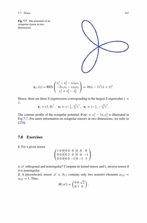
7.7 Notes 247
Fig. 7.7 The potential of anoctupolar tensor in twodimensions
φA (λ) = RES
⎛
⎝x2
1 − x22 − λx0x1
−2x1x2 − λx0x2
x21 + x2
2 − x20
⎞
⎠ = 16(λ − 1)3(λ + 1)3.
Hence, there are three Z-eigenvectors corresponding to the largest Z-eigenvalue λ =1:
x1 = (1, 0)�, x2 = (− 12 ,
√3
2 )�, x2 = (− 12 ,−
√3
2 )�.
The contour profile of the octupolar potential Φ(x) = x31 − 3x1x2
2 is illustrated inFig. 7.7. For more information on octupolar tensors in two dimensions, we refer to[270].
7.8 Exercises
1. For a given tensor ⎛
⎝1 0 0 0 0 0 0 0 00 0 0 0 2 0 0 0 −10 0 0 0 0 −1 0 −1 3
⎞
⎠ ,
is A orthogonal and nonsingular? Compute its kernel tensor and L-inverse tensor ifit is nonsingular.2. A piezoelectric tensor A ∈ S3,2 contains only two nonzero elements a112 =a222 = 1. Thus,
M(A ) =(
0 0√
20 1 0
).
248 7 Third Order Tensors in Physics and Mechanics
Compute the largest singular value of M(A ) and the largest C-eigenvalue of A , andcompare them.3. For the tensor A (α) with α > 0 in Proposition 7.6: a123 = a213 = a312 = −α andother elements of A (α) are all zeros, prove that the largest C-eigenvalue of A (α) is
2√3α.
4. Compute positive Z-eigenvalues and associated Z-eigenvectors of A (0,− 12 ,
√2
2 )
and A (0,−1, 0), where A (α0, β3, α2) is defined in (7.34).5. When χ = −π
6 in the polar coordinates (7.46), prove that the algebraic expressionsof the dome and separatrix curves are (7.49).
Chapter 8Fourth Order Tensors in Physics andMechanics
Fourth order tensors have also wide applications in physics and mechanics. Examplesinclude the piezo-optical tensor, the elasto-optical tensor and the flexoelectric tensor.The most well-known fourth order tensor is the elasticity tensor [134, 212, 318]. Itis closely related to the strong ellipticity condition in nonlinear mechanics.
The strong ellipticity condition plays an important role in nonlinear elasticity andin materials. In this chapter, we will discuss the application of the spectral theory oftensors to the studying of strong ellipticity of elasticity.
First of all, we will define M-eigenvalues for an elasticity tensor. It will be shownthat the strong ellipticity condition holds if and only if the smallest M-eigenvalue ofthe elasticity tensor is positive. We will say that the elasticity tensor is M-positivedefinite (M-PD) if the strong ellipticity condition holds. We will also define S-positivedefiniteness for the elasticity tensor. The elasticity tensor is S-positive definite (S-PD)if its unfolded symmetric matrix is positive definite. If the elasticity tensor is S-PD,then the strong ellipticity condition holds. The converse conclusion is not right. Itis easy to check the elasticity tensor is S-PD or not, as this only needs to check ifthe smallest eigenvalue of the unfolding matrix of the elasticity tensor is positiveor not. Thus, S-positive definiteness provides a checkable sufficient condition forstrong ellipticity.
Then, we will derive necessary and sufficient conditions for the strong ellipticitycondition of anisotropic elastic materials. It can be observed that the strong ellipticitycondition holds if and only if a second order tensor function is positive definite for anyunit vectors. Then one can further link this condition to positive definiteness of threesecond-order symmetric tensors, a fourth order symmetric tensor and a sixth-ordersymmetric tensor. In particular, we will consider conditions of strong ellipticity of therhombic classes, for which one needs to check the co-positivity of three second-ordersymmetric tensors and the positive definiteness of a sixth-order symmetric tensor.One may check this necessary and sufficient condition by computing the smallestZ-eigenvalues of these symmetric tensors via the method of Cui, Dai and Nie [66].
© Springer Nature Singapore Pte Ltd. 2018L. Qi et al., Tensor Eigenvalues and Their Applications, Advances in Mechanicsand Mathematics 39, https://doi.org/10.1007/978-981-10-8058-6_8
249

250 8 Fourth Order Tensors in Physics and Mechanics
Thus, numerically, this provides a practical method for checking the strong ellipticitycondition of a given elasticity tensor.
Since the range of S-positive (semi)definiteness is too narrow, to extend the cov-erage of S-PSD tensors, then we will study several sufficient conditions for strongellipticity, other than S-positive definiteness. An alternating algorithm for check-ing this sufficient condition is described. Some other sufficient conditions are alsodiscussed. Furthermore, we define elasticity M-tensors and nonsingular elasticityM-tensors. If the elasticity M-tensor is a nonsingular elasticity M-tensor, then thestrong ellipticity condition holds. We give an example to show that a nonsingularelasticity M-tensor may not be S-PD. We then present a sufficient condition whichsays that the strong ellipticity holds if unfolding matrix can be modified to a positivedefinite one by preserving the summation of some entries.
We also study strong ellipticity for higher order elasticity tensors. Paired sym-metric tensors and strongly paired symmetric tensors are defined. It is easy to knowthat all fourth order three dimensional elasticity tensors are paired symmetric ten-sors. The notion of M-eigenvalue for elasticity tensors is generalized for sixth orderpaired symmetric tensors as well as the strong ellipticity. In addition, we study con-ditions under which the paired symmetric tensor is M-positive semidefiniteness orM-positive definiteness. At last, a sequential semidefinite programming method isproposed by using semidefinite relaxation technique.
8.1 The Elasticity Tensor, Strong Ellipticity andM-Eigenvalues
Hooke’s law, named after 17th-century British physicist Robert Hooke (1635–1703),is a principle of physics that the force needed to extend or compress a spring by somedistance is proportional to that distance. The modern theory of elasticity generalizesHooke’s law to say that the strain (deformation) tensor S = (Si j ) (a second order threedimensional symmetric tensor) of an elastic object or material is the tensor productof the elasticity tensor (a fourth order tensor) C = (Ci jkl) and the stress tensorE = (Ekl) (another second order three dimensional symmetric tensor) applied tothat elastic object or material, i.e.,
Si j =3∑
k,l=1
Ci jkl Ekl .
Since S and E are symmetric, C is symmetric with respect to the first two indices iand j , and the last two indices k and l, respectively, i.e.,
Ci jkl = C jikl = Ci jlk,

8.1 The Elasticity Tensor, Strong Ellipticity and M-Eigenvalues 251
for i, j, k, l = 1, 2, 3. This is called minor symmetry in the mechanics literature.Furthermore, the elasticity tensor C has a major symmetry, i.e.,
Ci jkl = Ckli j ,
for i, j, k, l = 1, 2, 3. Thus, the elasticity tensor has 21 independent entries, whichare called elasticities.
Elasticities are related to elastic moduli. Depending upon how stress and strain areto be measured, including directions, there are various types of elastic moduli. Thethree primary ones are Young’s modulus, the shear modulus or modulus of rigidity,and the bulk modulus. Three other elastic moduli are Poisson’s ratio, Lamé’s firstparameter, and P-wave modulus.
An important topic in elasticity theory is the strong ellipticity condition whichguarantees the existence of solutions of basic boundary-value problems of elasto-statics and thus ensures an elastic material to satisfy some mechanical properties.Research works on this topic include Knowles and Sternberg [158, 159], Simpsonand Spector [244], Rosakis [236], Wang and Aron [276], Walton and Wilber [271],Chirita, Danescu, and Ciarletta [59], Zubov and Rudev [319], and Gourgiotis andBigoni [106], etc.
We now use A = (ai jkl) to denote the elasticity tensor of some elastic material.By the discussion at the beginning of this section, it satisfies the following symmetry:
ai jkl = a jikl = ai jlk = akli j . (8.1)
And the strong (ordinary) ellipticity condition holds if
f (x, y) = A xyxy =n∑
i, j,k,l=1
ai jkl xi y j xk yl > 0(≥ 0)
for all unit vectors x, y ∈ Rn . According to Knowles and Sternberg [158, 159], theterm “strong ellipticity condition” is a common usage in mechanics.
Now, for a given elasticity tensor A = (ai jkl), we define another fourth ordertensor ¯A = (ai jkl) with entries satisfying
ai jkl = ai jkl + ak jil + ailk j + akli j
4, for i, j, k, l ∈ [n].
So, the new tensor ¯A satisfies
ai jkl = ak jil = akli j , (8.2)
and it is obvious that
A xyxy = ¯A xyxy, for any x, y ∈ Rn.

252 8 Fourth Order Tensors in Physics and Mechanics
In the following analysis, we always consider the fourth order tensors with symmetry(8.2). Denote E4,n the set containing all fourth order n dimensional tensors satisfying(8.2). We mainly consider the cases n = 2 or n = 3 in this section.
By optimization theory, we may see that the strong ellipticity condition holdsif and only if the optimal value of the following optimization problem is positive,and the ordinary ellipticity condition holds if and only if the optimal value of thisoptimization problem is nonnegative.
min A xyxys.t. x�x = 1, y�y = 1.
(8.3)
Based this observation, we introduce the definition of M-eigenvalues for fourth ordern-dimensional tensors which satisfy (8.2).
Definition 8.1 Let A = (ai jkl) ∈ E4,n , i, j, k, l ∈ [n], where n = 3. If there areλ ∈ R, x, y ∈ Rn\{0} satisfying that
⎧⎪⎪⎪⎪⎨
⎪⎪⎪⎪⎩
A · yxy = λx,
A xyx· = λy,
x�x = 1,
y�y = 1,
(8.4)
where A · yxy, A xyx· are vectors whose i th components are
n∑
j,k,l=1
ai jkl y j xk yl andn∑
i, j,k=1
ai jkl xi y j xk,
then we call λ an M-eigenvalue of A , and call x, y left and right M-eigenvectors ofA , associated with the M-eigenvalue λ.
Here, “M” means mechanics. We now have the following result.
Theorem 8.1 Let A ∈ E4,n. Then its M-eigenvalue always exists. Let x, y be left andright M-eigenvectors of A , associated with an M-eigenvalue λ. Then λ = A xyxy.Furthermore, the strong ellipticity condition holds if and only if the smallest M-eigenvalue of A is positive, and the ordinary ellipticity condition holds if and onlyif the smallest M-eigenvalue of A is nonnegative.
Proof For the optimization problem (8.3), it is obvious that the problem has at leastone maximizer and one minimizer since the objective function is continuous andits feasible region is compact. By the optimality conditions of problem (8.3), thereare λ ∈ R, x, y ∈ Rn\{0} such that (8.4) holds, which implies that M-eigenvaluesalways exist, and it is not difficult to see that
λ = A xyxy.
Then the other results follow this directly. �

8.1 The Elasticity Tensor, Strong Ellipticity and M-Eigenvalues 253
Thus, for any elasticity tensor A ∈ E4,n satisfying (8.2), if the strong ellipticitycondition holds, we also say that A is M-positive definite (M-PD), and if the ordinaryellipticity condition holds, we also say that A is M-positive semi-definite (MPSD).
In the following analysis, denote λA as the M-eigenvalue of tensor A with thelargest absolute value. For λ ∈ R, we say λxyxy = λx ⊗ y ⊗ x ⊗ y is the bestrank-one approximation of A , if it can minimize ‖A − λxyxy‖F , where the norm‖ · ‖F is the Frobenius norm, and x�x = 1, y�y = 1. The next theorem provides anapplication of the M-eigenvalue in the best rank-one approximation for fourth orderthree dimensional tensors satisfying (8.2).
Theorem 8.2 Let A ∈ E4,n. Let x, y be left and right M-eigenvectors of A , asso-ciated with λA . Then, λA xyxy is the best rank-one approximation of A .
Proof Let λ ∈ R be any scalar. Suppose x ∈ Rm, y ∈ Rn such that x�x = 1, y�y =1. Then, we know that
‖A − λxyxy‖2F =‖A ‖2
F − 2λA xyxy + λ2(x�x)(y�y)
=‖A ‖2F − 2λA xyxy + λ2.
It is obvious that the minimum of ‖A − λxyxy‖ must be attained at λ = A xyxy.Thus, it holds that
min{‖A − λxyxy‖2F | λ ∈ R, x�x = 1, y�y = 1}
= min{‖A ‖2F − (A xyxy)2 | x�x = 1, y�y = 1}
= ‖A ‖2F − max{(A xyxy)2 | x�x = 1, y�y = 1},
and the desired result holds. �
Let P = (pii ′) ∈ Rm×m and Q = (q j j ′) ∈ Rn×n be two orthogonal matrices.Suppose tensor B = (bi jkl) is defined such that
bi jkl =m∑
i ′,k ′=1
n∑
j ′,l ′=1
pii ′q j j ′ pkk ′qll ′ai ′ j ′k ′l ′ .
Then we say A ∈ E4,n and B are orthogonally similar. It is not difficult to see thatif A satisfies the partially symmetric condition (8.2), then B also satisfies (8.2).The following conclusion holds, and the proof is omitted since it can be proved bydefinition directly.
Theorem 8.3 Let A ∈ E4,3. Assume B is another fourth order three dimensionaltensor orthogonal similar to A via orthogonal matrices P and Q. Then the followingresults hold:
(1) A and B have the same M-eigenvalues;
254 8 Fourth Order Tensors in Physics and Mechanics
(2) if λ is an M-eigenvalue of A with left and right M-eigenvectors x and y, then λ
is also an M-eigenvalue of B with left and right M-eigenvectors Px and Qy.
Theorems 8.1 and 8.3 reveal that the M-eigenvalues are some intrinsic parametersof the elasticity tensor. Recently, Xiang, Qi and Wei [289] showed that there aretwo M-eigenvalues in the isotopic case. The first M-eigenvalue is the shear modulusG, and must be positive. The second M-eigenvalue is the P-wave modulus. Hence,in the isotropic case, strong ellipticity holds if and only if the P-wave modulus ispositive. Xiang, Qi and Wei [289] further showed that the positiveness condition ofthe M-eigenvalues coincides with the existing conditions for strong ellipticity in thecubic case and the polar anisotropic case. This further reveals the physical meaningsof M-eigenvalues and indicates that the positiveness condition of M-eigenvalues ismore general for strong ellipticity.
We now define S-positive definiteness for elasticity tensors A ∈ E4,n . Suchproperty has been considered by Lord Kelvin 160 years ago [261, 262]. Let A =(ai jkl) ∈ E4,n be an elasticity tensor satisfying (8.2). We say that A is S-positivedefinite (S-PD) if
A D2 =n∑
i, j,k,l=1
ai jkldi j dkl > 0
for all D = (di j ) ∈ Rn×n . Similarly, we say that A is S-positive semi-definite(S-PSD) if
A D2 =n∑
i, j,k,l=1
ai jkldi j dkl ≥ 0
for all D = (di j ) ∈ Rn×n . For any x, y ∈ Rn , we can define di j = xi y j . Thisimplies that the S-positive definiteness is a sufficient condition for the M-positivedefiniteness. The following example shows that the converse is not true.
Let A = (ai jkl) ∈ E4,2 be an elasticity tensor satisfying (8.2). Its independententries are defined as
a1111 = 1, a1112 = 2, a1122 = 4, a1212 = 12, a2121 = 12,
a1222 = 1, a1121 = 2, a2122 = 1, a2222 = 2.
Then, the corresponding homogeneous polynomial can be written as
f (x, y) = A xyxy
= x21 y2
1 + 4x21 y1 y2 + 12x2
1 y22 + 4x1x2 y2
1 + 16x1x2 y1 y2
+ 2x1x2 y22 + 12x2
2 y21 + 2x2
2 y1 y2 + 2x22 y2
2 .
By a direct computation, we can find its smallest M-eigenvalue λ = 0.5837. Thus,the tensor A is M-PD. On the other hand, to discuss its S-positive definiteness, we
8.1 The Elasticity Tensor, Strong Ellipticity and M-Eigenvalues 255
can rewrite the matrix D ∈ Rn×n to an n2-dimensional vector, and A can be rewrittenas a symmetric matrix in Rn2×n2
. Then, it holds that A is S-PD if and only if thecorresponding symmetric matrix is positive definite. For this example, n = 2, the4 × 4 symmetric matrix is
⎛
⎜⎜⎝
a1111 a1112 a1121 a1122
a1112 a1212 a1122 a1222
a1121 a1222 a2121 a2122
a1122 a1122 a2122 a2222
⎞
⎟⎟⎠ =
⎛
⎜⎜⎝
1 2 2 42 12 4 12 4 12 14 1 1 2
⎞
⎟⎟⎠ .
Since the smallest eigenvalue of this symmetric matrix is −2.6110 < 0, we concludethat A is not S-PD. Thus, S-positive definiteness is a sufficient but not necessarycondition for M-positive definiteness.
We use the name “S-positive definiteness” as this is related with S-eigenvalues offourth order tensors defined in [228], where the eigenvalues of the n × n unfoldedsymmetric matrix described above are called the S-eigenvalues of the tensor A .
To end this section, we describe a direct method for computing M-eigenvalues offourth order two dimensional tensors satisfying (8.2) i.e. tensors such that A ∈ E4,n
and n = 2. The key technique is the Sylvester formula of the resultant, which is usedto solve a system involving only two variables. In fact, by Definition 8.1, we canalways homogenize the first two equations of (8.4) by the following form
{A · yxy = λ(y�y)x,
A xyx· = λ(x�x)y(8.5)
According to the resultant theory [64], we know that (8.5) has a nonzero complexsolution (x, y) if and only if λ is a root of the resultant. Particularly, for the casen = 2, the following results hold.
Theorem 8.4 Let A = (ai jkl) ∈ E4,n with n = 2. Then the following results holdfor its M-eigenvalues and the corresponding M-eigenvectors:
(1) if a1112 = a1121 = 0, then λ = a1111 is an M-eigenvalue of A and the corre-sponding left and right M-eigenvector is x = y = (1, 0)�;
(2) for any real roots (u, v)� of the following equations
{a1121u2 + (a2121 − a1111)uv − a1121v2 = 0,
a1112u2 + 2a1122uv + a2122v2 = 0,(8.6)
it holds that λ = a1111u2 + 2a1121uv + a2121v2 is an M-eigenvalue with the leftand right M-eigenvector such that
x = (u, v)�√u2 + v2
, y = (±1, 0);

256 8 Fourth Order Tensors in Physics and Mechanics
(3) for any real roots (u, v)� of the following equations
{a1121u2 + 2a1122uv + a1222v2 = 0,
a1112u2 + (a1212 − a1111)uv − a1112v2 = 0,(8.7)
it holds that λ = a1111u2 + 2a1112uv + a1212v2 is an M-eigenvalue with the leftand right M-eigenvectors such that
x = (±1, 0)�, y = (u, v)�√u2 + v2
;
(4) λ = A xyxy is an M-eigenvalue with left and right M-eigenvectors such that
x = ± (u, 1)�√u2 + 1
, y = ± (v, 1)�√v2 + 1
.
Furthermore, u, v are real solutions of the following system of polynomial equa-tions
⎧⎪⎪⎪⎪⎨
⎪⎪⎪⎪⎩
a1121u2v2 + 2a1122u2v + a1222u2 + (a2121 − a1111)uv2 − a1121v2
+ 2(a2122 − a1112)uv + (a2222 − a1212)u − 2a1122v − a1222 = 0,
a1112u2v2 + (a1212 − a1111)u2v − a1112u2 + 2(a1222 − a1121)uv
+ 2a1122uv2 − 2a1122u + a2122v2 + (a2222 − a2121)v − a2122 = 0.
Moreover, if a1112 = a1121 = 0, all M-eigenvalues and related M-eigenvectors ofA are given by (1)–(4); otherwise, they are given by (2)–(4).
Proof (1) If a1112 = a1121 = 0, according to Definition 8.1, by a direct computationthat (1) holds.
(2) If y2 = 0, then y1 = 1 or y1 = −1, by Definition 8.1, we have
⎧⎪⎪⎪⎪⎪⎪⎨
⎪⎪⎪⎪⎪⎪⎩
a1111x1 + a1121x2 = λx1,
a2111x1 + a2121x2 = λx2,
a1111x21 + 2a1121x1x2 + a2121x2
2 = λ,
a1112x21 + 2a1122x1x2 + a2122x2
2 = 0,
x21 + x2
2 = 1.
By the first two equations, we have
⎧⎪⎨
⎪⎩
a1121x21 + (a2121 − a1111)x1x2 − a1121x2
2 = 0,
a1112x21 + 2a1122x1x2 + a2122x2
2 = 0,
x21 + x2
2 = 1.
8.1 The Elasticity Tensor, Strong Ellipticity and M-Eigenvalues 257
Suppose u = x1√x2
1 +x22
, v = x2√x2
1 +x22
, the desired result (2) holds.
(3) We can prove this by a similar way as (2).(4) If x2 = 0 and y2 = 0, by (8.4), it follows that
⎧⎪⎪⎪⎪⎪⎪⎪⎪⎪⎪⎪⎪⎪⎪⎪⎪⎪⎪⎪⎪⎨
⎪⎪⎪⎪⎪⎪⎪⎪⎪⎪⎪⎪⎪⎪⎪⎪⎪⎪⎪⎪⎩
a1111x1 y21 + 2a1112x1 y1 y2 + a1212x1 y2
2 + a1121x2 y21
+ 2a1122x2 y1 y2 + a1222x2 y22 = λx1,
a1121x1 y21 + 2a1122x1 y1 y2 + a1222x1 y2
2 + a2121x2 y21
+ 2a2122x2 y1 y2 + a2222x2 y22 = λx2,
a1111x21 y1 + a1112x2
1 y2 + 2a1121x1x2 y1 + 2a1122x1x2 y2
+ a2121x22 y1 + a2122x2
2 y2 = λy1,
a1112x21 y1 + a1212x2
1 y2 + 2a1122x1x2 y1 + 2a1222x1x2 y2
+ a2122x22 y1 + a2222x2
2 y2 = λy2,
x21 + x2
2 = 1,
y21 + y2
2 = 1.
(8.8)
Denote u = x1x2
and v = y1
y2. By the first two equations of (8.8), it holds that
a1121u2v2 + 2a1122u2v + a1222u2 + (a2121 − a1111)uv2 − a1121v2
+ 2(a2122 − a1112)uv + (a2222 − a1212)u − 2a1122v − a1222 = 0.(8.9)
From the third equation and the fourth equation of (8.8), it follows that
a1112u2v2 + (a1212 − a1111)u2v − a1112u2 + 2(a1222 − a1121)uv
+ 2a1122uv2 − 2a1122u + a2122v2 + (a2222 − a2121)v − a2122 = 0.(8.10)
Combining (8.9) and (8.10) and the fact that x21 + x2
2 = 1, y21 + y2
2 = 1, the desiredresults hold automatically. �
8.2 Strong Ellipticity via Z-Eigenvalues of SymmetricTensors
In the last section, we studied the strong ellipticity condition for the elasticity tensorfor isotropic materials. Several sufficient conditions for preserving the strong ellip-ticity condition were given. Now, we study some necessary and sufficient conditionsfor the strong ellipticity condition. The main tool for this study is Z-eigenvaluesof symmetric tensors. Particularly, the strong ellipticity condition of the elasticitytensor can be connected with the smallest Z-eigenvalue of some symmetric tensors.

258 8 Fourth Order Tensors in Physics and Mechanics
For both planar and three dimensional cases, checkable conditions are given to findall Z-eigenvalues of any tensor with even order.
The other tool that will be used to establish the necessary and sufficient conditionfor the strong ellipticity condition of the elasticity tensor is the strict copositivity ofa second-order symmetric tensor. To move on, we first cite a useful lemma.
Lemma 8.1 (Simpson, Spector 1983) Suppose M = (mi j ) ∈ R3×3 is a symmetricmatrix. Then, M is strictly copositive if and only if the following conditions hold:
m11 > 0, m22 > 0, m33 > 0,
R ≡ m12 + (m11m22)12 > 0, S ≡ m13 + (m11m33)
12 > 0,
T ≡ m23 + (m22m33)12 > 0,
m1233m12 + m
1222m13 + m
1211m23 + (2RST )
12 + (m11m22m33)
12 > 0.
In Theorem 8.4, we studied a method to compute all the M-eigenvalues of theelasticity tensor for n = 2. Now, we study the case that n = 3.
Suppose A = (ai jkl) is the elasticity tensor with i, j, k, l ∈ [3]. Here, [3] standsfor a set {1, 2, 3}. Let Q(x) = (q jl) ∈ R3×3 denote the acoustic tensor, which isdefined by
q jl =3∑
i,k=1
ai jkl xi xk . (8.11)
Then Q(x) is a second-order symmetric tensor. By the analysis of the last section, thetensor A is M-PD or the strong ellipticity condition holds if and only if the acoustictensor Q(x) is positive definite for all unit vector x. As we all know that a symmetricmatrix is positive definite if and only if all of its leading principal minors are positivedefinite. For the sake of simplicity, we define the following matrices:
M1 =⎛
⎝a1111 a1121 a1131
a1121 a2121 a2131
a1131 a2131 a3131
⎞
⎠ , M2 =⎛
⎝a1212 a1222 a1232
a1222 a2222 a2232
a1232 a2232 a3232
⎞
⎠ , (8.12)
and
M3 =⎛
⎝a1313 a1323 a1333
a1323 a2323 a2333
a1333 a2333 a3333
⎞
⎠ . (8.13)
We now consider the diagonal entries of Q(x). By (8.11), it holds that
q11 = a1111x21 + 2a1121x1x2 + 2a1131x1x3 + a2121x2
2 + 2a2131x2x3 + a3131x23 ,
q22 = a1212x21 + 2a1222x1x2 + 2a1232x1x3 + a2222x2
2 + 2a2232x2x3 + a3232x23 ,
q33 = a1313x21 + 2a1323x1x2 + 2a1333x1x3 + a2323x2
2 + 2a2333x2x3 + a3333x23 .
(8.14)

8.2 Strong Ellipticity via Z-Eigenvalues of Symmetric Tensors 259
From (8.12)–(8.14), its obvious that
q11 > 0, ∀ x = 0 ⇔ M1 is positive definite ,
q22 > 0, ∀ x = 0 ⇔ M2 is positive definite ,
q33 > 0, ∀ x = 0 ⇔ M3 is positive definite .
For all principal second-order minors of Q(x), it is not difficult to see that
q11q22 − q212, q11q33 − q2
13, q22q33 − q223
are all fourth order homogeneous polynomials corresponding to x. Suppose T , is afourth order three dimensional symmetric tensors such that
T x4 = q11q22 − q212,
By Theorem 1.2 in Chap. 1, we know that the second-order leading principal minorsis positive if and only if the smallest Z-eigenvalue of the fourth order tensor T ispositive.
Similar to the discussion above, let W be a sixth-order three dimensional tensorsuch that
W x4 =3∑
i1,...,i6=1
wi1...i6 xi1 xi2 . . . xi6 = det (Q(x)),
which implies that det (Q(x)) > 0 if and only if the smallest Z-eigenvalue of W ispositive. In summary, we have the following conclusion. Here, the positive definite-ness of a symmetric tensor is defined in Chap. 1.
Theorem 8.5 The strong ellipticity condition holds for the elasticity tensor A if andonly if the following three conditions hold:
(1) the symmetric matrices Mi , i ∈ [3] are positive definite;(2) the fourth order symmetric tensor T is positive definite;(3) the sixth order symmetric tensor W is positive definite.
Based on Theorem 8.5, we now discuss a kind of practical elasticity tensors fromthe rhombic system, where A = (ai jkl) satisfies the symmetries
ai jkl = akli j = ai jlk, ∀ i, j, k, l ∈ [3]. (8.15)
As stated in [59], the elasticity tensor A has entries such that
a1123 = a1131 = a1112 = a2223 = a2231 = a2212 = 0,
a3323 = a3331 = a3312 = a2331 = a2312 = a3112 = 0.(8.16)
And the nonzero components are denoted shortly by

260 8 Fourth Order Tensors in Physics and Mechanics
a11 = a1111, a22 = a2222, a33 = a3333, a12 = a1122, a23 = a2233,
a31 = a3311, a44 = a2323, a55 = a1313, a66 = a1212.
To discuss its strong ellipticity condition, the following matrices are needed:
P =⎛
⎜⎝a11a66
a11a22+a212−2a12a66
2a11a44+a55a66
2a11a22+a2
12−2a12a66
2 a22a66a44a66+a22a55
2a11a44+a55a66
2a44a66+a22a55
2 a44a55
⎞
⎟⎠ , (8.17)
Furthermore, suppose the second order symmetric tensor Q(x) and the correspondingsixth order tensor W are defined as in Theorem 8.5. The following theorem showsthe strong ellipticity for the rhombic system.
Theorem 8.6 Suppose that A is the elasticity tensor with entries satisfying (8.16).Then the strong ellipticity condition holds for A if and only if the following threeconditions hold:
(1) aii > 0 for all i ∈ [6];(2) the symmetric matrix P defined in (8.17) is copositive;(3) the sixth order symmetric tensor W is positive definite.
Proof Combining (8.14) with (8.15), we know that
q11 = a11x21 + a66x2
2 + a55x23 , q22 = a66x2
1 + a22x22 + a44x2
3 ,
q33 = a55x21 + a44x2
2 + a33x23 .
Together with (8.12) and (8.13), we obtain
M1 =⎛
⎝a11 0 00 a66 00 0 a55
⎞
⎠ , M2 =⎛
⎝a66 0 00 a22 00 0 a44
⎞
⎠ , M3 =⎛
⎝a55 0 00 a44 00 0 a33
⎞
⎠ .
Thus, from (1) of Theorem 8.5 with (8.14), we know that aii > 0 for all i ∈ [6].On the other hand, by (8.11) and (8.15)–(8.16), it is easy to know that
q11q22 − q212 = a11a66x4
1 + a11a22x21 x2
2 + a11a44x21 x2
3
+ a266x2
1 x22 + a66a22x4
2 + a66a44x22 x2
3
+ a55a66x23 x2
1 + a55a22x23 x2
2 + a55a44x43
− a212x2
1 x22 − a2
66x21x2
2 − 2a12a66x21 x2
2
= a11a66x41 + a66a22x4
2 + a55a44x43
+ (a11a22 − a212 − 2a12a66)x2
1 x22
+ (a11a44 + a55a66)x21 x2
3 + (a66a44 + a55a22)x22 x2
3
= (x21 , x2
2 , x23 )P(x2
1 , x22 , x2
3 )�, ∀ x ∈ R3\{0},
8.2 Strong Ellipticity via Z-Eigenvalues of Symmetric Tensors 261
By (2) and (3) of Theorem 8.5, we know that the desired results hold. �
It should be noted that the key part of the necessary and sufficient condition inTheorem 8.5 is to find the smallest Z-eigenvalues of the symmetric tensors T andW . Cui, Dai and Nie [66] has proposed an efficient method for computing all theZ-eigenvalues of symmetric tensors of low orders and dimensions. A package oftheir method is available via the following link:
AReigSTensors: http://www.math.ucsd.edu/njw/CODES/reigsymtensor/areigstsrweb.html
Note that the order of T is 4, the order of W is 6, and their dimensions are 3,one may use the package of Cui, Dai and Nie [66] to find the smallest Z-eigenvaluesof the symmetric tensors T and W . Thus, numerically, Theorem 8.5 provides anefficient way to determine strong ellipticity of the elasticity tensor of a material.
8.3 Other Sufficient Condition for Strong Ellipticity
In Sect. 8.1, we learned that a sufficient condition for the strong ellipticity conditionis that the elasticity tensor is S-PD. The elasticity tensor is S-PD if the unfoldedsymmetric matrix is positive definite. It is easy to check a symmetric matrix ispositive definite or not. Thus, this provides an easily checkable condition for thestrong ellipticity condition. Unfortunately, the range of the tensors satisfying S-positive definiteness are too narrow. Therefore, it is important to find some kindsof tensors that satisfy M-positive definiteness but not S-positive definiteness. In thissection, we first study another sufficient condition for strong ellipticity, and present analternating projection method to verify whether the given elasticity tensor satisfiesthis sufficient condition or not. Then we study properties of elasticity M-tensors,which is a big class of structured tensors satisfying the strong ellipticity condition,but do not satisfy S-positive definiteness. All the results here were originally studiedby Ding, Qi and Yan [85], and Ding, Liu, Qi and Yan [79] very recently.
Since the strong ellipticity condition holds for A ∈ E4,3 if and only if
f (x, y) = A xyxy :=3∑
i, j,k,l=1
ai jkl xi y j xk yl > 0, for x, y ∈ R3\{0}.
We recall that A is M-positive semidefinite if A xyxy ≥ 0 holds in the aboveequation, and A is S-positive definite (S-positive semi-definite) if
A D2 =3∑
i, j,k,l=1
ai jkldi j dkl > 0(≥ 0), ∀ D ∈ R3×3, D = 0 (D ∈ R3×3).
On the other hand, let matrix A jl = (ai jkl) ∈ R3×3 and d j = (di j ) ∈ R3 for eachi, k ∈ [3]. Then the tensor A and matrix D can be unfolded such that

262 8 Fourth Order Tensors in Physics and Mechanics
A =⎛
⎝A11 A12 A13
A21 A22 A23
A31 A32 A33
⎞
⎠ ∈ R9×9, d =⎛
⎜⎝d1
d2
d3
⎞
⎟⎠ ∈ R9. (8.18)
It is not difficult to verify that A is S-positive definite (or semidefinite respectively)if and only if the matrix A is positive definite (or semidefinite respectively), whichis a sufficient condition for the strong ellipticity of elasticity tensors as discussed inSect. 8.1.
On the other hand, for any A ∈ E4,3 and y ∈ R3, similar to the discussion inSect. 8.1, define
A y2 ∈ R3×3 with (A y2)ik =3∑
j,l=1
ai jkl y j yl ,
A x2 ∈ R3×3 with (A x2) jl =3∑
i,k=1
ai jkl xi xk .
Then it holds that A xyxy = x�(A y2)x = y�(A x2)y. By matrix theory, we knowthat every positive definite matrix can be factorized into the sum of several rank-onematrices and the minimal number of the rank-one matrices is exactly its rank. Hencethe elasticity tensor A ∈ E4,3 is M-PSD if
A y2 =r∑
s=1
αs(Usy)(Usy)�, αs > 0, (8.19)
where Us ∈ R3×3, s ∈ [r ]. Apparently, we know that r ≥ 3 if A is M-PD. Withoutloss of generality, suppose Us = (u(s)
ik ) ∈ R3, s ∈ [r ]. By (8.19), it follows that
(A y2)ik =3∑
j,l=1
ai jkl y j yl
=r∑
s=1
αs
⎛
⎝3∑
j=1
u(s)i j y j
⎞
⎠(
(3)∑
l=1
uskl yl
)
=3∑
j,l=1
(r∑
s=1
αsu(s)i j u(s)
kl
)y j yl ,
which implies that given Us , the entries of A are uniquely determined by
ai jkl = 1
2
r∑
s=1
αs(u(s)i j u(s)
kl + u(s)k j u(s)
il ). (8.20)
8.3 Other Sufficient Condition for Strong Ellipticity 263
Then we need to consider when the tensor A can be written as (8.20). By (8.19), letB = (bi jkl), i, j, k, l ∈ [3] be defined by
bi jkl =r∑
s=1
αsu(s)i j u(s)
kl .
It is easy to check that bi jkl = bkli j but B may not obey the partial symmetrycondition (8.2). Moreover, similar to (8.18), we know that the unfolding matrix B ofB is positive semidefinite such that
B =r∑
s=1
αsusu�s ,
where us ∈ R9 is the unfolding vector of Us, s ∈ [r ]. Therefore, we know that B isS-PSD since αs > 0, s ∈ [r ]. By a direct computation, we obtain that
ai jkl = akiil = 1
2(bi jkl + bk jil), ∀ i, j, k, l ∈ [3],
which implies thatA xyxy = Bxyxy = B(xy�)2.
Hence, A is M-PD or M-PSD if B is S-PD or S-PSD. We now define two new tensorsets such that
TA := {T : ti jkl = tkli j , ti jkl + tkli j = 2ai jkl},
S := {T : ti jkl = tkli j ,T is S-PSD}.
Then we have the following result.
Theorem 8.7 Suppose A ∈ E4,3, the following results hold:
(1) if TA ∩ S = ∅, then A is M-positive semi-definite;(2) if TA ∩ (S\∂S) = ∅, then A is M-positive definite.
In addition, an alternating projection method is proposed in [85] to check whetherthe intersection of two closed convex sets is empty or not. Assume P1 and P2 areprojection operators onto TA and S respectively such that
{Bt+1 = P2(A
t ),
A t+1 = P1(Bt+1),
t = 0, 1, 2, · · · .
Here, for any given tensor A ∈ E4,3, we can take A 0 = A . So the mainly iterativeprocess can be defined such that

264 8 Fourth Order Tensors in Physics and Mechanics
Algorithm 8.1 For given tensor A ∈ E4,3, set A 0 = A . Let A(t) and B(t) be theunfolding matrices of A t and Bt , respectively.
Step 0. Give the eigenvalue decomposition of matrix A(t) such that
At = V (t) D(t)(V (t))�;
Step 1. let Bt+1 = V (t) D(t)+ (V (t))�, where D(t)
+ = diag (max{d(t)i i , 0});
Step 2. set
a(t+1)i j il = ai jil for i, j, l = 1, 2, 3, a(t+1)
i jk j = ai jk j for i, j, k = 1, 2, 3;
a(t+1)i jkl = ai jkl + 1
2(b(t+1)
i jkl − b(t+1)k jil ) for i = k, j = l;
Step 3. take t = t + 1 and return to Step 0.For the convergence of the algorithm, we have the following results.
Theorem 8.8 Suppose A ∈ E4,3 is a given tensor. If TA ∩ S = ∅. Then thesequences {A t } and {Bt } produced by Algorithm 8.1 both converge to a point A ∗ ∈TA ∩ S.
Next, we will study some further sufficient conditions for the strong ellipticitycondition. For the tensor A ∈ E4,3, we can always compute the eigenvalue factoriza-tion of its unfolding matrix A ∈ R9×9 such that A = ∑r
s=1 αsusu�s , which implies
that
A y2 =r∑
s=1
αs(Usy)(Usy)�, (8.21)
with us is the unfolding vector of Us . Note that the coefficients αs in (8.21) are notnecessarily positive, otherwise that reduces the case discussed above. In fact, theorthogonality of us is not required in the following discussion, and the number ofterms r may also be larger than nine. In the following conclusions, without loss ofgenerality, we assume that α1, . . . , αq > 0 and αq+1, . . . , αr < 0.
Theorem 8.9 Let A ∈ E4,3 be a given tensor defined in (8.21). Then we have thefollowing results.
(1) Suppose q = 3 and α1, α2, α3 > 0 and α4, . . . , αr < 0. Let Us = vsw�s for
s ∈ [3]. If V = (v1, v2, v3) and W = (w1, w2, w3) are nonsingular, then A isMPSD if and only if (i) Us = V Σs W � with Σs = diag (σs1, σs2, σs3), s = 4, . . . , rand (ii) the matrix diag(α1, α2, α3) + ∑r
s=4 αsσsσ�s is positive semidefinite, where
σs = (σs1, σs2, σs3)�.
(2) If r = 7, q = 6, suppose αs > 0, s ∈ [6] and α7 < 0. Assume that Us = vsw�s for
s ∈ [6] and vs = vs+3 for s = 1, 2, 3. Suppose V = (v1, v2, v3), W = (w1, w2, w3)
and W = (w4, w5, w6) are nonsingular matrices, and suppose ws and ws+3, s ∈ [3]are linearly independent. ThenA is MPSD if and only if (i) U7 = V Σ7W �+V Σ7W �
8.3 Other Sufficient Condition for Strong Ellipticity 265
with Σ7 = diag(σ1, σ2, σ3) and Σ7 = diag(σ4, σ5, σ6), and (ii) sup{η(y) : y /∈⋃s∈[3](w⊥
s ∩w⊥s+3)
} ≤ 1−α7
, where η(y) is defined by
η(y) :=3∑
s=1
(σsw�s y + σs+3w�
s+3y)2
αs(w�s y)2 + αs+3(w�
s+3y)2.
(3) If r = 10, q = 9 such that αs > 0, s ∈ [9] and α10 < 0, assume that Us =vsw�
s for s ∈ [9] and vs+6 = vs+3 for s = 1, 2, 3. Suppose that V = (v1, v2, v3),W = (w1, w2, w3), W = (w4, w5, w6) and W = (w7, w8, w9) are nonsingularmatrices, and suppose that ws , ws+3, ws+6, s ∈ [3] are linearly independent. ThenA is MPSD if and only if (i) U10 = V Σ10W � + V Σ10W � + V Σ10W � withΣ10 = diag(σ1, σ2, σ3), Σ10 = diag(σ4, σ5, σ6), Σ10 = diag(σ7, σ8, σ9), and (ii)max{η(y) : y�y = 1} ≤ 1
−α10, where η(y) is defined by
η(y) :=3∑
s=1
(σsw�s y + σs+3w�
s+3y + σs+6w�s+6y)2
αs(w�s y)2 + αs+3(w�
s+3y)2 + αs+6(w�s+6y)2
.
It should be noted that A ∈ E4,3 is M-PD when the strict inequality holds in the lastcondition.
Next, we will introduce a big class of structured tensors satisfying strong ellip-ticity. Recent years, all kinds of structured tensors were studied based on the notionof tensor eigenvalues, which was defined by Qi [221] and Lim [177] independently.In the structure point of view, fourth order three dimensional elasticity tensors isanother kinds of structured tensors. Similarly, some kinds of structured tensors canbe defined based on the definition of M-eigenvalue for elasticity tensors. In the fol-lowing analysis, we mainly study a new kind of tensor named elasticity M-tensors.Furthermore, several equivalent definitions of nonsingular elasticity M-tensors aregiven.
Let E = (ei jkl) ∈ E4,n be defined by
ei jkl ={
1, if i = j and k = l,0, otherwise.
(8.22)
For the sake of simplicity, we call E above the identity tensor since it serves as anidentity element in E4,n .
By a direct computation, we obtain that
E · yxy = x(y�y), E xyx· = (x�x)y.
By Definition 8.1, for any A ∈ E4,n , we can define the M-eigenvalue for any tensorsA ∈ E4,n such that {
A · yxy = λE · yxy,
A xyx· = λE xyx·, (8.23)

266 8 Fourth Order Tensors in Physics and Mechanics
where λ ∈ R, x ∈ Rn\{0}, and y ∈ Rn\{0}. Noted that (8.23) is exactly the KKTcondition of the optimization problem (8.4). In addition, we can get the followingresult from the definition of identity tensor E .
Proposition 8.1 Assume A ∈ E4,n is a given tensor. Let B = α(A + βE ), whereα, β ∈ R. It holds that μ is an M-eigenvalue of B if and only if μ = α(λ + β)
and λ is an M-eigenvalue of A . Furthermore, λ and μ correspond to the sameM-eigenvectors.
For any tensor A ∈ E4,n , let σM(A ) be the set containing all M-eigenvalues ofA . Define ρM(A ) as the M-spectral radius of A :
ρM(A ) := max{|λ| : λ ∈ σM(A )}.
On the other hand, let λmax(A ) and λmin(A ) be the maximal and the minimalM-eigenvalues of A , respectively. Then by the optimization theory, one can easilyget that
λmax(A ) = max{A xyxy : x, y ∈ Rn, x�x = y�y = 1
},
λmin(A ) = min{A xyxy : x, y ∈ Rn, x�x = y�y = 1
}.
(8.24)
Similar to the Perron–Frobenius theorem for nonnegative tensors (details see Chap.3 of [228]), we have the following result.
Theorem 8.10 Let A = (ai jkl) ∈ E4,n be a nonnegative tensor i.e. ai jkl ≥ 0 for alli, j, k, l ∈ [n]. Then the following results hold.
(1) The M-spectral radius ρM(A ) is exactly the gretest M-eigenvalue of A .(2) There is a pair of nonnegative M-eigenvectors corresponding to the M-spectral
radius ρM(A ).
Combining (8.24) with Theorem 8.10, the following corollary holds automatically.
Corollary 8.1 Suppose A ∈ E4,n is nonnegative, then it follows that
ρM(A ) := max{A xyxy : x, y ∈ Rn
+, x�x = y�y = 1}.
For the sake of description, for any tensor A = (ai jkl) ∈ E4,n , we call the entriesai ji j , i, j ∈ [n] diagonal entries of A , and other entries are called off-diagonalentries. From a direct computation such that, for any i, j ∈ [n]
A 1i 1 j 1i 1 j = ai ji j ,
we know that all diagonal entries are positive (nonnegative) if A is M-PD (M-PSD).Now, we give the following definition, which is similar to the usual notion of Z-tensors [228].
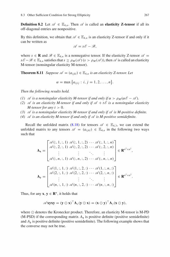
8.3 Other Sufficient Condition for Strong Ellipticity 267
Definition 8.2 Let A ∈ E4,n . Then A is called an elasticity Z-tensor if all itsoff-diagonal entries are nonpositive.
By this definition, we obtain that A ∈ E4,n is an elasticity Z-tensor if and only if itcan be written as
A = sE − B,
where s ∈ R and B ∈ E4,n is a nonnegative tensor. If the elasticity Z-tensor A =sE −B ∈ E4,n satisfies that s ≥ ρM(A ) (s > ρM(A )), then A is called an elasticityM-tensor (nonsingular elasticity M-tensor).
Theorem 8.11 Suppose A = (ai jkl) ∈ E4,n is an elasticity Z-tensor. Let
α = max{ai ji j : i, j = 1, 2, . . . , n
}.
Then the following results hold.
(1) A is a nonsingular elasticity M-tensor if and only if α > ρM(αE − A ).(2) A is an elasticity M-tensor if and only if A + tE is a nonsingular elasticity
M-tensor for any t > 0.(3) A is a nonsingular elasticity M-tensor if and only if A is M-positive definite.(4) A is an elasticity M-tensor if and only if A is M-positive semidefinite.
Recall the unfolded matrix (8.18) for tensors A ∈ E4,3, we can extend theunfolded matrix to any tensors A = (ai jkl) ∈ E4,n in the following two wayssuch that
Ax =
⎡
⎢⎢⎢⎣
A (:, 1, :, 1) A (:, 1, :, 2) · · · A (:, 1, :, n)
A (:, 2, :, 1) A (:, 2, :, 2) · · · A (:, 2, :, n)...
.... . .
...
A (:, n, :, 1) A (:, n, :, 2) · · · A (:, n, :, n)
⎤
⎥⎥⎥⎦ ∈ Rn2×n2,
Ay =
⎡
⎢⎢⎢⎣
A (1, :, 1, :) A (1, :, 2, :) · · · A (1, :, n, :)A (2, :, 1, :) A (2, :, 2, :) · · · A (2, :, n, :)
......
. . ....
A (n, :, 1, :) A (n, :, 2, :) · · · A (n, :, n, :)
⎤
⎥⎥⎥⎦ ∈ Rn2×n2.
Thus, for any x, y ∈ Rn , it holds that
A xyxy = (y � x)�Ax (y � x) = (x � y)�Ay(x � y),
where � denotes the Kronecker product. Therefore, an elasticity M-tensor is M-PD(M-PSD) if the corresponding matrix Ax is positive definite (positive semidefinite)and Ay is positive definite (positive semidefinite). The following example shows thatthe converse may not be true.
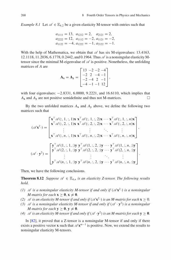
268 8 Fourth Order Tensors in Physics and Mechanics
Example 8.1 Let A ∈ E4,2 be a given elasticity M-tensor with entries such that
a1111 = 13, a1212 = 2, a2121 = 2,
a2222 = 12, a1112 = −2, a1121 = −2,
a1122 = −4, a1222 = −1, a2122 = −1.
With the help of Mathematica, we obtain that A has six M-eigenvalues: 13.4163,12.1118, 11.2036, 6.1778, 0.2442, and 0.1964. Thus A is a nonsingular elasticity M-tensor since the minimal M-eigenvalue of A is positive. Nonetheless, the unfoldingmatrices of A are
Ax = Ay =
⎡
⎢⎢⎣
13 −2 −2 −4−2 2 −4 −1−2 −4 2 −1−4 −1 −1 12
⎤
⎥⎥⎦ ,
with four eigenvalues: −2.8331, 6.0000, 9.2221, and 16.6110, which implies thatAx and Ay are not positive semidefinite and thus not M-matrices. �
By the two unfolded matrices Ax and Ay above, we define the following twomatrices such that
(A x2·) =
⎡
⎢⎢⎢⎣
x�A (:, 1, :, 1)x x�A (:, 1, :, 2)x · · · x�A (:, 1, :, n)xx�A (:, 2, :, 1)x x�A (:, 2, :, 2)x · · · x�A (:, 2, :, n)x
......
. . ....
x�A (:, n, :, 1)x x�A (:, n, :, 2)x · · · x�A (:, n, :, n)x
⎤
⎥⎥⎥⎦ ,
(A · y2) =
⎡
⎢⎢⎢⎣
y�A (1, :, 1, :)y y�A (1, :, 2, :)y · · · y�A (1, :, n, :)yy�A (2, :, 1, :)y y�A (2, :, 2, :)y · · · y�A (2, :, n, :)y
......
. . ....
y�A (n, :, 1, :)y y�A (n, :, 2, :)y · · · y�A (n, :, n, :)y
⎤
⎥⎥⎥⎦ .
Then, we have the following conclusions.
Theorem 8.12 Suppose A ∈ E4,n is an elasticity Z-tensor. The following resultshold.
(1) A is a nonsingular elasticity M-tensor if and only if (A x2·) is a nonsingularM-matrix for each x ≥ 0, x = 0.
(2) A is an elasticity M-tensor if and only if (A x2·) is an M-matrix for each x ≥ 0.(3) A is a nonsingular elasticity M-tensor if and only if (A · y2) is a nonsingular
M-matrix for each y ≥ 0, y = 0.(4) A is an elasticity M-tensor if and only if (A ·y2) is an M-matrix for each y ≥ 0.
In [82], it proved that a Z-tensor is a nonsingular M-tensor if and only if thereexists a positive vector x such that A xm−1 is positive. Now, we extend the results tononsingular elasticity M-tensors.

8.3 Other Sufficient Condition for Strong Ellipticity 269
Theorem 8.13 Suppose A ∈ E4,n is an elasticity Z-tensor. The following conditionsare equivalent:
(1) A is a nonsingular elasticity M-tensor;(2) For each x ≥ 0, x = 0, there exists y > 0 such that A xyx· > 0;(3) For each x ≥ 0, x = 0, there exists y ≥ 0, y = 0, such that A xyx· > 0;(4) For each y ≥ 0, y = 0, there exists x > 0 such that A · yxy > 0;(5) For each y ≥ 0, y = 0, there exists x ≥ 0, x = 0, such that A · yxy > 0.
By a direct computation, the condition (2) in Theorem 8.13 implies that (A x2·)y =A xyx· > 0. Let y = (y1, y2, . . . , yn)
� > 0 and D = diag(y1, . . . , yn) ∈ Rn×n .Denote A := (A x2·)D. If A is an elasticity Z-tensor, we know that A is also aZ-matrix, and
|aii | −∑
j =i
|ai j | = ai i +∑
j =i
ai j = (A xyx·)i > 0, for i ∈ [n].
Therefore A is a strictly diagonally dominant matrix. Based on this, we have thefollowing result.
Corollary 8.2 Suppose A ∈ E4,n is an elasticity Z-tensor. The following conditionshold.
(1) A is a nonsingular elasticity M-tensor if and only if or each x ≥ 0, x = 0, thereexists a positive diagonal matrix D such that D(A x2·)D is strictly diagonallydominant;
(2) A is a nonsingular elasticity M-tensor if and only if for each y ≥ 0, y = 0, thereexists a positive diagonal matrix D such that D(A · y2)D is strictly diagonallydominant.
8.4 Computational Methods for M-Eigenvalues
From the previous discussion, we know that the M-eigenvalue plays an importantrole in checking the strong ellipticity of tensors arising in nonlinear elastic materials.Hence, any numerical method for computing the minimum M-eigenvalue of a givenelasticity tensor is very applicable in the study of nonlinear elasticity and materials.In this section, we will study a practical algorithm for computing the largest M-eigenvalue of fourth order tensors, which can also be used to compute the smallestM-eigenvalue of the proposed tensors. Hence it can be used to check whether thegiven tensor satisfies the strong ellipticity or not.
For finding the largest M-eigenvalue of a tensor satisfying (8.2), we mainly aimsto consider the following optimization problem:

270 8 Fourth Order Tensors in Physics and Mechanics
max f (x, y) = ∑mi,k=1
∑nj,l=1 ai jkl xi y j xk yl
s.t. x�x = 1, y�y = 1x ∈ Rm, y ∈ Rn .
(8.25)
And the main frame of the algorithm is as follows.
Algorithm 8.2 Initialization Step. Take initial points x0 ∈ Rm , y0 ∈ Rn , and letk = 0;Iterative Step. Execute the following procedure alternatively until convergence:
x(k+1) = A · y(k)x(k)y(k), x(k+1) = x(k+1)
‖x(k+1)‖;
y(k+1) = A x(k+1)y(k)x(k+1)·, y(k+1) = y(k+1)
‖y(k+1)‖;k = k + 1.
For any given fourth order tensor A = (ai jkl) satisfying (8.2), similar to discus-sions in the previous section, let B(y) ∈ Rm×m and C(x) ∈ Rn×n are two symmetricmatrices such that
(B(y))ik =n∑
j,l=1
ai jkl y j yl , (C(x)) jl =m∑
i,k=1
ai jkl xi xk .
So, based on these two matrices, the following conclusion holds.
Theorem 8.14 For any given tensor A satisfying (8.2) and x ∈ Rm, y ∈ Rn,assume that B(y) and C(x) are both positive definite. Then the generated sequence{ f (x(k), y(k)) = A x(k)y(k)x(k)y(k)} in Algorithm 8.2 is nondecreasing.
Proof By conditions that B(y) and C(x) are both positive definite, it follows that thefunction f (x, y) is strictly convex corresponding to x ∈ Rm and y ∈ Rn respectively.Hence, for any k ≥ 0, we obtain
f (x(k+1), y(k)) − f (x(k), y(k)) ≥ 〈x(k+1) − x(k),∇x f (x(k), y(k))〉. (8.26)
Since ∇x f (x(k), y(k)) = 2A · y(k)x(k)y(k), by Algorithm 8.2, one has
x(k+1) = ∇x f (x(k), y(k))
‖∇x f (x(k), y(k))‖ .
Combining this with (8.27), recalling the Cauchy–Schwartz inequality, it holds thatf (x(k+1), y(k)) ≥ f (x(k), y(k)) and the strict inequality holds when x(k+1) = x(k).
On the other hand, it is not difficult to prove that f (x(k+1), y(k+1)) ≥ f (x(k+1), y(k))
and the strict inequality holds when y(k+1) = y(k), and the desired results hold. �
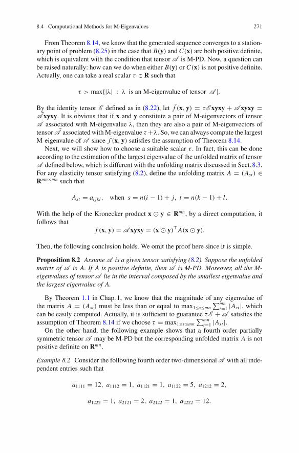
8.4 Computational Methods for M-Eigenvalues 271
From Theorem 8.14, we know that the generated sequence converges to a station-ary point of problem (8.25) in the case that B(y) and C(x) are both positive definite,which is equivalent with the condition that tensor A is M-PD. Now, a question canbe raised naturally: how can we do when either B(y) or C(x) is not positive definite.Actually, one can take a real scalar τ ∈ R such that
τ > max{|λ| : λ is an M-eigenvalue of tensor A }.
By the identity tensor E defined as in (8.22), let f (x, y) = τE xyxy + A xyxy =¯A xyxy. It is obvious that if x and y constitute a pair of M-eigenvectors of tensor
A associated with M-eigenvalue λ, then they are also a pair of M-eigenvectors oftensor ¯A associated with M-eigenvalue τ +λ. So, we can always compute the largestM-eigenvalue of A since f (x, y) satisfies the assumption of Theorem 8.14.
Next, we will show how to choose a suitable scalar τ . In fact, this can be doneaccording to the estimation of the largest eigenvalue of the unfolded matrix of tensorA defined below, which is different with the unfolding matrix discussed in Sect. 8.3.For any elasticity tensor satisfying (8.2), define the unfolding matrix A = (Ast ) ∈Rmn×mn such that
Ast = ai jkl, when s = n(i − 1) + j, t = n(k − 1) + l.
With the help of the Kronecker product x � y ∈ Rmn , by a direct computation, itfollows that
f (x, y) = A xyxy = (x � y)� A(x � y).
Then, the following conclusion holds. We omit the proof here since it is simple.
Proposition 8.2 Assume A is a given tensor satisfying (8.2). Suppose the unfoldedmatrix of A is A. If A is positive definite, then A is M-PD. Moreover, all the M-eigenvalues of tensor A lie in the interval composed by the smallest eigenvalue andthe largest eigenvalue of A.
By Theorem 1.1 in Chap. 1, we know that the magnitude of any eigenvalue ofthe matrix A = (Ast ) must be less than or equal to max1≤s≤mn
∑mnt=1 |Ast |, which
can be easily computed. Actually, it is sufficient to guarantee τE + A satisfies theassumption of Theorem 8.14 if we choose τ = max1≤s≤mn
∑mnt=1 |Ast |.
On the other hand, the following example shows that a fourth order partiallysymmetric tensor A may be M-PD but the corresponding unfolded matrix A is notpositive definite on Rmn .
Example 8.2 Consider the following fourth order two-dimensional A with all inde-pendent entries such that
a1111 = 12, a1112 = 1, a1121 = 1, a1122 = 5, a1212 = 2,
a1222 = 1, a2121 = 2, a2122 = 1, a2222 = 12.
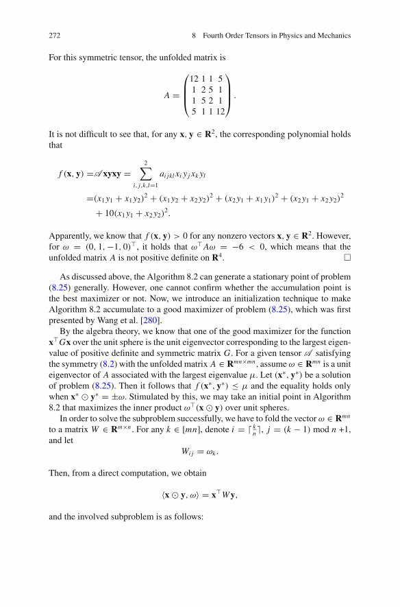
272 8 Fourth Order Tensors in Physics and Mechanics
For this symmetric tensor, the unfolded matrix is
A =
⎛
⎜⎜⎝
12 1 1 51 2 5 11 5 2 15 1 1 12
⎞
⎟⎟⎠ .
It is not difficult to see that, for any x, y ∈ R2, the corresponding polynomial holdsthat
f (x, y) =A xyxy =2∑
i, j,k,l=1
ai jkl xi y j xk yl
=(x1 y1 + x1 y2)2 + (x1 y2 + x2 y2)
2 + (x2 y1 + x1 y1)2 + (x2 y1 + x2 y2)
2
+ 10(x1 y1 + x2 y2)2.
Apparently, we know that f (x, y) > 0 for any nonzero vectors x, y ∈ R2. However,for ω = (0, 1,−1, 0)�, it holds that ω� Aω = −6 < 0, which means that theunfolded matrix A is not positive definite on R4. �
As discussed above, the Algorithm 8.2 can generate a stationary point of problem(8.25) generally. However, one cannot confirm whether the accumulation point isthe best maximizer or not. Now, we introduce an initialization technique to makeAlgorithm 8.2 accumulate to a good maximizer of problem (8.25), which was firstpresented by Wang et al. [280].
By the algebra theory, we know that one of the good maximizer for the functionx�Gx over the unit sphere is the unit eigenvector corresponding to the largest eigen-value of positive definite and symmetric matrix G. For a given tensor A satisfyingthe symmetry (8.2) with the unfolded matrix A ∈ Rmn×mn , assume ω ∈ Rmn is a uniteigenvector of A associated with the largest eigenvalue μ. Let (x∗, y∗) be a solutionof problem (8.25). Then it follows that f (x∗, y∗) ≤ μ and the equality holds onlywhen x∗ � y∗ = ±ω. Stimulated by this, we may take an initial point in Algorithm8.2 that maximizes the inner product ω�(x � y) over unit spheres.
In order to solve the subproblem successfully, we have to fold the vector ω ∈ Rmn
to a matrix W ∈ Rm×n . For any k ∈ [mn], denote i = � kn �, j = (k − 1) mod n +1,
and letWi j = ωk .
Then, from a direct computation, we obtain
〈x � y, ω〉 = x�W y,
and the involved subproblem is as follows:

8.4 Computational Methods for M-Eigenvalues 273
max x�W ys.t. x�x = 1, y�y = 1,
which is equivalent with
min ‖W − μxy�‖2F
s.t. x�x = 1, y�y = 1,
μ ∈ R.
Furthermore, the involved subproblem can be solved successfully by the singulareigenvalue decomposition of the matrix W [105], which means that if it holds that
W = U�ΣV =r∑
i=1
σi u(i)v(i)�,
where σ1 > σ2 > · · · > σr > 0, and r is the rank of the matrix, then u(1) and v(1)
constitute the solution of the subproblem. Hence, the initialization subproblem canbe solved by letting x(0) = u(1), y(0) = v(1).
By the discussion above, we have the following complete version for computingthe largest M-eigenvalue of a fourth order partially symmetric tensor.
Algorithm 8.3 Step 1: Given A = (ai jkl). Compute its unfolded matrix A = (Ai j ).1.1: Choose τ = ∑
1≤i≤ j≤mn |Ai j | and let ¯A = τE + A . Then unfold ¯A to matrix
A.1.2: Compute the eigenvector ω of matrix A associated with the largest eigenvalueand fold it into the matrix W .1.3: Compute the singular vectors u(1) and v(1) corresponding to the largest singularvalue of the matrix W .1.4: Take x0 = u(1), y0 = v(1), and let k = 0.Step 2: Execute the following procedure alternatively until certain convergence cri-terion is satisfied and output x∗, y∗:
x(k+1) = A · y(k)x(k)y(k), x(k+1) = x(k+1)
‖x(k+1)‖;
y(k+1) = A x(k+1)y(k)x(k+1)·, y(k+1) = y(k+1)
‖y(k+1)‖;k = k + 1.
Step 3: Output the largest M-eigenvalue of tensor A : λ = f (x∗, y∗) − τ , and theassociated M-eigenvectors: x∗, y∗.
For Algorithm 8.3, the computation complexity at each iterative step is of orderO(m2n + mn2). Thus the algorithm can be said to be practical if the largest M-eigenvalue of tensor A can be generated within a few steps.
274 8 Fourth Order Tensors in Physics and Mechanics
To end this section, we show that how to compute the smallest M-eigenvalue withthe proposed algorithms in this section for tensors satisfying (8.2). It is obvious thatαE − A also satisfies the partially symmetry condition (8.2) for all α ∈ R. Hence,for any given tensor A ∈ E4,n , we can always choose a sufficient large α ∈ R suchthat αE − A is M-PD, which implies that the smallest M-eigenvalue of A equalsα minus the largest M-eigenvalue of αE − A. Therefore, the algorithm proposed inthis section for computing the largest M-eigenvalue can be used to check the strongellipticity condition of a given elasticity tensor.
8.5 Higher Order Elasticity Tensors
In this section, we mainly study the M-positive definiteness (semidefiniteness) forhigher order elasticity tensors. Furthermore, for a given elasticity tensor, we con-sider the sum-of-squares (SOS) decomposition of its corresponding homogeneouspolynomials. It is obvious that an elasticity tensor is M-positive semidefinite if itscorresponding polynomial has an SOS decomposition. Moreover, necessary and suf-ficient conditions are proposed to guarantee the SOS decomposition.
The notions such that paired symmetric tensor and strongly paired symmetrictensor will be defined, and it is easy to verify that the fourth order three dimensionalelasticity tensors studied in the previous sections are all paired symmetric tensors.In addition, some higher order elasticity tensors from solid mechanics and elasticitymechanics are strongly paired symmetric tensors [123, 155, 263]. For simplicityof symbols, we only consider properties of sixth order three dimensional (strongly)paired symmetric tensors, and the obtained conclusions can be naturally extended tothe case of more higher order (strongly) paired symmetric tensors.
First of all, we introduce the definition of (strongly) paired symmetric tensor.
Definition 8.3 Let A = (ai1 j1i2 j2...im jm ) be a 2mth order n dimensional tensor. Theindices for the entries of A can be divided into m adjacent blocks {i1 j1}, . . . , {im jm}.If the entries are invariant under any permutation of indices in every block {il jl} forl ∈ [m], i.e.,
ai1 j1i2 j2...im jm = a j1i1i2 j2...im jm = ai1 j1 j2i2...im jm = · · · = ai1 j1i2 j2... jm im ,
then A is called a 2mth order n dimensional paired symmetric tensor. If the tensorfurther satisfies that the entries are invariant under any permutation of every block,then A is called a 2mth order n dimensional strongly paired symmetric tensor.
For the sake of simplicity, let P S2m,n (S P S2m,n) denote the set of all 2mth order ndimensional (strongly) paired symmetric tensors. It should be noted that, the higherorder elasticity tensors in [123, 155, 263] are strongly paired symmetric tensors andevery entry ai1 j1i2 j2...im jm is called an mth order elastic constant, which is an importantquantity in studies of elasticity theory.

8.5 Higher Order Elasticity Tensors 275
As discussed in the previous sections, we say a 2mth order n dimensional pairedsymmetric tensor A = (ai1 j1i2 j2...im jm ) is M-PSD(M-PD) if and only if
A xxyy · · · zz = A x2y2 · · · z2
=∑
i1, j1,...,im , jm∈[n]ai1 j1i2 j2...im jm xi1 x j1 yi2 y j2 · · · zim z jm ≥ (>)0,
for all (nonzero) x, y, . . . , z ∈ Rn .Particularly, a sixth order three dimensional paired symmetric tensor A satisfies
ai jklpq = a jiklpq = ai jlkpq = ai jklqp, ∀ i, j, k, l, p, q ∈ [3]. (8.27)
If A is strongly paired symmetric, it further holds that
ai jklpq = akli jpq = ai jpqkl , ∀ i, j, k, l, p, q ∈ [3]. (8.28)
The smallest M-eigenvalue for any fourth order three dimensional elasticity tensorplays an important role in verifying whether or not the proposed elasticity tensor holdsthe strong ellipticity. Similar to Definition 8.1, the definition of M-eigenvalue can beextended to the sixth order three dimensional cases. Before that, we introduce thefollowing symbols. For any paired symmetric tensor A ∈ P S6,3, let A ·xy2z2,A x2 ·yz2,A x2y2 · z ∈ R3 be defined by
(A · xy2z2)i :=3∑
j,k,l,p,q=1
ai jklpq x j yk yl z pzq , ∀ i ∈ {1, 2, 3},
(A x2 · yz2)k :=3∑
i, j,l,p,q=1
ai jklpq xi x j yl z pzq , ∀ k ∈ {1, 2, 3},
(A x2y2 · z)p :=3∑
i, j,k,l,q=1
ai jklpq xi x j yk yl zq , ∀ p ∈ {1, 2, 3}.
Then it can be verified that
〈x,A · xy2z2〉 = 〈y,A x2 · yz2〉 = 〈z,A x2y2 · z〉 = A x2y2z2.
Definition 8.4 For any paired symmetric tensor A = (ai jklpq) ∈ P S6,3, if thereexist λ ∈ R and x, y, z ∈ R3 such that
{A · xy2z2 = λx, A x2 · yz2 = λy, A x2y2 · z = λz,x�x = 1, y�y = 1, z�z = 1,
276 8 Fourth Order Tensors in Physics and Mechanics
then λ is called an M-eigenvalue of A and x, y, z are the eigenvectors of A associatedwith the M-eigenvalue λ.
From the definition, similar to Theorem 8.1, we have the following results.
Theorem 8.15 For any (strongly) paired symmetric tensor A = (ai jklpq) ∈ P S6,3,the following results hold:
(1) its M-eigenvalues always exist. Moreover, if x, y, z are the eigenvectors of Aassociated with the M-eigenvalue λ, then λ = A x2y2z2;
(2) A is M-PD if and only if its smallest M-eigenvalue is positive.
Combining Theorem 8.15 with Definition 8.4, we obtain the following result.
Theorem 8.16 For any (strongly) paired symmetric tensor A = (ai jklpq) ∈ P S6,3,
(1) λ is an M-eigenvalue of A if and only if −λ is an M-eigenvalue of −A .(2) A is positive definite if and only if the largest M-eigenvalue of −A is negative.
We say that
λ∗(x∗)2(y∗)2(z∗)2 = λ∗x∗ ⊗ x∗ ⊗ y∗ ⊗ y∗ ⊗ z∗ ⊗ z∗
is the best rank-one approximation of a given tensor A ∈ T6,3 if (λ∗, x∗, y∗, z∗) ∈R × R3 × R3 × R3 solves the optimization problem:
min ‖A − λx2y2z2‖2F
s.t. λ ∈ R and x�x = 1, y�y = 1, z�z = 1, ∀ x, y, z ∈ R3.
Based on this, we have the following conclusion for the best rank-one approximationof sixth order three dimensional paired symmetric tensors.
Theorem 8.17 For any (strongly) paired symmetric tensorA = (ai jklpq) ∈ P S6,3, ifλ∗ is an M-eigenvalue of A with the largest absolute value among all M-eigenvaluesofA , and x∗, y∗, z∗ ∈ R3 are the eigenvectors of A associated with the M-eigenvalueλ∗, then λ∗(x∗)2(y∗)2(z∗)2 is the best rank-one approximation of A .
Recall the discussion in Sect. 8.2, the M-positive definiteness of a fourth orderthree dimensional elasticity tensor can be equivalently transferred to check the posi-tive definiteness of three second order tensors, positive definiteness of a fourth ordersymmetric tensor and a sixth order symmetric tensor. Similarly, the conclusionsabove can be extended to sixth order (strongly) paired symmetric tensors. To moveon, we present three block sub-tensors for a sixth order three dimensional pairedsymmetric tensor A ∈ P S6,3. Suppose A = (ai jklpq) ∈ P S6,3, i, j, k, l, p, q ∈ [3].Denote block sub-tensors such that
Ai j := (ai jklpq )k,l,p,q∈[3], Bkl := (ai jklpq )i, j,p,q∈[3] and Cpq := (ai jklpq )i, j,k,l∈[3]. (8.29)
Then the following results are obvious.
8.5 Higher Order Elasticity Tensors 277
Proposition 8.3 For any A ∈ T6,3, let sub-tensors Ai j , Bkl and Cpq be defined by(8.29). Then it holds that
(1) if A is a paired symmetric tensor, then all sub-tensors Ai j , Bkl and Cpq arepaired symmetric tensors.
(2) if A is a strongly paired symmetric tensor, then Ast = Bst = Cst for alls, t ∈ [3].
By sub-tensors defined in (8.29), another three matrices can be defined as below
A(y, z) :=⎛
⎝A11y2z2 A12y2z2 A13y2z2
A21y2z2 A22y2z2 A23y2z2
A31y2z2 A32y2z2 A33y2z2
⎞
⎠ ,
B(x, z) :=⎛
⎝B11x2z2 B12x2z2 B13x2z2
B21x2z2 B22x2z2 B23x2z2
B31x2z2 B32x2z2 B33x2z2
⎞
⎠ ,
C(x, y) :=⎛
⎝C11x2y2 C12x2y2 C13x2y2
C21x2y2 C22x2y2 C23x2y2
C31x2y2 C32x2y2 C33x2y2
⎞
⎠ .
(8.30)
Then we know that for all x, y, z ∈ R3
A x2y2z2 = x� A(y, z)x = y� B(x, z)y = z�C(x, y)z.
Theorem 8.18 Let A ∈ P S6,3. Suppose that matrices A(y, z), B(x, z) and C(x, y)
are defined by (8.30). Then the following conditions are equivalent:
(1) The tensor A is M-PD;(2) The matrix A(y, z) is PD for all y, z ∈ R3\{0};(3) The matrix B(x, z) is PD for all x, z ∈ R3\{0};(4) The matrix C(x, y) is PD for all x, y ∈ R3\{0}.
Furthermore, if A is a strongly paired symmetric tensor, then the above (2), (3)and (4) are equivalent.
By Sylvester’s criterion that a matrix is positive definite if and only if all its leadingprincipal submatrices are positive definite, we have the following results.
Theorem 8.19 Let A ∈ P S6,3, and A(y, z), B(x, z) and C(x, y) are defined by(8.30). Then, tensor A is M-PD if and only if one of the following results holds.
(1) A11y2z2 > 0, (A11y2z2)(A22y2z2) − (A12y2z2)(A21y2z2) > 0 and det(A(y, z)) > 0 for all y, z ∈ R3\{0}.
(2) B11x2z2 > 0, (B11x2z2)(B22x2z2) − (B12x2z2)(B21x2z2) > 0 and det(B(x, z)) > 0 for all x, z ∈ R3\{0}.
(3) C11x2y2 > 0, (C11x2y2)(C22x2y2) − (C12x2y2)(C21x2y2) > 0 and det(C(x, y)) > 0 for all x, y ∈ R3\{0}.

278 8 Fourth Order Tensors in Physics and Mechanics
Furthermore, if A ∈ P S6,3 is a strongly paired symmetric tensor, then the above(1), (2) and (3) are the same.
Recall the M-positive definiteness of fourth order three dimensional elasticitytensors in Sect. 8.2, we know that it can be checked equivalently by the positivesemidefiniteness of three second order symmetric tensors, a fourth order symmetrictensor and a sixth order symmetric tensor. While an even order symmetric tensoris positive definite if and only if its smallest Z-eigenvalue is positive. Therefore,with the help of algorithm proposed by Cui, Dai and Nie [66], we can check theM-positive semidefiniteness of a fourth order elasticity tensor by computing thesmallest Z-eigenvalues of the corresponding symmetric tensors. Unfortunately, theleading principal sub-matrices of A(y, z) or B(x, z) or C(x, y) do not correspondto any symmetric tensors. Hence, we can not check the M-positive definiteness of asixth order strongly paired symmetric tensor by computing Z-eigenvalues of somesymmetric tensors.
To give the next result, the following definition is needed.
Definition 8.5 Let A = (ai1i2...i2m ) ∈ T2m,3 be a given tensor. Suppose t ∈ [1, 2m]is an even number. Then A is called a bi-block symmetric tensor if its indices{i1, i2, . . . , i2m} can be divided into two adjacent blocks
{i1, i2, . . . , it } and {it+1, it+2, . . . , i2m}
such that the entries of A being invariant under any permutation of indices in everyblock of {i1, i2, . . . , it } and {it+1, it+2, . . . , i2m}, i.e.,
ai1i2...it it+1it+2...i2m = aσ(i1i2...it )σ (it+1it+2...i2m) (8.31)
for all i1, i2, . . . , i2m ∈ {1, 2, 3}, where σ(i1i2 . . . it ) denotes an arbitrary permutationof i1i2 . . . it .
To extend the definition of M-eigenvalue to bi-block symmetric tensors, the fol-lowing symbols are needed. Suppose A ∈ T2m,3 and t ∈ [1, 2m]. Then we denote
A xt y2m−t :=3∑
i1,...,it ,it+1,...,i2m=1
ai1...it it+1...i2m xi1 . . . xt yt+1 . . . y2m;
A xt−1y2m−t ∈ R3 with entries such that
(A xt−1y2m−t )i :=3∑
i2,...,it ,it+1,...,i2m=1
aii2...it it+1...i2m xi2 . . . xt yt+1 . . . y2m, ∀ i ∈ [3];
A xt y2m−t−1 ∈ R3 with entries such that
(A xt y2m−t−1)i :=3∑
i1,...,it ,it+2,...,i2m=1
ai1...it i it+2...i2m xi1 . . . xt yt+2 . . . y2m, ∀ i ∈ [3].

8.5 Higher Order Elasticity Tensors 279
Definition 8.6 Let A = (ai1...it it+1...i2m ) ∈ T2m,3 with entries satisfying bi-blocksymmetry given by (8.31). Assume t = m, and if there exist λ ∈ R and x, y ∈ R3
such that {A xm−1ym = λx, A xmym−1 = λy,
x�x = 1, y�y = 1,
then λ is called an M-eigenvalue of A and x, y are called eigenvectors associatedwith the M-eigenvalue λ.
Similar to Theorems 8.15–8.17, we obtain the following conclusions for the bi-blocksymmetric tensors.
Theorem 8.20 Let A = (ai1...it it+1...i2m ) ∈ T2m,3 with entries satisfying bi-blocksymmetry given by (8.31). Assume t = m, then the following results hold.
(1) The M-eigenvalues of A always exist. Moreover, if x, y ∈ R3 are the eigenvectorsof A associated with the M-eigenvalue λ, then λ = A xmym.
(2) The tensor A is M-positive definite if and only if the smallest M-eigenvalue ofA is positive.
(3) λ is an M-eigenvalue of A if and only if −λ is an M-eigenvalue of −A . Further-more, A is M-positive definite if and only if the largest M-eigenvalue of −A isnegative.
(4) If λ∗ is an M-eigenvalues of A with the largest absolute value among all M-eigenvalues of A , and x∗, y∗ ∈ R3 are the eigenvectors of A associated withthe M-eigenvalue λ∗, then λ∗(x∗)m(y∗)m is the best rank-one approximation ofA .
From Theorem 8.19, one can define bi-block symmetric tensors T 1A ,T 1
B ,T 1C ∈
T8,3 and T 2A ,T 2
B ,T 2C ∈ T12,3 such that
T 1A y4z4 = (A11y2z2)(A22y2z2) − (A12y2z2)(A21y2z2), T 2
A y6z6 = det(A(y, z));
T 1B x4z4 = (B11x2z2)(B22x2z2)−(B12x2z2)(B21x2z2), T 2
B x6z6 = det(B(x, z));
T 1C x4y4 = (C11x2y2)(C22x2y2) − (C12x2y2)(C21x2y2), T 2
C x6y6 = det(C(x, y)).
Combining this with Definition 8.6, we obtain the following results.
Theorem 8.21 Let A ∈ T6,3 be a paired symmetric tensor. Then A is M-positivedefinite if and only if one of the following results holds.
(1) The smallest M-eigenvalues of tensors A11, T 1A and T 2
A are positive.(2) The smallest M-eigenvalues of tensors B11, T 1
B and T 2B are positive.
(3) The smallest M-eigenvalue of tensors C11, T 1C and T 2
C are positive.
Furthermore, if A is a strongly paired symmetric tensor, then the above (1), (2)and (3) are the same.

280 8 Fourth Order Tensors in Physics and Mechanics
In the following, we will study the sum-of-squares (SOS) decomposition for thehomogeneous polynomial corresponding to the paired symmetric tensors. In thiscase, we say that the related paired symmetric tensor is SOS if the correspondingpolynomial has an SOS decomposition. It is clear that a paired symmetric tensor isM-PSD if it is SOS. Particularly, we study the case m = 4 and m = 6, and obtainthe conclusions for any even number m > 6.
The unfolded matrix for a paired symmetric tensor is defined as below.
Definition 8.7 Suppose A = (ai jkl) ∈ T4,3 and B = (bi jklpq) ∈ T6,3 are two giventensors.(1) Define a matrix by
M = (mst ) with mst = ais it js jt ∀ s, t ∈ [9], (8.32)
where i1i2 . . . i9 and j1 j2 . . . j9 are two arbitrary permutations of 123123123 whichsatisfy that, for any r ∈ {1, 2, 3}, at least one of i3(r−1)+1i3(r−1)+2i3(r−1)+3 andj3(r−1)+1 j3(r−1)+2 j3(r−1)+3 is an arbitrary permutation of 123.(2) Define a matrix by
N = (nst ) with nst = bis it js jt ks kt ∀ s, t ∈ [27], (8.33)
where i1i2 . . . i27, j1 j2 . . . j27 and k1k2 . . . k27 are three arbitrary permutations of123123 · 123︸ ︷︷ ︸
27
which satisfy that, for any r ∈ {1, 2, . . . , 9}, at least one of
i3(r−1)+1i3(r−1)+2i3(r−1)+3, j3(r−1)+1 j3(r−1)+2 j3(r−1)+3 and k3(r−1)+1k3(r−1)+2k3(r−1)+3
is an arbitrary permutation of 123.Then we say that the matrices M is an unfolded matrix of tensor A with respect
to indices i1i2 . . . i9 and j1 j2 . . . j9 ; N is an unfolded matrix of tensor B with respectto indices i1i2 . . . i27, j1 j2 . . . j27 and k1k2 . . . k27
It should be noted that, in the previous sections, the unfolded matrices for an fourthorder elasticity tensor are concrete cases of this definition. For example, supposeA ∈ P S4,3, and M1 and M2 are defined by
M1 =⎡
⎣A11 A12 A13
A21 A22 A23
A31 A32 A33
⎤
⎦ and M2 =⎡
⎣B11 B12 B13
B21 B22 B23
B31 B32 B33
⎤
⎦ , (8.34)
where Ai j are block sub-matrices tensor A for any i, j, k, l ∈ [3] such that
Ai j := (ai jkl)kl and Bkl := (ai jkl)i j .
We can easily get that M1 is an unfolded matrix of A with respect to indices111222333 and 123123123, and M2 is an unfolded matrix with respect to indices123123123 and 111222333. In addition, we have that M1 and M2 are symmet-ric matrices, and they further satisfy that M1 = M2 when A is a strongly pairedsymmetric tensor.

8.5 Higher Order Elasticity Tensors 281
By Definition 8.7, we first give several sufficient conditions or checkable necessaryconditions for the SOS decomposition of fourth order three dimensional symmetrictensors.
Theorem 8.22 Suppose i1i2 . . . i9 and j1 j2 . . . j9 are two arbitrary permutations of123123123. Let A = (ai jkl) ∈ P S4,3 be a paired symmetric tensor. Assume M isan unfolded matrix of A with respect to indices i1i2 . . . i9 and j1 j2 . . . j9. Then, thefollowing results hold.
(1) If M is positive semidefinite, then the polynomial A x2y2 is an SOS of bilinearforms.
(2) If M is positive definite, then the tensor A is M-positive definite.(3) If A x2y2 is an SOS of bilinear forms, then it holds that aiikk ≥ 0, ∀ i, k ∈ [3].
To investigate the necessary and sufficient conditions for the SOS decompositionof tensor A ∈ P S4,3, we define tensor B ∈ T4,3 with entries such that
bi jkl = b jilk, bi jlk = b jikl , and bi jkl + b jilk + bi jlk + b jikl = 4ai jkl . (8.35)
Here, we call that B is a semi-paired symmetric tensor of A . Therefore, it followsthat A x2y2 = Bx2y2, and the conclusion below holds.
Theorem 8.23 Let A ∈ P S4,3. Suppose B is defined by (8.35) is a semi-pairedsymmetric tensor of A . Then, it holds that
(1) A x2y2 is an SOS of bilinear forms if and only if the quadratic form Bx2y2 isan SOS of bilinear forms;
(2) tensor A is M-PD (M-PSD) if and only if the tensor B is M-PD (M-PSD).
The following lemma is useful in the following discussion.
Lemma 8.2 Let A = (ai jkl) ∈ P S4,3. Assume M = (mst ) ∈ R9×9 is a symmetricmatrix such that
A x2y2 =3∑
i, j,k,l=1
ai jkl xi x j yk yl = u�Mu, ∀ x, y ∈ R3,
where the vector u = (x1 y1, x1 y2, x1 y3, x2 y1, x2 y2, x2 y3, x3 y1, x3 y2, x3 y3)�. Then
the matrix M is an unfolded matrix of some semi-paired symmetric tensor of A .
According to Lemma 8.2 and the notion of semi-paired symmetric tensor, wenow give a necessary and sufficient condition for the bilinear SOS decomposition ofthe polynomial corresponding to a fourth order three dimensional paired symmetrictensor.
Theorem 8.24 Let A = (ai jkl) ∈ P S4,3. Then A x2y2 is an SOS of bilinear formsif and only if an unfolding matrix of some semi-paired symmetric tensor of A ispositive semidefinite.
282 8 Fourth Order Tensors in Physics and Mechanics
Now, we consider the SOS decomposition for the homogeneous polynomialdefined by a sixth order three dimensional paired symmetric tensor. Similar to The-orem 8.22, the following results holds.
Theorem 8.25 Let A = (ai jklpq) ∈ P S6,3. Suppose that N defined by Definition8.7 is an unfold matrix of A with respect to indices i1i2 . . . i27, j1 j2 . . . j27 andk1k2 . . . k27. Then, we have the following conclusions.
(1) If N is positive semidefinite, then A x2y2z2 is an SOS of trilinear forms.(2) If N is positive definite, then the tensor A is M-positive definite.(3) If A x2y2z2 is an SOS of trilinear forms, then aiikkpp ≥ 0, ∀ i, k, p ∈ [3].
Similar to (8.35), we can define the semi-paired symmetric tensor for a sixth orderthree dimensional paired symmetric tensor. Suppose A = (ai jklpq) ∈ P S6,3. Definetensor B = (bi jklpq) ∈ T6,3 with entries satisfying
bi jklpq = b jilkqp, b jiklpq = bi jlkqp, bi jlkpq = b jiklqp, bi jklqp = b jilkpq , (8.36)
andbi jklpq + b jiklpq + bi jlkpq + bi jklqp = 4ai jklpq . (8.37)
We say that B is a semi-paired symmetric tensor of A .Similar to Theorems 8.23 and 8.24, we have the following results.
Theorem 8.26 Let A = (ai jklpq) ∈ P S6,3. Suppose that B is defined by (8.36) and(8.37) is an semi-paired symmetric tensor of A . Then, we have the following results.
(1) The polynomial A x2y2z2 is an SOS of trilinear forms if and only if Bx2y2z2 isan SOS of trilinear forms.
(2) Tensor A is M-positive definite (M-positive semidefinite) if and only if tensor Bis M-PD (M-PSD).
(3) A x2y2z2 an SOS of trilinear forms if and only if an unfolded matrix of somesemi-paired symmetric tensor of A is positive semidefinite.
To end this section, we note that a sequential semidefinite programming methodis established for computing the smallest M-eigenvalue of any fourth order threedimensional paired symmetric tensor [138]. Generally speaking, for a given tensorA ∈ T4,3, a new polynomial Fr,s : R3 × R3 → R is defined by
Fr,s(x, y) :=(
3∑
i=1
x2i
)r ( 3∑
i=1
y2i
)s
A x2y2,
which is a homogeneous polynomial with deg(Fr ) = 2(r + s) + 4. If A is M-PD,it is proved that Fr,s(x, y) is an SOS for some sufficiently large integers r, s ≥ 0.Denote
K := {A ∈ T4,3 : Fr,s(x, y) is an SOS for some r, s ≥ 0}.
8.5 Higher Order Elasticity Tensors 283
For any paired symmetric tensor A ∈ P S4,3, its smallest M-eigenvalue can becomputed by the optimization problem
min A x2y2
s.t. x�x = 1, y�y = 1,
which can be written equivalently as
max γ
s.t. A x2y2 ≥ γ, ∀ (x, y) ∈ {(x, y) ∈ R3 × R3 : x�x = 1, y�y = 1}. (8.38)
Suppose E = (ei jkl) ∈ T4,3 is defined by
ei jkl :={
1 if i = j, k = l,0 otherwise,
∀i, j, k, l ∈ [3].
Combining this with the set K, the optimization problem (8.38) is equivalent to
max γ
s.t. A + γE ∈ K,
which can also be relaxed to another form by the polynomial relaxation technique (fordetails see [138]). However, the method in [138] can only obtain an approximationoptimal solution up to a priori precision, and we do not know if it is efficient forcomputing the smallest M-eigenvalues of higher order paired symmetric tensors.
8.6 Notes
The strong ellipticity condition is a very important property for elasticity tensors,which have been frequently used in mechanics, including piezooptical tensor, thesecond order electrooptical effect, electrostriction and second order magnetostriction.Therefore, to verify whether or not the strong ellipticity condition holds for a givenelastic material is essential in the theory of elasticity. Actually, a lot of researchersin the field of elasticity have paid much attention to this problem [59, 106, 112,158, 159, 236, 244, 271, 276]. To be different with the previous methods, in thischapter, we mainly study the strong ellipticity of elasticity tensors by spectral theoryof tensors.
Section 8.1: The definition of M-eigenvalues for elasticity tensors was first definedby Qi, Dai and Han in [226]. It is also proved that the fourth order three dimensionalelasticity tensor satisfies strong ellipticity condition if and only if its smallest M-eigenvalue is positive. The main sufficient condition for M-positive definiteness isthe S-positive definiteness. The S-positive definiteness of elasticity tensors has beenstudied by Lord Kelvin in [261, 262] 160 years ago. In the special case such that

284 8 Fourth Order Tensors in Physics and Mechanics
m = n = 2, a direct method was proposed to compute the smallest M-eigenvalue.Details about resultant of a system for two variables can be obtained in [102].
Section 8.2: For the strong ellipticity condition of fourth order three dimensionalelasticity tensors, an efficient sufficient and necessary condition was proposed viaZ-eigenvalues of symmetric tensors by Han, Dai and Qi [114]. The notion of Z-eigenvalue of symmetric tensors was first defined by Qi in [221]. More results aboutZ-eigenvalues for symmetric tensors can be found in [228]. A special kinds of ellip-ticity tensor for the rhombic system has been studied in [59]. Here, we present ansufficient and necessary condition for the rhombic system via a symmetric copositivematrix. The concrete sufficient and necessary conditions for a 3×3 symmetric matrixto be copositive was given by Simpson and Spector [244].
Section 8.3: The content of this section was originally given by Ding, Qi and Yan[85] and Ding, Liu, Qi and Yan [79]. The related M-tensors were first studied byDing, Qi and Wei [82] and Zhang, Qi and Zhou [305]. More results about M-tensorcan be found in the book [228].
Section 8.4: The practical algorithm studied in this section was given by Wang,Qi and Zhang in [280]. The power method was first used to compute the largestH-eigenvalue by Ng, Qi and Zhou in 2009 [197].
Section 8.5: The study in this section was originally given by Huang and Qi in2017 [138]. Some concrete models for higher order elasticity tensors from solidmechanics and elasticity mechanics can be found in Hiki [123], Jong et al. [155],and Thurston and Brugger [263].
8.7 Exercises
1 Suppose A = (ai jkl) ∈ E4,3 be given by
a1111 = 1, a2222 = 1, a3333 = 1, a1122 = 2, a2233 = 2, a3311 = 2,
a1212 = a1221 = a2112 = a2121 = − 12 , a2323 = a2332 = a3223 = a3232 = − 1
2 ,
a3131 = a3113 = a1331 = a1313 = − 12 .
Please prove that the given tensor is M-positive definite.2 Suppose that λ = 0 is an M-eigenvalue of the elasticity tensor A in last question.By the definition of M-eigenvalue for elasticity tensors, write the M-eigenvectorscorresponding to the M-eigenvalue λ = 0.3 Suppose A ∈ E4,3 is an elasticity M-tensor. Prove that A is a nonsingular elasticityM-tensor if and only if the unfolded matrix (A · y2) is a nonsingular M-matrix foreach y ≥ 0.4 Suppose A ∈ E4,3 is an elasticity tensor such that
a1111 = a1122 = a1133 = a2211 = a2222 = a2233 = a3311 = 1,
a3322 = 3, a3333 = 3, a3323 = a3332 = −1, other ai jkl = 0.
Prove that λ = 1 is the smallest M-eigenvalue for tensor A . Furthermore, give theM-eigenvectors corresponding to λ = 1.
Chapter 9Higher Order Tensors in QuantumPhysics
In this chapter, we will apply tensor analysis to the quantum entanglement problemand the classicality problem of spin states in quantum physics.
The quantum entanglement problem is one of the most important problems inquantum physics and quantum information technology. The central question is: giv-ing a quantum state, can one determine whether it is entangled or not? In the literature,several approaches to measure entanglement of a state are proposed, e.g., hyperde-terminant, tensor rank, etc. Among others, geometric measure is a newly proposedmeasure for quantum entanglement. In this chapter, we will study the geometric mea-sure of a quantum state by using spectral theory of tensors. It will establish a bridgebetween the recently developed spectral theory of tensors and a central problem inquantum physics.
Mathematically, a general n-partite state of a composite quantum system canbe regarded as an element in a Hilbert tensor product space. Generally speaking,a separable state can be viewed as a rank-one tensor in this tensor space, and thegeometric measure is a measure of the distance between a given state and the set ofseparable states. This distance can be characterized by taking the maximization of ahomogeneous form over the set of separable states, which is called Hartree value.
We will show how the spectral theory of non-negative tensors can be applied to thestudy of the geometric measure of entanglement for pure states. For symmetric puremultipartite qubit or qutrit states, an elimination method is given. For symmetric puremultipartite qudit states, a numerical algorithm with randomization is presented. Wewill also illustrate that a nonsymmetric pure state can be augmented to a symmetricone whose amplitudes can be encoded in a non-negative symmetric tensor, and thenthe geometric measure of entanglement can be calculated. Several examples, such asmGHZ states, W states, inverted W states, qudits, and nonsymmetric states, are usedto demonstrate the power of the proposed methods. Given a pure state, one may finda change of basis (a unitary transformation) so that all the probability amplitudes ofthe pure state are non-negative under the new basis. Therefore, the methods proposedhere can be applied to a very wide class of multipartite pure states.
© Springer Nature Singapore Pte Ltd. 2018L. Qi et al., Tensor Eigenvalues and Their Applications, Advances in Mechanicsand Mathematics 39, https://doi.org/10.1007/978-981-10-8058-6_9
285

286 9 Higher Order Tensors in Quantum Physics
Furthermore, we will study the connection between the smallest Z-eigenvalue ofa tensor and the entanglement of a pure or mixed state. This originates in the fact thatthe entanglement of a state is related to the positive semi-definiteness of a tensor,which in turn is linked to the sign of its smallest Z-eigenvalue.
We will define the unitary eigenvalue (U-eigenvalue) of a complex tensor, the uni-tary symmetric eigenvalue (US-eigenvalue) of a symmetric complex tensor, and thebest complex rank-one approximation. An upper bound on the number of distinct US-eigenvalues of symmetric tensors will be given, and we will count all US-eigenpairswith nonzero eigenvalues of symmetric tensors. We will convert the geometric mea-sure of the entanglement problem to an algebraic equation system problem. A numer-ical example shows that a symmetric real tensor may have a best complex rank-oneapproximation that is better than its best real rank-one approximation, which impliesthat the absolute-value of the largest Z-eigenvalue is not always the geometric mea-sure of entanglement.
We will then consider mixed states. The geometric measure of quantum entangle-ment of a pure state, defined by its distance to the set of pure separable states, can beextended to multipartite mixed states. We will characterize the nearest disentangledmixed state to a given mixed state with respect to the geometric measure by meansof a system of equations. The entanglement eigenvalue of a mixed state will be intro-duced. And we will show that, for a given mixed state, its nearest disentangled mixedstate is associated with its entanglement eigenvalue.
A geometrical picture of quantum states often helps us get some insight on under-lying physical properties. For arbitrary pure spin states, such a geometrical repre-sentation was developed by Ettore Majorana [192]: a spin- j state is visualized asN = 2 j points on the unit sphere S2, called in this context the Bloch sphere. Theadvantage of such a picture is a direct interpretation of certain unitary operations:namely, if a quantum spin- j state is mapped to another one by a unitary operationthat corresponds to a (2 j + 1)-dimensional representation of a spatial rotation, itsMajorana points are mapped to points obtained by that spatial rotation. Recentlya tensor representation of an arbitrary mixed or pure spin- j state was proposed togeneralizes this picture [103]. It consists of a real symmetric tensor of order N = 2 jand dimension 4. A spin- j state corresponds to a boson if j is a positive integer, andcorresponds to a fermion if j is a positive half-integer. Thus, a boson corresponds toan even order four dimensional tensor, while a fermion corresponds to an odd orderfour dimensional tensor.
Recently, Qi, Zhang, Braun, Bohnet-Waldraff and Giraud [233] introducedregularly decomposable tensors and showed that a spin- j state is classical if andonly if its representing tensor is a regularly decomposable tensor. An algorithm wasproposed to determine if the representing tensor of a spin state is regularly decom-posable or not.
9.1 Quantum Entanglement Problems 287
9.1 Quantum Entanglement Problems
In 1935, Albert Einstein, Boris Podolsky and Nathan Rosen described a “spooky”phenomenon, which is known as EPR paradox. They demonstrated that in quantummechanics the knowledge of one physical quantity precluded the knowledge of theother one even when they were described by non-commuting operators, and thusbelieved “the quantum mechanical description of physical reality given by wavefunctions is not complete [90].” The word “entanglement” was first given by ErwinSchrödinger when writing a letter to Einstein to discuss the correlations between twoparticles. This problem lay dormant for many years until 1964, when John StewartBell showed that if the locality assumption held, then the completion of quantummechanics did not exist in the sense of EPR.
Bell’s work provided us the chance of regarding entanglement as a resource forapplication. Quantum entanglement is an extremely active topic in physics commu-nity. Experimental entanglement of photons, neutrinos, electrons, and even smalldiamonds is widely studied and effectively demonstrated [15, 209]. Furthermore,quantum entanglement is applied in communication and computation. The bigachievement of quantum entanglement application was made in 2016, when Chi-nese quantum satellite sent ‘spooky’ messages over 1,200 km — 12 times morethan ever before — in a move that could enable massive breakthroughs in securecommunications.
Next let us make the concept of quantum entanglement concrete. In quantummechanics, it means pairs or groups of particles interacted mutually and the quantumstate of each particle cannot be described independently of the others, even when thedistance between the particles is large. This physical phenomenon is called quantumentanglement. In fact, when we say entanglement, we refer to a multipartite system,whose Hilbert space can be presented as a product of two or more tensor factorsaccording to physical subsystems of this system. If a global state of a compositesystem can be expressed as a product of the states of subsystems, it is called adisentangled or separable system. Otherwise, we call this state entangled.
In this section, we mainly focus on the entanglement problem of pure states.Mathematically, a quantum state corresponds to a vector of norm 1 in a Hilbert spaceover the complex numbers, while a mixed state is a probabilistic mixture of purestates. To describe a state vector, i.e., a pure quantum state, we follows the custom inquantum mechanics by using bra–ket notation, which contains the angle brackets “〈”and “〉”, and vertical bar “|”. Each bra 〈Ψ | is the conjugate transpose of the so-calledket |Ψ 〉, which are related to the same quantum state.
Definition 9.1 Suppose that H is a Hilbert tensor product space
H = H1 ⊗ · · · ⊗ Hm,
288 9 Higher Order Tensors in Quantum Physics
and the dimension of Hk is dk for k ∈ [m]. We denote |Ψ 〉 as a general m-partitestate of a composite quantum system. Then, |Ψ 〉 may be regarded as an element ofH , i.e.,
|Ψ 〉 ∈ H and 〈Ψ |Ψ 〉 = 1,
in which 〈·|·〉 means the inner product. If an m-partite state |φ〉 ∈ H could be rep-resented as
|φ〉 = |φ(1)〉 ⊗ · · · ⊗ |φ(m)〉, (9.1)
where |φ(k)〉 ∈ Hk and ‖|φ(k)〉‖ = 1 for k ∈ [m], then |φ〉 is called a separable (i.e.,Hartree) m-partite state. The set of all separable m-partite states in H is denotedas Sep(H ). A pure state of a composite quantum system is entangled if it is notseparable.
For example, given two basis vectors {|0〉A, |1〉A} of H1 and two basis vectors{|0〉B, |1〉B} of H2, one of the famous Bell state
|Ψ 〉 = 1√2
(|0〉A ⊗ |1〉B − |1〉A ⊗ |0〉B)
is an entangled state.Measuring physical properties such as position, momentum, spin, and polariza-
tion, we find that entangled particles are appropriately correlated. For example, if thetotal spin of two entangled particles is zero, we put them in Beijing and Hongkongseparately and measure the spin of each particle on the same axis. When the spin ofthe particle in Hongkong (Beijing) is found to be clockwise (counterclockwise), thespin of the particle in Beijing (Hongkong) will be discovered as counterclockwise(clockwise). Since the outcome of the measurement is random and no one transmitinformation in the experiment, it seems that when we operate on one particle, theother one “knows” the operation and “alter” its spin according to the result of its part-ner, even when they are separated by large distance. This is also the basic quantumentanglement theory that ensure truly secure communication in the Chinese quantumsatellite.
9.2 Geometric Measure of Entanglement of MultipartitePure States
Assume that d1 ≤ · · · ≤ dm without loss of generality in Definition 9.1. The degreeof which a general m-partite state |Ψ 〉 ∈ H is entangled could be characterized bythe distance to the set Sep(H ) [243, 284]:
dist = ‖|Ψ 〉 − |φΨ 〉‖ = min{‖|Ψ 〉 − |φ〉‖ : |φ〉 ∈ Sep(H )}, (9.2)

9.2 Geometric Measure of Entanglement of Multipartite Pure States 289
where |φΨ 〉 ∈ Sep(H ) is the nearest separable m-partite state of |Ψ 〉. The distancein (9.2) stands for a natural geometric measure of the entanglement content. Thefarther a state from the set of separable m-partite states is, the more entangled it is.In addition, we remark that since the objective of (9.2) is a continuous function andthe feasible region is a compact set in a finite dimensional space, there always existsthe nearest separable m-partite state |φΨ 〉.
For a general m-partite state |Ψ 〉 and an arbitrary separable m-partite state |φ〉 =⊗k∈[m]|φ(k)〉 in (9.1), we have
‖|Ψ 〉 − |φ〉‖2 = 2 − 〈Ψ |φ〉 − 〈φ|Ψ 〉. (9.3)
To characterise the minimization problem (9.2), we study its dual maximizationproblem
max{〈Ψ |φ〉 + 〈φ|Ψ 〉 : |φ〉 ∈ Sep(H )} (9.4)
= max{〈Ψ |(⊗k∈[m]|φ(k)〉) + (⊗k∈[m]〈φ(k)|)|Ψ 〉 : 〈φ(k)|φ(k)〉 = 1 for k ∈ [m]} .
By introducing Lagrange multipliers λk for k ∈ [m], we obtain
〈Ψ |(⊗ j =k |φ( j)〉) = λk〈φ(k)| and (⊗ j =k〈φ( j)|)|Ψ 〉 = λk |φ(k)〉. (9.5)
Multiplying them by |φ(k)〉 and 〈φ(k)|, we see that
λ := λk = 〈Ψ |φ〉 = 〈φ|Ψ 〉 (9.6)
is a real number in [−1, 1].Motivated by (9.3) and (9.6), we denote
GΨ := max{|〈Ψ |φ〉| : |φ〉 ∈ Sep(H )} (9.7)
the maximal overlap of a fixed m-partite pure state |Ψ 〉 ∈ H . We see that the maximaloverlap in (9.7) is equal to the largest entanglement eigenvalue λ satisfying thefollowing polynomial system
⎧⎨
⎩
〈Ψ |(⊗ j =k |φ( j)〉) = λ〈φ(k)|,(⊗ j =k〈φ( j)|)|Ψ 〉 = λ|φ(k)〉,
‖|φ(k)〉‖ = 1, k ∈ [m].(9.8)
Next, we introduce the minimum Hartree value, and show that the geometry measureof the entanglement content of |Ψ 〉 is bounded up by the Hartree value [222].
Theorem 9.1 We call
σ := min{〈Ψ |φΨ 〉 : |Ψ 〉 ∈ H , 〈Ψ |Ψ 〉 = 1}
290 9 Higher Order Tensors in Quantum Physics
the minimum Hartree value of H , where |φΨ 〉 is the nearest separable m-partitestate to |Φ〉. Therefore, σ > 0, and 〈Ψ |φΨ 〉 ≥ σ for any |Ψ 〉 ∈ H . Furthermore,the geometry measure of the entanglement content of |Ψ 〉 satisfies
dist = ‖|Ψ 〉 − |φΨ 〉‖ ≤ √2 − 2σ . (9.9)
Proof For the function
g(|z〉) := max{|〈z|φ〉| : |φ〉 ∈ Sep(H )}, where |z〉 ∈ H ,
we see that g(|z〉) ≥ 0 and g(|z〉) = 0 if and only if |z〉 = 0. Moreover, for |z〉, |w〉 ∈H , we have g(|z〉 + |w〉) ≤ g(|z〉) + g(|w〉). Hence, g(·) defines a norm in the finitedimensional space H . Recalling another norm h(|z〉) = √〈z|z〉 defined also in H ,and according to the norm equivalence theorem in the finite dimensional space, weget
σ = min{〈Ψ |φΨ 〉 : |Ψ 〉 ∈ H , 〈Ψ |Ψ 〉 = 1}≥ min{g(|Ψ 〉) : |Ψ 〉 ∈ H , h(|Ψ 〉) = 1}> 0.
Hence 〈Ψ |φΨ 〉 ≥ σ > 0 for any |Ψ 〉 ∈ H .Now, for the dual problem (9.4), we have
max{〈Ψ |φ〉 + 〈φ|Ψ 〉 : |φ〉 ∈ Sep(H )} = 〈Ψ |φΨ 〉 + 〈φΨ |Ψ 〉 ≥ 2σ.
Hence, the inequality (9.9) for the primal problem is valid. �
The following theorem reveals a lower bound for the minimum Hartree value[222].
Theorem 9.2 A lower bound for the minimum Hartree value σ of H is
σ ≥ 1√d1 · · · dm−1
. (9.10)
Proof In general, we suppose that |e(k)ik
〉 for ik ∈ [dk] is an orthonormal basis of Hk
for k ∈ [m]. Under these bases, we could write
|Ψ 〉 =∑
i1,...,im
ai1...im |e(1)i1
〉 · · · |e(m)im
〉 and |φ(k)〉 =∑
ik∈[dk ]u(k)
ik|e(k)
ik〉.

9.2 Geometric Measure of Entanglement of Multipartite Pure States 291
Let A = (ai1...im ) be a supermatrix and u(k) = (u(k)ik
) for k ∈ [m]. We define
ρ(A ) := max
⎧⎨
⎩
∣∣∣∣∣∣
∑
i1,...,im
ai1...im u(1)i1
· · · u(m)im
∣∣∣∣∣∣: ‖u(k)‖ = 1 for k ∈ [m]
⎫⎬
⎭. (9.11)
In fact, we say ρ(A ) = 〈Ψ |φΨ 〉 = max{|〈Ψ |φ〉| : φ = ⊗k∈[m]|φ(k)〉 ∈ Sep(H )}.Now, we consider slice matrices Ai1...im−2 of which the (i, j)th element is ai1...im−2i j
for i ∈ [dm−1] and j ∈ [dm]. By (9.11), we see
ρ(Ai1...im−2) ≤ ρ(A ), ∀ i1, . . . , im−2.
We say that ρ(Ai1...im−2) is the spectral norm of a matrix Ai1...im−2 and
‖Ai1...im−2‖F ≤ √dm−1ρ(Ai1...im−2) ∀ i1, . . . , im−2.
Because of 〈Ψ |Ψ 〉 = 1, we have ‖A ‖F = 1. Combining these inequalities, we get
1 = ‖A ‖2F
=∑
i1,...,im−2
‖Ai1...im−2‖2F
≤∑
i1,...,im−2
dm−1ρ(Ai1...im−2)2
≤∑
i1,...,im−2
dm−1ρ(A )2
= d1 · · · dm−1ρ(A )2.
Hence, for any Ψ ∈ H with 〈Ψ |Ψ 〉 = 1, we have
〈Ψ |φΨ 〉 = ρ(A ) ≥ 1√d1 · · · dm−1
.
Because σ = min{〈Ψ |φΨ 〉 : Ψ ∈ H , 〈Ψ |Ψ 〉 = 1}, we obtain the lower bound(9.10). �
We note that when m = 2, the minimum Hartree value is σ = 1√d1
. The lower
bound is attainable. Let A be a diagonal tensor with diagonal elements aii = 1√d1
for i ∈ [d1]. Then we see that |Ψ 〉 is a pure state. By setting φΨ = |e(1)1 〉 ⊗ |e(2)
1 〉, weobtain σ = 〈Ψ |φΨ 〉 = 1√
d1straightforwardly.
292 9 Higher Order Tensors in Quantum Physics
Using these two theorems, we say that the geometric measure of the entanglementcontent of |Ψ 〉 ∈ H is bounded above
dist = ‖|Ψ 〉 − |φΨ 〉‖ ≤ √2 − 2σ ≤
√
2 − 2√d1 · · · dm−1
.
9.3 Z-Eigenvalues and Entanglement of Symmetric States
We consider a special Hilbert tensor product space H ⊗m and the dimension of His n. Let |Ψ 〉 ∈ H ⊗m be an m-partite symmetric pure state with 〈Ψ |Ψ 〉 = 1. An m-partite symmetric pure separate state could be represented as |φ〉⊗m , where |φ〉 ∈ Hand 〈φ|φ〉 = 1. By (9.8), the quantum eigenvalue problem could be rewritten as
⎧⎨
⎩
〈Ψ |(|φ〉⊗m−1) = λ〈φ|,(〈φ|⊗m−1)|Ψ 〉 = λ|φ〉,
〈φ|φ〉 = 1.
(9.12)
By choosing an orthonormal basis of H , the symmetric pure state |Ψ 〉 is rep-resented by an mth order n dimensional symmetric complex tensor AΨ . The state|φ〉 is represented by an n dimensional complex vector z. The equality 〈φ|φ〉 = 1reduces to zH z = 1, where (·)H means the conjugate transpose of complex vectors.Then, the quantum eigenvalue problem (9.12) could be formulated as [309]
⎧⎨
⎩
AΨ zm−1 = λz,AΨ zm−1 = λz,
zH z = 1.
(9.13)
Obviously, if there exist λ ∈ C and z ∈ C satisfying (9.13), then λ is real. We call λ
a quantum eigenvalue of the tensor AΨ and z the associated quantum eigenvector.The largest quantum eigenvalue of AΨ is named as the entanglement eigenvalue ofAΨ , which is associated with the nearest separable state of the state Ψ .
Since λ is real, the system (9.13) is equivalent to
⎧⎨
⎩
AΨ zm−1 = λz,zH z = 1,
λ ∈ R.
(9.14)
Next, we show that quantum eigenvalues appear in pairs [309].
Proposition 9.1 If λ ∈ R is a quantum eigenvalue of a symmetric tensor AΨ , then−λ is a quantum eigenvalue of AΨ , too.
9.3 Z-Eigenvalues and Entanglement of Symmetric States 293
Proof Suppose that λ is a quantum eigenvalue of AΨ and z is the associated quantumeigenvector. By direct calculations, −λ is also a quantum eigenvalue of AΨ with anassociated quantum eigenvector z exp( π
m i), where i is the imaginary unit. �
The above property means that the quantum spectral radius of AΨ is the largestquantum eigenvalue of AΨ . For convenience, we denote Q(Ψ ) as the quantum spec-tral radius of AΨ and Z(Ψ ) as the largest quantum eigenvalue of AΨ . Then we havethe following theorem [132, 309].
Theorem 9.3 If the symmetric tensor AΨ of an m-partite pure state |Ψ 〉 is real, then
Q(Ψ ) ≥ Z(Ψ ).
In addition, the equality holds in the following five cases:
(1) m = 2;(2) AΨ is diagonal;(3) AΨ is nonnegative;(4) AΨ is nonpositive;(5) AΨ =∑ j∈[n] α j (y( j))m, where α j , j ∈ [n], are real numbers, {y( j)} j∈[n] is an
orthonormal basis of Rn.
Proof According to definitions of quantum eigenvalues and Z-eigenvalues of a realtensor AΨ , a Z-eigenvalue λ of AΨ is also a quantum eigenvalue. In addition, byProposition 9.1, |λ| is a quantum eigenvalue of AΨ . Hence, we have Q(Ψ ) ≥ Z(Ψ ).
To prove the equivalence of Q(Ψ ) and Z(Ψ ), we only need to prove Q(Ψ ) ≤Z(Ψ ).
(1) Let λ be an entanglement eigenvalue of AΨ and z = x + iy be the associatedentanglement eigenvector, where x, y are real vectors and one of them are nonzeroat least. Hence, we have AΨ x = λx and AΨ y = −λy. If x is nonzero, (λ, x
‖x‖ ) isa Z-eigenpair of AΨ . If y is nonzero, (−λ,
y‖y‖ ) is a Z-eigenpair of AΨ . Recalling
Proposition 9.1, we claim that Q(Ψ ) ≤ Z(Ψ ).(2) We consider a real diagonal tensor AΨ = diag(a1, . . . , an). Denote |ai | =
max{|ak | : k ∈ [n]}. Obviously, ai is a Z-eigenvalue of AΨ with its associated Z-eigenvector ei . This means that Z(Ψ ) ≥ |ai |.
Suppose that (λ, z) is an entanglement eigenpair of AΨ . Since z = 0, there existsa component z j = 0. From zH z = 1, we know |z j | ≤ 1. By a j z
m−1j = λz j , we have
Q(Ψ ) = λ ≤ |a j ||z j |m−2 ≤ |ai | ≤ Z(Ψ ).
(3) By the spectral theory of nonnegative tensors, the Z-spectral radius Z(Ψ ) is aZ-eigenvalue of the nonnegative tensor AΨ and
Z(Ψ ) = maxx∈Rn+∩Sn−1
AΨ xm = maxx∈Sn−1
AΨ xm = Q(Ψ ),
where Sn−1 = {x ∈ Rn : x x = 1}.

294 9 Higher Order Tensors in Quantum Physics
(4) Since −AΨ is nonnegative, we have Z(Ψ ) = Z(−Ψ ) = Q(−Ψ ) = Q(Ψ ) bythe above assertion.
(5) Suppose that λ is an entanglement eigenvalue of AΨ with the associatedeigenvector z. Then, we have
∑
j∈[n]α j
(y( j) z
)m−1y( j) = λz. (9.15)
Since {y( j)} is an orthonormal basis of Rn , there exists an index k such that y(k) z = 0.By multiplying y(k) on both sides of (9.15), we get
λy(k) z =∑
j∈[n]α j
(y( j) z
)m−1 (y(k) y( j)
)
= αk
(y(k) z
)m−1.
Hence, we get
Q(Ψ ) = λ ≤ |αk |∣∣∣y(k) z
∣∣∣m−2 ≤ |αk |.
Let x = y(k) ∈ Rn . Then, x x = 1 and AΨ xm−1 = αkx. Thus, αk is a Z-eigenvalueof AΨ and hence Z(Φ) ≥ |αk | ≥ Q(Ψ ). The proof is complete. �
Generally speaking, the inequality Q(Ψ ) = Z(Ψ ) holds. In [140], a counterexample is given and verifies this conclusion.
If Q(Ψ ) = Z(Ψ ) holds, the problem of finding the entanglement eigenvalue ofan m-partite pure state Ψ could be transformed into the problem of finding the Z-spectral radius of AΨ . Whereafter, we show some examples [132]. For 0 ≤ k ≤ m,we define
|S(m, k)〉 :=√
k!(m − k)!m!
∑
τ∈Gm
∣∣∣∣∣∣τ(0 . . . 0︸ ︷︷ ︸
k
1 . . . 1︸ ︷︷ ︸m−k
)
⟩
,
where Gm is the symmetric group on m elements.Example 1. The mGHZ state is of the form
|mGHZ〉 = |S(m, 0)〉 + |S(m, m)〉√2
.
Under the basis {|0〉, |1〉}, we get AmG H Z ∈ Sm,2. By calculations, its Z-eigenpairsare

9.3 Z-Eigenvalues and Entanglement of Symmetric States 295
(1√2, (1, 0)
),
(1√2, (0, 1)
),
(1√
2m−1 ,
(1√2, 1√
2
) ),
and five more when m is odd(
1√2, (−1, 0)
),
(1√2, (0,−1)
),
(1√
2m−1 ,
(− 1√
2, 1√
2
) ),
(1√
2m−1 ,
(1√2,− 1√
2
) ),
(1√
2m−1 ,
(− 1√
2,− 1√
2
) ).
Hence, we obtain Q(mG H Z) = Z(mG H Z) = 1√2. The corresponding nearest sep-
arable pure state is |φ〉⊗m where |φ〉 = |0〉 or |φ〉 = |1〉.Example 2. For a three-partite qubit, the W state is of the form
|W 〉 = |S(3, 2)〉 = |001〉 + |010〉 + |100〉√3
.
Under the basis {|0〉, |1〉}, we get AW ∈ S3,2. By calculations, its Z-eigenpairs are
(0, (0, 1) ),(23 ,(√
23 ,
√13
) ),
(23 ,(−√
23 ,
√13
) ),
(− 2
3 ,(√
23 ,−
√13
) ),
(− 2
3 ,(−√
23 ,−
√13
) ).
Hence, Q(W ) = Z(W ) = 23 . The corresponding nearest separable pure state is |φ〉⊗3
with |φ〉 =√
23 |0〉 +
√13 |1〉.
296 9 Higher Order Tensors in Quantum Physics
Example 3. For a three-partite qubit, the inverted-W state is of the form
|W 〉 = |S(3, 1)〉 = |110〉 + |101〉 + |011〉√3
.
Under the basis {|0〉, |1〉}, we get AW ∈ S3,2. By switching components of Z-eigenvectors, the Z-eigenpairs for AW become that for AW . Hence, Q(W ) =Z(W ) = 2
3 and the corresponding nearest separable pure state is |φ〉⊗3 with |φ〉 =√13 |0〉 +
√23 |1〉.
Example 4. For a three-partite qutrit, the general GHZ state is of the form
|Ψ 〉 = α|111〉 + β|222〉 + γ |333〉, α2 + β2 + γ 2 = 1.
Under the basis {|1〉, |2〉, |3〉}, we get AΨ ∈ S3,3 and it is nonnegative when α, β, γ ≥0. By calculations, its nonnegative Z-eigenpairs are
(α, (1, 0, 0) ),
(β, (0, 1, 0) ),
(γ, (0, 0, 1) ),(αβ√α2+β2
,
(β√
α2+β2, α√
α2+β2, 0
) )
,
(αγ√α2+γ 2
,
(γ√
α2+γ 2, 0, α√
α2+γ 2
) )
,
(βγ√β2+γ 2
,
(0,
γ√β2+γ 2
,β√
β2+γ 2
) )
,
(αβγ
τ,(
βγ
τ,
αγ
τ,
αβ
τ
) ),
where τ := √α2β2 + β2γ 2 + α2γ 2.Hence, Q(W ) = Z(W ) = max{α, β, γ } when α, β, γ ≥ 0. The corresponding
nearest separable pure state is |φ〉⊗3 with |φ〉 = |1〉 when Q(W ) = α, |2〉 whenQ(W ) = β, or |3〉 when Q(W ) = γ .
Example 5. Given a multipartite qudit state |Φ〉 as follows
|Φ〉 = 1
2
4∑
i=1
|i〉 ⊗ · · · ⊗ |i〉︸ ︷︷ ︸4
.
By the algorithm proposed in [66], we get Q(Φ) = Z(Φ) = 0.5 and the associatedZ-eigenvectors are (1, 0, 0, 0) , (0, 1, 0, 0) , (0, 0, 1, 0) , and (0, 0, 0, 1) .

9.4 Geometric Measure and U-Eigenvalues of Tensors 297
9.4 Geometric Measure and U-Eigenvalues of Tensors
LetA ∈ Cn1×···×nm be an mth order complex tensor and x(i) ∈ Cni be complex vectorsfor i ∈ [m]. Then ⊗i∈[m]x(i) forms an mth order complex tensor with rank-one. Wedefine
〈A ,⊗i∈[m]x(i)〉 =∑
i1,...,im
Ai1...im x (1)i1
· · · x (m)im
.
Moreover, we define vectors 〈A ,⊗i =kx(i)〉 and 〈⊗i =kx(i),A 〉, whose componentsare
〈A ,⊗i =kx(i)〉ik :=∑
i1,...,ik−1,ik+1,...,im
Ai1...ik ...im x (1)i1
· · · x (k−1)ik−1
x (k+1)ik+1
· · · x (m)im
,
〈⊗i =kx(i),A 〉ik :=∑
i1,...,ik−1,ik+1,...,im
Ai1...ik ...im x (1)i1
· · · x (k−1)ik−1
x (k+1)ik+1
· · · x (m)im
.
A complex number λ is called a unitary eigenvalue of a tensor A ∈ Cn1×···×nm
[199] if there exist complex vectors x(k) ∈ Cnk satisfying the following system
⎧⎨
⎩
〈A ,⊗i =kx(i)〉 = λx(k),
〈⊗i =kx(i),A 〉 = λx(k), ∀k ∈ [m].‖x(k)‖ = 1,
(9.16)
In fact, the largest |λ| is the entanglement eigenvalue of A , and the correspondingrank-one tensor ⊗i∈[m]x(i) is the nearest separable state.
More specifically, for the symmetric case, we assume that S ∈ Cn×···×n is asymmetric tensor. For x ∈ Cn , we denote
S xm := 〈S ,⊗i∈[m]x〉 =∑
i1,...,im
Si1...im xi1 · · · xim ,
and a vector S xm−1 whose components are
(S xm−1) j :=∑
i2,...,im
S j i2...im xi2 · · · xim .
A complex number λ is called a unitary symmetric eigenvalue of S [199], if thereexists a vector x ∈ Cn satisfying
⎧⎨
⎩
S xm−1 = λx,
S xm−1 = λx,
‖x‖ = 1.
(9.17)
298 9 Higher Order Tensors in Quantum Physics
The complex vector x is named a unitary symmetric eigenvector of S associatedwith the unitary symmetric eigenvalue λ, and (λ, x) is called a unitary symmetriceigenpair. The largest |λ| is the entanglement eigenvalue of S , and the correspond-ing rank-one tensor ⊗i∈[m]x is the nearest symmetric separable state.
Theorem 9.4 Suppose that tensors S ∈ Cn1×···×nm . Then,(a) all unitary eigenvalues of S are real;(b) if S is a complex symmetric tensor, its unitary symmetric eigenpair (λ, x) couldalso be defined as ⎧
⎨
⎩
S xm−1 = λx,
‖x‖ = 1,
λ ∈ R.
(9.18)
or ⎧⎨
⎩
S xm−1 = λx,
‖x‖ = 1,
λ ∈ R.
(9.19)
Proof (a) Suppose that λ is a unitary eigenvalue of A with an associated rank-onetensor ⊗i∈[m]x(i). By multiplying x(k) and x(k) to the first and second equations of(9.16), we have
〈A ,⊗i∈[m]x(i)〉 = λ = 〈⊗i∈[m]x(i),A 〉.
From the definition of inner product of complex tensors, we have
〈A ,⊗i∈[m]x(i)〉 = 〈⊗i∈[m]x(i),A 〉.
Hence, the unitary eigenvalue λ is a real number.(b) Since λ is real, the second equation in (9.17) is the conjugate of the first
equation in (9.17). Hence, (9.18) and (9.19) are equivalent to (9.17). �
For a complex symmetric tensor S , if (λ, x) is its unitary symmetric eigenpair,then (λ, x) is its quantum eigenpair. Note that ⊗i∈[m]x, but not ⊗i∈[m]x, is relatedto the nearest separable state. This is the main advantage of the unitary eigenpair ofcomplex tensors.
Theorem 9.5 Suppose that S is a complex symmetric tensor of order m.(a) If m ≥ 3 is an odd integer and λ = 0, then the system (9.17) is equivalent to
S xm−1 = x, x = 0.
(b) If m ≥ 3 is an even integer and λ = 0, then the system (9.17) is equivalent to
S xm−1 = ±x, x = 0.
9.4 Geometric Measure and U-Eigenvalues of Tensors 299
Proof (a) Suppose that (λ, x) is a unitary symmetric eigenpair of S . Then, λ isreal. If λ = 0, we define μ := λ−1/(m−2) which is also real because m ≥ 3 is odd. Bysetting y = μx, (9.18) equals
S ym−1 = y.
On the other hand, if there exists a nonzero complex vector y satisfying the aboveequation, the pair (λ, x) with
λ = ±‖y‖−(m−2) and x = y‖y‖ .
is a unitary eigenpair of S .(b) It can be proved by a similar approach for part (a). �
Theorem 9.6 Suppose that S is a symmetric complex tensor and λ is its unitarysymmetric eigenvalue. Then(a) −λ is also a unitary symmetric eigenvalue of S ;(b) Q(S) = λmax, where λmax is the largest unitary symmetric eigenvalue of S .
Proof (a) By (9.18), if (λ, x) is a unitary symmetric eigenpair of S , (−λ, exp( πm i)x)
is also a unitary symmetric eigenpair of S .(b) The assertion is straightforward by (a). �
Next, we turn to the best symmetric complex rank-one approximation of symmet-ric tensors, i.e., the closest symmetric product state problems. Let S be a complexsymmetric tensor. We try to find a unit vector x∗ such that
S (x∗)m = max{|S xm | : xH x = 1}. (9.20)
Then, we have the following theorem [199].
Theorem 9.7 The best symmetric complex rank-one approximation problem (9.20)is equivalent to the following optimization problem
min{‖x‖ : S xm−1 = x, 0 = x ∈ Cn}.
Proof It is clear that S (x∗)m = λmax is the largest unitary symmetric eigenvalueof S . Then, this theorem follows from Theorems 9.5 and 9.4. �
9.5 Regularly Decomposable Tensors and Classical SpinStates
In quantum theory and many related areas such as solid-state physics, molecular,atomic, high-energy physics, the concept of spin is widely used. With the recentadvance of quantum information theory, the classicality of spin states becomes more
300 9 Higher Order Tensors in Quantum Physics
and more important and has gained much attention. In literature, researchers proposedseveral different definitions of classicality of a quantum state, such as the one basedupon the positivity of the Wigner function, or the absence of entanglement in multi-partite systems. Analogous to the classicality of the harmonic oscillator states ofthe electromagnetic field, the classicality of a spin state is well-defined in terms ofits density matrix which can be decomposed as a positive weighted sum of angularmomentum coherent states. Recently, a compact and elegant representation of spindensity matrices in terms of 4-dimensional tensors that share the most importantproperties of Bloch vectors was introduced. Especially, the classicality property ofa spin state, either a boson or a fermion, can be fully characterized by the regulardecomposability of the corresponding representing tensor [233]. In this regard, theidentification of the classicality of a spin state can be fully accomplished by theverification of the regular decomposability of the corresponding tensor.
Suppose A ∈ Sm,n+1 is a real symmetric tensor. We call A a completely decom-posable tensor if there exist vectors u(1), . . . , u(r) ∈ Rn+1 such that
A =∑
i∈[r ](u(i))⊗m, (9.21)
where (u(i))⊗m = u(i) ⊗ · · · ⊗ u(i) is a rank-one tensor.
Definition 9.2 A vector x = (x0, x1, . . . , xn) ∈ Rn+1 is called a regular vector if
x0 = 0 and x20 = x2
1 + · · · + x2n .
Definition 9.3 Let A = (ai1i2...im ) ∈ Sm,n+1. We define its j th row tensor A j =(a j,i2...im ) as a symmetric tensor in Sm−1,n+1 for j ∈ [n].Definition 9.4 (a) Let m = 2 be an even integer and A ∈ Sm,n+1. We say thatA ∈ R2 ,n+1 is a regularly decomposable tensor of even order if A is completelydecomposable as (9.21) and u(1), . . . , u(r) ∈ Rn+1 therein are regular vectors.
(b) Let m = 2 + 1 be an odd integer and A ∈ Sm,n+1. If its row tensor A0 is aregularly decomposable tensor with the regularly decomposition
A0 =∑
k∈[r ](u(k))⊗2 ,
where u(k) = (u(k)0 , . . . , u(k)
n ) for k ∈ [r ] are regular vectors, and the other rowtensors of A are induced by the following formula
A j =∑
k∈[r ]
u(k)j
u(k)0
(u(k))⊗2 ,
for j ∈ [n], we call A a regularly decomposable tensor of odd order.
The regular decomposability of a symmetric tensor was originally definedseparately in even order case and in odd order case via special rank-one tensor

9.5 Regularly Decomposable Tensors and Classical Spin States 301
decompositions. However, a unified characterization for both even and odd ordertensors was further established.
Theorem 9.8 A tensor A = (ai1...im ) ∈ Sm,n+1 is a regularly decomposable tensor
if and only if there exist an integer r , some αk > 0 and v(k) =(
1, v(k)1 , . . . , v(k)
n
)
satisfying∑
i∈[n]
(v(k)
i
)2 = 1 for k ∈ [r ] such that
A =∑
k∈[r ]αk(v(k))⊗m
. (9.22)
Proof Suppose that m = 2 is even, A is defined by (9.21), and u(1), . . . , u(r) areregular vectors. By setting
v(k) = u(k)
u(k)0
and
αk =(
u(k)0
)2
> 0
for k ∈ [r ], we obtain the expression (9.22). On the other hand, A can be written
as (9.22). Since α12
k v(k) are regular vectors, A is a regularly decomposable tensor.Thus, this theorem is valid in the even order case.
The odd case can be proved similarly. �
If a tensor A = (ai1...im ) ∈ Sm,n+1 satisfies
a00i3...im =∑
i∈[n]aiii3...im ,
then A is called a regular symmetric tensor. Then, we have the following criticaltheorem [233].
Theorem 9.9 A spin- j state can be represented by a regular symmetric tensor A ∈S2 j,4. A spin- j state is classical if and only if its representing tensor A is a regularlydecomposable tensor.
By this theorem, the physical problem to determine whether a spin- j state isclassical or not is converted to a mathematical problem of identifying the regulardecomposability of its representing tensor.
We call R a normalized orthogonal matrix if
R =(
1 0 0 Q
),
where Q is an orthogonal matrix and 0 ∈ Rn is a zero vector.

302 9 Higher Order Tensors in Quantum Physics
Theorem 9.10 Suppose that A ,B ∈ Sm,n+1, R is a normalized orthogonal matrix,and B = RmA . Then, B is regularly decomposable if and only if A is regularlydecomposable.
Proof Suppose that A is regularly decomposable. From Theorem 9.8, there existpositive numbers αk and regular vectors v(k) = (1, v(k)
) with v(k) ∈ Rn being unit
vectors for k ∈ [r ] satisfying (9.22). Then
B = RmA =∑
k∈[r ]αk(Rv(k)
)⊗m.
Clearly, since R is a normalized orthogonal matrix, we have
Rv(k) =(
1 0 0 Q
)(1
v(k)
)=(
1Qv(k)
)
and Qv(k) are also unit vectors for k ∈ [r ]. Hence, Rv(k) are regular vectors fork ∈ [r ] and B is a regularly decomposable tensor.
The other part can be proved similarly by using the normalized orthogonal matrixR−1. �
For notational convenience, we use RDm,n+1 to denote the set of all regularlydecomposable tensors in Sm,n+1.
Theorem 9.11 RDm,n+1 is a closed convex cone.
Proof By Theorem 9.8, it is easy to see that RDm,n+1 is a convex cone. Next, weprove its closeness.
Let {A (p)}p=1,2,... be a convergent sequence of regularly decomposable tensorsin RDm,n+1, and
limp→∞ A (p) = A .
According to Theorem 9.8, we assume that
A (p) =∑
k∈[rp]αk,p
(v(k,p)
)⊗m,
whereαk,p ≥ 0, v(k,p) = (1, v(k,p)) with‖v(k,p)‖ = 1 for k ∈ [rp] and p = 1, 2, . . . .By the Carathéodory theory, we have
rp ≤(
m + n + 2
m
)+ 1.

9.5 Regularly Decomposable Tensors and Classical Spin States 303
Hence, without loss of generality, there is a common r = rp ≤ (m+n+2m
)+ 1 for allp. By taking a subsequence if necessary, there exist αk ≥ 0, regular vectors v(k) =(1, v(k)) such that
limp→∞ αk,p = αk,
limp→∞ v(k,p) = v(k),
andA =
∑
k∈[r ]αk(v(k))⊗m ∈ RDm,n+1.
Hence, RDm,n+1 is closed. �
However, to verify the membership of a tensor A ∈ RDm,n+1 is generally NP-hard.
It is known that the classicality of a spin- j state is equivalent to the regulardecomposibility of its representing tensor A ∈ S2 j,4. Together with the equivalentcharacterization of regularly decomposable tensors in Theorem 9.8, we will dis-cuss an E-truncated K-moment problem model for the identification of the desiredclassicality in this section.
Before transforming the characterization to an E-truncated K-moment problem,some necessary preliminaries on polynomials are briefly recalled. We use R[x] :=R[x1, . . . , xn] to denote the ring of all polynomials in x := (x1, . . . , xn)
∈ Rn withreal coefficients, and R[x]d the space of all polynomials in R[x] whose degreesare at most d. Apparently, the dimension of R[x]d is
(n+dd
). An ideal of R[x] is
a subset J of R[x] such that J · R[x] ⊆ J and J + J ⊆ J . Let h := (h1, . . . , hr )
with each hi in R[x]. The ideal generated by h, termed as I (h), is exactly the setr∑
i=1hi R[x]. The kth truncated ideal generated by h, denoted by Ik(h), is defined
as the setr∑
i=1hi R[x]k−deg(hi ), where deg(hi ) denotes the degree of the polynomial
hi . Obviously, ∪k∈N Ik(h) = I (h), where N is the set of all nonnegative integers. Apolynomial p ∈ R[x] is called a sum of squares (SOS) if there exist q1, . . . , qm ∈R[x] such that p =
m∑
i=1q2
i . We use �[x] to denote the set of all SOS polynomials
and �[x]k to denote the intersection of �[x] and R[x]k . The set Qk(h) := �[x]2k +r∑
i=1hi�[x]2k−deg(hi ) is called the kth quadratic module generated by h and the union
Q(h) := ∪k≥0 Qk(h) is called the quadratic module generated by h.For any vector x = (x1, . . . , xn)
and any α := (α1, . . . , αn), denote xα :=xα1
1 · · · xαnn and |α| :=
n∑
i=1αi . Denote Nn
d := {α ∈ Nn : |α| ≤ d}, e.g., N22 = {(0, 0),
(0, 1), (1, 0), (2, 0), (1, 1), (0, 2)}. Let RNnd be the real sequences indexed by α ∈ Nn
d ,
304 9 Higher Order Tensors in Quantum Physics
i.e., RNnd := {y : y = (yα)α∈Nn
d}, e.g., y = (y00, y01, y10, y20, y11, y02)
∈ RN22 . Each
y ∈ RNnd is called a truncated moment sequence (tms) of degree d.
Let E := {α ∈ Nn+1 : |α| = m}. Then, each index (i1, . . . , im) corresponds to avector
∑
j∈[m]1(i j ) ∈ E , where each 1(i j ) ∈ Rn+1 is the i j th unit vector. In this regard,
each symmetric tensor corresponds to a unique identifying vector
a = (aα)α∈E ∈ RE := {a : a = (aα)α∈E , aα ∈ R}.
The vector a is called an E-truncated moment sequence (E-tms for short) of A .Let
K := {x ∈ Rn+1 : x x − 2 = 0, x1 − 1 = 0}. (9.23)
Obviously, K is a compact set in Rn+1. By employing Theorem 9.8, a tensor A ∈RDm,n+1 if and only if there exist αk > 0 and v(k) =
(1, v(k)
1 , . . . , v(k)n
) ∈ K for
k = 1, . . . , r such that
A =r∑
k=1
αk(v(k))⊗m
. (9.24)
For any given a ∈ RE , a nonnegative Borel measure μ supported in K is called aK -representing measure for a if
aα =∫
Kxαdμ, ∀α ∈ E .
Recall that a measure is called finitely atomic if its support is a finite set, and is calleda r-atomic if its support consists of at most r distinct points (more details see [202]).Therefore,
A ∈ RDm,n+1 ⇐⇒ (9.25)
the identifying vector a of A admits a K -representing measure,
where K is defined in (9.23).Denote R[x]E := span{xα : α ∈ E}. Obviously, R[x]E is a linear subspace of
R[x]m . For a polynomial p ∈ R[x]E , p|K ≥ 0(> 0) denotes that p(x) ≥ 0(> 0)
for any x ∈ K . Recall from [96] that R[x]E is K -full if there exists a polynomialp ∈ R[x]E such that p|K > 0. By choosing p(x) := xm
1 > 0 in our case, it is easilyseen that R[x]E is K -full.
Given a tms y, we define the Riesz functional Ly acting on R[x]d in the mannerthat
Ly(p(x)) = Ly(∑
α∈N nd
pαxα) :=∑
α∈N nd
pα yα,
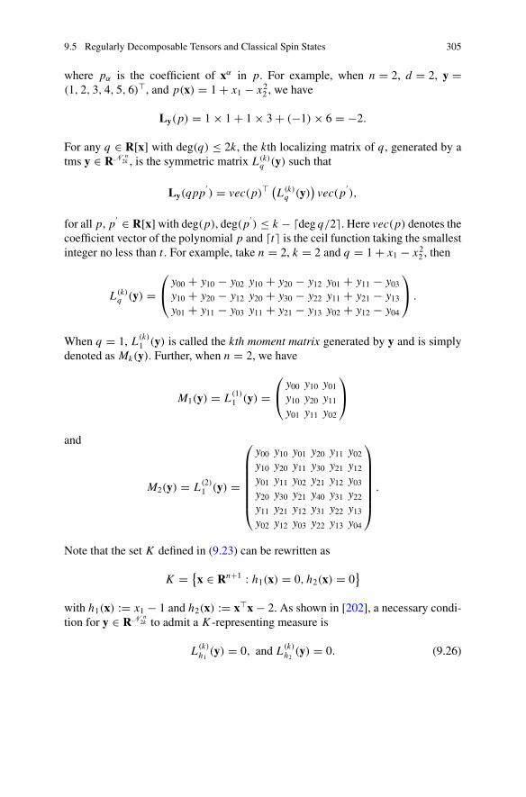
9.5 Regularly Decomposable Tensors and Classical Spin States 305
where pα is the coefficient of xα in p. For example, when n = 2, d = 2, y =(1, 2, 3, 4, 5, 6) , and p(x) = 1 + x1 − x2
2 , we have
Ly(p) = 1 × 1 + 1 × 3 + (−1) × 6 = −2.
For any q ∈ R[x] with deg(q) ≤ 2k, the kth localizing matrix of q, generated by atms y ∈ RN n
2k , is the symmetric matrix L(k)q (y) such that
Ly(qpp′) = vec(p)
(L(k)
q (y))
vec(p′),
for all p, p′ ∈ R[x] with deg(p), deg(p
′) ≤ k − �deg q/2�. Here vec(p) denotes the
coefficient vector of the polynomial p and �t� is the ceil function taking the smallestinteger no less than t . For example, take n = 2, k = 2 and q = 1 + x1 − x2
2 , then
L(k)q (y) =
⎛
⎝y00 + y10 − y02 y10 + y20 − y12 y01 + y11 − y03
y10 + y20 − y12 y20 + y30 − y22 y11 + y21 − y13
y01 + y11 − y03 y11 + y21 − y13 y02 + y12 − y04
⎞
⎠ .
When q = 1, L(k)1 (y) is called the kth moment matrix generated by y and is simply
denoted as Mk(y). Further, when n = 2, we have
M1(y) = L(1)1 (y) =
⎛
⎝y00 y10 y01
y10 y20 y11
y01 y11 y02
⎞
⎠
and
M2(y) = L(2)1 (y) =
⎛
⎜⎜⎜⎜⎜⎜⎝
y00 y10 y01 y20 y11 y02
y10 y20 y11 y30 y21 y12
y01 y11 y02 y21 y12 y03
y20 y30 y21 y40 y31 y22
y11 y21 y12 y31 y22 y13
y02 y12 y03 y22 y13 y04
⎞
⎟⎟⎟⎟⎟⎟⎠
.
Note that the set K defined in (9.23) can be rewritten as
K = {x ∈ Rn+1 : h1(x) = 0, h2(x) = 0}
with h1(x) := x1 − 1 and h2(x) := x x − 2. As shown in [202], a necessary condi-tion for y ∈ RN n
2k to admit a K -representing measure is
L(k)h1
(y) = 0, and L(k)h2
(y) = 0. (9.26)
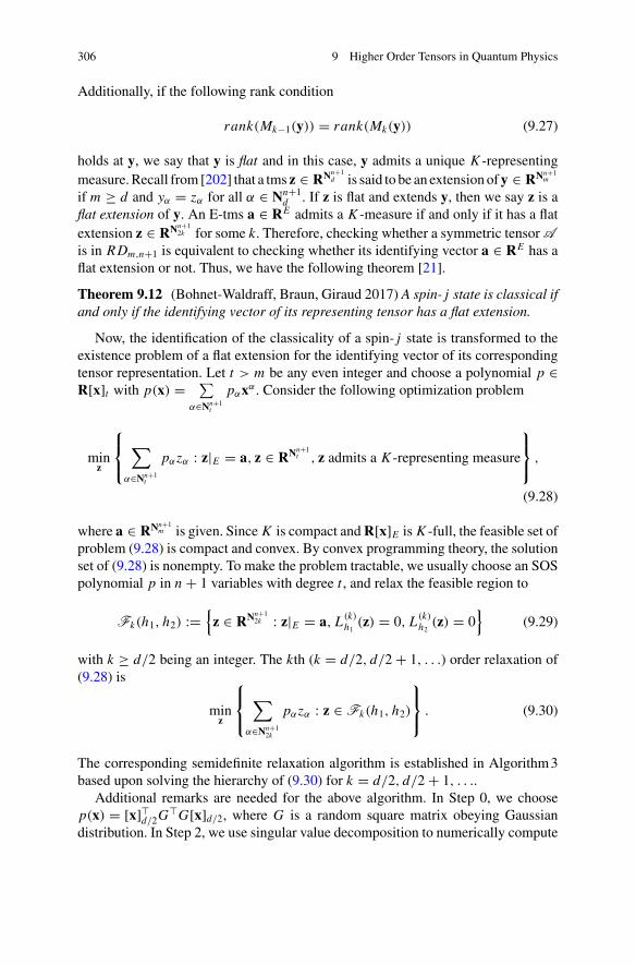
306 9 Higher Order Tensors in Quantum Physics
Additionally, if the following rank condition
rank(Mk−1(y)) = rank(Mk(y)) (9.27)
holds at y, we say that y is flat and in this case, y admits a unique K -representingmeasure. Recall from [202] that a tms z ∈ RNn+1
d is said to be an extension of y ∈ RNn+1m
if m ≥ d and yα = zα for all α ∈ Nn+1d . If z is flat and extends y, then we say z is a
flat extension of y. An E-tms a ∈ RE admits a K -measure if and only if it has a flatextension z ∈ RNn+1
2k for some k. Therefore, checking whether a symmetric tensor Ais in RDm,n+1 is equivalent to checking whether its identifying vector a ∈ RE has aflat extension or not. Thus, we have the following theorem [21].
Theorem 9.12 (Bohnet-Waldraff, Braun, Giraud 2017) A spin- j state is classical ifand only if the identifying vector of its representing tensor has a flat extension.
Now, the identification of the classicality of a spin- j state is transformed to theexistence problem of a flat extension for the identifying vector of its correspondingtensor representation. Let t > m be any even integer and choose a polynomial p ∈R[x]t with p(x) = ∑
α∈Nn+1t
pαxα . Consider the following optimization problem
minz
⎧⎨
⎩
∑
α∈Nn+1t
pαzα : z|E = a, z ∈ RNn+1t , z admits a K -representing measure
⎫⎬
⎭,
(9.28)
where a ∈ RNn+1m is given. Since K is compact and R[x]E is K -full, the feasible set of
problem (9.28) is compact and convex. By convex programming theory, the solutionset of (9.28) is nonempty. To make the problem tractable, we usually choose an SOSpolynomial p in n + 1 variables with degree t , and relax the feasible region to
Fk(h1, h2) :={
z ∈ RNn+12k : z|E = a, L(k)
h1(z) = 0, L(k)
h2(z) = 0
}(9.29)
with k ≥ d/2 being an integer. The kth (k = d/2, d/2 + 1, . . .) order relaxation of(9.28) is
minz
⎧⎨
⎩
∑
α∈Nn+12k
pαzα : z ∈ Fk(h1, h2)
⎫⎬
⎭. (9.30)
The corresponding semidefinite relaxation algorithm is established in Algorithm 3based upon solving the hierarchy of (9.30) for k = d/2, d/2 + 1, . . ..
Additional remarks are needed for the above algorithm. In Step 0, we choosep(x) = [x] d/2G G[x]d/2, where G is a random square matrix obeying Gaussiandistribution. In Step 2, we use singular value decomposition to numerically compute

9.5 Regularly Decomposable Tensors and Classical Spin States 307
Algorithm 3 A relaxation algorithm to identify the classicality of a spin- j stateInput: The tensor representation A of a spin- j state;Output: The certification of non-classicality or the coefficients αk ’s and the vectors vk ’s to generate
a decomposition of A as described in (9.22);
0 Compute the identifying vector a from A . Choose a generic SOS polynomial p and setk = d/2.
1 Solve (9.30). If (9.30) is infeasible, then output a certificate that the spin- j state is not classicaland stop. Otherwise, compute a solution z∗(k). Let l = 1.
2 compute r1 := rank(Mk−1(z∗(k)|2l) and r2 := rank(Mk(z∗(k)|2l). If r1 = r2, then go toStep 4, otherwise go to Step 3.
3 Compute the finite atomic measure μ admitted by z∗(k)|2l as follows:
μ =∑
k∈[r ]αkδ(v(k)),
where αk > 0, v(k) ∈ K , r = rank(Ml(z∗(k)|2l), and δ(v(k)) is the Dirac measure supportedon point v(k) (k = 1, . . . , r ). Stop.
4 If l < k, set l = l + 1 and go to Step 2; Otherwise, set k = k + 1 and go to Step 1.
Return: A certificate or αk , v(k) for k ∈ [r ].
the desired rank values by counting the number of the singular values greater than10−6. In Step 3, the method was proposed in [121] to get the measure μ. By invokingthat R[x]E is K -full, the following convergence results follow readily from [202].
Theorem 9.13 For Algorithm3, we have
(a) If (9.30) is infeasible for some k, then the spin- j state is not classical;(b) If the spin- j state is not classical, then (9.30) is infeasible for all k big enough;(c) If the spin- j state is classical, then for almost all generated p, we can asymp-
totically get a flat extension of a by solving the hierarchy of (9.30).
The first experiment is for the following randomly generated cases with n = 3and (m, r) in different positive integer values.
(a) Randomly generate x(k) = randn(1, n) and set v(k) =(
1, x(k)
‖x(k)‖)
for k =1, . . . , r to get the corresponding representation tensor A . (Obviously, all suchgenerated tensors are regularly decomposable tensors.) Results are listed inTable 9.1.
(b) Randomly generate symmetric tensors A ∈ Sm,n with a11i3...im =n+1∑
i=2aiii3...im + 1
for some randomly chosen index (i3, . . . , im). (It is known from Theorem 9.8 thatnone of such A ’s are regularly decomposable.) Results are listed in Table 9.2.
The second experiment is testing on the data of entangled states and classicalstates. Each class contains 100 spin- j states for different j ranging from 1 to 3. As weknow, tensors corresponding to the classical states are regularly decomposable, while
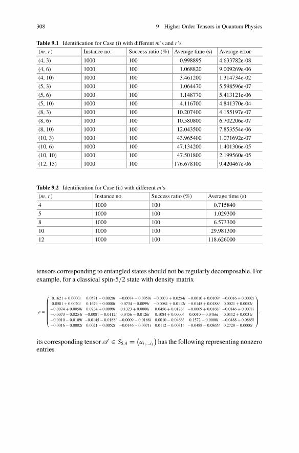
308 9 Higher Order Tensors in Quantum Physics
Table 9.1 Identification for Case (i) with different m’s and r ’s
(m, r) Instance no. Success ratio (%) Average time (s) Average error
(4, 3) 1000 100 0.998895 4.633782e-08
(4, 6) 1000 100 1.068820 9.009269e-06
(4, 10) 1000 100 3.461200 1.314734e-02
(5, 3) 1000 100 1.064470 5.598596e-07
(5, 6) 1000 100 1.148770 5.413121e-06
(5, 10) 1000 100 4.116700 4.841370e-04
(8, 3) 1000 100 10.207400 4.155197e-07
(8, 6) 1000 100 10.580800 6.702206e-07
(8, 10) 1000 100 12.043500 7.853554e-06
(10, 3) 1000 100 43.965400 1.071692e-07
(10, 6) 1000 100 47.134200 1.401306e-05
(10, 10) 1000 100 47.501800 2.199560e-05
(12, 15) 1000 100 176.678100 9.420467e-06
Table 9.2 Identification for Case (ii) with different m’s
(m, r) Instance no. Success ratio (%) Average time (s)
4 1000 100 0.715840
5 1000 100 1.029300
8 1000 100 6.573300
10 1000 100 29.981300
12 1000 100 118.626000
tensors corresponding to entangled states should not be regularly decomposable. Forexample, for a classical spin-5/2 state with density matrix
ρ =
⎛
⎜⎜⎜⎜⎜⎜⎜⎝
0.1621 + 0.0000i 0.0581 − 0.0020i −0.0074 − 0.0050i −0.0073 + 0.0254i −0.0010 + 0.0109i −0.0016 + 0.0002i0.0581 + 0.0020i 0.1679 + 0.0000i 0.0734 − 0.0099i −0.0081 + 0.0112i −0.0145 + 0.0188i 0.0021 + 0.0052i
−0.0074 + 0.0050i 0.0734 + 0.0099i 0.1323 + 0.0000i 0.0456 + 0.0126i −0.0009 + 0.0168i −0.0146 + 0.0071i−0.0073 − 0.0254i −0.0081 − 0.0112i 0.0456 − 0.0126i 0.1084 + 0.0000i 0.0010 + 0.0466i 0.0112 + 0.0031i−0.0010 − 0.0109i −0.0145 − 0.0188i −0.0009 − 0.0168i 0.0010 − 0.0466i 0.1572 + 0.0000i −0.0488 + 0.0865i−0.0016 − 0.0002i 0.0021 − 0.0052i −0.0146 − 0.0071i 0.0112 − 0.0031i −0.0488 − 0.0865i 0.2720 − 0.0000i
⎞
⎟⎟⎟⎟⎟⎟⎟⎠
,
its corresponding tensor A ∈ S5,4 = (ai1...i5
)has the following representing nonzero
entries

9.5 Regularly Decomposable Tensors and Classical Spin States 309
Table 9.3 The αk ’s andv(k)’s of the regulardecomposition of A
αk ’s (v(k)) ’s
0.1153 (1.0000 −0.6399 −0.1329 −0.7568)
0.0744 (1.0000 −0.2910 −0.3733 −0.8808)
0.0073 (1.0000 −0.5795 −0.8084 0.1027)
0.0352 (1.0000 −0.7261 0.1853 −0.6619)
0.0950 (1.0000 0.0344 −0.6409 −0.7667)
0.0424 (1.0000 0.1770 −0.9618 −0.2088)
0.0714 (1.0000 0.1108 0.0316 −0.9933)
0.0646 (1.0000 0.7443 −0.3981 −0.5361)
0.0751 (1.0000 −0.2113 −0.4739 0.8549)
0.1314 (1.0000 0.7745 −0.5572 0.2995)
0.0307 (1.0000 −0.0240 0.3697 0.9289)
0.1271 (1.0000 0.1990 0.8833 0.4246)
0.0800 (1.0000 0.7009 −0.0452 0.7118)
0.0504 (1.0000 0.7741 0.4804 0.4123)
a11111 = 1, a11112 = 0.1472, a11122 = 0.2693, a11222 = 0.0923, a12222 = 0.1354,
a22222 = 0.0588, a11113 = −0.1322, a11123 = −0.0226, a11223 = −0.0511, a12223 = −0.0303,
a22223 = −0.0280, a11133 = 0.2797, a11233 = 0.0647, a12233 = 0.0471, a22233 = 0.0273,
a11333 = −0.0106, a12333 = −0.0014, a13333 = 0.1556, a22333 = −0.0123, a23333 = 0.0324,
a33333 = 0.0121, a11114 = −0.0987, a11124 = 0.1366, a11224 = −0.0047, a12224 = 0.0661,
a22224 = 0.0034, a11134 = 0.1111, a11234 = 0.0067, a12234 = 0.0044, a22234 = −0.0019,
a11334 = 0.0229, a12334 = 0.0159, a13334 = 0.0596, a22334 = 0.0076, a23334 = 0.0082,
a33334 = 0.0198, a11144 = 0.4510, a11244 = −0.0099, a12244 = 0.0868, a22244 = 0.0062,
a11344 = −0.0705, a12344 = 0.0091, a13344 = 0.0770, a22344 = −0.0108, a23344 = 0.0051,
a33344 = −0.0104, a11444 = −0.1169, a12444 = 0.0546, a13444 = 0.0471, a14444 = 0.2872,
a22444 = −0.0157, a23444 = 0.0004, a24444 = −0.0212, a33444 = −0.0044, a34444 = −0.0493,
a44444 = −0.0968.
Using Algorithm 3, we can identify its classicality and obtain an approximate decom-
position B :=14∑
k=1αk(v(k))⊗5 with the relative error η := ‖A −B‖F
‖A ‖F= 5.495371e-05.
The αk’s and v(k)’s are listed in Table 9.3.And for an entangled spin-2 state with density matrix
ρ =
⎛
⎜⎜⎜⎜⎝
0.1852 + 0.0000i −0.0737 − 0.0362i −0.0482 + 0.0792i 0.0579 + 0.0692i 0.0812 − 0.0258i−0.0737 + 0.0362i 0.0997 + 0.0000i −0.0231 − 0.0642i −0.0860 + 0.0117i −0.0572 − 0.0316i−0.0482 − 0.0792i −0.0231 + 0.0642i 0.2556 + 0.0000i 0.0465 − 0.1158i 0.0445 − 0.0175i0.0579 − 0.0692i −0.0860 − 0.0117i 0.0465 + 0.1158i 0.1144 + 0.0000i 0.0274 + 0.0255i0.0812 + 0.0258i −0.0572 + 0.0316i 0.0445 + 0.0175i 0.0274 − 0.0255i 0.3452 + 0.0000i
⎞
⎟⎟⎟⎟⎠
,
its corresponding tensor A ∈ S4,4 = (ai1...i4
)has the following representing nonzero
entries
310 9 Higher Order Tensors in Quantum Physics
a1111 = 1, a1112 = 0.0480, a1122 = 0.1660, a1222 = −0.0292,
a2222 = 0.0536, a1113 = 0.0107, a1123 = 0.0324, a1223 = −0.0387,
a2223 = 0.0169, a1133 = 0.3337, a1233 = 0.0373, a1333 = 0.0540,
a2233 = 0.0522, a2333 = 0.0206, a3333 = 0.2100, a1114 = 0.0580,
a1124 = 0.0231, a1224 = −0.0026, a2224 = 0.0038, a1134 = −0.0604,
a1234 = −0.0032, a1334 = 0.0068, a2234 = −0.0086, a2334 = 0.0031,
a3334 = −0.0291, a1144 = 0.5003, a1244 = 0.0399, a1344 = −0.0046,
a1444 = 0.0538, a2244 = 0.0602, a2344 = −0.0051, a2444 = 0.0162,
a3344 = 0.0714, a3444 = −0.0227, a4444 = 0.3686.
Implement Algorithm 3, a certificate of non-classicality is given for such an entan-gled state.
9.6 Notes
Recently, Chinese quantum satellite, named Micius, has sent “spooky action” mes-sages over 1,200 km. This news motivates and encourages us to study in quantumphysics and related areas.
Section 9.1 The physical phenomenon of quantum entanglement studied in [20,89, 209] is different from classical physics.
Section 9.2 The conception of geometric measure of entanglement was proposedby Shimony [243]. Qi [222] gave bounds for the minimum Hartree value of entangle-ment states. The relationship between the minimum Hartree value and the geometricmeasure of entanglement was also addressed. Several numerical algorithms havebeen developed for determining whether a quantum state is separable, which is fun-damental in quantum science [37, 115, 279].
Section 9.3 Hu, Qi and Zhang [132] applied spectral theory of nonnegative ten-sors for the geometric measure of entanglement of multipartite pure states. Zhangand Qi [309] considered the cases of real symmetric tensors. From the viewpoint ofgeometric measure of quantum entanglement, this problem is related to the entan-glement eigenvalue [131] and the best rank-one complex approximation of tensors[199].
Section 9.4 Ni, Qi and Bai [199] introduced unitary eigenvalues and unitary sym-metric eigenvalues. They also addressed the relationship between the unitary sym-metric eigenvalue and the quantum spectral radius of a representing tensor of quantumstates. Several numerical algorithms for computing unitary eigenvalues of complextensors were proposed in [38, 133, 198].
Section 9.5 Qi, Zhang, Braun, Bohnet-Waldraff and Giraud [233] studied the clas-sicality of spin states from the viewpoint of spectral tensor theory. They introduceda new class of tensors named regularly decomposable tensors. A spin- j state is clas-sical if and only if its representing tensor is a regularly decomposable tensor. Braun,Bohnet-Waldraff and Giraud [21] proposed a polynomial optimization algorithm foridentifying whether a tensor is regularly decomposable or not.
9.7 Exercises 311
9.7 Exercises
1 Suppose that the symmetric tensor AΨ of an m-partite pure state |Ψ 〉 is real. Theeven number m ≥ 4, an element of AΨ is nonzero if and only if (a) one half of itsindices are equal and the other half are also constant, (b) the absolute value of itsdiagonal elements are greater than or equal to
(m−1m2
)times of the absolute value of
any off-diagonal element whose indices overlap with that diagonal element. Provethat Q(Ψ ) = Z(Ψ ), where Q(Ψ ) is the quantum spectral radius of AΨ and Z(Ψ ) isthe largest quantum eigenvalue of AΨ .
[Hint: This is from [309]].2 Prove part (b) of Theorem 9.5.
[Hint: This is from [199]].

References
1. Abo, H., Seigal, A., Sturmfels, B.: Eigenconfigurations of tensors. Algebr. Geom. MethodsDiscret. Math. 685, 1–25 (2017)
2. Afzali, M., Sardouie, S.H., Fatemizadeh, E., Soltanian-Zadeh, H.: Canonical polyadic decom-position for principal diffusion direction extraction in diffusion weighted imaging. In: 2017Iranian Conference on Electrical Engineering (ICEE), pp. 122–127 (2017)
3. Agangic, M., Cottle, R.: A note on Q-matrices. Math. Program. 16, 374–377 (1979)4. Aubin, J., Frankowska, H.: Set-Valued Analysis. Springer, Berlin (2009)5. Bai, S., Lu, L.: A bound on the spectral radius of hypergraphs with e edges (2017).
arXiv:1705.015936. Bai, X., Huang, Z., Wang, Y.: Global uniqueness and solvability for tensor complementarity
problems. J. Optim. Theory Appl. 170, 72–84 (2016)7. Banerjee, A., Char, A., Mondal, B.: Spectra of general hypergraphs. Linear Algebra Appl.
518, 14–30 (2017)8. Barmpoutis, A., Jian, B., Vemuri, B., Shepherd, T.: Symmetric positive 4th order tensors
and their estimation from diffusion weighted MRI. In: Information Processing in MedicalImaging. Springer, Berlin, pp. 308–319 (2007)
9. Basser, P.J., Mattiello, J., LeBihan, D.: MR diffusion tensor spectroscopy and imaging. Bio-phys. J. 66(1), 259–267 (1994)
10. Basser, P.J., Mattiello, J., LeBihan, D.: Estimation of the effective self-diffusion tensor fromthe NMR spin echo. J. Magn. Reson. Ser. B 103(3), 247–254 (1994)
11. Batselier, K., Chen, Z., Wong, N.: Tensor network alternating linear scheme for MIMO volterrasystem identification. Automatica 84, 26–35 (2017)
12. Batselier, K., Wong, N.: Symmetric tensor decomposition by an iterative eigendecompositionalgorithm. J. Comput. Appl. Math. 308, 69–82 (2016)
13. Behera, R., Mishra, D.: Further results on generalized inverses of tensors via the Einsteinproduct. Linear Multilinear Algebra 65(8), 1662–1682 (2017)
14. Behrens, T.E., Berg, H.J., Jbabdi, S., Rushworth, M.F.S., Woolrich, M.W.: Probabilistic dif-fusion tractography with multiple fibre orientations: What can we gain? Neuroimage 34(1),144–155 (2007)
15. Bengtsson, I., Zyczkowski, K.: Geometry of Quantum States: an Introduction to QuantumEntanglement. Cambridge University Press, Cambridge (2007)
16. Benson, A.R., Gleich, D.F., Lim, L.H.: The spacey random walk: a stochastic process forhigher-order data. SIAM Rev. 59(2), 321–345 (2017)
17. Berman, A., Plemmons, R.J.: Nonnegative Matrices in the Mathematical Sciences. Classicsin Applied Mathematics, Revised reprint of the 1979 original, vol. 9. Society for Industrialand Applied Mathematics (SIAM), Philadelphia (1994)
© Springer Nature Singapore Pte Ltd. 2018L. Qi et al., Tensor Eigenvalues and Their Applications, Advances in Mechanicsand Mathematics 39, https://doi.org/10.1007/978-981-10-8058-6
313
314 References
18. Bloy, L., Verma, R.: On computing the underlying fiber directions from the diffusion ori-entation distribution function. In: Metaxas, D., Axel, L., Fichtinger, G., Székeley, G. (eds.)Medical Image Computing and Computer-Assisted Intervention, pp. 1–8. Springer, Berlin(2008)
19. Bochnak, J., Coste, M., Roy, M.: Real Algebraic Geometry. Springer, Berlin (1998)20. Bohnet-Waldraff, F., Braun, D., Giraud, O.: Tensor eigenvalues and entanglements of sym-
metric states. Phys. Rev. A 94(4), 042324 (2016)21. Bohnet-Waldraff, F., Braun, D., Giraud, O.: Entanglement and the truncated moment problem.
Phys. Rev. A 96(3), 032312 (2017)22. Bolte, J., Daniilidis, A., Lewis, A.: The Łojasiewicz inequality for nonsmooth subanalytic
functions with applications to subgradient dynamical systems. SIAM J. Optim. 17, 1205–1223 (2007)
23. Boyer, R., De Lathauwer, L., Abed-Meraim, K.: Higher order tensor-based method for delayedexponential fitting. IEEE Trans. Signal Process. 55, 2795–2809 (2007)
24. Brand, H.R., Pleiner, H., Cladis, P.E.: Flow properties of the optically isotropic tetrahedraticphase. Eur. Phys. J. E 7(2), 163–166 (2002)
25. Brazell, M., Li, N., Navasca, C., Tamon, C.: Solving multilinear systems via tensor inversion.SIAM J. Matrix Anal. Appl. 34, 542–570 (2013)
26. Breiding, P.: The expected number of eigenvalues of a real gaussian tensor. SIAM J. Appl.Algebra Geom. 1(1), 254–271 (2017)
27. Bu, C., Jin, X., Li, H., Deng, C.: Brauer-type eigenvalue inclusion sets and the spectral radiusof tensors. Linear Algebra Appl. 512, 234–248 (2017)
28. Buckingham, A.D.: Angular correlation in liquids. Discuss. Faraday Soc. 43, 205–211 (1967)29. Cartwright, D., Sturmfels, B.: The number of eigenvalues of a tensor. Linear Algebra Appl.
438, 945–962 (2013)30. Chang, J., Chen, Y., Qi, L.: Computing eigenvalues of large scale sparse tensors arising from
a hypergraph. SIAM J. Sci. Comput. 38, A3618–A3643 (2016)31. Chang, J., Ding, W., Qi, L., Yan, H.: Computing the p-spectral radii of uniform hypergraphs
with applications. J. Sci. Comput. 75, 1–25 (2018)32. Chang, K.C., Pearson, K., Zhang, T.: Perron-Frobenius theorem for nonnegative tensors.
Commun. Math. Sci. 6, 507–520 (2008)33. Chang, K.C., Pearson, K., Zhang, T.: On eigenvalue problems of real symmetric tensors. J.
Math. Anal. Appl. 350, 416–422 (2009)34. Chang, K.C., Qi, L., Zhang, T.: A survey on the spectral theory of nonnegative tensors. Numer.
Linear Algebra Appl. 20, 891–912 (2013)35. Che, M., Cichocki, A., Wei, Y.: Neural networks for computing best rank-one approximations
of tensors and its applications. Neurocomputing 267, 114–133 (2017)36. Che, M., Li, G., Qi, L., Wei, Y.: Pseudo-spectra theory of tensors and tensor polynomial
eigenvalue problems. Linear Algebra Appl. 533, 536–572 (2017)37. Che, M., Qi, L., Wei, Y.: Positive definite tensors to nonlinear complementarity problems. J.
Optim. Theory Appl. 168, 475–487 (2016)38. Che, M., Qi, L., Wei, Y.: Iterative algorithms for computing US-and U-eigenpairs of complex
tensors. J. Comput. Appl. Math. 317, 547–564 (2017)39. Che, M., Wei, Y.: An inequality for the Perron pair of an irreducible and symmetric nonnegative
tensor with application. J. Oper. Res. Soc. China 5(1), 65–82 (2017)40. Chen, B., Chen, X., Kanzow, C.: A penalized Fischer-Burmeister NCP-function. Math. Pro-
gram. 88, 211–216 (2000)41. Chen, B., He, S., Li, Z., Zhang, S.: On new classes of nonnegative symmetric tensors. SIAM
J. Optim. 27(1), 292–318 (2017)42. Chen, D., Chen, Z., Zhang, X.D.: Spectral radius of uniform hypergraphs and degree se-
quences. Front. Math. China 12(6), 1279–1288 (2017)43. Chen, H., Chen, Y., Li, G., Qi, L.: A semi-definite program approach for computing the
maximum eigenvalue of a class of structured tensors and its applications in hypergraphs andcopositivity test. Numer. Linear Algebra Appl. 25(1), e2125 (2018)
References 315
44. Chen, H., Huang, Z., Qi, L.: Copositivity detection of tensors: theory and algorithm. J. Optim.Theory Appl. 174, 746–761 (2017)
45. Chen, H., Huang, Z., Qi, L.: Copositive tensor detection and its applications in physics andhypergraphs. Comput. Optim. Appl. 69(1), 133–158 (2018)
46. Chen, L., Han, L., Yin, H., Zhou, L.: A homotopy method for computing the largest eigenvalueof an irreducible nonnegative tensor (2017). arXiv:1701.07534
47. Chen, L., Han, L., Zhou, L.: Computing tensor eigenvalues via homotopy continuation. SIAMJ. Matrix Anal. Appl. 37, 290–319 (2016)
48. Chen, T.: Unmixing the mixed volume computation (2017). arXiv:1703.0168449. Chen, Y., Dai, Y., Han, D.: Fiber orientation distribution estimation using a Peaceman-
Rachford splitting method. SIAM J. Imaging Sci. 9, 573–604 (2016)50. Chen, Y., Dai, Y., Han, D., Sun, W.: Positive semidefinite generalized diffusion tensor imaging
via quadratic semidefinite programming. SIAM J. Imaging Sci. 6, 1531–1552 (2013)51. Chen, Y., Jákli, A., Qi, L.: Spectral analysis of piezoelectric-type tensors (2017).
arXiv:1703.0793752. Chen, Y., Qi, L., Virga, E.G.: Octupolar tensors for liquid. J. Phys. A: Math. Theor. 51, 025206
(2018)53. Chen, Y., Qi, L., Wang, Q.: Computing extreme eigenvalues of large scale Hankel tensors. J.
Sci. Comput. 68, 716–738 (2016)54. Chen, Y., Qi, L., Wang, Q.: Positive semi-definiteness and sum-of-squares property of fourth
order four dimensional Hankel tensors. J. Comput. Appl. Math. 302, 356–368 (2016)55. Chen, Y., Qi, L., Zhang, X.: The Fiedler vector of a Laplacian tensor for hypergraph parti-
tioning. SIAM J. Sci. Comput. 39, A2508–A2537 (2017)56. Chen, Z., Qi, L.: A semismooth Newton method for tensor eigenvalue complementarity prob-
lem. Comput. Optim. Appl. 65, 109–126 (2016)57. Chen, Z., Yang, Q., Ye, Y.: Generalized eigenvalue complementarity problem for tensors. Pac.
J, Optim (2016)58. Cheung, M.M., Hui, E.S., Chan, K.C., Helpern, J.A., Qi, L., Wu, E.X.: Does diffusion kur-
tosis imaging lead to better neural tissue characterization? A rodent brain maturation study.Neuroimage 45, 386–392 (2009)
59. Chirita, S., Danescu, A., Ciarletta, M.: On the strong ellipticity of the anisotropic linearlyelastic materials. J. Elast. 87, 1–27 (2007)
60. Clarke, F.: Nonsmooth analysis and optimization. In: Proceedings of the InternationalCongress of Mathematicians, pp. 847–853 (1983)
61. Comon, P., Golub, G., Lim, L., Mourrain, B.: Symmetric tensors and symmetric tensor rank.SIAM J. Matrix Anal. Appl. 30, 1254–1279 (2008)
62. Cottle, R.W.: Nonlinear programs with positively bounded Jacobians. SIAM J. Appl. Math.14, 147–158 (1966)
63. Cottle, R.W., Pang, J.S., Stone, R.E.: The Linear Complementarity Problem. Academic Press,Boston (1992)
64. Cox, D., Little, J., O’Shea, D.: Using Algebraic Geometry, 2nd edn. Springer, Berlin (2004)65. Cox, D., Little, J., O’Shea, D.: Ideals, Varieties, and Algorithms: An Introduction to Compu-
tational Algebraic Geometry and Commutative Algebra. Springer, Berlin (2007)66. Cui, C., Dai, Y., Nie, J.: All real eigenvalues of symmetric tensors. SIAM J. Matrix Anal.
Appl. 35, 1582–1601 (2014)67. Cui, C., Li, Q., Qi, L., Yan, H.: A quadratic penalty method for hypergraph matching. J. Global
Optim. 70(1), 237–259 (2018)68. Cui, J., Peng, G., Lu, Q., Huang, Z.: New iterative criteria for strong H-tensors and an appli-
cation. J. Inequal. Appl. 2017(1), 49 (2017)69. Culp, J., Pearson, K., Zhang, T.: On the uniqueness of the Z1-eigenvector of transition prob-
ability tensors. Linear Multilinear Algebra 65(5), 891–896 (2017)70. Curie, J., Curie, P.: Développement, par pression, de l’électricité polaire dans les cristaux
hémièdres à faces inclinées. Comptes rendus (in French) 91, 294–295 (1880)

316 References
71. Curie, J., Curie, P.: Contractions et dilatations produites par des tensions électriques dans lescristaux hémièdres à faces inclinées. Comptes rendus (in French) 93, 1137–1140 (1881)
72. Curto, R., Fialkow, L.: Truncated K-moment problems in several variables. J. Oper. Theory54(1), 189–226 (2005)
73. Da Costa, A., Seeger, A.: Cone-constrained eigenvalue problems: theory and algorithms.Comput. Optim. Appl. 45(1), 25–57 (2010)
74. de Jong, M., Chen, W., Geerlings, H., Asta, M., Persson, K.A.: A database to enable discoveryand design of piezoelectric materials. Sci. Data 2, 150053 (2015)
75. De Lathauwer, L., De Moor, B., Vandewalle, J.: On the best rank-1 and rank-(R1, R2, . . . , RN )approximation of higher-order tensors. SIAM J. Matrix Anal. Appl. 21, 1324–1342 (2000)
76. De Luca, T., Facchinei, F., Kanzow, C.: A semismooth equation approach to the solution ofnonlinear complementarity problems. Math. program. 75(3), 407–439 (1996)
77. Descoteaux, M., Angelino, E., Fitzgibbons, S., Deriche, R.: Apparent diffusion coefficientsfrom high angular resolution diffusion imaging: estimation and applications. Magn. Reson.Med. 56(2), 395–410 (2006)
78. Descoteaux, M., Angelino, E., Fitzgibbons, S., Deriche, R.: Regularized, fast, and robustanalytical Q-ball imaging. Magn. Reson. Med. 58(3), 497–510 (2007)
79. Ding, W., Liu, J., Qi, L., Yan, H.: Elasticity m-tensors and the strong ellipticity condition(2017). arXiv:1705.09911
80. Ding, W., Liu, J., Qi, L., Yan, H.: Bisymmetric M-tensors (2017). Preprint81. Ding, W., Luo, Z., Qi, L.: P-tensors, P0-tensors and tensor complementarity problem (2015).
arXiv:1507.0673182. Ding, W., Qi, L., Wei, Y.: M-tensors and nonsingular M-tensors. Linear Algebra Appl. 439,
3264–3278 (2013)83. Ding, W., Qi, L., Wei, Y.: Fast Hankel tensor-vector product and its application to exponential
data fitting. Numer. Linear Algebra Appl. 22, 814–832 (2015)84. Ding, W., Qi, L., Wei, Y.: Inheritance properties and sum-of-squares decomposition of Hankel
tensors: theory and algorithms. BIT 57, 169–190 (2017)85. Ding, W., Qi, L., Yan, H.: On some sufficient conditions for strong ellipticity (2017).
arXiv:1705.0508186. Ding, W., Wei, Y.: Generalized tensor eigenvalue problems. SIAM J. Matrix Anal. Appl. 36,
1073–1099 (2015)87. Ding, W., Wei, Y.: Solving multilinear systems with M-tensors. J. Sci. Comput. 68, 689–715
(2016)88. Du, S., Zhang, L., Chen, C., Qi, L.: Tensor absolute value equations. Sci. China Math. https://
doi.org/10.1007/s11425-017-9238-689. Einstein, A.: The foundation of the general theory of relativity. In: Kox, A.J., Klein, M.J.,
Schulmann, R. (eds.) The Collected Papers of Albert Einstein 6, pp. 146–200. PrincetonUniversity Press, Princeton (2007)
90. Einstein, A., Podolsky, B., Rosen, N.: Can quantum-mechanical description of physical realitybe considered complete? Phys. Rev. 47(10), 777–780 (1935)
91. Facchinei, F., Pang, J.S.: Finite Dimensional Variational Inequalities and ComplementarityProblems. Springer, New York (2003)
92. Fan, H., Kuang, G., Qiao, L.: Fast tensor principal component analysis via proximal alternatingdirection method with vectorized technique. Appl. Math. 8, 77–86 (2017)
93. Fan, J., Nie, J., Zhou, A.: Tensor eigenvalue complementarity problems. Math. Program.(2017). https://doi.org/10.1007/s10107-017-1167-y
94. Fan, Y.Z., Huang, T., Bao, Y.H., Zhuan-Sun, C.L., Li, Y.P.: The spectral symmetry of weaklyirreducible nonnegative tensors and connected hypergraphs (2017). arXiv:1704.08799
95. Ferreira, O., Németh, S.: On the spherical convexity of quadratic functions (2017). arX-iv:1704.07665
96. Fialkow, L., Nie, J.: The truncated moment problem via homogenization and flat extensions.J. Funct. Anal. 263(6), 1682–1700 (2012)

References 317
97. Fiedler, M., Pták, V.: On matrices with nonpositive off-diagonal elements and positive prin-cipal minors. Czechoslovak Math. J. 12, 163–172 (1962)
98. Friedland, S., Gaubert, S., Han, L.: Perron-Frobenius theorem for nonnegative multilinearforms and extensions. Linear Algebra Appl. 438, 738–749 (2013)
99. Gaeta, G., Virga, E.G.: Octupolar order in three dimensions. Eur. Phys. J. E 39, 113 (2016)100. Gao, D.Y.: On unified modeling, canonical duality-triality theory, challenges and breakthrough
in optimization (2016). arXiv:1605.05534101. Gautier, A., Tudisco, F., Hein, M.: The Perron-Frobenius theorem for multihomogeneous
maps (2017). arXiv:1702.03230102. Gelfand, I.M., Kapranov, M.M., Zelevinsky, A.V.: Discriminants. Resultants and Multidi-
mensional Determinants. Birkhäuser, Boston (1994)103. Giraud, O., Braun, D., Baguette, D., Bastin, T., Martin, J.: Tensor representation of spin states.
Phys. Rev. Lett. 114(8), 080401 (2015)104. Gnang, E.K., Filmus, Y.: On the spectra of hypermatrix direct sum and Kronecker products
constructions. Linear Algebra Appl. 519, 268–277 (2017)105. Golub, G.H., Van Loan, C.F.: Matrix Computations, 4th edn. Johns Hopkins University Press,
Baltimore (2013)106. Gourgiotis, P.A., Bigoni, D.: Stress channelling in extreme couple-stress materials part I:
strong ellipticity, wave propagation, ellipticity, and discontinuity relations. J. Mech. Phys.Solids 88, 150–168 (2016)
107. Gowda, M.S.: Polynomial complementarity problems. Pac. J. Optim. 13(2), 227–241 (2017)108. Gowda, M.S., Luo, Z., Qi, L., Xiu, N.: Z-tensors and complementarity problems (2015).
arXiv:1510.07933109. Guha, A., Pydi, M.S., Paria, B., Dukkipati, A.: Analytic connectivity in general hypergraphs
(2017). arXiv:1701.04548110. Guo, C.H., Lin, W.W., Liu, C.S.: A modified Newton iteration for finding nonnegative Z-
eigenpairs of a nonnegative tensor (2017). arXiv:1705.07487111. Guo, P.C.: A modified Newton method for multilinear pagerank (2017). arXiv:1701.05673112. Gurtin, M.E.: The linear theory of elasticity. Linear Theories of Elasticity and Thermoelas-
ticity, pp. 1–295. Springer, Berlin (1973)113. Hakula, H., Ilmonen, P., Kaarnioja, V.: Computation of extremal eigenvalues
of high-dimensional lattice-theoretic tensors via tensor-train decompositions (2017).arXiv:1705.05163
114. Han, D., Dai, H.H., Qi, L.: Conditions for strong ellipticity of anisotropic elastic materials. J.Elast. 97, 1–13 (2009)
115. Han, D., Qi, L.: A successive approximation method for quantum separability. Front. Math.China 8, 1275–1293 (2013)
116. Han, D., Qi, L., Wu, E.X.: Extreme diffusion values for non-Gaussian diffusions. Optim.Methods Softw. 23, 703–716 (2008)
117. Han, L.: A homotopy method for solving multilinear systems with M-tensors. Appl. Math.Lett. 69, 49–54 (2017)
118. Harker, P.T., Pang, J.S.: Finite-dimensional variational inequality and nonlinear complemen-tarity problems: a survey of theory, algorithms and applications. Math. Program. 48, 161–220(1990)
119. Haussühl, S.: Physical Properties of Crystals: An Introduction. Wiley-VCH Verlag, Weinheim(2007)
120. Helton, J., Nie, J.: A semidefinite approach for truncated K-moment problems. Found. Com-put. Math. 12(6), 851–881 (2012)
121. Henrion, D., Lasserre, J.: Detecting global optimality and extracting solutions in GloptiPoly.Positive Polynomials in Control, pp. 293–310. Springer, Berlin (2005)
122. Henrion, D., Lasserre, J., Lofberg, J.: GloptiPoly 3: moments, optimization and semidefiniteprogramming. Optim. Methods Softw. 24(4–5), 761–779 (2009)
123. Hiki, Y.: High order elastic constants of solids. Annu. Rev. Mater. Sci. 11, 51–73 (1981)

318 References
124. Hilbert, D.: Über die Darstellung definiter Formen als Summe von Formenquadraten. Math.Ann. 32, 342–350 (1888)
125. Hiriart-Urruty, J.B., Lemaréchal, C.: Convex Analysis and Minimization Algorithms.Springer, Berlin (1993)
126. Hou, J., Ling, C., He, H.: A class of second-order cone eigenvalue complementarity problemsfor higher-order tensors. J. Oper. Res. Soc. China 5(1), 45–64 (2017)
127. Hu, S., Huang, Z., Ling, C., Qi, L.: On determinants and eigenvalue theory of tensors. J. Symb.Comput. 50, 508–531 (2013)
128. Hu, S., Huang, Z., Ni, H., Qi, L.: Positive definiteness of diffusion kurtosis imaging. InverseProbl. Imaging 6, 57–75 (2012)
129. Hu, S., Huang, Z., Qi, L.: Strictly nonnegative tensors and nonnegative tensor partition. Sci.China Math. 57, 181–195 (2014)
130. Hu, S., Qi, L.: A necessary and sufficient condition for existence of a positive Perron vector.SIAM J. Matrix Anal. Appl. 37(4), 1747–1770 (2016)
131. Hu, S., Qi, L., Song, Y., Zhang, G.: Geometric measure of entanglement of multipartite mixedstates. Int. J. Softw. Inform. 8, 317–326 (2014)
132. Hu, S., Qi, L., Zhang, G.: Computing the geometric measure of entanglement of multipartitepure states by means of non-negative tensors. Phys. Rev. A 93, 012304 (2016)
133. Hua, B., Ni, G.Y., Zhang, M.S.: Computing geometric measure of entanglement for symmetricpure states via the Jacobian SDP relaxation technique. J. Oper. Res. Soc. China 5(1), 111–121(2017)
134. Huang, K., Xie, M., Lu, M.: Tensor Analysis (in Chinese), 2nd edn. Tsinghua UniversityPress, Beijing (2003)
135. Huang, Z.: Locating a maximally complementary solution of the monotone NCP by usingnon-interior-point smoothing algorithms. Math. Methods Oper. Res. 61(1), 41–55 (2005)
136. Huang, Z., Han, J., Xu, D., Zhang, L.: The non-interior continuation methods for solving theP0 function nonlinear complementarity problem. Sci. China Ser. A 44(9), 1107–1114 (2001)
137. Huang, Z., Qi, L.: Formulating an n-person noncooperative game as a tensor complementarityproblem. Comput. Optim. Appl. 66, 557–576 (2017)
138. Huang, Z., Qi, L.: Positive definiteness of paired symmetric tensors and elasticity tensors.J. Comput. Appl. Math. 338, 22–43 (2018)
139. Huang, Z., Suo, Y., Wang, J.: On Q-tensors. To appear in Pac. J. Optim. (2018)140. Hübener, R., Kleinmann, M., Wei, T.C., González-Guillén, C., Gühne, O.: Geometric measure
of entanglement for symmetric states. Phys. Rev. A 80(3), 032324 (2009)141. Hui, E.S., Cheung, M.M., Qi, L., Wu, E.X.: Towards better MR characterization of neural
tissues using directional diffusion kurtosis analysis. Neuroimage 42, 122–134 (2008)142. Hui, E.S., Cheung, M.M., Qi, L., Wu, E.X.: Advanced MR diffusion characterization of neural
tissue using directional diffusion kurtosis analysis. Conf. Proc. IEEE Eng. Med. Biol. Soc.2008, 3941–3944 (2008)
143. Isac, G.: Complementarity Problems. Springer, Berlin (1992)144. Isac, G.: Exceptional families of elements, feasibility and complementarity. J. Optim. Theory
Appl. 104(3), 577–588 (2000)145. Isac, G., Bulavski, V., Kalashnikov, V.: Exceptional families, topological degree and comple-
mentarity problems. J Global Optim. 10, 207–225 (1997)146. Isac, G., Obuchowska, W.: Functions without EFE and complementarity problems. J. Optim.
Theory Appl. 99(1), 147–163 (1998)147. Jaffe, A., Weiss, R., Nadler, B.: Newton correction methods for computing real eigenpairs of
symmetric tensors. To appear in SIAM J. Matrix Anal. Appl. (2018)148. Jensen, J.H., Helpern, J.A., Ramani, A., Lu, H., Kaczynski, K.: Diffusional kurtosis imaging:
the quantification of non-Gaussian water diffusion by means of magnetic resonance imaging.Magn. Reson. Med. 53, 1432–1440 (2005)
149. Jia, J.J., Yang, Q.Z.: Upper bounds for the spectral radii of nonnegative tensors. J. Oper. Res.Soc. China 5(1), 83–98 (2017)
References 319
150. Jiang, B., Li, Z., Zhang, S.: On cones of nonnegative quartic forms. Found. Comput. Math.17(1), 161–197 (2017)
151. Jiang, B., Yang, F., Zhang, S.: Tensor and its Tucker core: the invariance relationships. Numer.Linear Algebra Appl. 24(3), e2086 (2017)
152. Jin, H.: The location of H-eigenvalues of real even order symmetry tensors. Linear MultilinearAlgebra 65(3), 623–634 (2017)
153. Jin, H., Benítez, J.: Some generalizations and probability versions of Samuelsons inequality.Math. Inequal. Appl. 20(1), 1–12 (2017)
154. Jin, H., Rajesh Kannan, M., Bai, M.: Lower and upper bounds for H-eigenvalues of even orderreal symmetric tensors. Linear Multilinear Algebra 65(7), 1402–1416 (2017)
155. Jong, M.D., Chen, W., Angsten, T., Jain, A., Notestine, R., Gamst, A., Sluiter, M., Ande,C.K., van der Zwaag, S., Plata, J.J., Toher, C., Curtarolo, S., Ceder, G., Persson, K.A., Asta,M.: Charting the complete elastic properties of inorganic crystalline compounds. Sci. Data 2,150009 (2015)
156. Kaarnioja, V.: On the structure of join tensors with applications to tensor eigenvalue problems(2017). arXiv:1705.06313
157. Kannike, K.: Vacuum stability of a general scalar potential of a few fields. Eur. Phys. J. C 76,324 (2016)
158. Knowles, J.K., Sternberg, E.: On the ellipticity of the equations of nonlinear elastostatics fora special material. J. Elast. 5, 341–361 (1975)
159. Knowles, J.K., Sternberg, E.: On the failure of ellipticity of the equations for finite elastostaticplane strain. Arch. Rational Mech. Anal. 63, 321–336 (1976)
160. Kozhasov, K.: On fully real eigenconfigurations of tensors (2017). arXiv:1707.04005161. Kuo, Y.C., Lin, W.W., Liu, C.S.: Continuation methods for computing Z-/H-eigenpairs of
nonnegative tensors. J. Comput. Appl. Math. (2018). https://doi.org/10.1016/j.cam.2018.02.027
162. Lasserre, J.B.: Global optimization with polynomials and the problem of moments. SIAM J.Optim. 11(3), 796–817 (2001)
163. Lasserre, J.B.: Moments, Positive Polynomials and Their Applications. Imperial CollegePress, London (2009)
164. Le Bihan, D., Mangin, J.F., Poupon, C., Clark, C.A., Pappata, S., Molko, N., Chabriat, H.:Diffusion tensor imaging: concepts and applications. J. Magn. Reson. Imaging 13(4), 534–546(2001)
165. Lei, X.: αβΨS-inclusion sets for eigenvalues of a tensor. Linear Multilinear Algebra 66(5),
942-960 (2018)166. Li, C., Li, Y.: C-eigenvalues intervals for piezoelectric-type tensors (2017). arXiv:1704.02153167. Li, C., Wang, F., Zhao, J., Zhu, Y., Li, Y.: Criterions for the positive definiteness of real
supersymmetric tensors. J. Comput. Appl. Math. 255, 1–14 (2014)168. Li, D., Xie, L., Xu, R.: Splitting methods for tensor equations. Numer. Linear Algebra Appl.
24(5), e2102 (2017)169. Li, T.: Homotopy methods. In: Engquist, B. (ed.) Encyclopedia of Applied and Computational
Mathematics, pp. 653–656. Springer, Berlin (2015)170. Li, X., Ng, M.: Solving sparse non-negative tensor equations: algorithms and applications.
Front. Math. China 10, 649–680 (2015)171. Li, W., Cooper, J., Chang, A.: Analytic connectivity of k-uniform hypergraphs. Linear Mul-
tilinear Algebra 65(6), 1247–1259 (2017)172. Li, W., Liu, W.H., Vong, S.W.: On the bound of the eigenvalue in module for a positive tensor.
J. Oper. Res. Soc. China 5(1), 123–129 (2017)173. Li, Y., Liu, Q., Qi, L.: Programmable criteria for strong H-tensors. Numer. Algorithms 74(1),
199–221 (2017)174. Li, Z., Dai, Y.: Alternating projection method for tensor equation (2017). Preprint175. Li, Z., Zhang, F., Zhang, X.: On the number of vertices of the stochastic tensor polytope.
Linear Multilinear Algebra 65(10), 2064–2075 (2017)

320 References
176. Liang, L., Zheng, B., Tian, Y.: Algebraic Lyapunov and Stein stability results for tensors.Linear Multilinear Algebra 66(4), 731–741 (2017)
177. Lim, L.H.: Singular values and eigenvalues of tensors: a variational approach. In: Proceedingsof the 1st IEEE International Workshop on Computational Advances in Multi-Sensor AdaptiveProcessing (CAMSAP), pp. 129–132 (2005)
178. Lin, C.P., Tseng, W.Y.I., Cheng, H.C., Chen, J.H.: Validation of diffusion tensor magneticresonance axonal fiber imaging with registered manganese-enhanced optic tracts. NeuroImage14(5), 1035–1047 (2001)
179. Ling, C., He, H., Qi, L.: On the cone eigenvalue complementarity problem for higher-ordertensors. Comput. Optim. Appl. 63, 143–168 (2016)
180. Ling, C., He, H., Qi, L.: Higher-degree eigenvalue complementarity problems for tensors.Comput. Optim. Appl. 64, 149–176 (2016)
181. Ling, C., He, H., Qi, L.: Improved approximation results on standard quartic polynomialoptimization. Optim. Lett. 11(8), 1767–1782 (2017)
182. Lippmann, G.: Principe de la conservation de l’électricité. Annales de chimie et de physique24, 145–178 (1881)
183. Liu, D., Li, W., Ng, M., Vong, S.: The uniqueness and perturbation bounds for sparsenonnegative tensor equations (2017). Preprint
184. Liu, K., Nissinen, J., Slager, R.-J., Wu, K., Zaanen, J.: Generalized liquid crystals: Giantfluctuations and the vestigial chiral order of I, O, and T matter. Phys. Rev. X 6, 041025 (2016)
185. Lu, H., Jensen, J.H., Ramani, A., Helpern, J.A.: Three-dimensional characterization of non-Gaussian water diffusion in humans using diffusion kurtosis imaging. NMR Biomed. 19,236–247 (2006)
186. Lubensky, T.C., Radzihovsky, L.: Theory of bent-core liquid-crystal phases and phase transi-tions. Phys. Rev. E 66, 031704 (2002)
187. Luo, Z., Qi, L.: Completely positive tensors: properties, easily checkable subclasses, andtractable relaxations. SIAM J. Matrix Anal. Appl. 7(4), 1675–1698 (2016)
188. Luo, Z., Qi, L.: Positive semidefinite tensors (in Chinese). Sci. Sin. Math. 46, 639–654 (2016)189. Luo, Z., Qi, L., Xiu, N.: The sparsest solutions to Z-tensor complementarity problems. Optim.
Lett. 11, 471–482 (2017)190. Luo, Z., Qi, L., Ye, Y.: Linear operators and positive semidefiniteness of symmetric tensor
spaces. Sci. China Math. 58, 197–212 (2015)191. Maccioni, M.: Tensor rank and eigenvectors. Ph.D. dissertation, in progress, University of
Flo (2017)192. Majorana, E.: Atomi orientati in campo magnetico variabile. Il Nuovo Cimento (1924–1942)
9(2), 43–50 (1932)193. Mangsarian, O., Fromovitz, S.: The Fritz John necessary optimality conditions in the presence
of equality and inequality constraints. J. Math. Anal. Appl. 17, 37–47 (1967)194. Mei, W., Song, Y.: Infinite and finite dimensional generalized Hilbert tensors. Linear Algebra
Appl. 532, 8–24 (2017)195. Mifflin, R.: Semismooth and semiconvex functions in constrained optimization. SIAM J.
Control Optim. 15(6), 959–972 (1997)196. Moré, J.J.: Classes of functions and feasibility conditions in nonlinear complementarity prob-
lems. Math. Program. 6, 327–338 (1974)197. Ng, M., Qi, L., Zhou, G.: Finding the largest eigenvalue of a nonnegative tensor. SIAM J.
Matrix Anal. Appl. 31, 1090–1099 (2009)198. Ni, G., Bai, M.: Spherical optimization with complex variables for computing US-eigenpairs.
Comput. Optim. Appl. 65(3), 799–820 (2016)199. Ni, G., Qi, L., Bai, M.: Geometric measure of entanglement and U-eigenvalues of tensors.
SIAM J. Matrix Anal. Appl. 35, 73–87 (2014)200. Nie, J.: Sum of squares methods for minimizing polynomial forms over spheres and hyper-
surfaces. Front. Math. China 7, 321–346 (2012)201. Nie, J.: Polynomial optimization with real varieties. SIAM J. Optim. 23(3), 1634–1646 (2013)
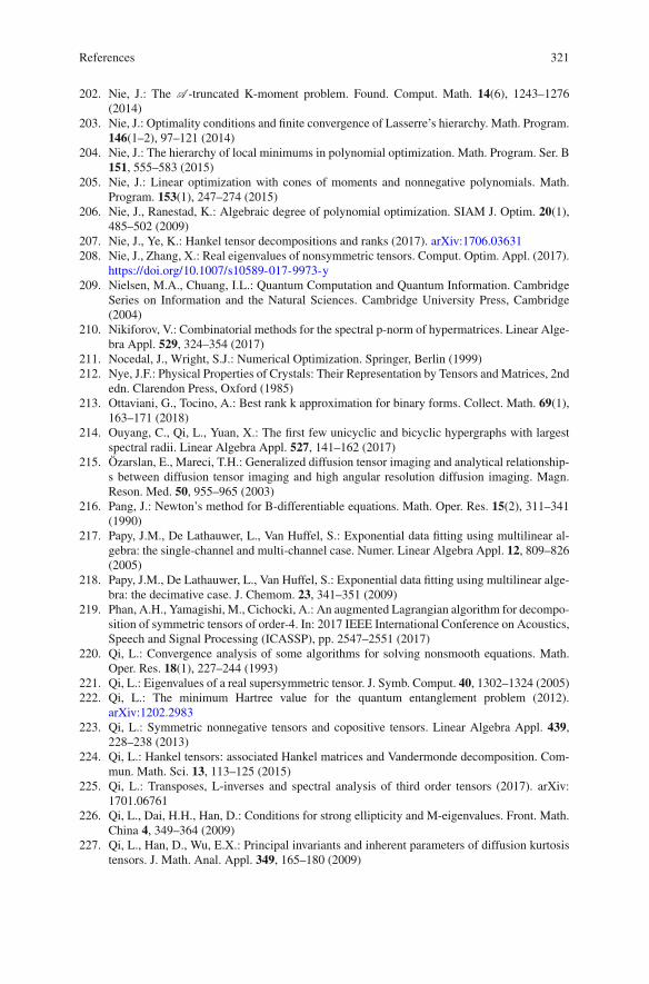
References 321
202. Nie, J.: The A -truncated K-moment problem. Found. Comput. Math. 14(6), 1243–1276(2014)
203. Nie, J.: Optimality conditions and finite convergence of Lasserre’s hierarchy. Math. Program.146(1–2), 97–121 (2014)
204. Nie, J.: The hierarchy of local minimums in polynomial optimization. Math. Program. Ser. B151, 555–583 (2015)
205. Nie, J.: Linear optimization with cones of moments and nonnegative polynomials. Math.Program. 153(1), 247–274 (2015)
206. Nie, J., Ranestad, K.: Algebraic degree of polynomial optimization. SIAM J. Optim. 20(1),485–502 (2009)
207. Nie, J., Ye, K.: Hankel tensor decompositions and ranks (2017). arXiv:1706.03631208. Nie, J., Zhang, X.: Real eigenvalues of nonsymmetric tensors. Comput. Optim. Appl. (2017).
https://doi.org/10.1007/s10589-017-9973-y209. Nielsen, M.A., Chuang, I.L.: Quantum Computation and Quantum Information. Cambridge
Series on Information and the Natural Sciences. Cambridge University Press, Cambridge(2004)
210. Nikiforov, V.: Combinatorial methods for the spectral p-norm of hypermatrices. Linear Alge-bra Appl. 529, 324–354 (2017)
211. Nocedal, J., Wright, S.J.: Numerical Optimization. Springer, Berlin (1999)212. Nye, J.F.: Physical Properties of Crystals: Their Representation by Tensors and Matrices, 2nd
edn. Clarendon Press, Oxford (1985)213. Ottaviani, G., Tocino, A.: Best rank k approximation for binary forms. Collect. Math. 69(1),
163–171 (2018)214. Ouyang, C., Qi, L., Yuan, X.: The first few unicyclic and bicyclic hypergraphs with largest
spectral radii. Linear Algebra Appl. 527, 141–162 (2017)215. Özarslan, E., Mareci, T.H.: Generalized diffusion tensor imaging and analytical relationship-
s between diffusion tensor imaging and high angular resolution diffusion imaging. Magn.Reson. Med. 50, 955–965 (2003)
216. Pang, J.: Newton’s method for B-differentiable equations. Math. Oper. Res. 15(2), 311–341(1990)
217. Papy, J.M., De Lathauwer, L., Van Huffel, S.: Exponential data fitting using multilinear al-gebra: the single-channel and multi-channel case. Numer. Linear Algebra Appl. 12, 809–826(2005)
218. Papy, J.M., De Lathauwer, L., Van Huffel, S.: Exponential data fitting using multilinear alge-bra: the decimative case. J. Chemom. 23, 341–351 (2009)
219. Phan, A.H., Yamagishi, M., Cichocki, A.: An augmented Lagrangian algorithm for decompo-sition of symmetric tensors of order-4. In: 2017 IEEE International Conference on Acoustics,Speech and Signal Processing (ICASSP), pp. 2547–2551 (2017)
220. Qi, L.: Convergence analysis of some algorithms for solving nonsmooth equations. Math.Oper. Res. 18(1), 227–244 (1993)
221. Qi, L.: Eigenvalues of a real supersymmetric tensor. J. Symb. Comput. 40, 1302–1324 (2005)222. Qi, L.: The minimum Hartree value for the quantum entanglement problem (2012).
arXiv:1202.2983223. Qi, L.: Symmetric nonnegative tensors and copositive tensors. Linear Algebra Appl. 439,
228–238 (2013)224. Qi, L.: Hankel tensors: associated Hankel matrices and Vandermonde decomposition. Com-
mun. Math. Sci. 13, 113–125 (2015)225. Qi, L.: Transposes, L-inverses and spectral analysis of third order tensors (2017). arXiv:
1701.06761226. Qi, L., Dai, H.H., Han, D.: Conditions for strong ellipticity and M-eigenvalues. Front. Math.
China 4, 349–364 (2009)227. Qi, L., Han, D., Wu, E.X.: Principal invariants and inherent parameters of diffusion kurtosis
tensors. J. Math. Anal. Appl. 349, 165–180 (2009)

322 References
228. Qi, L., Luo, Z.: Tensor Analysis: Spectral Theory and Special Tensors. SIAM, Philadelpia(2017)
229. Qi, L., Wang, Y., Wu, E.X.: D-eigenvalues of diffusion kurtosis tensors. J. Comput. Appl.Math. 221, 150–157 (2008)
230. Qi, L., Xu, C., Xu, Y.: Nonnegative tensor factorization, completely positive tensors, and ahierarchical elimination algorithm. SIAM J. Matrix Anal. Appl. 35(4), 1227–1241 (2014)
231. Qi, L., Yu, G., Wu, E.X.: Higher order positive semi-definite diffusion tensor imaging. SIAMJ. Imaging Sci. 3, 416–433 (2010)
232. Qi, L., Yu, G., Xu, Y.: Nonnegative diffusion orientation distribution function. J. Math. Imag-ing Vis. 45, 103–113 (2013)
233. Qi, L., Zhang, G., Braun, D., Bohnet-Waldraff, F., Giraud, O.: Regularly decomposable tensorsand classical spin states. Commun. Math. Sci. 15, 1651–1665 (2017)
234. Rheinboldt, W.C.: Methods for Solving Systems of Nonlinear Equations. CBMS-NSF Re-gional Conference Series in Applied Mathematics, vol. 70, 2nd edn. Society for Industrialand Applied Mathematics (SIAM), Philadelphia (1998)
235. Rockafellar, R.T.: Convex Analysis. Princeton University Press, Princeton (1970)236. Rosakis, P.: Ellipticity and deformations with discontinuous gradients in finite elastostatics.
Arch. Rational Mech. Anal. 109, 1–37 (1990)237. Sang, C., Zhao, J.: A new eigenvalue inclusion set for tensors with its applications. Cogent
Math. 4(1), 1320831 (2017)238. Schnabel, R.B., Frank, P.D.: Tensor methods for nonlinear equations. SIAM J. Numer. Anal.
21(5), 815–843 (1984)239. Schultz, T., Fuster, A., Ghosh, A., Deriche, R., Florack, L., Lim, L.: Higher-order tensors
in diffusion imaging. In: Westin, C.F., Vilanova, A., Burgeth, B. (eds.) Visualization andProcessing of Tensors and Higher Order Descriptors for Multi-valued Data, pp. 129–161.Springer, Berlin (2014)
240. Shao, J.: A general product of tensors with applications. Linear Algebra Appl. 439, 2350–2366(2013)
241. Shao, J., Yuan, X.: Some properties of the Laplace and normalized Laplace spectra of uniformhypergraphs. Linear Algebra Appl. 531, 98–117 (2017)
242. Shekhawat, H.S., Weiland, S.: A locally convergent Jacobi iteration for the tensor singularvalue problem. Multidimens. Syst. Signal Process. (2017). https://doi.org/10.1007/s11045-017-0485-9
243. Shimony, A.: Degree of entanglement. Ann. N. Y. Acad. Sci. 755, 675–679 (1995)244. Simpson, H.C., Spector, S.J.: On copositive matrices and strong ellipticity for isotropic elastic
materials. Arch. Rational Mech. Anal. 84, 55–68 (1983)245. Song, Y., Mei, W.: B tensors and tensor complementarity problems (2017). arXiv:1707.01173246. Song, Y., Qi, L.: Properties of tensor complementarity problem and some classes of structured
tensors. Ann. Appl. Math. 3, 308–323 (2017)247. Song, Y., Qi, L.: Property of some classes of structured tensors. J. Optim. Theory Appl. 165,
854–873 (2015)248. Song, Y., Qi, L.: Necessary and sufficient conditions for copositive tensors. Linear Multilinear
Algebra 63(1), 120–131 (2015)249. Song, Y., Qi, L.: Eigenvalue analysis of constrained minimization problem for homogeneous
polynomials. J. Global Optim. 64, 563–575 (2016)250. Song, Y., Qi, L.: Tensor complementarity problem and semi-positive tensors. J. Optim. Theory
Appl. 169, 1069–1078 (2016)251. Song, Y., Qi, L.: Strictly semi-positive tensors and the boundedness of tensor complementarity
problems. Optim. Lett. 11(7), 1407–1426 (2017)252. Song, Y., Qi, L.: Infinite dimensional Hilbert tensors on spaces of analytic functions. Commun.
Math. Sci. 15, 1897–1912 (2017)253. Song, Y., Yu, G.: Properties of solution set of tensor complementarity problem. J. Optim.
Theory Appl. 170, 85–96 (2016)

References 323
254. Stejskal, E.O., Tanner, J.E.: Spin diffusion measurements: spin echoes in the presence of atime-dependent field gradient. J. Chem. Phys. 42(1), 288–292 (1965)
255. Sturm, J.: Using SeDuMi 1.02, a MATLAB toolbox for optimization over symmetric cones.Optim. Methods Softw. 11(1–4), 625–653 (1999)
256. Sturmfels, B.: Tensors and their eigenvectors. Not. AMS 63(6), 604–606 (2016)257. Sun, D., Qi, L.: On NCP-functions. Comput. Optim. Appl. 13(1–3), 201–220 (1999)258. Sun, L., Zheng, B., Bu, C., Wei, Y.: Moore-Penrose inverse of tensors via Einstein product.
Linear Multilinear Algebra 64, 686–698 (2016)259. Sun, L., Zheng, B., Bu, C., Wei, Y.: Generalized inverses of tensors via a general product of
tensors. To appear in Front. Math. China (2018)260. Sun, L., Zheng, B., Zhou, J., Yan, H.: Some inequalities for the Hadamard product of tensors.
Linear Multilinear Algebra (2017). https://doi.org/10.1080/03081087.2017.1346060261. Thomson, W. (Lord Kelvin): Elements of a mathematical theory of elasticity. Philos. Trans.
R. Soc. Lond. 146, 481–498 (1856)262. Thomson, W. (Lord Kelvin): Elasticity. Encyclopedia Briannica, vol. 7, 9th edn, pp. 796–825.
Adam and Charles Black, London (1878)263. Thurston, R.N., Brugger, K.: Third-order elastic constants and the velocity of small amplitude
elastic waves in homogeneously stressed media. Phys. Rev. 133, A1604 (1964); Erratum: Phys.Rev. 135, AB3 (1964)
264. Toh, K.C., Todd, M.J., Tütüncü, R.H.: SDPT3-a MATLAB software package for semidefiniteprogramming, version 1.3. Optim. Methods Softw. 11(1–4), 545–581 (1999)
265. Tournier, J.D., Calamante, F., Gadian, D.G., Connelly, A.: Direct estimation of the fiberorientation density function from diffusion-weighted MRI data using spherical deconvolution.NeuroImage 23(3), 1176–1185 (2004)
266. Tuch, D.S.: Q-ball imaging. Magn. Reson. Med. 52, 1358–1372 (2004)267. Tuch, D.S., Reese, T.G., Wiegell, M.R., Makris, N.G., Belliveau, J.W., Wedeen, V.J.: High an-
gular resolution diffusion imaging reveals intravoxel white matter fiber heterogeneity. Magn.Reson. Med. 48, 454–459 (2002)
268. Van Huffel, S., Chen, H., Decanniere, C., Van Hecke, P.: Algorithm for time-domain NMRdata fitting based on total least squares. J. Magn. Reson. Ser. A 110, 228–237 (1994)
269. Varga, R.: Matrix Iterative Analysis, 2nd edn. Springer, Berlin (2000)270. Virga, E.G.: Octupolar order in two dimensions. Eur. Phys. J. E 38, 63 (2015)271. Walton, J.R., Wilber, J.P.: Sufficient conditions for strong ellipticity for a class of anisotropic
materials. Int. J. Nonlinear Mech. 38, 441–455 (2003)272. Wang, F., Sun, D., Zhao, J., Li, C.: New practical criteria for H-tensors and its application.
Linear Multilinear Algebra 65(2), 269–283 (2017)273. Wang, G., Zhou, G., Caccetta, L.: Z-eigenvalue inclusion theorems for tensors. Discret. Contin.
Dyn. Syst. Ser. B 22(1), 187–198 (2017)274. Wang, M., Duc, K.D., Fischer, J., Song, Y.S.: Operator norm inequalities between tensor
unfoldings on the partition lattice. Linear Algebra Appl. 520, 44–66 (2017)275. Wang, Q., Li, G., Qi, L., Xu, Y.: New classes of positive semi-definite Hankel tensors. Minimax
Theory Appl. 2(2), 231–248 (2017)276. Wang, Y., Aron, M.: A reformulation of the strong ellipticity conditions for unconstrained
hyperelastic media. J. Elast. 44, 89–96 (1996)277. Wang, Y., Huang, Z., Bai, X.: Exceptionally regular tensors and tensor complementarity
problems. Optim. Methods Softw. 31, 815–828 (2016)278. Wang, Y., Huang, Z., Qi, L.: Global uniqueness and solvability of tensor variational inequal-
ities. J. Optim. Theory Appl. (2018). https://doi.org/10.1007/s10957-018-1233-5279. Wang, Y., Qi, L., Luo, S., Xu, Y.: An alternative steepest direction method for the optimization
in evaluating the geometric discord. Pac. J. Optim. 10, 137–150 (2014)280. Wang, Y., Qi, L., Zhang, X.: A practical method for computing the largest M-eigenvalue of a
fourth-order partially symmetric tensor. Numer. Linear Algebra Appl. 16, 589–601 (2009)281. Wang, Y., Wang, G.: Two S-type Z-eigenvalue inclusion sets for tensors. J. Inequal. Appl.
2017(1), 152 (2017)

324 References
282. Wang, Y.J., Zhou, G.L.: A hybrid second-order method for homogenous polynomial opti-mization over unit sphere. J. Oper. Res. Soc. China 5(1), 99–109 (2017)
283. Wang, Y., Zhou, G., Caccetta, L.: Nonsingular H-tensors and their criteria. J. Ind. Manag.Optim. 12, 1173–1186 (2016)
284. Wei, T.C., Goldbart, P.M.: Geometric measure of entanglement and applications to bipartiteand multipartite quantum states. Phys. Rev. A 68(4), 042307 (2003)
285. Wei, Y., Ding, W.: Theory and Computation of Tensors: Multi-dimensional Arrays. AcademicPress, Amsterdam (2016)
286. Weldeselassie, Y.T., Barmpoutis, A., Atkins, M.S.: Symmetric positive semi-definite cartesiantensor fiber orientation distributions (CT-FOD). Med. Image Anal. 16(6), 1121–1129 (2012)
287. Wiant, D., Neupane, K., Sharma, S., Gleeson, J.T., Sprunt, S., Jákli, A., Pradhan, N., Iannac-chione, G.: Observation of a possible tetrahedratic phase in a bent-core liquid crystal. Phys.Rev. E 77, 061701 (2008)
288. Wu, E.D., Cheung, M.M.: MR diffusion kurtosis imaging for neural tissue characterization.NMR Biomed. 23, 836–848 (2010)
289. Xiang, H., Qi, L., Wei, Y.: A note on the M-eigenvalues of the elasticity tensor and strongellipticity (2017). arXiv:1708.04876
290. Xiao, P., Wang, L., Lu, Y.: The maximum spectral radii of uniform supertrees with givendegree sequences. Linear Multilinear Algebra 523, 33–45 (2017)
291. Xie, Z.J., Jin, X.Q., Wei, Y.M.: Tensor methods for solving symmetric M-tensor systems. J.Sci. Comput. 74(1), 412–425 (2018)
292. Yang, Q., Yang, Y.: Further results for Perron-Frobenius theorem for nonnegative tensors II.SIAM J. Matrix Anal. Appl. 32, 1236–1250 (2011)
293. Yang, S.D.: Description of second-order three-dimensional magnetic neutral points. Phys.Plasmas 24(1), 012903 (2017)
294. Yang, W.W., Ni, Q.: A cubically convergent method for solving the largest eigenvalue of anonnegative irreducible tensor. Numer. Algorithms (2017). https://doi.org/10.1007/s11075-017-0358-1
295. Yang, Y., Feng, Y., Huang, X., Suykens, J.A.K.: Rank-1 tensor properties with applicationsto a class of tensor optimization problems. SIAM J. Optim. 26, 171–196 (2016)
296. Yang, Y., Yang, Q.: Further results for Perron-Frobenius theorem for nonnegative tensors.SIAM J. Matrix Anal. Appl. 31, 2517–2530 (2010)
297. You, L., Chen, Y., Yuan, P.: Some results of strongly primitive tensors (2017). arX-iv:1705.04554
298. Yu, G., Song, Y., Xu, Y., Yu, Z.: Spectral projected gradient methods for generalized tensoreigenvalue complementarity problem (2016). arXiv:1601.01738
299. Yu, G., Yu, Z., Xu, Y., Song, Y., Zhou, Y.: An adaptive gradient method for computinggeneralized tensor eigenpairs. Comput. Optim. Appl. 65(3), 781–797 (2016)
300. Yuan, P., You, L.: Some remarks on P, P0, B and B0 tensors. Linear Algebra Appl. 459,511–521 (2014)
301. Yue, J.J., Zhang, L.P., Lu, M., Qi, L.Q.: The adjacency and signless Laplacian spectra of coredhypergraphs and power hypergraphs. J. Oper. Res. Soc. China 5(1), 27–43 (2017)
302. Zhang, F., Zhou, B., Peng, L.: Detecting local illumination using skewness of oriented gradi-ents from a single image. Appl. Mech. Mater. 58, 2381–2386 (2011)
303. Zhang, F., Zhou, B., Peng, L.: Dynamic texture analysis using eigenvectors of gradient skew-ness tensors. In: 2012 International Conference on Computer Science and Service System(CSSS). IEEE (2012)
304. Zhang, F., Zhou, B., Peng, L.: Gradient skewness tensors and local illumination detection forimages. J. Comput. Appl. Math. 237, 663–671 (2013)
305. Zhang, L., Qi, L., Zhou, G.: M-tensors and some applications. SIAM J. Matrix Anal. Appl.35, 437–452 (2014)
306. Zhang, W., Kang, L., Shan, E., Bai, Y.: The spectra of uniform hypertrees. Linear AlgebraAppl. 533, 84–94 (2017)
References 325
307. Zhang, W., Liu, L., Kang, L., Bai, Y.: Some properties of the spectral radius for generalhypergraphs. Linear Algebra Appl. 513, 103–119 (2017)
308. Zhang, X., Ling, C., Qi, L., Wu, E.X.: The measure of diffusion skewness and kurtosis inmagnetic resonance imaging. Pac. J. Optim. 6, 391–404 (2010)
309. Zhang, X., Qi, L.: The quantum eigenvalue problem and Z-eigenvalues of tensors (2012).arXiv:1205.1342
310. Zhang, X., Zhou, G., Caccetta, L., Alqahtani, M.: Approximation algorithms for nonnegativepolynomial optimization problems over unit spheres. Front. Math. China 12(6), 1409–1426(2017)
311. Zhao, J.: A new Z-eigenvalue inclusion theorem for tensors (2017). arXiv:1705.05187312. Zhao, J.: A tighter Z-eigenvalue localization set for tensors and its applications (2017).
arXiv:1704.03707313. Zhao, J., Li, C.: Singular value inclusion sets for rectangular tensors. Linear Multilinear
Algebra (2017). https://doi.org/10.1080/03081087.2017.1351518314. Zhao, J., Sang, C.: A new S-type upper bound for the largest singular value of nonnegative
rectangular tensors. J. Inequal. Appl. 2017(1), 105 (2017)315. Zhao, N., Yang, Q., Liu, Y.: Computing the generalized eigenvalues of weakly symmetric
tensors. Comput. Optim. Appl. 66(2), 285–307 (2017)316. Zhao, R., Zheng, B., Liang, M.: On the estimates of the Z-eigenpair for an irreducible non-
negative tensor. J. Math. Anal. Appl. 450(2), 1157–1179 (2017)317. Zhou, J., Sun, L., Wei, Y., Bu, C.: Some characterizations of M-tensors via digraphs. Linear
Algebra Appl. 495, 190–198 (2016)318. Zou, W., He, Q., Huang, M., Zheng, Q.: Eshelby’s problem of non-elliptical inclusions.
J. Mech. Phys. Solids 58, 346–372 (2010)319. Zubov, L.M., Rudev, A.N.: On necessary and sufficient conditions of strong ellipticity of
equilibrium equations for certain classes of anisotropic linearly elastic materials. ZAMM-J. Appl. Math. Mech. 96(9), 1096–1102 (2016)

Index
AAcoustic tensor, 258Anti-circulant tensor, 50Apparent kurtosis coefficient, 186Archimedean, 170
BBent-core liquid crystal, 208Best rank one approximation, 4Bi-block symmetric tensor, 278Buckingham’s formula, 226
CCayley transform, 54CB-eigenpair, 172CB-eigenvalue, 172CB-eigenvector, 172C-eigenvalue, 208, 216Centrally anti-symmetry, 212Characteristic polynomial, 4Classical spin state, 301Combinatorial eigenpair, 172Combinatorial eigenvalue, 172Combinatorial eigenvector, 172Completely decomposable tensor, 300Cone eigenvalue, 136Converse piezoelectric effect, 207, 223Copositive function, 68Copositive tensor, 80Cyclically symmetry, 213
DD-eigenvalue, 186Diagonal face tensor, 35
Diagonalizable tensor, 81Diagonal tensor, 2Diffusion Kurtosis Imaging (DKI), 186Diffusion kurtosis tensor, 183, 186Diffusion tensor, 185Diffusion Tensor Imaging (DTI), 184d-regular mapping, 69
EE-characteristic polynomial, 5, 208, 234E-eigenvalue, 5E-eigenvector, 5Eigenconfiguration, 244Eigendiscriminant, 244Eigenvalue, 4Eigenvector, 4Elasticity, 251Elasticity tensor, 249, 250Elasticity Z-tensor, 267Elastic modulus, 251Entanglement eigenvalue, 286, 292, 298ER-tensor, 127Exceptionally regular function, 126Exponential data fitting, 60
FFractional anisotropy, 185Fractional kurtosis anisotropy, 188Frobenius norm, 2Funk–Radon transformation, 196
GGauss–Seidel method, 37Generalized diffusion tensor, 191
© Springer Nature Singapore Pte Ltd. 2018L. Qi et al., Tensor Eigenvalues and Their Applications, Advances in Mechanicsand Mathematics 39, https://doi.org/10.1007/978-981-10-8058-6
327
328 Index
Generalized eigenvalue, 171Generalized eigenvector, 171Generating vector, 50Geometric measure, 285, 289GUS-property, 67, 122
HH+-eigenvalue, 148H++-eigenvalue, 148H-eigenvalue, 4Hadmard product, 172Hankel tensor, 50Harmonic function, 243Hartree value, 285Higher order diffusion tensor, 183Homotopy method, 22Hooke’s law, 250H-tensor, 10Hypermatrix, 1
IIdentical singular pair, 143Identity tensor, 2Invariant, 6
JJacobi method, 37
KK-eigenvalue, 137, 159K-eigenvector, 137, 159Kernel tensor, 207, 213K-regular, 159Kronecker product, 267K-spectrum, 137
LLaplace operator, 243Left-side anti-symmetry, 212Left-side symmetry, 212L-eigenvalue, 207L-eigenvalue decomposition, 215L-eigenvalue of tensors, 215Levi-Civita tensor, 212, 217L-inverse, 207L-inverse of tensors, 213Liquid crystal, 208Łojasiewicz property, 58Lower half tensor, 35
MMagnetic resonance imaging, 184Mean diffusivity, 185Mean kurtosis, 187M-eigenvalue, 249M-equation, 11Minimum Hartree value, 290Mixed state, 286M-positive definite, 249M-tensor, 10Multilinear game, 72Multilinear system, 9
NNash equilibrium, 65NCP-function, 152Nonsingular M-tensor, 10Nonsingular tensor, 212Null space, 210Null space of a tensor, 215
OOctupolar potential, 228Octupolar tensor, 208, 226Orthogonal tensor, 211, 213Orthogonally similar, 6
PP′-tensor, 91P′
0-tensor, 91P0-tensor, 84P-function, 70Paired symmetric tensor, 274Pareto-eigenvalue, 136, 137, 159Pareto-eigenvector, 137, 159Pareto H-eigenvalue, 148Pareto Z-eigenvalue, 148Pareto-spectrum, 137Partial Z-tensor, 111Permutation tensor, 212Piezoelectric effect, 207, 222Piezoelectric tensor, 208Piezoelectric-type tensor, 218P0-function, 106Positive definite, 3Positive semi-definite, 3P-tensor, 84Pure state, 286

Index 329
QQ-ball imaging, 195Q-tensor, 98Quantum eigenvalue, 292Quantum entanglement, 287Quantum satellite, 287
RRank-one tensor, 2Regularly decomposable tensor, 286, 300Resultant, 4, 231Resultant theory, 208Rhombic system, 259Right-side anti-symmetry, 212Right-side symmetry, 212R0-tensor, 98R-tensor, 98
SSemi-paired symmetric tensor, 281Semi-positive tensor, 92Semismooth function, 151Singular value of a tensor, 216Skewness, 203SOR method, 37S0-tensor, 117Spectral hypergraph theory, 7Spectral radius, 10Spherical deconvolution, 199Spherical harmonics, 196Spin state, 286S-positive definiteness, 254S-positive semi-definiteness, 254SP0-tensor, 106S-tensor, 117Strain tensor, 250Stress tensor, 250Strict K-eigenvalue, 137Strict Pareto-eigenvalue, 137Strictly copositive function, 68Strictly copositive tensor, 80Strictly lower half tensor, 35Strictly semi-positive tensor, 92Strictly upper half tensor, 35Strong ellipticity, 249Strong P0-tensor, 106
Strongly copositive function, 68Strongly paired symmetric tensor, 274Strongly semismooth function, 151Strong P-tensor, 125Support, 1Symmetric rank-one tensor, 2Symmetric tensors, 1Symmetric traceless tensor, 208
TTensor, 1Tensor complementarity problem, 65Tensor eigenvalue complementarity prob-
lem, 135Tensor generalized eigenvalue complemen-
tarity problem, 135Tensor higher-degree eigenvalue comple-
mentarity problem, 136Tensor inner product, 2Tensor outer product, 2Tesor decomposition, 49, 281Totally anti-symmetry, 212Trace, 210Traceless tensor, 226, 227Transpose of a third order tensor, 207Transpose tensor, 213Triangular equation, 17
UU-eigenvalue, 286Unfolded matrix, 280Uniform P-function, 70Unitary eigenvalue, 297Unitary symmetric eigenvector, 298Upper half tensor, 35US-eigenvalue, 286
ZZ+-eigenvalue, 148Z++-eigenvalue, 148Z-eigenvalue, 5, 216Z-eigenvector, 5Z-function, 69Zero tensor, 1Z-tensor, M-tensor, H-tensor, 10