Liquidity Traps and Monetary Policy: Managing aCredit Crunch

Francisco Buera ∗ Juan Pablo Nicolini †‡

June 11, 2013

Abstract

We present a model of a monetary economy with heterogeneous producers andcollateral constraints. We use the model to study the consequences of alternativemonetary policies following a tightening in the collateral requirement. Firstly, weshow that when policy does non react to the change in the environment, thereis a large deflation, and a particularly severe contraction in an economy withnominal private debt. Secondly, we consider a monetary policy that implementsa constant inflation target. Price stability imposes a bound on the real interestrate and it requires a sharp increase in the supply of assets by the government,moving the economy into a liquidity trap and crowding out private investment.In this case the credit crunch leads to a less pronounced recession, but slowerrecovery. Finally, we show that the welfare consequences of alternative monetarypolicies vary substantially across individuals.

∗University of California at Los Angeles and NBER; fjbuera@econ.ucla.edu.†Federal Reserve Bank of Minneapolis and Universidad Di Tella; juanpa@minneapolisfed.org.‡The views expressed in this paper do not represent the Federal Reserve Bank of Minnespolis or

the Federal Reserve System.

1

1 Introduction

The year 2008 will be remembered in the macroeconomics literature for long. This isso, not only because of the massive shock that hit global financial markets, particu-larly since the bankruptcy of Lehman and the collapse of the interbank market thatimmediately followed, but also because of the unusual and extraordinary response toit, emanated from all mayor Central Banks. The reaction of the Fed is a clear example:it doubled its balance sheet in just three months - from 800 billion on September 1st,to 1,6 trillion by December 1st. Then, it kept on increasing it to reach around 3 trillionby the end of 2012.1 Very similar measures where taken by the European Central Bankand other Central Banks of developed economies. We guess that most macroeconomistwould agree with the notion that the 2008-2013 period is, from the point of view ofmacroeconomic theory and policy, among the most dramatic ones in twentieth centuryhistory, perhaps second only to the Great Depression period.

Paradoxically, however, none of the models used by Central Banks at the timein developed economies was of any use to study neither the financial shock, nor thereaction of monetary policy. Those models essentially ignore financial markets on onehand, and monetary aggregates on the other. There were good reasons for this: byand large, big financial shocks seemed to belong exclusively to emerging economiessince the turbulent 1930’s. We are not sure how to define emerging economies, butalways had the sense that it meant highly volatile financial markets. According tothis narrow definition, it seems that 2008 taught us, among other things, that we livein an emerging world.2 In addition, monetary economics developed, in the last twodecades, around the Central Bank rhetoric of emphasizing exclusively on the shortterm nominal interest rate. Measures of liquidity or money, were completely ignoredas a stance of monetary policy; one of the reasons being that empirical relationshipsbetween monetary aggregates, interest rates and prices, that stood well for most of thetwentieth century, broke down in the midst of the banking deregulation that startedin the 1980’s.3 Consequently, there is a lack of general equilibrium models that can beused to study the effects of monetary policies like the Fed adopted since 2008, duringtimes of financial distress. The purpose of this paper is to provide one such modeland study the macroeconomic effects of monetary policy during a credit crunch. Westudy a model with heterogenous entrepreneurs that face cash-in-advance constraintson purchases and collateral constraints on borrowing. The collateral constraints giverise to a non-trivial financial market. The cash-in-advance constraints give raise to amoney market. We use this model to study the effect of alternative monetary policiesin the equilibrium allocation following a shock to financial intermediation.

An essential role of financial markets is to reallocate capital from wealthy individualswith no profitable investment project - savers - to individuals with profitable projects

1Compare it with 1987, 2000 (Y2K) and 2001 (9-11).2See Diaz-Alejandro (1985) for a very interesting view on the subject.3For a detailed discussion of this, and a reinterpretation of the evidence that strongly favors the

view of a stable ”money demand” relationship, see Lucas and Nicolini (2013).

2

and no wealth - investors. The efficiency of these markets determines the equilibriumallocation of physical capital across projects and therefore equilibrium intermediationand total output.

The development literature has study models of the financial sector with theseproperties, the key friction being an exogenous collateral constraint on investors. Weborrow the model of financial markets from that literature. The equilibrium allocationcritically depends on the nature of the collateral constraints; the tighter the constraints,the less efficient the allocation of capital and the lower are total factor productivityand output. A tightening of the collateral constraint creates disintermediation anda recession. This reduction in the ability of financial markets to properly performthe allocation of capital across projects, we interpret as a negative financial shock.We view this as a sector specific technology shock with, as we will argue, aggregateconsequences.

The single modification we introduce to this nowadays standard model in the de-velopment literature, is a cash-in-advance constraint on households. While we brieflydiscuss the case with nominal wage rigidity at several points, we assume prices andwages to be fully flexible, mostly to highlight the effects that are novel in the model.Monetary policy determines equilibrium inflation and nominal interest rates and it hasreal effects. This is so because of the usual well understood distortionary effects ofinflation in a cash-credit world, but, more importantly, because of the zero bound onnominal interest rates restriction that arises from optimizing behavior of individualsin the model. The analysis of the effect of monetary policy at the zero bound is thecontribution of this paper.

One attractive feature of the financial sector model we use, is that in the recessionthat follows a shock to the collateral constraint, the equilibrium real interest rate goesdown for several periods.4 The reason is that savings must be reallocated to lowerproductivity entrepreneurs, but they will only be willing to do it for a lower interestrate. To put it differently, the ”demand” for loans falls, and this pushes down thereal interest rate. If the shock is large enough, the equilibrium interest rate becomesnegative. Depending on what monetary policy does, the bound on the nominal interestrate may become a bound on the real interest rate. As an example, imagine a monetarypolicy that targets, successfully, a constant price level: If inflation is zero, the Fisherequation, which is an equilibrium condition of the model, implies a zero lower boundon the real interest rate. The way the negative real interest rate interacts with the zerobound on nominal interest rates that arises in a monetary economy, under alternativemonetary policies, is at the hearth of the mechanism discussed in the paper.

The qualitative properties of the recession generated by a tightening of the collateralconstraint, or credit crunch, are in line with some of the events that unfolded since2008, like the persistent negative real interest rate, the sustained periods with theeffective zero bound on nominal interest rates and the substantial drop in investment.

4This feature is special of the credit crunch. If the recession is driven by an equivalent, butexogenous, negative productivity shock, the real interest rate remains positive, as we will show.

3

In addition, the model is consistent with the very large increases in liquidity whilethe zero bound binds. Thus, we argue, the model in the paper is a good candidateto interpret the way monetary policy is affecting the economy nowadays. Some - butnot all! - features of this great contraction make it a - distant - cousin of the greatdepression of the 30’s. The great depression evolved in parallel to a mayor bankingcrisis and the severity of the depression was unique in US history. The role of monetarypolicy has also been at the center of the debate: For many, the unresponsive Fed playeda key role in the unfolding of events during the great depression.5 A strongly held viewattributes the reaction of the Fed in September 2008 to the lessons that Friedmanand Schwartz draw from the great depression and attributes to the policy reaction theavoidance of an even major recession.

We first study the case in which the monetary authority is irresponsive to the creditcrunch and does not change policy. The model implies that the nominal interest ratewill be at its zero bound for a finite number of periods and there will be a deflation onimpact. To the extent that debt obligations are in nominal terms, this deflation stronglyaccentuates the recession well beyond the one generated by the credit crunch, due to adebt deflation problem. We then study active inflation targeting policies, for low valuesof the inflation target. In these case, the deflation and the associated debt deflationproblem are avoided by a very large increase in the supply of government liabilities,that must follow the credit crunch. Was the different monetary policy recently adopted,the reason why the great contraction was much less severe than the great depression?Our model suggests this may well be the case.6

The number of periods that the economy will be a the zero bound and the amountof liquidity that must be injected depends on the target for the rate of inflation. Theevolution of output critically depends on this too. As we mentioned above, the inter-action between the inflation target and the zero bound on nominal interest rates is thekey to understand the mechanism. Imagine, as before, that the target for inflation iszero. Thus, the Fisher equation plus the zero bound constraint imply that the realinterest rate cannot be negative. This imposes a floor on how low can the real interestrate be. But for this to be an equilibrium, private savings must end up somewhere else:This is the role of government liabilities. In this heterogeneous credit-constraint agentsmodel, debt policy does have effects on equilibrium interest rates, even if taxes arelump-sum. Thus, the issuance of government liabilities crowds out private investment.

But there is an additional effect of monetary policy. In the model, a credit crunchgenerates a recession because total factor productivity falls. The reason, as we men-tioned above, is that capital needs to be reallocated from high productivity entrepreneurs

5See Friedman and Schwartz (1963)6Friedman and Schwartz argued that the Fed should have increased substantially its balance sheet

in order to avoid the deflation during the great depression. In 2002, Bernanke, then a Federal ReserveBoard governor, said in a speech in a conference to celebrate Friedman’s 90th birthday, “I would liketo say to Milton and Anna: Regarding the Great Depression. You’re right, we did it. We’re verysorry. But thanks to you, we won’t do it again.” Bernanke’s speech has been published in The GreatContraction, 1929-1933: (New Edition) (Princeton Classic Editions), 2008.

4

for which the collateral constraint binds, and therefore must de-leverage, to low pro-ductivity entrepreneurs for which the collateral constraint does not bind. As a resultof the drop in productivity, output and investment fall, at the same time that finan-cial intermediation shrinks. Therefore, by keeping real interest rates high, an inflationtargeting policy leaves the most unproductive entrepreneurs out of production, increas-ing average productivity. Thus, a target for inflation, if low, implies that the drop inproductivity will be lower than in the real economy benchmark - there will be lessreallocation of capital to low productivity workers - but the recession will be moreprolonged - capital accumulation falls because of the crowding out effect. If the targetfor inflation is higher, say 1%, then the effective lower bound on the real interest rate is-1%, lower than before. Thus, the amount of government liabilities that must be issuedwill be smaller, the crowding out will be smaller, but the drop in average productivitywill be higher.

The model provides an interpretation of the after 2009 events that is different fromthe one provided by a branch of the literature that, using New Keynesian models,places a strong emphasis on the interaction between the zero bound constraint onnominal interest rates and price rigidities.7 This is also the dominant view of monetarypolicy at mayor central banks, including the Fed. According to this view, a shock -often associated to a shock in the efficiency of intermediation 8- drove the natural realinterest rate to negative values. The optimal monetary policy in those models is to setthe nominal interest rate equal to the natural real interest rate. However, due to thezero bound, that is not possible. But it is optimal, unambiguously, to keep the nominalinterest rate at the zero bound, as the Fed has been doing for over 4 years now. Themodel we study stresses a different and novel trade-off between ameliorating the initialrecession and delaying the recovery.9 When the central bank chooses a lower inflationtarget, the real interest rate is constrained to be higher, and therefore, there is lessreallocation of capital toward less productive, and previously inactive, entrepreneurs.The counterpart of the milder drop in TFP is a drop in investment due to the crowdingout, leading to a substantial and persistence decline in the stock of capital.

As in the recent experience, to maintain price stability during a credit crunch thegovernment needs to expand dramatically the size of its liabilities. In a credit crunchthe capacity of productive entrepreneurs to supply bonds is reduced, resulting in anexcess demand of saving instruments by unproductive entrepreneurs and workers. Thisis, obviously, a demand for real assets. Without any policy intervention, the adjustment

7See Christiano et al. (2011), Correia et al. (forthcoming), Eggertsson (2011),Eggertsson and Wood-ford (2003), Krugman (1998), Werning (2011) and references therein.

8See for example Curdia and Eggertsson (2009), Drautzburg and Uhlig (2011), and Galı et al.(2011).

9We consider a model with flexible prices in order to more clearly focus on the novel mechanisms inour paper. However, it is straightforward to extend our analysis and allow for wage rigidity. Nominalwage rigidity would make the recession even stronger in the case of the unresponsive monetary policydue to the ensuing deflation. The effect of nominal wage rigidity will be small in the case of inflationtargeting. In any case, the trade-off discussed in the text will remain.

5

must come about through a deflation. To avoid the deflation induced by the excessdemand of mediums to ”store value”, the government must increase the supply ofmoney - or government bonds, which at the zero bound are perfect substitutes. Ontop of this, the increase in the supply of government bonds induces a further increasein the demand of these bonds by unconstrained entrepreneurs, as these agents save inanticipation of the higher taxes that will be raised to pay the interest of this debt.

The paper proceeds as follows. In Section 2, we present the model and solve theindividual’s problems. In Section 3, define an equilibrium and partially characterizethe equilibrium dynamics. In Section 4, we solve numerically the model under alterna-tive monetary policies and discuss the results. We discuss the distribution of welfareconsequences of alternative monetary policies in Section 5

2 The Model

In this section we describe the model, that follows closely the framework in Moll (2012).The model’s attractive feature for our purposes is that it explicitly deals with heteroge-neous agents that are subject to collateral constraints in a relatively tractable fashion.This model has been used to the characterize the aggregate implications of a creditcrunch, generated by a drop in the amount of credit that can be obtained from eachunit of capital posed as collateral (Buera and Moll, 2012). We modify the originalmodel by imposing a cash-in-advance constraint on consumer’s decision problem. Thisallows us to study the effect of alternative monetary policies following a credit crunch.

We analyze a deterministic economy and assume that starting at the steady state,at time zero all agents learn that the collateral will be tightened for a finite number ofperiods. We then explore the effects of alternative monetary policies. In each case, weassume agents have perfect foresight regarding the evolution of the collateral constraintand of monetary policy.

2.1 Households

All agents have identical preferences, given by

∞∑t=0

βt[ν log ci1t + (1− ν) log ci2t

](1)

where ci1t and ci1t are consumption of the cash good and of the credit good, for agenti at time t, and β < 1. The assumption of logarithmic preferences implies a simpleexpression for the agents wealth accumulation decision.

Each agent also faces a cash-in-advance constraint of the type

ci1t ≤mit

pt. (2)

6

where mit is the beginning of period money holdings and pt is the money price of

consumption at time t.The economy is inhabited by two classes of agents, a mass L of workers and a

mass 1 of entrepreneurs. In addition, entrepreneurs are heterogeneous with respect totheir productivity z ∈ Z. We assume that the productivity is constant through theirlifetime. We let Ψ(z) be the measure of entrepreneurs of type z. We proceed now tostudy the optimal decision problems of entrepreneurs and households.

Entrepreneurs Each entrepreneur starts every period managing an active firm ornot, and given financial wealth - capital plus bonds - and money holdings, and mustdecide, at the end of each period, whether to be active in the following period, and if so,how much capital to invest in her own firm. An entrepreneur’s investment is constraintby her own non-monetary resources at the end of the period a and the amount of bondsshe can sell −b, k ≤ −b + a, where we assume that decision to be limited by a simplecollateral constraint of the form

−bi ≤ θki, (3)

for some exogenously given θ ∈ [0, 1).If the entrepreneur decides not to be active (to allocate zero capital to her own

firm), then she invest all her non-monetary wealth to purchase bonds.We assume that the technology available to entrepreneurs of type z is given by the

Cobb-Dougls form

y = (zk)1−αlα.

This technology implies that revenues of an entrepreneur net of labor payments is alinear function of the capital stock, %zk, where % = α ((1− α)/w)(1−α)/α is the return tothe effective units of capital zk, and w denotes the real wage. Thus, the end of periodinvestment and leverage choice of entrepreneurs with ability z solves the following linearprogram

maxk,d

%zk + (1− δ)k + (1 + r)b

k ≤ a− b,−b ≤ θk.

Denoting the maximum leverage by λ = 1/(1 − θ), it is straightforward to show thatthe optimal capital and leverage choice are given by the following policy rules, with asimple threshold property

k(z, a) =

{λa, z ≥ z

0, z < z

7

and

b(z, a) =

{−(λ− 1)a, z ≥ z

a, z < z

where z solve

%z = r + δ,

where % has been defined above.Given entrepreneurs’ optimal investment and leverage decisions, they would face a

linear return to their non-monetary wealth that is a simple function of their produc-tivity

R(z) =

{λ (%z − r − δ) + 1 + r, z > z

1 + r, z ≤ z

Given these definitions, the budget constraint of entrepreneur i, with net-worth aitand productivity zi, will be given by

ci1t + ci2t + ait+1 +mit+1

pt= Rt(z

i)ait +mit

pt− Tt(zi), (4)

where we allow lump-sum taxes (transfers if negative) to be a function of the – exoge-nous – productivity of entrepreneurs.

Note that we are adopting the timing convention of Svensson (1985), in whichgoods markets open in the morning and asset markets open in the afternoon. Thus,agents buy cash goods at time t with the money holdings they acquired at the end ofperiod t−1. Similarly, production by entrepreneurs at time t is done with capital goodsaccumulated at the end of period t−1. An advantage of this timing for our purposes isthat it treats all asset accumulation decisions symmetrically, using the standard timingfrom capital theory.

Workers Workers are all identical and are endowed with a unit of time that is in-elastically supplied to the labor market. Thus their budget constraints are given by

cW1t + cW2t + aWt+1 +mWt+1

pt= (1 + rt)a

Wt + wt +

mWt

pt− TWt (5)

where aWt+1 and mWt+1 are real financial assets and nominal money holdings chosen at

time t, and TWt are lump-sum taxes paid to the government. If TWt < 0, these representtransfers from the government to workers. We impose on workers a non-borrowingconstraint, so aWt ≥ 0 for all t.10

10This is a natural constraint to impose. It is equivalent to impose on workers the same collat-eral constraints entrepreneurs face; since in this case workers will never decide to hold capital inequilibrium.

8

2.2 Optimality conditions

The optimal problem of agents is to maximize (1) subject to (2) and (4) for en-trepreneurs or (5) for workers. Note that the only difference between the two budgetconstraints is that entrepreneurs have no labor income. For workers, as for inactiveentrepreneurs, the return to their non-monetary wealth equals 1 + rt. In what follows,to save on notation, we drop the index for individual entrepreneurs i unless strictlynecessary.

In this economy, gross savings come from inactive entrepreneurs and, potentially,from workers. Note that the return of holding real financial assets for these agents isRt(z) = (1 + rt) , while the return of holding money - ignoring the liquidity services - isgiven by pt/pt+1. Thus, if there is intermediation in equilibrium, the return of holdingmoney cannot be higher than the return of holding financial assets. If we define thenominal return as (1 + rt)

pt+1

pt, then for intermediation to be non-zero in equilibrium,

the zero bound constraint

(1 + rt)pt+1

pt− 1 ≥ 0 (6)

must hold for all t.The first order conditions of household’s problem imply the standard Euler equation

1

β

c2t+1

c2t= Rt+1, t ≥ 0, (7)

and intra-temporal optimality condition between cash and credit goods

ν

1− νc2t+1

c1t+1

= Rt+1pt+1

pt, t ≥ 1. (8)

which requires that the marginal rate of substitution between cash and credit goods attime t+ 1 equals their relative price, given by the nominal return of money.

Solving forward the period budget constraint (4), using the optimal conditions(7) and (8) for all periods, and assuming that the cash-in-advance is binding at thebeginning of period t = 0, we obtain the following solutions for consumption of thecredit good and financial assets for agents that face a strictly positive opportunity cost

9

of money in period t+ 1,11

c2t =(1− ν) (1− β)

1− ν (1− β)

[Rt(z)at −

∞∑j=0

Tt+j(z)∏js=1Rt+s(z)

]

and

at+1 = β

[Rt(z)at −

∞∑j=0

Tt+j(z)∏js=1Rt+s(z)

]+∞∑j=1

Tt+j(z)∏js=1Rt+s(z)

.

These equations characterize the solution for active entrepreneurs. Note that for them,the opportunity cost of holding money is given by Rt(z)pt+1/pt > (1 + rt) pt+1/pt ≥ 1,where the last inequality follows form the zero bound condition (6) . Thus, the cash-in-advance constraint is always binding for active entrepreneurs from time t = 1 on,even when nominal interest rates are zero. The solution also characterizes the optimalbehavior of inactive entrepreneurs, as long as (1 + rt) pt+1/pt − 1 > 0.

The solution for inactive entrepreneurs in periods in which the nominal interestrate is zero, (1 + rt) pt+1/pt − 1 = 0, is

at+1 +mt+1

pt−mTt+1

pt= β

[Rt(z)at −

∞∑j=0

Tt+j(z)∏js=1Rt+s(z)

]+∞∑j=1

Tt+j(z)∏js=1Rt+s(z)

.

where

mTt+1

pt=

ν(1− β)β

1− ν(1− β)

[Rt(z)at −

∞∑j=0

Tt+j(z)∏js=1Rt+s(z)

](9)

are the real money balances that will be used for transaction purposes in period t+ 1,and mt+1/pt − mT

t+1/pt ≥ 0 are the excess real money balances that are hoard fromperiod t to t+1. Notice that for individuals with a strictly positive opportunity cost ofmoney, Rt+1(z)pt+1/pt > 0, their cash-in-advance constraint are binding in t + 1, andtherefore, mT

t+1 = mt+1.

11Note that it could be possible that initial money holdings are so large for an active entrepreneur,that the cash-in-advance constraint will not be binding the first period. This case will not be relevantprovided initial real cash balances satisfy the following condition:

m0

p0≤ ν (1− β)

1− ν (1− β)

R0(z)a0 −∞∑j=0

Tj(z)∏js=1Rs(z)

.If this condition is not satisfy, then the optimal policy for period t = 0 is to consume a fraction ν(1−β)and (1 − ν)(1 − β) of the present value of the wealth, inclusive of the initial real money balances,in cash and credit goods. Similarly, the non-monetary wealth and real money holding at the end ofthe first period are functions of the present value of the wealth, inclusive of the initial real moneybalances.

10

The optimal policy for workers is slightly more involved, as they will tend to facebinding borrowing constraints in finite time. In particular, as long as the (1+r∞)β < 1,as it will be the case in the equilibria we will discuss, where r∞ is the real interest ratein the steady state, workers drive their wealth to zero in finite time, and are effectivelyhand-to-mouth consumers in the long run. That is, for sufficiently large t,

cW2,t =1− ν

1− ν(1− β)(wt − TWt )

and

cW1,t+1 =mWt+1

pt+1

=νβ

1− ν(1− β)

ptpt+1

(wt − TWt ).

Along a transition, workers may accumulate assets for a finite number of periods. Thiswould typically be the case if they expect a future drop in their wages, or they receivea temporarily large transfer, TWt < 0.

2.3 Demographics

The decision rules of entrepreneurs imply that the wealth of active entrepreneurs in-creases over time, while that of inactive entrepreneurs converges to zero. Thus, eachactive entrepreneur saves away from the collateral constraint asymptotically. In orderfor the model to have a non-degenerate distribution of wealth across productivity typesin a steady state, we assume that a fraction 1−γ of entrepreneurs die and are replacedby equal number of new entrepreneurs. The productivity z of the new entrepreneursis drawn from the same distribution Ψ(z), i.i.d across entrepreneurs and over time.We assume that there are no annuity markets and that each new entrepreneur inheritsthe assets of a randomly drawn dying entrepreneur. Agents do not care about futuregenerations, so if we let β be the pure discounting factor, they discount the future withthe compound factor β = βγ, which is the one we used above.

2.4 The Government

In every period the government chooses the money supply Mt+1, issues one-periodbonds Bt+1, and uses type specific lump-sum taxes (subsidies) Tt(z) and TWt . Govern-ment policies are constrained by a sequence of period by period budget constraints

Bt+1 − (1 + rt)Bt +Mt+1

pt− Mt

pt+

∫T (z)tΨ(dz) + TWt = 0. (10)

We denote by Tt the total taxes receipts of the government,

Tt =

∫Tt(z)Ψ(dz) + TWt .

11

In representative agent models, monetary policy can be executed via lump-sumtaxes and transfers that, because those models satisfy Ricardian equivalence, are neu-tral. However, in this model, Ricardian equivalence will not hold for two related rea-sons. First, agents face different rates of return to their wealth. Thus, the presentvalue of a given sequence of taxes and transfers differs across agents. Second, lump-sum taxes and transfers will redistribute wealth in general, and these redistributionsdo affect aggregate allocations, due to the presence of the collateral constraints. In thenumerical sections, we will be explicit regarding the type of transfers we consider andthe effect they have on the equilibrium allocation.

3 Equilibrium

Given sequences of government policies {Mt, Bt, Tt}∞t=0 and collateral constraints {θt}∞t=0,an equilibrium is given by sequences of prices {rt, wt, pt}∞t=0, and corresponding quan-tities such that:

• Entrepreneurs and workers maximize, taking as given {rt, wt, pt}∞t=0,

• The government budget constraint is satisfied, and

• Bond, labor, and money markets clear∫bit+1di+ bWt +Bt+1 = 0,

∫litdi = 1,

∫mitdi+mW

t = Mt, for all t.

To illustrate the mechanics of the model, we provide a partially characterization ofthe equilibrium dynamics of the economy for the case in which the zero lower boundis never binding, 1 + rt+1 > pt/pt+1 for all t, workers are hand-to-mouth, aWt = 0 forall t, and the share of cash goods is arbitrarily small, ν ≈ 0.

Let Φt(z) be the measure of wealth held by entrepreneurs of productivity z at timet. Aggregating the individual decisions and using the market clearing conditions, theevolution of aggregate capital can be expressed as a linear function of aggregate output,the initial capital stock, and the aggregate of the (individual specific) present value oftaxes,

Kt+1 +Bt+1 = β [αYt + (1− δ)Kt + (1 + rt)Bt]− β∞∑j=0

∫ ∞0

Tt+j(z)∏js=1Rt+s (z)

Ψ (dz)

+∞∑j=1

∫ ∞0

Tt+j (dz)∏js=1Rt+s (z)

. (11)

Solving forward the government budget constraint (10), using that ν ≈ 0, and substi-tuting into (11)

12

Kt+1 = β [αYt + (1− δ)Kt] + (1− β)∞∑j=1

∫ ∞0

Tt+j(z)∏js=1Rt+s (z)

Ψ(dz)

−(1− β)∞∑j=1

∫Tt+j(z)Ψ(dz) + TWt+j∏j

s=1(1 + rt+s). (12)

The first term gives the evolution of aggregate capital in an economy without taxes.In this case, aggregate capital in period t + 1 is a linear function of aggregate outputand the initial level of aggregate capital. The evolution of aggregate capital in thiscase is equal to the accumulation decision of a representative entrepreneur (Moll, 2012;Buera and Moll, 2012). The second term captures the effect of alternative paths fortaxes, discounted using the type-specific return to their non-monetary wealth, whilethe last terms is the present value of taxes from the perspective of the government.For instance, consider the case in which the government increases lump-sum transfersto entrepreneurs in period t, financing them with an increase in government debt, andtherefore, with an increase in the present value of future lump-sum taxes. In this case,future taxes will be discounted more heavily by active entrepreneurs, implying thatthe last term is bigger than the second. Thus, this policy results in a lower aggregatecapital in period t+ 1.

Aggregate output is a Cobb-Douglas function of aggregate capital Kt, aggregatelabor L, and aggregate productivity Zt,

Yt = ZtKαt L

1−α (13)

where aggregate productivity is given by the wealth weighted average of the produc-tivity of active entrepreneurs, z ≥ zt,

Zt =

(∫∞ztzΦt(dz)∫∞

ztΦt(dz)

)α

.

Note that Zt is an increasing function the cutoff zt and a function of the wealth measureΦt(z). In turn, the evolution of the wealth measure is given by

Φt+1 (z) = γ

[β

[Rt (z) Φt (z)−

∞∑j=0

Tt+j (z) Ψ (z)∏js=1Rt+s (z)

]+∞∑j=1

Tt+j (z) Ψ (z)∏js=1Rt+s (z)

]+ (1− γ) Ψ (z) (Kt+1 +Bt+1) (14)

where the first term reflects the decision rules of the γ fraction of entrepreneurs thatremain alive, and the second reflects the exogenous allocation of assets of dead en-trepreneurs among the new generation.

13

Then, given the - exogenous - value for λt+1 and the wealth measure Φt+1(z) thecutoff for next period is determined by the bond market clearing condition∫ zt+1

0

Φt+1(dz) = (λt+1 − 1)

∫ ∞zt+1

Φt+1(dz) +Bt+1.

Finally, we describe the determination of the price level. In the previous derivations, inparticular, to obtain (12), we have used that ν ≈ 0, and therefore, the money marketclearing condition is not necessarily well defined.12 More generally, given monetary andfiscal policy, the price level is given by the equilibrium condition in the money market

Mt+1

pt=

ν(1− β)β

1− ν(1− β)

[αYt + (1− δ)Kt + (1 + rt)Bt

−∞∑j=0

∫ ∞0

Tt+j (z)∏js=1Rt+s (z)

Ψ(dz)

]. (15)

4 Numerical Examples

In this section, we numerically solve the model to illustrate the way monetary policyinteracts with the credit crunch. For all the experiments we consider, we start theeconomy at the steady state, and assume that in the first period, agents learn thatthere will be a deterministic credit crunch. By this, we mean that we assume thatthe parameter λt, that controls the tightness of the collateral constraint, goes downfor a number of periods and then slowly goes back to the steady state level. All otherparameters are kept constant.

Given this credit crunch, we consider two different scenarios for monetary policy.In the first one, we illustrate the interactions between real and nominal variables as aresult purely of the credit crunch, in the absence of a policy response. In the secondscenario, we assume that monetary policy is such that inflation is kept low and constant,at target values that are consistent with the typical mandates of Central Banks. Toachieve the desire target, policy must be active, and we must be specific with respect tothe acompanying debt and transfer policies. Thus, we consider alternative lump-sumtax and subsidy schemes that implement the given inflation target. We also study theeffect of alternative inflation targets. We compare, in all cases, the evolution of theequilibrium with a benchmark case in a real economy, i.e., one in which we set theparameter υ = 0. In the real economy there is no money so neither the zero lowerbound nor the liquidity trap are relevant considerations.

The model has very few parameters, some of them can be assigned using standardaggregate targets. We set the time period to a quarter. On the production side, weset the capital share in output α = 1/3 and the depreciation rate δ = 1− (1− 0.07)1/4.

12To determine the price level in the cash-less limit we need to assume that as Mt+1, ν → 0,Mt+1/ν → Mt+1 > 0.

14

For preferences and the demographic structure we set the relative importance of thecash good υ = 0.5, the discount factor β = 0.986 to match a quarterly interest rateof 0.005, and we set the survival rate (1 − γ) = 0.91/4. Finally, we set the leverageparameter θ = 0.75 which implies λ = 4. The distribution of productivity z is assumedto be lognormal(0, 1). The assumptions that allows us to obtain relatively simplecharacterization of individual’s problem and aggregation, e.g., log utility and individualtechnologies with constant returns, make the model less suitable for a full quantitativeanalysis. For instance, since the model does not have a well-defined size distributionof entrepreneurs, we cannot used moments on the size distribution of establishmentsor firms to calibrate the distribution of productivities, nor to match the leverage of theeconomy. Therefore, the numerical examples that follow should be interpreted withcaution.

4.1 Real Benchmark

As a benchmark, we first present the effects of a credit crunch in an economy withoutmoney, the one that obtains when setting the weight of cash goods to zero, ν = 0, andassume that transfers and government liabilities are zer, Bt = 0, Tt = 0. The results inthis section follow closely those in Buera and Moll (2012).

0 5 10 15 200.8

0.85

0.9

0.95

1

1.05

1.1

debt to capital ratio, θt=1−1/λ

t

quarters

Figure 1: Debt to Capital Ratio, θt = 1− 1/λt.

In Figure 1, we show the evolution of the exogenous driving force of the creditcrunch, the debt to capital ratio θt, normalized to 1 at the first period. In Figure 2,we show the evolution of output, total factor productivity, Zt, the capital stock and

15

the real interest rate during a credit crunch (solid line), and compare them with theevolution of these variables following an “equivalent” exogenous TFP shock (dashedline).13

The immediate effect of the credit crunch is to reduce the amount of bonds thatan active entrepreneurs can issue. This means that in the following period they willonly be able to manage a lower amount of capital. But as the capital stock is given,some of it will be reallocated to previously inactive - and therefore less productive -entrepreneurs. This immediately lowers total factor productivity (top right panel) andtherefore output. But for those entrepreneurs to find optimal to manage capital, thereal interest rate has to go down (bottom right panel). The lower output implies thatthere are fewer resources for investment, and therefore, the capital stock drops belowits steady state level (bottom left panel).

0 10 200.94

0.96

0.98

1

output

0 10 200.94

0.96

0.98

1

TFP

0 10 200.94

0.96

0.98

1

capital

quarters

0 10 20−0.05

0

0.05real interest rate

quarters

credit crunch

TFP shock

Figure 2: Aggregate Implications of a Credit Crunch: Real Benchmark

As shown in Buera and Moll (2012), the change in aggregate variables, with theexception of the interest rate, is the same in response to a credit crunch or to the cor-responding exogenous TFP shock. The dynamics of TFP is identical by construction.As can be seen by specializing equation (12) to the case Tt = 0, the evolution of aggre-

13In particular, we feed to the model an unanticipated exogenous TFP shock that replicates theevolution of the endogenous TFP during a credit crunch.

16

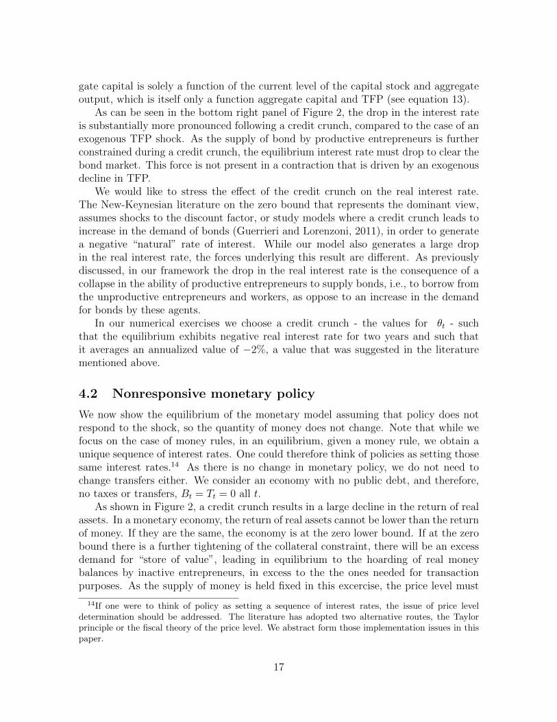
gate capital is solely a function of the current level of the capital stock and aggregateoutput, which is itself only a function aggregate capital and TFP (see equation 13).

As can be seen in the bottom right panel of Figure 2, the drop in the interest rateis substantially more pronounced following a credit crunch, compared to the case of anexogenous TFP shock. As the supply of bond by productive entrepreneurs is furtherconstrained during a credit crunch, the equilibrium interest rate must drop to clear thebond market. This force is not present in a contraction that is driven by an exogenousdecline in TFP.

We would like to stress the effect of the credit crunch on the real interest rate.The New-Keynesian literature on the zero bound that represents the dominant view,assumes shocks to the discount factor, or study models where a credit crunch leads toincrease in the demand of bonds (Guerrieri and Lorenzoni, 2011), in order to generatea negative “natural” rate of interest. While our model also generates a large dropin the real interest rate, the forces underlying this result are different. As previouslydiscussed, in our framework the drop in the real interest rate is the consequence of acollapse in the ability of productive entrepreneurs to supply bonds, i.e., to borrow fromthe unproductive entrepreneurs and workers, as oppose to an increase in the demandfor bonds by these agents.

In our numerical exercises we choose a credit crunch - the values for θt - suchthat the equilibrium exhibits negative real interest rate for two years and such thatit averages an annualized value of −2%, a value that was suggested in the literaturementioned above.

4.2 Nonresponsive monetary policy

We now show the equilibrium of the monetary model assuming that policy does notrespond to the shock, so the quantity of money does not change. Note that while wefocus on the case of money rules, in an equilibrium, given a money rule, we obtain aunique sequence of interest rates. One could therefore think of policies as setting thosesame interest rates.14 As there is no change in monetary policy, we do not need tochange transfers either. We consider an economy with no public debt, and therefore,no taxes or transfers, Bt = Tt = 0 all t.

As shown in Figure 2, a credit crunch results in a large decline in the return of realassets. In a monetary economy, the return of real assets cannot be lower than the returnof money. If they are the same, the economy is at the zero lower bound. If at the zerobound there is a further tightening of the collateral constraint, there will be an excessdemand for “store of value”, leading in equilibrium to the hoarding of real moneybalances by inactive entrepreneurs, in excess to the the ones needed for transactionpurposes. As the supply of money is held fixed in this excercise, the price level must

14If one were to think of policy as setting a sequence of interest rates, the issue of price leveldetermination should be addressed. The literature has adopted two alternative routes, the Taylorprinciple or the fiscal theory of the price level. We abstract form those implementation issues in thispaper.

17

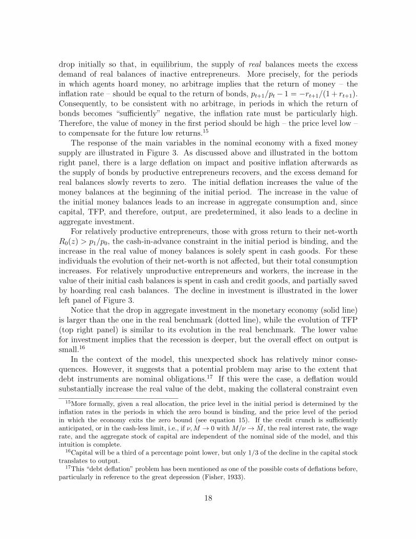
drop initially so that, in equilibrium, the supply of real balances meets the excessdemand of real balances of inactive entrepreneurs. More precisely, for the periodsin which agents hoard money, no arbitrage implies that the return of money – theinflation rate – should be equal to the return of bonds, pt+1/pt− 1 = −rt+1/(1 + rt+1).Consequently, to be consistent with no arbitrage, in periods in which the return ofbonds becomes “sufficiently” negative, the inflation rate must be particularly high.Therefore, the value of money in the first period should be high – the price level low –to compensate for the future low returns.15

The response of the main variables in the nominal economy with a fixed moneysupply are illustrated in Figure 3. As discussed above and illustrated in the bottomright panel, there is a large deflation on impact and positive inflation afterwards asthe supply of bonds by productive entrepreneurs recovers, and the excess demand forreal balances slowly reverts to zero. The initial deflation increases the value of themoney balances at the beginning of the initial period. The increase in the value ofthe initial money balances leads to an increase in aggregate consumption and, sincecapital, TFP, and therefore, output, are predetermined, it also leads to a decline inaggregate investment.

For relatively productive entrepreneurs, those with gross return to their net-worthR0(z) > p1/p0, the cash-in-advance constraint in the initial period is binding, and theincrease in the real value of money balances is solely spent in cash goods. For theseindividuals the evolution of their net-worth is not affected, but their total consumptionincreases. For relatively unproductive entrepreneurs and workers, the increase in thevalue of their initial cash balances is spent in cash and credit goods, and partially savedby hoarding real cash balances. The decline in investment is illustrated in the lowerleft panel of Figure 3.

Notice that the drop in aggregate investment in the monetary economy (solid line)is larger than the one in the real benchmark (dotted line), while the evolution of TFP(top right panel) is similar to its evolution in the real benchmark. The lower valuefor investment implies that the recession is deeper, but the overall effect on output issmall.16

In the context of the model, this unexpected shock has relatively minor conse-quences. However, it suggests that a potential problem may arise to the extent thatdebt instruments are nominal obligations.17 If this were the case, a deflation wouldsubstantially increase the real value of the debt, making the collateral constraint even

15More formally, given a real allocation, the price level in the initial period is determined by theinflation rates in the periods in which the zero bound is binding, and the price level of the periodin which the economy exits the zero bound (see equation 15). If the credit crunch is sufficientlyanticipated, or in the cash-less limit, i.e., if ν,M → 0 with M/ν → M , the real interest rate, the wagerate, and the aggregate stock of capital are independent of the nominal side of the model, and thisintuition is complete.

16Capital will be a third of a percentage point lower, but only 1/3 of the decline in the capital stocktranslates to output.

17This “debt deflation” problem has been mentioned as one of the possible costs of deflations before,particularly in reference to the great depression (Fisher, 1933).

18

0 10 200.94

0.96

0.98

1

output

0 10 200.94

0.96

0.98

1

TFP

0 10 200.94

0.96

0.98

1

capital

quarters

bmk real

real debt

0 10 20

−0.2

−0.1

0

inflation

quarters

Figure 3: Aggregate Implications of a Credit Crunch: Constant Money

tighter.

4.2.1 Nominal Bonds

In order to explore this possibility, we solve the model assuming that entrepreneursonly issue nominal bonds. In particular, we assume that active entrepreneurs financetheir investment by issuing one period nominal bonds. As before, the real value ofbond issuance are restricted by the collateral constraint in (3).

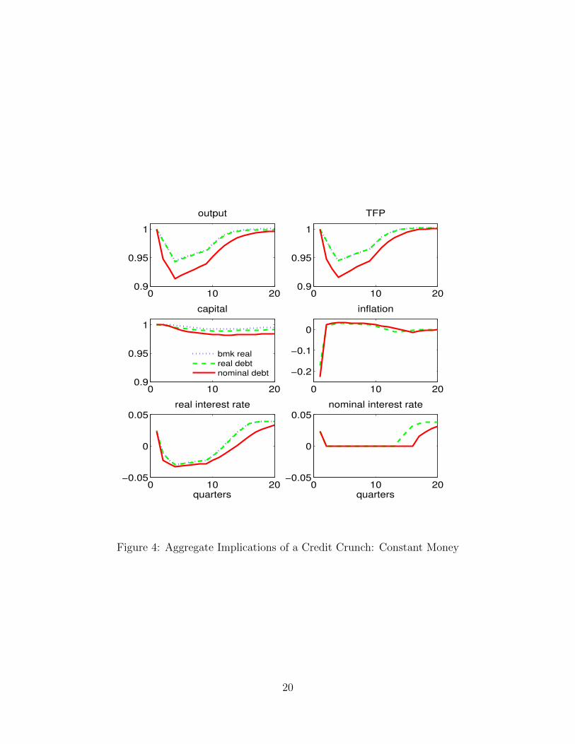
The results, which are dramatically different, are depicted in Figure 4, which alsoplots both the benchmark (dotted line) and the case of indexed debt (dashed line).The recession is deeper and more persistent, driven mainly by a sharper decline inTFP. The intuition for the dramatic effect of the debt deflation is simple: The initialdeflation implies a large redistribution from high productivity, leveraged entrepreneurstowards bondholders, who are inactive, unproductive entrepreneurs. The ability ofproductive entrepreneurs to invest is now hampered by both the tightening of collateralconstraints and the decline of their net-worth. As a consequence, there needs to be alarger decline in the real interest rate so that in equilibrium more capital is reallocatedfrom productive to unproductive entrepreneurs (bottom left panel).

The discussion above suggests that the initial deflation can be very costly in terms

19

0 10 200.9

0.95

1

output

0 10 200.9

0.95

1

TFP

0 10 200.9

0.95

1

capital

0 10 20

−0.2

−0.1

0

inflation

0 10 20−0.05

0

0.05real interest rate

quarters0 10 20

−0.05

0

0.05nominal interest rate

quarters

bmk real

real debt

nominal debt

Figure 4: Aggregate Implications of a Credit Crunch: Constant Money

20

of output, in the case in which debt is a nominal obligation. An obvious question is,then, what can monetary policy do, if anything, to stabilize output. We consider thosecases next.

4.3 Inflation targeting

We now consider the case of a Central Bank whose objective is to implement an infla-tion target of π = pt+1/pt − 1 for all t. In order to implement the inflation target π,the government needs to adjust the supply of assets, i.e., real money balances Mt+1/ptand government bonds Bt+1, and the associated lump-sum tax sequences Tt(z), TWt ,to accommodate changes in the desired demand for real money balances, and more im-portantly, to satisfy the excess demand for assets during a credit crunch. In particular,without loss of generality, we assume that the government sets the quantity of moneyto be equal to the money required by individuals to finance their purchases of cashgood in every period, mT

t+1, given by equation (9),

Mt+1 = ptν(1− β)β

1− ν(1− β)

[∫Rt+1(z)Φt+1(dz)−

∞∑j=0

∫ ∞0

Tt+j (z)∏js=1Rt+s (z)

Ψ(dz)

],

and that the public debt accommodates the excess demand for bonds in periods wherethe real interest rate equals the constants return of money rt+1 = −π/(1 + π),

Bt+1 =

{Bt if rt+1 > − π

1+π∫ zt+1

0Φt+1(dz)− (λt+1 − 1)

∫∞zt+1

Φt+1(dz) if rt+1 = − π1+π

. (16)

Obviously, lump-sum taxes (subsidies) must be adjusted accordingly to satisfy thegovernment budget constraint in (10).

These conditions fully determined the evolution of the money supply, governmentbonds, and the aggregate level of taxes (transfers), but they leave unspecified how taxes(transfers) are distributed across entrepreneurs and workers. We consider two simplecases: First, we present results for the case that taxes (transfers) are purely lump-sum,i.e., Tt(z) = TWt = Tt for all t, z.18 We refer to this as the “lump-sum” case. Thesecond case that we consider is one where taxes (transfers) are purely lump-sum forall period with the exception of those when the government expands the supply ofgovernment bonds, i.e., Bt+1 > Bt. In the periods when the government increasesthe supply of bonds, we assume that the proceeds from the sell bonds, net of interestpayments, and the adjustment of the supply of real balances are only rebated to the

18In this section we need to specify the relative number of workers and entrepreneurs in the economy.We assume that workers are 25% of the population, L/(1 + L) = 1/4. We choose a low share ofworkers, who in our model choose to be against their borrowing constraint in a steady state, to limitthe non-Ricardian elements in the model.

21

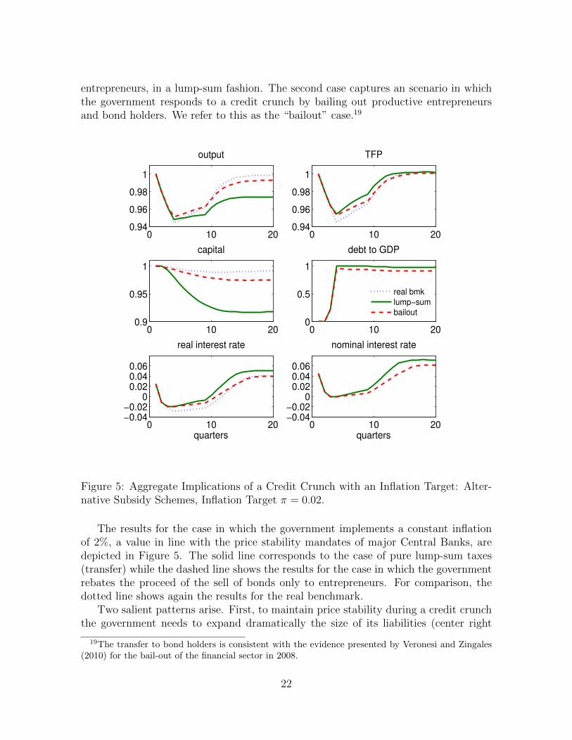
entrepreneurs, in a lump-sum fashion. The second case captures an scenario in whichthe government responds to a credit crunch by bailing out productive entrepreneursand bond holders. We refer to this as the “bailout” case.19

0 10 200.94

0.96

0.98

1

output

0 10 200.94

0.96

0.98

1

TFP

0 10 200.9

0.95

1

capital

0 10 200

0.5

1

debt to GDP

real bmk

lump−sum

bailout

0 10 20−0.04−0.02

00.020.040.06

real interest rate

quarters0 10 20

−0.04−0.02

00.020.040.06

nominal interest rate

quarters

Figure 5: Aggregate Implications of a Credit Crunch with an Inflation Target: Alter-native Subsidy Schemes, Inflation Target π = 0.02.

The results for the case in which the government implements a constant inflationof 2%, a value in line with the price stability mandates of major Central Banks, aredepicted in Figure 5. The solid line corresponds to the case of pure lump-sum taxes(transfer) while the dashed line shows the results for the case in which the governmentrebates the proceed of the sell of bonds only to entrepreneurs. For comparison, thedotted line shows again the results for the real benchmark.

Two salient patterns arise. First, to maintain price stability during a credit crunchthe government needs to expand dramatically the size of its liabilities (center right

19The transfer to bond holders is consistent with the evidence presented by Veronesi and Zingales(2010) for the bail-out of the financial sector in 2008.

22

panel). Second, when implementing a low inflation, and therefore, constraining thereal interest rate to be higher, the government attains a less pronounce recession atthe cost of a slower recovery.

In a credit crunch the capacity of productive entrepreneurs to supply bonds isreduced, resulting in an excess demand of saving instruments by unproductive en-trepreneurs and workers.20 To avoid the deflation induced by the excess demand ofmediums to “store of value”, the government must increase the supply of governmentbonds or money, which at the zero bound are perfect substitute. Furthermore, theincrease in the supply of government bonds induces a further increase in the demandof these bonds by unconstrained entrepreneurs, as these agents save in anticipation ofthe higher taxes that will be raised to pay the interest of this debt.

As the top left panel of Figure 5 shows, with this policy the government accom-plishes a slightly less pronounced recession at the cost of significantly more protractedrecovery. The milder recession is explained by the smaller drop in TFP. When the gov-ernment maintains the inflation low, the real interest rate is constrained to be higher,and therefore, there is less reallocation of capital toward less productive, and previouslyinactive, entrepreneurs. The counterpart of the milder drop in TFP is a collapse ininvestment, leading to a substantial and persistence decline in the stock of capital.

In our framework Ricardian equivalence does not hold, and increases in governmentdebt crowds out private investment. This is particularly true for the case in which thegovernment uses pure lump-sum taxes (solid line). In this case, part of the transfersgo to workers, who in equilibrium have a large marginal propensity to consume as theywill be against their borrowing constraint in finite time.21 Thus, when the governmentincreases the supply of bonds, and transfers the proceeds of the sell of these bonds tohouseholds, aggregate consumptions increases, and investment decreases, relative tothe real benchmark economy.

In comparison, the recovery is faster when the government rebates the proceedsfrom the increase in the debt solely to entrepreneurs (dashed line). Nevertheless, thedrop in investment is still more pronounced that in the real benchmark. There aretwo reasons why Ricardian equivalence does not hold in this case. Firstly, productiveentrepreneurs choose to consume part of the higher government transfers. Productiveentrepreneurs discount future taxes at a rate that is higher than the interest rate,i.e., for infra-marginal entrepreneurs, z > zt+1, Rt+1(z) > (1 + rt+1). Secondly, eveninactive entrepreneurs, who discount the future at the same rate as the government,face initially a sequence of transfers and taxes that have a strictly positive net presentvalue. This is because in this case entrepreneurs receive a disproportionally large shareof transfers, while taxes are uniformly distributed among entrepreneurs and workers.

20In the real benchmark, at the beginning of the credit crunch workers accumulate assets as thecredit crunch it anticipated one period in advance, and the lowest value of the collateral constraintconstraint is attained in the forth quarter.

21In a steady state the interest rate is strictly lower than the rate of time preferences, (1+r∞)β < 1.Therefore, workers, who earn a flow of labor income each period, will choose to be against theirborrowing constraint in finite time.

23

0 10 200.94

0.96

0.98

1

output

0 10 200.94

0.96

0.98

1

TFP

0 10 200.9

0.95

1

capital

π=0.03

π=0.00

0 10 200

2

4

debt to GDP

π=0.01

π=0.02

0 10 20−0.04−0.02

00.020.040.06

real interest rate

quarters0 10 20

−0.04−0.02

00.020.040.06

nominal interest rate

quarters

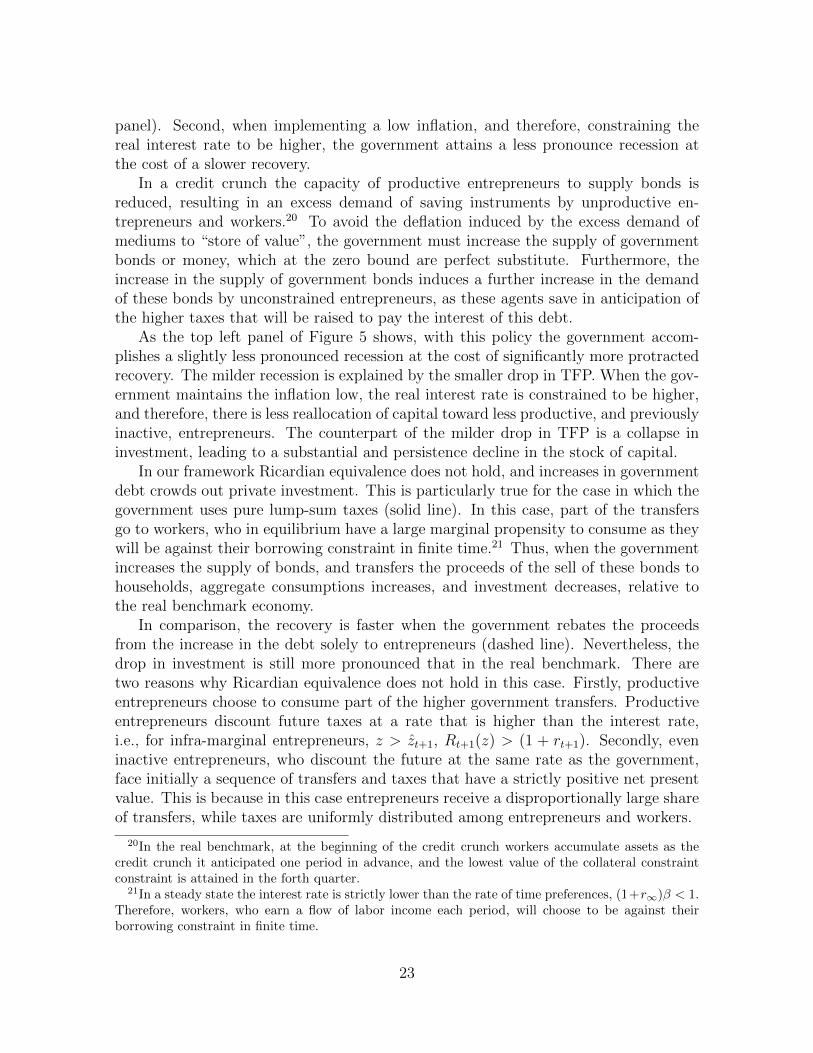
Figure 6: Aggregate Implication of a Credit Crunch with an Inflation Target: Alter-native Inflation Targets, Bailout Case.

Can the government mitigate the consequences of a credit crunch by choosing al-ternative inflation targets? In particular, is it desirable that the government choosesa sufficiently high inflation target in order to avoid the zero lower bound? We explorethis question in Figure 6. There we present the evolution of four economies differingin the level of the inflation target, π = 0, 0.01, 0.02, and 0.03. In all these cases weassume that the government rebates the proceeds from the increase in the debt solelyto entrepreneurs (bailout case).

The two main features of the previous examples are reinforced for the economieswith a lower inflation target. The lower the inflation target is, the less pronounced therecession in the short run is. At the same time, the recovery is slower. furthermore,the government will need a larger increase in the supply of bonds to implement a lowerinflation target. The larger increase in the government debt will imply a larger crowd-out of investment. On the contrary, for a sufficiently large inflation target, π = 0.03 in

24

our example, the government reproduces closely the equilibrium in the real benchmarkeconomy. The dynamics of the nominal interest rate is common across these examples.The nominal interest rate are at zero, or close to zero, for various quarters.

The case of a government implementing a low inflation seems attractive to interpretthe Great Recession in the US. Following the 2008 crisis, the economy has been forseveral quarters at the zero bound, while the Fed has increased substantially its balancesheet. The Fed policy has been directed explicitly to provide the US economy withsafe zero nominal interest rate money-like-assets, while inflation has been under totalcontrol. All these features are reproduced by this example. Moreover, there is apresumption that these policies avoided a more severe recession, although the recoveryis seen as unusually slow. Again, a feature of the aggregate economy in this example.

5 Distribution of Welfare Impacts

In the previous section we focused on the impact of policies on aggregate outcomesand factor prices. The aggregate figures suggest a relatively simple trade-off at theaggregate level. These dynamics, though, hide very disparate effects of a credit crunch,and alternative monetary policies, among different agents. While workers are hurt bythe drop in wages, the profitability of active entrepreneurs, and their welfare, increasesas a result of lower factor prices. Similarly, unproductive entrepreneurs are bondholdersin equilibrium, and therefore, are hurt by a decline in the real interest rate.

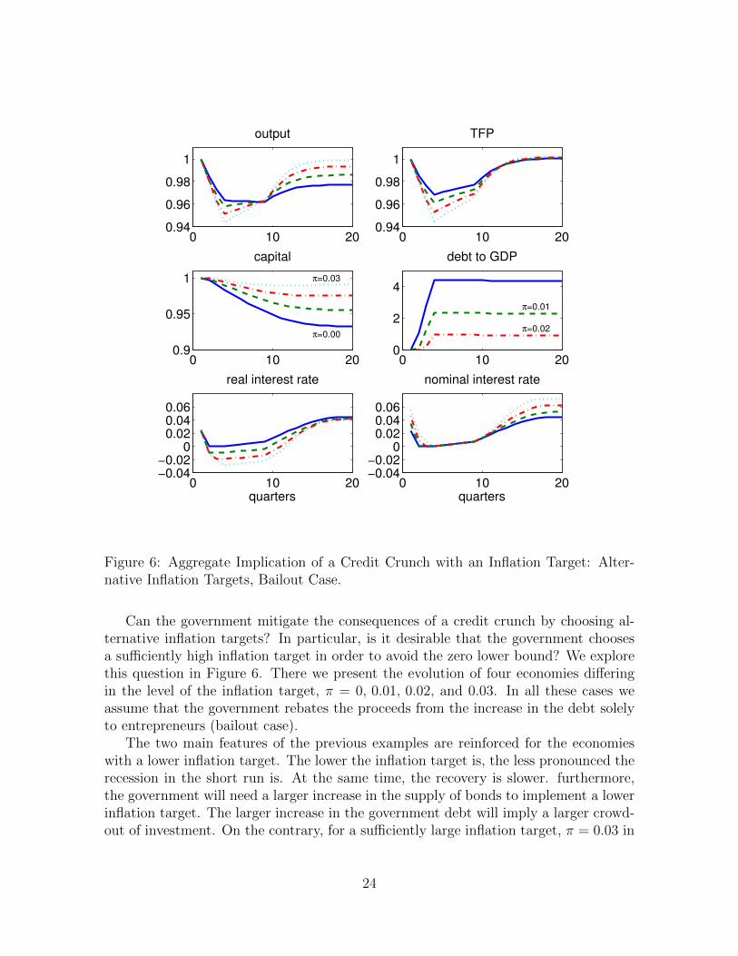
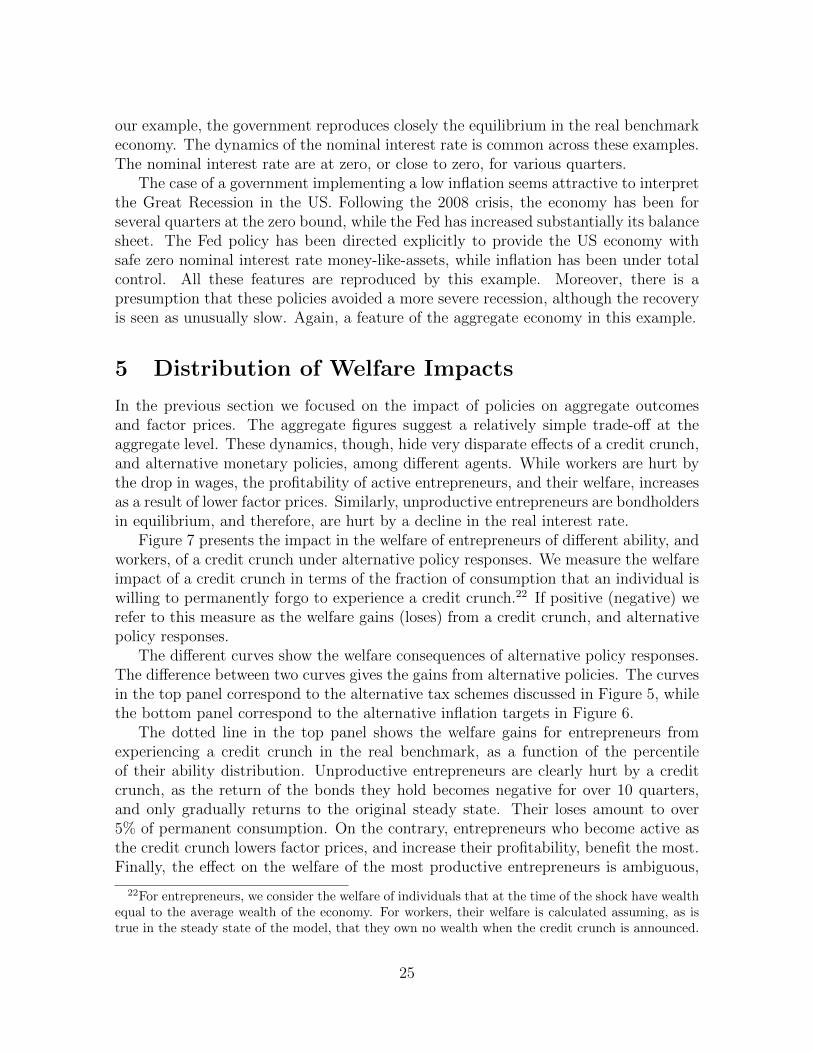
Figure 7 presents the impact in the welfare of entrepreneurs of different ability, andworkers, of a credit crunch under alternative policy responses. We measure the welfareimpact of a credit crunch in terms of the fraction of consumption that an individual iswilling to permanently forgo to experience a credit crunch.22 If positive (negative) werefer to this measure as the welfare gains (loses) from a credit crunch, and alternativepolicy responses.

The different curves show the welfare consequences of alternative policy responses.The difference between two curves gives the gains from alternative policies. The curvesin the top panel correspond to the alternative tax schemes discussed in Figure 5, whilethe bottom panel correspond to the alternative inflation targets in Figure 6.

The dotted line in the top panel shows the welfare gains for entrepreneurs fromexperiencing a credit crunch in the real benchmark, as a function of the percentileof their ability distribution. Unproductive entrepreneurs are clearly hurt by a creditcrunch, as the return of the bonds they hold becomes negative for over 10 quarters,and only gradually returns to the original steady state. Their loses amount to over5% of permanent consumption. On the contrary, entrepreneurs who become active asthe credit crunch lowers factor prices, and increase their profitability, benefit the most.Finally, the effect on the welfare of the most productive entrepreneurs is ambiguous,

22For entrepreneurs, we consider the welfare of individuals that at the time of the shock have wealthequal to the average wealth of the economy. For workers, their welfare is calculated assuming, as istrue in the steady state of the model, that they own no wealth when the credit crunch is announced.

25

0.8 0.82 0.84 0.86 0.88 0.9 0.92 0.94 0.96 0.98 1

0

0.2

0.4

0.6

fraction o

f consum

ption

Alternative Taxes and Subsidies, π=0.02

real bmk, wgW

= −0.006

lump−sum, wgW

= −0.013

bailout, wgW

= −0.02

0.8 0.82 0.84 0.86 0.88 0.9 0.92 0.94 0.96 0.98 1

0

0.2

0.4

ability percentile

fraction o

f consum

ption

Alternative Inflation Targets, Bailout Case

π = 0.01, wgW

= −0.044

π = 0.02, wgW

= −0.02

π = 0.03, wgW

= −0.0049

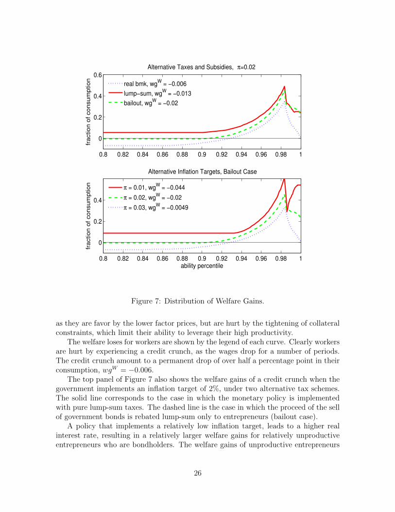
Figure 7: Distribution of Welfare Gains.

as they are favor by the lower factor prices, but are hurt by the tightening of collateralconstraints, which limit their ability to leverage their high productivity.

The welfare loses for workers are shown by the legend of each curve. Clearly workersare hurt by experiencing a credit crunch, as the wages drop for a number of periods.The credit crunch amount to a permanent drop of over half a percentage point in theirconsumption, wgW = −0.006.

The top panel of Figure 7 also shows the welfare gains of a credit crunch when thegovernment implements an inflation target of 2%, under two alternative tax schemes.The solid line corresponds to the case in which the monetary policy is implementedwith pure lump-sum taxes. The dashed line is the case in which the proceed of the sellof government bonds is rebated lump-sum only to entrepreneurs (bailout case).

A policy that implements a relatively low inflation target, leads to a higher realinterest rate, resulting in a relatively larger welfare gains for relatively unproductiveentrepreneurs who are bondholders. The welfare gains of unproductive entrepreneurs

26

are at expense of workers, who do not hold bonds in the steady state, but end up payinghigher taxes to finance the interest payment of the government debt. Intuitively, thewelfare loses of workers are highest when the proceed of the sell of bonds is rebatedsolely to entrepreneurs, wgW = 0.02, compare to the pure lump-sum case, wgW =0.0013.

The bottom panel shows the welfare consequences of alternative inflation targets,for the case in which the government rebates the proceed of the sell of bonds solely toentrepreneurs. The lowest the inflation target the highest the real interest rate, bothduring the credit crunch, and in the new steady state.23 Unproductive entrepreneursbenefit from the highest interest rate. Similarly, productive entrepreneurs benefit fromthe lowest wages associated with the lowest capital during the transition, and in thenew steady state. Although individual entrepreneurs do not internalize it, collectivelythey benefit from the lower wages associated with a lower aggregate stock of capital.

6 Conclusions

TO BE WRITTEN.

7 Appendix

TO BE WRITTEN.

23Given the debt policy equation (16), the government debt in the new steady state will be highestthe lowest the inflation target is. In the model, a higher level of government debt implies a lower levelof capital in the new steady state.

27

References

Buera, F. J. and B. Moll (2012): “Aggregate Implications of a Credit Crunch,”

NBER Working Papers 17775, National Bureau of Economic Research, Inc.

Christiano, L., M. Eichenbaum, and S. Rebelo (2011): “When Is the Govern-

ment Spending Multiplier Large?” Journal of Political Economy, 119, 78 – 121.

Correia, I., E. Farhi, J. P. Nicolini, and P. Teles (forthcoming): “Unconven-

tional Fiscal Policy at the Zero Bound,” American Economic Review.

Curdia, V. and G. Eggertsson (2009): “What Caused the Great Depression?”

Manuscript, Federal Reserve Bank of New York.

Diaz-Alejandro, C. (1985): “Good-bye financial repression, hello financial crash,”

Journal of Development Economics, 19, 1–24.

Drautzburg, T. and H. Uhlig (2011): “Fiscal Stimulus and Distortionary Taxa-

tion,” NBER Working Papers 17111, National Bureau of Economic Research, Inc.

Eggertsson, G. B. (2011): “What Fiscal Policy is Effective at Zero Interest Rates?”

in NBER Macroeconomics Annual 2010, Volume 25, National Bureau of Economic

Research, Inc, NBER Chapters, 59–112.

Eggertsson, G. B. and M. Woodford (2003): “The Zero Bound on Interest

Rates and Optimal Monetary Policy,” Brookings Papers on Economic Activity, 34,

139–235.

Fisher, I. (1933): “The Debt-Deflation Theory of Great Depressions,” Econometrica,

1, 337–357.

Friedman, M. and A. Schwartz (1963): A Monetary History of the United States,

1867-1960, Princeton University Press.

Galı, J., F. Smets, and R. Wouters (2011): “Unemployment in an Estimated

New Keynesian Model,” NBER Working Papers 17084, National Bureau of Economic

Research, Inc.

Guerrieri, V. and G. Lorenzoni (2011): “Credit Crises, Precautionary Savings,

and the Liquidity Trap,” NBER Working Papers 17583, National Bureau of Eco-

nomic Research, Inc.

28

Krugman, P. R. (1998): “It’s Baaack: Japan’s Slump and the Return of the Liquidity

Trap,” Brookings Papers on Economic Activity, 29, 137–206.

Lucas, R. E. and J. P. Nicolini (2013): “On the Stability of Money Demand,”

Manuscript, Federal Reserve Bank of Minneapolis.

Moll, B. (2012): “Productivity Losses from Financial Frictions: Can Self-financing

Undo Capital Misallocation?” Manuscript, Princeton University.

Svensson, L. E. O. (1985): “Money and Asset Prices in a Cash-in-Advance Econ-

omy,” Journal of Political Economy, 93, 919–44.

Veronesi, P. and L. Zingales (2010): “Paulson’s gift,” Journal of Financial Eco-

nomics, 97, 339–368.

Werning, I. (2011): “Managing a Liquidity Trap: Monetary and Fiscal Policy,”

NBER Working Papers 17344, National Bureau of Economic Research, Inc.

29