Liquidity in the U - New York Universitypeople.stern.nyu.edu/jhasbrou/Research/Working Papers...Page...

Liquidity in the Futures Pits: Inferring Market Dynamics from Incomplete Data

Joel Hasbrouck

This Draft: March 18, 2003

Comments Welcome

Kenneth M. Langone Professor of Finance Stern School of Business New York University Suite 9-190 Mail Code 0268 44 West Fourth St. New York, NY 10012-1126

Tel: (212) 998-0310 Fax: (212) 995–4901 E-mail: [email protected] Web: http://www.stern.nyu.edu/~jhasbrou

For comments on an earlier draft, I am grateful to Larry Harris, Ken Kavajecz, Peter Locke, Nick Polson, the Chicago Mercantile Exchange, and seminar participants at Duke University, the University of Chicago, Vanderbilt University, Wharton and the Western Finance Association. I am grateful for financial support from a Stern Summer Research Grant. An appendix that describes the computational details of this paper, and all programs and data are available on my web site. All errors are my own responsibility.

http://www.stern.nyu.edu/~jhasbrou

Liquidity in the Futures Pits: Inferring Market Dynamics from Incomplete Data

Abstract

Motivated by economic models of sequential trade, empirical analyses of market

dynamics frequently estimate liquidity as the coefficient of signed order flow in a price-

change regression. This paper implements such an analysis for futures transaction data

from pit trading. To deal with the absence of timely bid and ask quotes (which are used to

sign trades in most equity-market studies), this paper proposes new techniques based on

Markov chain Monte Carlo estimation.

The model is estimated for four representative Chicago Mercantile Exchange

contracts. The highest liquidity (lowest order flow coefficient) is found for the S&P

index. Liquidity for the Euro and UK £ contracts is somewhat lower. The pork belly

contract exhibits the least liquidity.

Keywords: Futures Markets, Liquidity, Gibbs Sampler, MCMC,

Markov chain Monte Carlo, Foreign Exchange, Stock Index Futures.

JEL Classification: C1, C11, C13, C15, G1, G10

1. Introduction

US futures exchanges utilize a physically convened open outcry trading

mechanism that poses particular challenges to the measurement of trading costs, order

impacts and other attributes of liquidity. The present perspective, based on sequential

trade models of asymmetric information, is very similar to the approach widely used in

equity studies. Specifically, quote setters post bid and/or offer quotes, potential traders

arrive and buy or sell, and after any trade, quotes are revised. This logic supports

dynamic models in which price changes are regressed against order flows that are signed

(positively for buyer-initiated and negatively for seller-initiated orders). 1

These specifications, however, make strong demands on market data.

Construction of signed order flow generally requires data for both transactions (price and

volume) and quotes (bid and ask). While quote data are commonly available for equity

markets, and markets that are organized as electronic limit order books, they are not

generally available for open outcry markets. Specifically, bids and offers in futures pits

expire (unless hit) virtually instantaneously, and are therefore seldom recorded.

The analysis of futures trading in the present paper is based on a novel

econometric approach that facilitates estimation of rich microstructure models from

limited data. In this approach, the bid, ask and, most importantly, the direction (sign) of a

given trade are viewed as latent, unobserved variables. I sign a trade, or, (more

accurately) derive a probability density for the sign of the trade, conditional on the model

and all observed data.

This is essentially the modeling perspective of Glosten and Harris (1988). The

present analysis generalizes their model in numerous respects, and suggests a new

direction in estimation approach. Glosten and Harris use a non-linear state-space,

1 Theoretical analyses include Glosten and Milgrom (1985), Easley and O'Hara (1992a); Easley and O'Hara (1991); Easley and O'Hara (1987); Easley and O'Hara (1992b) and O'Hara (1995). Representative empirical studies include Hasbrouck (1991a); Hasbrouck (1996a); Huang and Stoll (1994); Huang and Stoll (1997) and Madhavan, Richardson, and Roomans (1997).

maximum likelihood approach. This paper implements a Bayesian analysis using a

Markov chain Monte Carlo (MCMC) estimator, the Gibbs sampler, which is attractive

both analytically and computationally.2 Bayesian methods are usually employed to

incorporate prior beliefs about parameters. The more compelling motivation for the use

of Bayesian methods in the present case, however, lies in the analytical and

computational ease with which latent variables (such as the unobserved trade direction)

may be incorporated.

The paper presents analyses for the CME pork belly, Euro, UK £ and S&P 500

index contracts, for two microstructure specifications. The first is a variant of the Roll

(1984) model. This is a useful starting point due to its simplicity and the availability of an

alternative estimation technique, the (standard) moment approach. The second

specification allows for price discreteness, clustering and trade-price impacts. The

estimates of this model for the four contracts suggest substantial (and presumably

informational) effects of trades on prices, non-informational costs of market-making that

are small relative to the tick size, and (for the pork-belly and S&P contracts) significant

price clustering. Taking the price impact coefficient as a summary measure of liquidity,

the S&P contract is the most liquid, followed by the two currency contracts, and the pork

belly contract is the least liquid.

Excellent prior studies of futures market liquidity are available. Those based on

transaction-level data include Laux and Senchack (1992) and Ma, Peterson, and Sears

(1992). These analyses employ moment-based estimates of the Roll model. For the

present data, moment estimates are significantly higher than the corresponding MCMC

estimates. The Roll model does not allow for informational price impacts. Manaster and

2 Bayesian MCMC applications in market microstructure include Hasbrouck (1999b) and Ball and Chordia (2001). The techniques have also been used extensively in the analysis of stochastic volatility models (Shephard (1993); Engle (1994); Jacquier, Polson, and Rossi (1994); Kim, Shephard, and Chib (1998); Jones (2002)). For textbook expositions, see Carlin and Louis (1996), Gamerman (1997), and Kim and Nelson (2000). Other useful introductory materials include: Gilks, Richardson, and Spiegelhalter (1996) (for a concise overview of MCMC techniques), Casella and George (1992) (for the Gibbs sampler) and Chib and Greenberg (1996) (for applications in econometrics).

Mann (1996) and Locke and Venkatesh (1997) use Computerized Trade Reconstruction

(CTR) data. These data (which are not publicly available) establish trader identity, permit

tracking of trader positions, and so support a range of interesting analyses concerning

inventory control. Manaster and Mann also estimate order impacts contingent on class of

trader. Identification of a buyer and seller does not, however, establish who initiated the

trade (in the sense of the sequential trade models), i.e., which party hit or lifted the bid or

ask exposed by the other.

The paper is organized as follows. The next section summarizes trading

procedures and some key features of the futures data. The paper then treats a simple and

familiar microstructure construct (the Roll (1984) model of the bid-ask spread) from both

conventional and modern Bayesian approaches (Section 3). A more comprehensive and

realistic model that incorporates asymmetric information, discreteness and clustering is

presented in Section 4. Section 5 covers results for the futures contracts. Section 6

discusses extensions. A brief summary concludes the paper in Section 7.

2. Institutional background and preliminary features of the data

The Chicago Mercantile Exchange is a major U.S. futures exchange. Their web

site (at www.cme.com) provides a comprehensive description of the Exchange,

instruments, trading mechanisms and data (including that used in the present study). The

trading arrangements at the CME are typical of U.S. futures exchanges. Traders interact

face-to-face on the exchange floor. They compete by shouting and signing acceptable

price/trade combinations. There is no presumption that a bid or offer is good until

explicitly canceled or modified. A trader who wishes to signal ongoing availability of a

price may continually repeat a bid or offer. This transience does not, however, invalidate

the sequential trade framework, since we are still in a world where the quote setter moves

first and the (potential) “market order” trader follows.

An observer on the floor sees bids, offers and trades. In real time, however, off-

floor participants must rely on the electronically disseminated tick data. The reported

price is the most current trade price. This is updated only when a trade at a new price

occurs. This differs from the last sale reporting practices in U.S. equities markets,

wherein a trade is reported even if it is at the same price as the previous trade. Smith and

Whaley (1994) discuss estimators of the Roll bid-ask spread using time and sales data.

The data used in the present study are drawn from the CME’s volume-tick files,

and consist of time-stamped trade prices and volumes. These data encompass all trades

(not just those with nonzero price changes), and thus constitute a record substantially

similar to what researchers employ from the U.S. equity market’s Consolidated

Transaction System. The sample consists of trading data for one month for four

representative contracts. The contracts are: pork bellies (an important agricultural

commodity); the Euro (the dominant currency contract); the UK £ (an actively traded

non-EMU currency); and the S&P 500 index (the dominant stock index contract).

These data are synthesized from tick reports, clearing records and audit

information. They are essentially the computerized trade reconstruction (CTR) data used

by Manaster and Mann (1996), Ferguson, Mann, and Schneck (1998) and others, with

trader identifications suppressed. Because the CTR data are constructed from clearing

records, there are not likely to be many spurious or omitted trades. The time stamps

assigned to the trades, however, are less certain. The empirical specifications used here

derive from the sequential trade models. For present purposes, therefore, errors in time

stamps are most serious when they reorder the trades. This concern cannot be summarily

dismissed. Current reporting practices, however, are considerably improved over earlier

procedures.3 Indeterminate time assignments in CTR data generally appear as clustering

in the time reports of trades with the CME’s fifteen-minute reporting windows. The time

reports in this sample are indeed clustered at one- and fifteen-minute intervals. Although

discernible, however, the clustering is not highly pronounced. This suggests that time

stamps are not being systematically shifted in a large and obvious way.

3 The trade time is generally the time stamp of execution in the pit. This is bracketed by two other time stamps entered by the broker’s clerk: a stamp when the order was received from the customer and another when the execution report was received.

Table 1

Table 1

describes various features of the analyzed contracts. Of particular

relevance for the paper are the tick sizes. As a proportion of the contract price, they are

often dramatically lower than those commonly encountered in equity markets. A tick of

$1/16 is 0.125% of a $50 stock. This is somewhat greater than that of any of the futures

contracts. The standard deviation of the price change measured in ticks, however, is

relatively small. This suggests that the tick size is not negligible relative to phenomena of

economic interest, and furthermore suggests the importance of modeling discreteness.

also describes the scale and timing of the transactions. For sheer pace of

trading activity, the S&P composite contract stands out. It exhibits an average

intertransaction time of only five seconds. Trades frequently occurred within the same

second. The economic framework of the sequential trade models generally assumes that

trade reports are instantaneously disseminated and evaluated. In the S&P index pit, at

least, an individual trader’s information set is unlikely to be this current.

This preliminary analysis suggests the following considerations for modeling

strategy. First, motivated by the economic sequential trade models, it seems desirable (as

in the equity market studies) to allow for trade-driven price impacts of both a transient

(cost-related) and permanent (informational) nature. The results of this section suggest

that in addition, discreteness is important because the tick size is generally on the same

scale as intertransaction volatility.

3. The Bayesian approach to estimation of microstructure models

This section discusses the essentials of modern Bayesian estimation in the context

of market microstructure analyses. By virtue of its simplicity and familiarity, the Roll

(1984) model of the bid-ask spread is a convenient starting point. The discussion presents

the model, classical and Bayesian approaches to estimation, and the application to the

futures market data.

a. The basic Roll model

A variant of the Roll model is as follows. Let the efficient price be denoted Mt. Its

logarithm is assumed to evolve as a normal random walk: (logtm = )tM

( )21 where the are i.i.d. 0,t t t t um m u u N σ−= + . (1)

The term “efficient price” is used here in the sense common to the sequential trade

models, i.e., the expected terminal value of the security conditional on all public

information (including the trade history). The ut reflect new public information. The (log)

bid and ask prices are given as

t t

t t

b m ca m c= −= +

(2)

where c is the nonnegative half-spread. In this framework, c is the execution cost paid by

the active buyer or seller, presently reported by equity markets in conformance with SEC

rule 11ac1-5 (U.S. Securities and Exchange Commission (2001)). Under additional

assumptions (absence of asymmetric information, fixed trading costs, competition among

dealers, etc.), c will be equal to the cost of market making, but this interpretation is not

necessary to motivate the model.

The direction of the incoming order is given by the Bernoulli random

variable { }1, 1tq ∈ − + , where –1 indicates an order to sell (to the quote-setter) and +1

indicates an order to buy (from the quote-setter). Buys and sells are assumed equally

probable. In the standard implementation, qt is assumed independent of , i.e.,

that the direction of the trade is independent of the efficient price movement. This

assumption is restrictive because it rules out the asymmetric information aspects of the

sequential trade models. It is relaxed in later sections. Depending on qt, the (log)

transaction price is either at the bid or the ask:

tm u∆ = t

if 1if 1

t tt

t t

b qp

a q= −

= = + (3)

The model parameters are c and uσ . Inference is based on a time series sample of

trade prices { }1 2, , , Tp p p p= … . The following sections describe method-of-moments

classical and Bayesian approaches to estimation. In the present application, both

approaches assume that the dynamic model given in this section is the correct one.

Although both approaches can accommodate model uncertainty, the present treatment

does not develop this aspect of the problem.

b. The conventional (method of moments) approach

The model implies

( )1 1t t t t t t tp m c q m c q c q u− −∆ = + − + = ∆ + , (4)

from which it follows that:

( )( )

2 2

21

2,

t u

t t

Var p cCov p p c

σ

−

∆ = +∆ ∆ = −

(5)

The corresponding sample estimates for the variance and autocovariance imply estimates

for σu and c that possess all the usual properties of GMM estimators, including

consistency and asymptotic normality. Moment estimation for this model is relatively

easy to implement and often satisfactory.

c. Bayesian estimation

The Bayesian perspective departs most fundamentally from classical approaches

in that parameters are viewed as random variables. This randomness reflects the

statistician’s uncertainty, however, and most emphatically does not imply that parameters

are stochastic within a data sample. Thus in the present model neither c nor σu is time-

varying. The prior distributions impound the initial parameter uncertainty. Estimation

involves construction of parameter posteriors, which are conditional on the observed data

and incorporate all of the information in the observations

Bayesian analyses are often motivated as a means for incorporating prior beliefs,

and are often criticized for sensitivity to choice of prior distributions. In the present

applications, neither of these points is a major consideration. The parameter priors are

essentially uninformative; the posteriors are essentially “data dominated”.4

4 In one interesting respect the parameter prior is substantive, however. Economic logic dictates . The statistical structure of the model actually forces the first-order autocovariance in equation (5) to be nonpositive irrespective of the sign of c. In sample data, however, this property is sometimes violated. In his examination of U.S. stock data, for example, Roll finds that autocovariance estimates based on 21 daily returns are positive roughly half the time. Harris (1990b) notes that positive sample autocovariances will often arise even if the model is correctly specified. Our conviction that is a prior belief, and as such is most naturally incorporated in a Bayesian framework.

0c ≥

0c ≥

The more important motivation for a Bayesian approach here derives from the

power of modern Bayesian techniques for accommodating latent (unobserved) data.

Latent data in the Roll model include bids, asks and trade direction indicators. These

quantities are not artificial features of a statistical model, but are instead constructs that

are economically and structurally meaningful. These latent data are suppressed in the

GMM estimation. GMM procedures are also limited by the difficulty of computing

moments in richer and more realistic models.

The Roll model has two parameters (c and σu) and T latent data values:

{ }1 2, , , Tq q q q= … . The full posterior over parameters and latent data is summarized by

the distribution function ( , ,uF c q pσ ) . There is here (and generally) no tractable closed-

form representation for this function. Instead, it is characterized by simulation, using

techniques that do not require a closed-form representation.

Most of the simulations used in the present paper are Gibbs samplers. The Gibbs

sampler is an iterative procedure. An iteration is generally termed a “sweep”. Initially,

i.e., notationally at the end of sweep 0j = , the parameters and latent data are set to any

values (subject only to feasibility). Denote these initial values { }(0) (0) (0), ,uc qσ . The steps

in the first sweep ( are: )p

1j =

1. Draw ( )(1) (0) (0) from | , ,uc f c qσ

2. Draw ( )(1) (1) (0) from , ,u uf c q pσ σ

3. Draw ( )(1) (1) (1) from , ,uq f q c σ p

Note that all draws are from “full conditional distributions”. That is, all parameters and

latent data except for the component being drawn are taken as given. The next iteration

starts with a draw of ( ) ( ) ( )2 1 conditional on , and uc σ 1q p . Repeating this n times, we

generate a sequence of draws { }2,, ,j j juc qσ for j=1,. . .,n. The Gibbs principle ensures

that the limiting distribution of the nth draw ( )as n →∞ is ( ), ,uF c q pσ , the desired

posterior. From an estimation perspective, the limiting draw for any parameter is

distributed in accordance with the corresponding marginal posterior. For example, the

limiting density of c(n) is ( )|f c p .

How large must n be? The Gibbs sampler is essentially a Markov chain, and the

desired distribution is its limiting distribution. Intuitively, n must be sufficiently large that

dependence on the initial conditions (the starting values) becomes vanishingly small.

Furthermore, the cyclic nature of the Gibbs sampler generally means that successive

draws are dependent. Fortunately, inference does not generally require independent

draws. The c draws, for example, may be viewed as dependent draws from the

parameter posterior. Population parameters of the posterior may be estimated using the

methods of standard time series analysis. For example, the sample mean of the c is a

consistent estimate of

( )j

( )j

[ ]|E c p ; the sample variance is a consistent estimate of [ ]|c pVar ,

and so on.5

The number of draws is limited by computational resources, not sample size.

Furthermore, the limiting distribution (as the number of draws increases) is the exact

small-sample posterior for the given data sample. Finally, suppose that we are interested

in some continuous function of the model parameters, ( ), ug c σ . For a set of parameter

draws, { }( ) ( ), : 1, ,j juc jσ = … n , the corresponding sequence ( ){ }( ) ( ), : 1, ,j j

u j nσ = …g c

generally has as its limiting distribution the posterior for ( )u,g c σ . Transformations of

model parameters are often used in this paper to facilitate presentation and discussion of

results.

The power of Bayesian analysis using the Gibbs sampler derives from the fact

that the full conditional distributions are often tractable. In the present case, for example,

conditional on q, eq. (4) can be treated as a simple regression specification in which c and

σu are the coefficient and residual dispersion, respectively. The normal linear regression

model is a standard Bayesian estimation problem, and it is common practice to use a

5 Of course, determination of the precision of these estimates must take into account the observational dependencies. The standard error of the mean estimate, for example, can be computed using that standard spectral correction described in Hamilton (1994).

normal prior for the coefficients and an inverted gamma prior for the residual dispersion.6

For q, the model suggests obvious priors, specifically 1tq = ± with equal probability.

d. Application to the futures market data

The model discussed above was estimated for the four representative CME

contracts using 10,000 draws of the Gibbs sampler. The computational details of the

draws are described in the appendix to this paper.

The model parameters are c and σu. To expedite the discussion, the exhibits

summarize c, σu and a level version of the cost parameter C c P≡ × , where P is the

average price level (in ticks). Figure 1 depicts histograms of the parameter draws, which

represent (in the limit) the parameter posteriors. These are visually well-defined,

unimodal and concentrated. Table 2 reports summary statistics (labeled “Bayes, q

simulated”).

To place the estimates in perspective, note that we can impute an approximate

annualized volatility for the contracts as ( ) ( )250 .u trading days Avg daily tradesσ × × .

This is an intraday estimate; it excludes overnight price changes. The pork belly contract

averaged 194 trades (Table 1), implying an annualized value of 45%. Values for the

Euro, UK £ and S&P are 6%, 5% and 27%. The C estimates are uniformly less than the

tick size, which motivates a more thorough modeling of discreteness.

By way of comparison, Table 2 also reports conventional moment estimates of the

model. For the volatility parameter, the Bayesian and moment estimates are fairly close

(with the exception of the S&P contract. In the case of the cost parameters (c and C),

however, the moment estimates are substantially higher than the Bayesian estimates.

The estimates can be reconciled by considering the different ways in which the

two approaches use the sample data. Eq. (5) implies ( )1,t tov p p −= − ∆ ∆c C . In a sense,

6 For the analyses reported in the paper, the prior for c was ( )2,N µ σ with 0µ = and

, restricted to the positive domain; the prior for 2 10σ = 6 2uσ was inverted gamma with

. 1210−α β= =

therefore, the moment approach attributes the entire price-change autocovariance to cost.

More generally, though, from eq. (4),

( ) ( ) 21 1 1 1,t t t t t t t t t tCov p p Eu u c Eu q Eu q c E q q− − − −∆ ∆ = + ∆ + ∆ + ∆ ∆ 1− .(6)

The structural independence assumptions imply that all of the terms on the r.h.s. vanish,

except for the last (which is equal to –1). The Bayesian approach uses the independence

assumptions in deriving the simulation densities, but independence is not imposed on the

simulated u and q processes. Most importantly, the sample estimates of for the

simulated values are consistently negative, and the magnitudes can essentially explain the

inflation of the moment estimates relative to the Bayesian estimates.

1t tEu u −

7 That the estimates

of are non-zero can be viewed as a small-sample effect that would presumably

vanish in a large sample. From this perspective, the Bayesian estimates are likely to be

superior because the simulated posteriors are exact small sample distributions.

1t tEu u −

e. Further perspectives on signing trades

Given the importance attached by the sequential trade models to order direction, it

is not surprising that this arises as a perennial concern in microstructure modeling. In the

NYSE’s unusually-detailed TORQ dataset (Hasbrouck (1992); Hasbrouck (1996b)), it is

possible to associate many trades with the actual underlying orders. More commonly,

however, trade direction is inferred from related price data. As noted in the introduction,

the usual practice is to sign trades by reference to the prevailing quotes (see Hasbrouck

and Ho (1987), Hasbrouck (1988), Lee and Ready (1991) and Odders-White (1997)).

In the absence of quote data, one plausible alternative procedure involves

assigning trade direction based on a tick test. That is, 1tq = + if the price change is an

uptick or zero-uptick; q on a downtick or zero-downtick. The limitations of this 1t = −

6

7 In the case of the pork belly contract, for example, the estimate for . Using the Bayesian estimate for ( )1, 0.038t tCorr u u − = − 2 4.1 10uσ

−= ×

1t tE p p −∆ ∆ = −

, the implied

. Together with the sample estimate and the maintained assumption that

71 1.56 10t tEu u −− = − × 72.4 10−×

1 0t t t tEu q Eu q −= =

( )42.52 10−×

, eq. (6) implies , which is

close to the Bayesian estimate .

410−2.9c = ×

procedure can be illustrated in a Bayesian framework by fixing the qt at the values

implied by the tick rule, and drawing c and σu in the usual fashion. The resulting

posterior means (labeled “Bayes, q fixed” in Table 2) differ in some respects from the full

(“q simulated”) results. In particular, the “q fixed” estimates for the cost parameters of

the pork belly and S&P contracts are much higher than the full Bayesian (or moment)

estimates. This is a reflection of the fact that signing-by-tick attributes too much of a

given price change to the direction of the trade.8

From an econometric perspective, the tick rule is improper because it induces

correlation between measurement errors in qt and the model disturbance. Nevertheless,

we seem to be drawing inferences about trade direction in the Bayesian analysis that are

very similar. A pattern of successive price upticks, for example, will be viewed as a

procession of “buy” orders. It might therefore appear that the present analysis falls to the

same objections as the proposed naïve one.

There are, however, two crucial differences. First, the present procedure does not

assign to a trade a single direction that is used in all subsequent computations. Instead, it

imputes a probability density over both (buy and sell) alternatives. In this sense, the

procedure explicitly models the measurement error (uncertainty) concerning trade

direction. In the second place, the trade directions and model parameters are estimated

jointly. This essentially allows uncertainty about model parameters to affect uncertainty

about trade direction. We are still, of course, assuming that the model is correctly

specified. But we do not assume “full knowledge” (i.e., correct parameter estimates) of

the model in the process of assigning trade direction.

4. Extensions

The simplicity of the Roll model makes it appropriate for exposition and

comparative analysis. Bayesian MCMC approaches readily generalize, however, to more

realistic models. This section describes such a richer model.

8 I am indebted to Ken Kavajecz for suggesting this illustration.

a. Trade effects on the efficient price

The basic model described in the last section assumes that the innovation to the

efficient price is independent of the direction of the incoming order, i.e., that the quote

setter infers nothing from this order. This is highly restrictive. An essential characteristic

of the sequential trade models is the possibility that the incoming order signals the

trader’s private information, and that the quote setter will use this signal in updating her

bid and ask. In lieu of eq. (1), therefore, the evolution of the efficient price might be

specified as:

10

J

t t t j jj

m m q uλ− −=

t= +∑ +

tu

(7)

The λj are impact coefficients (generally positive), and the summation allows for lagged

effects. The data in the present study contain trade volumes, and we therefore employ the

somewhat broader specification:

0

J

t t j j t jj

m q vλ− −=

∆ =∑ + (8)

Here, 1t tVolume ′ = v and λj is a ( )1 2× coefficient vector. This allows for an

intercept and concavity in the trade impact. The estimations in this paper use J=5. Note

that if eq. (7) is used in lieu of eq. (1), the timing convention that the bid and ask quotes

are set with respect to mt implies that the cost parameter c does not impound asymmetric

information costs.

b. Discreteness

In the models considered to this point, bids, asks and transaction prices are

considered to be continuous random variables. In fact, virtually all markets constrain the

support of these quotes to a discrete lattice defined as integer multiples of the “tick” or

“pip”. The tick size is of economic interest because it is related to the cost of achieving

time priority, and therefore to the supply of liquidity (Harris (1997a); Harris (1997b)).

From a data-modeling perspective, the tick size is important because it is often (and in the

present application) similar in magnitude to the spread and short-term price movements.

Harris (1990a) suggests a latent-variable model of rounded transaction prices.

Hasbrouck (1999a) surveys this and other approaches, and proposes the model used

below. Specifically:

[ ][ ]

Floor

Ceilingt t

t t

B M C

A M C

= −

= + (9)

where Bt and At are the level bid and ask and ( )expt tM m= . [ ]Floor ⋅ and [ ]Ce

round their arguments asymmetrically, down and up (respectively) to the next grid point.

The data are scaled so that the tick size is unity. Quote discreteness in the model (and in

reality) is imposed on the level prices. The cost parameter C is now stated in level terms

and is assumed to be nonnegative. In the Roll model, this parameter is interpreted as the

execution cost paid by the initiator of the trade. It is more natural in the present

specification to view C as the non-informational cost of market-making, i.e. a cost borne

by the liquidity supplier. The asymmetric rounding ensures that this cost is covered on

each trade. The mapping to the observed prices is:

iling ⋅

if 1if 1

t tt

t t

A qP

B q= +

= = − (10)

c. Clustering

A phenomenon closely related to discreteness is clustering, the tendency of trades

(and presumably quotes) to cluster on “natural” multiples of the minimum tick. The

futures prices in the sample sometimes exhibit pronounced clustering. To see this, note

that with uniformly distributed prices rounded to the nearest tick, the proportion of prices

we would expect to see lying on a κ-multiple of the tick size is 1/κ. If the actual

proportion in a sample is fκ then the excessive clustering (actual less expectation) is

(1Cf fκ κ κ= − ) . Table 3 reports clustering frequency percentages for the sample

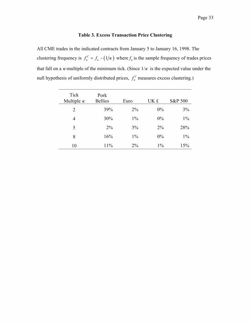
contracts. Clustering is most extreme (on κ = 2) in the pork belly contract. There is

modest clustering on κ= 5 for the S&P contract, while the currency prices are not

strikingly clustered.

Economic explanations for clustering vary. Harris (1994); Harris (1991) suggest

that negotiating parties may adopt a supra-minimum tick convention as a device for

reducing the number of rounds of bargaining. It is also suggested, however, that when

there are barriers to entry in the provision of liquidity services, clustering may serve as an

implicit collusive coordination mechanism (Kandel and Marx (1997) and Dutta and

Madhavan (1997)). This has been most strongly alleged for the Nasdaq dealer market

prior to the reforms in the mid 1990s.9

Hasbrouck (1999b) suggests that quote clustering be attributed to an implicit

effective tick. The effective tick, denoted Kt, is a natural multiple of the minimum tick

that arises as a trading convention or from individual preference. Clustering is imposed

on the (unobserved) bid and ask quotes by using generalized rounding functions:

[ ][ ]

Floor ,

Ceiling ,t t

t t

B M C K

A M C

= −

= +t

tK (11)

where Kt denotes the tick-multiple to which rounding will occur. In economic terms, Kt is

the implicit tick size. (For example, Kt = 2 implies rounding to even numbers.) While Kt

might be modeled in a very general fashion, the specifications estimated here will allow

for only two possible values: one (that is, the regular tick increment) and κ, a single

dominant multiple. As in Hasbrouck (1999b), it is convenient to assume an i.i.d.

Bernoulli distribution:

( )1, w. prob. 1

, w. prob. t

kK

kκ−

=

(12)

The Bernoulli probability parameter k may be interpreted as the clustering intensity. It is

distinct from the proportion of prices that occur on κ-tick multiples because some of

these occurrences would arise with simple (unclustered) rounding. The prior for k was

Beta(a, b) with , i.e., uniform between zero and one. 1/ 2a b= =

d. Summary

The full model consists of efficient price dynamics given in equation (8); the

implicit tick specification (12); the rounding transformation for the bid and ask quotes

9 The literature on clustering at Nasdaq is large. Key references include Christie, Harris, and Schultz (1994); Schwert (1997).

(11); and the transaction price realization (10). The observed data are the trade prices and

volumes { },tP volumet . The latent data are the efficient prices, trade direction indicators

and implicit tick sizes { }, ,t t tm q K . The model parameters are { }20, , , ,...,u JC kσ λ λ . The

clustering statistics reported above suggest taking κ= 2 for the pork belly contract

(“clustering on even prices”) and κ= 5 for the S&P contract. The currency contract prices

are not markedly clustered, but for the sake of estimating all specifications in parallel for

all contracts, I allow κ= 5.

From a structural economic perspective, the components of the model strongly

resemble other pre-existing empirical formulations of the sequential trade models. The

specification of the efficient price and related trade impacts (8) is similar to those used in

Glosten and Harris (1988), George, Kaul, and Nimalendran (1991); Hasbrouck (1991b),

Huang and Stoll (1994); Huang and Stoll (1997) and Madhavan, Richardson, and

Roomans (1997), among others. Except in the framework of Glosten and Harris,

however, the transaction price is a linear function of other structural variables. In the

present model, the mapping from efficient to transaction prices is mediated by the

nonlinear and stochastic rounding transformations that generate bids and asks.

5. Application to the futures data

The comprehensive model described in the last section was estimated for the four

representative contracts.

a. Parameter estimates.

reports parameter estimates. From an economic viewpoint, the most

interesting are those that asses trade impacts (the λs). For brevity, only the sums are

reported. The sums of λIntercept and λSlope are positive, with the exception of λSlope for the

UK £. The estimated trade effects may be characterized in two ways. First,

graphs the implied price impact functions. The vertical scale is approximately the

proportional price change in basis points associated with a purchase of a given number of

contracts. This is the cumulative impact (i.e., through lag 5), although the changes for all

contracts were substantially complete after the second period. For a trade of a given size,

Table 4

Figure 2

the price impact is relatively large for the pork belly contract, but low for the currency

and S&P contracts.

Secondly, recall that the efficient price dynamics are the given by the linear

specification in eq.(8). The coefficient of determination in this specification is a useful

summary measure of the relative importance of trades in explaining (efficient) price

volatility. This coefficient is denoted , by analogy with the usual regression R2.

The logic of the sequential trade models suggests this is a summary measure of

information asymmetry (Hasbrouck (1991b)). reports the estimates. They are

relatively high for the pork belly contract (61%), the Euro (53%), and the UK £ (67%),

but lower for the S&P (8%). To put this in context, a corresponding value for an NYSE

equity might be around 30-40% percent (Hasbrouck (1991b)).

2,m TradesR∆

Table 4

These interpretations are contingent on the assumption that the estimated trade

impacts are permanent. In this context, it must be admitted that the models are short-run

specifications. They may not detect reversals or reversions that occur over intervals

longer than the five lagged trades, as might be implied by inventory control. Reversions

would, of course, imply that the estimated permanent impacts are overstated.

Estimates of cost parameter C are dramatically lower than the corresponding

estimates for the basic Roll model (cf. Table 2). In fact, graphs of the C posteriors for the

present model (not shown) suggest that the bulk of the probability mass was quite near

zero. Alternative estimates (not shown) indicate that for the present model, when C is

constrained to zero, estimates of other parameters are little affected.

These findings admit a simple explanation. In the present model, bid and ask

quotes arise from rounding transformations applied to latent continuous variables

(including C). That the C posteriors are massed near zero suggests that the rounding

transformations suffice to account for the observed data. Alternatively, it appears that C

is so small relative to the tick size, that it cannot be well-characterized by the relatively

coarse price data.

The estimates of clustering intensity parameter k are generally consistent with the

relative clustering propensities described in Table 3: high for the pork belly and S&P

contracts; low for the currency contracts.

b. Discussion

The economic models of sequential trade identify permanent trade price impacts

with asymmetric information, private information that can be revealed in the price only

through trade. From this perspective, it is perhaps not surprising that a significant

proportion of volatility in the pork belly market originates from trades. There are, for this

contract, few alternative sources of price discovery.

In currency markets, however, the prevailing view ascribes a distinctly subsidiary

role for futures trading.10 Lyons (2001) comments, “In FX … the futures market is much

smaller than the spot market; it is unlikely that a significant share of price determination

occurs there.” The futures contract is often supposed to serve as a hedging and

speculation vehicle for participants too small to obtain easy access to the larger market.

One would therefore expect currency futures prices to follow passively the path

established in the interbank market. From this perspective, the high explanatory power of

trades is surprising.

The interbank market, however, is a low-transparency venue. The public record of

the interbank market is limited to indicative (nonfirm) bids and offers. Trades that occur

on the electronic book systems are visible only to other subscribers (essentially the large

intermarket banks themselves). Neither trades occurring directly between two participants

nor those mediated by brokers are publicly reported. The usefulness of the Reuters

indicative quotes as a timely, high-resolution signal for futures price discovery appears

doubtful. It seems reasonable to hypothesize that some trades in the futures market are

driven by information that may have originated in the interbank market (such as

knowledge of a recent interbank trade), and is “private” in the sense of not being widely

10 Recent microstructure studies of the latter include Lyons (1997); Lyons (1995); Goodhart, Ito, and Payne (1996) and Evans (2002).

reported. Although remaining (in a sense) a subsidiary player in this market, the futures

market may be serving as the primary forum of public price discovery.

For the S&P contract, the quantity-impact functions ( ) and the

values ( ) suggest a role for trades that is extremely, perhaps implausibly, low.

While the cash market exists as a meaningful alternative for price discovery, the stock

index futures market is customarily viewed as originating the primary signals of common

factor equity movements. Both the numerous studies documenting index price leadership

in the futures markets, and the studies that address regulatory concerns support this view.

2,m tradesR∆Figure 2

Table 4

In considering model adequacy for this contract, it is noteworthy that the index

futures market is substantially more active than the others. Section 2 noted an average

intertrade time of five seconds and raised the possibility of associated informational

delays. In principle, estimation is not affected by real-time frequency of trading.

However, high activity undoubtedly places stress on the reporting and data collection

systems. This increases the likelihood that the reported transactions are not correctly

sequenced. The noise introduced by sequencing errors might well attenuate the estimated

trade impacts.

Finally, trade price impact studies in equity markets generally find asymmetries

between purchases and sales with purchases having the larger impact (Holthausen,

Leftwich, and Mayers (1987); Holthausen, Leftwich, and Mayers (1990); Chan and

Lakonishok (1993); Chan and Lakonishok (1995)). This possibility suggests generalizing

eq. (8) to:

(13) 0 0

J J

t t j j t j t j j t j tj j

m q v q vλ λ+ + − −− − − −

= =

∆ = + +∑ ∑ u

)where and (0,t tq Max q+ = ( )0,tq Min q− = t are the positive and negative parts of qt. To

investigate this specification without incurring the complexity of a full Gibbs sampler, eq.

(13) was estimated using the qt generated in the estimation of the symmetric model. The

distributions of the buy and sell impact coefficients ( )and j jλ λ+ − were found to be very

similar.

6. Other extensions and modifications

The MCMC approach is sufficiently general to accommodate numerous useful

generalizations of the present models, including random costs of quote exposure,

stochastic volatility, and stochastic liquidity. Such extensions are facilitated by the

modularity of the MCMC framework. The basic building block is a draw (simulation)

from a “full conditional” density. In such a simulation, with the exception of the

particular variable being drawn, all other latent data and parameters, including those that

are stochastic in the full model specification, are provisionally taken as fixed.

A model may offer great economic appeal and even simplicity in its conditional

distributions, however, and still severely tax the ability of the data to meaningfully

identify the parameters. Estimates of costs and trade impacts in the present family of

models, for example, are sensitive to how discreteness and clustering are modeled.

As a further example, it is sensible to generalize the Roll model to allow

stochastic costs of quote exposure, i.e. to replace the time-invariant parameter c with a

stochastic process { }tc . It is certainly possible to reliably estimate such models when the

bid and ask quotes are observed, as in U.S. equities (Hasbrouck (1999a)) or foreign

exchange (Hasbrouck (1999b)).

Estimation is more difficult, however, when inference is attempted solely from

transaction prices. With the present data, for example, I attempted to estimate models

under the assumption that ( ) (. . .

2log ~ ,i i d

t cC N )cµ σ . The Gibbs samplers exhibited poor

mixing and convergence properties. This is perhaps not surprising. As in the basic Roll

model, the only nonzero second-order moments of price changes are the variance and

first-order autocovariance. These are obviously insufficient to identify the three

parameters { }2 2, ,c c uµ σ σ . In fact, identification requires fourth moments of price changes,

and, for determining distributional properties, eighth moments. Even when these

moments exist, sampling may be problematic.11

11 Alternatively, Ball and Chordia (2001) estimate a modification of a spread model suggested in Hasbrouck (1999a) that allows for autoregressive dependence in Ct. The

7. Conclusions

This paper proposes and implements powerful strategies to estimate empirical

microstructure models when the data consist of trade prices or alternatively, prices and

volumes. The specifications apply the signed return/signed order flow regressions

common in equity market studies to a setting in which there is no record of the quotes,

and therefore no straightforward way to sign trades as buyer- or seller-initiated. The

analysis is made possible by recent advances in Markov chain Monte Carlo estimation

(MCMC), which simplify inference in dynamic latent (unobserved) variable models. In

the present applications, the latent data are the trade signs. These are simulated,

conditional on the structure of the model and the observed data. The techniques are

Bayesian, but except in one respect (noted below) the priors used in the analyses are not

informative.

The paper presents an analysis of four representative futures contracts traded on

the Chicago Mercantile Exchange: pork bellies, the S&P Composite Index and two

currency contracts (the Euro and the UK £). The first application involves a variant of the

Roll (1984) model of transaction prices subject to bid-ask effects. For the data samples in

this paper, for comparison purposes, this model can also be estimated using the standard

moment-based approaches. For all contracts, both MCMC and moment approaches yield

similar estimates of the long-run volatility. The MCMC estimates of the effective

execution costs (the half-spread), however, are substantially smaller than the

corresponding moment estimates. This appears to reflect the fact that the moment

approach attributes all of the sample price-change autocovariance to the execution cost.

The MCMC approach does not force this attribution. As there are no direct observations

of the parameter, it is not possible to say for certain which estimate is closer to the truth.

It is worth noting, however, that if the model is correctly specified, the MCMC parameter

posteriors are exact small-sample distributions. The moment estimates in contrast are

valid only asymptotically, and may therefore be less robust in finite samples.

smoothing in this model appears to greatly enhance identification and performance of the Gibbs sampler.

The only respect in which the MCMC parameter priors are informative is that the

execution cost is constrained to be positive. This property is economically sensible.

Furthermore, the ability to estimate the Roll model subject to this requirement extends the

usefulness of this model to the many data samples in which moment estimates are

infeasible. In monthly samples of daily stock return data, for example, only about half the

samples yield feasible estimates. Thus, the MCMC approach shows promise in

establishing execution cost estimates in historical and international security datasets

which contain only transaction prices. Hasbrouck (2003) shows that Gibbs estimates of

execution cost based on daily CRSP data are highly correlated with estimates derived

from detailed trade and quote (NYSE TAQ) data from 1993 to 2001. Furthermore, the

Gibbs cost estimates constructed for the full daily CRSP sample (1962 onwards) are

positively related to excess returns.

The full specification estimated in this paper is a structural model of bid and ask

quotes and trades that incorporates discreteness, clustering and asymmetric information.

In application to the four contracts, several significant results emerge.

First, the estimates imply statistically and economically significant effects of

signed orders on prices for the pork belly, Euro and pound contracts. If these order

impacts are permanent, the estimates suggest that roughly half of the long-term price

volatility in these contracts is attributable to trades, and by implication, the private

information signals contained in these trades. The present specifications are short term,

however, covering only five lagged trades. They lack the power to detect reversions or

reversals in the price impacts extending over significantly longer intervals, as might be

implied by inventory effects. For the S&P contract, estimated order impacts are low, and

less than ten percent of the volatility can be attributed to trades.

This first result is broadly consistent with empirical analyses of equities (which

are based on richer data records). Taking the order impact coefficients as measures of

liquidity, the S&P contract is the most liquid. An order of roughly 50 contracts

(corresponding to roughly $16.5 Million in underlying value) moves the price by only

about one basis point. The pork belly contract is the least liquid: one contract (about

$23,000 in underlying value) moves the price by about ten basis points. The currency

contracts lie between these extremes.

Second, the non-informational costs of market making are substantially smaller

than the tick size (price increment). The relative coarseness of the price data precludes

precise estimation.

Third, the estimates imply price clustering (affinity for natural multiples of the

minimum tick) that is very strong for the pork belly contract, moderate for the S&P

contract and negligible for the currency contracts. It is not determined whether this

clustering arises from negotiation-cost minimization or market power of floor traders.

The relatively high liquidity found for the S&P contract is unsurprising. This

market is widely acknowledged to be extremely active. An index, furthermore, diversifies

the private information found in the individual components (Subrahmanyam (1991)). The

low estimated trade impacts found in the present analysis, however, might also result

from incorrect trade sequencing, due to a reporting system that is taxed by the rapid pace

of activity.

For the currency contracts, the strong contribution of trades to price volatility

suggests that that futures trading contributes significantly to the price discovery process.

This runs counter to the conventional wisdom that price determination in foreign

exchange occurs in the interbank spot/forward market. Transparency in the interbank

market, however, is low. Given that interbank trades are not reported, it is perhaps not

surprising that the publicly-reported (though smaller) futures trades play a substantial role

in price discovery.

Finally, the present models analyses by no means exploit the full potential of the

approach. The structure of a Gibbs sampler is essentially modular, and adding a new

feature often involves little more than adding a new step in each sweep. Extensions that

might be desirable in some applications would include stochastic volatility and multiple

securities. Furthermore, the present techniques are potentially applicable not only to

security markets, but also to markets for nonfinancial assets, products and services.

References

Ball, C.A., and T. Chordia. "True Spreads and Equilibrium Prices." Journal of Finance,

56 (2001), 1801-35.

Carlin, B. P., and T. A. Louis. Bayes and Empirical Bayes Methods for Data Analysis.

London: Chapman and Hall (1996).

Casella, G., and E.I. George. "Explaining the Gibbs Sampler." The American Statistician,

46 (1992), 167-90.

Chan, J., and J. Lakonishok. "Institutional Trades and Intraday Trade Price Behavior."

Journal of Financial Economics, 33 (1993), 173-99.

Chan, J., and J. Lakonishok. "The Behavior of Stock Prices Around Institutional Trades."

Journal of Finance, 50 (1995), 1147-74.

Chib, S., and E. Greenberg. "Markov Chain Monte Carlo Simulation Methods in

Econometrics." Econometric Theory, 12 (1996), 409-31.

Christie, W.G., J.H. Harris, and P.H. Schultz. "Why Did NASDAQ Market Makers Stop

Avoiding Odd-Eighth Quotes?" Journal of Finance, 49 (1994), 1841-60.

Dutta, P.K., and A.M. Madhavan. "Competition and Collusion in Dealer Markets."

Journal of Finance, 52 (1997), 245-76.

Easley, D., and M. O'Hara. "Price, Trade Size, and Information in Securities Markets."

Journal of Financial Economics , 19 (1987), 69-90.

Easley, D., and M. O'Hara. "Order Form and Information in Securities Markets." Journal

of Finance, 46 (1991), 905-27.

Easley, D., and M. O'Hara. "Adverse Selection and Large Trade Volume: The

Implications for Market Efficiency." Journal of Financial and Quantitative

Analysis, 27 (1992a), 185-208.

Easley, D., and M. O'Hara. "Time and the Process of Security Price Adjustment." Journal

of Finance, 47 (1992b), 576-605.

Engle, R.F. "Bayesian Analysis of Stochastic Volatility Models: Comment." Journal of

Business and Economic Statistics, 12 (1994), 395-96.

Evans, M.D.D. "FX Trading and Exchange Rate Dynamics." Journal of Finance, 57

(2002). 2405-2447.

Ferguson, M.F., S.C. Mann, and L.J. Schneck. "Concentrated Trading in the Foreign

Exchange Futures Markets: Discretionary Liquidity Trading or Market Closure."

Journal of Futures Markets, 18 (1998), 343-62.

Gamerman, D. Markov Chain Monte Carlo. New York: Chapman and Hall (1997).

George, T.J., G. Kaul, and M. Nimalendran. "Estimation of the Bid-Ask Spread and Its

Components: a New Approach." Review of Financial Studies, 4 (1991), 623-56.

Gilks, W. R., S. Richardson, and D. J. Spiegelhalter. "Introducing Markov Chain Monte

Carlo." in Markov Chain Monte Carlo in Practice, W. R. Gilks, S. Richardson,

and D.J. Spiegelhalter, eds. London: Chapman and Hall (1996).

Glosten, L.R., and L.E. Harris. "Estimating the Components of the Bid/Ask Spread."


Glosten, L.R., and P.R. Milgrom. "Bid, Ask, and Transaction Prices in a Specialist

Market With Heterogeneously Informed Traders." Journal of Financial

Economics, 14 (1985), 71-100.

Goodhart, C., T. Ito, and R. Payne. "One Day in June 1993: A Study of the Working of

the Reuters 2000-2 Electronic Foreign Exchange Trading System." in The

Microstructure of Foreign Exchange Markets, J. A. Frankel, G. Galli, and A.

Giovannini, eds. Chicago: University of Chicago Press (1996 ).

Hamilton, J.D., 1994. Time Series Analysis. (Princeton: Princeton University Press).

Harris, L.E. "Estimation of Stock Price Variances and Serial Covariances From Discrete

Observations." Journal of Financial and Quantitative Analysis, 25 (1990a), 291-

306.

Harris, L.E. "Statistical Properties of the Roll Serial Covariance Bid/Ask Spread

Estimator." Journal of Finance, 45 (1990b), 579-90.

Harris, L.E. "Stock Price Clustering and Discreteness." Review of Financial Studies, 4

(1991), 389-415.

Harris, L.E. "Minimum Price Variations, Discrete Bid-Ask Spreads, and Quotation

Sizes." Review of Financial Studies, 7 (1994), 149-78.

Harris, L. E. "Decimalization: A Review of the Arguments and Evidence." University of

Southern California (1997a).

Harris, L. E. "Does a Large Minimum Price Variation Encourage Order Exposure?"

School of Business Administration, University of Southern California (1997b).

Hasbrouck, J. "Trades, Quotes, Inventories, and Information." Journal of Financial

Economics, 22 (1988), 229-52.

Hasbrouck, J. "Measuring the Information Content of Stock Trades." Journal of Finance,

46 (1991a), 179-207.

Hasbrouck, J. "The Summary Informativeness of Stock Trades: An Econometric

Analysis." Review of Financial Studies, 4 (1991b), 571-95.

Hasbrouck, J. "Using the TORQ Database." New York Stock Exchange (1992).

Hasbrouck, J. "Modeling Microstructure Time Series." in Handbook of Statistics 14:

Statistical Methods in Finance, G. S. Maddala and C.R. Rao, eds. Amsterdam:

Elsevier North Holland (1996a).

Hasbrouck, J. "Order Characteristics and Stock Price Evolution: an Application to

Program Trading." Journal of Financial Economics, 41 (1996b), 129-49.

Hasbrouck, J. "The Dynamics of Discrete Bid and Ask Quotes." Journal of Finance, 54

(1999a), 2109-42.

Hasbrouck, J. "Security Bid/Ask Dynamics With Discreteness and Clustering: Simple

Strategies for Modeling and Estimation." Journal of Financial Markets, 2

(1999b), 1-28.

Hasbrouck, J. "Trading Costs and Returns for US Equities: the Evidence From Daily

Data." Stern School of Business New York University (2003).

Hasbrouck, J., and T.S.Y. Ho. "Order Arrival, Quote Behavior, and the Return-

Generating Process." Journal of Finance, 42 (1987), 1035-48.

Holthausen, R.W., R.W. Leftwich, and D. Mayers. "The Effect of Large Block

Transactions on Security Prices." Journal of Financial Economics, 19 (1987),

237-67.

Holthausen, R.W., R.W. Leftwich, and D. Mayers. "Large Block Transactions, the Speed

of Response, and Temporary and Permanent Stock Price Effects." Journal of

Financial Economics, 26 (1990), 71-95.

Huang, R., and H. Stoll. " The Components of the Bid-Ask Spread: a General Approach."

Review of Financial Studies, 10 (1997), 995-1034.

Huang, R.D., and H.R. Stoll. "Market Microstructure and Stock Return Predictions."


Jacquier, E., N.G. Polson, and P.E. Rossi. "Bayesian Analysis of Stochastic Volatility

Models." Journal of Business and Economic Statistics, 12 (1994), 371-89.

Jones, C. S. "The Dynamics of Stochastic Volatility: Evidence From Underlying and

Options Markets." Simon School of Business Rochester University (2002).

Kandel, E., and L.M. Marx. "NASDAQ Market Structure and Spread Patterns." Journal

of Financial Economics, 45 (1997), 61-89.

Kim, C.-J., and C. R. Nelson. State-space models with regime switching. Cambridge,

Massachusetts: MIT Press (2000).

Kim, S., N. Shephard, and S. Chib. "Stochastic Volatility: Likelihood Inference and

Comparison With ARCH Models." Review of Economic Studies, forthcoming

(1998).

Laux, P.A., and A.J.Jr. Senchack. "Bid-Ask Spreads in Financial Futures." Journal of

Futures Markets, 12 (1992), 621-34.

Lee, C.M.C., and M.J. Ready. "Inferring Trade Direction From Intraday Data." Journal

of Finance, 46 (1991), 733-46.

Locke, P.R., and P.C. Venkatesh. "Futures Market Transactions Costs." Journal of

Futures Markets, 17 (1997), 229-45.

Lyons, R.K. "Tests of Microstructural Hypotheses in the Foreign Exchange Market."


Lyons, R.K. "A Simultaneous Trade Model of the Foreign Exchange Hot Potato."

Journal of International Economics, 42 (1997), 275-98.

Lyons, R. K. The Microstructure Approach to Foreign Exchange Rates. Cambridge, MA:

MIT Press (2001).

Ma, C.K., R.L. Peterson, and R.S. Sears. "Trading Noise, Adverse Selection and Intraday

Bid-Ask Spreads in Futures Markets." Journal of Futures Markets, 12 (1992),

519-38.

Madhavan, A., M. Richardson, and M. Roomans. "Why Do Security Prices Change?"


Manaster, S., and S.C. Mann. "Life in the Pits: Competitive Market Making and

Inventory Control." Review of Financial Studies, 9 (1996), 953-75.

O'Hara, M. Market Microstructure Theory. Cambridge, MA: Blackwell Publishers

(1995).

Odders-White, E. R. "On the Occurrence and Consequences of Inaccurate Trade

Classification." University of Wisconsin (1997).

Roll, R. "A Simple Implicit Measure of the Effective Bid-Ask Spread in an Efficient

Market." Journal of Finance, 39 (1984), 1127-39.

Schwert, G.W. "Symposium on Market Microstructure: Focus on NASDAQ." Journal of

Financial Economics, 45 (1997), 1-8.

Shephard, N. "Fitting Nonlinear Time-Series Models With Applications to Stochastic

Variance Models." Journal of Applied Econometrics, 8 (1993), S135-S152.

Smith, T., and R.E. Whaley. "Estimating the Effective Bid/Ask Spread From Time and

Sales Data." Journal of Futures Markets, 14 (1994), 437-55.

Subrahmanyam, A. "A Theory of Trading in Stock Index Futures." Review of Financial

Studies, 4 (1991), 17-51.

U.S. Securities and Exchange Commission. 2001. Final rule: Disclosure of order routing

and execution practices.

Table 1. Contract Descriptions and Summary Sample Statistics

Contracts traded on the Chicago Mercantile Exchange for the indicated underlying and

maturity.

Contract

Pork Bellies Euro FX UK£ S&P 500

Expiration month Feb. 2000 Sep. 1999 Sep. 1999 Sep. 1999

Trading sample month Sep. 1999 Aug. 1999 Aug. 1999 Aug. 1999

Number of Trading Days 20 22 22 22

Total Number of Trades 3,882 9,869 9,414 106,402

Average Price 57.83 1.06 1.61 1,331.67

Price Units Cents/Lb US$/Euro US$/UK£ Index Pts

Tick 0.025 0.0001 0.0002 0.1

Average Tick/Price 0.043% 0.009% 0.012% 0.008%

Size of Contract 40,000 Lb 125,000 Eu 62,500 £ $250 x Index

Average Dollar Value ($1,000) 23.1 132.8 10.05 332.9

Std. Dev. of price change (log price × 10,000) 20.6 1.9 1.67 2.5

Std. Dev. of price change (ticks) 4.79 1.99 1.3 3.30

Average daily trades 194 449 428 4,836

Avg time between trade (sec.) 70.8 53.9 56.5 5.1

Distribution of trade sizes:

Min 1 1 1 1

25%’ile 1 2 1 2

Median 2 4 3 6

75%’ile 3 10 8 18

Max 140 420 374 713

Table 2. Estimates of the Roll Model.

Sample of CME contracts described in Table 1. σu is the standard deviation of the log

efficient price changes; c is the (log) half-spread; C is the half-spread in ticks. Estimates

labeled “Bayes, q simulated” are Gibbs sampler estimates in which the trade direction

indicators q are conditionally simulated. Results are based on 10,000 sweeps of the

sampler, with the first 2,000 discarded. Standard errors of the posterior means (SEM’s)

are corrected for autocorrelation in the draws (using spectral averages). The alternate

estimates labeled “Bayes, q fixed” are Gibbs sampler estimates in which the q are

assigned using a tick rule. Moment estimates are the conventional autocovariance-based

estimates of the model.

Primary Estimates Alternative Estimates

Bayes, q simulated

Moment Bayes,

q fixed

Contract Parameter Posterior

Mean SEM Posterior Std. Dev.

Point Estimate

Posterior Mean

Pork Belly

10,000uσ × 20.24 0.0118 0.312 19.41

20.58

10,000c× 2.52 0.0516 0.930 4.86 9.22

C (ticks) 0.58 0.0119 0.215 1.12 2.13

Euro 10,000uσ × 1.86 0.0005 0.016 1.79 1.87

10,000c× 0.17 0.0033 0.053 0.40 0.24

C (ticks) 0.18 0.0035 0.057 0.43 0.25

UK £ 10,000uσ × 1.60 0.0007 0.018 1.54 1.67

10,000c× 0.34 0.0017 0.036 0.47 0.24

C (ticks) 0.28 0.0014 0.029 0.37 0.19

S&P 10,000uσ × 2.47 0.0001 0.006 1.30 2.48

10,000c× 0.13 0.0005 0.013 1.49 3.46

C (ticks) 0.17 0.0006 0.017 1.99 4.61

Table 3. Excess Transaction Price Clustering

All CME trades in the indicated contracts from January 5 to January 16, 1998. The

clustering frequency is 1f fκ κ κ= − where fκ is the sample frequency of trades prices

that fall on a κ-multiple of the minimum tick. (Since 1/κ is the expected value under the

null hypothesis of uniformly distributed prices, Cfκ measures excess clustering.)

( )C

Tick Multiple κ

Pork Bellies Euro UK £ S&P 500

2 39% 2% 0% 3%

4 30% 1% 0% 1%

5 2% 3% 2% 28%

8 16% 1% 0% 1%

10 11% 2% 1% 15%

Table 4. Estimates of the Clustered Asymmetric Information Model

Sample of CME contracts described in Table 1. The log efficient price dynamics are

where 5

0t t i i t iim q vλ− −=

∆ = +∑ tu ( ), ,i i Intercept i Slopeλ λ λ= and ( )1t i tv volume−′= .

is the explained variance in this specification. C is the implicit quote exposure cost; k is the clustering intensity; κ is the clustering multiple. Estimates are based on 2,000 Gibbs sweeps with the first 400 discarded. Standard errors of the posterior means (SEM) are corrected for autocorrelation in the draws (using spectral averages).

2,m TradesR∆

Contract Parameter Post. Mean SEM Post. Std. Dev. Pork Belly 10,000uσ × 13.4926 0.0130 0.2096 (κ= 2) C (ticks) 0.3996 0.0200 0.1943 k 0.7839 0.0004 0.0101

, 10,000i Interceptλ ×∑ 6.3902 0.0909 1.4365

, 10,000i Slopeλ ×∑ 1.9517 0.0456 0.7812

2

,m TradesR∆ 0.6113 0.0007 0.0089 Euro 10,000uσ × 1.3115 0.0006 0.0119 (κ= 5) C (ticks) 0.0143 0.0012 0.0136 k 0.0258 0.0006 0.0061

, 10,000i Interceptλ ×∑ 2.4854 0.0088 0.1068

, 10,000i Slopeλ ×∑2

0.0110 0.0017 0.0237

,m TradesR∆ 0.5333 0.0003 0.0053 UK £ 10,000uσ × 1.0258 0.0006 0.0106 (κ= 5) C (ticks) 0.0077 0.0006 0.0076 k 0.0023 0.0001 0.0008

, 10,000i Interceptλ ×∑ 1.9128 0.0057 0.0775

, 10,000i Slopeλ ×∑2

-0.0197 0.0018 0.0242

,m TradesR∆ 0.6658 0.0003 0.0049 S & P 10,000uσ × 2.2703 0.0012 0.0126 (κ= 5) C (ticks) 0.0841 0.0201 0.1906 k 0.3179 0.0004 0.0042

, 10,000i Interceptλ ×∑ 0.4535 0.0132 0.1299

, 10,000i Slopeλ ×∑2

0.0767 0.0006 0.0098

,m TradesR∆ 0.0783 0.0028 0.0262

Figure 1. Posterior Distributions for the Basic Roll Model.

Sample of CME contracts described in Table 1. σu is the standard deviation of the log

efficient price changes; c is the (log) half-spread; C is the half-spread in ticks. Histograms

are based on 10,000 sweeps of the Gibbs sampler, with the first 2,000 discarded.

18 20 22 0 5 0 1 2

1.6 1.8 2 0 0.2 0.4 0 0.2 0.4

1.5 1.6 1.7 0 0.5 0 0.2 0.4

2.45 2.5σu×10,000

0 0.1 0.2c×10,000

0 0.2 0.4C (ticks)

Pork Bellies

Euro

UK

S&P 500

Figure 2. Implied Trade Price Impacts

Cumulative impact of a buy order on the log efficient price as a function of order size.

Estimates based on clustered asymmetric information model with trade impact terms

(through lag five). Dashed line indicates approximate tick size.

0 5 100

2

4

6

8

10

12Pork Bellies

Buy Size (Contracts)

Cum

Impa

ct (B

asis

Poi

nts)

0 20 40 600

0.5

1

1.5

2

2.5Euro

Buy Size (Contracts)C

um Im

pact

(Bas

is P

oint

s)

0 20 40 600

0.5

1

1.5

UK


Cum

Impa

ct (B

asis

Poi

nts)

0 50 1000

0.2

0.4

0.6

0.8

1

1.2S&P


Cum

Impa

ct (B

asis

Poi

nts)

Liquidity in the U - New York Universitypeople.stern.nyu.edu/jhasbrou/Research/Working Papers...Page...

Documents

Transcript of Liquidity in the U - New York Universitypeople.stern.nyu.edu/jhasbrou/Research/Working Papers...Page...