Liquidity and resolution of uncertainty in the European ...

Liquidity and resolution of uncertainty in the European

carbon futures market

Iordanis Angelos Kalaitzoglou, Boulis Maher Ibrahim

To cite this version:

Iordanis Angelos Kalaitzoglou, Boulis Maher Ibrahim. Liquidity and resolution of uncertaintyin the European carbon futures market. International Review of Financial Analysis, Elsevier,2015, 37, pp.89-102. <10.1016/j.irfa.2014.11.006>. <hal-01107956>

HAL Id: hal-01107956

https://hal.archives-ouvertes.fr/hal-01107956

Submitted on 9 Feb 2015

HAL is a multi-disciplinary open accessarchive for the deposit and dissemination of sci-entific research documents, whether they are pub-lished or not. The documents may come fromteaching and research institutions in France orabroad, or from public or private research centers.

L’archive ouverte pluridisciplinaire HAL, estdestinee au depot et a la diffusion de documentsscientifiques de niveau recherche, publies ou non,emanant des etablissements d’enseignement et derecherche francais ou etrangers, des laboratoirespublics ou prives.

https://hal.archives-ouvertes.fr

https://hal.archives-ouvertes.fr/hal-01107956

Liquidity and Resolution of Uncertainty in the European Carbon

Futures Market

Iordanis Angelos Kalaitzoglou

Audencia School of Management, Pres LUNAM, CFRM, Nantes 44312, France

e-mail: [email protected]

Boulis Maher Ibrahim

Accounting, Economics and Finance, Heriot-Watt University, Edinburgh EH14 4AS, UK

e-mail: [email protected], Tel: 00 44 (131) 451 3560

Abstract

We investigate whether liquidity introduces or helps resolve uncertainty in Phase

I and the first year of Phase II of the European Carbon futures market. We propose

a distinction between ‘absolute’ or overall liquidity and that which is ‘relative’ to

a benchmark. For this purpose, we suggest volume–weighted duration as a natural

measure of trading intensity as a proxy for liquidity, and we model it as a rescaled

temporal point process. The new model is called Autoregressive Conditional

Weighted Duration (ACWD) and is shown to outperform its discrete modelling

counterparts. Liquidity is found to play a dual role, with higher relative liquidity

introducing uncertainty and higher absolute liquidity accelerating uncertainty

resolution, thus, enhancing market efficiency.

JEL Classifications: C41, C46, G14, Q40

Keywords: Intraday Liquidity, Marked Duration, Temporal Marked Point Process, Carbon

Market

mailto:[email protected]

1

1. Introduction

This paper investigates whether liquidity introduces or facilitates the resolution of uncertainty.

If liquidity is linked to, or convey, information (Easley and O’Hara, 1992) some uninformed

traders who observe variations in liquidity might believe that there is price unresolved

information. Accordingly, some relative levels or variations of liquidity might induce

uncertainty (price volatility). Upon greater ambiguity aversion the magnitude of the resulting

volatility shock(s) would be expected to be greater. If liquidity exhibits such conditionality,

then higher liquidity episodes relative to ‘norm’ or benchmark levels (e.g., annual, daily, or

hourly averages, or levels dictated by uninformed investors) may induce uncertainty, while

high general norm or benchmark levels may help resolve uncertainty by accelerating

uncertainty resolution time. In this paper we recognise this likely dual role of liquidity, and use

it to motivate an explicit distinction between ‘absolute’ and ‘relative’ liquidity, which may

facilitate the determination of uncertainty. We model liquidity conditionality (parametrically)

and use the trades of higher relative liquidity identified by this modelling to test (non–

parametrically) whether this conditionality affects volatility.

From a microstructure point of view the market is seen as a price discovery and a liquidity

provision mechanism (O’Hara, 2011), where information (Bagehot, 1971; Kyle, 1985; Glosten

and Milgrom, 1985) and liquidity (Tinic 1972; Tinic and West, 1972; Benston and Hagerman,

1974) are the drivers of intraday price formation. Focusing on liquidity, relevant literature

recognises a transitory effect on price formation due to ‘inventory holding’ (Garman 1976;

Amihud and Mendelson, 1980; Stoll, 1978; Ho and Stoll, 1981, 1983). Without disregarding

this conventional role of liquidity, seen as a matching mechanism that results in transaction

costs and is positively related to asset prices, O’Hara (2003) identifies a more complex role

related to the risk of holding an asset. Specifically, systematic fluctuations in liquidity might

be related to the presence of price unresolved information (Easley and O’Hara, 1992). This

indicates that liquidity, as a non–price measure, conveys price related information

(Kalaitzoglou and Ibrahim, 2013b) and might thus affect perceptions of risk and risk premia.

If this risk is not fully diversifiable across assets, liquidity leakage (O’Hara, 2003) might

increase ambiguity–induced (Easley and O’Hara, 2010) volatility.

The question that naturally arises is how sophisticated the trading patterns of various market

participants are, and how they interact with each other. O’Hara (2003) argues that informed

traders continuously move a partially revealing price equilibrium according to new

information. Private or imperfect public information is continuously and partially revealed

through trades. Further, public information, when not perfect, increases ambiguity and is not

2

immediately incorporated into prices. Due to ambiguity, therefore, not everybody perceives the

same signal in the same way and, thus, prices need a period of time to adjust. During this

uncertainty resolution period, some uninformed traders observe and ‘learn’ from trading

history and act upon sufficiently strong accumulated information, according to their portfolio

needs, given that there is enough time till the information gets price resolved. They become

more informed to the remaining uninformed and can exploit the newly extracted information

but only within a limited time window till their advantage becomes obsolete. Their actions

temporarily increase liquidity, which might accelerate price resolution or increase uncertainty

and hence volatility. Consequently, this uncertainty resolution period can be thought of as a

‘time game’ among uninformed traders. Liquidity, therefore, cannot be considered

independently from price discovery since they interact affecting price formation. The price

discovery mechanism of the market can, thus, be seen as a continuously revealing price

equilibrium, where information dissemination is not an instantaneous event but interacts with

liquidity. Under this perspective, liquidity should exhibit some sort of conditionality.

Furthermore, organised markets are seen as a diverse information aggregation mechanism

(Kyle and Viswanathan, 2008), where liquidity might increase market efficiency (Hayek, 1945)

without necessarily increasing ‘price accuracy’ too.1 According to O’Hara (2003), they also

seem to implicitly recognise multiple roles for liquidity. Overall liquidity is understood to

improve market efficiency, since it enables the easier incorporation of price related signals into

prices. This implicitly assumes that information held by better informed agents is revealed

through trading signals and thus, conditionality in liquidity might induce uncertainty. In this

paper we explicitly distinguish between ‘absolute’ liquidity, defined as the overall volume of

trading, from ‘relative' liquidity, defined as different liquidity levels relative to a liquidity

benchmark. We investigate liquidity patterns, where relative liquidity might induce

uncertainty, the resolution time of which depends on absolute liquidity.

The first contribution of this paper is the explicit modelling of trading intensity (proxy for

liquidity) as a rescaled temporal point process. Engle and Russell (1998) describe the dynamics

of inter–arrival time of events as a dependent point process, and model it with the

Autoregressive Conditional Duration (ACD) model. However, duration alone is not always

sufficient in describing the intensity of trading, and event time needs to be modelled along with

other variables of interest called marks (e.g., trade price or trade volume/size). Following the

1 A less regulated, highly manipulated market might be more liquid and thus, more efficient, in terms of

incorporating manipulation into prices, yet assets are not necessarily priced according to fundamentals.

3

Autoregressive Conditional Intensity (ACI) framework of Russell (1999), Tay et al. (2004)

propose the Autoregressive Conditional Multinomial Duration (ACMD) model, which

describes durations and associated marks as a temporal marked point process with discrete

marks. Each state of a mark is thought of as a parallel point process, the realisation of which

depends on past information. In parallel, Russell and Engle (2005) develop the Autoregressive

Conditional Multinomial (ACM) framework, which jointly models arrival times and transition

probabilities among the different stages of an associated discrete mark. The major limitation of

these approaches is that marks with continuous distributions would require an infinite number

of states.

This paper, instead, shifts the focus from event (transaction) time to events defined by a unit

change in an associated mark. We use a kernel transformation of the mark to weigh or rescale

durations. This produces a new measure of the waiting time for the arrival of a unit quantity of

the mark. The new framework is called Autoregressive Conditional Weighted Duration

(ACWD), and is used to model volume weighted duration as a better measure of trading

intensity than duration alone. The conditional intensity (hazard function) of this natural

measure of trading intensity depends upon past transformed durations and measures the

instantaneous rate of the arrival time of a single unit of the mark. This extends the ACD

framework of Engle and Russell (1998) in the sense that it enables the modelling of a marked

point process as a univariate temporal point process.

The second contribution of this paper refers to the explicit distinction between ‘absolute’

and ‘relative’ liquidity and their differential impact on volatility and uncertainty resolution. We

investigate the intraday volatility impact of high trading intensity episodes in Phase I (2005-

2007) and the first year of Phase II (2008-2012) of the European Carbon market, identified in

Kalaitzoglou and Ibrahim (2013a). This market consists of distinct organised exchanges and

trading phases with notably different, but increasing, levels of overall liquidity for the same

commonly traded contracts. The total supply of traded emission allowances and credits is

regulated (capped) and, even though allowances could not be carried forward from Phase I to

Phase II (‘banking restriction’), there has been an over allocation of allowances since market

inception, affecting prices and liquidity.2 This provides an ideal setting for investigating

potentially different effects of the two types of liquidity defined above. In more detail, the new

model allows for a deeper insight on the creation, magnitude and length of these episodes,

2 See, for example, Alberola et al. (2008), Mansanet–Bataller and Pardo (2008) and Kalaitzoglou and Ibrahim

(2013a).

4

because it focuses on a richer measure of trading activity as a proxy for liquidity. An increase

(decrease) in volatility levels following a high trading intensity trade would indicate the

introduction (resolution) of price relevant information, and this would capture the volatility

impact of high relative liquidity. We further investigate the intraday resolution time of the

volatility impact of high trading intensity trades. A shorter (longer) resolution period, when

overall liquidity is higher, would indicate that higher absolute liquidity leads to increased

(decreased) market efficiency, in the sense of faster information dissemination and uncertainty

resolution.

To the extent that volume and duration convey information and liquidity, and inform

subsequent bid and ask price quote setting, the new measure of volume–weighted duration

relates directly to four of the five overlapping dimensions of liquidity: immediacy (speed of

order execution, clearing and settlement), resiliency (the speed with which prices recover from

a random uninformative shock), tightness (the cost of turning around a position within a short

period of time) and depth (the size of an innovation in aggregate quantity traded). It may relate

indirectly to breadth (numerous large orders) which could translate, at least partially, to faster

large or block trade execution.3 As higher ‘general’ trading activity is usually associated with

greater depth and lower trading costs (O’Hara, 2011; and Kalaitzoglou and Ibrahim, 2013b),

tightness and depth would be partially accounted for by a trading intensity measure, even

though the direction of causality (from spreads or depth to trading intensity, or vice versa) may

not be clear in a duration model without an explicit price dimension, such as the one suggested

here, although it could be extended to include this dimension.4

The results indicate that there exist strong liquidity momentums, which drive intraday

trading activity and price change volatility. Relatively higher trading intensity seems to be

followed by increased volatility, which needs at least 7 minutes to be price resolved. These

uncertainty shocks seem to be smaller in magnitude and to be absorbed relatively faster in more

liquid environments. This highlights a major difference between absolute and relative liquidity.

3 Hence we include block trades in our data sample. For definitions of the rather ‘slippery’ concept of liquidity

see, e.g., Kyle (1985), Grossman and Miller (1988) and Ranaldo (2001).

4 Asymmetric information microstructure models attribute trading costs, including the bid–ask spread, to

interacting information (‘permanent’) and liquidity (‘temporary’) related components that are further dissected

into order processing, asymmetric information, inventory–carrying (immediacy), and oligopolistic market

structure costs (Sarr and Lybek, 2002). Obviously, if price quote setting follows a ‘learning’ process from the

recent evolution of order flow then the speed and size of trades would inform subsequent (variable) trade cost

setting, and hence prices.

5

Higher relative liquidity is linked to higher presence of information and introduces uncertainty,

while higher absolute liquidity contributes to market efficiency, in the sense of lower in

magnitude, faster absorbed shocks.

The remainder of the paper is organised as follows; Section 2 presents the methodology,

Section 3 describes the data collection and manipulation, Section 4 discusses the empirical

findings, and Section 5 concludes.

2. Methodology

2.1 Time Rescaling

Let {𝑡0, 𝑡1, … , 𝑡𝑛, … } with 𝑡0 < 𝑡1 < ⋯ < 𝑡𝑛 < ⋯ , 𝑡 ∈ 𝑇, be the sequence of arrival times

of a type of event, such as transactions, of an asset A. N(t) is the counting function, counting

the number of events occurred by time t and 𝑚𝑖~(��, 𝜎𝑚2 ), 𝑚 ∈ 𝑀 denotes an associated mark.

Assuming that both the realisation time and the mark 𝑚 are conditional on past history 𝐹𝑖 ≔

(��𝑖, ��𝑖), i.e., a σ-algebra on 𝛺 = {𝑇𝑥𝑀}, where ��𝑖, ��𝑖 is the history of 𝑡 and 𝑚 up to event 𝑖,

and they formulate a temporal mark point process (henceforth t.m.p.p.) {(𝑡𝑖, 𝑚𝑖)} on {𝛺, 𝐹𝑖 , 𝑃},

where 𝑃: 𝐹 → [0,1] is a mapping of 𝐹 on [0,1]. The conditional joint density function of

{(𝑡𝑖, 𝑚𝑖)} is (𝑡𝑖, 𝑚𝑖)|𝐹𝑖−1~𝑓(𝑡𝑖, 𝑚𝑖|��𝑖−1, ��𝑖−1; 𝑐), where c is a vector of parameters. The

conditional expectations of arrival time and the associated mark can be derived from the

marginal density functions; 𝐸[𝑡𝑖|𝐹𝑖] = ∫ 𝑡

𝑇 𝑓(𝑡𝑖|𝐹𝑖−1)𝑑𝑡 and 𝐸[𝑚𝑖|𝐹𝑖] =

∫ 𝑚

𝑀 𝑓(𝑚𝑖|𝐹𝑖−1)𝑑𝑚.

In this paper, we shift focus from transactions to a unit quantity of associated marks. In the

majority of the market microstructure literature, the arrival time of events focuses on the arrival

of transactions or the submissions of orders. However, in some cases, such as inventory

position adjustment (e.g., Amihud and Mendelson, 1980), execution risk (e.g., Cohen et al.,

1980, 1981), or regret free price quotation (e.g., Madhavan et al., 1997), the waiting time up to

a certain event, other than the transaction itself, might be of greater importance. A convenient

measure could be the accumulated magnitude of mark, 𝑚, i.e., 𝜉(𝑡) = ∑ 𝑚𝑖𝑖,0<𝑡𝑖<𝑡 , over (0, 𝑡).5

Relevant literature (e.g., Tay et al., 2004) suggests the modelling of the conditional intensity

function of the t.m.p.p. as the collection of discrete temporal point processes (henceforth t.p.p.).

Despite allowing for the derivation of the marginal density functions, this approach is restricted

5 For example, a trader who submits a large order is exposed to execution risk due to insufficient liquidity or

market depth. In this case, she should be more interested in how long it is expected to take for a certain quantity

of the underlying asset to be traded, rather than what is the expected waiting time till the next transaction.

6

to a finite number of states of the associated mark, with the transition probabilities assumed to

follow a Markov chain. However, when the aggregated magnitude of a continuous mark is of

interest, the modelling of 𝐸[𝜉(𝑡)] would be more convenient. Depending on the independence

assumptions among the marks and the arrival times, 𝐸[𝜉(𝑡)] could be described by various

specifications (Daley and Vere-Jones, 2003). The expected aggregated magnitude of the

associated mark over a period of time could be defined as the expected number of events times

the expected value of the mark. Consequently, 𝐸[𝜉(𝑡𝑖)|𝐹𝑖−1] could be defined as

𝐸[𝑁(𝑡𝑖)|𝐹𝑖−1]𝐸[𝑚𝑖|𝐹𝑖−1] = ∫ 𝜆(𝑡𝑖|𝐹𝑖−1)𝑡+𝛥𝑡

𝑡𝑑𝑡 ∫ 𝑚

𝑀 𝑓(𝑚𝑖|𝐹𝑖−1)𝑑𝑚, where λ(·) is the

conditional intensity of arrival time.

In this paper we suggest an alternative formulation of 𝐸[𝜉(𝑡𝑖)|𝐹𝑖−1], by rescaling the arrival

time, t, of a certain event (e.g., transaction) with associated marks, to the arrival time, t*, of a

unit quantity of the associated mark. Assuming that the magnitude of the mark of the last event

(e.g., transaction) can be spread out in the time between two subsequent events, this is the

mapping 𝑡∗: 𝑇 ⨯ 𝑀 → 𝑇, where ( 𝑡𝑖, 𝑚𝑖) → 𝑡𝑖∗ ≔ 𝑡𝑖𝑔(𝑚𝑖) and 𝑔(𝑚𝑖) is a function of the

associated mark. The sequence {𝑡0∗, 𝑡1

∗, … , 𝑡𝑛∗ , … } with 𝑡0

∗ < 𝑡1∗ < ⋯ < 𝑡𝑛

∗ < ⋯ , 𝑡∗ ∈ 𝑇 is a t.p.p

and refers to the arrival time of a unit quantity of the associated mark (e.g., how long it takes

for price to change one tick, or for one unit of volume to be traded, …, etc.). Consequently, the

expected accumulated quantity of the mark over (0, 𝑡) would simply be the expected value of

the counting process 𝑁(𝑡∗), thus 𝐸[𝜉(𝑡𝑖)|𝐹𝑖−1] = 𝐸[𝑁(𝑡𝑖∗)|𝐹𝑖−1]. The rescaled process could

be fully described by its conditional intensity measure, which, assuming a function Y, is given

by (𝑌(𝑡𝑖)|𝐹𝑖−1) = 𝜆(𝑡𝑖𝑔(𝑚𝑖)|𝐹𝑖−1) = 𝜆(𝑡𝑖∗|𝐹𝑖−1) = 𝜆(𝑡𝑖

∗|𝑡0∗, 𝑡1

∗, … , 𝑡𝑖−1∗ ) =

lim𝛥𝑡→0

𝑃(𝑁(𝑡∗+𝛥𝑡)>𝑁(𝑡∗)|𝑡0∗ ,𝑡1

∗ ,…,𝑡𝑖−1∗ )

𝛥𝑡. This describes the probability of a unit mark (e.g., one contract

or one tick price change) to occur, given that it has not so far.

2.2 Autoregressive Conditional Weighted Duration (ACWD)

The new formulation proposed follows the ACD model of Engle and Russell (1998). First,

let 𝑑𝑖 = 𝑡𝑖 − 𝑡𝑖−1 denote the (raw) duration of event i, measured by the time (t) elapsed since

the preceding event at i-1, while 𝑥𝑖 denotes the diurnally adjusted duration. We suggest using

the normalised mark 𝑔(𝑚𝑖) = 𝐾(𝑢𝑖), as a scaling factor for the duration realisation process, to

formulate a new weighted duration variable 𝑧𝑖, with 𝜃𝑖 = 𝐸(𝑧𝑖|𝐹𝑖−1).

Consequently, the temporal marked point process (𝑥𝑖, 𝑚𝑖) is transformed into a temporal

point process (𝑌{𝑥𝑖, 𝑚𝑖}), with density function (𝑌{𝑥𝑖, 𝑚𝑖}|𝐹𝑖−1) = (𝑧𝑖|𝐹𝑖−1)~𝑓(𝑧𝑖|��𝑖−1; 𝜑),

where ��𝑖−1 is the history of z up to time i-1 and φ is a vector of parameters. In more detail,

using the following density kernel, 𝑧𝑖 could be defined as:

7

𝑧𝑖 = 𝑥𝑖 ∗ 𝐾(𝑢𝑖) (1)

𝐾(𝑢𝑖) = 𝑒𝑥𝑝 (−𝑢𝑖

2) (2)

𝑢𝑖 = (𝑚𝑖 − ��)/𝜎𝑚. (3)

The choice here of kernel, 𝐾(𝑢𝑖), is motivated by three advantages. First, the exponential

functional form accelerates (decelerates) time of transactions with a mark above (below) the

mean mark (��). Thus, it ‘discounts’ or ‘compounds’ duration by the distributional position of

the mark relative to the mean. Second, 𝑢𝑖 is a normalisation (z-score) of the mark and this

preserves the shape of the mark distribution (i.e., skeweness and kurtosis would still be present

if the mark’s distribution is skewed with fat tails). Finally, this normalisation smoothes or

reduces mark intra-day seasonality.6 The new variable (i.e., weighted duration, 𝑧𝑖) measures

the waiting time for the realisation of a unit mark. We model 𝑧𝑖 as:

𝑧𝑖 = 𝜃𝑖𝜀𝑖 (4)

𝜃𝑖 = 𝜃(𝑧𝑖−1, … , 𝑧1; 𝜑1) (5)

𝜀𝑖|𝐽𝑖~ 𝑖. 𝑖. 𝑑., 𝑤𝑖𝑡ℎ 𝑑𝑒𝑛𝑠𝑖𝑡𝑦 𝑓(𝜀𝑖|𝐽𝑖; 𝜑2) and 𝐸(𝜀𝑖|𝐽𝑖; 𝜑2) = 𝐸(𝜀𝑖) = 1 (6)

where 𝑧𝑡 is the weighted duration, calculated as in Eq. (1), 𝜃𝑖 is the expected value of 𝑧𝑖, 𝜀𝑖

is the error term, 𝐽𝑖 is an economically relevant threshold variable and φ’s are sets of

parameters. This model allows for various empirical specifications for the conditional mean

and the distribution to better fit the stylised facts of the market under investigation.

2.3 Instantaneous Liquidity

Although various marks can be used, we focus on non–price trading information and the

associated mark of interest is trade volume or size (i.e., number of contracts), 𝑣𝑖. Consequently,

the transformed variable is 𝑆𝑖 = 𝑥𝑖 ∗ 𝐾(𝑢𝑖), where 𝐾(𝑢) = 𝑒𝑥𝑝 (−𝑢𝑖

2) and 𝑢𝑖 = (𝑣𝑖 − ��)/𝜎𝑣.

This variable is an explicit measure of trading intensity as a proxy for liquidity, and measures

the waiting time for a single contract to be traded. The ACW for 𝑆𝑖 can be formulated as 𝑆𝑖 =

6 A graph showing the reduction in seasonality is available from the authors. Many alternative kernels are also

possible. The Gaussian, for example, is most commonly used for its desirable statistical properties (it has a

bandwidth equal to the standard deviation), although the Epanechnikov kernel may have optimal convergence

(most efficient) properties (see, e.g., Epanechnikov, 1969).

8

𝛩𝑖𝜀𝑖, where 𝛩𝑖 = 𝐸(𝑆𝑖|𝐹𝑖−1; 𝜑) = 𝛩(𝑆𝑖−1, … , 𝑆1; 𝜑1). Following Kalaitzoglou and Ibrahim

(2013b), the conditional mean is specified as

𝛩𝑖 = 𝜔 + ∑ 𝑎𝑗𝑆𝑖−𝑗𝑚𝑗=1 + ∑ 𝛽𝑗𝛩𝑖−𝑗

𝑞𝑗=1 , (7)

where 𝛩𝑖 is the conditional expected trading intensity, and 𝜀𝑖 is the so called standardised

trading intensity, given by the ratio 𝑆𝑖/𝛩𝑖. The conditional density function is a smooth

transition mixture of Weibull:

𝑓(𝜀𝑖|𝐽𝑖; 𝝉) =

(ℎ(𝐽𝑖: 𝝉) 𝑆𝑖⁄ )[𝑆𝑖𝛤(1 + 1 ℎ(𝐽𝑖: 𝝉)⁄ ) 𝛩𝑖⁄ ]ℎ(𝐽𝑖:𝝉)exp (−[𝑆𝑖𝛤(1 + 1 ℎ(𝐽𝑖: 𝝉)⁄ ) 𝛩𝑖⁄ ]ℎ(𝐽𝑖:𝝉)), (8)

where,

ℎ(𝐽𝑖: 𝝉) = 𝛾1 + (𝛾2 − 𝛾1) ∗ 𝐺1(𝐽𝑖: 𝑔1, 𝑗1) + (𝛾3 − 𝛾2) ∗ 𝐺2(𝐽𝑖: 𝑔2, 𝑗2), (9)

𝐺𝑘(𝑆𝑖: 𝑔𝑘, 𝑗𝑘) = (1 + 𝑒𝑥𝑝{−𝑔𝑘 ∗ (𝐽𝑖 − 𝑗𝑘)})−1. (10)

The shape parameter, ℎ(𝐽𝑖: 𝝉), of the mixture of Weibull distribution is a function, h, of the

threshold variable, Ji, which we represent by the first lag of S, and a vector of parameter

coefficients τ = (γ1 γ2 γ3 g1 g2 j1 j2), where, γ1, γ2, and γ3 are the shape parameters of the

Weibull distributions in three regimes of low, medium and high trade intensity determined by

the two threshold values j1 and j2 of the threshold variable Ji, and gk (k=1,2) is the smoothness

parameter between regimes. For every observation the overall shape parameter of the

distribution ℎ(𝐽𝑖 = 𝑆𝑖−1: 𝝉) is the weighted average of the shape parameters in the three

regimes, γ1, γ2, and γ3.7 The weights are determined by two smooth transition functions, G1 and

G2. Consequently, the conditional intensity (hazard function) of weighted durations, i.e. the

probability of a single contract to be traded given that it has not so far, is revised after every

transaction, providing a measure of instantaneous liquidity.

This modelling provides richer specifications for the conditional intensity over discrete

mark models, such as the ACMD of Tay et al. (2004) and the ACM–ACD of Russell and Engle

(2005). In Tay et al. (2004) only marks with discrete distributions are employed and the

associated durations are treated as parallel, independent point processes. The ACWD model

relaxes the independence assumption, by allowing a simultaneous modelling of both

7 The values that the shape parameters take on have direct implications on the arrival rate of unit marks (single

contracts). If γi = 1, the associated distribution is Exponential and the hazard function is approximately flat. This

indicates a rate of arrival of a single contract that does not change over time. If γi < 1, the Weibull distribution

and the associated hazard function have a monotonically decreasing slope. This indicates increased probability

of a single contract to be traded closer to the realization of the last event. Finally, if γi > 1, the Weibull distribution

is bell–shaped and the hazard function has an upward slope. This indicates that the probability of a single contract

arrival increases over time. The rates are only revised after the next transaction is observed.

9

continuous time and continuous marks. The latter is also a marginal improvement over ACM,

which only allows discrete marks to be considered.8

Estimation is conducted by maximising the log–likelihood employing the Broyden,

Fletcher, Goldfarb and Shanno (BFGS) algorithm with numerical derivatives and

heteroskedasticity robust errors. The model is compared to two parsimonious specifications of

the ACM–ACD and ACMD models. All models are fitted using the Box–Jenkins methodology

and relative performance is further tested through in– and out–of–sample forecast accuracy, as

additional ‘goodness of fit’ tests. (See the technical appendix for competing models,

forecasting setup and performance comparison measures.)

3. Data

3.1 The European Carbon Market9

Liquidity and its volatility impact are of particular importance in young and relatively

illiquid markets, such as the European Union Emissions Trading System (EU ETS). This

market exhibits some features that distinguish it from other markets. It employs a ‘cap and

trade’ system, where overall supply is politically regulated. This aims at a gradual increase in

prices, which should function as an incentive for reducing overall emissions. It is a relatively

new market that has gradually gained liquidity, with growing numbers of participants and

overall trading volume.10 Therefore, absolute liquidity is expected to contribute to higher

market efficiency. In contrast, market participants can trade the same standardised futures

contracts (European Union Allowance–EUA–futures) in overlapping trading mechanisms.

This market structure allows for liquidity and information exchange across trading venues.

Phase I Trading pattern variations might temporarily affect price formation due to liquidity

inflow, or permanently move prices as a result of pertinent information becoming available.

8 There is a trade-off between the two approaches. The modelling of marked durations using only discrete states

allows for the specification of the marginal distributions of both the duration and the states. In contrast, the ACWD

models marked durations as a single variable. The joint distribution is the distribution of a single variable, and the

conditional intensity (hazard function) depends on its past. The marginal distributions of duration and the mark

are indistinguishable, but this allows for the modelling of marks with continuous distributions in a convenient

way.

9 See the European Commission Climate Action website <http://ec.europa.eu/clima/policies/ets/index_en.htm>,

Convery and Redmond (2007) and Benz and Hengelbrock (2008) for further coverage on this market.

10 See, e.g., the growth in trading volume, the utility sector, and aviation inclusion (from January 2012) in reports

of organisations such as the World Bank (Cappor and Ambrosi, 2006; accessible at

<https://wbcarbonfinance.org/docs/>), and Mansanet–Bataller and Pardo (2008).

http://ec.europa.eu/clima/policies/ets/index_en.htm

https://wbcarbonfinance.org/docs/

10

Consequently, fluctuations in relative liquidity might have an opposing effect to absolute

liquidity by inducing noise and/or price relevant information.11 An explicit modelling of trading

activity should contribute to identifying potentially different price impact of absolute and

relative liquidity.

Although early literature evidently ignores the intraday trading activity dynamics, recent

studies highlight its contribution to price discovery and market maturity. Mizrach and Otsubo

(2014), for example, report that increasing liquidity in EU ETS is associated with increasing

price impact. Ibikunle et al. (2011) contend that this is not necessarily generated by increased

volume, but more likely by higher trading frequency. Bredin et al. (2014) confirm the price

impact of duration, but report a negative contemporaneous correlation between volume and

volatility. They conclude that liquidity effects dominate informed trading price impact.

Kalaitzoglou and Ibrahim (2013a) further investigate this issue and provide empirical evidence

that high trading intensity shocks induce increased trading activity episodes, mainly due to

increased volume. Independently of their link to contemporaneous volatility, high trading

intensity trades seem to induce higher volatility. Kalaitzoglou and Ibrahim (2013b) also

investigate the informational content of various levels of trading intensity and report that higher

levels are associated with more information, which is mainly revealed by more frequent

trading. They also highlight that learning speed of market participants does change, which is

expected to affect the duration of high trading intensity price change volatility shocks.

However, none of the above studies explicitly models trading intensity, or investigate the length

of the intraday volatility innovations induced by high trading intensity trades. Both of these

issues are the key focus of the empirical analysis of this paper.

3.2 Data Sample

The data employed in this study refers to the EUA futures contracts with December 2008

maturity traded on the two largest exchanges of the EU ETS: the European Climate Exchange

(ECX) and Nord Pool (NP) (see Kalaitzoglou and Ibrahim, 2013a). This contract is chosen

because its maturity spanned the period from market inception in January 2005 to December

2008 and, hence, brackets the whole of the pilot Phase I and the first year of the commitment

11 Along the same lines, Viswanathan (2010) argues that regulation is necessary in order to restrict manipulation,

but also to enhance liquidity. A non-regulated, non-transparent market would be liquid, but still inaccurate in

terms of pricing. In contrast, a strictly regulated environment would increase price accuracy, but may decrease

liquidity. Both results would counteract the underlying purpose of emission reduction.

11

Phase II, and was the most heavily traded, by far.12 Liquidity levels are distinctly different

between phases (as is discussed in Section 4.1), and the especially low levels of Phase I make

this phase particularly pertinent to examine the role of liquidity on the determination of

uncertainty. The sample consists of all recorded transactions of the main trading sessions

(08:00–18:00 and 08:00–15:30 Central European Time in ECX and NP, respectively) from the

official opening of the market on 1 January 2005 till 31 December 2008.13 The marks of interest

are date, time stamp, transaction price and transaction volume (size). The following filters are

applied: all observations from the year 2005 are omitted due to very thin trading and all

transactions out of the official trading hours are excluded. Durations are computed in seconds

and the data has been organised as a continuous trading session. All zero durations are omitted

and all associated marks aggregated to the first subsequent transaction. Omitted outliers are:

all observations with durations longer than the official trading hours or longer than the mean

plus five standard deviations, or that can be graphically considered as outliers; and all

observations with volume larger than 500 contracts (to account for recording discreteness).14

Finally, durations are diurnally adjusted as in Engle (2000) to account for intraday seasonality.

4. Empirical Results

12 In addition, ‘banking’ restrictions, that disallowed carrying allowances forward from Phase I to Phase II had a

greater role to play in the liquidity of contracts with other maturities (e.g., Daskalakis et al., 2009). The December

2008 contract was the only contract available for trading throughout the entire sample period from market

inception to the end of 2008. These market periods will henceforth be referred to by ECX I, ECX II, NP I and NP

II.

13 The Kyoto Protocol defines three periods for countries to meet their emission reduction targets. Phase I (2005–

2007) is the pilot period, Phase II (2008–2012) is the commitment period and Phase III (2013–2020) is the post

commitment evaluation period. For in–depth descriptions please refer to Mansanet–Bataller and Pardo (2008) and

the IETA annual reports (2005–2009). Trading hours in NP were extended in June 2005 from 09:00 (10:00) to

15:30 CET in March (February).

14 Our data includes normal screen (the majority), block (indicator ‘k’), exchange for physical (EFP) and exchange

for swap (EFS) trades. The latter two are classified as over–the–counter (OTC) trades. The minimum, maximum

and average volume (size) of block trades are 50, 300 and 83 contracts, respectively. The same numbers for OTC

trades are 9, 500 and 26 contracts. There were only 9 (of 66855) trades in ECX I, 31 (of 145860) trades in ECX

II and none in NP, with volume larger than 500 contracts. Beside their uncharacteristically high volume (700 to

3000) these trades represent only 0.0135% and 0.0213% of trades in ECX I and ECX II, and hence their exclusion

as outliers is unlikely to have a significant effect on the results.

12

4.1 Initial Observations

A quick inspection of Table 1 reveals that liquidity is significantly different between the

two organised markets, but also between Phase I and Phase II. ECX is far more liquid with the

average duration in both phases (375 sec. in Phase I and 75.73 sec. in Phase II) being

considerably shorter than in NP (1912.21 sec. in Phase I and 1370.57 sec. in Phase II). The

average transaction size appears to be rather similar. Furthermore, the distributions of the

variables in ECX have a longer right tail (e.g., skewness is 11 in ECX I and 7.29 in ECX II but

only 3.71 in NP I and 3.28 in NP II). In addition, Phase II appears to be more liquid than Phase

I. The average duration is shorter in both markets in Phase II and, according to the standard

deviation, observations are closer to the mean. Also, skewness and kurtosis of duration are

smaller in Phase II, indicating less infrequent and large values. Consequently, absolute liquidity

is notably higher in ECX than NP, and in Phase II than Phase I.

Figure 1 presents the average price change volatility following different levels of trading

intensity. Volatility is consistently higher after transactions associated with shorter durations

and larger size. This is a sign that higher relative liquidity, in the form of faster and larger

trades, is associated with greater in magnitude price changes. This is consistent with our initial

claim that higher trading intensity might carry price unresolved information, which might

induce uncertainty and, thus, increase volatility.

The relatively low trading activity during the early stages of the market provides an ideal

set up for investigating the different roles of liquidity.15 Specifically, the modelling of

conditional liquidity identifies potentially differential effects of different levels of trading

intensity on the arrival rate of single contracts. Focus, then, shifts to the volatility impact of

high intensity trades and, hence, to the uncertainty inducement of higher relative liquidity

trades. We next measure the uncertainty resolution period in calendar time in both markets and

phases. There is a notable difference in absolute liquidity levels between the two markets, as

well as between phases, with ECX and Phase II being a lot more liquid than NP and Phase I.

Different speed of uncertainty resolution, linked to absolute liquidity, would indicate a distinct

role thereof, as opposed to the role of relative liquidity.

4.2 Continuous vs Discrete modelling

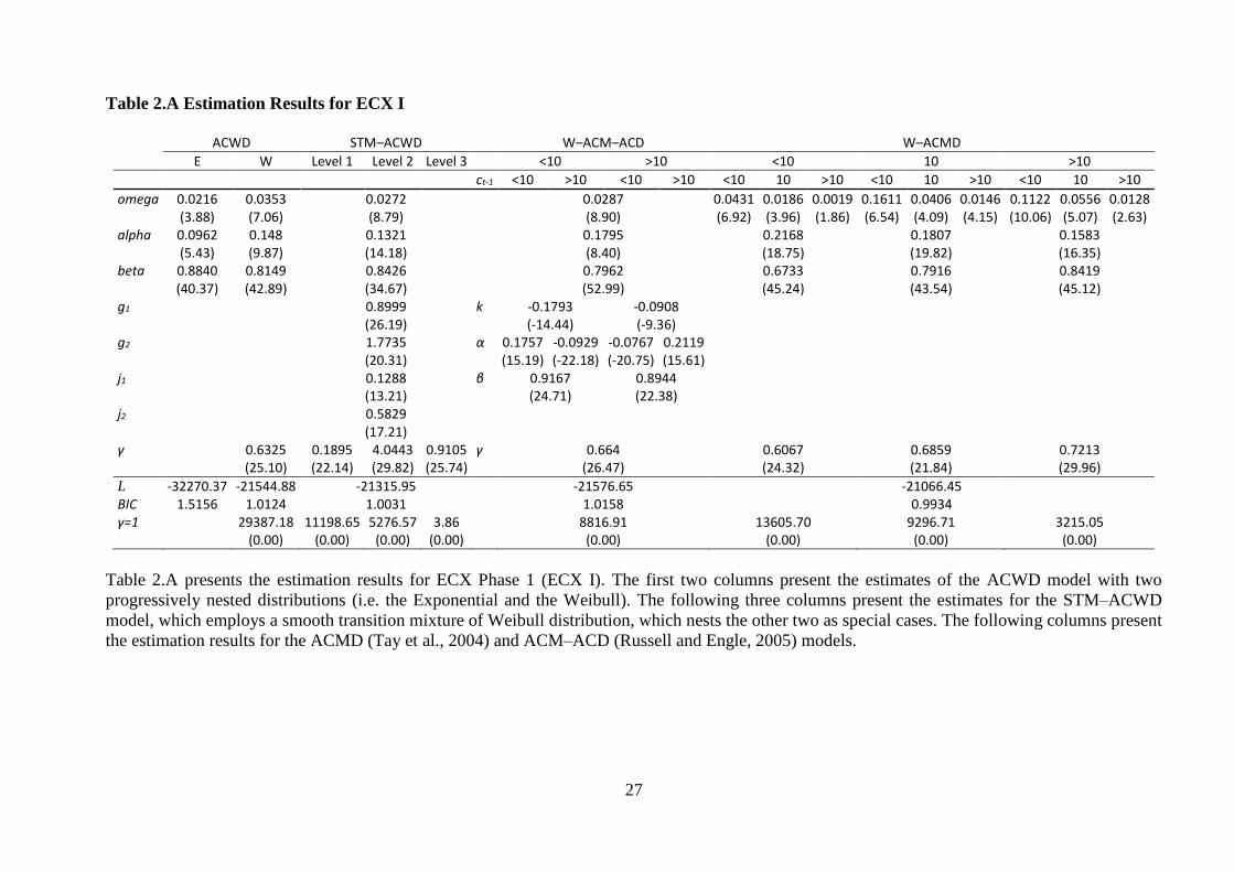
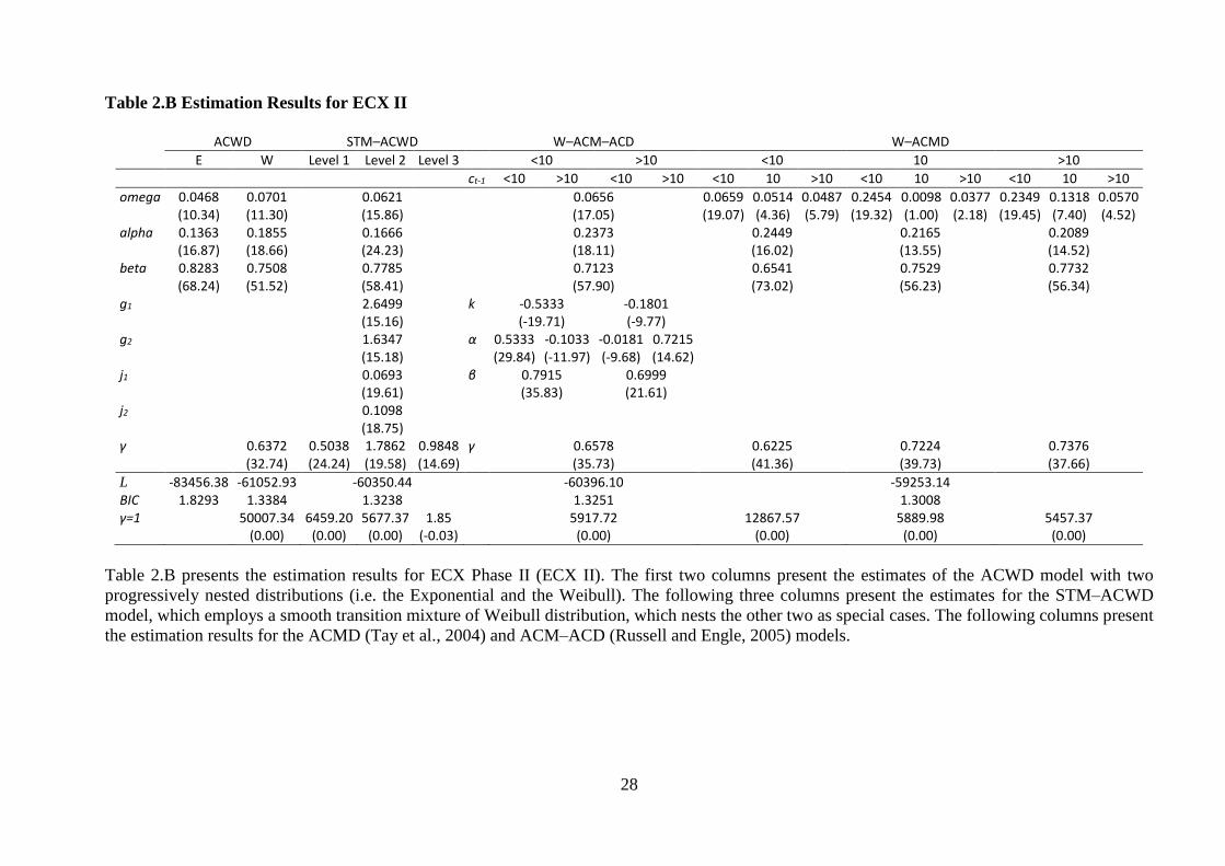
Estimation results of the ACWD model (equations 7, 8, 9 and 10) are presented in the first

five columns of Tables 2.A to 2.D. Almost all parameter estimates presented in the four tables

15 For the increasing levels of activity and market development, see, for example, IETA reports (2005–2009).

13

are statistically significant. In particular, estimates of alpha and beta for ACWD in all four

tables add up to less than, but close to, one. This indicates stationarity with high persistence,

underlying autoregressive dynamics, and hence the appropriateness of the ARMA/ACD

modelling framework, for trading intensity. Thus, intensity shocks have prolonged subsequent

effects, in the sense that a shock does not die out quickly, but persists over time.

The STM–ACWD model investigates persistence, separating the impact of different levels

or stages of trading intensity. The two threshold values j1 and j2 clarify the distribution of the

errors as a mixture of three Weibull distributions, and define high, medium and low levels of

trade intensity. Ji < j1 signals high trade intensity levels in the form of shorter weighted duration

per contract; j1 < Ji <j2 signals medium trade intensity levels or medium weighted duration per

contract; and Ji > j2 signals low trading intensity levels in the form of longer weighted duration

per contract. As discussed in Section 2.3, each of these three levels of trade intensity is

associated with a different Weibull distribution with a distinct shape parameter. These

parameters are γ1, γ2, and γ3 for high, medium and low intensity levels, respectively. Estimates

of the shape parameters are different from each other, confirming distinct levels or stages of

trade intensity. Estimates of γ1 for high levels of trading intensity are consistently less than one

(0.1895 in ECX I, 0.5038 in ECX II, 0.1954 in NP I and 0.2216 in NP II) implying a decreasing

hazard function for the arrival of subsequent contracts. In this regime the probability of a single

contract to be traded decreases over time and this means that when a large and/or fast trade is

observed in the market the arrival rate of contracts accelerates. In contrast, when a slow and/or

a small transaction is observed, as in the third level or stage of trading intensity, the estimate

of γ3 is always very close to one. This implies an almost flat hazard function, which means that

the arrival rate of a single contract is not expected to vary over time. Consequently, large and

fast trading seems to accelerate trading activity, whilst small and slow trading seems to be

prolonged.

These findings confirm the existence of the trading episodes identified by Kalaitzoglou and

Ibrahim (2013a). Easley and O’Hara (1992) and Engle (2000) argue that higher trading activity

is associated with the presence of price unresolved information and thus, is linked to higher

volatility. The decreasing hazard function following a high intensity trade indicates that trading

activity intensifies. This might create an episode, which is expected to end when a low trading

intensity shock, 𝜀𝑖, is observed, or when price relevant information is resolved. The volatility

impact of these trades is investigated in the next section.

The differential effect of each trade on the arrival rates of single contracts depends on the

threshold values j1 and j2, as well as on the smoothness parameters g1 and g2. Estimates of j1

14

are consistently relatively small (0.1288 in ECX I, 0.0693 in ECX II, 0.0896 in NP I and 0.0544

in NP II) compared to the theoretical mean of 1, which indicates a distinct group of trades with

relatively short duration per contract. They account for less than 30% of total trading in all

markets and phases. In contrast, the majority of trades, around 50%, lies beyond j2 (0.5829 in

ECX I, 0.1098 in ECX II, 0.1989 in NP I and 0.2469 in NP II). The degree of the transition

smoothness is captured by g1 and g2. Estimates of g1 are consistently less than those of g2 in

Phase I (0.8999<1.7735 in ECX and 1.1545<1.7727 in NP), but consistently larger in Phase II

(2.6499>1.6347 in ECX and 1.6524>1.1974 in NP). This indicates higher persistence of trading

intensity following a large and/or fast trade in Phase I, which seems to return to a ‘normal’

stage, i.e. beyond j2, faster than it goes from a high to a middle trading intensity stage. In

contrast, in Phase II, the high trading intensity episodes seem to be faster resolved into middle

stage trading intensity, while the transition from middle to low is rather stable. Kalaitzoglou

and Ibrahim (2013b) relate this to greater market depth and market maturity in Phase II. In

Section 4.3 we investigate this further by measuring uncertainty resolution in calendar time.

Faster resolution would indicate greater maturity.

Furthermore, the above empirical findings are visually presented and confirmed in Figure

2. When trading intensity is below j1, i.e. high trading activity, the probability density function

(PDF) is sharply decreasing with an associated decreasing hazard function. Trading, therefore,

is expected to continue being intense. In contrast, when trading intensity is around j2, the

process seems to be reverting. When trading intensity is below j2, the PDF is bell-shaped

indicating a higher probability of smaller and/or slower trading. When trading intensity is

above j2, the density is still bell–shaped but closer to the Exponential distribution. This

indicates a closer proximity to a flat hazard function and hence, more non–high–trading–

intensity trades.

These findings are confirmed by the estimation of the two alternative discrete models,

namely the ACMD and the ACM–ACD. For both of these latter models we use three states of

the associated mark, the choice of which is guided by the unconditional basic statistics. The

median volume is about 10 contracts, and this is defined as one state. The other two states

consist of trades associated with less or more than 10 contracts, respectively. For consistency

the Weibull distribution is employed. The ACM–ACD approach models the transition

probabilities as time varying functions as in Equation 15 in the Appendix. The parameter

matrices of interest are A and B, which indicate the structure of the transition matrix. Estimates

of β (elements of B) are consistently high (e.g., 0.9167 and 0.8944 in ECX I) showing high

persistence in volume continuation, i.e. the probability of a small (large) trade to follow a small

15

(large) one. This is confirmed by α’s (elements of A) where the probability of volume

continuation (e.g., 0.2057 – a small trade follows a small trade – and 0.1759 – a large trade

follows a large trade – in NP I) is higher than the probability of a reversal (e.g., -0.0870 – a

small trade follows a large trade – and -0.0646 – a large trade follows a small trade – in NP I).

This is also consistent with the estimation results of the ACMD (Equation 11 in the Appendix)

where the transition probabilities are captured by the dissected intercept, 𝜔𝑐, of the three

competing processes. Average duration is consistently shorter after a large trade (e.g., 0.0487,

0.0377 and 0.0570 in ECX II), and consistently longer after a small trade (e.g., 0.0659, 0.2454

and 0.3249 in ECX II). Consequently, all three models highlight that liquidity is persistent, in

the sense that high trading intensity trades tend to be followed by larger and/or faster trades.

Although the benchmark ACMD and the ACM–ACD models show the consistency of the

ACWD in identifying the persistence of liquidity, there is a fundamental difference. These

benchmark models require the states to be pre–specified, and persistence is shown above to be

consistent with the chosen volume states of >10, 10 and <10 contracts. The possibility of mis–

specifying the states would, therefore, be a potential source of error. In contrast, the ACWD

model has no need to identify states of the mark (volume), since the mark and duration are

combined in one variable. In addition, the smooth transition mechanism (STM) feature of the

STM–ACWD, with the two threshold values j1 and j2 (which are estimated jointly with the

model), identifies relative levels of this new liquidity measure (trading intensity), while the

ACMD and ACM–ACD specifications lack this feature.

Another main result relates to the modelling approach, as well as the level of generality of

the associated distribution required in order to take into account necessary features of the data’s

higher moments, especially the joint distribution of durations and volume. In Table 3 we

compare the performance of the models based on their in-sample fit and out-of-sample forecast

accuracy. The values of Q–stat(15) are mostly insignificant for the ACWD models, ranking

them as the best fitting models, especially the versions with the mixture of Weibull

distributions. This indicates that the linear ACWD framework captures autocorrelation in both

markets and both phases, and that the (1,1) lag structure is a parsimonious specification.

However, for the ACMD and ACM–ACD models the reported significant Q–statistics indicate

that some autocorrelation remains unaccounted for, or induced by the discrete character of

these models. Further, increased flexibility of the density functions is rewarded with better

ranking. The smooth transition mixture of Weibull distributions performs better than the

Weibull (W), which in turn performs better than the Exponential (E). More importantly, the

maximum log-likelihood function value (L) is significantly (statistically) greater for the model

16

estimated with the mixture of Weibull distribution than with the Weibull or the Exponential, in

this order.16 Moreover, we use two measures to test relative forecast performance: the Unitised

Loss (UNL), which is the average squared forecast error per unit of forecast value, and the

correlation (CORR) between actual and forecasted values (see the ‘Performance’ section in the

Appendix for more detail). According to these measures the ACMD is the worst of the three

models, while the STM–ACWD is the best. These rankings suggest that the volume weighted

duration modelling with the joint distribution better captures the data generation process of

trading intensity, i.e. duration and volume, than the discrete marks approach. This is consistent

across both in–sample and out–of–sample 1–step forecasts (see Appendix for more detail on

forecasting setup).

In contrast, the 10–step out–of–sample forecasts show that simpler density specifications

should be preferred. These findings show that dependence on trading activity dynamics are

more important for short term investment horizons, where higher complexity and/or flexibility,

i.e. more flexible conditional density, are rewarded with higher forecasting accuracy. In

contrast, trading activity seems to be less dependent on trading intensity persistence in the long

term, and appears to converge to general long–term market dynamics, which are expected to

follow macroeconomic fundamentals. Therefore, more parsimonious linear specifications tend

to provide more accurate forecasts in the relatively longer term. This, again, highlights the

differences between relative and absolute liquidity. Higher relative liquidity appears to create

high trading intensity episodes, and that is why more complex distributions are better able to

explain short–term dynamics. However, in the longer term the resolution of these episodes

depends more on general market conditions, and thus on absolute rather than on relative

liquidity. Therefore, the explanatory power of more complex distributions, which are more

sensitive to trading intensity persistence, is dependent on relative market conditions.

4.3 Intraday Uncertainty Resolution

16 The nesting property of the STM mixture of Weibull distribution to the Weibull and the Exponential

distributions facilitates testing by the Likelihood Ratio (LR). For example, in Table 2.A the ACWD Log–

likelihood function values, L, are -21544.88 for a Weibull distribution and -21315.5 for the STM, giving a LR test

statistic of 458.76, which is far larger than the 5% critical value of 12.59. This indicates that the ACWD model

with the STM distribution is significantly better than with the Weibull distribution (both statistically and in terms

of likelihood). Strictly speaking, the LR test cannot be used to test whether the ACWD fits better than the discrete

mark models because these models are not nested.

17

Previous literature associates these liquidity episodes with increased price change volatility

(e.g., Kalaitzoglou and Ibrahim, 2013a). Trades characterised by higher relative liquidity have

been implicitly reported to be associated with a higher presence of price unresolved

information. In this paper, we accept that they might indeed convey price related information

signals that are not yet reflected into price changes, and therefore trigger a high trading intensity

episode. However, we investigate further cases where there might not be a general market

consensus about the magnitude and the direction of the information. This, especially when

private or imperfect public information and increased ambiguity co–exist, should introduce

uncertainty in the form of increased volatility. More efficient market environments should

incorporate information faster and, thus, shorten the duration of these episodes. We investigate

whether higher absolute liquidity contributes to faster uncertainty resolution. Specifically, we

focus on potential uncertainty induced by higher relative liquidity trades and investigate how

different market environments absorb the shock. The main interest lies in the magnitude of the

impact, on how long it takes for price change volatility to return to normal levels and how this

changes over the trading day and across markets and phases.

Figure 3 presents the average price change volatility for the five transactions that precede

and the twenty that follow a high intensity trade (Ji <j1), at every hour of the trading day.

Motivated by the microstructure literature that investigates the permanent and temporary price

impact of trades (see e.g., Frino et al., 2010) we consider the prior five transactions as the

‘current’ state of the market, while the length of the following window (twenty trades) is chosen

according to the maximum length of impact found in our data. Beyond twenty transactions

almost all effects of relative high intensity trades fade out. The first major finding from Figure

3 is that notably higher volatility is observed for a time period following the appearance of high

intensity trades. However, this volatility shock is not very sharp in magnitude and seems to be

rather prolonged. This is a sign that higher relative liquidity is indeed perceived to carry price

unresolved information, leading to increased volatility. However, there is no sharp price change

that rapidly incorporates this piece of information into prices. Instead, depending on the time

of day, a period of increased, or high and decreasing, volatility is observed when prices are

gradually adjusted. Consequently, and in accordance with O’Hara (2003), information

resolution is observed to be a gradual partially revealing process, rather than an instantaneous

event. This prolonged uncertainty might create exploitable market frictions, which might attract

increased trading. This is probably the reason why high trading intensity episodes seem to be

prolonged, at least until price relevant information is resolved.

18

In addition, the average magnitude of the volatility impact of high trading intensity trades

increases over the trading day, exhibiting the highest spikes towards the closing of the market.

This is somewhat expected because the overall trading activity and the number of high trading

intensity trades increases after the lunch break (see Figure 4) and less information resolution is

expected towards the end of the trading sessions (Roll, 1984). Consequently, an unexpectedly

large trade should be more distinct and more clearly linked to excessive information and hence

it appears to have a higher price impact.

Finally, Figure 5 presents the product of average duration during a high trading intensity

episode and the number of transactions it takes for price change volatility to return to its prior

‘normal’ level.17 This product measures, in minutes, the time it takes each market environment

to absorb high trading intensity volatility shocks, and how this changes over the trading day.

From Figure 5, the informational content of high trading intensity trades needs at least 7.65

minutes (ECX II) to be resolved. Values of this measure vary over the trading day and across

markets and phases ranging from 7.65 at the opening of the ECX II market, to more than 2

hours during lunch break in NP II. Phase I in both markets is less liquid, and certain events

affect trading activity more than in Phase II, while their effect seems to last longer. This is an

indication of increased sensitivity to absolute liquidity or insufficient market depth, where

certain events are noticeable. As market gradually gains liquidity towards Phase II these events

have a lower volatility impact and are absorbed more smoothly and faster, which is interpreted

as a more mature trading environment. Overall, the uncertainty resolution time is considerably

shorter in ECX, especially in Phase II. This confirms that absolute liquidity is an important

factor for uncertainty resolution, with ECX clearly leading, at least time wise, the intraday price

discovery.

In addition, the uncertainty resolution time consistently increases in all markets and phases

until lunch break. This shows that there is accumulated overnight information that is resolved

faster during the opening of the market because liquidity is higher and market participants

appear to be more sensitive to high trading intensity shocks. After lunch break, however, the

uncertainty resolution time decreases again, especially in NP. Following NP market close, the

time length of uncertainty resolution in ECX drops drastically, especially in Phase I. This

highlights the importance of the overlapping period, which seems to allow for information

17 We define as ‘normal’ the average price change volatility of the last five transactions prior to the appearance of

a high trading intensity trade (Ji<j1). We then measure the number of transactions till subsequent price change

volatility decreases for the first time below this ‘normal’ level. We repeat the process for every hour interval.

19

exchange or perhaps a cross–market liquidity influence.18 The flow of trades between the

organised markets seems to prolong the uncertainty resolution time, probably due to increased

ambiguity concerning the informational content of incoming trades. This indicates that,

although ECX is markedly more liquid, NP also significantly contributes to intraday price

discovery during the overlapping period, in the sense that investors seem to take into

consideration that information and liquidity might flow from one market to the other. This is

consistent with Benz and Hengelbrock (2008) who measure the informational share of both

ECX and NP and indicate the leadership of ECX in intraday price discovery.

Consequently, this analysis highlights a major difference between two distinct aspects of

liquidity. Absolute liquidity, defined as the overall volume of trading, improves market

efficiency, in the sense of lower in magnitude volatility shocks and faster uncertainty

resolution. This might be related to lower execution risks or greater number of noise traders

that allows dealers to recover potential losses by trading with better informed agents easier. In

contrast, relative liquidity, defined as greater trading intensity compared to previous trades, is

linked to price unresolved information and, thus, introduces uncertainty.

This is further confirmed by the fitting of the models, where the more sophisticated

continuous ACWD specifications fit and forecast better in the short–term (1–step forecasts),

while more parsimonious specifications are predominant in the long term (10–step forecasts).

This indicates that trading momentums at intra-day level, which might induce liquidity or

volatility shocks, are significant within a short time period, in which investors can extract and

exploit temporal information advantages or arbitrage opportunities. In contrast, the temporal

dependence of trading activity over longer time periods seems weaker, suggesting that it is

driven more by exogenous stimuli, rather than by trading history. This difference highlights

that there exists a time period when market frictions, such as relatively high trading intensity

trades, could create exploitable opportunities due to increased ambiguity. However, when

absolute liquidity increases, price liquidity is faster and therefore, potential market frictions are

exploitable for a shorter period of time. This is a sign of higher levels of market efficiency.

5. Summary and Conclusion

We propose volume weighed durations as a direct measure of trading intensity. We model

the dynamic structure of this temporal marked point process (t.m.p.p) as a rescaled temporal

18 The ACWD framework, therefore, may be useful in studying cross–market or cross–asset liquidity. We thank

an anonymous referee for bringing this point to our attention.

20

point process (t.p.p), weighted on the magnitude of the associated mark of interest. This

provides a measure of the waiting time per unit of the associated mark. Consequently, we

measure trading intensity as the waiting time of a single contract. This is a notable improvement

over existing models, which model t.m.p.p’s assuming discrete state marks. The new

framework, named Autoregressive Conditional Weighted Duration (ACWD), relaxes this

assumption and is found to significantly outperform two existing models; the ACM–ACD

model by Russell and Engle (2005) and the ACMD model by Tay et al. (2004).

Furthermore, we employ a specification similar to Kalaitzoglou and Ibrahim (2013b) to

identify different regimes of trading intensity in the European Carbon Futures market. We

investigate whether distinctively high trading intensity trades introduce uncertainty by

measuring their volatility impact. Then, the uncertainty resolution period is measured in

calendar time, in the two largest exchanges of EU ETS, which differ substantially in overall

liquidity. With this set up we propose a first time explicit distinction between two different

types of liquidity, “absolute” or overall liquidity, which measures overall market activity, and

“relative” liquidity, which measures relative market activity with respect to a benchmark, e.g.

compared to average or absolute liquidity.

Higher relative liquidity is found to introduce uncertainty, which is translated into higher

price change volatility. The increased volatility does not “die out” immediately; it needs some

resolution time. Uncertainty resolution times seem to be increasing from market opening until

lunch break when they start decreasing. They drop drastically after the closing of NP, which

indicates that price discovery takes place in both markets. This process is markedly faster in

more liquid environments, such as the ECX, especially in Phase II. This indicates a dual role

for liquidity; higher relative liquidity introduces uncertainty, while higher absolute liquidity

improves market maturity by accelerating uncertainty resolution time.

21

Appendix

Discrete State Modelling

ACWD is tested against the following specifications:

W–ACMD

𝜓𝑖,𝑐 = 𝜔𝑐 ∑ 𝐷𝑐,𝑖−13𝑐=1 + 𝑎𝑐𝑥𝑖−1 + 𝛽𝑐𝜓𝑖−1, (11)

𝑓 ((𝑥𝑖

𝜓𝑖,𝑐)| ; 𝜏𝐴𝐶𝑀𝐷) = (γ

𝑐𝑥𝑖⁄ )[𝑥𝑖𝛤(1 + 1 γ

𝑐⁄ ) 𝜓𝑖,𝑐⁄ ]

γ𝑐exp (−[𝑥𝑖𝛤(1 + 1 γ𝑐

⁄ ) 𝜓𝑖,𝑐⁄ ]γ𝑐) (12)

W–ACM–ACD

𝜓𝑖 = 𝜔 + α𝜀𝑖−1 + 𝛽𝜓𝑖−1, (13)

𝑓 ((𝑥𝑖

𝜓𝑖)| ; 𝜏𝐴𝐶𝑀−𝐴𝐶𝐷) = (𝛾 𝑥𝑖⁄ )[𝑥𝑖𝛤(1 + 1 𝛾⁄ ) 𝜓𝑖⁄ ]γ exp(−[𝑥𝑖𝛤(1 + 1 𝛾⁄ ) 𝜓𝑖⁄ ]𝛾), (14)

ℎ(𝜋𝑖) = 𝐾 + 𝐴(𝑐𝑖−1 − 𝜋𝑖−1) + 𝐵ℎ(𝜋𝑖−1), (15)

where, 𝜀𝑖 = 𝑥𝑖 𝜓𝑖⁄ , x is realised diurnally–adjusted duration, ψ is its expected value, γ is the

shape parameter of a Weibull distribution, and 𝐷𝑐,𝑖 is a dummy variable that takes the value of

1 when the associate mark of a trade i is in state c, and zero otherwise. Based on unconditional

descriptive statistics we consider three states (c) of volume: <10, 10 and >10 contracts. For the

ACM model, 𝜋𝑖 is the probability of the state of the associated mark, conditional on past

information, and ℎ(·) is the inverse logistic function formulated in Equation 15 conditional on

its past values and state probability. 𝜏𝐴𝐶𝑀𝐷 = (𝜔𝑐, 𝑎𝑐, 𝛽𝑐, γ𝑐) and 𝜏𝐴𝐶𝑀−𝐴𝐶𝐷 =

(𝜔, α, 𝛽, 𝛾, 𝐾, 𝐴, 𝐵) are vectors of parameters, with 𝐴 = (𝛼11 𝛼13

𝛼31 𝛼33), 𝐵 = (

𝛽1 00 𝛽3

) and 𝐾 =

(𝑘1 𝑘3)′.

One Step Forecasts

‘Short–term’ (1–step) forecasts are generated according to the conditional mean specifications.

We assume that the expected value of the associated mark of each state 𝐸𝑐,𝑖(𝜐𝑖+1) equals the

unconditional expectation 𝐸𝑐(𝜐) in this state over the sample period. For the ACMD model we

assume that the shortest duration defines the winning state (Kwok et al., 2009). The 1–step

forecasts are 𝐸𝑖,𝐴𝐶𝑀𝐷 [𝑥𝑖+1

𝜐𝑖+1] = [

𝜓𝑐,𝑖+1

𝐸𝑐,𝑖(𝜐𝑖+1)] = [

min (𝜓𝑐,𝜄+1)

𝐸(𝑐| min(𝜓𝑐,𝜄+1))(𝜐)] for the ACMD, while for the

ACM–ACD are 𝐸𝑖,𝐴𝐶𝑀−𝐴𝐶𝐷 [𝑥𝑖+1

𝜐𝑖+1] = [

𝜓𝑖+1

𝐸𝑐,𝑖(𝜐𝑖+1)] = 𝐸𝑖 [

𝜓𝜄+1

∑ 𝜋𝑖+1𝐸𝑐(𝜐)3𝑐=1

], where 𝜋𝑖 =

exp (𝐾+𝐴(𝑐𝑖−1−𝜋𝑖−1)+𝐵ℎ(𝜋𝑖−1))

1+𝑖′exp (𝐾+𝐴(𝑐𝑖−1−𝜋𝑖−1)+𝐵ℎ(𝜋𝑖−1)) and i′ is a conforming vector.

S Step Forecasts

22

Following Dufour and Engle (2000) s-term forecasts for the ACWD are given by 𝐸𝑖[𝑆𝑖+𝑠] =

𝜔1−(𝛼+𝛽)𝑠−1

1−(𝛼+𝛽)+ (𝛼 + 𝛽)𝑠−1𝛩𝜄+1. Likewise, the s-step forecasts for ACMD are given by

𝐸𝑖,𝐴𝐶𝑀𝐷 [𝑥𝑖+𝑠

𝜐𝑖+𝑠

] = [𝜓𝑐,𝑖+𝑠

𝐸𝑐,𝑖(𝜐𝑖+𝑠)] = [

min (𝜓𝑐,𝜄+𝑠)

𝐸(𝑐| min(𝜓𝑐,𝜄+𝑠))(𝜐)] =

𝑚𝑖𝑛((𝜔𝑐 ∑ 𝐷𝑐,𝑖3𝑐=1 )

1−(𝑎𝑐+𝛽𝑐)𝑠−1

1−(𝑎𝑐+𝛽𝑐)+(𝑎𝑐+𝛽𝑐)𝑠−1𝜓𝜄+1)

𝐸(𝑐| min(𝜓𝑐,𝜄+𝑠))(𝜐).

For ACM–ACD the s-step forecasts are given by 𝐸𝑖,𝐴𝐶𝑀−𝐴𝐶𝐷 [𝑥𝑖+𝑠

𝜐𝑖+𝑠

] = [𝜓𝑖+𝑠

𝐸𝑐,𝑖(𝜐𝑖+𝑠)] =

[𝜓𝜄+𝑠

∑ 𝜋𝑖+𝑠𝐸𝑐(𝜐)3𝑐=1

], where 𝜓𝜄+𝑠 = 𝜔1−(𝛼+𝛽)𝑠−1

1−(𝛼+𝛽)+ (𝛼 + 𝛽)𝑠−1𝜓𝜄+1 and 𝜋𝑖+𝑠 =

exp (𝐾1−(𝐴+𝐵)𝑠−1

1−(𝐴+𝐵)+(𝐴+𝐵)𝑠−1ℎ(𝜋𝜄+1))

1+𝑖;exp (𝐾1−(𝐴+𝐵)𝑠−1

1−(𝐴+𝐵)+(𝐴+𝐵)𝑠−1ℎ(𝜋𝜄+1))

.

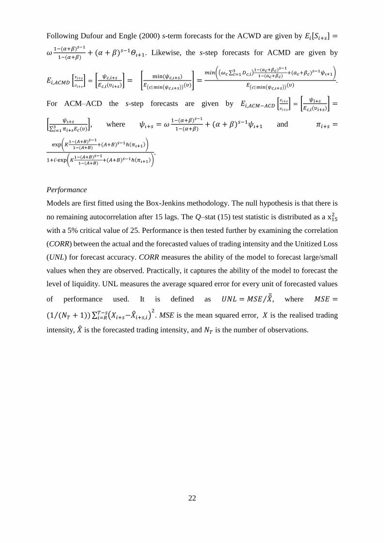
Performance

Models are first fitted using the Box-Jenkins methodology. The null hypothesis is that there is

no remaining autocorrelation after 15 lags. The Q–stat (15) test statistic is distributed as a x152

with a 5% critical value of 25. Performance is then tested further by examining the correlation

(CORR) between the actual and the forecasted values of trading intensity and the Unitized Loss

(UNL) for forecast accuracy. CORR measures the ability of the model to forecast large/small

values when they are observed. Practically, it captures the ability of the model to forecast the

level of liquidity. UNL measures the average squared error for every unit of forecasted values

of performance used. It is defined as 𝑈𝑁𝐿 = 𝑀𝑆𝐸 ��⁄ , where 𝑀𝑆𝐸 =

(1 (𝑁𝑇 + 1)⁄ ) ∑ (𝑋𝑖+𝑠−��𝑖+𝑠,𝑖)2𝑇−𝑠

𝑖=𝑅 . MSE is the mean squared error, 𝑋 is the realised trading

intensity, �� is the forecasted trading intensity, and 𝑁𝑇 is the number of observations.

23

References

Alberola, E., Chevallier, J. and Chèze, B. (2008) Price drivers and structural breaks in European

carbon prices 2005-07. Energy Policy 36:787-797.

Amihud, Y. and Mendelson, H. (1980) Dealership market. Market–making with Inventory.

Journal of Financial Economics 8, 31–53.

Bagehot, W. (1971) The only game in town. Financial Analysts Journal 27(2), 12–14.

Benston, G. J. and Hagerman, R. L. (1974) Determinants of bid-asked spreads in the over-the-

counter market. Journal of Financial Economics, 1(4), 353–364.

Benz, E. A. and Hengelbrock, J. (2008) Price discovery and liquidity in the European CO2

futures market: An intraday analysis. Unpublished manuscript, Bonn Graduate School of

Economics. Available at http://ssrn.com/abstract=1131770.

Bredin, D., Hyde, S. and Muckley, C. (2014) A microstructure analysis of the carbon finance

market. International Review of Financial Analysis. Available online, doi:

10.1016/j.irfa.2014.03.003.

Cappor, K. and Ambrosi, P. (2006–2009) State and trends of the carbon market. World Bank

Washington, DC.

Cohen, K. J., Hawawini, G. A., Maier, S. F., Schwartz, R. A. and Whitcomb, D. K. (1980)

Implications of microstructure theory for empirical research on stock price behavior.

Journal of Finance 35(2), 249–257.

Cohen, K. J., Maier, S. F., Schwartz, R. A. and Whitcomb, D. K. (1981) Transaction costs,

order placement strategy, and existence of the bid-ask spread. The Journal of Political

Economy 89(2), 287–305.

Convery F. J. and Redmond L. (2007) Market and price developments in the European Union

Emissions Trading Scheme. Review of Environmental Economics and Policy 1(1), 88–111.

Daley, D. J. and Vere-Jones, D. (2003) An introduction to the theory of point processes. In

Elementary theory and methods of probability and its applications, Volume 1. Springer,

New York.

Daskalakis, G., Psychoyios, D. and Markellos, R. N. (2009) Modeling CO2 emission allowance

prices and derivatives: Evidence from the European trading scheme. Journal of Banking

& Finance 33(7), 1230–1241.

Dufour, A. and Engle, R. F. (2000) Time and the price impact of a trade. The Journal of Finance

55, 2467–2498.

Easley, D. and O’Hara, M. (2010) Microstructure and ambiguity. The Journal of Finance 65(5),

1817–1846.

http://dx.doi.org/10.1016/j.irfa.2014.03.003

http://dx.doi.org/10.1016/j.irfa.2014.03.003

24

Easley, D. and O'Hara, M. (1992) Time and the process of security price adjustment. Journal

of Finance 47(2), 577–605.

Engle, R. F. (2000) The econometrics of ultra–high–frequency data. Econometrica 68(1), 1–

22.

Engle, R. F. and Russell, J. R. (1998) Autoregressive conditional duration: A new model for

irregularly spaced transaction data. Econometrica 66(5), 1127–1162.

Epanechnikov, V. A. (1969) Non–parametric estimation of a multivariate probability density.

Theory of Probability and its Applications 14, 153–158.

Frino, A., Kruk, J., and Lepone, A. (2010) Liquidity and transaction costs in the European

carbon futures market. Journal of Derivatives and Hedge Funds 16, 100–115.

Garman, M. B. (1976) Market microstructure. Journal of Financial Economics 3(3), 257–275.

Glosten, L. and Milgrom, P. (1985) Bid, ask and transactions prices in a specialist market with

insider trading. Journal of Financial Economics 14, 71–100.

Grossman, S. J. and Miller, M. H. (1988) Liquidity and market structure. Journal of Finance

43, 617–633.

Hayek, F. A. (1945) The use of knowledge in society. The American Economic Review 4, 519–

530.

Ho, T. S. Y. and Stoll, H. (1981) Optimal dealer pricing under transactions and return

uncertainty. Journal of Financial Economics 9, 47–73.

Ho, T. S. Y. and Stoll, H. R. (1983) The dynamics of dealer markets under competition. Journal

of Finance 38(4), 1053–1074.

Ibikunle, G., Gregoriou, A. and Pandit, N. (2011) Liquidity effects on carbon financial

instruments in the EU emissions trading scheme: New evidence from the Kyoto

commitment phase. Working paper, University of Edinburgh.

International Emissions Trading Association (IETA) Annual Report (2005-2009). Available at

http://www.ieta.org/reports.

Kalaitzoglou, I. and Ibrahim, B. M. (2013a) Trading patterns in the European carbon market:

The role of trading intensity and OTC transactions. The Quarterly Review of Economics

and Finance 53(4), 402–416.

Kalaitzoglou, I. and Ibrahim, B. M. (2013b) Does order flow in the European carbon futures

market reveal information? Journal of Financial Markets 16(3), 604–635.

Kwok, S. S. M., Li, W. K. and Yu, P. L. H. (2009) The autoregressive conditional market

duration model: Statistical inference to market microstructure. Journal of Data Science 7,

189–201.

25

Kyle, A. S. (1985) Continuous auctions and insider trading. Econometrica 53(6), 1315–1335.

Kyle, A. S. and Viswanathan, S. (2008) How to define illegal price manipulation. The

American Economic Review 98(2), 274–279.

Madhavan, A., Richardson, M. and Roomans, M. (1997) Why do security prices change? A

transaction–level analysis of NYSE stocks. Review of Financial Studies 10(4), 1035–1064.

Mansanet-Bataller, M. and Pardo, A. (2008) What you should know about carbon markets.

Energies 1(3), 120–153.

Mizrach, B. and Otsubo, Y. (2014) The market microstructure of the European Climate

Exchange. Journal of Banking & Finance 39(2), 107–116.

O'Hara, M. (2003) Presidential address: Liquidity and price discovery. The Journal of Finance

58(4), 1335–1354.

O'Hara, M. (2011) Market microstructure theory. Blackwell Publishing, Oxford, UK.

Ranaldo, A. (2001) Intraday market liquidity on the Swiss stock exchange. Financial Markets

and Portfolio Management 15(3), 309–327.

Roll, R. (1984) A simple implicit measure of the effective bid-ask spread in an efficient market.

Journal of Finance 39, 1127–1139.

Russell, J. R. (1999) Econometric modelling of multivariate irregularly-spaced high-frequency

data. Working paper. University of Chicago.

Russell, J. R. and Engle, R. F. (2005) A discrete–state continuous–time model of financial

transactions prices and times. Journal of Business & Economic Statistics 23(2), 166–180.

Sarr, A. and Lybek, T. (2002) Measuring liquidity in financial markets. IMF Working Paper,

WP/02/232.

Stoll, H. R. (1978) The pricing of security dealer services: An empirical study of NASDAQ

stocks. Journal of Finance 33(4), 1153–1172.

Tay, A. S, Ting, C., Tse, Y.K. and Warachka, M. (2004) Transaction–data analysis of marked

durations and their implications for market microstructure. Working paper. Singapore

Management University, School of Economics.

Tinic, S. M. and West, R. (1972) Competition and the pricing of dealer service in the over–

the–counter stock market. Journal of Financial and Quantitative Analysis 7(3), 1707–

1728.

Tinic, S. M. (1972) The economics of liquidity services. The Quarterly Journal of Economics

86(1), 79–93.

Viswanathan, S. (2010). Developing an efficient carbon emissions allowance market. Working

paper. Duke University, Fuqua School of Business.

26

Table 1. Descriptive Statistics

ECX I ECX II NP I NP II

Duration Volume Price Duration Volume Price Duration Volume Price Duration Volume Price Mean 375.87 12.45 19.85 75.73 9.69 22.6 1912.21 10.81 20.33 1370.57 10.67 22.73

Median 79 10 20.41 23 5 22.85 480 10 21.27 540 10 22.92 Maximum 30979 500 33.72 4332 500 32.35 29933 250 33.5 20542 308 37.25 Minimum 1 1 10.75 1 1 11.16 1 1 12.01 1 1 11.56 Std. Dev. 1264.10 18.16 2.97 157.15 19.4 3.33 3727.12 11.77 2.99 2195.64 14.51 2.79 Skewness 11 10.93 -0.37 7.29 11.02 -0.41 3.71 7.07 -0.64 3.28 9.28 -0.35 Kurtosis 168.44 216.24 2.74 109.26 198.51 2.65 19.69 92.87 2.78 17.63 130.03 4.47

Table 1 presents descriptive statistics for raw duration (in seconds), volume and price. ECX is the European Climate Exchange, NP is the Nord Pool

Exchange and the suffix I or II refer to Phase I sample (2006-2007) and Phase II sample (2008).

27

Table 2.A Estimation Results for ECX I

ACWD STM–ACWD W–ACM–ACD W–ACMD

E W Level 1 Level 2 Level 3 <10 >10 <10 10 >10

ct-1 <10 >10 <10 >10 <10 10 >10 <10 10 >10 <10 10 >10

omega 0.0216 0.0353 0.0272 0.0287 0.0431 0.0186 0.0019 0.1611 0.0406 0.0146 0.1122 0.0556 0.0128 (3.88) (7.06) (8.79) (8.90) (6.92) (3.96) (1.86) (6.54) (4.09) (4.15) (10.06) (5.07) (2.63) alpha 0.0962 0.148 0.1321 0.1795 0.2168 0.1807 0.1583 (5.43) (9.87) (14.18) (8.40) (18.75) (19.82) (16.35) beta 0.8840 0.8149 0.8426 0.7962 0.6733 0.7916 0.8419 (40.37) (42.89) (34.67) (52.99) (45.24) (43.54) (45.12) g1 0.8999 k -0.1793 -0.0908 (26.19) (-14.44) (-9.36) g2 1.7735 α 0.1757 -0.0929 -0.0767 0.2119 (20.31) (15.19) (-22.18) (-20.75) (15.61) j1 0.1288 β 0.9167 0.8944 (13.21) (24.71) (22.38) j2 0.5829 (17.21) γ 0.6325 0.1895 4.0443 0.9105 γ 0.664 0.6067 0.6859 0.7213 (25.10) (22.14) (29.82) (25.74) (26.47) (24.32) (21.84) (29.96)

L -32270.37 -21544.88 -21315.95 -21576.65 -21066.45 BIC 1.5156 1.0124 1.0031 1.0158 0.9934 γ=1 29387.18 11198.65 5276.57 3.86 8816.91 13605.70 9296.71 3215.05 (0.00) (0.00) (0.00) (0.00) (0.00) (0.00) (0.00) (0.00)

Table 2.A presents the estimation results for ECX Phase 1 (ECX I). The first two columns present the estimates of the ACWD model with two

progressively nested distributions (i.e. the Exponential and the Weibull). The following three columns present the estimates for the STM–ACWD

model, which employs a smooth transition mixture of Weibull distribution, which nests the other two as special cases. The following columns present

the estimation results for the ACMD (Tay et al., 2004) and ACM–ACD (Russell and Engle, 2005) models.

28

Table 2.B Estimation Results for ECX II



ct-1 <10 >10 <10 >10 <10 10 >10 <10 10 >10 <10 10 >10

omega 0.0468 0.0701 0.0621 0.0656 0.0659 0.0514 0.0487 0.2454 0.0098 0.0377 0.2349 0.1318 0.0570 (10.34) (11.30) (15.86) (17.05) (19.07) (4.36) (5.79) (19.32) (1.00) (2.18) (19.45) (7.40) (4.52) alpha 0.1363 0.1855 0.1666 0.2373 0.2449 0.2165 0.2089 (16.87) (18.66) (24.23) (18.11) (16.02) (13.55) (14.52) beta 0.8283 0.7508 0.7785 0.7123 0.6541 0.7529 0.7732 (68.24) (51.52) (58.41) (57.90) (73.02) (56.23) (56.34) g1 2.6499 k -0.5333 -0.1801 (15.16) (-19.71) (-9.77) g2 1.6347 α 0.5333 -0.1033 -0.0181 0.7215 (15.18) (29.84) (-11.97) (-9.68) (14.62) j1 0.0693 β 0.7915 0.6999 (19.61) (35.83) (21.61) j2 0.1098 (18.75) γ 0.6372 0.5038 1.7862 0.9848 γ 0.6578 0.6225 0.7224 0.7376 (32.74) (24.24) (19.58) (14.69) (35.73) (41.36) (39.73) (37.66)

L -83456.38 -61052.93 -60350.44 -60396.10 -59253.14 BIC 1.8293 1.3384 1.3238 1.3251 1.3008 γ=1 50007.34 6459.20 5677.37 1.85 5917.72 12867.57 5889.98 5457.37 (0.00) (0.00) (0.00) (-0.03) (0.00) (0.00) (0.00) (0.00)

Table 2.B presents the estimation results for ECX Phase II (ECX II). The first two columns present the estimates of the ACWD model with two




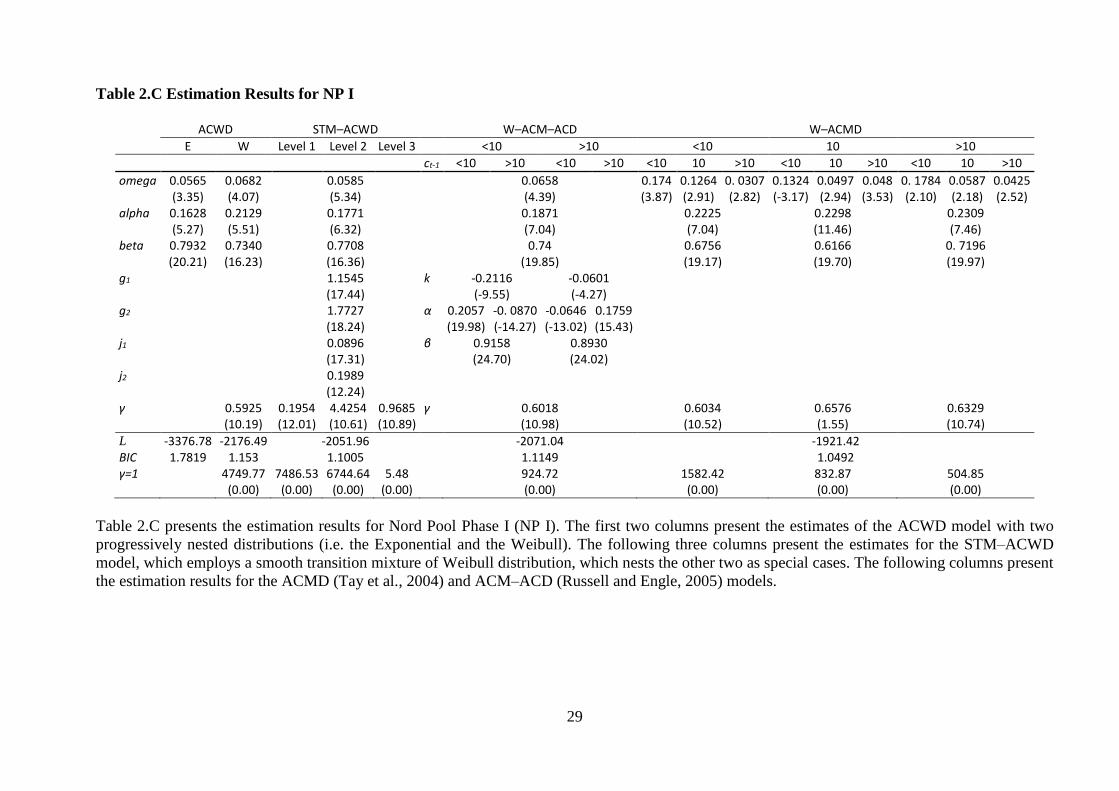
29

Table 2.C Estimation Results for NP I



ct-1 <10 >10 <10 >10 <10 10 >10 <10 10 >10 <10 10 >10

omega 0.0565 0.0682 0.0585 0.0658 0.174 0.1264 0. 0307 0.1324 0.0497 0.048 0. 1784 0.0587 0.0425 (3.35) (4.07) (5.34) (4.39) (3.87) (2.91) (2.82) (-3.17) (2.94) (3.53) (2.10) (2.18) (2.52) alpha 0.1628 0.2129 0.1771 0.1871 0.2225 0.2298 0.2309 (5.27) (5.51) (6.32) (7.04) (7.04) (11.46) (7.46) beta 0.7932 0.7340 0.7708 0.74 0.6756 0.6166 0. 7196 (20.21) (16.23) (16.36) (19.85) (19.17) (19.70) (19.97) g1 1.1545 k -0.2116 -0.0601 (17.44) (-9.55) (-4.27) g2 1.7727 α 0.2057 -0. 0870 -0.0646 0.1759 (18.24) (19.98) (-14.27) (-13.02) (15.43) j1 0.0896 β 0.9158 0.8930 (17.31) (24.70) (24.02) j2 0.1989 (12.24) γ 0.5925 0.1954 4.4254 0.9685 γ 0.6018 0.6034 0.6576 0.6329 (10.19) (12.01) (10.61) (10.89) (10.98) (10.52) (1.55) (10.74)

L -3376.78 -2176.49 -2051.96 -2071.04 -1921.42 BIC 1.7819 1.153 1.1005 1.1149 1.0492 γ=1 4749.77 7486.53 6744.64 5.48 924.72 1582.42 832.87 504.85 (0.00) (0.00) (0.00) (0.00) (0.00) (0.00) (0.00) (0.00)

Table 2.C presents the estimation results for Nord Pool Phase I (NP I). The first two columns present the estimates of the ACWD model with two




30

Table 2.D Estimation Results for NP II



ct-1 <10 >10 <10 >10 <10 10 >10 <10 10 >10 <10 10 >10

omega 0.1101 0.1542 0.1161 0.1120 0.5413 0.3974 0.1491 0.3644 0. 3285 0.0583 0.3981 0.2119 0.0020 (1.92) (1.96) (2.61) (7.33) (5.30) (5.18) (3.35) (4.65) (3.56) (1.96) (5.07) (2.68) (1.13) alpha 0.0968 0.1363 0.1085 0.1625 0.2003 0.2522 0.198 (3.15) (2.95) (4.00) (7.89) (7.06) (5.86) (4.04) beta 0.8065 0.7277 0.7859 0.7139 0.5396 0.5651 0.5847 (10.21) (6.58) (11.86) (9.74) (8.74) (9.83) (10.03) g1 1.6524 k -0.3447 -0.2392 (13.82) (-11.25) (-15.79) g2 1.1974 α 1.1953 -0. 5044 -0.6099 2.2741 (14.17) (7.63) (-8.91) (-14.25) (18.81) j1 0.0544 β 0.8956 0.7864 (15.53) (17.24) (16.89) j2 0.2469 (15.96) γ 0.5979 0.2216 6.1974 0.8652 γ 0.6338 0.6242 0.6493 0.6615 (9.50) (18.17) (18.97) (20.61) (22.20) (16.86) (14.68) (13.67)

L -3818.78 -2761.02 -2633.17 -2557.75 -2515.10 BIC 2.1248 1.5404 1.4832 1.4459 1.4358 γ=1 4387.13 164.75 32291.7 7.84 3215.72 1171.47 691.48 353.41 (0.00) (0.00) (0.00) (0.00) (0.00) (0.00) (0.00) (0.00)

Table 2.D presents the estimation results for Nord Pool Phase II (NP II). The first two columns present the estimates of the ACWD model with two




31

Table 3.Trading Intensity, Q–stat (15) and In-Sample Performance

Q–stat (15) Rank ECX I P-value Rank ECX II P-value Rank NP I P-value Rank NP II P-value

ACWD E 3 8.23 (0.91) 3 6.26 (0.98) 2 1.24 (1.00) 3 3.17 (1.00) W 2 1.22 (1.00) 2 5.37 (0.99) 3 1.25 (1.00) 2 3.16 (1.00)

STM–ACWD 1 0.40 (1.00) 1 4.59 (1.00) 1 1.15 (1.00) 1 3.13 (1.00)

W-ACM–ACD 5 71.40 (0.00) 5 69.78 (0.00) 5 77.88 (0.00) 5 28.94 (0.88) W-ACMD 4 67.12 (0.00) 4 58.25 (0.00) 4 65.06 (0.00) 4 27.61 (0.94)

UNL CORR

Rank ECX I Rank ECX II Rank NP I Rank NP II Rank ECX I Rank ECX II Rank NP I Rank NP II

In-s

amp

le

fore

cast

s ACWD E 3 7.4972 3 5.2873 3 2.9530 3 1.5438 3 0.3253 3 0.2179 3 0.3116 3 0.2080

W 2 7.2839 2 5.2379 2 2.8882 2 1.5210 2 0.3502 2 0.2218 2 0.3118 2 0.2090

STM–ACWD 1 6.9638 1 5.1546 1 2.3593 1 1.4370 1 0.3626 1 0.2310 1 0.3307 1 0.2100

W-ACM–ACD 4 8.4493 4 6.9867 4 3.2812 4 1.5734 4 0.2671 4 0.2017 4 0.2944 4 0.1880

W-ACMD 5 8.5104 5 7.6794 5 3.4230 5 1.6990 5 0.2567 5 0.1982 5 0.2866 5 0.1783

1-s

tep

fore

cast

s ACWD E 3 7.2627 3 6.7554 3 8.2769 3 3.7380 3 0.0882 3 0.1728 3 0.1939 3 0.1033

W 2 6.3353 2 5.5994 2 8.1989 2 3.5152 2 0.0921 2 0.1799 2 0.1971 2 0.1239

STM–ACWD 1 6.1559 1 4.8021 1 7.9173 1 3.0387 1 0.0953 1 0.1826 1 0.2179 1 0.1421

W-ACM–ACD 4 7.4320 4 6.9406 4 9.8608 4 3.9946 4 0.0818 4 0.1590 4 0.1920 4 0.0977

W-ACMD 5 8.0481 5 7.7937 5 10.7348 5 4.3293 5 0.0791 5 0.1477 5 0.1821 5 0.0905

10

-ste

p

fore

cast

s ACWD E 1 2.7956 1 5.4895 1 3.6964 1 2.8947 1 0.0111 1 0.2578 1 0.0384 1 0.0539

W 2 2.9078 2 6.4553 2 3.7362 2 2.9387 2 0.0100 2 0.2144 2 0.0366 2 0.0420

STM–ACWD 3 2.9145 3 7.6463 3 3.7800 3 2.9486 3 0.0062 3 0.2031 3 0.0356 3 0.0325

W-ACM–ACD 5 11.8853 5 25.7027 5 20.5339 5 20.1126 5 0.0013 5 -0.0025 4 0.0096 5 -0.0087

W-ACMD 4 8.1354 4 22.7088 4 20.4245 4 19.8071 4 0.0017 4 0.0013 5 0.0084 4 -0.0080

Table 3 presents the ranking of all models employed, namely the ACWD with the Exponential, the Weibull or a smooth transition mixture of Weibull

distributions, as well as the ACMD and ACM–ACD with the Weibull distribution. The top panel reports the ranking according to Q–statistic, while the

lower panel reports the ranking according to in–sample 1–step, as well as out–of–sample 1–step and 10–step forecasts, employing the unitised loss and

correlation performance measures (explained in the appendix).

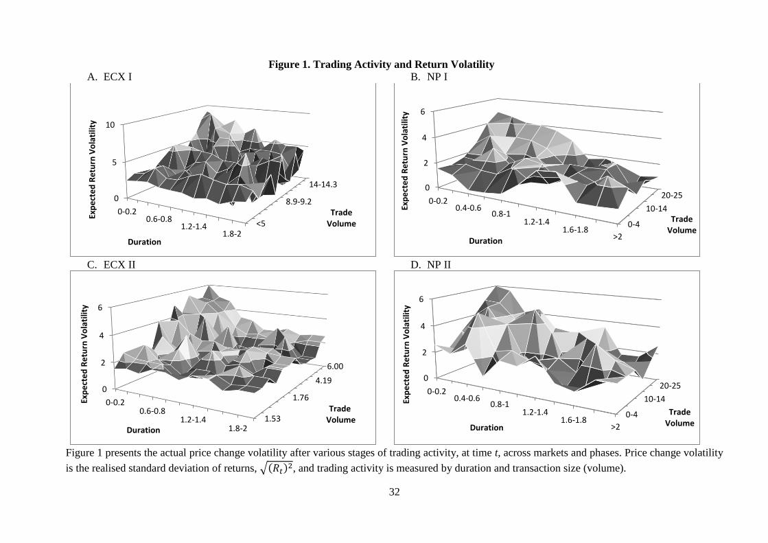
32

Figure 1. Trading Activity and Return Volatility

A. ECX I B. NP I

C. ECX II D. NP II

Figure 1 presents the actual price change volatility after various stages of trading activity, at time t, across markets and phases. Price change volatility

is the realised standard deviation of returns, √(𝑅𝑡)2, and trading activity is measured by duration and transaction size (volume).

0-0.20.6-0.8

1.2-1.41.8-2

0

5

10

<5

8.9-9.2

14-14.3

Duration

Exp

ect

ed

Re

turn

Vo

lati

lity

Trade Volume 0-4

10-14

20-250

2

4

6

0-0.20.4-0.6

0.8-11.2-1.4

1.6-1.8>2

Trade Volume

Exp

ect

ed

Re

turn

Vo

lati

lity

Duration

0-0.20.6-0.8

1.2-1.41.8-2

0

2

4

6

1.53

1.76

4.19

6.00

Duration

Exp

ect

ed

Re

turn

Vo

lati

lity

TradeVolume

0-4

10-14

20-250

2

4

6

0-0.20.4-0.6

0.8-11.2-1.4

1.6-1.8>2

Trade Volume

Exp

ect

ed

Re

turn

Vo

lati

lity

Duration

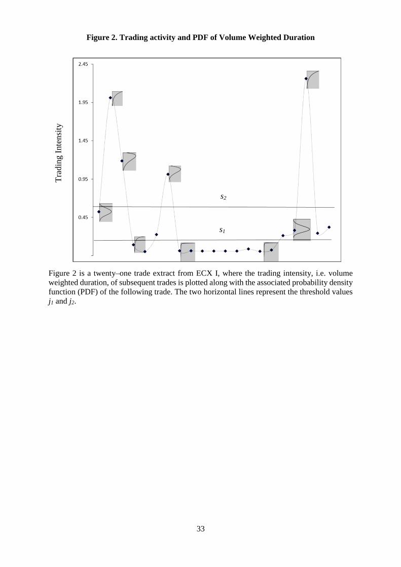
33

Figure 2. Trading activity and PDF of Volume Weighted Duration

Figure 2 is a twenty–one trade extract from ECX I, where the trading intensity, i.e. volume

weighted duration, of subsequent trades is plotted along with the associated probability density

function (PDF) of the following trade. The two horizontal lines represent the threshold values

j1 and j2.

Tra

din

g I

nte

nsi

ty

s1

s2

34

Figure 3. Price Change Volatility around High Trading Intensity Trades During the Day

A. ECX I B. NP I

C. ECX II D. NP II

Figure 3 presents the actual price change volatility, √(𝑅𝑡)2, five transactions before and twenty transactions after a high trading intensity trade, across

markets and phases.

08

10

13

150

1

2

3

4

Time of Day

Pri

ce C

han

ge V

ola

tilit

y

Event Time

08

10

12

140

2

4

6

Time of Day

Pri

ce C

han

ge V

ola

tilit

y

Event Time

8

10

13

150

1

2

3

t-5

t-2

t+1

t+4

t+7

t+1

0

t+1

3

t+1

6

t+1

9

Time of Day

Pri

ce C

han

ge V

ola

tilit

y

Event Time

08

10

12

140

1

2

3

t-5

t-2

t+1

t+4

t+7

t+1

0

t+1

3

t+1

6

t+1

9

Time of Day

Pri

ce C

han

ge V

ola

tilit

y

Event Time

35

Figure 4. Number of Trades

A. ECX

B. NP

Figure 4 presents the total number of trades during the day, across markets and phases, along

with the total number of high trading intensity and OTC trades.

0

2

4

6

8

10

12

14

16

0

5

10

15

20

25

30

35

40

45

50

8 9 1011121314151617 8 9 1011121314151617 8 9 1011121314151617

2006 2007 2008

# o

f To

tal T

rad

es (

x 1

00

0)

# o

f O

TC &

Hig

h T

.I. T

rad

es (

x 1

00

)

# of Total Trades # of High ti

0

100

200

300

400

500

600

700

800

900

0

20

40

60

80

100

120

140

160

08 09 10 11 12 13 14 15 08 09 10 11 12 13 14 15 08 09 10 11 12 13 14 15

2006 2007 2008

# o

f To

tal T

rad

es

# o

f O

TC a

nd

Hig

h T

.I. T

rad

es

# of Total Trades # of High T.I.

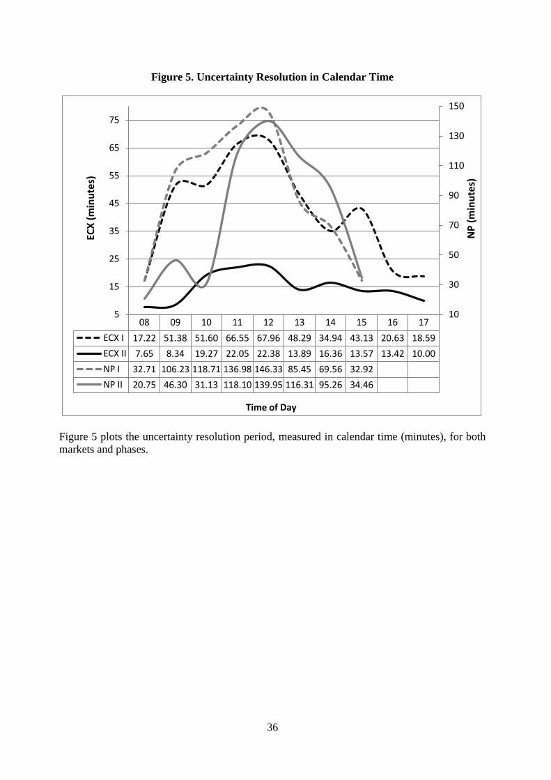
36

Figure 5. Uncertainty Resolution in Calendar Time

Figure 5 plots the uncertainty resolution period, measured in calendar time (minutes), for both

markets and phases.

08 09 10 11 12 13 14 15 16 17

ECX I 17.22 51.38 51.60 66.55 67.96 48.29 34.94 43.13 20.63 18.59

ECX II 7.65 8.34 19.27 22.05 22.38 13.89 16.36 13.57 13.42 10.00

NP I 32.71 106.23 118.71 136.98 146.33 85.45 69.56 32.92

NP II 20.75 46.30 31.13 118.10 139.95 116.31 95.26 34.46

10

30

50

70

90

110

130

150

5

15

25

35

45

55

65

75

NP

(m

inu

tes)

ECX

(m

inu

tes)

Time of Day

Liquidity and resolution of uncertainty in the European ...

Documents

Transcript of Liquidity and resolution of uncertainty in the European ...