Liquid Assets in Banks: Theory and Practice

Guillermo Alger and Ingela Alger�

November 1999

Abstract

This paper summarizes theoretical �ndings on the determinants of liquid assets held by

banks. The �ndings are summarized in a series of predictions, some of which are tested

using a panel data set on Mexican banks. Surprisingly, we �nd that banks with relatively

more demand deposits have relatively less liquid assets, in contrast with the theoretical

prediction. We further exploit a period characterized by a prolonged aggregate liquidity

shock on the Mexican banking system to shed light on the question: are there banks

that rely more than others on liquid assets to meet their liquidity needs? We �nd that

only small banks seem to rely on liquid assets to meet severe liquidity shocks.

JEL Classi�cation: G21; G28

Keywords: Liquid Assets; Banks; Liquidity Shocks

�Analysis Group Economics (galger@analysisgroup.com) and Boston College (ingela.alger@bc.edu), re-

spectively. We thank Jean Tirole, Esther Du o, Xavier Freixas, Denis Gromb, Sendhil Mullainathan and

Dimitri Vayanos for very useful comments and discussions. We are also grateful to Patricio Bustamante

and the Comisi�on Nacional Bancaria y de Valores (M�exico) for the data set, and to several bankers and

regulators from the U.K., U.S. and Mexico for interesting discussions. This research was initiated while the

authors were visiting the Financial Markets Group at the London School of Economics, and we would like to

thank them for their hospitality, as well as for comments from FMG lunch seminar participants. We alone

are responsible for any remaining errors.

1 Introduction

The subject of this paper is liquid assets held by banks. Our objective is to provide a

comprehensive picture of this issue, by reviewing existing theory and empirical �ndings,

and by providing some tests of theoretical predictions, using new data.

Broadly, the two main activities of banks are to accept funds through deposits and to

grant loans. A bank may however choose not to invest all its available funds in (typically

long-term) loans; indeed, it may keep some of the funds in cash (or reserves at the central

bank) and/or invest in marketable securities such as Treasury bills and bonds. The main

feature distinguishing these assets from regular bank loans is that they are more liquid. But

liquidity usually comes at a price, since liquid assets yield lower returns. A glance at banks'

balance sheets1 reveals that a substantial part of available funds are indeed invested in

liquid assets: adding up securities, dues from depository institutions, and cash, the average

holding of liquid assets in U.S. commercial banks in 1998 was 24.4% of total assets. Since

the returns are typically low, the question is: why do banks hold liquid assets?

Our analysis of this question begins with a review of existing theories, including those which

do not focus directly on how banks determine their level of liquid assets, but which do carry

implications for that. We distinguish four broad categories of theories. In the �rst one,

the portfolio management theory developed in the 50's and 60's, risk aversion plays an

important role in explaining the level of liquid assets chosen by a bank. In contrast, all

other theories assume that banks are risk neutral. The second group of theories analyzes

the determinants of credit supply and deposit demand, viewing liquid assets as the residual

between, on the one hand, the bank's equity and liabilities, and on the other hand, the credit

portfolio. These two �rst categories of theories do not explicitly take into account one of

the speci�cities of banks, namely, that they face potentially large, random liquidity shocks

(due to unpredictable deposit withdrawals, and or unpaid credits). Presumably, banks that

aim at staying in business wish to keep a good reputation concerning its ability to meet

liquidity demands. As a result, banks may want to keep liquid assets in order to be able to

1See the appendix for a brief introduction to the items on a bank's balance sheet. For a detailed expla-

nation, the reader may consult Garber and Weisbrod (1992) or Hempel, Simonson and Coleman (1994), for

instance.

meet large liquidity shocks, as suggested by the \liquid assets as a bu�er" theories. These

theories are however silent on one important question: to what extent may banks rely on

increased liabilities to raise liquidity on short notice (e.g., by selling CDs or borrowing from

other banks)? Indeed, these theories assume an exogenously given penalty rate if the bank is

not able to meet a liquidity need, without modeling the liability side of the bank's liquidity

management. This is an important shortcoming, since increased liabilities at �rst sight

do appear as a cheap substitute for liquid assets: indeed, by relying on liabilities, banks

do not need to tie up important sums of money during long periods of time in order to

withstand occasional future shocks. Recent theories have started investigating the trade-o�

between assets and liabilities to meet liquidity needs. These theories focus on information

asymmetries to explain a bank's limited borrowing capacity.

We summarize the theoretical results in a series of empirical predictions. We also make the

observation that most predictions relate to a bank's choice of liquid assets before a liquidity

shock occurs. In reality, banks face liquidity shocks every day, together with the decision

of how to invest in liquid assets for future needs, the net e�ect still being an unresolved

theoretical question. In our empirical analysis, introduced next, we exploit the fact that

our data covers a period with a dramatic liquidity shock to shed some light on the question:

can we distinguish banks that rely more on liquid assets to meet their liquidity needs than

others?

The empirical analysis �rst provides tests of some of the theoretical predictions. We use a

panel data set for the Mexican banking system, from January 1997 to March 1999. Based on

the observation of several facts (tightening of monetary policy, political uncertainty related

to the banking system, and a strain on the Mexican economy due to a sharp decrease in the

oil prices and the worldwide �nancial crisis in 1998), and comforted by econometric tests,

we are able to distinguish two periods: one characterized by \normal" conditions (January

1997-Fabruary 1998), and the second one characterized by an aggregate, prolonged liquidity

shock on the Mexican banking system (March 1998-March 1999). As a result, we use the

�rst period to test the predictions concerning bu�er-building, and the second one to shed

some light on the above mentioned question, i.e., which banks rely more heavily on liquid

assets to meet their liquidity needs.

2

2 Review of Theoretical Findings

Before starting the review, it is necessary to provide a more precise de�nition of liquid as-

sets. An asset is liquid if it can be sold quickly without signi�cant losses. What determines

the liquidity of an asset is still a disputed issue among theorists, and we will not review

that literature here.2 Instead, we will adopt the conventional wisdom found in the bank

management literature,3 an asset is liquid if it is widely known to have low risk (such as

government debt) and if it has a short maturity (a short maturity implies that the asset's

price is less sensitive to interest rate movements, making large capital losses unlikely). The

typical bank assets which are liquid according to that de�nition include cash, reserves rep-

resenting an excedent as compared to reserves required by law4, securities (e.g., government

debt, commercial paper), and interbank loans with very short maturity (one to three days).

2.1 The portfolio management theory

According to Pyle (1971) and Hart and Ja�ee (1974), a bank's assets and liabilities may

all be viewed as securities. As a result of this interpretation, the whole bank may actually

be considered as a portfolio of securities. Once that view is postulated, it is possible to

apply the portfolio theory developed in the 50's and 60's to the asset-liability management

of a bank. The following simple model, adapted from Freixas and Rochet (1997, p.236)

illustrates the main ideas.

Assume for simplicity that there is only one risky �nancial security (which may be in-

terpreted as loans), and one risk-free security (the liquid asset), with returns ~rL and r,

respectively. Starting with initial wealth E + D (equity and deposits, taken as an exoge-

nously given amount here), the bank manager determines the amounts xL to invest in the

risky security, the rest being invested in the risk-free, liquid asset.5 A positive amount is

2See the literature initiated by Kyle (1985), and also O'Hara (1995) for a review.

3See Garber and Weisbrod (1992) and Hempel et al. (1994) for instance.

4Indeed, reserves (i.e., funds held in the account at the central bank) are totally illiquid if they serve to

comply with a reserve requirement.

5In this model, the bank manager is assumed to act fully in line with the bank owners objectives, i.e.,

there are no agency problems here.

3

interpreted as being on the asset side of the balance sheet, and a negative amount on the

liability side. Assuming for simplicity that the interest rate on deposits is zero, the random

payo� is equal to:6

~� = r(E +D) + (~rL � r)xL:

The bank manager is risk averse, and assumed to have mean-variance preferences: U(E(~�); var(~�)),

with U increasing in the expected pro�t, and decreasing in the variance. Given these

premises, the following result obtains: if the expected returns are ordered in the following

way, �rL > r > 0 then xL > 0.

When it comes to the amount invested in liquid assets, E + D � xL, the most important

determinant is risk, i.e., both the level of risk aversion, and the riskiness of the returns on

loans. First, E + D � xL is increasing in the degree of risk aversion of the manager (for

low degrees of risk aversion, it may be negative). Hence, banks with relatively more liquid

assets should be more risk averse. Furthermore, for a given function U , and for given excess

returns (�rL � r), the amount invested in liquid assets is increasing in var(~rL), keeping �rL

constant. An empirical implication is that, when the volatility of interest rates increases,

banks should decrease the amount of loans, and increase the holdings of liquid assets.

Another important implication of this theory is that, if deposits and equity are also in-

terpreted as securities (i.e., if E and D are endogenized), then the size of the bank is

indeterminate. This follows simply from the fact that in that case, any multiple of the

portfolio which is optimal for a given level of equity and deposits, is also optimal. As a

result, size should be a random variable, and the proportion of liquid assets to total assets

should be independent of size.

2.2 Liquid assets as a residual: the role of supply and demand

The portfolio management theory of banking described above assumes that the bank man-

ager is risk averse. Such an assumption could be defended for small, manager-owned banks.

6In a more realistic model, the deposit interest rate would have to be determined endogenously. Here

that is disregarded, the focus being on the e�ect of risk aversion on the bank's balance sheet.

4

However, for banks owned by shareholders who have well-diversi�ed stock portfolios, risk

neutrality seems to be a more appropriate assumption. Henceforth, risk neutrality is as-

sumed. Given that the returns on liquid assets are typically lower than those on regular

bank loans, the question immediately arises of why any bank would invest in liquid securities

at all.

One way of dealing with the question is to view liquid assets as the di�erence between equity

plus deposits and credits, and apply a classical microeconomic analysis of the determinants

of deposits and credits in terms of supply and demand (taking equity as given). This

contrasts with the portfolio management theory in which the supply of deposits and demand

of credits are perfectly elastic.

According to this theory, banks sell credit, using deposits as inputs. Accepting deposits

imply certain administrative costs, as does giving credits. These costs may be summarized in

two separate cost functions. If the demand for credit and supply of deposits are exogenously

given functions, then the standard marginal cost equals marginal revenue rule may be

applied to determine the amounts of credits supplied and deposits demanded by the bank.

From basic microeconomic analysis, we know that these will depend on the shape of the

cost functions and market structure. Thus for a given market structure, di�erences in

balance sheet compositions could be traced to di�erences in cost functions. As a bank's

cost functions are not observable by outsiders, it is however diÆcult to state meaningful

empirical implications using this approach.

A conceptually di�erent determinant of credit supply is introduced when considering bor-

rowers' default risk. Indeed, as shown by Stiglitz and Weiss (1981) and Bester and Hellwig

(1987),7 adverse selection or moral hazard may lead to credit rationing, in the sense that

there does not exist an interest rate for which the (competitive) market clears. For instance,

in the adverse selection case, an increase in the credit interest rate leads to a riskier popu-

lation of borrowers, which in turn potentially implies a non-monotonic credit supply. If the

supply and demand curves do not intersect, credit is rationed. Compared to the competitive

outcome mentioned above, credit supply is smaller, and ceteris paribus, the investment in

7Although the models in these papers do not include banks' decisions to invest in liquid assets, we believe

the ideas exposed in them can be used to (partially) explain why a bank, for a given amount of deposits,

would limit its credits, thereby investing part of the funds available through deposits in liquid assets.

5

liquid assets should then be larger. An implication of that theory is that, given a level of

deposits, the liquid assets held by banks should increase if the population of borrowers is

believed to have become more risky, as could be expected during an economic recession for

instance.

2.3 Liquid assets as a bu�er

All the above mentioned models make an important simpli�cation: they do not take into

account the unpredictability of deposit withdrawals, or other factors a�ecting the uncer-

tainty of ows in and out of the bank, and the e�ects thereof. In contrast, a number of

researchers have sought to model the e�ects of the liquidity risk implied by these uncertain-

ties. We review the insights concerning liquid assets, starting with models in which banks

invest in liquid assets for purely precautionary motives. That line of research was initiated

by Edgeworth (1888), and was further developed during the 1960's (see, e.g., Porter (1961),

and Kane and Malkiel (1965)).

A simple model, taken from Freixas and Rochet (1997, p.228), is useful to develop the

main insights. The two-period model features a bank deciding the amount x to invest in

liquid assets out of the funds available through an exogenously given amount of deposits

and equity, xD + E, the rest being invested in illiquid loans. Interest rates are given and

ordered as previously: rL > r > rD. A period after the investment decision, some deposits

are withdrawn and new deposits arrive; the net result is the realization w of the random

variable ~w (this is the only uncertainty in the model). If w exceeds the reserves x, the

bank su�ers a liquidity shortage; it must then pay a penalty rP (w � x) (we will comment

further on the interpretation of rP below), where rP > rL. Assuming again for simplicity

that rD = 0, the objective of the bank is to maximize the expected pro�t:

�(x) = rL(xD + E � x) + rx� rPE[max(0; ~w� x)]:

The �rst-order condition is:

�0(x) = �(rL � r) + rPProb[ ~w � x]:

6

This expression determines the optimal amount of liquid assets x� as follows:8

Prob[ ~w � x�] =

rL � r

rP

:

The empirical implications are clear and intuitively appealing. First, the amount invested

in liquid assets decreases with the opportunity cost of investing in liquid assets, rL � r.

Second, it increases when high values of ~w become more likely in the sense of �rst-order

stochastic dominance. Note however that if the distribution of ~w becomes more risky in the

sense of second-order stochastic dominance, the e�ect on x� is not clear; it could go either

way, depending on the exact shift in the distribution. Finally, it is increasing in the penalty

rate rP .

Several di�erent interpretations of the penalty rate are possible. In a system where banks

can easily turn to the central bank for advances, it can be interpreted as the discount rate

(i.e., the rate charged by the central bank), which in such a system is typically higher than

other rates. In a system where such credits are not automatically given, it could be the rate

at which the bank may obtain funding on the �nancial markets or the interbank market, or

the cost of liquidating illiquid assets.

In their model on why banks traditionally tie together the activities of deposit-taking and

lending, Kashyap, Rajan and Stein (1998) analyze a situation very similar to the one de-

scribed above. The main di�erence is that the expected deposit withdrawal is proportional

to the total amount of deposits. One prediction obtained in that paper is that banks with

relatively more demand deposits should hold relatively more liquid assets (an increase in

demand deposits corresponding to a shift in the shock distribution in the sense of �rst order

stochastic dominance).

8Again risk aversion is not necessary for positive amounts of liquid assets to obtain. Nevertheless, the

amount of liquid assets would be a�ected by the introduction of deposit insurance. Indeed, deposit insurance

should lead banks to maximize risk, as shown by Merton (1977). Banks may however be interested in

investing in liquid assets despite deposit insurance, for instance in order to protect their charter value, as

suggested by Marcus (1984).

7

2.4 Liquid assets and liabilities: the role of market imperfections

The above mentioned approach does not explicitly model the liability side of a bank's bal-

ance sheet as a liquidity source. It is only implicitly present through the penalty rate. This

rate being exogenous and independent of the needed amount ~w� x�, the cost of increasing

liabilities (e.g., by issuing CDs, by borrowing from other banks or from the central bank)

is assumed exogenous, and the bank's access to these liabilities is not restricted. Recog-

nizing the importance of liabilities as a liquidity source, Poole (1968) includes interbank

borrowings in a classical inventory model applied to banking. The model suggested by

Poole is however not entirely satisfactory, since it takes the supply of funds on the inter-

bank market as perfectly elastic. The approach found in the recent literature seems more

promising in yielding new insights into the liquid assets question; in sharp contrast with

preceding theories, this approach seeks to explain why banks may only have limited access

to liabilities.

The market imperfections that have been studied are due to informational asymmetries.

Holmstr�om and Tirole (1998) analyze the e�ects of moral hazard, whereas Lucas and Mc-

Donald (1992) focus on adverse selection.

In the model suggested by Holmstr�om and Tirole (1998), �rms (and therefore banks) en-

counter problems when raising external �nance due to moral hazard (i.e., the manager

misallocates resources unless given proper incentives). Moral hazard implies that the bank

cannot pledge the full value of an investment project to outside investors. The bank makes

a long-term investment which may need extra funding at an interim stage due to a liquidity

shock. The crucial insight is that due to the moral hazard an ineÆcient decision may be

taken at that stage: indeed, there exist liquidity shocks which are small enough to make

further investment economically viable, but which are at the same time large enough to

make outside investors unwilling to invest (since they cannot recover the full value). A way

to avoid this ineÆciency is to invest in liquid assets beforehand, as this removes any need

to seek external �nance at the critical interim stage. The authors determine the amount

of liquid assets chosen by the bank. Due to the linearity of the model, the only relevant

factor for the determination of the amount of liquid assets is the distribution of the liquidity

shock. When the distribution of the liquidity shock is riskier in the sense that larger shocks

become more likely overall (i.e., in the sense of �rst-order stochastic dominance) the optimal

8

amount of liquid assets is larger.9 However, when the distribution of the liquidity shock

is riskier in the sense of a mean preserving spread (second-order stochastic dominance),

the optimal amount of liquid assets decreases. This results from the fact that when the

distribution is riskier in that sense, on the margin the investment in liquid assets implies

a lower increment of insurance: the achieved increase in the probability of continuation is

smaller than with the less risky distribution. Therefore, the bank \buys" less insurance,

and instead invests more in the illiquid project.10 11

Lucas and McDonald (1992) build on the insight of Myers and Majluf (1984) that private

information about asset quality a�ects a bank's (or more generally, a �rm's) ability to

raise external �nance.12 They consider a bank which may need external �nance due to

a deposit shortcoming. As opposed to deposits, external �nance is uninsured, and thus

sensitive to information about the bank's asset quality, which may be high or low. The

asset quality being private information, good and bad banks would pay the same rate for

external funding if they could not signal their quality (i.e., in a pooling equilibrium). Good

banks therefore have an incentive to signal themselves as good, and the signaling device

they use is the level of liquid assets. The intuition is as follows: while the bene�t of being

perceived as a good bank instead of a bad one is the same for both types of banks (through

the lower funding cost), the cost of investing in liquid assets is higher for the bad banks.

This follows from the fact that bad banks survive only if they receive a high return on

future loans: conditional upon surviving, bad banks therefore have a high average return

per unit invested. As a result, the opportunity cost of investing in liquid (low-yield) assets

is high. By contrast, a good bank survives even if the return on future loans is low. Hence,

conditional upon surviving, good banks have a lower average return per unit invested than

9Note that this result again obtains in a model with only risk-neutral agents.

10The above predictions are valid for banks' investments in securities, only insofar as stored liquidity is

preferred to credit lines. Indeed, as the authors point out, in their framework a perfect substitute for storing

liquid assets through securities is the negotiation of an irrevocable credit line up to the desired amount.

11Rochet and Tirole (1996) propose an extension of this model, applied to interbank lending. They

analyze how peer monitoring a�ects the liquidity needs of lending and borrowing banks. Since the liquidity

shock structure is similar to the one in Holmstr�om and Tirole (1998), the model yields similar predictions

concerning liquid assets.

12The paper endogenizes the level of liquid assets (�nancial slack), which was exogenous in Myers and

Majluf (1984).

9

bad banks, implying a lower opportunity cost. Therefore, good banks may signal themselves

by investing in liquid assets, and they �nd that pro�table under certain conditions. The

model proposed by Lucas and McDonald thus leads to the prediction that, given a level of

deposits and a withdrawal distribution function, good banks should invest more in liquid

assets than bad banks.

2.5 Liquid assets and the interbank market

Last, we consider two papers that are concerned with interbank markets. Bhattacharya and

Gale (1987) and Alger (1999) analyze the role of interbank markets for the allocation of liq-

uidity. In both papers, and in a similar vein to some of the above mentioned models, banks

choose the amounts to invest in liquid assets and in high-yield but illiquid loans, given that

there is uncertainty concerning the amount of deposit withdrawals before the loans mature.

Assuming away any aggregate uncertainty concerning the early deposit withdrawals, eÆ-

ciency (in the sense that there is not aggregate under-investment in loans) may be attained

through the existence of an interbank market: all banks choose the level of liquid assets

corresponding to the expected deposit withdrawal, and when the withdrawals realize, banks

with a liquidity shortage borrow from banks with a liquidity surplus. Bhattacharya and

Gale (1987) and Alger (1999) analyze two di�erent potential sources of imperfection of the

interbank market, with di�erent empirical implications.

Bhattacharya and Gale (1987) focus on the implications of asymmetric information about

the amount invested in liquid assets. If this amount is not observable to outsiders, a free

rider problem arises, implying that there is an aggregate shortage of liquidity when the

early deposit withdrawals occur. The authors suggest that reserve requirements could be

an answer to such a market failure.

Alger (1999) assumes that the amount of liquid assets is observable, and instead analyzes

an interbank market characterized by credit risk. At the time the banks seek additional

liquidity, they have private information about their solvency. The credit risk may lead the

interbank market collapse; hence in this framework, the interbank market is not always able

to provide liquidity insurance to banks, as it would without the adverse selection problem.

This a�ects the banks' investment in liquid assets, which is determined before banks know

10

whether they are solvent or not. If banks foresee that the interbank market will collapse,

they store a suÆcient amount of liquid assets to withstand large deposit withdrawals.13

In that case, there is over-investment in liquid assets compared to the situation in which

the interbank market functions properly. Furthermore, banks with relatively more equity,

having a higher stake at risk, invest relatively more in liquid assets.

The model also carries implications in terms of economic cycles. Indeed, the model incor-

porates the notion of correlation between the banks' returns. Thus, a high (resp. low)

probability that the bank is solvent combined with a high correlation between the banks'

returns, may be interpreted as an economic boom (resp. recession). The results of the

model thus indicate that the risk of an interbank market collapse is greater during eco-

nomic recessions, or if the correlation between the banks' returns is highly negative. Thus,

if a recession is expected, banks should invest more in liquid assets.

2.6 Summary of predictions

Before turning to the empirical evidence, we summarize the predictions obtained through

the above described theories.

Prediction 1 The relative amount of liquid assets increases when their opportunity cost

(i.e., the di�erence in returns on loans and on securities) decreases.

Most of the above theories yield this prediction, which may at �rst seem trivial.14 Interest-

ingly, however, the prediction challenges the conventional wisdom that high levels of liquid

assets imply low returns. Indeed, due to technological15 and strategic16 di�erences, the

13In a sense, this is related to the models focusing on liquid assets as a bu�er; in the case of interbank

market collapse, the penalty rate rP of those models is in�nitely high.

14Note that in a general equilibrium framework, the level of liquid assets chosen would in turn a�ect the

opportunity cost.

15Examples include di�erences in management quality, in credit analysis models used by the bank, and in

securities analysis.

16For instance specialization of the loan portfolio in di�erent sectors, or of the securities portfolio in

di�erent instruments.

11

returns on both the loans and the securities portfolios may di�er across banks. Therefore a

high level of securities does not necessarily imply a lower level of returns.17

Prediction 2 The relative amount of liquid assets is higher if larger liquidity shocks are

more likely in the sense of �rst order stochastic dominance.

This intuitively appealing prediction obtains in the bu�er theory and in Holmstr�om and

Tirole (1998). Now, when do larger liquidity shocks become overall more likely? An oc-

currence which immediately comes to mind is seasonal uctuations. For instance, all banks

face larger withdrawals before holidays. Also, banks lending to sectors a�ected by seasonal

patterns in their production (such as the agricultural sector) do experience larger with-

drawals during certain months of the year. Furthermore, the level of deposits may a�ect

the expected liquidity shock. One may assume that banks that withdrawals are propor-

tional to the level of deposits, as in Kashyap et al. (1998). In other words, more deposits

simply means that the distribution of withdrawals shifts to the right. Hence, given that

assumption:

Prediction 3 Banks with relatively more demand deposits have relatively more liquid as-

sets.

The following prediction obtains in Holmstr�om and Tirole (1998) and in Rochet and Tirole

(1996).

17The following simple portfolio model (adapted from section 2.1) illustrates this. The bank has to

determine the amount xL to invest in loans, given a liability size E + D, the rest being invested in the

risk-free liquid asset. Suppose that the manager has the following speci�c mean-variance utility function:

U(E(~�);var(~�)) = E(~�)� 1

2var(~�). Letting var(~�) � �

2 be the constant variance of the return ~rL, we get:

U(E(~�);var(~�)) = r(E +D) + (~rL � r)xL �1

2�2x2

L, giving the �rst-order condition: xL =(~rL � r)

�2. Hence,

the amount invested in the liquid asset (E + D � xL) is decreasing in its opportunity cost (~rL � r). Now,

one bank (say bank A) may, for the reasons mentioned in the text, have higher returns than bank B both

on its security portfolio, and on its loans. Using a superscript to denote the individual bank: rA > rB and

rA

L > rB

L . Given this, it may well be that rAL � rA < rB

L � rB , i.e., that the opportunity cost of investing in

securities is smaller in the more pro�table bank. Hence, banks with relatively more liquid assets need not

be the least pro�table.

12

Prediction 4 If large and small shocks become more likely, and average-sized shocks become

less likely (i.e., if a distribution of shocks is riskier in the sense of second-order stochastic

dominance), the amount of liquid assets decreases.

The intuition behind this is clear as well: when the distribution of shocks is a�ected in the

sense of second-order stochastic dominance, the marginal bene�t of investing in liquid assets

may become smaller (the probability that the liquid asset will enable the bank to survive a

liquidity shock becomes smaller when large shocks become more likely). An example of the

distribution of liquidity shocks becoming more risky in the sense of second-order stochastic

dominance, is an overall increase in the volatility of interest rates and foreign exchange

rates, for instance.

Prediction 5 The relative amount of liquid assets increases with the volatility of the returns

on risky assets (loans).

This obtains in two theories. First it is implied by risk aversion in the portfolio management

theory. Second, even if the bank is risk neutral, it follows from the credit rationing argument

developed by Stiglitz and Weiss (1981): if the credit seeking population is believed to have

become more risky, the bank should decrease its loans, and therefore increase its liquid

assets.

Prediction 6 The relative amount of liquid assets increases with the re�nancing cost.

The bu�er theory yields this prediction if one interprets the penalty rate rP as the re�nanc-

ing cost. Also, in Alger (1999) banks invest more in liquid assets if the interbank market

collapses, which can be interpreted as an in�nitely high re�nancing cost. This prediction

is thus related to the substitutability of liquid assets and liabilities: if liabilities are more

expensive, the bank should make a heavier use of liquid assets as a liquidity source.

Prediction 7 Banks should hold more liquid assets when the banking sector is expected to

su�er from low returns.

13

This prediction, which obtains in Alger (1999), is related to the previous one, since low

returns in the banking sector may decrease the supply of funds on the interbank market,

implying a higher re�nancing cost. Thus, if a recession is expected, banks should invest

more in liquid assets in order to avoid expensive liabilities.

The next predictions relate the relative amount of liquid assets to balance sheet character-

istics. The �rst one is a result in Alger (1999).

Prediction 8 Banks with relatively more equity should invest relatively more in liquid as-

sets, for a given liquidity shock distribution.

The intuition is that banks with more equity have more to lose if they are not able to

withstand liquidity shocks, and therefore bene�t more from investing in liquid assets.18

Prediction 9 Banks with high asset quality should have relatively more liquid assets.

Lucas and McDonald (1992) obtain this result in a model where good banks use liquid

assets as a signaling device.

Prediction 10 The relative amount of liquid assets should be independent of bank size.

This last prediction obtains in the portfolio management theory, under the assumption

that all balance sheet entries, including equity, can be viewed as securities. In that case,

any multiple of an optimal portfolio is also optimal, implying that the size of the bank is

indeterminate. In turn, this implies that the amount of liquid assets is independent of bank

size.

Nevertheless this prediction does not take into account several issues related to re�nancing

cost. Intuition suggests that large banks have better access to liability funding. First, we

18Note, however, that the distribution of the liquidity shock might actually be related to the relative

amount of equity. Banks relying more heavily on deposits could face larger liquidity shocks (see prediction

3).

14

can argue that large banks are better known than small banks; for instance large banks may

be more closely monitored and there may be more information sources, e.g., stock prices.

Second, creditors may view large banks as less risky (too-big-to-fail argument) implying a

lower re�nancing cost. We will comment further on this in the empirical section.

We conclude this section by a general remark concerning some of the above predictions.

Many of them were derived in models where banks invest in liquid assets in order to meet

future liquidity shocks; in other words, in these models the decision to invest in liquid

assets is separated from the decision to use them to meet a liquidity shock. In reality, such

a separation is not easily done. Indeed, every day banks must deal both with immediate

liquidity needs (which are not perfectly predictable) and with planning for future liquidity

needs. It is therefore possible that opposing forces are at work simultaneously: the bank

may wish to sell securities in order to meet an immediate liquidity need, and at the same

time build up a bu�er of securities to withstand future liquidity needs. The net e�ect is not

trivial. In the empirical analysis below, we believe we are able to shed some light on this

question.

3 Empirical evidence

In this section we provide empirical evidence, by analyzing data on the Mexican banking

system, and by reviewing existing evidence from the U.S.. The data set is a panel of 27

monthly balance sheets, income statements and call reports for 32 Mexican banks.19 These

32 banks represent 98.4% of the systemwide value of total assets. It covers the period from

January 1997 to March 1999.

The bene�t of analyzing a developing country to study liquidity is that aggregate liquidity

shocks are more volatile than in developed ones, because investors' capital is more volatile.

Furthermore, in the data set we can distinguish two periods with quite di�erent liquidity

conditions for the banking sector.

The �rst period, from January 1997 to February 1998, is characterized by quite \normal"

19The data set is published by the National Banking and Securities Commission. Most of it is available

on their web-site http://www.cnbv.org.mx.

15

conditions: although Mexico as a whole encountered economic problems during this period,

the banking system was not particularly constrained. In contrast, the period from March

1998 to March 1999 is characterized by three events that put a strain on the banking

sector. First, the monetary policy shifted from neutral to tight.20 Second, the banking

sector became a major political issue in Mexico: the opposition attacked the government

for its management of the deposit insurance corporation FOBAPROA during the 1994-95

crisis. As a result, the future of banking regulation became highly politicized and uncertain.

In particular, future government aid for banks in trouble became more unlikely, making the

banking sector a more risky investment. Third, as an emerging and oil-exporting economy,

Mexico was hurt by the severe crisis which hit other emerging economies in 1998,21 and by

the sharp decline in oil prices.22

These facts led us to believe that aggregate liquidity in the banking system might have

changed signi�cantly between the two periods. As we will see below, descriptive statistics

and econometric analysis give strong support to that belief. We will therefore interpret the

�rst period (January 1997 to February 1998) as the initial (bu�er-building) period of the

theoretical models, and the second (March 1998 to March 1999) as the period in which

the liquidity shock occurs. Hence, we will use the �rst period to test some of the above

predictions in Sections 3.1 and 3.2. Then, in Section 3.3 we use the data from the second

period to determine which banks e�ectively use liquid assets as a liquidity source in times

characterized by an overall liquidity squeeze.

20In Mexico, each day the central bank determines the sum of the banks' balances in their central bank

accounts through di�erent interventions (purchases and sales of government securities, repurchase agree-

ments, credits, deposits, etc). If the sum is zero, the monetary policy is neutral. There is a zero reserve

requirement in Mexico; if a bank's balance is negative on average over a period of two weeks, it must pay

twice the CETES rate (the Mexican equivalent of T-Bills). During the period January 1997 to February

1998, the policy was neutral. Beginning in March 1998, the policy became tight, and remained so until (and

beyond) March 1999. On March 6 1998, the central bank created a \corto" (shortage) of 20 million pesos

(approximately USD 2 million). On July 22, it increased to 30 million pesos, and then to 50 on August 10,

to 70 on August 27, to 100 on September 10, to 130 on November 30, and �nally to 160 million pesos on

January 12, 1999.

21The crisis started in South-East Asia, and then spread, to culminate with Russia's debt default and the

LTCM crisis in September 1998.

22The oil price decreased from USD 17.5 per barrel in October 1997 to USD 7.96 in September 1998.

16

3.1 Descriptive statistics and stylized facts

Table 1 provides descriptive statistics for the period January 1997 to February 1998. Before

proceeding to the predictions, we list a few stylized facts for the bu�er-building period, based

on the �gures in Table 2. There we have divided banks into three groups according to their

size relative to the banking sector: a small bank represents less than 1% of the banking

system, a medium bank between 1% and 10%, and a large bank above 10%. According

to this de�nition, there are 32 small banks, 12 medium banks, and 3 large banks. Table 2

indicates that for some important items in the �nancial statements, small banks are quite

di�erent from large and medium banks.

To begin, small banks hold on average 42.9% of total assets in liquid assets (de�ned as

securities plus cash and short-term interbank loans), the �gures for medium and large

banks being 20.8% and 18.2%, respectively.23 This is in line with previous results for U.S.

banks. Using quarterly data between 1992 and 1996, Kashyap et al. (1998) �nd that the

median large bank held on average 27% of their assets in cash and securities; the �gure for

the median medium-sized bank was 29%, whereas for the median small bank it was 35%.24

Similarly, Lucas and McDonald (1992) �nd that in 1987, on average large U.S. banks held

29% of total assets in cash and securities, medium-sized banks 33%, and small banks 39%.

We therefore consider the following to be a stylized fact: on average, small banks hold more

liquid assets relative to total assets than large and medium banks.

Furthermore, we would like to draw the reader's attention to the following features of the

�gures in Table 2. First, on average small banks have less core deposits relative to total

assets than large and medium banks. Core deposits are deposits for which banks do not pay

any interest. Table 2 shows that small banks hold 3.5 times less core deposits than large

and medium banks. Second, on average, funding cost is negatively related to size. Funding

cost is de�ned as the monthly average interest rate on all liabilities. The large di�erence in

core deposits is certainly part of the explanation for the di�erence in funding cost. Third,

on average small banks have a higher ratio of equity to total assets than large and medium

23Note that this in turn implies that small banks have relatively less loans.

24Kashyap and Stein (1998) divide banks into six categories instead of three, and again the holdings of

cash and securities relative to total assets decreases with size.

17

banks. Finally, on average large banks are more pro�table than small and medium banks.

For pro�tability, we use the ratio interest expense over interest income.25

3.2 Empirical tests for the bu�er-building period

In this section we test some of the predictions stated in Section 2.6, using the data from

January 1997 to February 1998. We focus on Predictions 3, 6, 8, and 10. We do not have

enough information to test the other predictions. For Predictions 2, 4, 5, and 7, we would

need to know the banks' expectations about future liquidity shocks. For Prediction 1, we

would need the expected return on loans and securities. We comment on Prediction 9 at

the end of the section.

Thus, we want to analyze whether demand deposits, re�nancing cost, capital, and size are

signi�cant predictors of liquid assets. We use three di�erent measures for liquid assets:

securities, cash, and the sum of them (that we call liquid assets). We construct a cross-

section and time-series panel, with indices i and t representing bank and date, respectively.

With 32 banks and 14 months, we have 442 observations.26

We make three separate regressions: one for securities SECUit, one for cash (this measure

includes overnight interbank loans) CASHit, and one for liquid assets (the sum of securities

and cash) LAit, as a fraction of total assets.27 For deposits, we distinguish between demand

deposits DEPOit (which depositors may withdraw at any time) and time deposits TDEPOit

(which have a �xed maturity). Although we only want to test for e�ects of demand deposits,

we include TDEPOit to control for other e�ects. The variable TDEPOit includes certi�cates

of deposits (CDs) and all other interest bearing deposits. For size, we use the bank's market

share (assets of the bank as a fraction of total assets of the system).28 We use funding cost

FCit as a proxy for re�nancing cost for lack of a better measure. Letting Kit stand for

capital, we regress the three equations below. To allow for di�erences between banks that

25Interest expense is the sum of interest paid on all interest-bearing liabilities, and interest income is the

sum of interest and fees earned on all the bank assets.

266 observations are missing.

27All other variables are also scaled by total assets.

28We also ran the regressions using the logarithm of assets for size, and obtained similar results.

18

are not captured in the model (i.e., individual di�erences due to variables outside the model,

like for instance degree of risk aversion, or managerial idiosynchracies), we include individual

e�ects �i.

LAit = �i + �1DEPOit + �2TDEPOit + �3Kit + �4SIZEit + �5FC+ �it (3.1)

SECUit = �i + �1DEPOit + �2TDEPOit + �3Kit + �4SIZEit + �5FC+ �it (3.2)

CASHit = �i + �1DEPOit + �2TDEPOit + �3Kit + �4SIZEit + �5FC+ �it (3.3)

We run both random and �xed e�ects regressions.29 The results are summarized in Table

3.

� Test of Prediction 3: Looking �rst at the random e�ects estimates (columns 1,3, and 5

in Table 3), we �nd that demand deposits have a signi�cant negative e�ect on securities

and liquid assets, whereas they have no signi�cant e�ect on cash. This result contradicts

the theory (Prediction 3) suggested by Kashyap et al. (1998). Since there is a risk that

the random e�ects estimates are biased (see footnote 29, we next look at the �xed e�ects

estimates (columns 2,4, and 6). They show the same pattern as the random e�ects estimates.

Moreover, the Hausman test results formally con�rm that we cannot reject the hypothesis

that the random and �xed e�ects estimates are di�erent. We therefore conclude that we

may have established a causal relation between demand deposits and securities (and also

between demand deposits and liquid assets, as implied by the relation between deposits and

securities, and the fact that the coeÆcient for cash is very close to zero).30

29Fixed e�ects amounts to viewing each �i as an unknown parameter to be estimated. In contrast, with

random e�ects regressions, the individual e�ects are viewed as random (and captured by an individual

error term ui), and thus the following model is actually regressed (using the �rst equation as an example):

LAit = � + �1DEPOit + �2TDEPOit + �3Kit + �4SIZEit + �5FC + ui + �it: Whereas the random e�ects

estimators are more eÆcient than the �xed e�ects estimators, the random e�ects model su�ers from a

drawback, namely, that it assumes that the individual error term ui is uncorrelated with the other regressors

(the �'s). If that assumption is violated, the estimators are biased. The �xed e�ects model does not rely on

such an assumption, and is thus more robust, albeit less eÆcient (since the estimation of the �i's amount

to a loss of a large number of degrees of freedom).

30From Table 2, we know that banks with high ratios of demand deposits to total assets tend to be large.

It might therefore be tempting to conclude that our result could be explained by invoking that large banks

(those with relatively more demand deposits) have easier access to liability markets because they are too

big to fail, and thus need less liquid assets. However, that would be wrong. Indeed, in the regressions we

19

How do we explain this result? The theory relies on the assumption that the volatility of

demand deposit withdrawals increases as demand deposits increase. The empirical result

suggests that this assumption may be unrealistic. There are two alternative assumptions

that would better �t our result. First, it may be that the variance of withdrawals decreases

as the depositor population of a bank becomes more diverse, which is typically the case

for large banks. Since in our data set higher ratios of demand deposits to total assets

are observed for large banks, such an assumption would be compatible with the empirical

result. A second possibility is that banks actually consider demand deposits to be very

stable liabilities, i.e., which are not a source of large, unpredictable liquidity shocks. Thus,

given an increase in demand deposits, banks might tend to invest more in loans than in

liquid assets.

Although Prediction 3 was mainly stated for demand deposits, we think it might carry over

to time deposits. Time deposits have a �xed maturity, implying that the bank knows in

advance when it will have to be reimbursed. However, time deposits made by large investors

are often rolled over. As a result, the bank faces uncertainty concerning the fraction of

investors who will roll over their time deposits at maturity. Since time deposits typically

represent a larger fraction of total assets than demand deposits,31 it could be argued that

time deposits in fact would be a more important source for liquidity shocks than demand

deposits. Prediction 3 would therefore imply that the coeÆcient for time deposits (�2) be

positive. The estimates in Table 3 show that it is not signi�cant for liquid assets nor for

securities. However, it is signi�cant and positive (but small) for cash. This does not lend

full support to Prediction 3, but it does suggest that banks invest demand and time deposits

di�erently. We conclude this discussion by noting that further empirical research would be

valuable to shed more light on the assumptions to be used in theoretical models concerning

the most signi�cant sources of liquidity shocks.

� Test of Prediction 6: Our results suggest that when funding cost increases there is a

signi�cant shift in the composition of liquid assets (cash decreases and securities increases),

whereas the overall e�ect on liquid assets is not signi�cant.

control for size and for individual e�ects such as reputation on the interbank market.

31For large, medium, and small banks in our data set, the fractions were on average 50%, 47%, and 42%,

respectively, from January 1997-February 1998 (see Table 2).

20

Recall that our measure of cash includes overnight interbank loans. The composition shift

can be explained by a substitution of both cash and interbank loans for securities. First,

it seems reasonable to believe that an increase in the funding cost is correlated with an

increase in returns on securities (re ecting an overall increase in market interest rates).

The opportunity cost of holding cash having increased, it is intuitive that cash drop and

securities increase. Second, the theory proposed by Alger (1999) suggests that an increase in

funding cost could lead to a decrease the interbank market activity (due to credit rationing),

and as a result, securities should increase.

� Test of Prediction 8: Capital has a signi�cant positive e�ect on securities and liquid assets

as a whole, in line with the prediction.

As intuition suggests, when more capital is at stake, the bank will invest more in liquid

assets for precautionary motives.

� Test of Prediction 10: We �nd no signi�cant e�ect of the variable SIZEit on any of the

measure we use for liquid assets.

This seemingly lends support to the prediction that liquid assets and size are unrelated.

However, the �gures in Table 2, and the intuition developed above, do seem to suggest that

size matters. To further investigate this, we �rst plot liquid assets against size (see Figure

1). We see that there are three clusters of banks, corresponding to small, medium and

large banks. The variance for large banks is small, whereas it is larger for medium banks,

and huge for small banks. This large variance may explain why no linear relationship is

found. Notice however that only small banks have very large holdings of liquid assets, giving

partial support to our intuition that small banks must rely more on liquid assets and less

on liabilities to meet liquidity needs, or to the intuition that small banks are more averse

to risk.

� Prediction 9: The theory behind the prediction that liquid assets signal a high asset

quality was suggested by Lucas and McDonald (1992), who also provide an empirical test

of their theory, using U.S. annual data from 1985-1989. The hypothesis they test is that

holdings of liquid assets is a predictor for future loan performance. They regress the ratio

of non-performing loans to total loans on the lagged ratio of the sum of cash and securities

to total assets, and on another set of potentially relevant variables. The data gives support

21

to their hypothesis that banks with a higher asset quality have relatively more liquid assets.

Letting NPit stand for the ratio of non-performing loans to total loans as the proxy for asset

quality, we make a similar regression:

NPit = �i + �1(LAit)�1 + �2(Kit)�1 + �it (3.4)

(LAit)�1 is the lag of liquid assets (securities + cash) and (Kit)�1 is the lag of equity (both

being scaled as a proportion of total assets). The results are summarized in Table 4. We

�nd that the relation is not signi�cant for Mexican banks. We would like to interpret that

result with caution, however, due to a possible distortion of the data.32

3.3 Evidence on e�ects of a liquidity shock

As mentioned previously, a few facts led us to believe that the period March 1998-March

1999 was characterized by an aggregate and prolonged negative liquidity shock on the

Mexican banking system. To give formal support to this belief, we run regressions (3.1),

(3.2), and (3.3) using the whole dataset, and adding a dummy for each of the 27 months

to control for di�erences in the constant term across months, in each regression. The

coeÆcients for the dummies, plotted in Figure 2, suggest a structural change occurring in

the thirteenth month (i.e., March 1998, as expected). We therefore use the period March

1998-March 1999 to analyze which banks (if any) use their liquid assets to meet their

liquidity needs.

Unfortunately, the theory we reviewed in Section 2 does not give many hints as to which

types of banks (if any) will use their liquid assets more than others in case of an aggregate

liquidity shock. We will therefore base our discussion below on the following intuitions.

Banks who use their liquid assets to meet liquidity needs relatively more than others, are

those banks that must pay the highest interest rates, or who simply cannot �nd liquidity on

the liability side.33 A bank may be in that situation if it is known to have a bad asset quality,

32After the 1994 crisis the government bought much of existing bad loans, making bad banks look better

in our data.

33In Mexico, banks cannot sell loans.

22

or, as suggested by the intuition developed above, if it is small and relatively unknown to

other banks and investors.

We begin the analysis of the data by running regressions to analyze whether banks changed

their behavior signi�cantly during the period March 1998-March 1999 (labeled A, as in after

the liquidity shock) as compared to the period January 1997-February 1998 (labeled B). We

modify (3.1)-(3.3) to test if a structural change occurred. We run the regressions, using the

whole dataset, allowing for di�erent coeÆcients for the variables during the two di�erent

periods (see Table 5). The Chow tests reveal that coeÆcients jointly are signi�cantly dif-

ferent between the two periods. Hence, we can conclude that banks' strategy with respect

to liquid assets changed, possibly as a result of the aggregate liquidity shock.

To further anlayze the di�erence, we regress equations (3.1), (3.2), and (3.3) using the data

from March 1998-March 1999 (see Table 7). Comparing Table 3 and 7 yields interesting

insights. First, we notice that all coeÆcients become smaller (in absolute value) during the

second period, and that there are even sign changes. Next, we study in detail some of the

changes.

For demand deposits, the �xed e�ects coeÆcient estimate changes from -.65 to .51 for

securities, from .019 to -.36 for cash, and from -.71 to -.13 (not signi�cant) for the sum of

cash and securities. Regarding securities, there are two possible explanations: �rst, banks

may decide to invest more of demand deposits in securities than before. This can be a

result of banks expecting an increase in the volatility of liquidity (due to the tightening of

monetary policy and the worsening economic conditions in Mexico). Another explanation

is that banks ration credit, due to the overall increase in interest rates. Second, it may be

that there is simply a strong positive correlation betweem demand deposits and securities

(i.e., they both increase or decrease over the period). To help us analyze this, we plot the

average ratios of demand deposits, liquid assets, securities, and cash for small, medium,

and large banks over time (see Figure 3).34 We see that demand deposits decrease over the

second period (albeit not very strongly), while securities decrease dramatically for small

banks, and slightly for large banks (for medium banks, they increase). Thus, the second

explanation could be the right one.

34See also Tables 2 and 6 for the descriptive statistics.

23

The fact that demand deposits decrease over the second period may also explain the negative

coeÆcient for cash mentioned above. Indeed, Figure 3 shows that all banks increase their

cash holdings quite dramatically. This is probably explained by an increase in interbank

market activity (due to the liquidity shortage, interbank market rates should have gone up,

making interbank lending an interesting investment): indeed, the overall increase in cash

is very close to the shortage of liquidity sustained by the Mexican central bank during this

period.

For capital, the estimated random e�ects coeÆcient changes from .27% to -.19% for securi-

ties. Figure 4, which plots average capital and the three di�erent measures for liquid assets,

indicates that medium banks decrease their capital while their securities holdings increase,

the pattern being the opposite for small and large banks.

Finally, we can use Figure 3 to determine whether there is a di�erence between large,

medium, and small banks. A striking pattern emerges: whereas large and medium banks

actually increase their holdings of liquid assets (from 18.2% to 19.1% for large banks, and

from 20.8% to 29.4% for medium banks), it decreases for small banks (from 42.9% to 32.8%).

Small banks seem to have been particularly a�ected by the crisis starting in the Summer

of 1998 and culminating in the Fall (months 22 and 23). Table 6 and Figure 3 further

reveal that the increase in liquid assets is due to an increase in cash only for large banks,

and partly cash, partly securities for medium banks. Small banks decrease their securities

dramatically, and not their cash holdings (which actually increased on average). Thus, small

banks were the only ones who sold o� a signi�cant part of their securities, lending support

to our intuition. In contrast, medium banks increased their holdings, whereas large banks

decreased it slightly. In other words, large and medium banks did not seem to have been

really a�ected by the aggregate liquidity squeeze.

4 Conclusion

The objective of this paper was to provide an overview of theoretical results concerning the

determinants of liquid asset holdings by banks, to test some of the theoretical predictions

using Mexican data, and to try and identify banks that rely more heavily on liquid assets

to withstand liquidity needs during a large, and prolonged liquidity squeeze on the banking

24

system. We would like to emphasize three of our results, focusing on their implications for

future research.

First, we �nd that banks seem to treat cash (including interbank loans) and securities rather

di�erently. In the main regression (see Table 3), often the coeÆcients on cash and securities

are of opposing sign. This is quite a striking result, that suggests that we can probably

not view cash and securities as close substitutes. This contrasts with existing theory, which

does not distinguish between cash and securities.

Second, surprisingly our data suggests that there is strong evidence that banks having more

demand deposits (relative to total assets), have less liquid assets (relative to total assets).

This contrasts with the theoretical prediction, and with previous empirical results on U.S.

banks. We explain our �nding by noting that the banks having relatively more demand

deposits are large banks. Intuition suggests that large banks di�er from small ones on two

crucial matters. First, they typically have a more diversi�ed depositor population. Hence,

we question the assumption underlying the theoretical prediction, namely, that liquidity

shocks are proportional to demand deposits. Second, intuitively large banks have better

access to liabilities to meet liquidity needs: they are better known, and creditors have better

incentives to monitor large banks; they may also be considered as too big to fail, further

diminishing the risk perceived by investors. As a result, large banks should not need to rely

on liquid assets to meet liquidity needs as much as smaller banks. The positive correlation

between size and the ratio of demand deposits to total assets could thus be an explanation

to our empirical �nding.

The third major result of our analysis gives support to the above developed intuition: indeed,

analyzing data from a period characterized by a prolonged aggregate liquidity squeeze on

the Mexican banking system, we �nd that only small banks reduce their holdings of liquid

assets substantially, whereas medium and large banks actually increase their holdings.

These two conclusions suggest that more research (both theoretical and empirical) could be

done on the di�erences between small and large banks. Finding more support for signi�cant

di�erences in their behavior could indeed have important implications for the regulation of

banks.

25

Appendix

The following table shows a simpli�ed bank balance sheet.

Assets (uses of funds) Liabilities (sources of funds)

Cash Demand deposits

Securities Time deposits (CDs)

Repos to resell Repos to repurchase

Interbank lending Interbank borrowing

Loans Capital

- Securities: debt and money market instruments with di�erent maturities.

- Securities sold under agreement to repurchase are fully collateralized loans. The bank sells

securities, and the buyer agrees to repurchase them at a certain price on a certain date.

The maturity is usually very short, often overnight. The di�erence between the sale and

repurchase prices yields an implicit interest rate for the funds borrowed.

- Certi�cates of deposit, or CD's are deposits with a �xed maturity, which may be very

short. Large investors may contribute to increasing the bank's liquidity on short notice

through CD's. CD's may or may not be negotiable, i.e., they may or may not be sold

further on a secondary market.

- Interbank loans are made on a short-term basis, mostly overnight or even intraday. The

terms are set over the phone, over electronic networks linking the banks, or through brokers.

The loans are unsecured, and they may not be sold. They include loans from the central

bank. The interest rate is �xed by the central bank, which also determines borrowing

eligibility rules.

26

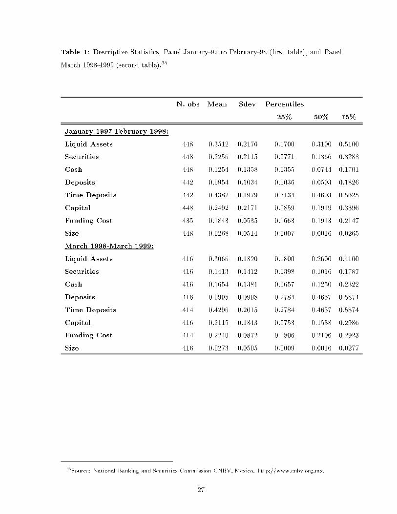
Table 1: Descriptive Statistics, Panel January-97 to February-98 (�rst table), and Panel

March 1998-1999 (second table).35

N. obs Mean Sdev Percentiles

25% 50% 75%

January 1997-February 1998:

Liquid Assets 448 0.3512 0.2176 0.1700 0.3100 0.5100

Securities 448 0.2256 0.2115 0.0771 0.1366 0.3288

Cash 448 0.1254 0.1358 0.0355 0.0744 0.1701

Deposits 442 0.0954 0.1034 0.0036 0.0503 0.1826

Time Deposits 442 0.4382 0.1979 0.3134 0.4603 0.5625

Capital 448 0.2492 0.2171 0.0859 0.1919 0.3396

Funding Cost 435 0.1843 0.0535 0.1663 0.1913 0.2147

Size 448 0.0268 0.0514 0.0007 0.0016 0.0265

March 1998-March 1999:

Liquid Assets 416 0.3066 0.1820 0.1800 0.2600 0.4100

Securities 416 0.1413 0.1412 0.0398 0.1016 0.1787

Cash 416 0.1654 0.1381 0.0657 0.1250 0.2322

Deposits 416 0.0995 0.0998 0.2784 0.4657 0.5874

Time Deposits 414 0.4296 0.2015 0.2784 0.4657 0.5874

Capital 416 0.2115 0.1843 0.0753 0.1538 0.2986

Funding Cost 414 0.2240 0.0872 0.1806 0.2106 0.2923

Size 416 0.0273 0.0505 0.0009 0.0016 0.0277

35Source: National Banking and Securities Commission CNBV, Mexico. http://www.cnbv.org.mx.

27

Table 2: Descriptive Statistics, Large Medium and Small Banks January 1997 to February 1998.36

No. obs Mean Stdev. Min Max

3 Large Banks

Liquid Assets 42 0.1829 0.0467 0.1100 0.3400

Securities 42 0.1316 0.0311 0.0760 0.2182

Cash 42 0.0512 0.0222 0.0181 0.1230

Deposits 42 0.1881 0.0375 0.1070 0.2392

Time Deposits 42 0.5006 0.0657 0.4090 0.6279

Capital 42 0.0775 0.0209 0.0451 0.1092

Funding Cost 42 0.1517 0.0289 0.1161 0.2339

Size 42 0.1729 0.0294 0.1262 0.2208

Pro�t 42 0.8078 0.0730 0.6626 0.9576

Loans 42 0.7577 0.0419 0.6056 0.8135

8 Medium Banks

Liquid Assets 112 0.2085 0.1268 0.0300 0.6000

Securities 112 0.0968 0.0571 0.0001 0.3806

Cash 112 0.1117 0.1041 0.0042 0.4932

Deposits 112 0.1912 0.1046 0.0085 0.3959

Time Deposits 112 0.4677 0.1171 0.2811 0.7106

Capital 112 0.1080 0.1084 0.0162 0.4597

Funding Cost 112 0.1727 0.0346 0.0999 0.2532

Size 112 0.0389 0.0195 0.0088 0.0757

Pro�t 112 0.8806 0.2019 0.5094 1.2643

Loans 112 0.7724 0.0978 0.4664 1.0089

21 Small Banks

Liquid Assets 294 0.4297 0.2187 0.0100 0.9000

Securities 294 0.2881 0.2352 0.0018 0.8911

Cash 294 0.1413 0.1511 0.0002 0.6939

Deposits 288 0.0446 0.0676 0.0003 0.2739

Time Deposits 288 0.4176 0.2300 0.0022 0.8894

Capital 294 0.3275 0.2222 0.0458 0.9460

Funding Cost 281 0.1938 0.0595 0.0394 0.2830

Size 294 0.0014 0.0016 0.0001 0.0077

Pro�t 288 0.7468 0.2273 0.0913 1.6051

Loans 288 0.5084 0.2165 0.0077 0.9810

36The market share to total assets is 0.51, 0.43, and 0.044 respectively. Source: CNBV (Mexico).

28

Table 3: regression results, January 1997-February 1998. *** Signi�cant at 10% con�dence

level; ** Signi�cant at 5% con�dence level; * Signi�cant at 1% con�dence level. Standard

errors in parentheses. The Hausman test tests the null hypothesis that �̂RE = �̂FE , where

�̂RE and �̂FE are the vectors of coeÆcient estimates using, respectively, the random e�ects

and the �xed e�ects regression model.

LA LA(fe) SECU SECU(fe) CASH CASH(fe)

Deposits -0.7193* -0.6268** -0.6502* -0.6517* -0.0646 0.0192

(0.1989) (0.2633) (0.2016) (0.2597) (0.1469) (0.2326)

Time Deposits 0.0832 0.0826 -0.0547 -0.0629 0.1277* 0.1440*

(0.0563) (0.0579) (0.0557) (0.0572) (0.0483) (0.0512)

Capital 0.1943** 0.1872*** 0.2750* 0.3078* -0.0487 -0.1203

(0.0892) (0.1034) (0.0896) (0.1020) (0.0695) (0.0913)

Funding Cost -0.1046 -0.0829 0.2800*** 0.2633 -0.4028* -0.3457**

(0.1583) (0.1661) (0.1569) (0.1638) (0.1351) (0.1467)

Size -0.2010 1.7391 0.2675 0.8882 -0.4957 0.8630

(0.5560) (1.6073) (0.5879) (1.5856) (0.3426) (1.4201)

No. obs 480 480 480 480 480 480

R-sq: overall 0.27 0.024 0.219 0.189 0.038 0.004

Hausman test 1.9 1.11 3.54

p-values 0.8633 0.9532 0.6172

29

Table 4: Fixed-e�ects estimates for equation (3.4) January 1997 - March 1999. Standard

errors in parentheses.

Nonperforming loans

Liquid Assets�1 -0.0148 R-sq: within 0.001

(0.0364) between 0.011

overall 0.009

Capital�1 -0.0371

(0.0803)

No. obs 484

30

Table 5: Regression results (random e�ects), January 1997-March 1999. Standard errors

in parentheses.

LA Securities Cash

Deposits (B) -0.5402 -0.4494 -0.1267

(0.1645) (0.1567) (0.1245)

Deposits (A) -0.3216 -0.2885 -0.0694

(0.1688) (0.1606) (0.1278)

Time deposits (B) 0.0600 -0.0207 0.0797

(0.0569) (0.0555) (0.0422)

Time deposits (A) 0.0406 0.0648 -0.0256

(0.0505) (0.0492) (0.0375)

Capital (B) 0.3753 0.2344 0.1456

(0.0739) (0.0717) (0.0551)

Capital (A) -0.0806 -0.0896 0.0145

(0.0729) (0.0706) (0.0544)

Funding Cost (B) -0.4940 -0.2759 -0.2021

(0.1952) (0.1903) (0.1447)

Funding Cost (A) -0.1104 0.1007 -0.2108

(0.1223) (0.1190) (0.0908)

Size (B) 0.4864 0.4446 -0.0614

(0.4538) (0.4137) (0.3587)

Size (A) 0.4598 0.5701 -0.2240

(0.4677) (0.4260) (0.3698)

No. obs 847 847 847

R-sq 0.13 0.19 0.058

Chow Test (test of equality of coeÆcients in A and B):

F-statistic 113.77 90.86 10.98

p-values 0 0 0.0518

31

Table 6: Descriptive statistics, for large, medium and small banks, March 1998 to March 1999.37

No. obs Mean Stdev. Min Max

3 Large Banks

Liquid Assets 39 0.1908 0.0452 0.1000 0.2900

Securities 39 0.1045 0.0281 0.0489 0.1661

Cash 39 0.0856 0.0377 0.0268 0.1465

Deposits 39 0.1995 0.0310 0.1429 0.2512

Time Deposits 39 0.4919 0.0685 0.3828 0.6241

Capital 39 0.0793 0.0202 0.0527 0.1144

Funding Cost 39 0.1817 0.0485 0.1202 0.2864

Size 39 0.1679 0.0333 0.1198 0.2055

Pro�t 39 0.7782 0.0720 0.6642 0.9489

Loans 39 0.7313 0.0401 0.6598 0.8093

8 Medium Banks

Liquid Assets 104 0.2939 0.1664 0.0600 0.6400

Securities 104 0.1109 0.1033 0.0001 0.4823

Cash 104 0.1830 0.1577 0.0227 0.6078

Deposits 104 0.1922 0.1052 0.0054 0.3911

Time Deposits 104 0.5014 0.1188 0.2440 0.6581

Capital 104 0.1009 0.0972 0.0323 0.4325

Funding Cost 102 0.2212 0.0647 0.1063 0.3543

Size 104 0.0424 0.0192 0.0141 0.0802

Pro�t 104 0.8529 0.2127 0.5226 1.3996

Loans 104 0.6823 0.1187 0.3676 0.9542

21 Small Banks

Liquid Assets 273 0.3280 0.1932 0.0100 0.9000

Securities 273 0.1581 0.1595 0.0001 0.7439

Cash 273 0.1701 0.1357 0.0019 0.7174

Deposits 273 0.0499 0.0607 0.0001 0.2266

Time Deposits 271 0.3931 0.2284 0.0004 0.8849

Capital 273 0.2725 0.1931 0.0270 0.9617

Funding Cost 273 0.2310 0.0967 0.0789 0.4126

Size 273 0.0015 0.0017 0.0001 0.0096

Pro�t 271 0.8173 0.1879 0.0528 1.5602

Loans 273 0.6006 0.2144 0.0069 0.9240

37The market share to total assets is 0.50, 0.45, and 0.05 respectively. Source: CNBV (Mexico).

32

Table 7: Regression results, March 1998 to March 1999. Standard errors in parentheses.

LA LA(fe) SECU SECU(fe) CASH CASH(fe)

Deposits -0.1308 0.1484 -0.0572 0.5165 -0.2489 -0.3671

(0.2008) (0.2301) (0.1697) (0.2211) (0.1455) (0.1694)

Time Deposits 0.0473 0.0401 0.1343 0.1247 -0.0875 -0.0882

(0.0557) (0.0559) (0.0523) (0.0537) (0.0399) (0.0412)

Capital -0.2803 -0.3107 -0.1916 -0.2843 -0.0346 -0.0257

(0.0810) (0.0833) (0.0744) (0.0800) (0.0581) (0.0613)

Funding Cost 0.1453 0.1256 -0.0733 -0.1007 0.2223 0.2242

(0.0785) (0.0775) (0.0754) (0.0745) (0.0561) (0.0571)

Size 0.2707 6.6671 -0.1414 6.2378 0.0939 0.3377

(0.5912) (1.4033) (0.4167) (1.3484) (0.4421) (1.0332)

No. obs 412 412 412 412 412 412

R-sq 0.07 0.12 0.08 0.16 0.06 0.07

Hausman test 35.63 50.14 3.46

p-values 0 0 0.6293

33

Figure 1: Liquid Assets and Size, January 1997-March 1999.

Panel January 1997 to March 1999.la

s ize0 .05 .1 .15 .2

0

.2

.5

.8

34

Figure 2: CoeÆcients of monthly dummy variables (for liquid assets, securities, and cash,

respectively), January 1997-March 1999.

dla

month0 6 13 20 27

-.1

-.05

0

.05

ds

ec

u

month0 6 13 20 27

-.1

-.05

0

.05

dc

as

h

month0 6 13 20 27

-.1

0

.1

.2

35

Figure 3. Average demand deposits, liquid assets, cash, and securities by bank group.

month

ldepo lal

0 6 13 20 27

.16

.18

.2

.22

.24

month

ldepo lsecu

0 6 13 20 27

.1

.15

.2

.25

month

ldepo lcash

0 6 13 20 27

.1

.15

.2

.25

month

mdepo mla

0 6 13 20 27

.15

.2

.25

.3

.35

month

mdepo msecu

0 6 13 20 27

.05

.1

.15

.2

month

mdepo mcash

0 6 13 20 27

.1

.15

.2

.25

.3

month

sdepo sla

0 6 13 20 27

0

.2

.4

.6

month

sdepo ssecu

0 6 13 20 27

0

.1

.2

.3

.4

month

sdepo scash

0 6 13 20 27

0

.1

.2

36

Figure 4. Average capital, liquid assets, cash, and securities by bank group.

month

lk lla

0 6 13 20 27

.05

.1

.15

.2

.25

month

lk lsecu

0 6 13 20 27

.05

.1

.15

.2

month

lk lcash

0 6 13 20 27

.05

.1

.15

.2

month

mk mla

0 6 13 20 27

.1

.2

.3

.4

month

mk msecu

0 6 13 20 27

.08

.1

.12

.14

month

mk mcash

0 6 13 20 27

.1

.15

.2

.25

.3

month

sk sla

0 6 13 20 27

.2

.3

.4

.5

month

sk ssecu

0 6 13 20 27

.1

.2

.3

.4

month

sk scash

0 6 13 20 27

.1

.2

.3

.4

37

References

Alger, G., \A Welfare Analysis of the Interbank Market," mimeo, GREMAQ, Universit�e

des Sciences Sociales 1999.

Bester, H. and M. Hellwig, \Moral Hazard and Equilibrium Credit Rationing: An

Overview of the Issues," in G. Bambers and K. Spremann, eds., Agency Theory Infor-

mation and Incentives, Springer Verlag 1987.

Bhattacharya, S. and D. Gale, \Preference shocks, liquidity and Central Bank pol-

icy," in W. Barnett an K. Singleton, ed., New Approaches to Monetary Economics,

Cambridge: Cambridge University Press 1987.

Edgeworth, F.Y., \The Mathematical Theory of Banking," Journal of the Royal Statis-

tical Society, 1888, pp. 113{127.

Garber, P. and S. Weisbrod, The Economics of Banking, Liquidity, and Money, Lex-

ington, MA: D.C. Heath and Company, 1992.

Hart, O. and D. Ja�ee, \On the Application of Portfolio Theory of Depository Financial

Intermediaries," Review of Economic Studies, 1974, 41, 129{147.

Hempel, G.H., D.G. Simonson, and A.B. Coleman, Bank Management: Text and

Cases (4th ed.), New York: John Wiley and Sons, 1994.

Holmstr�om, B. and J. Tirole, \Private and Public Supply of Liquidity," Journal of

Political Economy, 1998, 106, 1{40.

Kane, E.J. and B.G. Malkiel, \Bank Portfolio Allocation, Deposit Variability, and the

Availability Doctrine," Quarterly Journal of Economics, 1965, 79, 113{134.

Kashyap, A. and J. Stein, \What does a Million of Observations on Banks Say about

the Transmission of Monetary Policy?," mimeo, University of Chicago and MIT 1998.

, R. Rajan, and J. Stein, \Banks as Liquidity Providers: An Explanation for the

Co-Existence of Lending and Deposit Taking," mimeo, University of Chicago and MIT

1998.

Kyle, A., \Continuous Auctions and Insider Trading," Econometrica, 1985, 53, 1315{1335.

38

Lucas, D.J. and R.L. McDonald, \Bank Financing and Investment Decisions with

Asymmetric Information about Loan Quality," RAND Journal of Economics, 1992,

23(1), 86{105.

Marcus, A.J., \Deregulation and Bank Financial Policy," Journal of Banking and Finance,

1984, 8, 557{565.

Merton, R.C., \An Analytic Derivation of the Cost of Deposit Insurance and Loan Guar-

antees: An Application of Modern Option Pricing Theory," Journal of Banking and

Finance, 1977, 1, 3{11.

Myers, S.C. and N. Majluf, \Corporate Investment and Financing Decisions When

Firms Have Information that Investors do Not Have," Journal of Financial Economics,

1984, 13, 187{222.

Poole, W., \Commercial Bank Reserve Management in a Stochastic Model: Implications

for Monetary Policy," Journal of Finance, 1968, 23(5), 769{791.

Porter, C., \A Model of Bank Portfolio Selection," Yale Economic Essays, 1961, Fall,

323{360.

Pyle, D., \On the Theory of Financial Intermediation," Journal of Finance, 1971, 26(3),

737{747.

Rochet, J.C. and J. Tirole, \Interbank Lending and Systemic Risk," Journal of Money,

Credit and Banking, 1996, 28, 733{62.

Stiglitz, J. and J. Weiss, \Credit Rationing in Markets with Imperfect Information,"

American Economic Review, 1981, 71, 393{410.

39