Lip Reading Sentences in the Wild

Joon Son Chung1

joon@robots.ox.ac.uk

Andrew Senior2

andrewsenior@google.com

Oriol Vinyals2

vinyals@google.com

Andrew Zisserman1,2

az@robots.ox.ac.uk

1 Department of Engineering Science, University of Oxford 2 DeepMind

Abstract

The goal of this work is to recognise phrases and sen-

tences being spoken by a talking face, with or without the

audio. Unlike previous works that have focussed on recog-

nising a limited number of words or phrases, we tackle lip

reading as an open-world problem – unconstrained natural

language sentences, and in the wild videos.

Our key contributions are: (1) a ‘Watch, Listen, Attend

and Spell’ (WLAS) network that learns to transcribe videos

of mouth motion to characters; (2) a curriculum learning

strategy to accelerate training and to reduce overfitting; (3)

a ‘Lip Reading Sentences’ (LRS) dataset for visual speech

recognition, consisting of over 100,000 natural sentences

from British television.

The WLAS model trained on the LRS dataset surpasses

the performance of all previous work on standard lip read-

ing benchmark datasets, often by a significant margin. This

lip reading performance beats a professional lip reader on

videos from BBC television, and we also demonstrate that if

audio is available, then visual information helps to improve

speech recognition performance.

1. Introduction

Lip reading, the ability to recognize what is being said

from visual information alone, is an impressive skill, and

very challenging for a novice. It is inherently ambiguous

at the word level due to homophemes – different characters

that produce exactly the same lip sequence (e.g. ‘p’ and ‘b’).

However, such ambiguities can be resolved to an extent us-

ing the context of neighboring words in a sentence, and/or

a language model.

A machine that can lip read opens up a host of appli-

cations: ‘dictating’ instructions or messages to a phone in

a noisy environment; transcribing and re-dubbing archival

silent films; resolving multi-talker simultaneous speech;

and, improving the performance of automated speech

recogition in general.

That such automation is now possible is due to two de-

velopments that are well known across computer vision

tasks: the use of deep neural network models [22, 33, 35];

and, the availability of a large scale dataset for training [31].

In this case the model is based on the recent sequence-to-

sequence (encoder-decoder with attention) translater archi-

tectures that have been developed for speech recognition

and machine translation [3, 5, 15, 16, 34]. The dataset de-

veloped in this paper is based on thousands of hours of BBC

television broadcasts that have talking faces together with

subtitles of what is being said.

We also investigate how lip reading can contribute to au-

dio based speech recognition. There is a large literature on

this contribution, particularly in noisy environments, as well

as the converse where some derived measure of audio can

contribute to lip reading for the deaf or hard of hearing. To

investigate this aspect we train a model to recognize char-

acters from both audio and visual input, and then systemat-

ically disturb the audio channel or remove the visual chan-

nel.

Our model (Section 2) outputs at the character level, is

able to learn a language model, and has a novel dual at-

tention mechanism that can operate over visual input only,

audio input only, or both. We show (Section 3) that train-

ing can be accelerated by a form of curriculum learning.

We also describe (Section 4) the generation and statistics

of a new large scale Lip Reading Sentences (LRS) dataset,

based on BBC broadcasts containing talking faces together

with subtitles of what is said. The broadcasts contain faces

‘in the wild’ with a significant variety of pose, expressions,

lighting, backgrounds, and ethnic origin.

The performance of the model is assessed on a test set of

the LRS dataset, as well as on public benchmarks datasets

for lip reading including LRW [9] and GRID [11]. We

demonstrate open world (unconstrained sentences) lip read-

ing on the LRS dataset, and in all cases on public bench-

marks the performance exceeds that of prior work.

1.1. Related works

Lip reading. There is a large body of work on lip reading

using pre-deep learning methods. These methods are thor-

oughly reviewed in [40], and we will not repeat this here.

A number of papers have used Convolutional Neural Net-

16447

works (CNNs) to predict phonemes [27] or visemes [21]

from still images, as opposed recognising to full words or

sentences. A phoneme is the smallest distinguishable unit

of sound that collectively make up a spoken word; a viseme

is its visual equivalent.

For recognising full words, Petridis et al. [30] trains an

LSTM classifier on a discrete cosine transform (DCT) and

deep bottleneck features (DBF). Similarly, Wand et al. [38]

uses an LSTM with HOG input features to recognise short

phrases. The shortage of training data in lip reading pre-

sumably contributes to the continued use of shallow fea-

tures. Existing datasets consist of videos with only a small

number of subjects, and also a very limited vocabulary (<60

words), which is also an obstacle to progress. The recent

paper of Chung and Zisserman [9] tackles the small-lexicon

problem by using faces in television broadcasts to assemble

a dataset for 500 words. However, as with any word-level

classification task, the setting is still distant from the real-

world, given that the word boundaries must be known be-

forehand. A very recent work [2] uses a CNN and LSTM-

based network and Connectionist Temporal Classification

(CTC) [15] to compute the labelling. This reports strong

speaker-independent performance on the constrained gram-

mar and 51 word vocabulary of the GRID dataset [11].

However, the method, suitably modified, should be appli-

cable to longer, more general sentences.

Audio-visual speech recognition. The problems of audio-

visual speech recognition (AVSR) and lip reading are

closely linked. Mroueh et al. [26] employs feed-forward

Deep Neural Networks (DNNs) to perform phoneme classi-

fication using a large non-public audio-visual dataset. The

use of HMMs together with hand-crafted or pre-trained vi-

sual features have proved popular – [36] encodes input im-

ages using DBF; [14] used DCT; and [28] uses a CNN

pre-trained to classify phonemes; all three combine these

features with HMMs to classify spoken digits or isolated

words. As with lip reading, there has been little attempt

to develop AVSR systems that generalise to real-world set-

tings.

Speech recognition. There is a wealth of literature on

speech recognition systems that utilise separate components

for acoustic and language-modelling functions (e.g. hybrid

DNN-HMM systems), that we will not review here. We re-

strict this review to methods that can be trained end-to-end.

For the most part, prior work can be divided into two

types. The first type uses CTC [15], where the model typ-

ically predicts framewise labels and then looks for the op-

timal alignment between the framewise predictions and the

output sequence. The weakness is that the output labels are

not conditioned on each other.

The second type is sequence-to-sequence models [34]

that first read all of the input sequence before starting to pre-

dict the output sentence. A number of papers have adopted

this approach for speech recognition [7, 8], and the most re-

lated work to ours is that of Chan et al. [5] which proposes

an elegant sequence-to-sequence method to transcribe au-

dio signal to characters. They utilise a number of the latest

sequence learning tricks such as scheduled sampling [4] and

attention [8]; we take many inspirations from this work.

2. Architecture

In this section, we describe the Watch, Listen, Attend and

Spell network that learns to predict characters in sentences

being spoken from a video of a talking face, with or without

audio.

We model each character yi in the output character se-

quence y = (y1, y2, ..., yl) as a conditional distribution

of the previous characters y<i, the input image sequence

xv = (xv

1, xv2, ..., x

vn) for lip reading, and the input audio

sequence xa = (xa

1 , xa2 , ..., x

am). Hence, we model the out-

put probability distribution as:

P (y|xv,xa) =∏

i

P (yi|xv,xa, y<i) (1)

Our model, which is summarised in Figure 1, con-

sists of three key components: the image encoder Watch

(Section 2.1), the audio encoder Listen (Section 2.2),

and the character decoder Spell (Section 2.3). Each en-

coder transforms the respective input sequence into a fixed-

dimensional state vector s, and sequences of encoder out-

puts o = (o1, ..., op), p ∈ (n,m); the decoder ingests the

state and the attention vectors from both encoders and pro-

duces a probability distribution over the output character se-

quence.

sv,ov = Watch(xv) (2)

sa,oa = Listen(xa) (3)

P (y|xv,xa) = Spell(sv, sa,ov,oa) (4)

The three modules in the model are trained jointly. We

describe the modules next, with implementation details

given in Section 3.5.

2.1. Watch: Image encoder

The image encoder consists of the convolutional module

that generates image features fvi for every input timestep

xvi , and the recurrent module that produces the fixed-

dimensional state vector sv and a set of output vectors ov .

fvi = CNN(xv

i ) (5)

hvi , o

vi = LSTM(fv

i , hvi+1) (6)

sv = hv1 (7)

The convolutional network is based on the VGG-M

model [6], as it is memory-efficient, fast to train and has

a decent classification performance on ImageNet [31]. The

6448

LSTMLSTMLSTMLSTMLSTMLSTM

fc6...

conv1

fc6...

conv1

fc6...

conv1

fc6...

conv1

fc6...

conv1

fc6...

conv1

LSTM LSTM LSTM LSTM LSTM

LSTMLSTMLSTMLSTMLSTMLSTMLSTMLSTM

mfcc1mfcc2mfcc3mfcc4mfcc5mfcc6mfcc7mfcc8

att att att att attatt att att att att

MLP MLP MLP MLP MLP

output states vid

output states aud

y1 y2 y3 y4 (end)

(start) y1 y2 y3 y4

ov

oa

sa

sv

Figure 1. Watch, Listen, Attend and Spell architecture. At each time step, the decoder outputs a character yi, as well as two attention

vectors. The attention vectors are used to select the appropriate period of the input visual and audio sequences.

input (120x120) conv1 conv2 conv3 conv4 conv5 fc6

596 256

512 512512

512

convmaxnorm

convmaxnorm

conv conv convmax

full

33

33

33 3

33

3

Figure 2. The ConvNet architecture. The input is five gray level frames centered on the mouth region. The 512-dimensional fc6 vector

forms the input to the LSTM.

ConvNet layer configuration is shown in Figure 2, and is

abbreviated as conv1 · · · fc6 in the main network diagram.

The encoder LSTM network consumes the output fea-

tures fvi produced by the ConvNet at every input timestep,

and generates a fixed-dimensional state vector sv . In ad-

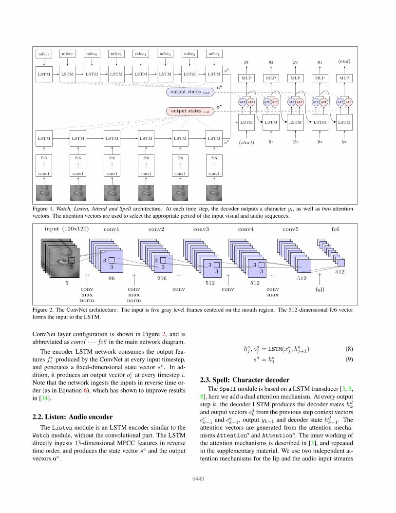
dition, it produces an output vector ovi at every timestep i.Note that the network ingests the inputs in reverse time or-

der (as in Equation 6), which has shown to improve results

in [34].

2.2. Listen: Audio encoder

The Listen module is an LSTM encoder similar to the

Watch module, without the convolutional part. The LSTM

directly ingests 13-dimensional MFCC features in reverse

time order, and produces the state vector sa and the output

vectors oa.

haj , o

aj = LSTM(xa

j , haj+1) (8)

sa = ha1 (9)

2.3. Spell: Character decoder

The Spell module is based on a LSTM transducer [3, 5,

8], here we add a dual attention mechanism. At every output

step k, the decoder LSTM produces the decoder states hdk

and output vectors odk from the previous step context vectors

cvk−1 and cak−1, output yk−1 and decoder state hdk−1. The

attention vectors are generated from the attention mecha-

nisms Attentionv and Attentiona. The inner working of

the attention mechanisms is described in [3], and repeated

in the supplementary material. We use two independent at-

tention mechanisms for the lip and the audio input streams

6449

to refer to the asynchronous inputs with different sampling

rates. The attention vectors are fused with the output states

(Equations 11 and 12) to produce the context vectors cvk and

cak that encapsulate the information required to produce the

next step output. The probability distribution of the output

character is generated by an MLP with softmax over the

output.

hdk, o

dk = LSTM(hd

k−1, yk−1, cvk−1, c

ak−1) (10)

cvk = ov · Attentionv(hd

k,ov) (11)

cak = oa · Attentiona(hd

k,oa) (12)

P (yi|xv,xa, y<i) = softmax(MLP(odk, c

vk, c

ak)) (13)

At k = 1, the final encoder states sl and sa are used as

the input instead of the previous decoder state – i.e. hd0 =

concat(sa, sv) – to help produce the context vectors cv1 and

ca1 in the absence of the previous state or context.

Discussion. In our experiments, we have observed that

the attention mechanism is absolutely critical for the audio-

visual speech recognition system to work. Without atten-

tion, the model appears to ‘forget’ the input signal, and pro-

duces an output sequence that correlates very little to the

input, beyond the first word or two (which the model gets

correct, as these are the last words to be seen by the en-

coder). The attention-less model yields Word Error Rates

over 100%, so we do not report these results.

The dual-attention mechanism allows the model to ex-

tract information from both audio and video inputs, even

when one stream is absent, or the two streams are not time-

aligned. The benefits are clear in the experiments with noisy

or no audio (Section 5).

Bidirectional LSTMs have been used in many sequence

learning tasks [5, 8, 17] for their ability to produce out-

puts conditioned on future context as well as past con-

text. We have tried replacing the unidirectional encoders

in the Watch and Listen modules with bidirectional en-

coders, however these networks took significantly longer

to train, whilst providing no obvious performance improve-

ment. This is presumably because the Decoder module is

anyway conditioned on the full input sequence, so bidirec-

tional encoders are not necessary for providing context, and

the attention mechanism suffices to provide the additional

local focus.

3. Training strategy

In this section, we describe the strategy used to effec-

tively train the Watch, Listen, Attend and Spell network,

making best use of the limited amount of data available.

3.1. Curriculum learning

Our baseline strategy is to train the model from scratch,

using the full sentences from the ‘Lip Reading Sentences’

dataset – previous works in speech recognition have taken

this approach. However, as [5] reports, the LSTM net-

work converges very slowly when the number of timesteps

is large, because the decoder initially has a hard time ex-

tracting the relevant information from all the input steps.

We introduce a new strategy where we start training only

on single word examples, and then let the sequence length

grow as the network trains. These short sequences are parts

of the longer sentences in the dataset. We observe that the

rate of convergence on the training set is several times faster,

and it also significantly reduces overfitting, presumably be-

cause it works as a natural way of augmenting the data. The

test performance improves by a large margin, reported in

Section 5.

3.2. Scheduled sampling

When training a recurrent neural network, one typically

uses the previous time step ground truth as the next time

step input, which helps the model learn a kind of lan-

guage model over target tokens. However during inference,

the previous step ground-truth is unavailable, resulting in

poorer performance because the model was not trained to

be tolerant to feeding in bad predictions at some time steps.

We use the scheduled sampling method of Bengio et al. [4]

to bridge this discrepancy between how the model is used

at training and inference. At train time, we randomly

sample from the previous output, instead of always using

the ground-truth. When training on shorter sub-sequences,

ground-truth previous characters are used. When training

on full sentences, the sampling probability from the previ-

ous output was increased in steps from 0 to 0.25 over time.

We were not able to achieve stable learning at sampling

probabilities of greater than 0.25.

3.3. Multi­modal training

Networks with multi-modal inputs can often be domi-

nated by one of the modes [13]. In our case we observe that

the audio signal dominates, because speech recognition is a

significantly easier problem than lip reading. To help pre-

vent this from happening, one of the following input types is

uniformly selected at train time for each example: (1) audio

only; (2) lips only; (3) audio and lips.

If mode (1) is selected, the audio-only data described in

Section 4.1 is used. Otherwise, the standard audio-visual

data is used.

We have over 300,000 sentences in the recorded data,

but only around 100,000 have corresponding facetracks. In

machine translation, it has been shown that monolingual

dummy data can be used to help improve the performance

of a translation model [32]. By similar rationale, we use the

sentences without facetracks as supplementary training data

to boost audio recognition performance and to build a richer

language model to help improve generalisation.

6450

3.4. Training with noisy audio

The WLAS model is initially trained with clean input

audio for faster convergence. To improve the model’s toler-

ance to audio noise, we apply additive white Gaussian noise

with SNR of 10dB (10:1 ratio of the signal power to the

noise power) and 0dB (1:1 ratio) later in training.

3.5. Implementation details

The input images are 120×120 in dimension, and are

sampled at 25Hz. The image only covers the lip region of

the face, as shown in Figure 3. The ConvNet ingests 5-

frame sliding windows using the Early Fusion method of

[9], moving 1-frame at a time. The MFCC features are

calculated over 25ms windows and at 100Hz, with a time-

stride of 1. For Watch and Listen modules, we use a three

layer LSTM with cell size of 256. For the Spell mod-

ule, we use a three layer LSTM with cell size of 512. The

output size of the network is 45, for every character in the

alphabet, numbers, common punctuations, and tokens for

[sos], [eos], [pad]. The full list is given in the sup-

plementary material.

Our implementation is based on the TensorFlow li-

brary [1] and trained on a GeForce Titan X GPU with 12GB

memory. The network is trained using stochastic gradient

descent with a batch size of 64 and with dropout and la-

bel smoothing. The layer weights of the convolutional lay-

ers are initialised from the visual stream of [10]. All other

weights are randomly initialised.

An initial learning rate of 0.1 was used, and decreased by

10% every time the training error did not improve for 2,000

iterations. Training on the full sentence data was stopped

when the validation error did not improve for 5,000 itera-

tions. The model was trained for around 500,000 iterations,

which took approximately 10 days.

4. Dataset

In this section, we describe the multi-stage pipeline for

automatically generating a large-scale dataset for audio-

visual speech recognition. Using this pipeline, we have

been able to collect thousands of hours of spoken sentences

and phrases along with the corresponding facetrack. We

use a variety of BBC programs recorded between 2010 and

2016, listed in Table 1, and shown in Figure 3.

The selection of programs are deliberately similar to

those used by [9] for two reasons: (1) a wide range of

speakers appear in the news and the debate programs, un-

like dramas with a fixed cast; (2) shot changes are less fre-

quent, therefore there are more full sentences with continu-

ous facetracks.

The processing pipeline is summarised in Figure 4. Most

of the steps are based on the methods described in [9] and

[10], but we give a brief sketch of the method here.

Video preparation. First, shot boundaries are de-

Channel Series name # hours # sent.

BBC 1 HD News† 1,584 50,493

BBC 1 HD Breakfast 1,997 29,862

BBC 1 HD Newsnight 590 17,004

BBC 2 HD World News 194 3,504

BBC 2 HD Question Time 323 11,695

BBC 4 HD World Today 272 5,558

All 4,960 118,116

Table 1. Video statistics. The number of hours of the original BBC

video; the number of sentences with full facetrack. †BBC News at

1, 6 and 10.

tected by comparing colour histograms across consecutive

frames [24]. The HOG-based face detection [20] is then

performed on every frame of the video. The face detections

of the same person are grouped across frames using a KLT

tracker [37]. Facial landmarks are extracted from a sparse

subset of pixel intensities using an ensemble of regression

trees [19].

Audio and text preparation. The subtitles in BBC videos

are not broadcast in sync with the audio. The Penn Phonet-

ics Lab Forced Aligner [18, 39] is used to force-align the

subtitle to the audio signal. Errors exist in the alignment

as the transcript is not verbatim – therefore the aligned la-

bels are filtered by checking against the commercial IBM

Watson Speech to Text service.

AV sync and speaker detection. In BBC videos, the audio

and the video streams can be out of sync by up to around

one second, which can cause problems when the facetrack

corresponding to a sentence is being extracted. The two-

stream network described in [10] is used to synchronise the

two streams. The same network is also used to determine

who is speaking in the video, and reject the clip if it is a

voice-over.

Sentence extraction. The videos are divided into invidid-

ual sentences/ phrases using the punctuations in the tran-

script. The sentences are separated by full stops, commas

and question marks; and are clipped to 100 characters or

10 seconds, due to GPU memory constraints. We do not

impose any restrictions on the vocabulary size.

The training, validation and test sets are divided accord-

ing to broadcast date, and the dates of videos corresponding

to each set are shown in Table 2. The dataset contains thou-

sands of different speakers which enables the model to be

speaker agnostic.

Table 3 compares the ‘Lip Reading Sentences’ (LRS)

dataset to the largest existing public datasets.

4.1. Audio­only data

In addition to the audio-visual dataset, we prepare an

auxiliary audio-only training dataset. These are the sen-

tences in the BBC programs for which facetracks are not

available. The use of this data is described in Section 3.3. It

is only used for training, not for testing.

6451

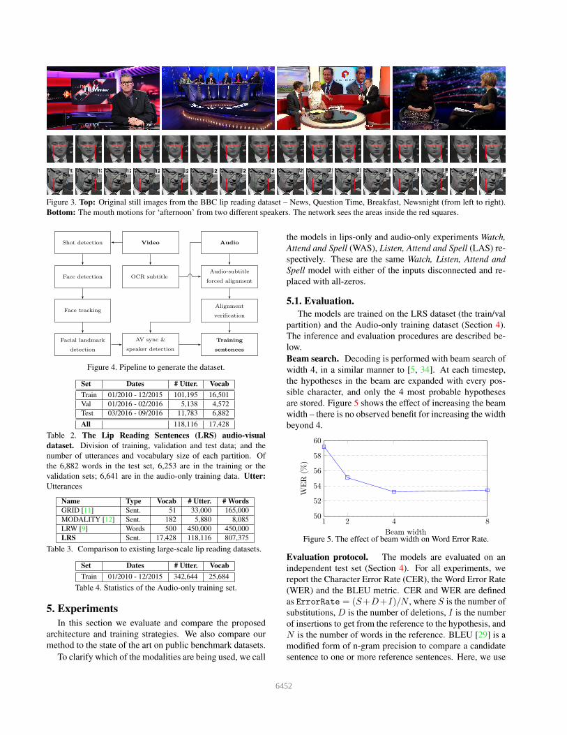
Figure 3. Top: Original still images from the BBC lip reading dataset – News, Question Time, Breakfast, Newsnight (from left to right).

Bottom: The mouth motions for ‘afternoon’ from two different speakers. The network sees the areas inside the red squares.

Audio

Audio-subtitle

forced alignment

Alignment

verification

Video

OCR subtitle

Shot detection

Face detection

Face tracking

Facial landmark

detection

AV sync &

speaker detection

Training

sentences

Figure 4. Pipeline to generate the dataset.

Set Dates # Utter. Vocab

Train 01/2010 - 12/2015 101,195 16,501

Val 01/2016 - 02/2016 5,138 4,572

Test 03/2016 - 09/2016 11,783 6,882

All 118,116 17,428

Table 2. The Lip Reading Sentences (LRS) audio-visual

dataset. Division of training, validation and test data; and the

number of utterances and vocabulary size of each partition. Of

the 6,882 words in the test set, 6,253 are in the training or the

validation sets; 6,641 are in the audio-only training data. Utter:

Utterances

Name Type Vocab # Utter. # Words

GRID [11] Sent. 51 33,000 165,000

MODALITY [12] Sent. 182 5,880 8,085

LRW [9] Words 500 450,000 450,000

LRS Sent. 17,428 118,116 807,375

Table 3. Comparison to existing large-scale lip reading datasets.

Set Dates # Utter. Vocab

Train 01/2010 - 12/2015 342,644 25,684

Table 4. Statistics of the Audio-only training set.

5. Experiments

In this section we evaluate and compare the proposed

architecture and training strategies. We also compare our

method to the state of the art on public benchmark datasets.

To clarify which of the modalities are being used, we call

the models in lips-only and audio-only experiments Watch,

Attend and Spell (WAS), Listen, Attend and Spell (LAS) re-

spectively. These are the same Watch, Listen, Attend and

Spell model with either of the inputs disconnected and re-

placed with all-zeros.

5.1. Evaluation.

The models are trained on the LRS dataset (the train/val

partition) and the Audio-only training dataset (Section 4).

The inference and evaluation procedures are described be-

low.

Beam search. Decoding is performed with beam search of

width 4, in a similar manner to [5, 34]. At each timestep,

the hypotheses in the beam are expanded with every pos-

sible character, and only the 4 most probable hypotheses

are stored. Figure 5 shows the effect of increasing the beam

width – there is no observed benefit for increasing the width

beyond 4.

1 2 4 850

52

54

56

58

60

Beam width

WER

(%)

Figure 5. The effect of beam width on Word Error Rate.

Evaluation protocol. The models are evaluated on an

independent test set (Section 4). For all experiments, we

report the Character Error Rate (CER), the Word Error Rate

(WER) and the BLEU metric. CER and WER are defined

as ErrorRate = (S+D+I)/N , where S is the number of

substitutions, D is the number of deletions, I is the number

of insertions to get from the reference to the hypothesis, and

N is the number of words in the reference. BLEU [29] is a

modified form of n-gram precision to compare a candidate

sentence to one or more reference sentences. Here, we use

6452

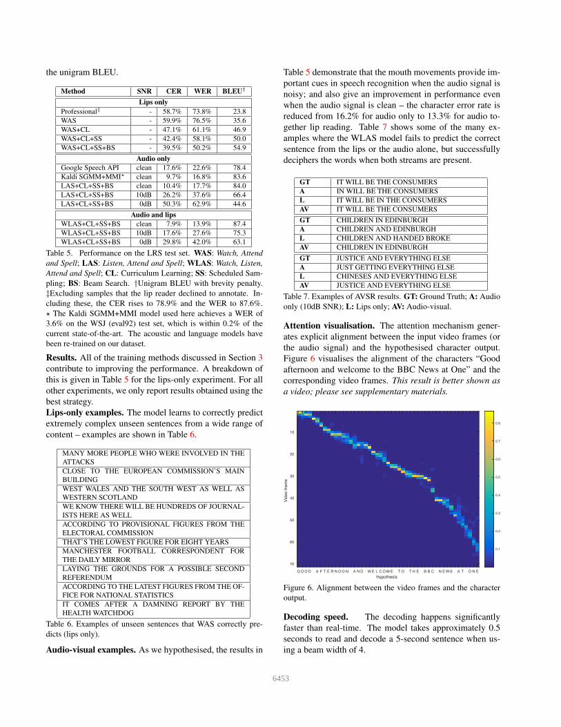
the unigram BLEU.

Method SNR CER WER BLEU†

Lips only

Professional‡ - 58.7% 73.8% 23.8

WAS - 59.9% 76.5% 35.6

WAS+CL - 47.1% 61.1% 46.9

WAS+CL+SS - 42.4% 58.1% 50.0

WAS+CL+SS+BS - 39.5% 50.2% 54.9

Audio only

Google Speech API clean 17.6% 22.6% 78.4

Kaldi SGMM+MMI⋆ clean 9.7% 16.8% 83.6

LAS+CL+SS+BS clean 10.4% 17.7% 84.0

LAS+CL+SS+BS 10dB 26.2% 37.6% 66.4

LAS+CL+SS+BS 0dB 50.3% 62.9% 44.6

Audio and lips

WLAS+CL+SS+BS clean 7.9% 13.9% 87.4

WLAS+CL+SS+BS 10dB 17.6% 27.6% 75.3

WLAS+CL+SS+BS 0dB 29.8% 42.0% 63.1

Table 5. Performance on the LRS test set. WAS: Watch, Attend

and Spell; LAS: Listen, Attend and Spell; WLAS: Watch, Listen,

Attend and Spell; CL: Curriculum Learning; SS: Scheduled Sam-

pling; BS: Beam Search. †Unigram BLEU with brevity penalty.

‡Excluding samples that the lip reader declined to annotate. In-

cluding these, the CER rises to 78.9% and the WER to 87.6%.

⋆ The Kaldi SGMM+MMI model used here achieves a WER of

3.6% on the WSJ (eval92) test set, which is within 0.2% of the

current state-of-the-art. The acoustic and language models have

been re-trained on our dataset.

Results. All of the training methods discussed in Section 3

contribute to improving the performance. A breakdown of

this is given in Table 5 for the lips-only experiment. For all

other experiments, we only report results obtained using the

best strategy.

Lips-only examples. The model learns to correctly predict

extremely complex unseen sentences from a wide range of

content – examples are shown in Table 6.

MANY MORE PEOPLE WHO WERE INVOLVED IN THE

ATTACKS

CLOSE TO THE EUROPEAN COMMISSION’S MAIN

BUILDING

WEST WALES AND THE SOUTH WEST AS WELL AS

WESTERN SCOTLAND

WE KNOW THERE WILL BE HUNDREDS OF JOURNAL-

ISTS HERE AS WELL

ACCORDING TO PROVISIONAL FIGURES FROM THE

ELECTORAL COMMISSION

THAT’S THE LOWEST FIGURE FOR EIGHT YEARS

MANCHESTER FOOTBALL CORRESPONDENT FOR

THE DAILY MIRROR

LAYING THE GROUNDS FOR A POSSIBLE SECOND

REFERENDUM

ACCORDING TO THE LATEST FIGURES FROM THE OF-

FICE FOR NATIONAL STATISTICS

IT COMES AFTER A DAMNING REPORT BY THE

HEALTH WATCHDOG

Table 6. Examples of unseen sentences that WAS correctly pre-

dicts (lips only).

Audio-visual examples. As we hypothesised, the results in

Table 5 demonstrate that the mouth movements provide im-

portant cues in speech recognition when the audio signal is

noisy; and also give an improvement in performance even

when the audio signal is clean – the character error rate is

reduced from 16.2% for audio only to 13.3% for audio to-

gether lip reading. Table 7 shows some of the many ex-

amples where the WLAS model fails to predict the correct

sentence from the lips or the audio alone, but successfully

deciphers the words when both streams are present.

GT IT WILL BE THE CONSUMERS

A IN WILL BE THE CONSUMERS

L IT WILL BE IN THE CONSUMERS

AV IT WILL BE THE CONSUMERS

GT CHILDREN IN EDINBURGH

A CHILDREN AND EDINBURGH

L CHILDREN AND HANDED BROKE

AV CHILDREN IN EDINBURGH

GT JUSTICE AND EVERYTHING ELSE

A JUST GETTING EVERYTHING ELSE

L CHINESES AND EVERYTHING ELSE

AV JUSTICE AND EVERYTHING ELSE

Table 7. Examples of AVSR results. GT: Ground Truth; A: Audio

only (10dB SNR); L: Lips only; AV: Audio-visual.

Attention visualisation. The attention mechanism gener-

ates explicit alignment between the input video frames (or

the audio signal) and the hypothesised character output.

Figure 6 visualises the alignment of the characters “Good

afternoon and welcome to the BBC News at One” and the

corresponding video frames. This result is better shown as

a video; please see supplementary materials.

Hypothesis

G O O D A F T E R N O O N A N D W E L C O M E T O T H E B B C N E W S A T O N E

Vid

eo fra

me

10

20

30

40

50

60

70

0.1

0.2

0.3

0.4

0.5

0.6

0.7

0.8

Figure 6. Alignment between the video frames and the character

output.

Decoding speed. The decoding happens significantly

faster than real-time. The model takes approximately 0.5

seconds to read and decode a 5-second sentence when us-

ing a beam width of 4.

6453

5.2. Human experiment

In order to compare the performance of our model to

what a human can achieve, we instructed a professional

lip reading company to decipher a random sample of 200

videos from our test set. The lip reader has around 10 years

of professional experience and deciphered videos in a range

of settings, e.g. forensic lip reading for use in court, the

royal wedding, etc.

The lip reader was allowed to see the full face (the whole

picture in the bottom two rows of Figure 3), but not the

background, in order to prevent them from reading subtitles

or guessing the words from the video content. However,

they were informed which program the video comes from,

and were allowed to look at some videos from the training

set with ground truth.

The lip reader was given 10 times the video duration to

predict the words being spoken, and within that time, they

were allowed to watch the video as many times as they

wished. Each of the test sentences was up to 100 charac-

ters in length.

We observed that the professional lip reader is able to

correctly decipher less than one-quarter of the spoken words

(Table 5). This is consistent with previous studies on the

accuracy of human lip reading [25]. In contrast, the WAS

model (lips only) is able to decipher half of the spoken

words. Thus, this is significantly better than professional

lip readers can achieve.

5.3. LRW dataset

The ‘Lip Reading in the Wild’ (LRW) dataset consists

of up to 1000 utterances of 500 isolated words from BBC

television, spoken by over a thousand different speakers.

Evaluation protocol. The train, validation and test splits

are provided with the dataset. We give word error rates.

Results. The network is fine-tuned for one epoch to clas-

sify only the 500 word classes of this dataset’s lexicon. As

shown in Table 8, our result exceeds the current state-of-

the-art on this dataset by a large margin.

Methods LRW [9] GRID [11]

Lan et al. [23] - 35.0%

Wand et al. [38] - 20.4%

Assael et al. [2] - 4.8%

Chung and Zisserman [9] 38.9% -

WAS (ours) 23.8% 3.0%

Table 8. Word error rates on external lip reading datasets.

5.4. GRID dataset

The GRID dataset [11] consists of 34 subjects, each

uttering 1000 phrases. The utterances are single-syntax

multi-word sequences of verb (4) + color (4) +

preposition (4) + alphabet (25) + digit (10) +

adverb (4) ; e.g. ‘put blue at A 1 now’. The total vocab-

ulary size is 51, but the number of possibilities at any given

Figure 7. Still images from the GRID dataset.

point in the output is effectively constrained to the numbers

in the brackets above. The videos are recorded in a con-

trolled lab environment, shown in Figure 7.

Evaluation protocol. The evaluation follows the standard

protocol of [38] and [2] – the data is randomly divided into

train, validation and test sets, where the latter contains 255

utterances for each speaker. We report the word error rates.

Some of the previous works report word accuracies, which

is defined as (WAcc = 1− WER).

Results. The network is fine-tuned for one epoch on the

GRID dataset training set. As can be seen in Table 8, our

method achieves a strong performance of 3.0% (WER), that

substantially exceeds the current state-of-the-art.

6. Summary and extensions

In this paper, we have introduced the ‘Watch, Listen, At-

tend and Spell’ network model that can transcribe speech

into characters. The model utilises a novel dual attention

mechanism that can operate over visual input only, audio

input only, or both. Using this architecture, we demonstrate

lip reading performance that beats a professional lip reader

on videos from BBC television. The model also surpasses

the performance of all previous work on standard lip read-

ing benchmark datasets, and we also demonstrate that vi-

sual information helps to improve speech recognition per-

formance even when the audio is used.

There are several interesting extensions to consider:

first, the attention mechanism that provides the alignment

is unconstrained, but in practice should always move

monotonically from left to right. This monotonicity could

be incorporated as a soft or hard constraint; second, the

sequence-to-sequence model is used in batch mode –

decoding a sentence given the entire corresponding lip se-

quence. Instead, a more on-line architecture could be used,

where the decoder does not have access to the part of the lip

sequence in the future; finally, it is possible that research of

this type could discern important discriminative cues that

are beneficial for teaching lip reading to the hard of hearing.

Acknowledgements. Funding for this research is provided

by the EPSRC Programme Grant Seebibyte EP/M013774/1.

We are very grateful to Rob Cooper and Matt Haynes at

BBC Research for help in obtaining the dataset at Oxford.

6454

References

[1] M. Abadi, A. Agarwal, P. Barham, E. Brevdo, Z. Chen,

C. Citro, G. S. Corrado, A. Davis, J. Dean, M. Devin, et al.

Tensorflow: Large-scale machine learning on heterogeneous

distributed systems. arXiv preprint arXiv:1603.04467, 2016.

5[2] Y. M. Assael, B. Shillingford, S. Whiteson, and N. de Freitas.

Lipnet: Sentence-level lipreading. arXiv:1611.01599, 2016.

2, 8[3] D. Bahdanau, K. Cho, and Y. Bengio. Neural machine trans-

lation by jointly learning to align and translate. Proc. ICLR,

2015. 1, 3[4] S. Bengio, O. Vinyals, N. Jaitly, and N. Shazeer. Scheduled

sampling for sequence prediction with recurrent neural net-

works. In Advances in Neural Information Processing Sys-

tems, pages 1171–1179, 2015. 2, 4[5] W. Chan, N. Jaitly, Q. V. Le, and O. Vinyals. Listen, attend

and spell. arXiv preprint arXiv:1508.01211, 2015. 1, 2, 3, 4,

6[6] K. Chatfield, K. Simonyan, A. Vedaldi, and A. Zisserman.

Return of the devil in the details: Delving deep into convo-

lutional nets. In Proc. BMVC., 2014. 2[7] J. Chorowski, D. Bahdanau, K. Cho, and Y. Bengio. End-

to-end continuous speech recognition using attention-based

recurrent nn: first results. arXiv preprint arXiv:1412.1602,

2014. 2[8] J. K. Chorowski, D. Bahdanau, D. Serdyuk, K. Cho, and

Y. Bengio. Attention-based models for speech recogni-

tion. In Advances in Neural Information Processing Systems,

pages 577–585, 2015. 2, 3, 4[9] J. S. Chung and A. Zisserman. Lip reading in the wild. In

Proc. ACCV, 2016. 1, 2, 5, 6, 8[10] J. S. Chung and A. Zisserman. Out of time: automated lip

sync in the wild. In Workshop on Multi-view Lip-reading,

ACCV, 2016. 5[11] M. Cooke, J. Barker, S. Cunningham, and X. Shao. An

audio-visual corpus for speech perception and automatic

speech recognition. The Journal of the Acoustical Society

of America, 120(5):2421–2424, 2006. 1, 2, 6, 8[12] A. Czyzewski, B. Kostek, P. Bratoszewski, J. Kotus, and

M. Szykulski. An audio-visual corpus for multimodal auto-

matic speech recognition. Journal of Intelligent Information

Systems, pages 1–26, 2017. 6[13] C. Feichtenhofer, A. Pinz, and A. Zisserman. Convolutional

two-stream network fusion for video action recognition. In

Proc. CVPR, 2016. 4[14] G. Galatas, G. Potamianos, and F. Makedon. Audio-visual

speech recognition incorporating facial depth information

captured by the kinect. In Signal Processing Conference

(EUSIPCO), 2012 Proceedings of the 20th European, pages

2714–2717. IEEE, 2012. 2[15] A. Graves, S. Fernandez, F. Gomez, and J. Schmidhu-

ber. Connectionist temporal classification: labelling unseg-

mented sequence data with recurrent neural networks. In

Proceedings of the 23rd international conference on Ma-

chine learning, pages 369–376. ACM, 2006. 1, 2[16] A. Graves and N. Jaitly. Towards end-to-end speech recog-

nition with recurrent neural networks. In Proceedings of the

31st International Conference on Machine Learning (ICML-

14), pages 1764–1772, 2014. 1[17] A. Graves, N. Jaitly, and A.-r. Mohamed. Hybrid speech

recognition with deep bidirectional LSTM. In Automatic

Speech Recognition and Understanding (ASRU), 2013 IEEE

Workshop on, pages 273–278. IEEE, 2013. 4[18] H. Hermansky. Perceptual linear predictive (PLP) analysis

of speech. the Journal of the Acoustical Society of America,

87(4):1738–1752, 1990. 5[19] V. Kazemi and J. Sullivan. One millisecond face alignment

with an ensemble of regression trees. In Proceedings of the

IEEE Conference on Computer Vision and Pattern Recogni-

tion, pages 1867–1874, 2014. 5[20] D. E. King. Dlib-ml: A machine learning toolkit. The Jour-

nal of Machine Learning Research, 10:1755–1758, 2009. 5[21] O. Koller, H. Ney, and R. Bowden. Deep learning of mouth

shapes for sign language. In Proceedings of the IEEE Inter-

national Conference on Computer Vision Workshops, pages

85–91, 2015. 2[22] A. Krizhevsky, I. Sutskever, and G. E. Hinton. ImageNet

classification with deep convolutional neural networks. In

NIPS, pages 1106–1114, 2012. 1[23] Y. Lan, R. Harvey, B. Theobald, E.-J. Ong, and R. Bow-

den. Comparing visual features for lipreading. In Inter-

national Conference on Auditory-Visual Speech Processing

2009, pages 102–106, 2009. 8[24] R. Lienhart. Reliable transition detection in videos: A survey

and practitioner’s guide. International Journal of Image and

Graphics, Aug 2001. 5[25] M. Marschark and P. E. Spencer. The Oxford handbook of

deaf studies, language, and education, volume 2. Oxford

University Press, 2010. 8[26] Y. Mroueh, E. Marcheret, and V. Goel. Deep multimodal

learning for audio-visual speech recognition. In 2015 IEEE

International Conference on Acoustics, Speech and Signal

Processing (ICASSP), pages 2130–2134. IEEE, 2015. 2[27] K. Noda, Y. Yamaguchi, K. Nakadai, H. G. Okuno, and

T. Ogata. Lipreading using convolutional neural network.

In INTERSPEECH, pages 1149–1153, 2014. 2[28] K. Noda, Y. Yamaguchi, K. Nakadai, H. G. Okuno, and

T. Ogata. Audio-visual speech recognition using deep learn-

ing. Applied Intelligence, 42(4):722–737, 2015. 2[29] K. Papineni, S. Roukos, T. Ward, and W.-J. Zhu. Bleu: a

method for automatic evaluation of machine translation. In

Proceedings of the 40th annual meeting on association for

computational linguistics, pages 311–318. Association for

Computational Linguistics, 2002. 6[30] S. Petridis and M. Pantic. Deep complementary bottleneck

features for visual speech recognition. ICASSP, pages 2304–

2308, 2016. 2[31] O. Russakovsky, J. Deng, H. Su, J. Krause, S. Satheesh,

S. Ma, S. Huang, A. Karpathy, A. Khosla, M. Bernstein,

A. Berg, and F. Li. ImageNet Large Scale Visual Recog-

nition Challenge. IJCV, 2015. 1, 2[32] R. Sennrich, B. Haddow, and A. Birch. Improving neural

machine translation models with monolingual data. arXiv

preprint arXiv:1511.06709, 2015. 4[33] K. Simonyan and A. Zisserman. Very deep convolutional

networks for large-scale image recognition. In International

Conference on Learning Representations, 2015. 1[34] I. Sutskever, O. Vinyals, and Q. Le. Sequence to sequence

6455

learning with neural networks. In Advances in neural infor-

mation processing systems, pages 3104–3112, 2014. 1, 2, 3,

6[35] C. Szegedy, W. Liu, Y. Jia, P. Sermanet, S. Reed,

D. Anguelov, D. Erhan, V. Vanhoucke, and A. Rabinovich.

Going deeper with convolutions. In Proc. CVPR, 2015. 1[36] S. Tamura, H. Ninomiya, N. Kitaoka, S. Osuga, Y. Iribe,

K. Takeda, and S. Hayamizu. Audio-visual speech recog-

nition using deep bottleneck features and high-performance

lipreading. In 2015 Asia-Pacific Signal and Information Pro-

cessing Association Annual Summit and Conference (AP-

SIPA), pages 575–582. IEEE, 2015. 2[37] C. Tomasi and T. Kanade. Selecting and tracking features for

image sequence analysis. Robotics and Automation, 1992. 5[38] M. Wand, J. Koutn, et al. Lipreading with long short-term

memory. In 2016 IEEE International Conference on Acous-

tics, Speech and Signal Processing (ICASSP), pages 6115–

6119. IEEE, 2016. 2, 8[39] J. Yuan and M. Liberman. Speaker identification on the sco-

tus corpus. Journal of the Acoustical Society of America,

123(5):3878, 2008. 5[40] Z. Zhou, G. Zhao, X. Hong, and M. Pietikainen. A review of

recent advances in visual speech decoding. Image and vision

computing, 32(9):590–605, 2014. 1

6456