Linköping University Post Print

Combining shadow detection and simulation

for estimation of vehicle size and position

Björn Johansson, Johan Wiklund, Per-Erik Forssén and Gösta Granlund

N.B.: When citing this work, cite the original article.

Original Publication:

Björn Johansson, Johan Wiklund, Per-Erik Forssén and Gösta Granlund, Combining shadow

detection and simulation for estimation of vehicle size and position, 2009, PATTERN

RECOGNITION LETTERS, (30), 8, 751-759.

http://dx.doi.org/10.1016/j.patrec.2009.03.005

Copyright: Elsevier Science B.V., Amsterdam.

http://www.elsevier.com/

Postprint available at: Linköping University Electronic Press

http://urn.kb.se/resolve?urn=urn:nbn:se:liu:diva-19420

Combining shadow detection and simulation for estimation of vehicle

size and position

Bjorn Johansson ∗ , Johan Wiklund, Per-Erik Forssen, Gosta GranlundComputer Vision Laboratory, Department of Electrical Engineering, Linkoping University, SE-583 32 Linkoping, SWEDEN

Abstract

This paper presents a method that combines shadow detection and a 3D box model including shadow simulation,for estimation of size and position of vehicles. We define a similarity measure between a simulated image of a 3Dbox, including the box shadow, and a captured image that is classified into background/foreground/shadow. Thesimilarity measure is used in an optimization procedure to find the optimal box state. It is shown in a number ofexperiments and examples how the combination shadow detection/simulation improves the estimation compared tojust using detection or simulation, especially when the shadow detection or the simulation is inaccurate.

We also describe a tracking system that utilizes the estimated 3D boxes, including highlight detection, spatialwindow instead of a time based window for predicting heading, and refined box size estimates by weighting accumulatedestimates depending on view. Finally we show example results.

Key words: Vehicle tracking, 3D box model, object size estimation, shadow detection, shadow simulation

1. Introduction

Intersection accidents are over-represented in thestatistics of traffic accidents. This applies to every-thing from fatal accidents to mere property damage.This problem has received greater attention by theSwedish Road Administration (SRA) in connectionwith its work on Vision Zero 1 . As part of the IVSS(Intelligent Vehicle Safety Systems) project ’Inter-section accidents: analysis and prevention’, videodata is collected at intersections. The video data andother data (e.g. data collected using a test vehicle,and data collected from a driving simulator) will beused to test research hypotheses on driver behaviorand traffic environment factors, as well as a basis forproposing ways to improve road safety at intersec-tions.

∗ Corresponding author. Fax: +46 13 13 85 26Email address: bjorn@isy.liu.se (Bjorn Johansson).

1 The policy on reduction of traffic accidents

A vehicle tracking system intended for process-ing of a large amount of data will have to deal withmany different types of weather conditions and traf-fic situations. This is a difficult task and is still notsufficiently solved, hence the vast amount of contin-uing publications in this field. Nagel and co-workers(Nagel, 2004) have for example written an inter-esting expose over the progress of object trackingduring 30 years, with frame differentiation, featurebased optical flow, dense optical flow, polyhedralmodels, and inclusion of more a priori knowledge ofe.g. lane locations.

One common approach in tracking systems is tofirst classify the image pixels into background andforeground regions, as in the Stauffer-Grimson sta-tistical background subtraction method (Staufferand Grimson, 1999). One problem in this approach isshadows, which are often included in the foregroundand cause errors in segmentation and tracking. Theconditions in Sweden, and other northern countries,

Preprint submitted to Pattern Recognition Letters 29 January 2009

may be especially difficult in that respect, since thesun elevation angle in the middle of Sweden is atbest about 55◦, thus casting long shadows even insummertime. There exist a number of methods fordetection of shadows, (Prati et al., 2003) evaluatesa few methods. One of the optimal methods usethe color model introduced in (Horprasert et al.,1999), which in (Wood, 2007) is combined with theStauffer-Grimson background subtraction methodto get a statistical background/foreground/shadowclassification. This is the method used in this paper,and we also describe a generalization for dealingwith highlights as well (section 2). It is worth notic-ing from the results in (Prati et al., 2003) that thebest methods have about 80% classification accu-racy on the difficult sequences (and thus even lessin particular cases), which is not extremely high.

In a recent approach, (Joshi et al., 2007) use amethod similar to ours to detect shadows, but theyalso added edge cues to improve the shadow detec-tion. Another recent similar method is (Carmona etal., 2008) that classifies pixels into even more cate-gories such as reflections (similar to our highlights),ghosts, and fluctuations. They use truncated coneregions instead of our cylinder regions to model thedifferent class regions in the color space. It is alsopossible to use more intensity invariant features inthe Stauffer-Grimson method, as in e.g. (Ardo andBerthilsson, 2006). It is likely that many of thesenew methods can improve the classification if inte-grated into our framework.

Still, method parameters are often tuned to cer-tain sequences and light conditions, and it is dif-ficult to have perfect detection under general andvarying conditions (the many publications in thisfield also indicate this challenge). Another problemis that light from a vehicle reflects onto the groundand changes the color on the ground depending onthe color of the vehicle, this will affect the shadowclassification if one vehicle reflects light into anothervehicles shadow. Our assumption is that the fore-ground/shadow classification cannot be made per-fect in general conditions using automatic parame-ter tuning.

An alternative to detecting and removing shadowsis to simulate them. (Dahlkamp et al., 2004) showedhow a shadow added to their polyhedral model couldimprove the accuracy when fitting the model to edgefeatures. (Song and Nevatia, 2007) give examples ofhow simulating shadows on a 3D box (with fixedsize) can improve detection. The detection is stilluseful when the simulation is insufficient, e.g. when

the vehicle model is inaccurate, or when other indi-rect shadows appear. We will in this paper combineboth shadow detection and shadow simulation, andshow that the combination improves performanceby reducing clutter while still allowing detection ofsmall objects. The results are also improved when-ever either the shadow classification or the simula-tion are incorrect, e.g. when the shadow is absentwhile being simulated, or when a dark vehicle is mis-classified as shadow.

We use 3D boxes as vehicle appearance model,as we have done before to aid the segmentation(Johansson et al., 2006), but here also to simulateshadows. As said in (Dahlkamp et al., 2004, 2007),switching from 2D tracking in the image plane to 3Dtracking in the scene domain often results in a sub-stantially reduced failure rate, because more priorknowledge about the objects can be utilized. For ex-ample, foreground regions are not always homoge-neous, and we need some criteria to merge regionsthat are likely to belong to the same object. It canbe difficult to choose an image based scale thresh-old for merging regions, especially if the objects varyin size e.g. due to varying distance. The use of 3Dboxes is a way to choose this scale threshold basedon geometric information.

Many other models of different complexities havebeen proposed, ranging from a few 3D line fea-tures (Kim and Malik, 2003), rectangular 2D boxes(Magee, 2004), and more explicit models like poly-hedral models (Nagel, 2004; Dahlkamp et al., 2004,2007; Lou et al., 2005). In our system the 3D boxappears to be a sufficiently complex model, and itis simple enough to cover most types of vehicles. Itis difficult to have polyhedral models for all sorts ofvehicles, especially in industrial areas where manyuncommon types of vehicles occur (tractors, trucks,vehicles with different types of trailers, etc.). Fur-thermore, full adaptation of the polyhedral modelto image data can be unstable (Bockert, 2002), ornon-robust (Nagel, 2004).

The paper is organized as follows: Section 2describes the classification of pixels into back-ground/foreground/shadow/highlight. Section 3discusses a few issues regarding the shadow sim-ulation. Next, section 4 describes our similaritymeasure between a classified image and a simulatedimage of a 3D box. The optimization of a 3D box toa classified image is then described in section 5. Thissection also includes some experiments comparingour method to the simpler methods of just simu-lating shadows or detecting and removing shadows.

2

Highlight regionsB

Shadow regions

Gaussian center

Gaussian center

RG

Fig. 1. Illustration of the shadow/highlight classification inthe RGB color space.

Finally, section 6 describes a vehicle tracking sys-tem that makes use of the 3D box measurements.

2. Statistical background subtraction and

foreground classification

We use the statistical method in (Wood, 2007) forclassifying each pixel into background or foreground.The method is a modification of the well knownStauffer-Grimson background subtraction method(Stauffer and Grimson, 1999), with a somewhat dif-ferent update rule and a lower regularization limitfor the Gaussian standard deviations. Basically, aGaussian mixture model is used in each pixel to esti-mate the color distribution over time and foregroundpixels are detected if the color is unlikely to belongto the distribution.

The foreground pixels are further classified intoforeground/shadow/highlight. In (Wood, 2007) theStauffer-Grimson subtraction is combined with theshadow detection method in (Horprasert et al.,1999) to get a foreground/shadow classification.Basically, a pixel is classified as a shadow pixel ifthe color lies in a cylinder region between the black(the origin) and any of the center colors of the back-ground Gaussians. Here we also apply the same ideafor highlight as well, so that a pixel is classified as ahighlight pixel if the color lies in a cylinder locatedon the opposite side of any of the Gaussian centercolors. Figure 1 illustrates the class regions. We usea shadow cylinder that lies between 0.3 and 0.95 ofthe Gaussian center and with radius 15 (using RGBspace with range [0,255]). The highlight cylinderlies between 1.05 and 1.5 above the Gaussian centerand with radius 30.

We define highlight as pixels that do not belongto the foreground objects, and that are brighterthan the average background color (as in figure1). Highlight can occur from many different phe-nomena, e.g. reflection on a bright vehicle onto the

Fig. 2. Examples of highlight and shadow detection. Top:

Reflection of a bright vehicle onto the ground. Sec-

ond: Bloom and streak effects. Third and bottom: Sun

reappearing from behind moving clouds. The colors, or

gray-values depending on the type of visualization, de-

note the following: black=background, white=foreground,

blue/darkgray=shadows, red/lightgray=highlight.

ground, bloom and streak effects, and rapid lightchanges caused by moving clouds, see figure 2.

Figure 2 also shows the result of the fore-ground/shadow/highlight detection. Much of thehighlight can be detected and removed by the algo-rithm, but there is still some misclassifications, forexample the white region close to the center of theimage in the bottom example.

Figure 3 shows two examples of the shadow detec-tion. Note that there are some misclassifications, es-pecially in the core shadow near the vehicle, i.e. theumbra region.

A fundamental problem is also the time windowfor learning of the statistical background model. It isdifficult to tune the time window to suite all varietiesof traffic density and light conditions. For example,(Joshi et al., 2007) mention that the learning rate ofthe background update is tuned depending on the

3

Fig. 3. Examples of misclassification in the umbra region.The Highway I sequence (second row) is used by courtesy ofthe Computer Vision and Robotics Research Laboratory ofUCSD.

type of sequence and the expected speed of motion,which is not desirable when designing an automaticsystem. Heavy traffic, or if the light is varying toomuch due to moving clouds, will cause slower con-vergence of the background model since the model isnot updated in the foreground/shadow/highlight re-gions. As we have seen, we can recover from some ofthe errors, by re-classifying parts of the foregroundinto shadows or highlight, but there will still bemisclassifications, and it is desirable that the back-ground model adapts to new conditions. Further-more, vehicles that are temporarily stationary for alonger period of time will eventually disappear andbecome part of the background model. They maythen leave a ghost vehicle behind when resumingtheir course.

3. Calibration for 3D box simulation

Let B = {L,W,H, x, y, ϕ} denote the state of a3D box on a ground plane in 3D, where (L,W,H) =(Length,Width,Height), (x, y) is the position onthe ground plane, and ϕ is the orientation.

To simulate an image of a 3D box we need knowl-edge of the ground plane and the camera calibra-tion parameters, i.e. lens distortion parameters andthe projection matrix that defines the mapping of3D world points to 2D image points. Lens-distortioncalibration is done using the technique in (Clausand Fitzgibbon, 2005), and the projection matrixis found with the normalized DLT algorithm (Hart-ley and Zisserman, 2000), used on GPS coordinates

of world points, which are subsequently indicatedin the image. The ground plane transformation isneeded, as it allows us to later do filtering of vehiclemotion in physically meaningful quantities. If GPSdata is difficult to obtain, the ground plane couldin principle be found using automatic ground-planerectification (Ardo, 2004), followed by indication ofthe ground plane north. However, a manual calibra-tion has the additional advantage that the measure-ments obtained are in metric units, and are thus di-rectly useable in driver behaviour studies.

Our calibrated setup allows us to accuratelypredict shadows. This is implemented using thesoftware package (SOLPOS, 2000), which computesthe solar position from date, time, and location onEarth.

To summarize, calibration allows trajectory fil-tering in world coordinates, prediction of shadows,and produces output trajectories in units useful fordriver behaviour analysis. Thus we recommend itwhenever possible.

4. Similarity function

Let I(x) be the classified image and S(x) be thesimulated image, and represent the classes as fol-lows:

I(x), S(x) =

0 if background

128 if shadow

255 if foreground.

(1)

Furthermore, let V denote the valid pixels, i.e. pixelsthat are not occluded by other objects (buildings,vehicles, image rectification borders, etc.). Definethe similarity between the classified image and thesimulated image as

s(I, S) =∑

x∈V

p(I(x))S(x) , (2)

where

p(I) =

pb < 0 if I=0 (background)

ps > 0 if I=128 (shadow)

pf > 0 if I=255 (foreground).

(3)

For example pb = −0.2, ps = 0.1, pf = 1. This func-tion is quite ad-hoc, but it has some nice properties.A simulated box is rewarded more than its simu-lated shadow in a detected shadow region. For ex-ample, black cars are often misclassified as shadows,

4

in which case the box should be covering the regioninstead of the simulated shadow of the box.

Initially, this similarity measure was intended toimprove the box fitting in sunny situations when theshadow was misclassified as foreground. But the im-provement compared to just using one class (fore-ground) and simulating shadows was minor. This isbecause knowledge of the solar position (and box ori-entation) seems sufficient to reduce the ambiguities.Instead, the improvement was most evident on dayswith diffuse light when the light causes shadows toappear around the vehicles, and also when a vehicledoes not cast a shadow (for example when the ve-hicle is already in the shadow of a building). Figure4 shows some examples of optimal boxes (from theoptimization in the next section) using this similar-ity function.

We also tried to use normalized correlation as asimilarity measure, but the results were worse. Cor-relation often causes the optimization to terminateat some local optimum if the classified region issparse. Our measure favors large boxes, which helpsto glue sparse segments together, unless there is toomuch background in-between, or if the other seg-ments are invalid (e.g. covered by another box).

5. 3D box optimization

We employ a fairly simple optimization method.Basically, the algorithm is initiated with a predictedbox state (from e.g. a Kalman filter) and tries dif-ferent changes of size and position iteratively to findthe box state that gives the highest similarity mea-sure. The changes in size are not arbitrary, but cho-sen from a list of common sizes, see table 1 for ex-amples. The iteration loops over box sizes and posi-tion transformations, with gradually decreasing stepsize, see algorithms 1 and 2 for details.

Figure 4 shows some example results. For compar-ison, the same figure also shows the result when sim-ulating, but not detecting shadows, as well as whendetecting and removing shadow pixels (and withoutsimulating shadows). As we show, the other meth-ods are in some cases somewhat better, but the newproposed method does better on average.

A more quantitative comparison is given in fig-ure 5. Here we have accumulated trajectories at twooccasions (during one hour each) one in the morn-ing, 9am, and one at noon (and thus with differentsolar angles). We use the tracking system describedin section 6 to obtain the trajectories, but only as

Vehicle type (Length, Width, Height)

Pedestrian (1,1,2)

Motorcycle (3.00,1.00,1.50)

Small car, VW Golf (4.20,1.73,1.48)

V70 (4.73,1.86,1.56)

Van, VW Multivan (4.89,1.90,1.94)

Van, slightly bigger (6.00,2.00,3.00)

V70 with trailer (7.73,1.86,1.56)

Truck, Volvo FL/FE (9.00,2.50,4.00)

Extra ad-hoc size (7.50,2.25,3.50)

Extra ad-hoc size (10.00,2.50,3.50)

Extra ad-hoc size (12.00,2.50,4.00)

Table 1

Examples of vehicle sizes.

initialisation for the box optimisation. (Hence thefigure shows non filtered measurements.) The tra-jectories are painted using Gaussian kernel densityestimation (Bishop, 1995), which is sampled with aspatial distance of 0.25m, and with σ = 0.15m. Asshown in the figure, removal of shadows reduces de-tections of vehicles that occupy only a small part ofthe image. Simulating shadows helps to detect smallvehicles, but introduces clutter e.g. from shadowsof waving flags, and trees. Our approach of shadowdetection and simulation allows detection of smallobjects, without increasing the clutter.

The two experiments in figures 4 and 5 showsome of the advantages of the combined detectionand simulation. Another advantage appears to bean improved localization of the trajectories. How-ever, a proper evaluation of this would require ac-curate groundtruth trajectories, as obtained fromIMU+GPS sensors. Unfortunately we do not haveaccess to such equipment at present, and this hasto be left for future work.

We give some observations from experimentshere. Initially, we tried to use free sizes of boxesin algorithm 1, i.e. using the transformations{Tn} = { Increase/decrease front position, In-crease/decrease rear position, Increase/decreaseheight, Increase/decrease x, Increase/decreasey }. However this seemed too unstable if theforeground/shadow-classification fails too much,and using a fixed set of sizes to reduce the degreesof freedom gave a more stable performance.

We have also tried to optimize with the shadowsimulation as a degree of freedom (testing bothturned on and off), but this also gave a more unsta-

5

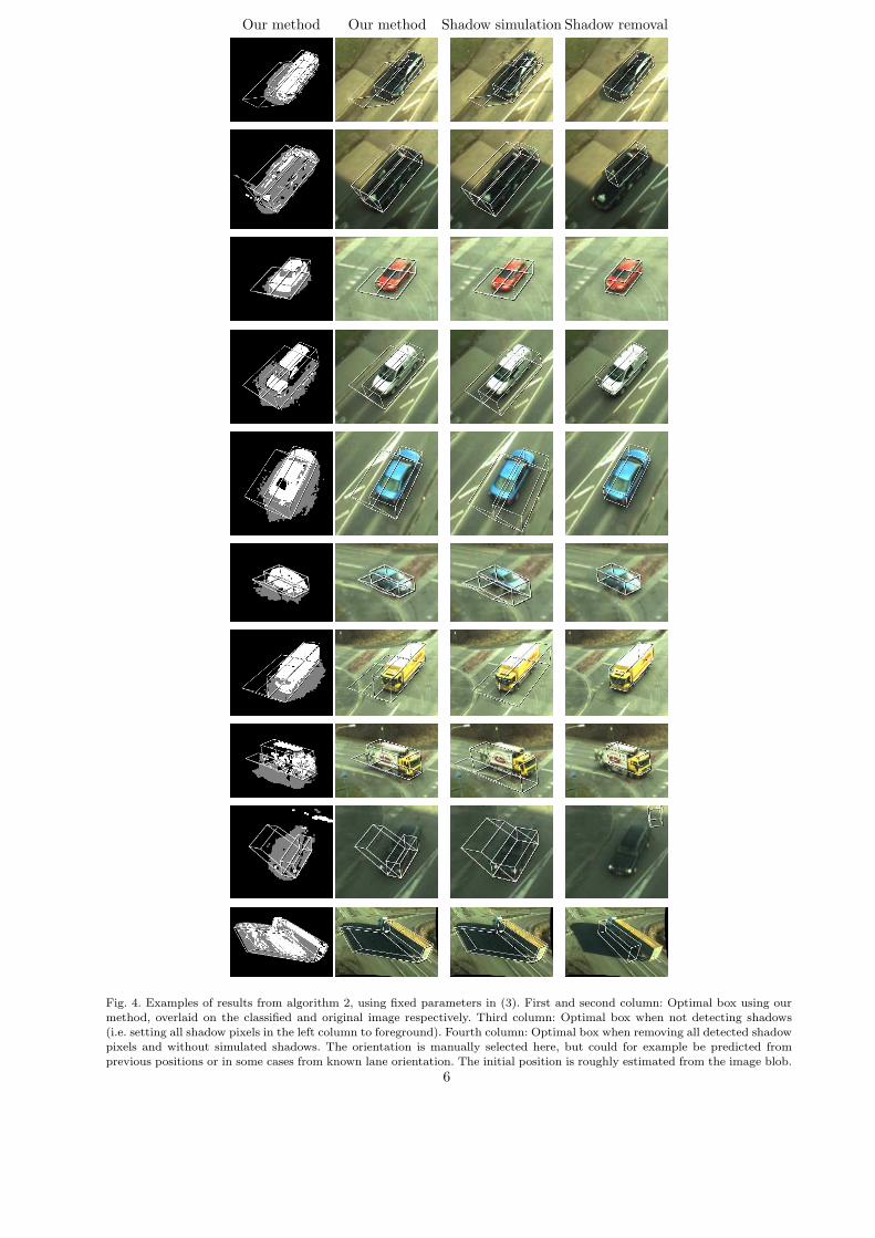
Our method Our method Shadow simulation Shadow removal

Fig. 4. Examples of results from algorithm 2, using fixed parameters in (3). First and second column: Optimal box using ourmethod, overlaid on the classified and original image respectively. Third column: Optimal box when not detecting shadows(i.e. setting all shadow pixels in the left column to foreground). Fourth column: Optimal box when removing all detected shadow

pixels and without simulated shadows. The orientation is manually selected here, but could for example be predicted fromprevious positions or in some cases from known lane orientation. The initial position is roughly estimated from the image blob.

6

Shadow removal Shadow simulation Shadow detection & simulation

#1

#2

Fig. 5. Accumulated trajectories for two different runs in the intersection shown in figure 3, top left. Removal of shadowsreduces detections of vehicles that occupy only a small part of the image (see regions at arrows in left column). Simulating

shadows only helps to detect small vehicles, but introduces clutter (see regions at arrows in centre column) e.g. from shadowsof waving flags, and trees. Shadow detection and simulation allows detection of small objects, without increasing the clutter.

ble result.Moreover, we also tried to add change in orienta-

tion to the list of transformations, but it is too un-stable (at least for some object views) to include afree change in orientation in the optimization whenusing only a single camera view. One solution mightbe to add a punishing term for the orientation in thesimilarity measure, i.e.

s′ = s cos(ϕ0 − ϕ)pϕsign(s) (4)

where ϕ0 is the initial estimated orientation. How-ever, the utility of this rule is still unclear.

We have also made experiments with merging ofestimates from up to four cameras with partly over-lapping views of an intersection. Initially we tried tooptimize the 3D box to all views simultaneously, byadding the similarity measures from each camera.However, this requires a very accurate time synchro-

nization between the cameras. Otherwise the opti-mized box usually becomes larger than the actualvehicle since the box tries to cover all camera blobs(since foreground is rewarded more than backgroundis punished). If the cameras are not fully in sync, itthus appears to be better to optimize to each cameraseparately and then merge the resulting 3D boxesby e.g. averaging the state parameters.

The optimization algorithm is very crude and maysometimes end up in a local optimum if the initialposition is too far from the global optimum. It canthen be useful to add a few more random transfor-mations to the list in algorithm 1, or to use moreelaborate optimization schemes. However, the im-provement has not been significant when initializingthe optimization using a prediction from previousframes (e.g. using a Kalman filter), and the estima-tion of size can also be improved by averaging esti-

7

Algorithm 1 Optimization of box position (fixedsize and orientation). Basically, the algorithm triesdifferent positions, with decreasing step size, aroundthe currently best value/state until the similaritymeasure is no longer increasing.

Let {Tn} = { Increase x, Decrease x, Increase y,Decrease y }, with initially 1 meter step size (thendivided by two a few times during the iterations).

# Given size, orientation, and initial position(L,W,H, x0, y0, ϕ) = ...# Initial optimumsopt = −∞Bopt = {L,W,H, x0, y0, ϕ}# Loop over transformation scalesfor m ∈ [0, ...,M ] do

# Loop over list of transformations as long asoptimum is increasingiter = 0n = 0while iter < |{Tk}| do

iter = iter + 1n = mod(n + 1, |{Tk}|) # Get next transfor-mationBnew = transform(Bopt, Tn/2m) # Trans-form boxSnew = simulate box image(Bnew) # Simu-late a box imagesnew = s(I, Snew) # Compute similarity# Store new optimum if new box is betterif snew > sopt then

sopt = snew

Bopt = Bnew

iter = 0end if

end while

end for

mates in time (as described below).

6. Experiments in a tracking system

We have also used the 3D box optimization in avehicle tracking system. It is beyond the scope of thispaper to describe a fully functional tracking systemfor all traffic situations and weather conditions, butwe will discuss some details and observations here.In essence, the 3D box position estimates are used asmeasurements to an extended Kalman filter (EKF)in the 3D ground plane domain, see figure 6 for anoverview. The details can be worked out in many

Algorithm 2 Optimization of box position and size(fixed orientation). Basically, the algorithm tries dif-ferent sizes in algorithm 1.

# Given orientation, and initial position(x0, y0, ϕ) = ...# Loop over list of box sizessopt = −∞for all (Lk,Wk,HK) in {(Lk,Wk,Hk)} do

# Optimize position using algorithm 1(sk,Bk) = algorithm 1(Lk,Wk,Hk, x0, y0, ϕ)# Store new optimum if new box is betterif sk > sopt then

sopt = sk

Bopt = Bk

end if

end for

Get next frame and dosubtraction/classification

��Predict box state for current

boxes, using Kalman andprevious trajectories

��Estimate/refine 3D box states

using alg. 1-2 if fully visible andonly alg. 1 otherwise

��– Update Kalman filter using 3D box

estimates when considered valid– Update size estimate

��Initiate new boxes and Kalman filters

for segmented regions that are notyet covered by current boxes

BC

EDoo

Fig. 6. Sketch overview of the vehicle tracking system.

different ways, we propose some solutions here.The vehicle size is estimated by weighting to-

gether the estimates from each frame in time. Eachestimate of the (Length,Width,Height) triplet isweighted depending on the view from which the ve-hicle was seen. For example, if the vehicle is viewedfrom above, the height estimate gets a low weightand the length and width get higher weights.

When a vehicle becomes partly occluded (as canbe detected by analyzing the Kalman predictions ofall other current boxes, and manually labeled build-ing regions etc.), it has seemed more stable to lock

8

the size to the current time average estimate dur-ing optimization. Hence, we use algorithm 2 if thebox is considered to be fully visible, and algorithm1 otherwise with other objects marked as invalidpixels in V. Moreover, in cases where shadows arelargely misclassified as foreground, it has appearedto be more robust to also include the regions thatfall within simulated shadows as invalid pixels. Thismeans that the tracker will treat vehicles that fallwithin (simulated) shadows from other vehicles asoccluded.

We use a simple bicycle model in the extendedKalman filter that contains position, orientation,and speed, (x, y, ϕ, v). We basically only get posi-tion measurements, and more complex models maytherefore cause instability. More complex modelscan however be applied as a post-processing step tofurther refine the trajectories.

The box orientation is predicted from the trajec-tory of previously collected estimates, by computingthe tangent at the end of the trajectory in a cer-tain spatial window (initially using the lane orien-tation). It has seemed more stable to use a spatiallybased window rather than a time based window likethe orientation in the Kalman model. For vehiclesthat are temporarily stationary over extended pe-riods the latter estimate may become unstable. Ina recent paper (Atev et al., 2008) (which is an im-proved version of (Atev et al., 2005)), propose an-other model including curvature of the motion pathwhich reduces the stop-and-go problem. But even ifwe use an exact vehicle model, noisy position mea-surements can still in theory make the car appearto move forward and backward and eventually turnaround. It may also be possible to use optical flow asa hint for the orientation, as in e.g. (Song and Neva-tia, 2007), but this only works for moving vehicles.

The 3D box estimates are sometimes corruptedand should then be treated as outliers. Various out-lier tests can be applied such as thresholds for max-imally allowed occlusion (both in 2D and 3D), lowerlimits for pixel area, threshold for maximal fore-ground sparsity inside a box, maximally allowed dis-tance from the prediction, and so on. These testsmay depend on the situation. For example, we havecollected data from an intersection where flag poleson the side of the road cast moving shadows onto theroad, which sometimes initiate new boxes. A 3D testfor overlapping boxes would not allow these boxesto be ‘run over’ by true boxes.

Deciding when to initiate new boxes is also a diffi-cult problem, especially in heavy traffic. In our sys-

tem, new boxes are currently only allowed to be ini-tiated if the segment does not overlap much withexisting boxes. This means that new vehicles mustbe almost fully visible to be initiated, which alsomeans that occluded vehicles that are lost (decidedto be terminated) may disturb neighboring measure-ments.

7. Conclusions

We have in this paper presented an algorithm forestimation of size and position of vehicles that com-bines both shadow detection and shadow simulation.It is shown in some examples and experiments thatthis combination can improve the performance com-pared to only using shadow detection or shadow sim-ulation. The improvement is most evident in caseswhere the shadow detection or the shadow simu-lation is inaccurate. There are some cases thoughwhere one of the comparison methods is somewhatbetter than our method, and a topic for future re-search may be to improve the similarity measureeven further.

The paper also describes an example how to usethe 3D box optimization in a tracking system. How-ever, better performance is still needed in situationswith large occlusions and heavy traffic. This is a wellknown and currently unsolved tracking problem.

Acknowledgment

This work has been supported by the SwedishRoad Administration (SRA) within the IVSSproject Intersection accidents: analysis and preven-

tion.

References

Hakan Ardo, Use of learning for detection and track-ing of vehicles, Proceedings of the Swedish Sym-posium on Image Analysis, 2004

Hakan Ardo and Rikard Berthilsson, AdaptiveBackground Estimation using Intensity Indepen-dent Features, Proceedings of the 2006 BritishMachine and Vision Conference BMVC’06,III:1069, September 2006

Stefan Atev, Nikolaos Papanikolopoulos, Multi-view3D Vehicle Tracking with a Constrained Filter,IEEE International Conference on Robotics andAutomation, 2277–2282, May 2008, Pasadena,CA, USA,

9

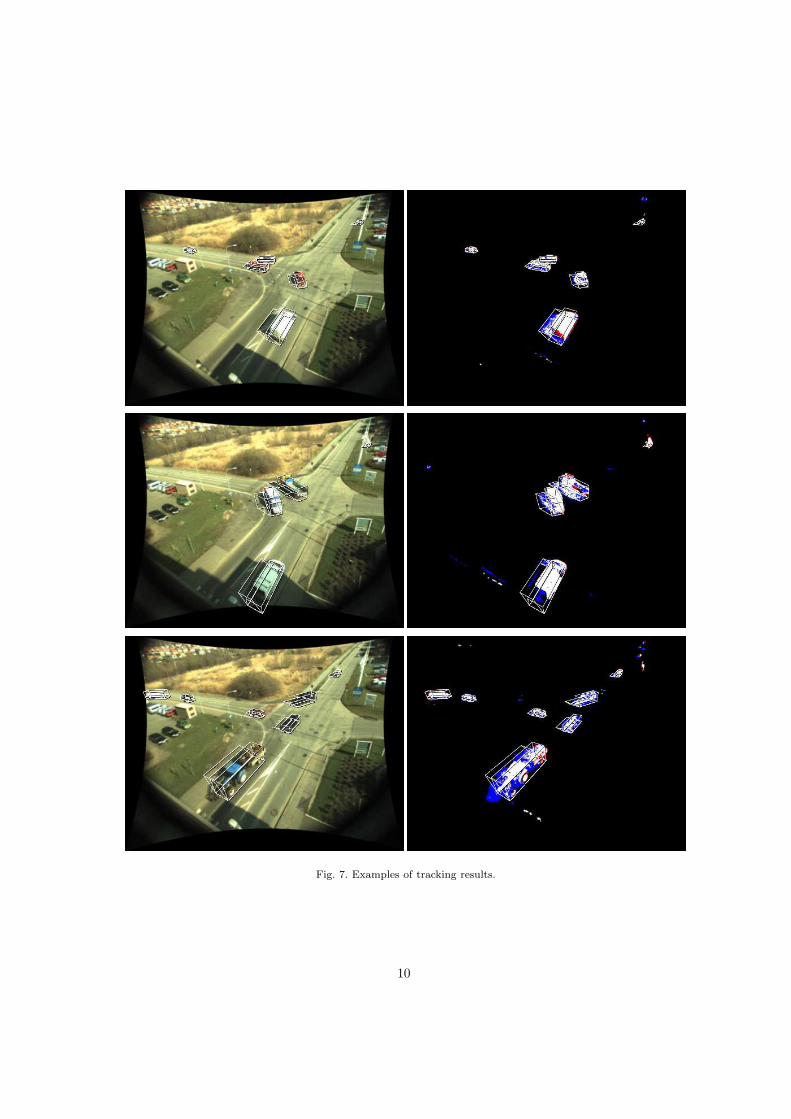
Fig. 7. Examples of tracking results.

10

Stefan Atev, Hemanth Arumugam, Osama Masoud,Ravi Janardan, Nikolaos Papanikolopoulos, AVision-Based Approach to Collision Prediction atTraffic Intersections, IEEE Transactions on Intel-ligent Transportation Systems, 6(4):416–423, De-cember 2005

Christopher M. Bishop, Neural Networks for Pat-tern Recognition, Oxford University Press, 1995,ISBN 0-19-853864-2

Andreas Bockert, Vehicle Detection and Classifica-tion in Video Sequences, Linkoping University,SE-581 83 Linkoping, Sweden, 2002, Masters the-sis LiTH-ISY-EX-3270

Enrique J. Carmona, Javier Martınez-Cantos, JoseMira, A new video segmentation method of mov-ing objects based on blob-level knowledge, Pat-tern Recognition Letters, 29:272-285, 2008

David Claus, Andrew W. Fitzgibbon, A RationalFunction Lens Distortion Model for General Cam-eras, CVPR’05, 2005

Hendrik Dahlkamp, Hans-Hellmut Nagel, ArturOttlik, Paul Reuter, International Journal ofComputer Vision, A Framework for Model-Based Tracking Experiments in Image Sequences,73(2):139–157, 2007

Hendrik Dahlkamp, Arthur E.C. Pece, Artur Ott-lik, Hans-Hellmut Nagel, Differential Analysis ofTwo Model-Based Vehicle Tracking Approaches,DAGM’04, 71–78, 2004

R. Hartley, A. Zisserman, Multiple View Geometryin Computer Vision, Cambridge University Press,2000

Horprasert, T., Harwood, D., Davis, L.S., A Sta-tistical Approach for Real-Time Robust Back-ground Subtraction and Shadow Detection, Pro-ceedings of IEEE ICCV’99 FRAME-RATE Work-shop, 1999

Bjorn Johansson, Johan Wiklund, Gosta Granlund,Goals and status within the IVSS project,Seminar on ”Cognitive vision in trafficanalysis”, May 2006, Lund, Sweden URL:http://www.lth.se/index.php?id=10904

Ajay J. Joshi, Stefan Atev, Osama Masoud, Niko-laos Papanikolopoulos, Moving Shadow Detectionwith Low- and Mid-Level Reasoning, IEEE In-ternational Conference on Robotics and Automa-tion, April 2007

Zu Whan Kim, Jitendra Malik, Fast Vehicle Detec-tion with Probabilistic Feature Grouping and itsApplication to Vehicle Tracking, Proceedings ofICCV’03, 524–531, 2003

Jianguang Lou, Tieniu Tan, Weiming Hu, Hao Yang,

Steven J. Maybank, 3-D Model-Based VehicleTracking, IEEE Transactions on image process-ing, 14(10):1561–1569, October 2005

Derek R. Magee, Tracking multiple vehicles usingforeground, background and motion models, Im-age and Vision Computing, 22:143–155, 2004

Hans-Helmut Nagel, Steps Towards a Cognitive Vi-sion System, AI Magazine, 25(2):31–50, 2004

Andrea Prati, Ivana Mikic, Mohan M. Triveldi,Rita Cucchiara, Detecting Moving Shadows: Al-gorithms and Evaluation, IEEE Transactionson Pattern Analysis and Machine Intelligence,25(7):918–923, 2003

NREL, SOLPOS 2.0. Distributed by the Na-tional Renewable Energy Laboratory. Centerfor Renewable Energy Resources. RenewableResource Data Center, February, 2000, URL:http://rredc.nrel.gov/solar/codes algs/solpos

Xuefeng Song, Ram Nevatia, Detection and Track-ing of Moving Vehicles in Crowded Scenes, IEEEWorkshop on Motion and Video Computing,WMVC’07, 4–4, 2007

C. Stauffer, W. Grimson, Adaptive BackgroundMixture Models for Real-Time Tracking, IEEEConference on Computer Vision and PatternRecognition, 246–252, 1999

John Wood, Statistical Background Models withShadow Detection for Video Based Tracking,Linkoping University, SE-581 83 Linkoping, Swe-den, March, 2007, LiTH-ISY-EX–07/3921–SE

11