link.springer.com SolutionPropertiesofa3DStochasticEulerFluidEquation Dan Crisan1 ·Franco...

Journal of Nonlinear Science (2019) 29:813–870https://doi.org/10.1007/s00332-018-9506-6

Solution Properties of a 3D Stochastic Euler Fluid Equation

Dan Crisan1 · Franco Flandoli2 · Darryl D. Holm1

Received: 17 March 2018 / Accepted: 10 October 2018 / Published online: 20 October 2018© The Author(s) 2018

AbstractWe prove local well-posedness in regular spaces and a Beale–Kato–Majda blow-up criterion for a recently derived stochastic model of the 3D Euler fluid equationfor incompressible flow. This model describes incompressible fluid motions whoseLagrangian particle paths follow a stochastic process with cylindrical noise and alsosatisfy Newton’s second law in every Lagrangian domain.

Keywords Analytical properties · Stochastic fluid equations · Lie derivative estimates

Mathematics Subject Classification 60H15 · 37J15 · 60H30

1 Introduction

The present paper shows that two important analytical properties of deterministicEuler fluid dynamics in three dimensions possess close counterparts in the stochasticEuler fluid model introduced in Holm (2015). The first of these analytical propertiesis the local-in-time existence and uniqueness of deterministic Euler fluid flows. Thesecond property is a criterion for blow-up in finite time due to Beale et al. (1984).For a historical review of these two fundamental analytical properties for determin-istic Euler fluid dynamics, see e.g. Gibbon (2008). We believe this fidelity of thestochastic model of Holm (2015) investigated here with the analytical properties ofthe deterministic case bodes well for the potential use of this model in, for example,uncertainty quantification of either observed or numerically simulated fluid flows. Theneed and inspiration for such a model can be illustrated, for example, by examiningdata from satellite observations collected in the National Oceanic and Atmospheric

Communicated by Paul Newton.

B Darryl D. [email protected]

1 Department of Mathematics, Imperial College, London SW7 2AZ, UK

2 Department of Applied Mathematics, University of Pisa, Via Bonanno 25B, 56126 Pisa, Italy

123

http://crossmark.crossref.org/dialog/?doi=10.1007/s00332-018-9506-6&domain=pdf

http://orcid.org/0000-0001-6362-9912

814 Journal of Nonlinear Science (2019) 29:813–870

Fig. 1 This figure shows latitude and longitude of Lagrangian trajectories of drifters on the ocean surfacedriven by the wind and ocean currents, as compiled from satellite observations by the National Oceanic andAtmospheric Administration Global Drifter Program. Each colour corresponds to a different drifter (seeLilly (2017)). Upon looking carefully at the individual Lagrangian paths in this figure, one sees that eachof them evolves as a mean drift flow, composed with an erratic flow comprising rapid fluctuations aroundthe mean (Colour figure online)

Administration (NOAA) “Global Drifter Program”, a compilation of which is shownin Fig. 1.

Figure 1 (courtesy of Lilly 2017) displays the global array of surface drifter dis-placement trajectories from the National Oceanic and Atmospheric Administration’s“Global Drifter Program” (www.aoml.noaa.gov/phod/dac). In total, more than 10,000drifters have been deployed since 1979, representing nearly 30 million data points ofpositions along the Lagrangian paths of the drifters at 6-h intervals. This large spa-tiotemporal data set is a major source of information regarding ocean circulation,which in turn is an important component of the global climate system. For a recentdiscussion, see for example Sykulski et al. (2016). This data set of spatiotemporalobservations from satellites of the spatial paths of objects drifting near the surfaceof the ocean provides inspiration for further development of data-driven stochasticmodels of fluid dynamics of the type discussed in the present paper.

Inspired by this drifter data, the present paper investigates the existence, uniquenessand singularity properties of a recently derived stochastic model of the Euler fluidequations for incompressible flow (Holm 2015) that is consistent with this data. Forthis purpose, we combine methods from geometric mechanics, functional analysis andstochastic analysis. In the model under investigation, one assumes that the Lagrangianparticle paths in the fluid motion xt = ηt (X) with initial position X ∈ R

3 each followa Stratonovich stochastic process given by

dηt (X) = u(ηt (X), t)dt +∑

i

ξi (ηt (X)) ◦ dBit . (1.1)

123

www.aoml.noaa.gov/phod/dac

Journal of Nonlinear Science (2019) 29:813–870 815

This approach immediately introduces the issue of spatial correlations.In particular, an important feature of the data in Fig. 1 is that the ocean currents

show up as persistent spatial correlations, easily recognized visually as spatial regionsin which the colours representing individual paths tend to concentrate. To capture thisfeature, we transform Lagrangian trajectory description (1.1) into the spatial represen-tation of the Eulerian transport velocity given by the Stratonovich stochastic vectorfield,

dyt (x) = u(x, t)dt +∑

i

ξi (x) ◦ dBit = dηt η

−1t (x) . (1.2)

In Eqs. (1.1) and (1.2), the Bit with i ∈ N are scalar independent Brownian motions,

and the ξi (x) represent the spatial correlations which may be obtained as eigenvectorsof the two-point velocity-velocity correlation matrix Ci j (x, y), i, j = 1, 2, . . . , N , asan integral operator. Namely,

∑

j

∫Ci j (x, y)ξ j (y)dy = λξi (x) . (1.3)

These correlation eigenvectors exhibit a spectrumof spatial scales for the trajectories ofthe drifters, indicating the variety of spatiotemporal scales in the evolution of the oceancurrents which transport the drifters. This feature of the data is worthy of further study.In what follows, we will assume that the velocity correlation eigenvectors ξi (x) withi = 1, . . . , N have been determined by reliable data assimilation procedures, so wemay take them to be prescribed, divergence-free, three-dimensional vector functions.For explicit examples of the process of determining the ξi (x) eigenvectors at coarseresolution from finely resolved numerical simulations, see Cotter et al. (2018a, b).For an extension of this method to include non-stationary correlation statistics, seeGay-Balmaz and Holm (2018).

A rigorous analysis of the stochastic process ηt in (1.1) is under way by the authors.Following from classical results (e.g. Kunita 1984, 1990), we show in a forthcomingpaper that ηt is a temporally stochastic curve on themanifold of smooth invertiblemapswith smooth inverses (i.e. diffeomorphisms). Thus, although the time dependence of ηtin (1.1) is not differentiable, its spatial dependence is smooth. The stochastic processdηt (X) in (1.1) is also the pullback by the diffeomorphism ηt of the stochastic vectorfield dyt (x) in (1.2). That is, η∗

t dyt (x) = dηt (X) (see e.g. Holm (2015) for details).Conversely, the stochastic vector field in (1.2) is the Eulerian representation in fixedspatial coordinates x of the stochastic process in (1.1) for the Lagrangian fluid parcelpaths, labelled by their Lagrangian coordinates X .

The expression for the Lagrangian trajectories in Eq. (1.1) is clearly in accordwith the observed behaviour of the Lagrangian trajectories displayed in Fig. 1. More-over, expression (1.2) for the corresponding Eulerian transport velocity has beenderived recently in Cotter et al. (2017) by using multi-time homogenization meth-ods for Lagrangian trajectories corresponding to solutions of the deterministic Eulerequations, in the asymptotic limit of timescale separation between the mean and fluc-tuating flow. In particular, the fluctuating dynamics in the second term in (1.2) has been

123


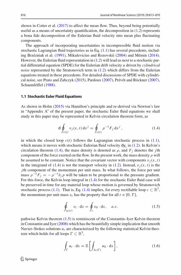
shown in Cotter et al. (2017) to affect the mean flow. Thus, beyond being potentiallyuseful as a means of uncertainty quantification, the decomposition in (1.2) representsa bona fide decomposition of the Eulerian fluid velocity into mean plus fluctuatingcomponents.

The approach of incorporating uncertainties in incompressible fluid motion viastochastic Lagrangian fluid trajectories as in Eq. (1.1) has several precedents, includ-ing Brzézniak et al. (1991), Mikulevicius and Rozovskii (2004) and Mémin (2014).However, the Eulerian fluid representation in (1.2) will lead us next to a stochastic par-tial differential equation (SPDE) for the Eulerian drift velocity u driven by cylindricalnoise represented by the Stratonovich term in (1.2) which differs from the Eulerianequations treated in these precedents. For detailed discussions of SPDE with cylindri-cal noise, see Prato and Zabczyk (2015), Pardoux (2007), Prévôt and Röckner (2007),Schaumlöffel (1988).

1.1 Stochastic Euler Fluid Equations

As shown in Holm (2015) via Hamilton’s principle and re-derived via Newton’s lawin “Appendix A” of the present paper, the stochastic Euler fluid equations we shallstudy in this paper may be represented in Kelvin circulation theorem form, as

d∮

c(t)v j (x, t) dx

j =∮

c(t)ρ−1Fj dx

j , (1.4)

in which the closed loop c(t) follows the Lagrangian stochastic process in (1.1),which means it moves with stochastic Eulerian fluid velocity dyt in (1.2). In Kelvin’scirculation theorem (1.4), the mass density is denoted as ρ, and Fj denotes the j thcomponent of the force exerted on the flow. In the present work, themass density ρ willbe assumed to be constant. Notice that the covariant vector with components v j (x, t)in the integrand of (1.4) is not the transport velocity in (1.2). Instead, v j (x, t) is thej th component of the momentum per unit mass. In what follows, the force per unitmass ρ−1Fj = − ρ−1∂ j p will be taken to be proportional to the pressure gradient.For this force, the Kelvin loop integral in (1.4) for the stochastic Euler fluid case willbe preserved in time for any material loop whose motion is governed by Stratonovichstochastic process (1.1). That is, Eq. (1.4) implies, for every rectifiable loop c ⊂ R

3,the momentum per unit mass vt has the property that for all t ∈ [0, T ],

∮

ηt (c)vt · dx =

∮

cv0 · dx, a.s. (1.5)

pathwise Kelvin theorem (1.5) is reminiscent of the Constantin–Iyer Kelvin theoreminConstantin and Iyer (2008) which has the beautifully simple implication that smoothNavier–Stokes solutions ut are characterized by the following statistical Kelvin theo-rem which holds for all loops � ⊂ R

3,

∫

�

ut · dx = E

[∫

At (�)

u0 · dx]

, (1.6)

123


where At is the back-to-labels map for a stochastic flow of a certain forward Itôequation and E denotes expectation for that flow. Unlike pathwise Kelvin theorem(1.5) which holds for solutions of the stochastic Euler fluid equations, Constantin–Iyer Kelvin theorem in (1.6) is completely deterministic, since the fluid velocity ut isa solution of the Navier–Stokes equations. For more discussion of Kelvin circulationtheorems for stochastic Euler fluid equations, see Drivas and Holm (2018).

In the case of the stochastic Euler fluid treated here in Euclidean coordinates,applying the Stokes theorem to the Kelvin loop integral in (1.4) yields the equationfor ω = curl v proposed in Holm (2015), as

dω + (dyt · ∇)ω − (ω · ∇)dyt = 0 , ω|t=0 = ω0 , (1.7)

where the loop integral on the right-hand side of (1.4) vanishes for pressure forceswith constant mass density.

Main Results This paper shows that two well-known analytical properties of the deter-ministic 3D Euler fluid equations are preserved under the stochastic modification in(1.7) we study here. First, 3D stochastic Euler fluid vorticity Eq. (1.7) is locally well-posed in the sense that it possesses local-in-time existence and uniqueness of solutions,for initial vorticity in the spaceW 2,2(R3) (Ebin and Marsden 1970). See Lichtenstein(1925) as mentioned in Frisch and Villone (2014) for a historical precedent for localexistence and uniqueness for the Euler fluid equations. Second, vorticity Eq. (1.7) alsopossesses a Beale–Kato–Majda (BKM) criterion for blow-up which is identical to theone proved for the deterministic Euler fluid equations in Beale et al. (1984).

Theorem 1 (Existence and uniqueness) Given initial vorticity ω0 ∈ W 2,2(T3,R3

),

there exists a local solution in W 2,2 of stochastic 3D Euler Eq. (1.7). Namely, ifω(1), ω(2) : × [0, τ ]× T

3 → R3 are two solutions defined up to the same stopping

time τ > 0, then ω(1) = ω(2).

Our result corresponding to the celebrated Beale–Kato–Majda characterization ofblow-up (Beale et al. 1984) is stated in the following.

Theorem 2 (Beale–Kato–Majda criterion for blow-up) Given initial ω0 ∈ W 2,2(T3,R3

), there exists a stopping time τmax : → [0,∞] and a process ω :

× [0, τmax) × T3 → R

3 with the following properties:

(i) (ω is a solution) The process t → ω (t ∧ τmax, ·) has trajectories that are almostsurely in the class C

([0, τmax);W 2,2(T3;R3

))and Eq. (1.7) holds as an identity

in L2(T3;R3

). In addition, τmax is the largest stopping time with this property;

and(ii) (Beale–Kato–Majda criterion Beale et al. 1984) If τmax < ∞, then

∫ τmax

0‖ω (t) ‖∞dt = +∞

and, in particular, lim supt↑τmax‖ω (t)‖∞ = +∞.

123


Plan of the Paper

• Section 2 discusses our assumptions and summarizes the main results of the paper.

– Section 2.1 formulates our objectives and sets the notation.– Section 2.2 discusses the cylindrical noise properties of (1.1) and providesbasic bounds on the Lie derivatives needed in proving the main analyticalresults.

– Section 2.3 provides additional definitions needed in the context of explainingthe main results of the paper.

• Section 3 provides proofs of the main results

– Sections 3.1 and 3.3 prove the uniqueness properties needed for establishingTheorem 1.

– Section 3.5 introduces a cut-off function which is instrumental in the proof ofthe BKM theorem for the stochastic Euler equations given in Section 3.4.

• Section 4 summarizes the proofs of several key technical results which are sum-moned in establishing Theorems 1 and 2.

– Section 4.1 discusses fractional Sobolev regularity in time.– Section 4.2 provides the a priori bounds needed to prove estimate (3.19).– Section 4.3 proves the bounds needed to complete the proof that estimate (3.19)is uniform in time.

– Section 4.4 establishes the key estimates for the bounds involving Lie deriva-tives that are needed in the proofs.

• “Appendix A” provides a new derivation of the stochastic Euler equations intro-duced in Holm (2015) from the viewpoint of Newton’s second law and derivesthe corresponding Kelvin circulation theorem. The deterministic (resp. stochastic)equations of motion are derived using the pullback of Newton’s second law by thedeterministic (resp. stochastic) diffeomorphism describing the Lagrange-to-Eulermap. The Kelvin circulation theorems for both cases are then derived from theircorresponding Newtonian 2nd Laws. The importance of the distinction betweentransport velocity and transported momentum is emphasized in “Appendix A”for both the deterministic and stochastic Newton’s Laws and Kelvin’s circulationtheorems.

2 Assumptions andMain Results

2.1 Formulating Objectives and Setting Notation

Our aim fromnowonwill be to prove local-in-time existence and uniqueness of regularsolutions of the stochastic Euler vorticity equation

dω + Lvωdt +∞∑

k=1

Lξkω ◦ dBkt = 0, ω|t=0 = ω0, (2.1)

123


whichwas proposed inHolm (2015).Here,Lvω (resp.Lξkω) denotes theLie derivativewith respect to the vector fields v (resp. ξk) as in (A.27) applied to the vorticity vectorfield. In particular,

Lξkω = (ξk · ∇)ω − (ω · ∇)ξk = [ ξk , ω ] . (2.2)

A natural question is whether we should sum only over a finite number of termsor, on the contrary, it is important to have an infinite sum, and not only for generality.An important remark is that a finite number of eigenvectors arises in the relevant caseassociated with a “data-driven” model based on what is resolvable in either numericsof observations, and it would simplify some technical issues [we do not have to assume(2.11)]. However, an infinite sum could be of interest in regularization-by-noise inves-tigations: see an example in Delarue et al. (2014) (easier than 3D Euler equations)where a singularity is prevented by an infinite-dimensional noise. However, it is alsotrue that in some cases a finite-dimensional noise is sufficient also for regularizationby noise (see examples in Flandoli et al. (2010, 2011, 2014)).

As mentioned in Remark 32, for the case of the Euler fluid equations treated here inCartesian R

3 coordinates, the two velocities denoted u and v in the previous sectionmay be taken to be identical vectors for the case at hand in R3. Consequently, for theremainder of the present work, in a slight abuse of notation, we simply let v denote theboth fluid velocity and the momentum per unit mass. Then, ω = curl v is the vorticity,and ξk comprise N divergence-free prescribed vector fields, subject to the assumptionsstated below. The processes Bk with k ∈ N are scalar independent Brownian motions.The result we present next will extend the known analogous result for deterministicEuler equations to the stochastic case.

To simplify some of the arguments, we will work on a torusT3 = R3/Z3. However,

the results should also hold in the full space, R3.Stochastic Euler vorticity Eq. (2.1) above is stated in Stratonovich form. The cor-

responding Itô form is

dω + Lvωdt +∞∑

k=1

Lξk ωdBkt = 1

2

∞∑

k=1

L2ξk

ω dt , ω|t=0 = ω0 , (2.3)

where we write

L2ξk

ω = Lξk (Lξkω) = [ξk , [ξk , ω]] ,

for the double Lie bracket of the divergence-free vector field ξk with the vorticityvector field ω. Indeed, let us recall that Stratonovich integral is equal to Itô integralplus one half of the corresponding cross-variation process1:

∫ t

0Lξkωs ◦ dBk

s =∫ t

0LξkωsdB

ks + 1

2

[Lξkω, Bk

]

t.

1 The subscript t on the square brackets distinguishes between the cross-variation process and Lie bracketof vector fields. To avoid confusion between these two uses of the square bracket, we will denote the Liebracket operation [ ξk , · ] by the symbol Lξk ·, as in Eq. (2.2).

123


By the linearity and the space independence of Bk ,[Lξkω, Bk

]t = Lξk

[ω, Bk

]t . Asωt

has the form dωt = atdt+∑h bht ◦dBh

t , where Bh are independent, the cross-variation

process[ω, Bk

]t is given by

[ω, Bk

]

t=∫ t

0bks ds.

In our case bks = −Lξkωs , hence

[ω, Bk

]

t= −

∫ t

0Lξkωsds.

Finally

Lξk

[ω, Bk

]

t= −

∫ t

0L2

ξkωsds

and therefore, in differential form,

Lξkωt ◦ dBkt = Lξkωt dB

kt − 1

2L2

ξkωtdt .

Among different possible strategies to study Eq. (2.3), some of them based onstochastic flows, we present here the extension to the stochastic case of a classicalPDE proof (see, for instance, Kato and Lai 1984; Lions 1996; Majda and Bertozzi2002).

The proof is based onapriori estimates in high-order Sobolev spaces. The determin-istic classical result proves well-posedness in the space ω (t) ∈ W 3/2+ε,2

(T3;R3

),

for some ε > 0, when ω0 belongs to the same space. Here we simplify (dueto a number of new very non-trivial facts outlined in Sect. 4.2) and work in thespace ω (t) ∈ W 2,2

(T3;R3

). Consequently, we may consider �ω (t) (to avoid frac-

tional derivatives) and investigate existence and uniqueness in the class of regularity�ω (t) ∈ L2

(T3;R3

).

If f , g ∈ L2(T3;R3

), we write 〈 f , g〉 = ∫

T3 f (x) · g (x) dx . We consider thebasis of L2

(T3;C) of functions {e2π iξ ·x ; ξ ∈ Z

3}, and for every f ∈ L2

(T3;C),

we introduce the Fourier coefficients f (ξ) = ∫T3 e−2π iξ ·x f (x) dx , ξ ∈ Z

3; Parseval

identity states that∫T3 | f (x)|2 dx = ∑

ξ∈Z3

∣∣ f (ξ)∣∣2. If v ∈ L2

(T3;R3

)is a vector

field with components vi , i = 1, 2, 3, we write v (ξ) = ∫T3 e2π iξ ·xv (x) dx and we

may easily check using the components that have∫T3 |v (x)|2 dx = ∑

ξ∈Z3 |v (ξ)|2.Since functions which are partial derivatives of other functions, on the torus, musthave zero average, we shall always restrict ourselves to functions f ∈ L2

(T3;C)

such that∫T3 f (x) dx = 0. In this case, f (0) = 0 and the term with ξ = 0 does not

appear in the sums above.We introduce, for every s ≥ 0, the fractional Sobolev space Ws,2

(T3;C) of all

f ∈ L2(T3;C) such that

123


‖ f ‖2Ws,2 :=∑

ξ∈Z3\{0}|ξ |2s ∣∣ f (ξ)

∣∣2 < ∞.

As stated above,we are assuming zero average functions; hence,we have excluded ξ =0.We denote byWs,2

σ

(T3,R3

)the space of all zero mean divergence-free (divergence

in the sense of distribution) vector fields v ∈ L2(T3;R3

)such that all components

vi , i = 1, 2, 3, belong to Ws,2(T3;C). For a vector field v ∈ Ws,2

σ

(T3,R3

), the

norm ‖v‖Ws,2 is defined by the identity ‖v‖2Ws,2

σ

= ∑3i=1 ‖vi‖2Ws,2 , where ‖vi‖2Ws,2

is defined above. We thus have again ‖v‖2Ws,2

σ

:= ∑ξ∈Z3\{0} |ξ |2s |v (ξ)|2. For

f ∈ Ws,2(T3;C), we denote by (−�)s/2 f the function of L2

(T3;C) with Fourier

coefficients |ξ |s f (ξ). Similarly, we write −�−1 f for the function having Fouriercoefficients |ξ |−2 f (ξ). We use the same notations for vector fields, meaning that theoperations are made componentwise.

TheBiot–Savart operator is the reconstruction of a zeromeandivergence-free vectorfield u from a divergence-free vector field ω such that curl u = ω. On the torus,it is given by u = − curl�−1ω. In Fourier components, it is given by u (ξ) =|ξ |−2 ξ × ω (ξ). We have the following well-known result: for all s ≥ 0

‖u‖Ws+1,2σ

≤ ‖ω‖Ws,2σ

. (2.4)

Indeed, using the definition given above of ‖u‖2Ws+1,2

σ

, the formula which relates u (ξ)

to ω (ξ) and the rule |a × b| ≤ |a| |b|, we get

‖u‖2Ws+1,2

σ=

∑

ξ∈Z3\{0}|ξ |2s+2 |u (ξ)|2 =

∑

ξ∈Z3\{0}|ξ |2s+2 |ξ |−4 |ξ × ω (ξ)|2

≤∑

ξ∈Z3\{0}|ξ |2s+2 |ξ |−2 |ω (ξ)|2

and the latter is precisely equal to ‖ω‖Ws,2σ, by the definition above.

We shall denote the dual operator of the Lie derivative Lα of a vector field as L∗α ,

defined by the identity

⟨L∗αβ, γ

⟩ = 〈β,Lαγ 〉 ,

for all smooth vector fields α, β, γ . When div α = 0, the dual Lie operator is given invector components by

(L∗αγ)i := −

∑

j

(α j∂ jγi + γ j∂iα

j)

. (2.5)

123


2.2 Assumptions on {�k} and Basic Bounds on Lie Derivatives

We assume that the vector fields ξk : T3 → R3 are of class C4 and satisfy

∥∥∥∥∥

∞∑

k=1

L2ξkf

∥∥∥∥∥

2

L2

≤ C ‖ f ‖2W 2,2 (2.6)

∞∑

k=1

⟨Lξk f ,Lξk f⟩ ≤ C ‖ f ‖2W 2,2 (2.7)

for all f ∈ W 2,2(T3;R3

)and

∞∑

k=1

‖ξk‖2W 3,2 < ∞. (2.8)

These properties will be used below, both to give a meaning to the stochastic terms inthe equation and to prove certain bounds. In addition, a recurrent energy-type scheme inour proofs requires comparisons of quadratic variations and Stratonovich corrections.

Making these comparisons leads to sums of the form⟨L2

ξkf , f

⟩+ ⟨Lξk f ,Lξk f

⟩. In

dealing with them, we have observed the validity of two striking bounds, which apriori may look surprising. They are:

⟨L2

ξkf , f

⟩+ ⟨Lξk f ,Lξk f

⟩ ≤ C (0)k ‖ f ‖2L2 (2.9)

⟨�L2

ξkf ,� f

⟩+ ⟨

�Lξk f ,�Lξk f⟩ ≤ C (2)

k ‖ f ‖2W 2,2 , (2.10)

for suitable constants C (0)k ,C (2)

k . For these estimates to hold, the regularity of f mustbe, respectively, W 2,2

(T3;R3

)and W 4,2

(T3;R3

). The proofs of estimates (2.9) and

(2.10) are given in Sect. 4.4.2

Concerning inequality (2.9), it is clear that the second-order terms in⟨L2

ξkf , f

⟩and

⟨Lξk f ,Lξk f⟩will cancel. However, the cancellations among the first-order terms are

not so obvious. Remarkably, though, these terms do cancel each other, so that only thezero-order terms remain. Similar remarks apply to the other inequality.

In addition, we must assume

∞∑

k=1

C (0)k < ∞,

∞∑

k=1

C (2)k < ∞. (2.11)

Because the constants C (i)k are rather complicated, we will not write them explicitly

here. In the relevant case of a finite number of ξk’s, there is obviously no need of this

2 We thank Istvan Gyöngy and Nikolai Krylov for pointing out to us that estimates such as (2.9) and (2.10)hold in much more generality (see e.g. Gyöngy (1989), Gyöngy and Krylov (1992), Gyöngy and Krylov(2003)).

123


assumption. In the case of infinitely many terms, see a sufficient condition in Remark28 of Sect. 4.4.

2.3 Statement of theMain Results

Let{Bk}k∈N be a sequence of independent Brownian motions on a filtered probability

space (,F ,Ft , P). We do not use the most common notation � for the probabilityspace, since ω is the traditional notation for the vorticity. Thus, the elementary eventswill be denoted by θ ∈ . Let {ξk}k∈N be a sequence of vector fields, satisfying theassumptions of Sect. 2.2. Consider Eq. (2.3) on [0,∞).

Definition 3 (Local solution) A local solution in W 2,2σ of the stochastic 3D Euler

Eq. (2.3 ) is given by a pair (τ, ω) consisting of a stopping time τ : → [0,∞)

and a process ω : × [0, τ ] × T3 → R

3 such that a.e. the trajectory is of classC([0, τ ] ;W 2,2

σ

(T3;R3

)), ω (t ∧ τ, ·), is adapted to (Ft ), and Eq. (2.3) holds in the

usual integral sense; more precisely, for any bounded stopping time τ ≤ τ

ωτ − ω0 +∫ τ

0Lvωdt +

∞∑

k=1

∫ τ

0LξkωdB

kt = 1

2

∞∑

k=1

∫ τ

0L2

ξkω dt (2.12)

holds as an identity in L2(T3;R3

).

Definition 4 (Maximal solution) A maximal solution of (2.3) is given by a stoppingtime τmax : → [0,∞] and a process ω : × [0, τmax) × T

3 → R3 such that: (i)

P (τmax > 0) = 1, τmax = limn→∞ τn where τn is an increasing sequence of stoppingtimes, and (ii) (τn, ω) is a local solution for every n ∈ N; In addition, τmax is thelargest stopping time with properties (i) and (ii). In other words, if (τ ′, ω′) is anotherpair that satisfies (i) and (ii) and ω′ = ω on [0, τ ′ ∧ τmax), then, τ ′ ≤ τmax P-almostsurely.

Remark 5 Due to assumptions (2.6) and (2.7) and the regularity of ω, the two termsrelated to the noise in Eq. (2.3) are well defined, as elements of L2

(T3;R3

).

Remark 6 Recall that, for every α ≥ 0, ω (t) ∈ Wα,2(T3;R3

)implies v (t) ∈

Wα+1,2(T3;R3

). Hence, solutions in W 2,2 have paths such that v ∈ C

([0, τ ] ;W 3,2

(T3;R3

)). Moreover, recall that Wα,2

(T3;R3

) ⊂ C(T3;R3

)for α > 3/2. There-

fore, ω ·∇v ∈ C([0, τ ] × T

3;R3)and v ·∇ω is at least in C

([0, τ ] ;W 1,2

(T3;R3

)),

hence at least

[v, ω] ∈ C([0, τ ] ;W 1,2

(T3;R3

))a.s.

which explainswhy the term [v, ω] is in L2(T3;R3

). (Recall thatDefinition 3 instructs

us to interpret Eq. (2.3) as an identity in L2(T3;R3

).)

123


Remark 7 If ω : × [0, τ ] × T3 → R

3 has the regularity properties of Definition 3and satisfies Eq. (2.3) only in a weak sense, namely, for any bounded stopping timeτ ≤ τ

〈ω (τ ) , φ〉 +∫ τ

0

⟨ω (s) ,L∗

v(s)φ⟩ds +

∞∑

k=1

∫ τ

0

⟨ω (s) ,L∗

ξkφ⟩Bks

= 〈ω0, φ〉 + 1

2

∞∑

k=1

∫ τ

0

⟨ω (s) ,L∗

ξkL∗

ξkφ⟩ds

for all φ ∈ C∞ (T3;R3

), then, by integration by parts, it satisfies Eq. (2.3) as an

identity in L2(T3;R3

).

Theorem 8 Given ω0 ∈ W 2,2σ

(T3,R3

), there exists a maximal solution (τmax, ω) of

the stochastic 3D Euler Eq. (2.3). Moreover, if(τ ′, ω′) is another maximal solution of

(2.3), then necessarily τmax = τ ′ and ω = ω′on [0, τmax). Moreover, either τmax = ∞or lim supt↑τmax

‖ω (t)‖W 2,2 = +∞.

In this paper, we will also prove a corresponding result to the celebrated Beale–Kato–Majda criterion for blow-up of vorticity solutions of the deterministic Euler fluidequations.


(T3,R3

), if τmax < ∞, then

∫ τmax

0‖ω (t)‖∞ dt = +∞ .

In particular, lim supt↑τmax‖ω (t)‖∞ = +∞ almost surely.

Remark 10 As in the deterministic case, Theorem 9 can be used as a criterion for test-ing whether a given numerical simulation has shown finite-time blow-up. FollowingGibbon (2008), the classical Beale–Kato–Majda theorem implies that algebraic singu-larities of the type ‖ω‖∞ ≥ (t∗ − t)−p must have p ≥ 1. In our paper, we have shownthat a corresponding BKM result also applies for the stochastic Euler fluid equations;hence, the same criterion applies here. In Constantin et al. (1996), the L∞ condition inthe BKM theorem was reduced to L p, for finite p, at the price of imposing constraintson the direction of vorticity. We hope to obtain a similar L∞ result for the stochastic3D-Euler equation in future work.

In Sects. 3.1 and 3.2, we prove uniqueness. The rest of the paper will be devotedto proving local existence of the solution and Theorem 9.

123


3 Proofs of theMain Results

3.1 Local Uniqueness of the Solution of the Stochastic 3D Euler Equation

In the following proposition, we prove that any two local solutions of the stochastic3D Euler Eq. (2.3) that are defined up to the same stopping time must coincide. Theproof hinges on bound (2.9) and assumption (2.11).

Proposition 11 Let τ be a stopping time and ω(1), ω(2) : [0, τ ) × T3 → R

3 be twosolutions with paths of class C

([0, τ );W 2,2σ

(T3;R3

))that satisfy the stochastic 3D

Euler Eq. (2.3). Then ω(1) = ω(2) on [0, τ ).

Proof We have that3

dω(i) + Lv(i)ω(i) dt +

∞∑

k=1

Lξkω(i) dBk

t = 1

2

∞∑

k=1

L2ξk

ω(i) dt, i = 1, 2,

where ω(i) = curl v(i). The difference � = ω(1) − ω(2) satisfies

d� + Lv(1)ω(1) dt − Lv(2)ω

(2) dt +∞∑

k=1

Lξk� dBkt = 1

2

∞∑

k=1

L2ξk

� dt

and thus (set also V = v(1) − v(2))

d� + LVω(1) dt + Lv(2)� dt +∞∑

k=1

Lξk� dBkt = 1

2

∞∑

k=1

L2ξk

� dt .

It follows

1

2d ‖�‖2L2 +

⟨LVω(1), �

⟩dt + ⟨Lv(2)�,�

⟩dt +

∞∑

k=1

⟨Lξk�,�⟩dBk

t

= 1

2

∞∑

k=1

⟨L2

ξk�,�

⟩dt + 1

2

∞∑

k=1

⟨Lξk�,Lξk�⟩dt .

We rewrite

⟨LVω(1), �

⟩+ ⟨Lv(2)�,�

⟩

=⟨V · ∇ω(1), �

⟩−⟨ω(1) · ∇V ,�

⟩+⟨v(2) · ∇�,�

⟩−⟨� · ∇v(2), �

⟩

3 The following identity and all the subsequent ones hold as identities in L2(T3;R3

)and represent the

differential form of their integral version in the same way as Eq. (2.3) is the differential form of (2.12).

123


and use the following inequalities:

∣∣∣⟨V · ∇ω(1), �

⟩∣∣∣ ≤ ‖�‖L2 ‖V ‖L4

∥∥∥∇ω(1)∥∥∥L4

≤ C∥∥∥ω(1)

∥∥∥W 2,2

‖�‖2L2

∣∣∣⟨ω(1) · ∇V ,�

⟩∣∣∣ ≤ ‖�‖L2 ‖∇V ‖L2

∥∥∥ω(1)∥∥∥L∞ ≤ C

∥∥∥ω(1)∥∥∥W 2,2

‖�‖2L2

⟨v(2) · ∇�,�

⟩= 0

∣∣∣⟨� · ∇v(2), �

⟩∣∣∣≤‖�‖2L2

∥∥∥∇v(2)∥∥∥L∞ ≤‖�‖2L2

∥∥∥∇v(2)∥∥∥W 2,2

≤C∥∥∥ω(2)

∥∥∥W 2,2

‖�‖2L2 .

Here and below, we repeatedly use the Sobolev embedding theorems

W 2,2(T3)

⊂ Cb

(T3)

, W 2,2(T3)

⊂ W 1,4(T3)

(3.1)

and the fact that Biot–Savart map ω → v maps Wα,p into Wα+1,p for all α ≥ 0 andp ∈ (1,∞). Ws,2

σ into Ws+1,2σ for all s ≥ 0; see (2.4). For instance, the sequences of

inequalities used above in the case of the terms ‖V ‖L4 and∥∥∇v(2)

∥∥L∞ were

‖V ‖L4 ≤ C ‖V ‖W 1,2 ≤ C ′ ‖�‖L2∥∥∥∇v(2)∥∥∥L∞ ≤ C

∥∥∥∇v(2)∥∥∥W 2,2

≤ C ′∥∥∥v(2)

∥∥∥W 3,2

≤ C ′′∥∥∥ω(2)

∥∥∥W 2,2

.

We omit similar detailed explanations sometimes below, when they are of the samekind.

Using also (2.11), we get

d ‖�‖2L2 + 2∞∑

k=1


t ≤ C(1 +

∥∥∥ω(1)∥∥∥W 2,2

+∥∥∥ω(2)

∥∥∥W 2,2

)‖�‖2L2 dt .

Then

d(eY ‖�‖2L2

)= − eY ‖�‖2L2 C

(1 +

∥∥∥ω(1)∥∥∥W 2,2

+∥∥∥ω(2)

∥∥∥W 2,2

)+ eY d ‖�‖2L2

≤ −2eY∞∑

k=1


t ,

where Y is defined as

Yt := −∫ t

0C(1 +

∥∥∥ω(1)s

∥∥∥W 2,2

+∥∥∥ω(2)

s

∥∥∥W 2,2

)ds.

The inequality (recall �0 = 0)

eYτ ‖�τ‖2L2 ≤ −2∞∑

k=1

∫ τ

0eYs

⟨Lξk�s,�s⟩dBk

s

123


holds for every bounded stopping time τ ∈ [0, τ ]. Hence, we have

eYt∧τ ‖�t∧τ‖2L2 ≤ −2∞∑

k=1

∫ t∧τ

0eYs

⟨Lξk�s,�s⟩dBk

s

= − 2∞∑

k=1

∫ t

01s≤τ e

Ys⟨Lξk�s,�s

⟩dBk

s .

In expectation, denoted E, this implies

E

[eYt∧τ ‖�t∧τ‖2L2

]≤ 0

namely E[eYt∧τ ‖�t∧τ‖2L2

] = 0 and thus, for every t ,

eYt∧τ ‖�t∧τ‖2L2 = 0 a.s.

Since Yt∧τ < ∞ a.s., we get ‖�t∧τ‖2L2 = 0 a.s. and thus

ω(1)t∧τ = ω

(2)t∧τ a.s.

Recalling the continuity of trajectories, this implies

ω(1) = ω(2) a.s.

The proof of the proposition is complete. ��

3.2 Existence of a Maximal Solution

Given R > 0, consider the modified Euler equations

dωR + κR (ωR)LvRωR dt +∞∑

k=1

LξkωRdBkt = 1

2

∞∑

k=1

L2ξk

ωR dt, ωR |t=0 = ω0,

(3.2)whereωR = curl vR . In (3.2), κR (ω) := fR(‖∇v‖∞), where fR is a smooth function,equal to 1 on [0, R], equal to 0 on [R + 1,∞) and decreasing in [R, R + 1].

Lemma 12 Given R > 0 and ω0 ∈ W 2,2σ

(T3,R3

), let ωR : × [0,∞) × T

3 → R3

be a global solution in W 2,2 of Eq. (3.2). Let

τR = inf

{t ≥ 0 : ‖ω‖W 2,2 ≥ R

C

},

where C is a constant chosen so that

‖∇v‖∞ ≤ C ‖ω‖W 2,2 .

123


Finally, let ω : × [0, τR] × T3 → R

3 be the restriction of ωR. Then, ω is a localsolution in W 2,2

σ of stochastic 3D Euler Eq. (2.3)

Proof Obviously, because for t ∈ [0, τR] we have ‖∇v‖∞ ≤ C ‖ω‖W 2,2 ≤ R andthus κR (ωR) = 1; namely, the equations are the same. ��

The following proposition is the cornerstone of the existence and uniqueness of amaximal solution of stochastic 3D Euler Eq. (2.3)

Proposition 13 Given R > 0 and ω0 ∈ W 2,2σ

(T3,R3

), there exists a global solution

in W 2,2σ of Eq. (3.2). Moreover, if ω(1)

R , ω(2)R : × [0,∞) ×T

3 → R3 are two global

solutions in W 2,2σ of Eq. (3.2 ), then ω

(1)R = ω

(2)R .

We postpone the proof of Proposition 13 to the later sections. For now, let us showhow it implies the existence of a maximal solution.


(T3,R3

), there exists a maximal solution (τmax, ω) of

stochastic 3DEuler Eq. (2.3). Moreover, either τmax = ∞ or lim supt↑τmax‖ω (t)‖W 2,2

= +∞.

Proof Choose R = n in Lemma 12, then (τn, ωn) is a local solution in W 2,2σ of

stochastic 3D Euler Eq. (2.3). Moreover, define τmax := limn→∞ τn and define ω asω|[0,τn) := ωCn|[0,τn). By uniqueness ωm |[0,τn) := ωn|[0,τn) for any m ≥ n. So ω isconsistently defined.

The statement that either τmax = ∞ or lim supt↑τmax‖ω (t)‖W 2,2 = +∞ is obvious:

if τmax < ∞, then by the continuity of ω on [0, τmax), there exist some random timesτn < τn such that τn − τn ≤ 1

n and that ‖ω (τn)‖W 2,2 ≥ n−1C . Then,

lim supt↑τmax

‖ω (t)‖W 2,2 ≥ lim supn↑∞

‖ω (τn)‖W 2,2 = ∞.

We prove by contradiction that (τmax, ω) is a maximal solution. Assume that thereexists a pair

(τ ′, ω′) such that ω′ = ω on [0, τ ′ ∧ τmax), and τ ′ > τmax with positive

probability. This can only happen if τmax < ∞, therefore by the continuity of ω′ on[0, τ ′) on the set

{τ ′ > τmax

}

∞ = lim supn↑∞

‖ω (τn)‖W 2,2 = lim supn↑∞

∥∥ω′ (τn)∥∥W 2,2 = ∥∥ω′ (τmax)

∥∥W 2,2 < ∞,

which leads to a contradiction. Hence, necessarily, τ ′ ≤ τ P-almost surely, therefore(τ, ω) is a maximal solution. ��

3.3 Uniqueness of theMaximal Solution

Let us start by justifying the uniqueness of solution truncated Euler Eq. (3.2). Theproof is similar with that of Proposition 11 so we only sketch it here. Let ω(1)

R , ω(2)R :

× [0,∞) × T3 → R

3 are two global solutions in W 2,2σ of Eq. (3.2 ). We preserve

123


the same notation as in the proof of Proposition 11, i.e. denote by � = ω(1)R − ω

(2)R

and V = v(1)R − v

(2)R . We also assume that the truncation function fR is Lipschitz and

we will denote by KR the quantity

KR = fR(||∇v(1)R ||∞) − fR(|∇v

(2)R ||∞)

and observe that,4

|KR | ≤ C∥∥∥∇v

(1)R − ∇v

(2)R

∥∥∥∞= C ‖∇V ‖∞ ≤ C ‖�‖22,2 .

To simplify notation, we will omit the dependence on R in the following.We are looking to prove uniqueness using the W 2,2-topology; therefore, we need

to estimate the sum ‖�‖2L2 + ‖��‖2

L2 . Then,

d� + � dt +∞∑

k=1

Lξk� dBkt = 1

2

∞∑

k=1

L2ξk

� dt,

where

� := κ(ω(1)

)Lv(1)ω

(1) − κ(ω(2)

)Lv(2)ω

(2)

and thus

d� + 〈�,�〉 dt +∞∑

k=1

Lξk� dBkt = 1

2

∞∑

k=1

L2ξk

� dt .

Then,

1

2d ‖�‖2L2 + 〈�,�〉 dt +

∞∑

k=1


t = 1

2

∞∑

k=1

⟨L2

ξk�,�

⟩dt

+ 1

2

∞∑

k=1

⟨Lξk�,Lξk�⟩dt .

On the set τ (2) ≤ τ (1) observe that � is 0 if∥∥ω(1)

∥∥W 2,2 ≥ R

C . It follows that, on thisset, there exists a constant cR such that (recall that 0 ≤ κ ≤ 1)

|〈�,�〉| =∣∣∣K⟨Lv(1)ω

(1), �⟩

+ κ(ω(2)

) ⟨LVω(1), �

⟩+ κ

(ω(2)

) ⟨Lv(2)�,�⟩∣∣∣

≤ cR ‖�‖2W 2,2 +∣∣∣⟨LVω(1), �

⟩ ∣∣∣+ ∣∣⟨Lv(2)�,�⟩∣∣

4 Here and throughout the paper, we use the standard notation C for generic constants, whose value maydiffer from case to case.

123


and, similar to the proof of Proposition 11, we deduced that

d ‖�‖2L2 + 2∞∑

k=1


t ≤ C(1 +

∥∥∥ω(1)∥∥∥W 2,2

+∥∥∥ω(2)

∥∥∥W 2,2

)‖�‖W 2,2 dt .

(3.3)Similarly, on the set τ (2) ≤ τ (1) observe that � vanishes, if

∥∥ω(2)∥∥W 2,2 ≥ R

C and 3.3holds true, as seen by observing that there exists a constant cR such that

|〈�,�〉| =∣∣∣K⟨Lv(2)ω

(2), �⟩

+ κ(ω(1)

) ⟨LVω(2), �

⟩+ κ

(ω(1)

) ⟨Lv(1)�,�⟩ ∣∣∣

≤ cR ‖�‖2W 2,2 +∣∣∣⟨LVω(2), �

⟩ ∣∣∣+ ∣∣⟨Lv(1)�,�⟩∣∣ .

Next we have

d�� + ��dt +∞∑

k=1

�Lξk� dBkt = 1

2

∞∑

k=1

�L2ξk

� dt

from which we deduce that

1

2d ‖��‖2L2 + 〈��,��〉 +

∞∑

k=1

⟨�Lξk�,��

⟩dBk

t = 1

2

∞∑

k=1

⟨�L2

ξk�,��

⟩dt

+ 1

2

∞∑

k=1

⟨�Lξk�,�Lξk�

⟩dt .

From the Lemma 25, we have

∣∣⟨�Lv(2)�,��⟩∣∣ ≤ C

∥∥∥∇v(2)∥∥∥L∞ ‖�‖2W 2,2 + C ‖�‖L∞

∥∥∥∇v(2)∥∥∥W 2,2

‖�‖W 2,2

≤ C∥∥∥ω(2)

∥∥∥W 2,2

‖�‖2W 2,2 .

Moreover, by similar arguments,

∣∣∣⟨�LVω(1),��

⟩∣∣∣ ≤ C ‖∇V ‖L∞∥∥∥ω(1)

∥∥∥W 2,2

‖�‖W 2,2

+ C∥∥∥ω(1)

∥∥∥L∞ ‖∇V ‖W 2,2 ‖�‖W 2,2

≤ C ‖∇V ‖W 2,2

∥∥∥ω(1)∥∥∥W 2,2

‖�‖W 2,2

≤ C∥∥∥ω(1)

∥∥∥W 2,2

‖�‖2W 2,2 .

Similar estimates hold true for∣∣⟨�LVω(2),��

⟩ ∣∣ and∣∣⟨�Lv(1)�,��

⟩∣∣. Next, asabove, on the set τ (2) ≤ τ (1) observe there exists a constant cR such that

123


∣∣∣K⟨�Lv(1)ω

(1),��⟩∣∣∣ ≤ C

∥∥∥∇v(1)∥∥∥L∞

∥∥∥ω(1)∥∥∥W 2,2

‖�‖W 2,2

+ C∥∥∥ω(1)

∥∥∥L∞

∥∥∥∇v(1)∥∥∥W 2,2

‖�‖W 2,2

≤ cR ‖�‖2W 2,2 .

Similarly, on the set τ (2) ≤ τ (1),

∣∣∣K⟨�Lv(1)ω

(1),��⟩∣∣∣ ≤ cR ‖�‖2W 2,2 .

Summarizing, we deduce that

1

2d ‖��‖2L2 +

∞∑

k=1

⟨�Lξk�,��

⟩dBk

t ≤ C(1+

∥∥∥ω(1)∥∥∥W 2,2

+∥∥∥ω(2)

∥∥∥W 2,2

)‖�‖2W 2,2

+ 1

2

∞∑

k=1

⟨�L2

ξk�,��

⟩dt + 1

2

∞∑

k=1

⟨�Lξk�,�Lξk�

⟩dt .

It is then sufficient to repeat the argument of the proof of Proposition 11 to control‖�‖2

L2 + ‖��‖2L2 and obtain the uniqueness of the truncated Euler equation. The

computation required here requires more regularity in space than what we have forour solutions (we have to compute, although only transiently, �L2

ξk�). In order to

make the computation rigorous, one has to regularize solutions by mollifiers or Yosidaapproximations and do the computations on the regularizations. In this process, com-mutators will appear and one has to check at the end that they converge to zero. Thedetails are tedious, but straightforward and we do not write all of them here.

We are now ready to prove the general uniqueness result contained in Theorem 8.More precisely we prove the following

Theorem 15 Let ω0 ∈ W 2,2σ

(T3,R3

)and (τmax, ω) be the maximal solution of

stochastic 3D Euler Eq. (2.3) introduced in Theorem 14. Moreover, let (τ, ω) beanother maximal solutions of the same equation with the same initial conditionω0 ∈ W 2,2

σ

(T3,R3

). Then, necessarily τ = τmax and ω = ω′on [0, τmax).

Proof From the local uniqueness result proved above, we deduce that ω = ω on[0,min (τ, τmax)). By an argument similar to the one in Theorem 14, we cannot haveτmax < τ on any non-trivial set. Hence, τ < τmax.But then from the maximalityproperty of (τ, ω), it follows that necessarily τ = τmax and therefore ω = ω on[0, τmax). ��

3.4 Proof of the Beale–Kato–Majda Criterion

In this section, we prove Theorem 9. In the following, we will use the fact that thereexist two constants C1and C2 such that

C1 ||ω||2,2 ≤ ||v||3,2 ≤ C2 ||ω||2,2 . (3.4)

123


The first inequality follows from that fact that ω = curl v, while the second inequalityfollows from (2.4).

Lemma 16 There is a constant C such that5

||∇v||∞ ≤ C(1 + (log(||ω||22,2 + e)) ||ω||∞

). (3.5)

Proof By comparing Beale et al. (1984), the following inequality holds true

||∇v||∞ ≤ C(1 + (

1 + log+ ||v||3,2) ||ω||∞

)+ ||ω||2 . (3.6)

The result is then obtained from (3.4), the obvious inequality 1 + log+ a ≤C log (a + e) for C sufficiently large (say C ≥ 2) and the fact that ||ω||2 ≤ C ||ω||∞on a torus. ��Theorem 17 Let τ 1 and τ 2 be the following stopping times

τ 1 = limn→∞ τ 1n where τ 1n = inf

t≥0

{t ≥ 0| ||ωt ||2,2 ≥ n

},

τ 2 = limn→∞ τ 2n where τ 2n = inf

t≥0

{t ≥ 0|

∫ t

0||ωs ||∞ ds ≥ n

}.

Then, P-almost surely τ 1 = τ 2.

Proof Step 1 τ 1 ≤ τ 2.From the imbedding W 2,2

(T3;R3

) ⊂ C(T3;R3

), there exists C such that

||ω||∞ ≤ C ||ω||2,2. Then,∫ τ 1n

0||ωs ||∞ ds ≤ ([C] + 1) sup

s≤τ 1n

||ωs ||2,2 ≤ ([C] + 1) n.

Hence, τ 1n ≤ τ 2([C]+1)n ≤ τ 2, and therefore, the claim holds true.

Step 2 τ 2 ≤ τ 1. P-a.s.We prove that for any n, k > 0 we have

E

⎡

⎣log

⎛

⎝(

sups∈[0,τ 2n ∧k]

||ωt ||2,2)2

+ e

⎞

⎠

⎤

⎦ < ∞. (3.7)

In particular, sups∈[0,τ 2n ∧k] ||ωt ||2,2 is a finite random variable P-almost surely, thatis

P

(sup

s∈[0,τ 2n ∧k]||ωt ||2,2 < ∞

)= 1.

5 We thank James–Michael Leahy for pointing out an error in an earlier version of the proof of this result.

123


Since{

sups∈[0,τ 2n ∧k]

||ωt ||2,2 < ∞}

=⋃

N

{sup

s∈[0,τ 2n ∧k]||ωt ||2,2 < N

}

⊂⋃

N

{τ 2n ∧ k < τ 1N

}⊂{τ 2n ∧ k ≤ τ 1

}

we deduce that τ 2n ∧ k ≤ τ 1 P-almost surely. Then,

{τ 2 ≤ τ 1

}={limn →∞ τ 2n ≤ τ 1

}=⋂

n

{τ 2n ≤ τ 1

}=⋂

n

⋂

k

{τ 2n ∧ k < τ 1

}

and therefore, the second claim holds true since all the sets in the above intersectionhave full measure.

To prove (3.7), we proceed as follows: For arbitrary R > 0, and ν ∈ (0, 1) , let ωνR

the solution of equation

dωνR + κR

(ωνR

)LvνRωνR dt +

∞∑

k=1

LξkωνRdB

kt = ν�5ων

Rdt + 1

2

∞∑

k=1

L2ξk

ωνR dt

with ωνR |t=0 = ω0. We know from the analysis in the next section that if ω0 ∈

W 2,2(T3;R3

), then ωt ∈ W 4,2

(T3;R3

). To simplify notation, in the following we

will omit the dependence on ν and R of ωνR and denote it by ω. We have that

1

2d ‖ω‖2L2 + κR (ω) 〈Lvω, ω〉 dt +

∞∑

k=1

⟨Lξkω,ω⟩dBk

t

= ν⟨�5ω,ω

⟩dt + 1

2

∞∑

k=1

(⟨L2

ξkω,ω

⟩dt + ⟨Lξkω,Lξkω

⟩) dt .

1

2d ‖�ω‖2L2 + κR (ω) 〈�Lvω,�ω〉 dt +

∞∑

k=1

⟨�Lξkω,�ω

⟩dBk

t

= ν⟨�6ω,�ω

⟩dt + 1

2

∞∑

k=1

(⟨�L2

ξkω,�ω

⟩+ ⟨

�Lξkω,�Lξkω⟩) dt .

Next we will use the following set of inequalities

⟨�5ω,ω

⟩= −

∣∣∣∣∣∣�5/2ω

∣∣∣∣∣∣L2

≤ 0,⟨�6ω,�ω

⟩= −

∣∣∣∣∣∣�7/2ω

∣∣∣∣∣∣L2

≤ 0

|〈Lvω, ω〉| ≤ ||∇v||∞ ‖ω‖2L2 , |〈�Lvω,�ω〉| ≤ C (‖ω‖∞ + ||∇v||∞) ‖ω‖22,2 .

The first two inequalities are obvious. The third one comes from the fact that in〈Lvω, ω〉 the term 〈v · ∇ω,ω〉 vanishes and the term |〈ω · ∇v, ω〉| is bounded by

123


||∇v||∞ ‖ω‖2L2 . The last one, the most delicate one, comes from Lemma 25:

|〈�Lvω,�ω〉| ≤ C ‖∇v‖∞ ‖ω‖22,2 + C ‖ω‖∞ ‖∇v‖2,2 ‖ω‖2,2and then, we use ‖∇v‖2,2 ≤ ‖v‖3,2 ≤ C ‖ω‖2,2; see (2.4).

Hence,

d ‖ω‖2L2 + 2∞∑

k=1

⟨Lξkω,ω⟩dBk

t ≤ C (1 + ‖ω‖∞ + ||∇v||∞) ‖ω‖2L2 dt (3.8)

d ‖�ω‖2L2 + 2∞∑

k=1

⟨�Lξkω,�ω

⟩dBk

t ≤ C (1 + ‖ω‖∞ + ||∇v||∞) ‖ω‖22,2 dt,

(3.9)

where we used inequalities (2.9), (2.10) coupled with assumption (2.11) to control

∞∑

k=1

(⟨L2

ξkω,ω

⟩+ ⟨Lξkω,Lξkω

⟩+⟨�L2

ξkω,�ω

⟩+ ⟨

�Lξkω,�Lξkω⟩)

.

Using Itô’s formula and the fact that ||ωt ||22,2 ≤ ‖ωt‖2L2 +‖�ωt‖2L2 , we deduce, from(3.8)+(3.9), that

d log(||ωt ||22,2 + e

)≤ 1(||ωt ||22,2 + e

)d ||ωt ||22,2

− 2(||ωt ||22,2 + e

)2∞∑

k=1

(∣∣⟨�Lξkω,�ω⟩∣∣+ ∣∣⟨Lξkω,ω

⟩∣∣ )2

≤ C(||ωt ||22,2 + e) (1 + ‖ω‖∞ + ||∇v||∞) ‖ω‖22,2 dt + dMt ,

where M is the (local) martingale defined as

Mt :=∞∑

k=1

∫ t

0

2(⟨Lξkω,ω

⟩+ ⟨�Lξkω,�ω

⟩)(||ωt ||22,2 + e

) dBks

We use now (3.5) to deduce

d log(||ωt ||22,2 + e

)≤ mC (1 + ||ω||∞) log

(||ωt ||22,2 + e

)dt + dMt .

which, in turn, implies that

e−CYt log(||ωt ||22,2 + e

)≤ log

(‖ω0‖2L2 + ‖�ω‖2L2 + e

)+∫ t

0e−CYsdMs, (3.10)

123


where

Yt =∫ t

0(1 + ‖ω‖∞) ds

and we use the conventions e−∞ = 0 and 0 × ∞ = 0.Again, by using the fact

∣∣⟨Lξkω,ω⟩∣∣ is controlled by ||∇ξk ||∞ ‖ω‖2

L2 and that⟨�Lξkω,�ω

⟩ | is controlled by ‖ξk‖3,2 ‖ω‖22,2 following Lemma 25, we deduced that

∣∣⟨Lξkω,ω⟩+ ⟨

�Lξkω,�ω⟩∣∣ ≤ C ‖ξk‖3,2 ‖ω‖22,2 . (3.11)

From (3.11) and assumption (2.8), we deduce the following control on the quadraticvariation of stochastic integral in (3.10)

[∫ ·

0e−CYsdMs

]

t= 4

∞∑

k=1

∫ t

0e−2CYs

(⟨Lξkω,ω⟩+ ⟨

�Lξkω,�ω⟩)2

(||ωt ||22,2 + e)2 ds

≤ 4C∞∑

k=1

‖ξk‖23,2∫ t

0

‖ω‖42,2(||ωt ||22,2 + e

)2 ds

≤ Ct .

Finally, using the Burkholder–Davis–Gundy inequality (see e.g. Theorem 3.28, page166 in Karatzas and Shreve (1991)), we deduce that

E

[sup

s∈[0,t]

∣∣∣∣∫ s

0e−CYr dMr

∣∣∣∣

]≤ C

√t .

This means there exists a constant C independent of ν and R such that, upon revertingto the notation ων

R , we have

E

[sup

s∈[0,t]e− ∫ s0 C

(1+‖ων

R‖∞)dr log

(∣∣∣∣ωνR (s)

∣∣∣∣22,2 + e

)]

≤ log(‖ω0‖2L2 + ‖�ω‖2L2 + e

)+ C

√t

By Fatou’s lemma, it follows that the same limit holds for the limit of ωνR as ν tends

to 0 and R tends to ∞, hence

E

[sup

s∈[0,t]e− ∫ s0 C(1+||ωr ||∞)dr log

(||ωs ||22,2 + e

)]< ∞.

123


It follows that

e−Ck(1+n)E

[sup

s∈[0,τ 2n ∧k]log

(||ω (s)||22,2 + e

)]

≤ E

[sup

s∈[0,τ 2n ∧k]e−CYs log

(||ω (s)||22,2 + e

)]

≤ E

[sup

s∈[0,k]e−CYs log

(||ω (s)||22,2 + e

)]

≤ log(‖ω0‖2L2 + ‖�ω‖2L2 + e

)+ C

√t < ∞.

which gives us (3.7). The proof is now complete. ��Remark 18 The original Beale–Kato–Majda result refers to a control of the explosiontime of ||v||3,2 in terms of ||ω||∞ . Our result refers to a control of the explosion timefor ||ω||2,2 in terms of ||ω||∞. However, due to (3.4), we can restate our result in termsof ||v||3,2 as well.

3.5 Global Existence of the Truncated Solution

Consider the following regularized equation with cut-off, with ν, R > 0,

dωνR + κR

(ωνR

)LvνRωνR dt +

∞∑

k=1

LξkωνRdB

kt

= ν�5ωνRdt + 1

2

∞∑

k=1

L2ξk

ωνR dt , ων

R |t=0 = ω0 , (3.12)

whereωνR = curl vν

R , div vνR = 0. On the solutions of this problem, wewant to perform

computations involving terms like �L2vω (t), so we need ω (t) ∈ W 4,2

(T3;R3

). This

is why we introduce the strong regularization ν�5ωνR ; the precise power 5 can be

understood from the technical computations of Step 1. While not optimal, it a simplechoice that allows us to avoid more heavy arguments.

This regularized problem has the following property.We understand Eq. (3.12) either in the mild semigroup sense (see below the proof)

or in a weak sense over test functions, which are equivalent due to the high regularityof solutions. However, �5ων

R cannot be interpreted in a classical sense, since thesolutions, although very regular, will not be in W 10,2

(T3;R3

). The other terms of

Eq. (3.12) can be interpreted in a classical sense.

Lemma 19 For every ν, R > 0 and ω0 ∈ W 2,2σ

(T3,R3

), there exists a pathwise

unique global strong solution ωνR, of class L2

(;C ([0, T ] ;W 2,2

σ

(T3;R3

)))for

every T > 0. Its paths have a.s. the additional regularity C([δ, T ] ;W 4,2

(T3;R3

)),

for every T > δ > 0.

123


Proof Step 1 (preparation) In the following, we assume to have fixed T > 0 and thatall constants are generically denoted by C > 0 any constant, with the understandingthat it may depend on T .

Let D (A) = W 10,2σ

(T3;R3

)and A : D (A) ⊂ L2

σ

(T3,R3

) → L2σ

(T3,R3

)

be the operator Aω = ν�5ω; L2σ

(T3,R3

)denotes here the closure of D (A) in

L2(T3,R3

)(the trace of the periodic boundary condition at the level of L2 spaces

can be characterized; see Temam 1977). The operator A is self-adjoint and negativedefinite. Let et A be the semigroup in L2

σ

(T3,R3

)generated by A. The fractional

powers (I − A)α are well defined, for every α > 0, and are bi-continuous bijectionsbetween Wβ,2

σ

(T3;R3

)and Wβ−10α,2

σ

(T3;R3

), for every β ≥ 10α, in particular

‖ f ‖W 10α,2 ≤ Cα

∥∥(I − A)α f∥∥L2

for some constant Cα > 0, for all f ∈ W 10α,2σ

(T3;R3

).

In the sequel, we write 〈 f , g〉 = ∫T3 f (x) · g (x) dx . We work on the torus, which

simplifies some definitions and properties; thus, wewrite (1 − �)s/2 f for the function

having Fourier transform(1 + |ξ |2)s/2 f (ξ) ( f (ξ) being the Fourier transform of f );

similarly, we write �−1 f for the function having Fourier transform |ξ |−1 f (ξ).The fractional powers commute with et A and have the property (from the general

theory of analytic semigroups, see Pazy 1983) that for every α > 0 and T > 0

∥∥∥(I − A)α et A f∥∥∥L2

≤ Cα

tα‖ f ‖L2

for all t ∈ (0, T ] and f ∈ L2σ

(T3;R3

).

From these properties, it follows that, for p = 2, 4

∥∥∥∥∫ t

0e(t−s)A f (s) ds

∥∥∥∥2

W p,2≤ C

∫ t

0

1

(t − s)p/10‖ f (s)‖2L2 ds

≤ CT 1− p10 sup

t∈[0,T ]‖ f (s)‖2L2 (3.13)

for all f ∈ C([0, T ] ; L2

σ

(T3;R3

))and t ∈ [0, T ], because

∥∥∥∥∫ t

0e(t−s)A f (s) ds

∥∥∥∥W p,2

≤ C

∥∥∥∥(I − A)p/10∫ t

0e(t−s)A f (s) ds

∥∥∥∥L2

≤ C∫ t

0

1

(t − s)p/10‖ f (s)‖L2 ds.

In particular, the map f →(∫ t

0 e(t−s)A f (s) ds

)

t∈[0,T ] is linear continuous from

C([0, T ] ; L2

σ

(T3;R3

))to C

([0, T ] ;W 2,2

σ

(T3;R3

)). Moreover, for p = 2, 4

123


E

⎡

⎣ supt∈[0,T ]

∥∥∥∥∥

∞∑

k=1

∫ t

0e(t−s)A fk (s) dBk

s

∥∥∥∥∥

2

W p,2

⎤

⎦

≤ CE

[ ∞∑

k=1

∫ t

0

1

(t − s)p/5‖ fk (s)‖2L2 ds

]

= CT 1−p/5E

[sup

s∈[0,T ]

∞∑

k=1

‖ fk (s)‖2L2

](3.14)

because

E

⎡

⎣ supt∈[0,T ]

∥∥∥∥∥

∞∑

k=1

∫ t

0e(t−s)A fk (s) dBk

s

∥∥∥∥∥

2

W p,2

⎤

⎦

= E

⎡

⎣ supt∈[0,T ]

∥∥∥∥∥

∞∑

k=1

∫ t

0(I − A)p/10 e(t−s)A fk (s) dBk

s

∥∥∥∥∥

2

L2

⎤

⎦

≤ CE

[ ∞∑

k=1

∫ t

0

∥∥∥(I − A)p/10 e(t−s)A fk (s)∥∥∥2

L2ds

]

≤ CE

[ ∞∑

k=1

∫ t

0

1

(t − s)p/5‖ fk (s)‖2L2 ds

].

It is here that we use the power 5 of �, otherwise a smaller power would suffice.Step 2 (preparation, cont.) The function ω → κR (ω)Lvω from W 2,2

(T3;R3

)to

L2(T3;R3

)is Lipschitz continuous, and it has linear grows (the constants in both

properties depend on R). Let us check the Lipschitz continuity; the linear growth is aneasy consequence, applying Lipschitz continuity with respect to a given element ω0.

It is sufficient to check Lipschitz continuity in any ball B (0, r), centred at theorigin of radius r , in W 2,2

(T3;R3

). Indeed, when it is true, one can argue as

follows. Take ω(i), i = 1, 2, in W 2,2(T3;R3

). If they belong to B (0, R + 2),

we have Lipschitz continuity. The case that both are outside B (0, R + 2) is triv-ial, because the cut-off function vanishes. If one is inside B (0, R + 2) and theother outside, consider the two cases: if the one inside is outside B (0, R + 1),it is trivial again, because the cut-off function vanishes for both functions. If theone inside, say ω(1), is in B (0, R), then Lv(1)ω(1)κR

(ω(1)

) − Lv(2)ω(2)κR(ω(2)

) =Lv(1)ω(1)κR

(ω(1)

); one has

∥∥Lv(1)ω(1)κR(ω(1)

)∥∥L2 ≤ CR (same computations done

below) and∥∥ω(1) − ω(2)

∥∥W 2,2 ≥ cR , for two constants cR,CR > 0, hence

∥∥∥Lv(1)ω(1)κR

(ω(1)

)− Lv(2)ω

(2)κR

(ω(2)

)∥∥∥L2

≤ CR

cR

∥∥∥ω(1) − ω(2)∥∥∥W 2,2

.

123


Therefore, let us prove that the function ω → κR (ω)Lvω from W 2,2(T3;R3

)

to L2(T3;R3

)is Lipschitz continuous on B (0, r) ⊂ W 2,2

(T3;R3

). Given ω(i) ∈

B (0, r), i = 1, 2, let us use the decomposition

Lv(1)ω(1)κR

(ω(1)

)− Lv(2)ω

(2)κR

(ω(2)

)

= Lv(1)

(ω(1) − ω(2)

)κR

(ω(1)

)+ L(v(1)−v(2))ω

(2)κR

(ω(2)

)

+ Lv(1)ω(2)(κR

(ω(1)

)− κR

(ω(2)

)).

Then,

∥∥∥Lv(1)

(ω(1) − ω(2)

)κR

(ω(1)

)∥∥∥2

L2

≤ κR

(ω(1)

)2 ∥∥∥v(1)∥∥∥2

∞∥∥∥∇

(ω(1) − ω(2)

)∥∥∥2

L2+ κR

(ω(1)

)2 ∥∥∥ω(1) − ω(2)∥∥∥2

L4

∥∥∥∇v(1)∥∥∥2

L4

≤ κR

(ω(1)

)2 ∥∥∥∇v(1)∥∥∥2

∞∥∥∥ω(1) − ω(2)

∥∥∥2

W2,2+ κR

(ω(1)

)2 ∥∥∥ω(1) − ω(2)∥∥∥2

W2,2

∥∥∥∇v(1)∥∥∥2

∞≤ R2

∥∥∥ω(1) − ω(2)∥∥∥2

W2,2;

similarly

∥∥∥L(v(1)−v(2))ω(2)κR

(ω(2)

)∥∥∥2

L2

≤ κR

(ω(2)

)2 ∥∥∥∇(v(1) − v(2)

)∥∥∥2

∞

∥∥∥ω(2)∥∥∥2

W 2,2

≤ Cr2∥∥∥v(1) − v(2)

∥∥∥2

W 3,2≤ Cr2

∥∥∥ω(1) − ω(2)∥∥∥2

W 2,2

by the Sobolev embedding theorem and (2.4). Finally

∥∥∥Lv(1)ω(2)(κR

(ω(1)

)− κR

(ω(2)

))∥∥∥2

L2

≤∣∣∣κR

(ω(1)

)− κR

(ω(2)

)∣∣∣2 ∥∥∥∇v(1)

∥∥∥2

∞

∥∥∥ω(2)∥∥∥2

W 2,2

≤ C∣∣∣κR

(ω(1)

)− κR

(ω(2)

)∣∣∣2 ∥∥∥ω(2)

∥∥∥4

W 2,2

≤ Cr4∣∣∣κR

(ω(1)

)− κR

(ω(2)

)∣∣∣2

because∥∥∇v(1)

∥∥2∞ ≤ C∥∥ω(2)

∥∥2W 2,2 as above, and then,we use theLipschitz continuity

of the function ω → κR (ω).Step 3 (local solution by fixed point). Given ω0 ∈ L2

(;W 2,2

σ

(T3,R3

)), F0-

measurable, consider the mild equation

ω (t) = (�ω) (t)

123


where

(�ω) (t) = et Aω0 −∫ t

0e(t−s)ALv(s)ω (s) κR (ω (s)) ds

+∫ t

0e(t−s)A 1

2

∞∑

k=1

L2ξk

ω (s) ds −∞∑

k=1

∫ t

0e(t−s)ALξkω (s) dBk

s

with, as usual, curl v = ω, div v = 0. Set YT := L2(;C ([0, T ] ;W 2,2

(T3;R3

))).

The map �, applied to an element ω ∈ YT , gives us an element �ω of the same space.Indeed:

(i) et A is bounded in W 2,2(T3;R3

)(for instance because it commutes with

(I − A)1/5) hence et Aω0 is in YT ;(ii) LvωκR (ω) ∈ L2

(;C ([0, T ] ; L2

σ

(T3;R3

)))byStep2, hence

∫ t0 e

(t−s)ALv(s)ω

(s) κR (ω (s)) ds is an element of YT , by property (3.13) of Step 1;(iii)

∑∞k=1 L2

ξkω ∈ L2

(;C ([0, T ] ; L2

(T3;R3

)))from assumption (2.6), hence∫ t

0 e(t−s)A 1

2

∑∞k=1 L2

ξkω (s) ds is in YT by property (3.13);

iv) since, by assumption (2.7),

∞∑

k=1

∥∥Lξkω (s)∥∥2L2 ≤ C ‖ω (s)‖2W 2,2

we apply property (3.14) and get that∑∞

k=1

∫ t0 e

(t−s)ALξkω (s) dBks is in

L2(;C ([0, T ] ;W 2,2

(T3;R3

))).

The proof that � is Lipschitz continuous in YT is based on the same facts, inparticular the Lipschitz continuity proved in Step 2. Then, using the smallness of theconstants for small T in properties (3.13) and (3.14) of Step 1, one gets that � is acontraction in YT , for sufficiently small T > 0.

Step 4 (a priori estimate and global solution). The length of the time interval ofthe local solution proved in Step 2 depends only on the L2

(;W 2,2

σ

(T3,R3

))norm

of ω0. If we prove that, given T > 0 and the initial condition ω0, there is a constant

C > 0 such that a solution ω defined on [0, T ] has supt∈[0,T ] E[‖ω (t)‖2W 2,2

]≤ C ,

then we can repeatedly apply the local result of Step 2 and cover any time interval.Thus, we need such a priori bound. Let ω be such a solution, namely satisfying

ω = �ω on [0, T ]. From bounds (3.13) and (3.14) of Step 1, we have

E

[‖ω (t)‖2W 2,2

]≤ CE

[∥∥∥et Aω0

∥∥∥2

W 2,2

]

+ CE

[∥∥∥∥∫ t

0e(t−s)ALv(s)ω (s) κR (ω (s)) ds

∥∥∥∥2

W 2,2

]

+ CE

⎡

⎣∥∥∥∥∥

∫ t

0e(t−s)A 1

2

∞∑

k=1

L2ξk

ω (s) ds

∥∥∥∥∥

2

W 2,2

⎤

⎦

123


+ CE

⎡

⎣∥∥∥∥∥

∞∑

k=1

∫ t

0e(t−s)ALξkω (s) dBk

s

∥∥∥∥∥

2

W 2,2

⎤

⎦

≤ CE

[‖ω0‖2W 2,2

]+ CE

[∫ t

0

1

(t − s)2/5‖ω (s)‖2W 2,2 ds

];

hence, we may apply a generalized version of the Grönwall lemma and conclude that

supt∈[0,T ]

E

[‖ω (t)‖2W 2,2

]≤ C .

Step 5 (Regularity) Let ω be the solution constructed in the previous steps; it isthe sum of the four terms given by the mild formulation ω = �ω. By the propertyet Aω0 ∈ D (A), namely Aet Aω0 ∈ L2

σ

(T3,R3

), for all t > 0 and ω0 ∈ L2

σ

(T3,R3

)

(see [Pazy], property (5.7) in Theorem 5.2 of Chapter 2, due to the fact that et A is ananalytic semigroup), we may take δ > 0 and have AeδAω0 ∈ L2

σ

(T3,R3

); then, for

t ∈ [δ, T ], we have Aet Aω0 = e(t−δ)A Aet Aω0 = e(t−δ)Aωδ where ωδ := AeδAω0is an element of L2

σ

(T3,R3

). Since t → e(t−δ)Aωδ is continuous on [δ, T ] (because

the semigroup is strongly continuous), it follows that t → Aet Aω0 is continuouson [δ, T ], namely t → et Aω0 belongs to C ([δ, T ] ; D (A)). In particular, it implieset Aω0 ∈ C

([δ, T ] ;W 4,2

(T3,R3

)), for everyT > δ > 0. The twoLebesgue integrals

in �ω belong, pathwise a.s., to C([0, T ] ;W 4,2

(T3;R3

)), for every T > 0, because

of property (3.13), and the fact that LvωκR (ω) and∑∞

k=1 L2ξk

ω are, pathwise a.s.,

elements ofC([0, T ] ; L2

(T3;R3

)), as shown inStep 2. Finally, the stochastic integral

in �ω belongs to L2(;C ([0, T ] ;W 4,2

(T3;R3

)))by property (3.14) and the fact

that E[sups∈[0,T ]

∑∞k=1

∥∥Lξkω (s)∥∥2L2

σ

]< ∞, as shown again in Step 2. ��

Definition 20 On a complete separable metric space (X , d), a family F = {μν}ν>0 ofprobability measures is called tight if for every ε > 0 there is a compact set Kε ⊂ Xsuch that μν (Kε) ≥ 1 − ε for all ν > 0.

Remark 21 The Prohorov theorem states that, for a tight family of probability mea-sures, one can extract a sequence

{μνn

}n∈N which weakly converges to some

probability measure,

μ : limn→∞

∫

Xϕdμνn =

∫

Xϕdμ ,

for all bounded continuous functions ϕ : X → R.We repeatedly use these facts below.

In order to prove Proposition 14, we want to prove that the family of solutions{ωνR

}ν>0 (R is given) provided by Lemma 19 is compact is a suitable sense and

that a converging subsequence extracted from this family converges to a solution ofEq. (3.17). Since

{ωνR

}ν>0 are random processes, the classical method we follow is

to prove compactness of their laws {μν}ν>0. For this purpose, we have to prove that

123


{μν}ν>0 is tight and we have to apply Prohorov theorem, as recalled above. The metricspace where we prove tightness of the laws will be the space E given by (3.15).6

Lemma 22 Let T > 0, R > 0 and ω0 ∈ W 2,2σ

(T3,R3

)be given. Assume that the

family of laws of{ωνR

}ν>0 is tight in the space

E = C([0, T ] ;Wβ,2

σ

(T3,R3

))(3.15)

for some β > 32 and satisfies, for some constant CR > 0,

E

[sup

t∈[0,T ]‖ων

R(t)‖2W 2,2

]≤ CR

for every ν > 0. Then, the existence claim of Proposition 13 holds true, and thus,Theorem 8 is proved.

Proof Step 1 (Gyongy–Krylov approach). We base our proof on classical ingredients,but also on the following fact proved in Gyongy and Krylov (1996), Lemma 1.1.Let {Zn}n∈N be a sequence of random variables (r.v.) with values in a Polish space(E, d) endowed with the Borel σ -algebra B (E). Assume that the family of laws of

{Zn}n∈N is tight. Moreover, assume that the limit in law of any pair

(Zn(1)j

, Zn(2)j

)

j∈Nof subsequences is a measure, on E × E , supported on the diagonal of E × E . Then,{Zn}n∈N converges in probability to some r.v. Z .

We take as Polish space E the space (3.15) above, as random variables {Zn}n∈N the

sequence{ω1/nR

}

n∈N, whose family of laws is tight by assumption. We have to check

that the limit in law of any pair

(ω1/n(1)

jR , ω

1/n(2)j

R

)

j∈Nis supported on the diagonal of

E × E . For this purpose, we shall use global uniqueness.

Step 2 (Preparation by the Skorokhod theorem). Let us enlarge the previous

pair by the noise and consider the following triple: the sequence

{ω1/n(1)

jR , ω

1/n(2)j

R ,

{Bk·}k∈N

}

j∈Nconverges in law to a probability measure μ, on E × E ×C ([0, T ])N.

We have to prove that the marginal μE×E ofμ on E × E is supported on the diagonal.By the Skorokhod representation theorem, there exists a probability space

(, F , P

)

and E × E × C ([0, T ])N-valued random variables{ω1, jR , ω

2, jR ,

{Bk, j·

}

k∈N

}

j∈Nand

(ω1R, ω2

R,{Bk·}k∈N

)with the same laws as

{ω1/n(1)

jR , ω

1/n(2)j

R ,{Bk·}k∈N

}

j∈Nand μ,

respectively,7 such that as j → ∞ one has ω1, jR → ω1

R in E , ω2, jR → ω2

R in E ,

6 The authors would like to thank Zdzislaw Brzezniak for pointing out to a gap in an earlier version of thetightness argument.7 In particular, for each j ,

{Bk, j·

}

k∈N is a sequence of independent Brownian motions.

123


Bk, j· → Bk· in C ([0, T ]), a.s. In particular,{Bk·}k∈N is a sequence of independent

Brownian motions.

Since the pairs

(ω1/n(i)

jR ,

{Bk·}k∈N

), i = 1, 2, solve Eq. (3.12) and

(ωi, jR ,

{Bk, j·

}

k∈N

)have the same laws (being marginals of vectors with the same laws),

by a classical argument (see, for instance, Prato and Zabczyk 2015), the pairs(ωi, jR ,

{Bk, j·

}

k∈N

), i = 1, 2, also solve Eq. (3.12), with ν

(i)j := 1/n(i)

j , i = 1, 2,

respectively. In other words,

dωi, jR +κR

(ωi, jR

)L

vi, jR

ωi, jR dt+

∞∑

k=1

Lξk ωi, jR d Bk, j

t = ν(i)j �5ω

i, jR dt+ 1

2

∞∑

k=1

L2ξk

ωi, jR dt

(3.16)with ω

i, jR |t=0 = ω0, where ω

i, jR = curl vi, jR .

Step 3 (Property of being supported on the diagonal). The passage to the limitin Eq. (3.16) when there is strong convergence (P-a.s.) in L2

(0, T ; L2

(T3,R3

))is

relatively classical (see Flandoli and Gatarek (1995)). We sketch the main points inStep 4. One deduces

dωiR + κR

(ωiR

)LviR

ωiR dt +

∞∑

k=1

Lξk ωiRd B

kt = 1

2

∞∑

k=1

L2ξk

ωiR dt (3.17)

in the weak sense explained in Remark 7. Since ωiR have paths in C

([0, T ] ;W 2,2

(T3,R3

))(see Step 4), the derivatives can be applied on ωi

R by integration by partsand we get the equation in the strong sense. Now we apply the pathwise uniquenessof solutions for Eq. (3.2) in W 2,2 as deduced in Sect. 3.3 to deduce ω1

R = ω2R . This

means that the law of(ω1R, ω2

R

)is supported on the diagonal of E × E . Since this law

is equal to μE×E , we have that μE×E is supported on the diagonal of E × E .Step 4 (Convergence) In this step, we give a few details about the passage to the

limit, as j → ∞, from Eqs. (3.16) to (3.17). We do not give the details about thelinear terms, except for a comment about the term ν

(i)j �5ω

i, jR . Namely, in weak form

we write it as (with φ ∈ C∞ (T3,R3

))

ν(i)j

∫ t

0

⟨ωi, jR (s) ,�5φ

⟩ds

and use the pathwise convergence in L2(0, T ; L2

(T3,R3

))of ω

i, jR (s) plus the fact

that ν(i)j → 0.

The difficult term is the nonlinear one, also because of the cut-off term κR(ωiR (s)

).

We want to prove that, given φ ∈ C∞ (T3,R3

),

∫ t

0κR

(ωi, jR (s)

) ⟨ωi, jR (s) ,L∗

vi, jR

φ

⟩ds

j→∞→∫ t

0κR

(ωiR (s)

) ⟨ωiR (s) ,L∗

viRφ⟩ds

(3.18)

123


with probability one. From the Skorokhod preparation in Step 2, we know thatωi, jR → ωi

R as j → ∞ in the strong topology of E , P-a.s., for i = 1, 2. In the sequel,

we fix the random parameter and the value of i = 1, 2. Since Wβ,2σ

(T3,R3

)is con-

tinuously embedded into C(T3,R3

)(recall that β > 3/2), it follows that ωi, j

R → ωiR

in the uniform topology over [0, T ] × T3. By the continuity of Biot–Savart map

fromWβ,2σ

(T3,R3

)toWβ+1,2

σ

(T3,R3

)and the formula for L∗

vi, jR

which contains first

derivatives of vi, jR , we see that L∗

vi, jR

φ → L∗viR

φ in the strong topology of E again,

and thus, again by Sobolev embedding, L∗vi, jR

φ → L∗viR

φ in the uniform topology over

[0, T ] × T3. Hence,

⟨ωi, jR (·) , L∗

vi, jR

φ

⟩converges to

⟨ωiR (·) , L∗

viRφ

⟩uniformly over

[0, T ]. Hence, if we prove that kR(ωi, jR (s)

)→ kR

(ωiR (s)

)for a.e. s ∈ [0, T ], and

because these functions are bounded by 1, we can take the limit in (3.18). There-

fore, it remains to prove that, P-a.s., κR(ωi, jR (s)

)converges to κR

(ωiR (s)

)for a.e.

s ∈ [0, T ], or at least in probability w.r.t. time. This is true because strong con-vergence in L2 (0, T ) in time implies convergence in probability w.r.t. time, and

we have strong convergence in L2 (0, T ), of κR

(ωi, jR (s)

), because κR is bounded

continuous, and ωi, jR converges strongly in L2

(0, T ;Wβ,2

(T3,R3

)), hence ∇v

i, jR

converges strongly in L2(0, T ;Wβ,2

(T3,R3

))hence in L2

(0, T ;C (T3,R3

))by

Sobolev embedding theorem. Hence, κR(ωi, jR

)converges to κR

(ωiR

)in probability

w.r.t. time. Finally, from the integral identity satisfied by the limit process ωi , one candeduce that ωi ∈ C

([0, T ] ;W 2,2

(T3,R3

))following the argument in Kim (2009).

��Based on this lemma, we need to prove suitable bounds on

{ωνR

}ν>0.

Theorem 23 Assume that, for some N ≥ 0 and α > 14 ,

E

[sup

t∈[0,T ]∥∥ων

R (t)∥∥4W 2,2

]≤ C1 (3.19)

E

∫ T

0

∫ T

0

∥∥ωνR (t) − ων

R (s)∥∥4W−N ,2

|t − s|1+4α dtds ≤ C2 (3.20)

for all ν ∈ (0, 1). Then, the assumptions of Lemma 22 hold.

Proof We shall use the following variant of Aubin–Lions lemma, which can be foundin Simon (1987). Recall that, given an Hilbert space W , a norm on Wα,4 (0, T ;W ) isthe fourth root of

∫ T

0‖ f (t)‖4W dt +

∫ T

0

∫ T

0

‖ f (t) − f (s)‖4W|t − s|1+4α dtds.

123


Assume that V , H ,W are separable Hilbert spaces with continuous dense embeddingV ⊂ H ⊂ W such that there exists θ ∈ (0, 1) and M > 0 such that

‖v‖H ≤ M‖v‖1−θV ‖v‖θ

W

for every v ∈ V . Assume that V ⊂ H is a compact embedding. Assume α > 0. Then,

L∞ (0, T ; V ) ∩ Wα,4 (0, T ;W )

is compactly embedded into C ([0, T ]; H) (see Simon (1987), Corollary 9). We applyit to the spaces

H = Wβ,2(T3,R3

), V = W 2,2

(T3,R3

), W = W−N ,2

(T3,R3

)

where β ∈ ( 32 , 2

). The constraint β < 2 is imposed because we want to use the

compactness of the embedding W 2,2(T3,R3

) ⊂ Wβ,2(T3,R3

). The constraint β >

32 is imposed because we want to use the embedding Wβ,2

(T3,R3

) ⊂ C(T3,R3

).

Let {Qν} be the family of laws of{ωνR

}, supported on

E0 := C([0, T ] ;W 2,2

(T3,R3

))∩ Wα,4

(0, T ;W−N ,2

(T3,R3

))

by the assumption of the theorem. We want to prove that {Qν} is tight in E . The setsKR1,R2,R3 defined as

{f : sup

t∈[0,T ]‖ f (t)‖2W 2,2 ≤ R1,

∫ T

0‖ f (t)‖4W−N ,2 dt

≤ R2,

∫ T

0

∫ T

0

‖ f (t) − f (s)‖4W−N ,2

|t − s|1+4α dtds ≤ R3

}

with R1, R2, R3 > 0 are relatively compact in E . Let us prove that, given ε > 0, thereare R1, R2, R3 > 0 such that

Qν

(Kc

R1,R2,R3

) ≤ ε

for all ν ∈ (0, 1). We have

Qν

(sup

t∈[0,T ]‖ f (t)‖2W 2,2 > R1

)= P

(sup

t∈[0,T ]∥∥ων

R (t)∥∥2W 2,2

)

≤E

[supt∈[0,T ]

∥∥ωνR (t)

∥∥2W 2,2

]

R1≤ C1

R1

123


and this is smaller than ε/3 when R1 is large enough. Similarly, we get

Qν

(∫ T

0

∫ T

0

‖ f (t) − f (s)‖4W−N ,2

|t − s|1+4α dtds > R3

)≤ ε

3

when R3 is large enough. Finally,

Qν

(∫ T

0‖ f (t)‖4W−N ,2 dt > R2

)≤ Qν

(T sup

t∈[0,T ]‖ f (t)‖4W−N ,2 dt > R2

)

≤ Qν

(CT sup

t∈[0,T ]‖ f (t)‖4W 2,2 dt > R2

)

for a constant C > 0 such that ‖ f (t)‖4W−N ,2 ≤ C ‖ f (t)‖4W 2,2 . Hence, also this

quantity is smaller than ε3 when R2 is large enough. We deduce Qν

(Kc

R1,R2,R3

)≤ ε

and complete the proof. ��The difficult part of the estimates above is bound (3.19). Thus, let us postpone it

and first show bound (3.20).

4 Technical Results

4.1 Fractional Sobolev Regularity in Time

In this section, we show that bound (3.20), with N = 1, follows from (an easier versionof) bound (3.19).

Lemma 24 Assume

supt∈[0,T ]

E

[∥∥ωνR (t)

∥∥4W 2,2

]≤ C .

Then, the bound in (3.20), with N = 3 and any α < 12 , holds true.

Proof Step 1 (Preparation) In the sequel, we take t ≥ s and denote by C > 0 anyconstant. From Eq. (3.12), we have

ωνR (t) − ων

R (s) = −∫ t

s

∞∑

k=1

LξkωνR (r) dBk

r +∫ t

s

(ν�5ων

R (r) + 1

2

∞∑

k=1

L2ξk

ωνR (r)

−κR(ωνR (r)

)LvνR(r)ω

νR (r)

)dr

hence

E

[∥∥ωνR (t) − ων

R (s)∥∥4W−3,2

]≤ C (t − s)3

∫ t

sE

[κR(ωνR (r)

)4 ∥∥∥LvνR (r)ω

νR (r)

∥∥∥4

W−3,2

]dr

123


+ C (t − s)3∫ t

sE

[∥∥∥ν�5ωνR (r)

∥∥∥4

W−3,2

]dr

+ C (t − s)3∫ t

sE

⎡

⎢⎣

∥∥∥∥∥∥1

2

∞∑

k=1

L2ξk

ωνR (r)

∥∥∥∥∥∥

4

W−3,2

⎤

⎥⎦ dr

+ CE

⎡

⎢⎣

∥∥∥∥∥∥

∫ t

s

∞∑

k=1

LξkωνR (r) dBk

r

∥∥∥∥∥∥

4

W−3,2

⎤

⎥⎦ .

Recall that‖ f ‖W−3,2 ≤ C ‖ f ‖L2 ,which followsbyduality from‖ f ‖L2 ≤ C ‖ f ‖W 3,2 .Hence, again denoting any of the constants in the calculation below asC > 0, we have

E


R (s)∥∥4W−3,2

]≤ C (t − s)3

∫ t

sE

[κR(ωνR (r)

)4 ∥∥∥LvνR (r)ω

νR (r)

∥∥∥4

W−3,2

]dr

+ C (t − s)3∫ t

sE

[∥∥∥�5ωνR (r)

∥∥∥4

W−3,2

]dr

+ C (t − s)3∫ t

sE

⎡

⎣∥∥∥∥∥1

2

∞∑

k=1

L2ξk

ωνR (r)

∥∥∥∥∥

4

L2

⎤

⎦ dr

+ CE

⎡

⎣∥∥∥∥∥

∫ t

s

∞∑

k=1

LξkωνR (r) dBk

r

∥∥∥∥∥

4

L2

⎤

⎦ .

The only term whereW−3,2 is necessary is the term∥∥�5ων

R (r)∥∥4W−3,2 ; we keep it also

in the first term, but this is not essential. Now let us estimate each term.Step 2 (Estimates of the deterministic terms) We have

∣∣⟨vνR · ∇ων

R, φ⟩∣∣ = ∣∣⟨ων

R, vνR · ∇φ

⟩∣∣

≤ ‖φ‖W 1,2

∥∥vνR

∥∥L2

∥∥ωνR

∥∥L∞

≤ C ‖φ‖W 1,2

∥∥ωνR

∥∥L∞∥∥ων

R

∥∥L2

≤ C ‖φ‖W 1,2

∥∥ωνR

∥∥L∞∥∥ων

R

∥∥W 2,2 ,

so that

∥∥vνR · ∇ων

R

∥∥2W−3,2 ≤ C

∥∥ωνR

∥∥2L∞∥∥ων

R

∥∥2W 2,2 .

Moreover, also

∥∥ωνR · ∇vν

R

∥∥L2 ≤ ∥∥ων

R

∥∥∞∥∥∇vν

R

∥∥L2 ≤ C

∥∥ωνR

∥∥2L∞∥∥ων

R

∥∥2W 2,2 .

Summarizing

∥∥∥LvνR(r)ω

νR (r)

∥∥∥2

W−3,2≤ C

∥∥ωνR

∥∥2L∞∥∥ων

R

∥∥2W 2,2 .

123


Therefore,

κ4R

(ωνR (r)

) ∥∥∥LvνR(r)ω

νR (r)

∥∥∥4

W−3,2≤ C

∥∥ωνR

∥∥4W 2,2 .

For the next term, we have

∥∥∥�5ωνR

∥∥∥4

H−3≤ C

∥∥ωνR

∥∥4W 2,2

hence

∫ t

sE

[∥∥∥�5ωνR

∥∥∥4

W−3,2

]dr ≤ C

∫ t

sE

[∥∥ωνR

∥∥4W 2,2

]dr ≤ C

because we have the property supt∈[0,T ] E[∥∥ων

R (t)∥∥4W 2,2

]≤ C .

For the subsequent term, we have

∥∥∥∥∥

∞∑

k=1

L2ξk

ωνR (r)

∥∥∥∥∥

2

L2

≤ C∥∥ων

R (r)∥∥2W 2,2

by assumption (2.6), and therefore,

∫ t

sE

⎡

⎣∥∥∥∥∥1

2

∞∑

k=1

L2ξk

ωνR (r)

∥∥∥∥∥

4

L2

⎤

⎦ dr ≤ C∫ t

sE

[∥∥ωνR (r)

∥∥4W 2,2

]dr ≤ C

as above.Step 3 (Estimate of the stochastic term) One has, by the Burkholder–Davis–Gundy

inequality

E

⎡

⎣∥∥∥∥∥

∫ t

s

∞∑

k=1

LξkωνR (r) dBk

r

∥∥∥∥∥

4

L2

⎤

⎦ ≤ CE

⎡

⎣(∫ t

s

∞∑

k=1

∥∥LξkωνR (r)

∥∥2L2

)2⎤

⎦ dr

≤ C(t − s)∫ t

sE

[∥∥ωνR (r)

∥∥4W 2,2

]dr

by assumption (2.7),

≤ CE

[∥∥ων0

∥∥4W 2,2

](t − s)2

by the assumption of this lemma.Step 4 (Conclusion) From the previous steps, we have

E


R (s)∥∥4W−3,2

]≤ C (t − s)2 .

123


Hence

E

[∫ T

0

∫ T

0

∥∥ωνR (t) − ων

R (s)∥∥4W−3,2

|t − s|1+4α dtds

]≤∫ T

0

∫ T

0

C

|t − s|4α−1 dtds ≤ C

for all α < 12 . ��

4.2 Some a priori Estimates

In order to complete the proof of Theorem 8, we still need to prove estimate (3.19). Tobe more explicit, since now a long and difficult computation starts, what we have toprove is that, given R > 0, called for every ν ∈ (0, 1) by ων

R the solution of equation

dωνR + κR

(ωνR

)LvνRωνR dt +

∞∑

k=1

LξkωνRdB

kt = ν�5ων

Rdt + 1

2

∞∑

k=1

L2ξk

ωνR dt

with ωνR |t=0 = ω0, there is a constant C > 0 such that

E

[sup

t∈[0,T ]∥∥ων

R (t)∥∥4W 2,2

]≤ C

for every ν ∈ (0, 1).In order to simplify notations, we shall simply write

ω for ωνR

v for vνR

κ for κR(ωνR

)

not forgetting that all bounds have to be uniform in ν ∈ (0, 1).Difficulty Compared to the Deterministic Case In the deterministic case, d

dt

∫T3 |�ω

(t, x)|2 dx is equal to the sum of several terms. Using Sobolev embedding theorems(3.1), one can estimate all terms as

≤ C∫

T3|�ω (t, x)|2 dx ,

except for the term with higher-order derivatives

∫

T3(v · ∇�ω) · �ω dx .

However, this term vanishes, being equal to

1

2

∫

T3(v · ∇) |�ω|2 dx = − 1

2

∫

T3|�ω|2 div v dx = 0.

123


In the stochastic case, though, we have many more terms, coming from two sources:

(i) the term 12

∑k L2

ξkω dt , which is a second-order differential operator in ω, hence

much more demanding than the deterministic term Lvω;(ii) the Itô correction term in Itô formula for d

∫T3 |�ω (t, x)|2 dx .

A quick inspection in these additional terms immediately reveals that the highestorder terms compensate (one from (i) and the other from (ii)) and cancel each other.These terms are of “order 6” in the sense that, globally speaking, they involve 6derivatives of ω. The new outstanding problem is that there remains a large amount ofterms of “order 5”, hence not bounded byC

∫T3 |�ω (t, x)|2 dx (which is of “order 4”).

After a few computations, one is naïvely convinced that these terms are too numerousto compensate and cancel one another.

But this is not true. A careful algebraic manipulation of differential operators, aswell as their commutators and adjoint operators, finally shows that all terms of “order5” do cancel each other. At the end, we are able to estimate remaining terms again byC∫T3 |�ω (t, x)|2 dx (now in expectation) and obtain the a priori estimates we seek.

Preparatory Remarks By again using the regularity result of Lemma 19, we may writethe identity

�ω (t) = �ω0 + A∫ t

0�ω (s) ds −

∫ t

0κ (s) �Lvω (s) ds

+ 1

2

∫ t

0�

∞∑

k=1

L2ξk

ω (s) ds

−∞∑

k=1

∫ t

0�Lξkω (s) dBk

s

and we may apply a suitable Itô formula in the Hilbert space L2(T3)(see Krylov and

Rozovskii 1979) to obtain

1

2d∫

T3|�ω (t, x)|2 dx + ν

∫

T3

∣∣∣�2ω

∣∣∣2dxdt = − κ (t)

(∫

T3�Lvω · �ωdx

)dt

+ 1

2

∞∑

k=1

(∫

T3�L2

ξkω · �ωdx

)dt

−∞∑

k=1

(∫

T3�Lξkω · �ωdx

)dBk

t

+ Ito correction. (4.1)

Being�ω (t) of the form d (�ω (t, x)) = at (x) dt+∑∞k=1 b

kt (x) dBk

t , with bkt (x) =

−�Lξkω (t), one has

d1

2|�ω (t, x)|2 = �ω (t, x) · d (�ω (t, x)) + 1

2

∞∑

k=1

∣∣∣bkt (x)∣∣∣2dt;

123


hence, the Itô correction above is given by (we have to integrate in dx the previousidentity)

Ito correction = 1

2

∞∑

k=1

∫

T3

∣∣�Lξkω (t)∣∣2 dxdt .

Let us list the main considerations about identity (4.1).

(1) The term ν∫T3

∣∣�2ω∣∣2 dx will not be used in the estimates, since they have to be

independent of ν; we only use the fact that this term has the right sign.(2) The term

κ (t)∫

T3�Lvω · �ωdx (4.2)

can be estimated by C∫T3 |�ω (t, x)|2 dx exactly as in the deterministic theory.

The computations are given in Sect. 4.2.(3) The term

∑∞k=1

(∫T3 �Lξkω · �ωdx

)dBk

t is a local martingale. Rigorously, weshall introduce a sequence of stopping times, and then, taking expectation, thistermwill disappear. Then, the stopping timeswill be removed by a straightforwardlimit.

(4) The main difficulty comes from the term

1

2

∞∑

k=1

(⟨�L2

ξkω,�ω

⟩+ ⟨

�Lξkω,�Lξkω⟩)

, (4.3)

since it includes, as mentioned above in Sect. 4.2, various terms which are of“order 6” and of “order 5”, where “order” means the global number of spatialderivatives. These terms cannot be estimated byC

∫T3 |�ω (t, x)|2 dx . As it turns

out, the terms of “order 6” cancel each other: this is straightforward and expected.But a large number of intricate terms of “order 5” still remain, which, naïvely,may give the impression that the estimate cannot be closed. On the contrary,though, they also cancel each other: this is the content of Sect. 4.4, summarizedin assumption (2.11).

Estimate of the Classical Term (4.2) The following lemma deals with the control ofthe classical term (4.2).

Lemma 25 Given u ∈ W 3,2σ , ω ∈ W 2,2

σ (not necessarily related by curl u = ω), onehas

∣∣∣∣∫

T3�Luω · �ωdx

∣∣∣∣ ≤ C ‖∇u‖L∞ ‖ω‖2W 2,2 + C ‖ω‖L∞ ‖∇u‖W 2,2 ‖ω‖W 2,2

≤ C (‖∇v‖L∞ + ‖ω‖L∞) ‖ω‖2W 2,2 .

Proof Since the second inequality is derived from the first and the fact that ‖∇u‖W 2,2 ≤C ‖ω‖W 2,2 , we concentrate on the first. We use tools and ideas from the classical

123


deterministic theory; see for instance (Beale et al. 1984; Kato and Lai 1984; Lions1996; Majda and Bertozzi 2002). We have

∫

T3�Lvω · �ωdx

=∫

T3�(v · ∇ω) · �ωdx +

∫

T3�(ω · ∇v) · �ωdx

=∫

T3(�v · ∇ω) · �ωdx +

∫

T3(v · ∇�ω) · �ωdx

+ 2∫

T3

∑

α

(∂αv · ∇∂αω) · �ωdx

+∫

T3(�ω · ∇v) · �ωdx +

∫

T3(ω · ∇�v) · �ωdx

+ 2∫

T3

∑

α

(∂αω · ∇∂αv) · �ωdx .

The term∫T3 (v · ∇�ω) · �ωdx is equal to zero, being equal to 1

2

∫T3 v · ∇ |�ω|2 dx

which is zero after integration by parts and using div v = 0. The terms

2∫

T3

∑

α

(∂αv · ∇∂αω) · �ωdx +∫

T3(�ω · ∇v) · �ωdx

are immediately estimated by C ‖∇v‖L∞ ‖ω‖2W 2,2 . The term

∫T3 (ω · ∇�v) ·�ωdx is

easily estimated by C ‖ω‖L∞ ‖ω‖2W 2,2 . It remains to understand the other two terms.

We have∣∣∣∣∫

T3(�v · ∇ω) · �ωdx

∣∣∣∣ ≤ C ‖�v · ∇ω‖L2 ‖ω‖W 2,2

∣∣∣∣∫

T3(∂αω · ∇∂αv) · �ωdx

∣∣∣∣ ≤ C ‖∂αω · ∇∂αv‖L2 ‖ω‖W 2,2 .

Hence, we only need to prove that

∥∥∂αω∂β∂γ v∥∥L2 ≤ C (‖∇v‖L∞ + ‖ω‖L∞) ‖ω‖W 2,2 (4.4)

for every α, β, γ = 1, 2, 3. Recall the following particular case of Gagliardo–Nirenberg interpolation inequality:

‖∂α f ‖2L4 ≤ C ‖ f ‖∞ ‖ f ‖W 2,2 ,

which implies

∥∥∂αω∂β∂γ v∥∥2 ≤ C ‖ω‖∞ ‖ω‖W 2,2 ‖∇v‖∞ ‖∇v‖W 2,2 .

123


Moreover, due to the relation between v and ω, we also have ‖∇v‖W 2,2 ≤ C ‖ω‖W 2,2 .Hence,

∥∥∂αω∂β∂γ v∥∥ ≤ C ‖ω‖1/2∞ ‖ω‖1/2

W 2,2 ‖∇v‖1/2∞ ‖ω‖1/2W 2,2

≤ C ‖ω‖∞ ‖ω‖W 2,2 + C ‖∇v‖∞ ‖ω‖W 2,2

and inequality (4.4) has been proved. The proof of the lemma is complete. ��

4.3 Estimates Uniform in Time

We introduce the following notations

αt =∫

R3|ω (t, x)|2 dx +

∫

R3|�ω (t, x)|2 dx

Mt =∫ t

0

∞∑

k=1

(∫

R3Lξkω · ωdx +

∫

R3�Lξkω · �ωdx

)dBk

s .

Consequently, following from the estimates of the previous section and assumption(2.11), we have

αt ≤ α0 + 2Mt + CR

∫ t

0αsds

so

sups∈[0,t]

αs ≤ eCRt (α0 + 2 sups∈[0,t]

|Ms |)

E[ sups∈[0,t]

α2s ] ≤ 4eCRt (α2

0 + E[ sups∈[0,t]

|Ms |2]) . (4.5)

By the Burkholder–Davis–Gundy inequality (see e.g. Theorem 3.28, page 166 inKaratzas and Shreve 1991), we have that

E[ sups∈[0,t]

|Ms |2] ≤ K2E[[M]t |], (4.6)

where [M] is the quadratic variation of the local martingale M and

[M]t =∞∑

k=1

∫ t

0

(∫

R3Lξkω · ωdx +

∫


)2

ds .

Lemma 26 Under the assumption (2.8), there is a constant C > 0 such that

[M]t ≤ Cα2t .

123


Proof Since Lξkω = ξk · ∇ω − ω · ∇ξk , we have

�Lξk = ξk · ∇�ω + Rkω

where Rkω contains several terms, each one with at most second derivatives of ω.Since

∫R3 ξk · ∇�ω�ωdx = 0, we deduce

∣∣∣∣∫

R3Lξkω · ωdx +

∫


∣∣∣∣ ≤ Ckαs

for some constant Ck > 0. Hence

[M]t =∞∑

k=1

∫ t

0

(∫

R3Lξkω · ωdx +

∫


)2

ds ≤∞∑

k=1

C2k

∫ t

0α2s ds.

With a few more computations, it is possible to show that

Ck ≤ C ‖ξk‖W 3,2 .

Hence, we use assumption (2.8). ��From Lemma 26, we deduce

E[[M]t |] ≤ C∫ t

0E[ sup

r∈[0,s]α2r ]dr (4.7)

and thus, finally from (4.5), (4.6) and (4.7) and Grönwall’s inequality, we obtain

E[ sups∈[0,t]

α2s ] ≤ C ,

independently of ε > 0. This proves bound (3.19) and completes the necessary apriori bounds, modulo the estimates of the next section.

4.4 Bounds on Lie Derivatives

Recall the notation Lξk , k = 1, . . . ,∞ for the (first-order) operators Lξkω =[ξk, ω] , k = 1, . . . ,∞.

Lemma 27 Inequality (2.9) holds for every vector field f of class W 2,2.

Proof Step 1 We have

L∗ξk

= −Lξk + S2,

Lξk S2 = S2Lξk − S4,

123


where S2 and S4 are certain zero-order operators (see below for a proof). We have

〈[ξk, f ] , [ξk, f ]〉 + 〈[ξk, [ξk, f ]] , f 〉 = ⟨Lξk f ,Lξk f⟩+

⟨L2

ξkf , f

⟩

= ⟨Lξk f ,Lξk f⟩+

⟨Lξk f ,L∗

ξkf⟩

= ⟨Lξk f ,Lξk f⟩−⟨Lξk f ,Lξk f

⟩+⟨Lξk f , S2 f⟩

= ⟨Lξk f , S2 f⟩.

However, since⟨f , S2 f ′⟩ = ⟨

S2 f , f ′⟩ for any f , f ′ two square integrable vector fields(see below for a proof)

⟨Lξk f , S2 f⟩ =

⟨f ,L∗

ξkS2 f

⟩= − ⟨

f ,Lξk S2 f⟩+

⟨f , S22 f

⟩

= − ⟨f , S2Lξk f

⟩+ 〈 f , S4 f 〉 +⟨f , S22 f

⟩

= − ⟨S2 f ,Lξk f

⟩+ 〈 f , S4 f 〉 +⟨f , S22 f

⟩

Hence

〈[ξk, f ] , [ξk, f ]〉 + 〈[ξk, [ξk, f ]] , f 〉 = ⟨Lξk f , S2 f⟩ = 1

2

⟨f , (S22 + S4) f

⟩

Step 2 Now we prove that L∗ξk

= −Lξk + S2 and that⟨f , S2 f ′⟩ = ⟨

S2 f , f ′⟩ forany two square integrable vector fields f , f ′. We also have by integration by parts andusing ∇ · ξk = 0 that

⟨Lξk f , f ′⟩ =∑

i

∫

R3(Lξk f )i (x) f

′i (x)dx

3

=∑

i

∑

j

∫

R3(ξ

jk ∂ j fi − f j∂ jξ

ik)(x) f

′i (x)dx

3

=∑

i

∑

j

(∫

R3(−ξ

jk ∂ j f

′i )(x) fi (x)dx

3 −∫

R3(∂ jξ

ik)(x) f j (x) f

′i (x)dx

3)

= −∑

i

∑

j

(∫

R3(ξ

jk ∂ j f

′i − f ′

j∂ jξik)(x) fi (x)dx

3

+∫

R3(∂iξ

jk + ∂ jξ

ik)(x) f j (x) f

′i (x)dx

3)

= − ⟨f ,Lξk f

′⟩+ ⟨f , S2 f

′⟩ ,

where

⟨f , S2 f

′⟩ = ⟨S2 f , f ′⟩ = −

∑

i

∑

j

∫

R3(∂iξ

jk + ∂ jξ

ik)(x) f j (x) f

′i (x)dx

3.

123


Step 3. Finally, we prove that Lξk S2 = S2Lξk − S4. We have (S2 f )i (x) =∑

j ai j (x) f j (x) , where ai j (x) = a ji (x) = −(∂iξ

jk + ∂ jξ

ik

)(x) . Then,

(Lξk S2 f)i =

∑

j

(ξjk ∂ j (S2 f )i − (S2 f ) j ∂ jξ

ik)(x)

=∑

j

∑

l

(ξjk ∂ j (ail fl) − a jl fl∂ jξ

ik)(x)

=∑

j

∑

l

(ξjk ail∂ j fl + ξ

jk fl∂ j ail − a jl fl∂ jξ

ik)(x)

=∑

j

∑

l

(ξjk ail∂ j fl) (x) +

∑

l

bil fl (x) ,

where bil = ∑j (ξ

jk ∂ j ail − a jl∂ jξ

ik). Similarly, we find that

(S2Lξk f

)i =

∑

l

ail (x)(Lξk f

)l

=∑

j

∑

l

ail (x) (ξjk ∂ j fl − f j∂ jξ

lk)(x)

=∑

j

∑

l

(ξjk ail∂ j fl

)(x) −

∑

j

ci j f j (x) ,

where ci j = ∑l ail (x) ∂ jξ

lk .Hence, (S4 f )i ≡ (

S2Lξk f)i−(Lξk S2 f

)i = − ∑

l(bil+cil) fl . ��Remark 28 From this computation, one can easily deduce that

∣∣ai j∣∣∞ ≤ 2 ||∇ξk ||∞ ,

∣∣bi j∣∣∞ ≤ 6

(||ξk ||∞ ||ξk ||2,∞ + ||∇ξk ||2∞

),

∣∣ci j∣∣∞ ≤ 6 ||∇ξk ||2∞ ,

C (0)k = c

(||ξk ||∞ ||�ξk ||∞ + ||∇ξk ||2∞

),

where c is an independent constant (c = 48). Therefore, the first of assumptions (2.11)is fulfilled, provided

∞∑

k=1

(||ξk ||∞ ||�ξk ||∞ + ||∇ξk ||2∞

)< ∞ .

The condition for the second assumption in (2.11) is similar.

Remark 29 A typical example arises when ξk are multiples of a complete orthonormalsystem {ek} of L2, namely ξk = λkek . In the case of the torus, if ek are associated with

123


sine and cosine functions, they are equi-bounded. Moreover, if instead of indexingwith k ∈ N, we use k ∈ Z

3, typically |∇ek | ≤ C |k| and |�ek | ≤ C |k|2. In such acase, the previous condition becomes

∑

k∈Z3

λ2k |k|2 < ∞ ,

which is a verifiable condition.

Lemma 30 Inequality (2.10) holds for every vector field f of class W 4,2.

Proof Let us define S1 to be the following operator S1 f := �Lξk f − Lξk� f . By adirect computation, we find that

(S1 f )i := (�Lξk f − Lξk� f

)i

=∑

j,l

∂2l

(ξjk ∂ j fi − f j∂ jξ

ik

)−(ξjk ∂ j∂

2l fi − ∂2l f j∂ jξ

ik

)

=∑

j,l

∂2l ξjk ∂ j fi + 2∂lξ

jk ∂l∂ j fi − f j∂

2l ∂ jξ

ik − 2∂l f j∂l∂ jξ

ik ,

= A fi + Bi f .

Consequently, S1 is a second-order operator, whose dominant part may be expressedas

A :=∑

j,l

2∂lξjk ∂l∂ j ,

where Bi is a first-order operator. Similarly, the computation

(Lξk f)i =

∑

j

(ξjk ∂ j fi − f j∂ jξ

ik

)= C fi − Di f

shows that C fi − Di f is a first-order differential operation, whose dominant part maybe expressed as the operator

C :=∑

j

ξjk ∂ j

and Di is a zero-order operator. Let S3 := S1Lξk − Lξk S1. Then, one computes

(S3 f )i = ((S1Lξk − Lξk S1

)f)i

= A(Lξk f

)i + Bi

(Lξk f)− C (S1 f )i + Di (S1 f )

= AC fi − ADi f + Bi(Lξk f

)− C (A fi + Bi f ) + Di (S1 f )

= (AC − CA) fi + Ei f .

123


We now note that both (AC−CA) and Ei are second-order operators. Consequently,

⟨�L2

ξkf ,� f

⟩= ⟨(Lξk� + S1

)Lξk f ,� f⟩

=⟨�Lξk f ,L∗

ξk� f

⟩+ ⟨

S1Lξk f ,� f⟩

= − ⟨�Lξk f ,Lξk� f

⟩+ ⟨�Lξk f , S2� f

⟩+ ⟨S1Lξk f ,� f

⟩

= − ⟨�Lξk f ,�Lξk f

⟩+ ⟨�Lξk f , S1 f

⟩+ ⟨S1Lξk f ,� f

⟩

+ ⟨�Lξk f , S2� f

⟩.

Hence,

⟨�L2

ξkf , � f

⟩+ ⟨

�Lξk f ,�Lξk f⟩ = ⟨

�Lξk f , S1 f⟩+ ⟨

S1Lξk f ,� f⟩+ ⟨

�Lξk f , S2� f⟩.

Observe that

⟨�Lξk f , S1 f

⟩+ ⟨S1Lξk f ,� f

⟩ = ⟨Lξk� f , S1 f⟩+ 〈S1 f , S1 f 〉 + ⟨

S1Lξk f ,� f⟩

=⟨� f ,L∗

ξkS1 f

⟩+ ⟨

S1Lξk f ,� f⟩+ 〈S1 f , S1 f 〉

= − ⟨� f ,Lξk S1 f

⟩+〈� f , S2S1 f 〉+⟨S1Lξk f ,� f

⟩

+ 〈S1 f , S1 f 〉= 〈� f , S3 f 〉 + 〈� f , S2S1 f 〉 + 〈S1 f , S1 f 〉 .

(4.8)

The last term satisfies

⟨�Lξk f , S2� f

⟩ = ⟨(Lξk� + S1)f , S2� f

⟩

= − ⟨� f ,Lξk S2� f ,

⟩+⟨� f , S22� f

⟩+ 〈S1 f , S2� f 〉

= − ⟨� f , S2Lξk� f

⟩+ 〈� f , S4� f 〉 +⟨� f , S22� f

⟩+ 〈S1 f , S2� f 〉

= − ⟨S2� f ,Lξk� f

⟩+ 〈� f , S4� f 〉 +⟨� f , S22� f

⟩+ 〈S1 f , S2� f 〉 ,

so that

⟨S2� f ,�Lξk f

⟩ = 1

2

(〈S4� f ,� f 〉 +

⟨S22� f ,� f

⟩+ 〈S2� f , S1 f 〉

). (4.9)

Since the terms in both expressions (4.8) and (4.9) can be controlled by ‖ f ‖2W 2,2 , it

follows that indeed, there exists C (2)k = C (2)

k

(||ξk ||2,∞)such that

∣∣∣⟨�L2

ξkf ,� f

⟩+ ⟨

�Lξk f ,�Lξk f⟩∣∣∣ ≤ C (2)

k ‖ f ‖2W 2,2 .

��

123


Acknowledgements We thank J. D. Gibbon for raising the crucial question of whether the stochasticEuler vorticity equations treated here would have a BKM theorem. We thank V. Resseguier and E. Méminfor generously exchanging ideas with us about their own related work. We also thank S. Alberverio, A.Arnaudon, A. L. Castro, A. B. Cruzeiro, P. Constantin, F. Gay-Balmaz, G. Iyer, S. Kuksin, T. S. Ratiu, F. X.Vialard and many others who participated in the EPFL 2015 Program on Stochastic Geometric Mechanicsand offered their valuable suggestions during the onset of this work. Finally, we also thank the anonymousreferees for their constructive advice for improvements of the style and content of the original manuscript.During this work, DDHwas partially supported by the European Research Council Advanced Grant 267382FCCA and EPSRC Standard Grant EP/N023781/1. DC was partially supported by the EPSRC StandardGrant EP/N023781/1.

Open Access This article is distributed under the terms of the Creative Commons Attribution 4.0 Interna-tional License (http://creativecommons.org/licenses/by/4.0/), which permits unrestricted use, distribution,and reproduction in any medium, provided you give appropriate credit to the original author(s) and thesource, provide a link to the Creative Commons license, and indicate if changes were made.

Appendix A: Derivation of the Stochastic Euler Equations

Summary The generalization from the classic deterministic Reynolds Transport The-orem (RTT) for momentum to its Stratonovich stochastic version derived in thisAppendix preserves the geometric Lie derivative structure of the RTT. Specifically,the Lie derivative structure of the Stratonovich stochastic RTT for the vector momen-tum density derived here turns out to be the same as the expression appearing inthe stochastic Kelvin circulation theorem derived in Holm (2015) from a stochasticversion of Hamilton’s variational principle for ideal fluid flows. Thus, by combiningthe Stratonovich stochastic RTT with Newton’s second law for fluid dynamics, onerecovers a known family of stochastic fluid equations. The simplest of these is the 3Dstochastic Euler fluid model, which was introduced in Holm (2015). This model wasre-derived viamulti-time homogenization inCotter et al. (2017), and is re-derived onceagain here from Newton’s Law, as it is the main subject of our present investigation.

A.1. Review of the Deterministic Case

Newton’s 2nd Law, Reynolds Transport Theorem, Pullbacks and Lie Derivatives Thefundamental equations of fluid dynamics derive from Newton’s 2nd Law,

dM(t)

dt= d

dt

∫

�(t)m d3x =

∫

�(t)F d3x = F(t) , (A.1)

which sets the rate of change in time t of the total momentum M(t) of a movingvolume of fluid �(t) equal to the total volume-integrated force F applied on it;thereby producing an equation whose solution determines the time-dependent flow ηtgoverning �(t) = ηt�(0).

The fluid flows ηt considered here will be smooth invertible time-dependent mapswith a smooth inverses. Such maps are called diffeomorphisms, and are often simplyreferred to as diffeos. One may regard the map ηt as a time-dependent curve on the

123

http://creativecommons.org/licenses/by/4.0/


space of diffeos. The corresponding Lagrangian particle path of a fluid parcel is givenby the smooth, invertible, time-dependent map,

ηt X = η(X , t) ∈ R3, for initial reference position x(X , 0) = η0X = X . (A.2)

This subsection deals with the deterministic derivation of the Eulerian ideal fluidequations. So the map ηt is deterministic here. The next subsection will deal withparallel arguments for the stochastic version of ηt in Eq. (1.1), and we will keep thesame notation for the diffeomorphisms in both subsections.

In standard notation from, e.g. Marsden and Hughes (1994), we may write the i thcomponent of the total fluid momentum Mi (t) in a time-dependent domain of R3

denoted �(t) = ηt�(0), as

Mi (t) =∫

�(t)m(x, t) · ei (x) d3x =

∫

�(t)m j (x, t)e

ji (x) d

3x (A.3)

=∫

�(0)η∗t

(m(x, t) · ei (x) d3x

)=∫

�(0)η∗t

(m j (x, t)e

ji (x) d

3x). (A.4)

Here the ei (x) are coordinate basis vectors and the operation η∗t denotes pullback by

the smooth time-dependent map ηt . That is, the pullback operation in the formulasabove for the total momentum “pulls back” the map ηt through the functions in theintegrand. For example, in the fluid momentum density m(x, t) at spatial positionx ∈ R

3 at time t , we have η∗t m(x, t) = m(η(X , t), t).

Lie Derivative The time derivative of the pullback of ηt for a scalar function θ(x, t)is given by the chain rule as,

d

dtη∗t θ(x, t) = d

dtθ(ηt X , t) = ∂tθ(η(X , t), t) + ∂θ

∂η j

dη j (X , t)

dt

= η∗t

(∂tθ(x, t) + ∂θ

∂x ju j (x, t)

). (A.5)

The Eulerian velocity vector field u(x, t) = u j (x, t)∂x j in (A.5) generates the flowηt and is tangent to it at the identity, i.e. at t = 0. The time-dependent components ofthis velocity vector field may be written in terms of the flow ηt and its pullback η∗

t inseveral equivalent notations as, for example,

dη j (X , t)

dt= u j (η(X , t), t) = η∗

t uj (x, t) = u j (η∗

t x, t) , or simply u = ηt η−1t .

(A.6)Calculation (A.5) also defines the Lie derivative formula for the scalar function θ ,namely (Marsden and Hughes 1994)

d

dtη∗t θ(x, t) = η∗

t

(∂tθ(x, t) + Luθ(x, t)

), (A.7)

123


whereLu denotes Lie derivative along the time-dependent vector field u = u j (x, t)∂x j

with vector components u j (x, t). In this example of a scalar function θ , evaluatingformula (A.7) at time t = 0 gives the standard definition of Lie derivative of a scalarfunction θ(x) by a time-independent vector field u = u j (x)∂x j , namely,

d

dt

∣∣∣t=0

η∗t θ(x) = Lu(x)θ(x) = u j (x)

∂θ(x)

∂x j. (A.8)

Remark 31 To recap, in Eqs. (A.3) and (A.4) for the total momentum, the Eulerianspatial coordinate x ∈ R

3 is fixed in space, and the Lagrangian body coordinateX ∈ �(t) is fixed in themoving body. The Lagrangian particle paths η∗

t x = η(X , t) =ηt X ∈ R

3 with x(X , 0) = η0X = X may be regarded as time-dependent maps froma reference configuration where points in the fluid are located at X to their currentposition η∗

t x = η(X , t). Introducing the pullback operation enables one to transformthe integration in (A.3) over the current fluid domain �(t) with moving boundariesinto an integration over the fixed reference domain�(0) in (A.4). This transformationallows the time derivative to be brought inside the integral sign to act on the pullbackof the integrand by the flow map ηt . Taking the time derivatives inside the integrandthen produces Lie derivatives with respect to the vector field representing the flowvelocity.

The coordinate basis vectors ei (x) in (A.3) for the moving domain and the corre-sponding basis vectors in the fixed reference configuration Ei (X) are spatial gradientsof the Eulerian and Lagrangian coordinate lines in their respective domains. The coor-dinate basis vectors ei in the moving frame and Ei in the fixed reference frame arerelated to each other by contraction with the Jacobian matrix of the map ηt ; namely,(Marsden and Hughes 1994)

η∗t e

ji (x) = ∂η j (X , t)

∂X AE A

i (X) =(

η∗t

∂x j

∂X A

)E A

i (X) =: (η∗t J

jA)E A

i (X) . (A.9)

As a consequence of the definition of Eulerian velocity in Eq. (A.6), defining relation(A.9) for η∗

t eji (x) implies the following evolution equation for the Eulerian coordinate

basis vectors,

d

dt

(η∗t e

ji (x)

) = ∂

∂X A

dη j (X , t)

dtE A

i (X)

= η∗t

(∂u j

∂xk∂xk

∂X A

)E A

i (X)

= η∗t

(∂u j

∂xkJ k A

)E A

i (X)

= η∗t

(∂u j

∂xkek i

).

(A.10)

123


Likewise, the mass of each volume element will be conserved under the flow, ηt .In terms of the pullback, this means

η∗t

(ρ(x, t)d3x

) = ρ(η(X , t), t) det(J ) d3X = ρ0(X) d3X , (A.11)

where the function ρ(x, t) represents the current mass distribution in Eulerian coordi-nates in the moving domain, and the function ρ0(X) represents the mass distributionin Lagrangian coordinates in the reference domain at the initial time, t = 0. Conse-quently, the time derivative of mass conservation relation (A.11) yields the continuityequation for the Eulerian mass density,

d

dt

(η∗t(ρ(x, t)d3x

)) = η∗t

((∂tρ + u j ∂x j ρ + ρ ∂x j u j )d3x

)= η∗

t((∂t + Lu)(ρ d3x)

) = 0 ,

(A.12)and again, as expected, the Lie derivative Lu appears. In this example of a density,evaluating formula (A.12) at time t = 0 gives the standard definition of Lie derivativeof a density, ρ(x) d3x , by a time-independent vector field u = u j (x)∂x j , namely,

d

dt

∣∣∣t=0

η∗t

(ρ(x) d3x

) = Lu(x)(ρ(x) d3x

) = div(ρ(x)u(x)

)d3x . (A.13)

Next, we insert mass conservation relation (A.11) into Eq. (A.4) and introduce thecovector v j (x, t) := m j (x, t)/ρ(x, t) in order to distinguish between the momentumper unit mass v(x, t) and the velocity vector field u(x, t) defined in (A.6) for the flowηt , which transports the Lagrangian particles. In terms of v, we may write the totalmomentum in (A.4) as

Mi (t) =∫

�(0)η∗t

(v j (x, t)e

ji (x) ρ(x, t) d3x

). (A.14)

Introducing the two transformation relations (A.9) for e j i (x) and (A.11) forρ(x, t) d3x , yields

Mi (t) :=∫

�(0)η∗t

(v j (x, t)

∂x j

∂X A

)E A

i (X)ρ0(X) d3X (A.15)

=∫

�(0)

(v j (x, t)

∂x j

∂X A

)δ(x − η(X , t)

)E A

i (X)ρ0(X) d3X , (A.16)

where in the last line we have inserted a delta function δ(x −η(X , t)) for conveniencein representing the pullback of a factor in the integrand to the Lagrangian path.

Newton’s second law for fluids We aim to explicitly write Newton’s second law forfluids, which takes the form

dMi (t)

dt=∫

�(t)ρ−1Fj e

ji (x) ρ d3x , (A.17)

123


for an assumed force density Fi e j i (x) d3x in a coordinate system with basis vectorse j i (x). To accomplish this, we of course must compute the time derivative of thetotal momentum Mi (t) in (A.15). The result for the time derivative dMi (t)/dt is thefollowing,

dMi (t)

dt=∫

�(0)η∗t

((∂tv j (x, t) + dxk

dtv j,k + vk

∂

∂x j

dxk

dt

) ∂x j

∂X A

)E A

i (X)ρ0(X) d3X .

(A.18)

Upon defining uk := dxkdt (in a slight abuse of notation) and using Eqs. (A.9) and

(A.11) this calculation now yields

dMi (t)

dt=∫

�(0)η∗t

(ρ(x, t)

(∂tv j (x, t) + uk∂xkv j + vk∂x j uk

)e j i (x) d

3x

)

(A.19)

=∫

�(t)ρ(x, t)


)e j i (x) d

3x . (A.20)

Perhaps not unexpectedly, one may also deduce the Lie derivative relation

dMi (t)

dt=∫

�(t)ρ(x, t)


)e j i (x) d

3x (A.21)

=∫

�(t)(∂t + Lu)

(v j (x, t) e

ji (x) ρ(x, t) d3x

), (A.22)

where, in the last step, we have applied the Lie derivative of continuity Eq. (A.12). Wenote that care must be taken in passing to Euclidean spatial coordinates, in that onemust first expand the spatial derivatives of e j i (x), before setting e j i (x) = ∂i x j = δ

ji .

One may keeping track of these basis vectors by introducing a 1-form basis. Uponusing continuity Eq. (A.12), one may then write Newton’s second law for fluids inEq. (A.17) as a local 1-form expression,

(∂tvi (x, t) + uk∂kvi + vk∂i u

k) dxi = (∂t + Lu)(vi (x, t) dx

i ) = ρ−1Fi dxi .

(A.23)

Remark 32 (Distinguishing between u and v) In formula (A.23), two quantities withthe dimensions of velocity appear, denoted as u and v. The fluid velocity u is acontravariant vector field (with spatial component index up) which transports fluidproperties, such as the mass density in continuity Eq. (A.12). In contrast, the velocity v

is the transported momentum per unit mass, corresponding to a velocity 1-form vidxi

(the circulation integrand in Kelvin’s theorem) and it is covariant (spatial componentindex down).

In general, these two velocities are different, they have different physical meanings(velocity versus specific momentum) and they transform differently under the diffeos.Mathematically, they are dual to each other, in the sense that insertion (i.e. substitution)

123


of the vector field u into the 1-form v yields a real number, ukvk , where we sumrepeated indices over their range. Only in the case when the kinetic energy is givenby the L2 metric and the coordinate system is Cartesian with a Euclidean metric canthe components of the two velocities u and v be set equal to each other, as vectors.

And, as luck would have it, this special case occurs for the Euler fluid equationsin R

3. Consequently, when we deal with the stochastic Euler fluid equations in R3 in

the later sections of the paper, our notation will simplify, because we will not need todistinguish between the two types of velocity u and v. That is, in the later sections ofthe paper, when stochastic Euler fluid equations are considered inR3, the componentsof the velocities u and v will be the denoted by the same R

3 vector, which we willchoose to be v.

Deterministic Kelvin Circulation Theorem Formula (A.22) is the Reynolds Trans-port Theorem (RTT) for a momentum density. When set equal to an assumed forcedensity, the RTT produces Newton’s second law for fluids in Eq. (A.23). Fur-ther applying Eq. (A.23) to the time derivative of the Kelvin circulation integralI (t) = ∮

c(t) v j (x, t) dx j around a material loop c(t) moving with Eulerian veloc-ity u(x, t), leads to Holm et al. (1998)

d I (t)

dt= d

dt

∮

c(t)

(v j (x, t) dx

j)

= d

dt

∮

c(0)η∗(v j (x, t) dx

j)

=∫

c(0)η∗t

((∂t + Lu)

(v j (x, t) dx

j ))

=∮

c(0)η∗t

((∂tv j (x, t) + uk∂xkv j + vk∂x j uk

)dx j

)

=∮

c(t)(∂t + Lu)

(v j (x, t) dx

j)

=∮

c(t)ρ−1Fi dx

i .

(A.24)

Perhaps not surprisingly, the Lie derivative appears again, and the line-element stretch-ing term in the deterministic time derivative of the Kelvin circulation integral in thethird line of (A.24) corresponds to the transformation of the coordinate basis vectorsin RTT formula (A.21). Moreover, the last line of (A.24) follows directly from theNewton’s second law for fluids in Eq. (A.23).

The Deterministic Euler Fluid Motion Equations The simplest case comprises thedeterministic Euler fluid motion equations for incompressible, constant-density flowin Euclidean coordinates on R

3,

∂t ui (x, t) + uk∂kui + uk∂i uk = −∂i p , with ∂ j u

j = 0 , (A.25)

for which the two velocities are the same and the only force is the gradient of pressure,p.

123


Upon writing Euler motion Eq. (A.25) as a 1-form relation in vector notation,

(∂t + Lu)(u · dx) = − dp , (A.26)

one easily finds the dynamical equation for the vorticity,ω = curl u, by taking exteriordifferential of (A.26), since ω · dS = d(u · dx) and the differential d commutes withthe Lie derivative Lu . Namely,

∂tω + (u · ∇)ω − (ω · ∇)u = 0 . (A.27)

In terms of vector fields, this vorticity equation may be expressed equivalently as

∂tω + [u , ω

] = 0 , (A.28)

where [u, ω] is the commutator of vector fields.

A.2. Stochastic Reynolds Transport Theorem (SRTT) for Fluid Momentum

For the stochastic counterpart of the previous calculation we replace u = ηt η−1t

written above in Eq. (A.6) with the Stratonovich stochastic vector field

dykt = uk(x, t)dt +∑

i

ξ ki (x) ◦ dBit = dηt η

−1t , (A.29)

where the Bit with i ∈ N are scalar independent Brownian motions. This vector field

corresponds to the Stratonovich stochastic process

dηkt (X) = uk(ηt (X), t)dt +∑

i

ξ ki (ηt (X)) ◦ dBit , (A.30)

where ηt is a temporally stochastic curve on the diffeomorphisms. This means that thetime dependence of ηt is rough, in that time derivatives do not exist. However, beinga diffeo, its spatial dependence is still smooth.

Consequently, upon following the corresponding steps for the deterministic caseleading to Eq. (A.20), the Stratonovich stochastic version of the deterministic RTT inEq. (A.20) becomes

dMi (t) =∫

�(t)ρ(x, t)

(dv j (x, t) + dykt ∂xkv j + vk∂x jdykt

)e j i (x) d

3x . (A.31)

We compare (A.31) with the Lie derivative relation (cf. Eq. (A.22))


)dx j = (

dy + Ldyt )(v j (x, t) dx

j ) . (A.32)

123


Here, Ldyt denotes Lie derivative along the Stratonovich stochastic vector field dyt =dy jt (x, t)∂x j with vector componentsdy jt (x, t) introduced in (A.29).Wealso introducethe stochastic versions of auxiliary Eq. (A.8) for a scalar function θ and (A.12) fora density ρ d3x , and we compare these two formulas with their equivalent stochasticLie derivative relations,

d(η∗t θ(x, t)

) = η∗t

(dθ(x, t) + Ldyt θ(x, t)

), (A.33)

d(η∗t (ρ(x, t)d3x)

) = η∗t

((dρ + ∂x j

(ρ dy jt (x, t)

))d3x

)= η∗

t

((d + Ldyt )(ρ d3x)

) = 0 .

(A.34)

Stochastic Newton’s second law for fluids The stochastic Newton’s second law forfluids will take the form

dMi (t) =∫

�(t)ρ−1Fi e

ji (x) ρ d3x , (A.35)

for an assumed force density Fi e j i (x) d3x in a coordinate system with basis vectorse j i (x). Because of the stochastic RTT in (A.31), expression (A.32) in a 1-form basisand the mass conservation law for the stochastic flow in (A.34), one may write thestochastic Newton’s second law for fluids in Eq. (A.35) as a 1-form relation,


)dx j = (

d + Ldyt )(v j (x, t) dx

j ) = ρ−1Fj dxj dt .

(A.36)

Stochastic Kelvin Circulation Theorem The stochastic Newton’s second law for fluidsin the 1-form basis in (A.36) introduces the line-element stretching term previouslyseen in the stochastic Kelvin circulation theorem in Holm (2015).

Proof Inserting relations (A.31) and (A.32) for the stochastic RTT into the Kelvincirculation integral I (t) = ∮

c(t) v j (x, t) dx j around a material loop c(t) moving withstochastic Eulerian vector field dyt in (A.29), leads to the following, cf. Holm (2015),

dI (t) = d∮

c(t)

(v j (x, t) dx

j)

= d∮

c(0)η∗(v j (x, t) dx

j)

=∫

c(0)η∗t

((d + Ldyt )

(v j (x, t) dx

j ))

=∮

c(0)η∗t

((dv j (x, t) + dykt ∂xkv j + vk∂x jdykt

)dx j

)

=∫

c(t)(d + Ldyt )

(v j (x, t) dx

j)

.

(A.37)

Substituting the stochastic Newton’s second law for fluids in the 1-form basis in (A.36)into the last formula in (A.37) yields the stochastic Kelvin circulation theorem in theform of Holm (2015), namely,

123


dI (t) = d∮

c(t)v j (x, t) dx

j =∮

c(t)ρ−1Fj dx

j dt . (A.38)

��Remark 33 As we have seen, the development of stochastic fluid dynamics modelsrevolves around the choice of the forces appearing in Newton’s second law (A.35) andKelvin’s circulation theorem (A.38). For examples in stochastic turbulence modellingusing a variety of choices of these forces, seeMémin (2014), Resseguier (2017), whoseapproaches are the closest to the present work that we have been able to identify inthe literature.

The Stochastic Euler Fluid Motion Equations in Three Dimensions The simplest3D case comprises the stochastic Euler fluid motion equations for incompressible,constant-density flow in Euclidean coordinates onR3 which was introduced and stud-ied in Holm (2015). These equations are given in (A.37) by

dvi (x, t) + dykt ∂kvi + vk∂idykt = − ∂i p dt , with ∂i (dyit ) = 0 , (A.39)

inwhich the stochastic transport velocity (dyt ) corresponds to the vector field in (A.29),the only force is the gradient of pressure, p, and the density ρ is taken to be constant.

The transported momentum per unit mass with components v j , with j = 1, 2, 3,appears in the circulation integrand in (A.38) as v j dx j = v · dx. 3D stochastic Eulermotion Eq. (A.39) may be written equivalently by using (A.37) as a 1-form relation

(d + Ldyt )(v · dx) = − dp dt , (A.40)

where we recall that (d) denotes the stochastic evolution operator, while (d) denotesthe spatial differential. We may derive the stochastic equation for the vorticity 2-form,defined as

ω · dS := d(v · dx) = (v j,k − vk, j ) dxk ∧ dx j =: ω jk dx

k ∧ dx j =: curl v · dS ,

with dx j ∧ dxk = − dxk ∧ dx j , by taking the exterior differential (d) of (A.40) andthen invoking the two properties that (i) the spatial differential d commutes with theLie derivative Ldyt of a differential form and (ii) d2 = 0, to find

0 = (d + Ldyt )(ω · dS) =(dω − curl (dyt × ω)

)· dS . (A.41)

In Cartesian coordinates, all of these quantities may treated as divergence-free vectorsinR3, that is,∇ ·v = 0 = ∇ ·dyt . Consequently, Eq. (A.41) recovers the vector SPDEform of 3D stochastic Euler fluid vorticity Eq. (1.7),

dω + (dyt · ∇)ω − (ω · ∇)dyt = 0 . (A.42)

123


In terms of volume preserving vector fields in R3, this vorticity equation may be

expressed equivalently as

dω + [dyt , ω

] = 0 , (A.43)

where [dyt , ω] is the commutator of vector fields, dyt := dyt · ∇ and ω := ω · ∇.Equation (A.43) for the vector field ω implies

d(η∗t ω) = η∗

t (dω + Ldytω) = 0 , (A.44)

where Ldytω = [dyt , ω]. In vector components, this implies the pullback relation

η∗t

(ω j (x, t)

) = η∗t

(∂x j

∂X A

)ωA0 (X) , or ω j (η(X , t), t) =

(∂η j (X , t)

∂X A

)ωA0 (X) ,

(A.45)

where ωA0 (X) is the Ath Cartesian component of the initial vorticity, as a function of

the Lagrangian spatial coordinates X of the reference configuration at time t = 0, andη∗t is the pullback by the stochastic process in (1.1). Equation (A.45) is the stochastic

generalization of Cauchy’s 1827 solution for the vorticity of the deterministic Eulervorticity equation, in terms of the Jacobian of the Lagrange-to-Euler map. See Frischand Villone (2014) for a historical review of the role of Cauchy’s relation in determin-istic hydrodynamics.

Foundational results for other SPDEs for hydrodynamics related to (A.42) can befound in Flandoli (2011), Flandoli and Gatarek (1995), Flandoli et al. (2014) andreferences therein.

References

Beale, J.T., Kato, T., Majda, A.: Remarks on the breakdown of smooth solutions for the 3-D Euler equations.Commun. Math. Phys. 94, 61–66 (1984)

Brzézniak, Z., Capínski, M., Flandoli, F.: Stochastic partial differential equations and turbulence. Math.Models Methods Appl. Sci. 1, 41–59 (1991)

Constantin, P., Fefferman, C., Majda, A.: Geometric constraints on potential singularity formulation in the3D Euler equations. Commun. Partial Differ. Equ. 21(3–4), 559–571 (1996)

Constantin, P., Iyer, G.: A stochastic Lagrangian representation of the three-dimensional incompressibleNavier–Stokes equations. Commun. Pure Appl. Math. 61(3), 330–345 (2008)

Cotter, C.J., Crisan, D.O., Holm, D.D., Shevschenko, I., Pan, W.: Modelling uncertainty using circulation-preserving stochastic transport noise in a 2-layer quasi-geostrophic model. arXiv:1802.05711 (2018a)

Cotter, C.J., Crisan, D.O., Holm, D.D., Shevschenko, I., Pan, W.: Numerically modelling stochastic lietransport in fluid dynamics. arXiv:1801.09729 (2018b)

Cotter, C.J., Gottwald, G.A., Holm, D.D.: Stochastic partial differential fluid equations as a diffusive limitof deterministic Lagrangian multi-time dynamics. Proc. R. Soc. A 473, 20170388 (2017)

Da Prato, G., Zabczyk, J.: Stochastic Equations in Infinite Dimensions, 2nd edn. Cambridge UniversityPress, Cambridge (2015)

Delarue, F., Flandoli, F., Vincenzi, D.: Noise prevents collapse of Vlasov–Poisson point charges. Commun.Pure Appl. Math. 67, 1700–1736 (2014)

Drivas, T.D., Holm, D.D.: Circulation and energy theorem preserving stochastic fluids. arXiv:1808.05308(2018)

123

http://arxiv.org/abs/1802.05711




Ebin, D.G., Marsden, J.E.: Groups of diffeomorphisms and the notion of an incompressible fluid. Ann.Math. 2(92), 102–163 (1970)

Flandoli, F.: Random perturbation of PDEs and fluid dynamicmodels. Saint Flour Summer School Lectures,2010, Lecture Notes in Mathematics no. 2015. Springer, Berlin (2011)

Flandoli, F., Gatarek, D.: Martingale and stationary solutions for stochastic Navier–Stokes equations.Probab. Theory Relat. Fields 102(3), 367–391 (1995)

Flandoli, F., Gubinelli, M., Priola, E.: Well-posedness of the transport equation by stochastic perturbation.Invent. Math. 180(1), 1–53 (2010)

Flandoli, F., Gubinelli, M., Priola, E.: Full well-posedness of point vortex dynamics corresponding tostochastic 2D Euler equations. Stoch. Process. Appl. 121(7), 1445–1463 (2011)

Flandoli, F.,Maurelli,M.,Neklyudov,M.:Noise prevents infinite stretching of the passivefield in a stochasticvector advection equation. J. Math. Fluid Mech. 16, 805–822 (2014)

Frisch, U., Villone, B.: Cauchy’s almost forgotten Lagrangian formulation of the Euler equation for 3Dincompressible flow. Eur. Phys. J. H 39(3), 325-351 (2014). Preprint available at https://arxiv.org/pdf/1402.4957.pdf

Gay-Balmaz, F., Holm, D.D.: Stochastic geometric models with non-stationary spatial correlations inLagrangian fluid flows. J. Nonlinear Sci. (2018) https://doi.org/10.1007/s00332-017-9431-0

Gibbon, J.D.: The three-dimensionalEuler equations:where dowe stand? In:G.Eyink,U.Frisch,R.Moreau,A. Sobolevski (eds) Euler Equations 250 years on, Aussois, France, 18–23 June 2007, Physica D 237,1894–1904 (2008)

Gyongy, I., Krylov, N.: Existence of strong solutions for Itô’s stochastic equations via approximations.Probab. Theory Relat. Fields 105, 143–158 (1996)

Gyöngy, I.: On the approximation of stochastic partial differential equations II. Stoch. Stoch. Rep. 26(3),129–164 (1989)

Gyöngy, I., Krylov,N.: Stochastic partial differential equationswith unbounded coefficients and applicationsIII. Stoch. Stoch. Rep. 40(1–2), 77–115 (1992)

Gyöngy, I., Krylov, N.: On the splitting-upmethod and stochastic partial differential equations. Ann. Probab.31(2), 564–591 (2003)

Holm, D.D., Marsden, J.E., Ratiu, T.S.: Semidirect products in continuum dynamics. Adv. Math. 137, 1–81(1998)

Holm, D.D.: Variational principles for stochastic fluid dynamics. Proc. R. Soc. A 471, 20140963 (2015)Kato, T., Lai, C.Y.: Nonlinear evolution equations and the Euler flow. J. Funct. Anal. 56(1), 15–28 (1984)Krylov, N.V., Rozovskii, B.L.: Stochastic evolution equations, (Russian) current problems in mathematics,

Vol. 14, pp. 71147, 256, Akad. Nauk SSSR, Vsesoyuz. Inst. Nauchn. i Tekhn. Informatsii, Moscow(1979)

Karatzas, I., Shreve, S.E.: Brownianmotion and stochastic calculus. 2nd ed. Graduate Texts inMathematics,113. Springer, New York (1991)

Kunita, H.: Stochastic differential equations and stochastic flows of diffeomorphisms, Ecole d’été de prob-abilités de Saint-Flour, XII–1982, 143–303. Lecture Notes in Math, vol. 1097. Springer, Berlin (1984)

Kunita, H.: Stochastic Flows and Stochastic Differential Equations, Cambridge Studies in Advanced Math-ematics, vol. 24. Cambridge University Press, Cambridge (1990)

Kim, J.U.: Existence of a local smooth solution in probability to the stochastic Euler equations in R3. J.Funct. Anal. 256, 3660–3687 (2009)

Lichtenstein, L.: Uber einige Existenzprobleme der Hydrodynamik unzusamendruckbarer, reibunglosigerFlussigkeiten und die Helmholtzischen Wirbelsatze. Math. Zeit. 23, 89–154 (1925)

Lilly, J.M.: jLab: A data analysis package for Matlab, v. 1.6.3, (2017). http://www.jmlilly.net/jmlsoft.htmlLions, P.L.: Mathematical Topics in Fluid Mechanics, Vol. 1 Incompressible Models, vol. 1. Oxford Uni-

versity Press, New York (1996)Majda, A.J., Bertozzi, A.L.: Vorticity and Incompressible Flow, Cambridge Texts in Applied Mathematics,

vol. 27. Cambridge University Press, Cambridge (2002)Marsden, J.E., Hughes, T.J.R.: Mathematical Foundations of Elasticity, Dover Publications, Inc. New York

(1994). http://authors.library.caltech.edu/25074/1/Mathematical_Foundations_of_Elasticity.pdfMémin, E.: Fluid flow dynamics under location uncertainty. Geophys. Astrophys. Fluid Dyn. 108(2), 119–

146 (2014)Mikulevicius, R., Rozovskii, B.: Stochastic Navier–Stokes equations for turbulent flows. SIAM J. Math.

Anal. 35, 1250–1310 (2004)Pardoux, E.: Stochastic Partial Differential Equations. Lectures given in Fudan University, Shanghai (2007)

123

https://arxiv.org/pdf/1402.4957.pdf

https://arxiv.org/pdf/1402.4957.pdf

https://doi.org/10.1007/s00332-017-9431-0

http://www.jmlilly.net/jmlsoft.html

http://authors.library.caltech.edu/25074/1/Mathematical_Foundations_of_Elasticity.pdf


Pazy, A.: Semigroups of Linear Operators and Applications to Partial Differential Equations, AppliedMathematical Sciences. Springer, New York (1983)

Prévôt, C., Röckner, M.: A Concise Course on Stochastic Partial Differential Equations. Lecture Notes inMathematics, vol. 1905. Springer, Berlin (2007)

Resseguier, V.: Mixing and Fluid Dynamics Under Location Uncertainty. PhD Thesis, Université de RennesSimon, J.: Compact sets in the space L p(0, T ; B). Ann. Math. Pura Appl. 146, 65–96 (1987)Schaumlöffel, K.-U.: White noise in space and time and the cylindrical Wiener process. Stoch. Anal. Appl.

6(1), 81–89 (1988)Sykulski, A.M., Olhede, S.C., Lilly, J.M., Danioux, E.: Lagrangian time series models for ocean surface

drifter trajectories. Appl. Statist. 65(1), 29–50 (2016)Temam, R.: Navier–Stokes Equations, Theory and Numerical Analysis. American Mathematical Society,

North-Holland (1977)

123

link.springer.com SolutionPropertiesofa3DStochasticEulerFluidEquation Dan Crisan1 ·Franco...

Documents

Transcript of link.springer.com SolutionPropertiesofa3DStochasticEulerFluidEquation Dan Crisan1 ·Franco...