Link: Genetic linkage analysis using Bayesian networks q · 2016-12-28 · are known as crossover...

Available online at www.sciencedirect.com

International Journal of Approximate Reasoning48 (2008) 499–525

www.elsevier.com/locate/ijar

RC_Link: Genetic linkage analysis using Bayesian networks q

David Allen *, Adnan Darwiche

Computer Science Department, University of California, Los Angeles, CA 90095, United States

Received 22 November 2006; received in revised form 14 June 2007; accepted 3 October 2007Available online 10 October 2007

Abstract

Genetic linkage analysis is a statistical method for mapping genes onto chromosomes, and is useful for detecting andpredicting diseases. One of its current limitations is the computational complexity of the problems of interest. This researchpresents methods for mapping genetic linkage problems as Bayesian networks and then addresses novel techniques formaking the problems more tractable. The result is a new tool for solving these problems called RC_Link, which in manycases is orders of magnitude faster than existing tools.� 2007 Elsevier Inc. All rights reserved.

Keywords: Bayesian networks; Genetic linkage analysis; Pedigree; RC_Link; Probabilistic inference

1. Introduction

Ordering genes on a chromosome and determining the distance between them is useful in predicting anddetecting diseases. Detecting where disease genes are located and what other genes are near them on a chro-mosome can lead to determining which people have a high probability of occurrence, even before symptomsappear, allowing for earlier treatment. Genetic linkage analysis is a statistical method for this mapping ofgenes onto a chromosome and determining the distance between them [27].

Recently it has been shown that Bayesian networks are well suited for modeling and reasoning about thisdomain [15,2,22,14]. In this paper, we present a new tool called RC_Link which can model genetic linkageanalysis problems as Bayesian networks and do inference efficiently, in many cases orders of magnitude fasterthan existing tools.

This paper will first give background on the domain of genetic linkage analysis and Bayesian networks inSection 2 and then in Section 3 will discuss how the linkage problems are encoded as Bayesian networks. Sec-tions 4–6 will then present many of the techniques RC_Link uses to make the problems more tractable. Thesetechniques can also be used by other existing tools to further improve their performance. Finally, Section 7will present experimental results comparing RC_Link with existing tools and then offer some concludingremarks in Section 8.

0888-613X/$ - see front matter � 2007 Elsevier Inc. All rights reserved.

doi:10.1016/j.ijar.2007.10.003

q Available at http://reasoning.cs.ucla.edu/rc_link.* Corresponding author. Tel.: +1 310 206 5201.

E-mail addresses: [email protected] (D. Allen), [email protected] (A. Darwiche).

http://reasoning.cs.ucla.edu/rc_link

mailto:[email protected]

mailto:[email protected]

500 D. Allen, A. Darwiche / Internat. J. Approx. Reason. 48 (2008) 499–525

2. Background

Genetic linkage analysis is an important method for mapping genes onto chromosomes and helping to pre-dict disease occurrences prior to the appearance of symptoms. Research over the past few years has shownthat Bayesian networks are well suited for doing linkage analysis computations and many tasks which wereconsidered intractable a few years ago are now solvable, allowing the biology, genetics, and bioinformaticsresearchers to further study their data and draw new conclusions.

2.1. Genetic linkage analysis

Many algorithms used for genetic linkage analysis are extensions of either the Elston–Stewart algorithm[13] or the Lander–Green algorithm [20]. The first algorithm does well with many people and few genes, whilethe second algorithm works well for fewer people and many genes. Quite a few genetic linkage analysis toolshave been produced, most notably FASTLINK [9,31,6], GENEHUNTER [19], VITESSE [26], and SUPER-LINK [15]. In order to understand the genetic linkage analysis tasks these tools are solving we will first brieflyreview some relevant Biology background.

Human cells contain 23 pairs of chromosomes, which are sequences of DNA containing the genetic makeupof an individual and are inherited from a person’s parents. Each pair consists of one chromosome inheritedfrom the person’s father and one from their mother. Locations on these chromosomes are referred to as loci

(singular: locus). A locus which has a specific function is known as a gene. These functions, which can be aresult of a combination of multiple genes, can include such things as determining a person’s blood type, haircolor, or their susceptibility to a disease. The actual state of the genes is called the genotype and the observableoutcome of the genotype is called the phenotype. A genetic marker is a locus with a known DNA sequencewhich can be found in each person in the general population. These markers are used to help locate diseasegenes. Fig. 1 displays a chromosome, its DNA makeup, and identifies one gene.

Each parent contains their 23 pairs of chromosomes, however they each only pass a total of 23 chromo-somes on to their children, one chromosome from each pair, resulting in the child having 23 pairs. It is possiblefor the transferred copy to be entirely a duplicate of the chromosome from the parent’s father or from theparent’s mother (the offspring’s grandfather or grandmother), however more likely it contains nonoverlappingsequences from both. The locations on the chromosome where the sequences switch between the two parentsare known as crossover or recombination events. The recombination frequency, h, (also called the recombina-

tion fraction) between two consecutive genes is defined as the probability of a recombination event occurringbetween them.1 Therefore, if two genes are unlinked, or uncorrelated, they will have h = 0.5 (meaning the stateof the first will not influence the state of the second), whereas linked genes will have h < 0.5. This frequency isrelated to the physical distance between them, for example if two genes are close together there may be littlechance for a recombination to occur, however if two genes are far away the probability of recombinationincreases. In Fig. 2 a chromosome is depicted along with the location of three (ordered) genes. It furthermoredepicts the recombination frequencies, h1 and h2, between the two consecutive pairs.

Therefore, given a large population of people, their inheritance structure (i.e. a family tree, also called apedigree, an example of which is in Fig. 3), and partially known genotype and/or phenotype information(e.g. genetic marker readings and disease affection status), genes can be mapped onto the chromosomes basedon how frequently recombination events occur between pairs of genes. More formally, let P represent a pop-ulation of related individuals, let e be the known evidence on genotypes and/or phenotypes, and let h be avector containing the recombination frequencies between each pair of consecutive genes (Hence if we haven genes, then h will have n � 1 hi values). We can then compute PrðejP ; hÞ, which is the likelihood of the knowndata for the given population and recombination frequencies.

A common task in genetic linkage analysis is then to compute this likelihood for multiple h vectors, select-ing the one with the maximum likelihood. When doing analysis between different populations, the numerical

1 This frequency between two loci is sometimes measured in units called centimorgans, where 1% recombination is equal to 1centimorgan.

Fig. 1. Diagram of a gene on a chromosome (Courtesy U.S. Department of Energy, Human Genome Program).

Gene 1

Gene 2

Gene 3

θ1

θ2

Chromosome Recombination Frequencies

Fig. 2. Ordering genes on a chromosome and determining the distance between them.

?

2

?

1

?

17

?

22

?

14

?

19

?

25

?

23

?

15

?

24

?

16

?

7

?

13

?

18

?

12

?

10

?

9

?

21

?

20

?

5

?

4

?

6

?

11

?

8

?

3

Fig. 3. An example pedigree where squares represent males and circles represent females.

D. Allen, A. Darwiche / Internat. J. Approx. Reason. 48 (2008) 499–525 501

likelihood is generally not too useful, as it is dependent on the size of the population (the larger the populationthe smaller the likelihood). Therefore, a more useful metric is the LOD score which is ratio of the likelihood to


that of the likelihood under ‘free’ recombination. This score is defined as follows and a score of 3 or more isusually considered significant in determining whether two loci are linked (or correlated).

LOD score ¼ loglikelihood with given recombination frequency

likelihood with no linkageða recombination frequency of 0:5Þ

� �ð1Þ

For example, if hi is being modified during the maximum likelihood search, then the LOD score would be thelog of PrðejP ; hÞ divided by PrðejP ; h; hi ¼ 0:5Þ.

The recombination frequencies with the maximum likelihood (or LOD score) can then be used to determinethe distances between the genes. Each different h vector is a hypothesis of the distance between pairs of con-secutive genes, and the goal is to find the one which best fits the known evidence. Therefore the end product ofthis maximum likelihood search is the most likely distance between each pair of consecutive genes for theknown evidence. For a more thorough biological background of genetic linkage analysis see [27].

2.2. Bayesian networks

Bayesian networks are a method for representing an exponentially large joint probability distribution in acompact manner, while still allowing probability calculations to be done efficiently [29]. They do this by usinga graphical structure to model a domain in terms of the independencies between random variables. Bayesiannetworks are frequently used to probabilistically model situations and to assist in reasoning under uncertainty.

When the genetic linkage analysis domain is modeled as a Bayesian network, the task becomes to computethe probability of evidence, Pr(e), for different recombination fractions (which are used to calculate the LODscore), and then choose the one with the maximum likelihood based on the data. The networks generatedfor doing this task frequently are very computationally challenging to do inference on [2]. The past fewyears have seen significant advances in the ability of linkage analysis tools, allowing networks which usedto be very challenging to be solved rather easily and networks which were previously too complex that arenow tractable.

A Bayesian network is a pair, (G,P), where G is a directed acyclic graph (DAG) and P consists of a set offactors. Each of the nodes in G corresponds to a random variable from a set X = {X1, . . . ,Xn} and the edges‘‘intuitively’’ represent direct probabilistic influence between the two connected variables. This influence ismeasured by the parameters of the network, P. For each Xi 2 X, with parents Pai, P must contain a factorf(xi,pai) = Pr(xi|pai). Usually these factors are in the tabular form of a conditional probability table (CPT),where each CPT in P consists of the probability of each state of a variable conditioned on each possible instan-tiation of its parents. The complete BN compactly defines a joint probability distribution over the randomvariables.

A graphical depiction of a simple Bayesian network is shown in Fig. 4. Each of the random variables has aset of possible states, for example the variable ‘‘C: Brain Tumor’’ can be in the state ‘‘Present’’ or ‘‘Absent’’and the CPT associated with that variable shows the probability of each, given the state of its parents, whichhappen to be only the variable ‘‘A: Metastatic Cancer.’’ In many BNs, the edges not only depict a probabilisticinfluence between variables, but also depict causality in the form of cause! effect. Further research in under-standing causality in Bayesian networks has also been done [30].

2.3. Recursive conditioning algorithm

Once a Bayesian network is created, the task then becomes to do inference on the network (to answer thequeries by computing the desired probabilities). Many inference algorithms are based on the initial work of[28,23]. Some of the main algorithms in use today are the Hugin jointree algorithm [18], the Shenoy–Shaferjointree algorithm [34], bucket elimination (variable elimination) [12], and recursive conditioning [11]. Someof these algorithms are compared in [24], and these and many other algorithms, including many approxima-tion algorithms, were surveyed in [17].

It has been shown in the context of Bayesian networks that the Elston–Stewart algorithm and the Lander–Green algorithm can be seen as specific instances of the variable elimination algorithm [16], where the firsteliminates one nuclear family at a time while the second eliminates one gene at a time. The Bayesian network

A:Metastatic Cancer

B: Serum Calcium C: Brain Tumor

D: Coma E: Severe Headaches

Absent

Present

A=AbsentA=Present

.95.80

.05.20

.8Absent

.2PresentP(A)

Not Increased

Increased

A=AbsentA=Present

.8.2

.2.8

Absent

Present

C=AbsentC=Present

.4.2

.6.8

.20

.80

B=IncreasedC= Absent

.20

.80

B=Not IncreasedC= Present

Absent

Present

B=Not IncreasedC= Absent

B=IncreasedC=Present

.95.20

.05.80

P(C|A)

P(B|A)

P(E|C)P(D|BC)

Fig. 4. A Bayesian network.

A

B

D

A B C D

E

A B C D

E

D

E

A B C

D E

C

Fig. 5. A decomposition tree (dtree).


community has many other strategies for generating elimination orders and using tools in this area of researchcan take advantage of those strategies, as well as other advances in probabilistic modeling.

RC_Link is based on the recursive conditioning algorithm (RC). This algorithm is a divide-and-conqueralgorithm, where the problem is represented by the network and is decomposed into smaller problems whichcan then be solved independently and recursively. This decomposition is accomplished by using conditioningand case analysis, which means fixing the states of a set of variables and then iterating over all possible instan-tiations (or possible states). This conditioning allows for their outgoing edges to be removed.2 Therefore, RC

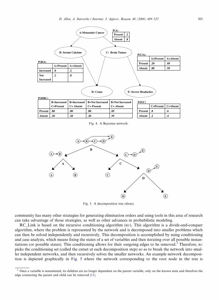
picks the conditioning set (called the cutset at each decomposition step) so as to break the network into smal-ler independent networks, and then recursively solves the smaller networks. An example network decomposi-tion is depicted graphically in Fig. 5 where the network corresponding to the root node in the tree is

2 Once a variable is instantiated, its children are no longer dependent on the parent variable, only on the known state and therefore theedge connecting the parent and child can be removed [11].


decomposed by conditioning on the variable B. Once B is instantiated the edges between B! C and B! E

are removed, resulting in two independent networks (one containing the variables {A,B} and the other con-taining the variables {C,D,E}). This decomposition structure is known as a decomposition tree (dtree). Moreformally, a dtree and the variables in the cutset are defined as:

Definition 1 (cf. [11]). A dtree for a Bayesian network is a full binary tree, the leaves of which correspond tothe network conditional probability tables (CPTs). If a leaf node t corresponds to a CPT /, then vars(t) isdefined as the variables appearing in CPT /. For an internal node t, with left child tl and right childtr; varsðtÞ ¼

defvarsðtlÞ [ varsðtrÞ.

Definition 2. The cutset of internal node t in a dtree is: cutsetðtÞ ¼defvarsðtlÞ \ varsðtrÞ � acutsetðtÞ, where acu-

tset(t) is the union of cutsets associated with ancestors of node t in the dtree.

It turns out that many of the subnetworks generated by this decomposition process need to be solved multi-ple times redundantly, allowing the results to be stored in a cache after the first computation and then subse-quently fetched during further computations. Specifically, if we define the context as in Definition 3, thencaches can be indexed by instantiations of the variables in the context, as any computation done under thesame context instantiation will produce equivalent results.

Definition 3. The context of node t in a dtree is: contextðtÞ ¼defvarsðtÞ \ acutsetðtÞ.

This ability to either cache or recompute computations allows RC to be an any-space algorithm, meaningit can run using any amount of memory. When less than the full amount of memory is used, RC must deter-mine how to best use the available memory (i.e. which computations to store in the caches and which torecompute) [3–5]. Given the above definitions, the pseudocode shown in Algorithms 1 and 2 will computethe probability of evidence, Pr(e) for the input network. A more through description of the algorithm canbe found in [11,3,5].

Algorithm 1 RC(t): Returns the probability of evidence e recorded on the dtree rooted at t

1: if t is a leaf node then2: return LOOKUP(t)3: else4: y recorded instantiation of context(t)5: if cache?(t) and cachet[y] 5 nil then6: return cachet[y]7: else8: p 09: for instantiations c of uninstantiated vars in cutset(t) do

10: record instantiation c11: p p + RC(tl)RC(tr)12: un–record instantiation c13: when cache?(t),cachet[y] p14: return p

Algorithm 2 LOOKUP(t)

/ CPT of variable X associated with leaf t

if X is then

x recorded instantiation of Xu recorded instantiation of X’s parentsreturn /(x|u) // /(x|u) = Pr(x|u)

else

return 1

Gp1 Gm1

P1

Gp2 Gm2

P2

Gp3 Gm3

P3

Gp1 Gm1

P1

Gp2 Gm2

P2

Gp3 Gm3

P3

Gp1 Gm1

P1

Gp2 Gm2

P2

Gp3 Gm3

P3

Sp1 Sm1

Sp2 Sm2

Sp3 Sm3

Father Mother

Child

Pedigree Bayesian Network

F M

C

Fig. 6. A pedigree and its corresponding Bayesian network.


3. Modeling linkage analysis with Bayesian networks

The following description is the method both SUPERLINK and RC_Link use to map the genetic linkageanalysis problem to a Bayesian network [15] and is currently one of the more common, however this is not theonly possible mapping [22]. During this discussion we will refer to the simple example in Fig. 6. The left side ofthe figure shows a simple pedigree containing three people (a father, mother, and child). The right side showsthe corresponding Bayesian network, assuming three loci are being modeled.

To model the problem as a Bayesian network, for each person in the pedigree and for each locus (geneticmarker or gene) being modeled, two random variables will be created called Gpi and Gmi, where i refers to thelocus. These represent the genotype of the individual (one models the paternal genotype variable and the otheris the maternal).3 For example if the gene we are interested in appears on the first pair of chromosomes, thenGpi models the value that the gene on the chromosome inherited from the father and Gmi models the valuefrom the other chromosome in the pair. In addition, a third variable Pi will be created which representsthe phenotype, or the observable outcome of the genotype. Edges will be added from each of the two genotypevariables to the phenotype variable, as the phenotype is a direct effect of the genotype. This mapping may bedeterministic (e.g. the AO blood genotype has the A phenotype) or may be probabilistic (e.g. a person mayhave the genotype for a disease, but only show symptoms with some probability). For the genetic linkage anal-ysis domain, the input specifies the genotype to phenotype mapping for each locus. Additionally, for thosegenotype variables associated with founders (i.e. genotype variables which do not have any parents in the net-work), their prior probabilities are also contained in the input.4

For people which are not founders (i.e. people who have parents included in the pedigree) we will create twoselector variables for each locus (Spi and Smi), which determine if the person inherits their parent’s paternalgenotype or their parent’s maternal genotype at that particular locus. One of these selectors, Spi, is the pater-nal selector and therefore edges are added from both of the father’s genotype variables and from this selectorinto the child’s paternal genotype variable. The maternal selector, Smi, is likewise created along with edgesfrom the mother.

3 Note that many examples in this paper use binary variables for simplicity, however in general the variables are multi-valued.4 One of the most common input formats is described in the user manual for the LINKAGE tool at http://linkage.rockefeller.edu/soft/

linkage/ or also described for the Superlink tool at http://bioinfo.cs.technion.ac.il/superlink/.

http://linkage.rockefeller.edu/soft/linkage/

http://linkage.rockefeller.edu/soft/linkage/

http://bioinfo.cs.technion.ac.il/superlink/


An example CPT for a nonfounder genotype variable is seen in Fig. 7. From this figure it can be seen thatthe selector variable simply selects which parent genotype to copy. In the figure, if S = 1 the child inherits theparent’s paternal genotype value and if S = 2 they inherit the maternal.

There are additional edges between consecutive paternal selectors and consecutive maternal selectors. Thesemodel the fact that if the preceding locus inherits from either the paternal or maternal haplotype (the paternalhaplotype is simply the set of paternal genotype variables, and similarly the maternal haplotype is the set ofmaternal genotype variables), then the current locus will also inherit from that haplotype, unless a recombi-nation event occurs. Therefore, a recombination occurs when the state of two consecutive selector variablesdiffer.

The selector for the first locus simply has a 50% chance of being in state 1 and similarly a 50% chance ofbeing in state 2. For selectors with parents, their CPTs contain the form shown in Fig. 8, where 1 � r is thecorresponding recombination fraction from h. These CPTs intuitively specify that with probability r the pro-cess will copy from the same haplotype as the preceding locus and with probability 1 � r a recombinationevent will occur.

After the pedigree is modeled by a Bayesian network, the next step is to compute the likelihood of theknown genotype and phenotype evidence for a given pedigree and set of recombination fractions. In Bayesiannetwork terminology, we would create a Bayesian network BN1 based on the pedigree, P, and h, then assertthe evidence e, and finally compute the probability of evidence Pr(e). To compute the likelihood for different h

vectors, we can modify the appropriate CPT parameters for each different vector, and for each compute Pr(e).Similarly, we can compute the LOD score by taking the log of (Pr(e|BN1) divided by Pr(e|BN2)), where BN2 iscreated from P and h with hi = 0.5.

Currently, many pedigrees of interest create Bayesian networks which are very challenging computation-ally. They can require significant amounts of memory (sometimes as much as 20 or 30 GB) using standard

Gp Gm

G

S=2S=1

1.0

0.0

Gm=2

1.0

0.0

Gm=1

Gp=2

0.0

1.0

Gm=2

0.0

1.0

Gm=1

Gp=1 Gp=2Gp=1

1.0

0.0

Gm=2

0.0

1.0

Gm=1

G=2

G=1

Gm=2Gm=1

1.00.0

0.01.0

P(G|S,Gp,Gm)

S

InterpretationS=1 implies G=GpS=2 implies G=Gm

Fig. 7. An example CPT for a nonfounder.

G

r

1-r

S1=2

1-r

r

S1=1

S2=2

S2=1

P(S2|S1)

S1

G

S2

Fig. 8. Format for a selector CPT.


algorithms and also can take hours to compute the probabilities [2,14]. These networks are also very large, forexample one network with 57 people and 43 loci contained 10,965 variables. Even more important in deter-mining the computational difficulty is the connectivity of the generated networks.

The Bayesian networks produced can be very challenging, however they also contain a significant amountof determinism. This means that the CPTs contain many zeros and ones (for example the CPTs for nonfound-er genotypes deterministically copy one of the two parent genotypes based on the selector, see Fig. 7). Theimplications of this are that when some variables have known values, then other variables can sometimesbe determined (or learned). We have previously shown that this can be taken advantage of and that it can leadto significant computational speedups [2,8]. This is especially true for probabilistic inference algorithms whichwork using variable conditioning such as recursive conditioning.

The past few years have shown remarkable improvement on the capabilities of genetic linkage analysisusing Bayesian networks. Many of the networks which were previously too costly to do inference on cannow be solved using newly developed techniques, however there are still many networks which are challenging[14]. Therefore, exploring additional techniques to further extend the boundary of which networks are com-putationally feasible is important.

4. Preprocessing

This section presents simplification techniques for preprocessing Bayesian networks in order to make infer-ence more tractable while maintaining the ability to compute the correct probabilities. Some of these are usedby other probabilistic inference or genetic linkage tools, while others are novel techniques for network simpli-fication. The preprocessing methods are broken down into two groups, those which are applicable to anyBayesian network and those which are dependent on the domain of genetic linkage analysis. Following thesimplification technique descriptions, Section 4.3 will discuss the applicability and effectiveness of the differenttechniques.

4.1. Simplification techniques for Bayesian networks

This section presents seven techniques which are useful for any Bayesian network inference algorithm. Thefirst two we present (State Removal and Classical Pruning) are previously existing techniques [15,32,33]. Thesubsequent five simplifications (Independent Variables, Chain Variables, Single-Child Founder Removal,Irrelevant Edges, and Variable Equivalence) are all new techniques for network simplification.

4.1.1. State removal

A Bayesian network normally has the property that for all parent instantiations the probabilities of thechild states conditioned on the parent instantiation must sum to 1.0. For example, in the CPT on the left sideof Fig. 9 we note that each column sums to 1.0. Our modeling of the networks presented in the previous sec-tion also contains this property, however once the network is generated we will relax this requirement. Spe-cifically, when either the evidence or other simplification techniques determine a state is not possible we

A B

C

1.00.00.00.0C=2_2

1.0

0.0

A=a1B=b2

1.0

0.0

A=a2B=b1

C=1_2

C=1_1

A=a2B=b2

A=a1B=b1

0.00.0

0.01.0

P(C|AB)

A B

C

1.0

A=a1B=b2

1.0

A=a2B=b1

C=1_2

A=a2B=b2

A=a1B=b1

0.00.0

P(C|AB)Evidence C=1_2

Fig. 9. An example of State Removal.


will remove it. An example of such a simplification can be seen on the right side of Fig. 9, where two states ofvariable C were removed based on the evidence C = 1_2, leading to CPT columns which do not sum to 1.0. Itshould be noted that the initial network is a valid Bayesian network, and hence represents a valid joint prob-ability distribution, and that our modified network is probabilistically equivalent to the original network plusthe included evidence. The removal of impossible states means the inference algorithm has to look at fewerpossible instantiations, allowing them to run faster, although they can then only answer queries with regardto that evidence.

One specific method for detecting states which will always result in a probability of 0.0 and can thereby beremoved is value elimination [15]. An example of this is if X can be in the states {x1,x2,x3,x4} and all entriesin any CPT containing X = x1 contain the probability value of 0 (i.e. Pr(X = x1,Y,Z) = 0.0 for all values of Y

and Z). In this case, x1 can be removed from the domain of variable X, because it is never a valid state. If weexamine the left side of Fig. 9, but instead of the evidence in the figure let us assume the evidence is C = 1_1.We can then remove the last two rows of the CPT based on our State Removal simplification. Once this isdone, if we look at Pr(A = a2,B,C = 1_1) for every value of B the probability is equal to 0.0. Therefore,we can remove the state a2 from the domain of A. Note that we can eliminate states of variables based onany table they are a part of. In this case, we removed a state from variable A, however the table used wasthe CPT for variable C. The changes will also not only affect the current table, but will change every othertable the variable is a part of, as they also will be updated when the states are removed. Specifically, if weremove the state a1 from A, then every parent or child instantiation which contains a1 will also be removed,possibly leading to further simplifications. In this example, we could additionally remove the state b2 from Bin a similar fashion to that of a2. Since both A and B were binary variables which became unary variables, theynow have a known value, which will allow classical pruning to further simplify the network structure.

4.1.2. Classical pruning

We define classical Bayesian network pruning as removing leaf nodes that are not part of the evidence orquery [32] and removing edges outgoing from observed nodes [33]. We have already seen the removal of edgesfrom observed nodes during the discussion on conditioning. Leaf nodes without evidence can be removedsince in any probability calculation on the network that variable’s contribution will be a multiplication by1.0. To see this let us examine the Lookup(t) function in Algorithm 2. By definition, variables which onlyappear in a leaf node do not appear in any cutsets, so when Lookup is called the variable will be uninstantiatedunless it has evidence. Therefore, for leaf nodes without evidence, Lookup will always return 1.0. By examiningthe remainder of the algorithm it can be seen that the probability value computed will therefore be the same ifthose leaf variables with no evidence are removed.

Initially we may have many leaf nodes without evidence, for example every phenotype variable is a leaf.Hence, any phenotype variable which does not have evidence associated with it can be pruned. This could alsothen lead to its parents becoming leaf nodes allowing them to possibly be pruned.

The second rule, removing outgoing edges from observed variables, is not initially applicable. The evidenceprovided for the genetic linkage domain is usually all on phenotype variables, which are all leaf nodes andtherefore do not have outgoing edges. However based on the determinism and other simplifications, additionalevidence can be learned and then this rule may be useful and allow for network structure simplification. Anexample of this can be seen in Fig. 10, where we have evidence on the phenotype variable that it is homozygous(i.e. that both genotype variables are equal to one another). The evidence specifies that P = 1_1 and based onthe CPT we see that therefore Gp and Gm must both be in state 1. This additional evidence then allows clas-sical pruning to remove outgoing edges from Gp and Gm, in this case removing six edges and making P anindependent variable.

4.1.3. Independent variables

In the example in Fig. 9, the variables A, B, and C became independent variables, meaning that they do nothave any edges coming in or departing from them. Likewise, in Fig. 10, variable P became independent. Inthese cases, if the variables have no evidence associated with them, then since they are leaf nodes they canbe removed. However if they do have evidence, it is clear that the lack of edges means that they are indepen-dent of the remainder of the network. Therefore they only contribute a constant to any probability calculation

Gp Gm

P

1.00.00.00.0P=2_2

1.0

0.0

Gp=1Gm=2

1.0

0.0

Gp=2Gm=1

P=1_2

P=1_1

Gp=2Gm=2

Gp=1Gm=1

0.00.0

0.01.0

P(P|Gp,Gm)

Evidence P=1_1

Gp=1 Gm=1

P=1_1

Fig. 10. An example of classical pruning and homozygous evidence.


on the network. Note that this evidence could be in the form of standard evidence where we know which statethe variable is in, or it could be in the form of states which have been removed (i.e. negative evidence). In gen-eral, any independent variable X can be removed from the network and replaced by the constant c, wherec ¼

Pxi2X PrðxiÞ.

There may be a significant number of these independent variables, depending on the network structure andthe simplification techniques used. All these constants can therefore be multiplied together to form a singleconstant, rather than maintaining each individually. One additional note is that if these variables are queryvariables or if their network parameters are to be changed, then extra bookkeeping must be used to allowfor those to occur prior to the variables’ removal.

4.1.4. Chain variables

Another type of variable which can be preprocessed are those whose indegree is less than or equal to 1 andwhose outdegree is equal to 1. We will call these variables chain variables, as they participate in a ‘‘ChainStructure.’’ This novel technique can be seen in Fig. 11. The variables B, C, and E are all chain variablesand therefore can be eliminated. To eliminate the variable B, which has parent A and child C, we multiplythe CPT for variable B and the CPT for variable C together, resulting in a table over variables A, B, andC. We then sum out the variable B, leaving a table over variables C and A, which will then be the new

A

B

C

D

EF

A

D

F

D

F

Fig. 11. An example of chain variables.


CPT for variable C. As a result of the multiplication and summation, if we assume all the variables are binary,one example entry in this table for {c1|a1} would contain the result of {c1|b1} * {b1|a1} + {c1|b2} * {b2| a1}.

The second figure shows the network after this is done for B, C, and E (Note that the CPTs for A and D arenow different than in the first figure). Looking at this new network we see that the removal of E has nowcaused A to also become a chain variable and so it can also be eliminated, resulting in the third network.We see that by preprocessing these variables the resulting network has fewer variables, and usually this processwill not increase the complexity of inference and it will always maintain the correct computations. We notethat by removing the variables we lose the ability to compute marginals over them, however for genetic linkageanalysis we are usually only interested in computing the probability of evidence. We also need to be careful ifwe want to update the network parameters for any chain variable or its child, as once the tables are multipliedtogether it is harder to determine how to update them. Therefore, variables whose parameters will be changedshould either not be eliminated using this rule, or additional bookkeeping must be used to determine how toupdate the parameters.

4.1.5. Single-child founder removal

Removing chain variables which are roots is a special case of relevance reasoning [25]. Another easilyexploitable example of relevance reasoning in genetic networks are pedigree founders (those with no parentinformation in the pedigree) which only have a single child (note that this refers to the person having a singlechild, and not to a variable having a single child as we saw for chain variables). See Fig. 12 for an examplewhere we have one founder with two loci and a single child (we only show the corresponding genotype andselector variables for the child). These founders contain three variables for each locus: Gmi, Gpi, and Pi.The genotype variables each will have a single edge with a common child variable, however they are not chainvariables as they also have an edge to the phenotype variable. If the phenotype is unknown, then it will beremoved by classical pruning and the genotypes will be removed because they become chain variables. How-ever if the phenotype is known, the previous simplifications will not help. As a group those three variables onlycontain a single child, and therefore they form a nuisance graph, and can be simplified [25]. One method forsimplifying them is to multiply the CPTs for the four variables and then sum out the three variables associatedwith the founder, leaving a valid CPT for the child variable. We can apply this technique to each locus, there-fore the end result will be that all variables associated with the founder will be removed, as seen in Fig. 12where all six founder variables have been merged into the child’s genotype CPTs.

Gp1 Gm1

P1

G1FounderRemoval

Gp2 Gm2

P2

G2

S

SG1

G2

S

S

Founder, locus 1

Founder, locus 2 Child Child

Fig. 12. An example of removing a founder with only one child.


The notion of relevance reasoning and nuisance graphs are previously known simplifications which are use-ful for general probabilistic inference. The contribution we make to this is in the realization of how frequentlythese occur in the genetic linkage analysis domain, and that applying this simplification allows these compu-tations to be done a single time instead multiple times.

4.1.6. Irrelevant edges

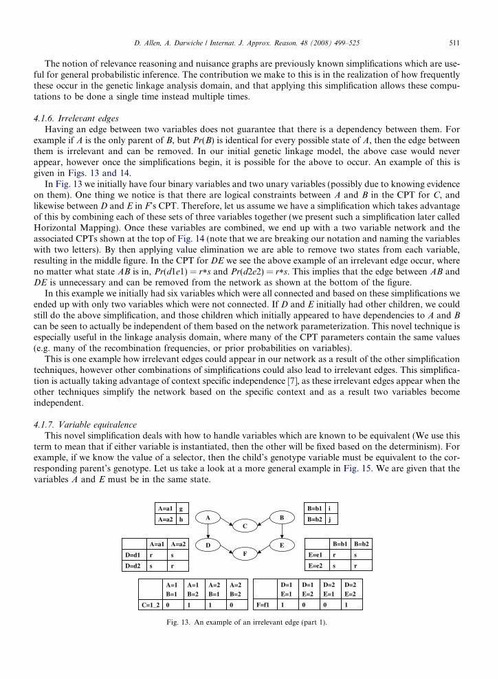
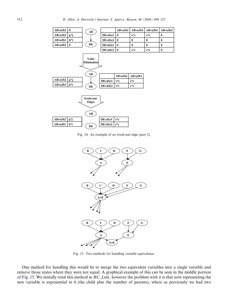
Having an edge between two variables does not guarantee that there is a dependency between them. Forexample if A is the only parent of B, but Pr(B) is identical for every possible state of A, then the edge betweenthem is irrelevant and can be removed. In our initial genetic linkage model, the above case would neverappear, however once the simplifications begin, it is possible for the above to occur. An example of this isgiven in Figs. 13 and 14.

In Fig. 13 we initially have four binary variables and two unary variables (possibly due to knowing evidenceon them). One thing we notice is that there are logical constraints between A and B in the CPT for C, andlikewise between D and E in F’s CPT. Therefore, let us assume we have a simplification which takes advantageof this by combining each of these sets of three variables together (we present such a simplification later calledHorizontal Mapping). Once these variables are combined, we end up with a two variable network and theassociated CPTs shown at the top of Fig. 14 (note that we are breaking our notation and naming the variableswith two letters). By then applying value elimination we are able to remove two states from each variable,resulting in the middle figure. In the CPT for DE we see the above example of an irrelevant edge occur, whereno matter what state AB is in, Pr(d1e1) = r*s and Pr(d2e2) = r*s. This implies that the edge between AB andDE is unnecessary and can be removed from the network as shown at the bottom of the figure.

In this example we initially had six variables which were all connected and based on these simplifications weended up with only two variables which were not connected. If D and E initially had other children, we couldstill do the above simplification, and those children which initially appeared to have dependencies to A and B

can be seen to actually be independent of them based on the network parameterization. This novel technique isespecially useful in the linkage analysis domain, where many of the CPT parameters contain the same values(e.g. many of the recombination frequencies, or prior probabilities on variables).

This is one example how irrelevant edges could appear in our network as a result of the other simplificationtechniques, however other combinations of simplifications could also lead to irrelevant edges. This simplifica-tion is actually taking advantage of context specific independence [7], as these irrelevant edges appear when theother techniques simplify the network based on the specific context and as a result two variables becomeindependent.

4.1.7. Variable equivalence

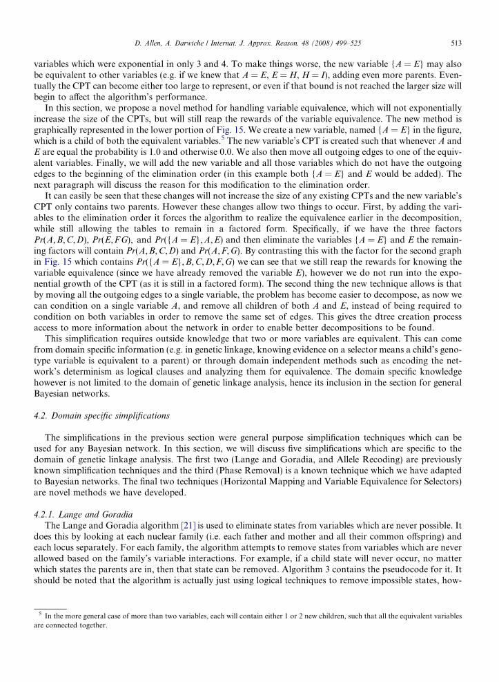
This novel simplification deals with how to handle variables which are known to be equivalent (We use thisterm to mean that if either variable is instantiated, then the other will be fixed based on the determinism). Forexample, if we know the value of a selector, then the child’s genotype variable must be equivalent to the cor-responding parent’s genotype. Let us take a look at a more general example in Fig. 15. We are given that thevariables A and E must be in the same state.

1

A=1B=2

0

A=1B=1

01C=1_2

A=2B=2

A=2B=1

A

D

B

E

C

F

0

D=1E=2

1

D=1E=1

10F=f1

D=2E=2

D=2E=1

hA=a2

gA=a1

jB=b2

iB=b1

rsD=d2

s

A=a2

r

A=a1

D=d1

rsE=e2

s

B=b2

r

B=b1

E=e1

Fig. 13. An example of an irrelevant edge (part 1).

AB

DE

0r*ss*r0DE=d2e2

0000DE=d2e1

0

r*s

AB=a1b2

0

0

AB=a1b1

00DE=d1e2

0

AB=a2b2

s*r

AB=a2b1

DE=d1e1

0AB=a2b2

h*iAB=a2b1

g*j

0

AB=a1b2

AB=a1b1

r*ss*rDE=d2e2

r*s

AB=a1b2

s*r

AB=a2b1

DE=d1e1

ValueElimination

h*iAB=a2b1

g*jAB=a1b2

AB

DE

Irrelevant Edges

s*rDE=d2e2

r*sDE=d1e1

h*iAB=a2b1

g*jAB=a1b2

AB

DE

Fig. 14. An example of an irrelevant edge (part 2).

A

B

E

GFDC

A=E

B GFDC

A

B

E

GFDC

A=E

Fig. 15. Two methods for handling variable equivalence.


One method for handling this would be to merge the two equivalent variables into a single variable andremove those states where they were not equal. A graphical example of this can be seen in the middle portionof Fig. 15. We initially tried this method in RC_Link, however the problem with it is that now representing thenew variable is exponential in 6 (the child plus the number of parents), where as previously we had two


variables which were exponential in only 3 and 4. To make things worse, the new variable {A = E} may alsobe equivalent to other variables (e.g. if we knew that A = E, E = H, H = I), adding even more parents. Even-tually the CPT can become either too large to represent, or even if that bound is not reached the larger size willbegin to affect the algorithm’s performance.

In this section, we propose a novel method for handling variable equivalence, which will not exponentiallyincrease the size of the CPTs, but will still reap the rewards of the variable equivalence. The new method isgraphically represented in the lower portion of Fig. 15. We create a new variable, named {A = E} in the figure,which is a child of both the equivalent variables.5 The new variable’s CPT is created such that whenever A andE are equal the probability is 1.0 and otherwise 0.0. We also then move all outgoing edges to one of the equiv-alent variables. Finally, we will add the new variable and all those variables which do not have the outgoingedges to the beginning of the elimination order (in this example both {A = E} and E would be added). Thenext paragraph will discuss the reason for this modification to the elimination order.

It can easily be seen that these changes will not increase the size of any existing CPTs and the new variable’sCPT only contains two parents. However these changes allow two things to occur. First, by adding the vari-ables to the elimination order it forces the algorithm to realize the equivalence earlier in the decomposition,while still allowing the tables to remain in a factored form. Specifically, if we have the three factorsPr(A,B,C,D), Pr(E,FG), and Pr({A = E},A,E) and then eliminate the variables {A = E} and E the remain-ing factors will contain Pr(A,B,C,D) and Pr(A,F,G). By contrasting this with the factor for the second graphin Fig. 15 which contains Pr({A = E},B,C,D,F,G) we can see that we still reap the rewards for knowing thevariable equivalence (since we have already removed the variable E), however we do not run into the expo-nential growth of the CPT (as it is still in a factored form). The second thing the new technique allows is thatby moving all the outgoing edges to a single variable, the problem has become easier to decompose, as now wecan condition on a single variable A, and remove all children of both A and E, instead of being required tocondition on both variables in order to remove the same set of edges. This gives the dtree creation processaccess to more information about the network in order to enable better decompositions to be found.

This simplification requires outside knowledge that two or more variables are equivalent. This can comefrom domain specific information (e.g. in genetic linkage, knowing evidence on a selector means a child’s geno-type variable is equivalent to a parent) or through domain independent methods such as encoding the net-work’s determinism as logical clauses and analyzing them for equivalence. The domain specific knowledgehowever is not limited to the domain of genetic linkage analysis, hence its inclusion in the section for generalBayesian networks.

4.2. Domain specific simplifications

The simplifications in the previous section were general purpose simplification techniques which can beused for any Bayesian network. In this section, we will discuss five simplifications which are specific to thedomain of genetic linkage analysis. The first two (Lange and Goradia, and Allele Recoding) are previouslyknown simplification techniques and the third (Phase Removal) is a known technique which we have adaptedto Bayesian networks. The final two techniques (Horizontal Mapping and Variable Equivalence for Selectors)are novel methods we have developed.

4.2.1. Lange and Goradia

The Lange and Goradia algorithm [21] is used to eliminate states from variables which are never possible. Itdoes this by looking at each nuclear family (i.e. each father and mother and all their common offspring) andeach locus separately. For each family, the algorithm attempts to remove states from variables which are neverallowed based on the family’s variable interactions. For example, if a child state will never occur, no matterwhich states the parents are in, then that state can be removed. Algorithm 3 contains the pseudocode for it. Itshould be noted that the algorithm is actually just using logical techniques to remove impossible states, how-

5 In the more general case of more than two variables, each will contain either 1 or 2 new children, such that all the equivalent variablesare connected together.


ever we classify it as domain specific due to the choice of which variables to examine (i.e. it needs to knowwhich variables are part of each nuclear family, but otherwise the techniques involved are general purposesimplifications).

Algorithm 3 Lange and Goradia Algorithm

1: for each nuclear family do2: for each person do3: Reduce genotype states based on known phenotypes4: for each possible configuration of mother–father genotypes do5: Determine all 8 valid children types6: if all children have at least 1 valid configuration then7: Mark the mother– father states as saved8: Mark any child state which is valid for this as saved9: for each person do

10: Remove states not marked as saved11: Repeat until nothing new is learned

4.2.2. Allele recodingAllele recoding was presented in [26], and was adapted to Bayesian networks in [14]. The basic idea of this

simplification is that sometimes it is not possible to distinguish two states for a given variable (an occurrenceof this is when no descendants of a person have that state as a known phenotype). More formally, ‘‘an allele isdefined to be transmitted if the following two conditions are fulfilled: (i) the allele appears in the ordered geno-type list of a typed descendant D of P, as inherited from; (ii) there is some path from P to D containing onlyuntyped descendants in the pedigree, namely, D is the nearest typed descendant of P on that path. The remain-ing alleles are defined to be non-transmitted.’’ [14] For each variable, the non-transmitted states are indistin-guishable and can be merged into a single state, taking care to maintain the appropriate inheritance properties[26]. The end result of this simplification is that the variables may have fewer states, and hence are easier to docomputations on. We refer the reader to [14] for the actual implementation details, as they present a simplealgorithm for detecting the transmitted states.

4.2.3. Phase removal

Since founders do not have any information about ancestors, it turns out that their paternal and maternalgenotype variables cannot be differentiated. This leads to what is known as phase removal, which detects twoequivalent classes of instantiations and removes one of them [19]. However there are multiple ways of reducingit and the method chosen is significant in determining how beneficial it is. We first define the simplificationusing an example and then present a novel method for taking advantage of it in the context of Bayesiannetworks.

Fig. 16 contains a three locus example with a founder (the six genotype variables in the upper left) and threechildren (only their genotype and selector variables associated with this parent are depicted). We first define a

G

G

G

G G

G G

G G G

G

G

S

S

S

G

G

G

S

S

S

S

S

S

Fig. 16. Phase removal simplification.


function InvertPhase(Founder,Child1,Child2 . . . ), which for any complete instantiation inverts the state ofeach child’s selector variables (i.e. if it was copying the left parent genotype it will copy the right and viceversa) and also it will swap the founder genotypes (i.e. the founder’s paternal variable will take on the statethe maternal variable had and vice versa).

For any valid instantiation of the variables, the instantiation produced by InvertPhase() will also exist andfurthermore both instantiations will be equally likely. This is true since none of the selector variables associ-ated with the child of a founder can contain any evidence (as two genotype variables cannot be distinguishedwithout additional information from ancestors, which founders do not have). Therefore, since no evidence isknown on the selectors their inverted state is also possible and equally likely. Likewise, since founder genotypevariables cannot be distinguished, any state possible for the paternal genotype must also be possible (andequally likely) for the maternal and vice versa. Therefore, for any instantiation of the variables, the instanti-ation produced by InvertPhase() will also be valid and will be equally likely.

Based on the fact that for each instantiation there is a second one with equal probability (with a 1 to 1 cor-respondence), the total number of possible instantiations for the network variables can be reduced by 2F,where F is the number of founders in the network. Taking advantage of this can lead to significant perfor-mance enhancements, however we must first determine how to remove the superfluous phases and updatethe probability of those remaining.

There are a number of different possible methods for doing this in a Bayesian network and differing meth-ods will have varying improvements to the inference time. One simple method is to simply pick any singleselector associated with each founder and set it to be in one of its states (as both are valid) and then doublethe probability of that occurrence. It should be apparent that setting the evidence on one of the selectors willthen not allow the InvertPhase() function to work (as one of the phases will now be invalidated due to theevidence).

However, based on our experiments with a few additional methods, the one which experimentally seemed towork best was the following. We first pick one of the founder’s loci to remove the phase at. We pick this locusby first choosing any which are known to be heterozygous. Whether or not any locus have this property wewill then break ties by choosing the locus with the maximum number of child variables with evidence and fur-ther break ties by choosing the one with the maximum number of child variables (note that normally eachlocus would have the same number of children, however due to other simplifications some of the child’s vari-ables may have been removed).

Once the locus to simplify is chosen, we will remove the phase there. If the locus is heterozygous (for exam-ple it must be either 1_2 or 2_1) then we can merge these variables together using the next simplification (Hor-izontal Mapping) and then remove one of the two states and double the probability of the other (e.g. removestate 1_2 and double the probability of 2_1). If the founder is not a known heterozygous variable, then we lookto see if any of the children have known genotype variables. If so, we set evidence on the corresponding selec-tor and double the probability (e.g. we can set the selector to always copy the left genotype, and since thechild’s genotype is known, say for example it is in state 1, then all valid parent instantiations must have 1as the left genotype). Finally, if no children have known genotypes we can still take advantage of the phaseremoval by again combining the founders genotype variables and then removing the phase there (e.g. for everystate i_j where i 5 j, remove the state j_i and double the probability of i_j).

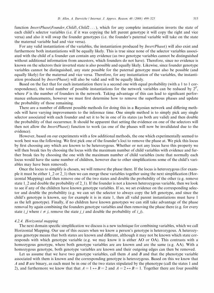
4.2.4. Horizontal mapping

The next domain specific simplification we discuss is a new technique for combining variables, which we callHorizontal Mapping. Our use of this occurs when we know a person’s genotype is heterozygous. A heterozy-gous genotype means that both states are known and different, although it may not be known which state cor-responds with which genotype variable (e.g. we may know it is either AO or OA). This contrasts with ahomozygous genotype, where both genotype variables are are known and are the same (e.g. AA). With ahomozygous genotype, both genotype variables are known and their outgoing edges can then be removed.

Let us assume that we have two genotype variables, call them A and B and that the phenotype variableassociated with them is known and the corresponding genotype is heterozygous. Based on this we know thatA and B are binary, as each must be in one of the two states stipulated by the phenotype (call the states 1 and2), and furthermore we know that that A = 1 M B = 2 and A = 2 M B = 1. Together there are four possible


configurations of these variables (1_1, 1_2,2_1, and 2_2), however only two of them are heterozygous. Theproblem is that with the variables separate, neither variable can have any state removed, as every state is stillpart of some valid instantiation. Therefore, we combine those variables into a single variable with four states,which then allows us to remove the two non-heterozygous states.

This simplification also enables the decomposition process to realize that setting the state of one of thesevariables actually removes all the outgoing edges from both (as one variable determines the other and viceversa). Also, since there are only two variables, the new CPT will not grow too large, as was seen with thevariable equivalence simplification. Therefore, this simplification enables the inference algorithm to skipimpossible instantiations (e.g. those which contain 1_1 and 2_2) and also further empowers the decompositionprocess with additional information.

4.2.5. Variable equivalence for selectorsOur final domain specific simplification is a novel technique for determining equivalence between variables

in this domain and then advantageously using that to simplify our network. Let us examine Fig. 17. We seethat the parent genotype is heterozygous (having states 1_2 or 2_1). Likewise we are given three children whichhave their associated selector variable and a known genotype variable.

By using horizontal mapping we will assume that the parent variables are merged into a single variable withtwo states. Let us examine the case where it is in the state 1_2. From this we see that the first two selectors mustcopy the 1 from the left genotype variable and the other must copy the 2 from the right. Likewise, if we exam-ine the state 2_1, again all three selectors are determined. In fact, given evidence on any one of the three selec-tors or the parent determines the states of all the others. Therefore, we see that the selectors are not in factindependent and in fact are very tightly coupled, regardless of the fact that the edge paths between themgo through multiple other variables (i.e. the shortest path between them is to go from the selector to the knownchild genotype, to an unknown parent genotype, back to another known child genotype, and finally to anotherselector).

This relationship between the selectors and parent genotype variable can help the decomposition process. Inorder to take advantage of this, we rely on our method for Variable Equivalence in the previous section. Spe-cifically, whenever we have a heterozygous parent, call it X, (e.g. we might know this through evidence on thephenotype) we create an equivalence mapping between X and every selector Y which is associated with aknown child genotype variable. As mentioned in the Variable Equivalence section, this empowers the decom-position process with the knowledge about the interrelationship, while still allowing the CPTs to remain in afactored form.

4.3. Simplification technique applicability and effectiveness

Before moving on to the last set of simplifications, those relating to the recursive conditioning algorithm,we will first address the applicability and effectiveness of some of the novel techniques already discussed.

One advantage of these simplification techniques is their reduction of recalculations. Three importantplaces where recalculations are taking place are during each calculation of the probability of evidence,between subsequent queries with different network parameterizations, and when searching for a good net-work decomposition. By preprocessing our networks with these simplification techniques we can remove

G

G G

GS

GS S

1_22_1

1 21

Fig. 17. Selector variable equivalence.

Table 1Number of variables in networks after simplifications

Network Expected size Actual size

EA7 3570 422EA8 4590 442EA9 9435 745EA10 9690 764EA11 10,965 841

1 752 2227 2140 4239 1720 64013 1680 55218 1740 61919 1285 52420 749 22923 777 20125 2155 54830 2195 62931 2155 66233 2315 38034 2140 48437 1530 31738 1020 35739 2140 44940 1740 58841 2155 48242 763 23744 1820 48350 1020 28751 2300 627


some of the recalculations by simply doing computations a single time instead of multiple times during thequeries or decomposition search. Some examples of this are the Independent Variables and Chain Variablessimplifications. Many standard inference algorithms would readily handle these types of variables, howeverby simplifying them once during a preprocessing step, we allow our algorithms to not recompute the relevantvalues multiple times. An example would be the Independent variables, which simply contribute a constantvalue to the probability query. By preprocessing, we compute this constant once, and then can use it duringmultiple queries under different parameterizations without recomputing it. Additionally, when we search fora good decomposition, which will be addressed in Section 6, we have already removed these variables sim-plifying our search. This reduction of recalculations is the main advantage of the Independent Variable andChain Variable techniques. The Single-Child Founder Removal technique also assists in reducing recalcula-tions, and in addition can sometimes assist in simplifying the network structure allowing other techniques,such as Chain Variables or Irrelevant Edges to be used. Table 1 shows the size of some networks after thesimplification techniques were run and the full size under no simplifications (These networks will be furtherdiscussed in the results in Section 7). As can be seen, the preprocessing steps can greatly reduce the size ofthe network.

The different techniques can have varying levels of effectiveness, and are especially dependent on theamount of evidence known in the network (e.g. genetic marker readings, disease affection status, etc.).Fig. 18 depicts the speedup on a few networks from three of the simplification techniques.6 In the log-plot,the three lines represent the ratio of the time without a given simplification to the time with all simplifications.In these instances, it can be seen that the Phase Removal and Variable Equivalence improved the inference

6 In order to compensate for the non-deterministic nature of the algorithm, the timings are all averaged over five runs.

0.1

1.0

10.0

100.0

1000.0

1 9 13 18 19 20 23 25 30 31 33 34 37 38 39 40 41 42 44 51Networks

Tim

e W

ithou

t Spe

cific

Sim

plifi

catio

ns /

Tim

e w

ith A

ll Si

mpl

ifica

tions

No PhaseRemovalNo HorizontalMerging (and noVar. Equiv.)

No VariableEquivalence

7

Fig. 18. Simplification technique effectiveness.


time, however by turning off the Horizontal Mapping (which also turns off the Variable Equivalence tech-nique) we saw the most slowdown. It should be noted here, that when one simplification technique is turnedoff, others (including those discussed in the next section) may partially compensate for the turned off tech-nique. For example, when variable equivalence is turned off, the decomposition search and skipping compu-tations may still take capture some of the additional instantiations with 0 probability.

In the next two sections we will further discuss simplification techniques which allow us to reuse computa-tions between queries and to search for good network decompositions.

5. Optimizing recursive conditioning

The last three simplifications are all novel and relate directly to the use of the recursive conditioning algo-rithm in our genetic linkage computations.

5.1. Skipping computations

The first of the RC based simplifications relates to skipping computations which will have no relevance tothe final result. If we examine Algorithm 1, we see on Line 11 that we recursively call RC on each child andmultiply the results together. Therefore, if the result on the left child is 0, there is no need to call RC on theright child, as no matter what the result is, it will be multiplied by 0. Hence when 0 is returned from the leftchild we can skip all the computations on the right. In some cases the result of this can dramatically affect theinference time. We remind you that the number of recursive calls is proportional to the time required to runRC. Table 2 shows the total number of recursive calls (and hence the time requirement) the algorithm wouldmake (labeled as expected), and then displays the actual amount that occurred based on this simplification(labeled Run 1). It also displays the ratio between these two values showing the proportion of actual callsto expected calls. It can be seen that this rule’s usefulness varies for each problem, however some of the

Table 2Experimental results displaying two simplifications (in number of recursive calls)

Network Expected Run 1 Run 2 Run 1Expected

Run 2Run 1

1 5.45E+07 5.03E+07 4.73E+07 0.92 0.947 3.84E+07 2.80E+07 2.63E+07 0.73 0.949 4.46E+08 2.57E+08 2.56E+08 0.58 0.9913 1.91E+08 1.68E+08 1.62E+08 0.88 0.9618 9.19E+06 6.93E+06 2.59E+06 0.75 0.3719 3.76E+07 2.88E+07 2.29E+07 0.77 0.8020 1.43E+08 6.70E+07 6.59E+07 0.47 0.9823 5.94E+06 2.29E+06 1.85E+06 0.38 0.8125 5.89E+07 3.97E+07 3.65E+07 0.68 0.9230 8.74E+06 6.50E+06 2.50E+06 0.74 0.3831 2.98E+08 1.89E+08 1.73E+08 0.63 0.9133 2.30E+06 1.43E+06 3.35E+05 0.62 0.2334 5.20E+07 4.11E+07 3.92E+07 0.79 0.9537 7.88E+08 7.96E+07 7.72E+07 0.10 0.9738 1.25E+10 3.94E+08 3.92E+08 0.03 1.0039 1.28E+07 8.47E+06 2.40E+06 0.66 0.2840 9.55E+07 6.92E+07 6.04E+07 0.72 0.8741 3.44E+07 2.40E+07 3.19E+06 0.70 0.1342 9.51E+07 5.76E+07 5.25E+07 0.61 0.9144 1.35E+09 2.19E+08 1.90E+08 0.16 0.8750 6.17E+12 2.02E+11 2.02E+11 0.03 1.0051 1.36E+09 6.72E+08 6.44E+08 0.49 0.96


networks only required 3% of the calls to be made, and every network had as least a small speedup based onthis optimization, which requires very little overhead to implement.

5.2. Caching results between computations

It is known that when doing multiple computations on the same network that many computations can bereused between different calls. However between each call changes are made in the form of either CPT param-eter changes or evidence changes. In classical algorithms it is difficult to determine which computations willbecome invalid due to these changes, however with RC it is easy. RC simply has to invalidate some correspond-ing cache values.

Specifically, given a dtree T, let us consider a change to a CPT parameter in the table associated with theleaf node X. Since RC only ever ‘‘passes’’ information up the dtree, we simply invalidate all cache entries whichare located at nodes corresponding to ancestors(X). Similarly, we note that if evidence is changed on a variablewhose CPT is located at leaf node Y, we can simply invalidate cache entries corresponding to ancestors(Y).This can be seen since setting the evidence on Y would only affect computations influenced by leaf Y (whichwe invalidate and would recompute) or computations where Y is a parent to another variable in which casethose computations would eventually be multiplied with an ancestor of Y, in which case any computationswhich contradict the evidence will be multiplied by a 0.

Table 2 contains the number of recursive calls for Run 1 and also those required during a second run, afterchanging the recombination frequencies during a maximum likelihood search. It can be seen from comparingthe Run 1 column with the Run 2 column how much time was saved due to those saved cache entries. Forexample, network 44 only required 13% of the calls in order to do the second computation as it required inthe first computation. Additionally, for the maximum likelihood search used in genetic linkage analysis, thesame parameters are repeatedly changed. Therefore, future runs during the search would require the samenumber of calls as shown in the Run 2 column.

In the future, it might also be possible to incorporate this information into the decomposition process, as ifthe changes are known a priori, dtrees may be constructed which specifically allow those changes while min-imizing the number of recomputed or invalidated cache entries.


5.3. Conditioning with a knowledge base

This simplification technique was explored in detail in [2], where it was shown that the combination of alogical knowledge base and conditioning algorithms could sometimes lead to significant timing improvements.This is due to the fact that as each variable is conditioned on, other variables may also be fixed based on thenetwork’s determinism. This technique captures many of the same simplifications as the State Removal tech-nique, however it is handled dynamically rather than as a static preprocessing step (as RC conditions on vari-ables in the cutset the technique dynamically learns the value of other variables, leading to simplifications lateron in the query). As we exploited additional determinism during the preprocessing phase, less remained in thefinal network for this technique to take advantage of. Therefore, the current implementation of RC_Link hasthis technique turned off by default, as its overhead versus its benefits can be significant based on the networkand its determinism, however is some instances the overhead is still outweighed by the time reduction.

6. Decomposition search

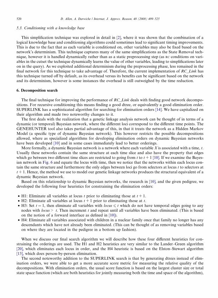
The final technique for improving the performance of RC_Link deals with finding good network decompo-sitions. For recursive conditioning this means finding a good dtree, or equivalently a good elimination order.SUPERLINK has a sophisticated algorithm for searching for elimination orders [14]. We have capitalized ontheir algorithm and made two noteworthy changes to it.

The first deals with the realization that a genetic linkage analysis network can be thought of in terms of adynamic (or temporal) Bayesian network, where the different loci correspond to the different time points. TheGENEHUNTER tool also takes partial advantage of this, in that it treats the network as a Hidden MarkovModel (a specific type of dynamic Bayesian network). This however restricts the possible decompositionsallowed, where as specialized algorithms for developing elimination orders on dynamic Bayesian networkshave been developed [10] and in some cases immediately lead to better orderings.

More formally, a dynamic Bayesian network is a network where each variable X is associated with a time, t.Usually these networks contain the same structure at each time slice and also have the property that edgeswhich go between two different time slices are restricted to going from t to t + 1 [10]. If we examine the Bayes-ian network in Fig. 6 and equate the locus with time, then we notice that the networks within each locus con-tain the same structure and furthermore the only edges between loci go from selectors at locus t to selectors att + 1. Hence, the method we use to model our genetic linkage networks produces the structural equivalent of adynamic Bayesian network.

Based on this relationship to dynamic Bayesian networks, the research in [10], and the given pedigree, wedeveloped the following four heuristics for constraining the elimination orders:

• H1: Eliminate all variables at locus t prior to eliminating those at t + 1.• H2: Eliminate all variables at locus t + 1 prior to eliminating those at t.• H3: Set t = 1, then eliminate all variables with locus 6 t which do not have temporal edges going to any

nodes with locus > t. Then increment t and repeat until all variables have been eliminated. (This is basedon the notion of a forward interface as defined in [10]).

• H4: Eliminate all variables associated with children in a nuclear family once that family no longer has anydescendants which have not already been eliminated. (This can be thought of as removing variables basedon where they are located in the pedigree in a bottom up fashion).

When we discuss our final search algorithm we will describe how these four different heuristics for con-straining the orderings are used. The H1 and H2 heuristics are very similar to the Lander–Green algorithm[20], which eliminates each locus in order, and the H4 heuristic is based on the Elston–Stewart algorithm[13], which does person-by-person elimination.

The second noteworthy addition to the SUPERLINK search is that by generating dtrees instead of elim-ination orders, we were able to get a more accurate score metric for measuring the relative quality of thedecompositions. With elimination orders, the usual score function is based on the largest cluster size or totalstate space function (which are both heuristics for jointly measuring both the time and space of the algorithm),


where as with a dtree you can compute the actual number of recursive calls, thereby giving you an exact scoreto compare different dtrees with. When we discuss the actual search below, we also use the dtree structurewhen picking a variable to eliminate. Since the dtrees determine how much memory is required for the RC algo-rithm, different candidate dtrees can be compared with regard to both time and space independently. Somedtrees (or elimination orders) produce good initial score values, but turn out to have enormous memoryrequirements and therefore may not be the most useful decomposition. During the search when we want toquickly compare different dtrees, we assume we can cache at all dtree nodes which require less than a specificthreshold7 and then use the exact number of RC calls as the score. After a dtree is chosen we use the greedyalgorithm to find an actual caching scheme based on the available memory on the system [4].

We have implemented a search algorithm which combines the SUPERLINK search technique, thosebased on dynamic Bayesian networks, and the above score function. Algorithm 4 contains the pseudocodefor the search. It initially preprocesses and simplifies the network. Then it begins eliminating variables andconstructing partial dtrees based on the rules discussed in [1]. It starts by creating three dtrees and using thecost of the best as a seed. Then it continues to loop, each time generating a number of dtrees based onprobabilistic forms of the min-degree, min-fill, and weighted min-fill heuristics. It dynamically determineswhen to stop searching by evaluating the time already spent, the quality of the best decomposition (i.e.how much time and space inference would take on it), and the number of consecutive iterations with noimprovements.

On Lines 9–11 of the algorithm we run the three different heuristics (min-degree, min-fill, and weighted min-fill) each a predetermined number of times, generating a complete dtree for each call to createDtree. For eachcall we randomly determine whether to use one of the four constrained orderings (for example those based ondynamic Bayesian networks) or no additional constraints. Within these bounds we iteratively use the heuristicto propose three variables to possibly eliminate. We then probabilistically pick one of these variables basedproperties of the partial dtree which would be created (e.g. based on the context or number of recursive callswhich would be made by this partial dtree).

Algorithm 4 Pseudocode for the dtree search algorithm

1: Preprocess the network2: Eliminate variables based on rules from [1]3: Run min-degree, min-fill, and weighted min-fill each once and use the best dtree as the initial seed4: Set numTSS = 100, numMF = 50, and numWMF = 505: loop6: Calculate the expected inference time based on the current best dtree7: Stop searching based on the time already spent, the expected inference time, and the number of con-

secutive iterations with no improvement (In total attempt to spend approximately 3–10% of theexpected inference time searching)

8: In cases where an iteration of this loop would take a significant amount of time or when theexpected inference time is very short, reduce numTSS, numMF, and numWMF by either 1/2 or 1/10

9: Call createDtree(probabilistic min-degree) numTSS times10: Call createDtree(probabilistic min-fill) numMF times11: Call createDtree(probabilistic weighted min-fill) numWMF times

Algorithm 5 Pseudocode for createDtree (elimination heuristic)

1: Let H be one of the four elimination order constraints (H1, H2, H3, H4) or none with 8%,8%,8%,8%,and 68% probability respectively

2: while some variables are not eliminated do3: Use the elimination heuristic passed in to propose 3 variables to possibly eliminate next, within the

constraints imposed by H4: Probabilistically choose one of the 3 proposed variables and eliminate it5: If the new dtree is better than the current best, store it as the current best

7 In the experiments in the next section this threshold was set to 2 GB.

Table 3Experimental results displaying dtree search improvement

Network Initial After search ActualInitial Search time (s)

1 2.33E+08 5.45E+07 0.23 4.07 5.19E+09 3.84E+07 0.01 9.89 1.40E+10 4.46E+08 0.03 14.613 4.33E+11 1.91E+08 0.00 12.018 9.77E+06 9.19E+06 0.94 1.219 7.14E+08 3.76E+07 0.05 6.120 1.49E+09 1.43E+08 0.10 7.723 1.69E+07 5.94E+06 0.35 0.825 5.89E+07 5.89E+07 1.00 6.030 8.74E+06 8.74E+06 1.00 1.231 9.14E+12 2.98E+08 0.00 14.533 2.30E+06 2.30E+06 1.00 1.034 2.24E+13 5.20E+07 0.00 10.737 9.89E+08 7.88E+08 0.80 9.238 2.24E+10 1.23E+10 0.55 38.739 4.15E+07 1.28E+07 0.31 5.440 4.72E+09 9.55E+07 0.02 12.941 6.16E+07 3.44E+07 0.56 6.142 9.50E+10 9.51E+07 0.00 7.944 3.01E+10 1.35E+09 0.04 25.050 5.66E+14 1.07E+12 0.00 54.551 2.60E+14 1.28E+09 0.00 27.6


Table 3 contains some experimental results on the search. The column labeled ‘‘Initial’’ is the number of
recursive calls based on the initial seed value from the first three dtrees. We then continue to search for betterdtrees and display the number of recursive calls for the best dtree, the ratio of the best to the initial, and alsothe time spent searching. It can be seen on many of the networks, that the search for good decompositions wasvery useful, in fact on many of the networks it reduced the number of recursive calls by multiple orders ofmagnitude. For example on network 51 the number of calls was reduced from an exponential of 14 to an expo-nential of 9, allowing for inference to readily be accomplished on this network.
7. Experimental results

In this section we present the overall timing results for RC_Link and compare it to SUPERLINK, anotherstate-of-the-art genetic linkage analysis tool, and show that on many networks RC_Link is orders of magni-tude faster. The following results were performed using RC_Link version 2.0 and SUPERLINK version 1.5(the newest release of both). The experiments were run on an Intel Xeon 2.4 GHz processor on a machine with4 GB of RAM (however the currently installed Java virtual machine only allowed RC_Link to access 2 GB ofit.8) The results we present in Tables 4 and 5 are from a subset of networks provided with the current and pastversions of SUPERLINK.

As both programs use non-deterministic algorithms, their run times may vary significantly from one run tothe next. We therefore ran each tool five times on each network and provide an average over those runs andalso the standard deviation.

It can be seen from the first two datasets (Table 4) that these networks are no longer too challenging foreither tool, as both can solve them fairly quickly.9 We really start to see the differences between the two pro-grams when we analyze the newer, more challenging networks in the third dataset (Table 5). It can be seen thatRC_Link is faster than SUPERLINK on all these networks except for number 50, and on many of them the

8 Since SUPERLINK is not a Java program, it does not have this limitation.9 It should be noted that just a few years ago in 2003 many of these networks were very challenging and some of them were not even able

to be solved in a reasonable amount of time [15,2].

Table 4Experimental results

Network No. of people No. of loci Average (5 runs) (s) Standard deviation

Superlink RC_Link Superlink RC_Link

EA7 57 14 1.0 3.9 0.16 0.03EA8 57 18 4.0 4.3 2.33 0.04EA9 57 37 8.9 6.4 1.70 0.05EA10 57 38 15.0 6.7 3.05 0.03EA11 57 43 16.5 7.2 4.80 0.04

EB3 100 12 9.8 4.9 7.94 0.03EB4 100 13 4.1 5.1 1.99 0.03EB5 100 14 5.0 5.4 1.68 0.07EB6 100 15 9.3 5.6 4.31 0.03EB7 100 16 10.9 5.8 3.51 0.03EB8 100 17 9.4 6.2 2.35 0.03EB9 100 18 9.4 6.3 4.69 0.05EB10 100 19 9.4 6.5 3.26 0.02EB11 100 20 12.7 6.7 3.23 0.06

Table 5Experimental Results

Network # People # Loci Average (5 runs)(sec.) Standard Deviation

Superlink RC_Link Superlink RC_Link

1 25 7 78.7 24.5 7.39 0.327 25 20 164.6 22.9 2.68 0.369 20 20 184.5 168.6 2.15 5.61

13 20 20 234.0 98.7 1.36 2.4318 20 20 11794.8 5.4 20467.32 0.0619 15 20 107.2 19.2 6.39 2.4520 25 7 172.3 34.1 109.21 2.3823 25 7 216.1 3.2 3.67 0.0725 25 20 2058.9 26.7 799.25 7.7530 25 20 2716.3 5.9 973.01 0.1431 25 20 2064.2 144.9 497.43 12.4833 25 20 349.6 3.9 92.76 0.0634 25 20 962.8 31.7 1.83 0.5937 57 6 1004.8 66.2 481.52 12.0338 57 4 Failed 425.4 Failed 298.6339 25 20 424.5 9.9 0.38 0.4840 20 20 917.2 57.6 6.05 6.3041 25 20 665.9 13.4 185.30 5.8242 25 7 1799.1 36.2 13.79 0.7644 20 20 2489.9 121.4 7.82 44.5950 57 4 9712.2 26411.6 4167.19 11127.9551 25 20 2368.6 556.5 10.72 29.89


difference is orders of magnitude. For example we were able to do network 7 in 23 s compared with 165, net-work 25 in 27 s compared with 2059, and network 33 in just 4 s compared with 350. Even on networks 44 and51, which SUPERLINK required 2490 s and 2369 s on, we were able to do significantly faster at just 121 s and557 s, respectively. Furthermore, it can be seen that RC_Link tends to have less fluctuation in its running time,as seen in the smaller standard deviations.

It turns out that our simplification techniques not only significantly speed up the inference algorithm butalso drastically reduce the amount of memory required. For example, the problems in Table 4 which used torequire many gigabytes of memory now only require less than 0.2 MB each! Additionally, on the more


challenging networks in Table 5 we were only required to invoked our time–space tradeoff engine 12 times on 3different networks (38, 50, and 51). These networks requested up to 5.9 GB and since we had to restrict themto 2 GB we used our greedy memory allocation algorithm to determine the caching scheme [4].

8. Conclusions

In this paper we introduced the domain of genetic linkage analysis, gave some biological background forthe problems, and discussed one method for modeling the linkage problems as Bayesian networks. The mainemphasis was on techniques which make the problems more tractable. Specifically we discussed simplificationsrelated to general Bayesian network inference, some domain specific simplifications, and finally some optimi-zations to the recursive conditioning algorithm. Some of these techniques have already been implemented inother tools, however many of them are novel techniques which could be used to improve the other systems.The techniques which we created or contributed to were: independent variables, chain variables, single-childfounder removal, irrelevant edges, variable equivalence, phase removal, horizontal mapping, variable equiv-alence for selectors, and all those related to the RC algorithm. We finished the paper by comparing our newgenetic linkage analysis system, RC_Link, to another state-of-the-art system, SUPERLINK, and showed thaton many networks our novel techniques allowed it to perform orders of magnitude faster.

References

[1] D. Allen, A. Darwiche, On the optimality of the min-fill heuristic, Technical Report, 2002, University of California, Los Angeles(UCLA).

[2] D. Allen, A. Darwiche, New advances in inference by recursive conditioning, in: Uncertainty in Artificial Intelligence: Proceedings ofthe Nineteenth Conference (UAI-2003), Morgan Kaufmann Publishers, 2003, pp. 2–10.

[3] D. Allen, A. Darwiche, Optimal time–space tradeoff in probabilistic inference, Advances in Bayesian Networks, Studies in Fuzzinessand Soft Computing, vol. 146, Springer–Verlag, New York, 2004, pp. 39–55.

[4] D. Allen, A. Darwiche, J.D. Park, A greedy algorithm for time–space tradeoff in probabilistic inference, in: Proceedings of the SecondEuropean Workshop on Probabilistic Graphical Models, 2004, pp. 1–8.

[5] D.L. Allen, Probabilistic inference in Bayesian networks using conditioning and their application to genetic linkage analysis. Ph.D.thesis, University of California, Los Angeles, 2005.

[6] A. Becker, D. Geiger, A. Schaffer, Automatic selection of loop breakers for genetic linkage analysis, Human Heredity 48 (1) (1998)49–60.

[7] C. Boutilier, N. Friedman, M. Goldszmidt, D. Koller, Context-specific independence in Bayesian networks, in: Uncertainty inArtificial Intelligence: Proceedings of the Twelfth Conference (UAI-1996), Morgan Kaufmann Publishers, 1996, pp. 115–123.

[8] M. Chavira, D. Allen, A. Darwiche, Exploiting evidence in probabilistic inference, in: Uncertainty in Artificial Intelligence:Proceedings of the Twenty-First Conference (UAI-2005), AUAI Press, 2005, pp. 112–119.

[9] R. Cottingham Jr., R. Idury, A. Schaffer, Faster sequential genetic linkage computations, American Journal of Human Genetics 53(1) (1993) 252–263.

[10] A. Darwiche, Constant-space reasoning in dynamic Bayesian networks, International Journal of Approximate Reasoning 26 (3)(2001) 161–178.

[11] A. Darwiche, Recursive conditioning, Artificial Intelligence 126 (2001) 5–41.[12] R. Dechter, Bucket elimination: a unifying framework for probabilistic inference, in: Uncertainty in Artificial Intelligence:

Proceedings of the Twelfth Conference (UAI-96), Morgan Kaufmann Publishers, 1996, pp. 211–219.[13] R.C. Elston, J. Stewart, A general model for the genetic analysis of pedigree data, Human Heredity 21 (6) (1971) 523–542.[14] M. Fishelson, N. Dovgolevsky, D. Geiger, Maximum likelihood haplotyping for general pedigrees, Human Heredity 59 (2005) 41–60.[15] M. Fishelson, D. Geiger, Exact genetic linkage computations for general pedigrees, Bioinformatics 18 (1) (2002) 189–198.[16] M. Fishelson, D. Geiger, Optimizing exact genetic linkage computations, in: RECOMB’03, 2003.[17] H. Guo, W.H. Hsu, A survey of algorithms for real-time Bayesian network inference, in: AAAI/KDD/UAI-2002 Joint Workshop on

Real-Time Decision Support and Diagnosis Systems, July 2002.[18] F.V. Jensen, S.L. Lauritzen, K.G. Olesen, Bayesian updating in causal probabilistic networks by local computations, Computational

Statistics Quarterly 4 (1990) 269–282.[19] L. Kruglyak, M. Daly, M. Reeve-Daly, E. Lander, Parametric and nonparametric linkage analysis: a unified multipoint approach,

American Journal of Human Genetics 58 (6) (1996) 1347–1363.[20] E. Lander, P. Green, Construction of multilocus genetic maps in humans, Proceedings of National Academy of Science, USA 84 (8)

(1987) 2363–2367.[21] K. Lange, T. Goradia, An algorithm for automatic genotype elimination, Am J Hum Genet 40 (1987) 250–256.[22] S.L. Lauritzen, N.A. Sheehan, Graphical models for genetic analyses, Statistical Science 18 (4) (2003) 489–514.


[23] S.L. Lauritzen, D.J. Spiegelhalter, Local computations with probabilities on graphical structures and their application to expertsystems (with discussion), Journal of the Royal Statistical Society Series B 50 (1988) 157–224.

[24] V. Lepar, P.P. Shenoy, A comparison of Lauritzen–Spiegelhalter, Hugin, and Shenoy–Shafer architectures for computing marginalsof probability distributions, in: Uncertainty in Artificial Intelligence: Proceedings of the Fourteenth Conference (UAI-98), MorganKaufmann Publishers, 1998, pp. 328–337.

[25] Y. Lin, M. Druzdzel, Computational advantages of relevance reasoning in Bayesian belief networks, in: Proceedings of the 13thAnnual Conference on Uncertainty in Artificial Intelligence (UAI-97), 1997, pp. 342–350.

[26] J. O’Connell, D. Weeks, The vitesse algorithm for rapid exact multilocus linkage analysis via genotype set-recoding and fuzzyinheritance, Nature Genetics 11 (4) (1995) 402–408.

[27] J. Ott, Analysis of Human Genetic Linkage, The Johns Hopkins University Press, Baltimore, 1999.[28] J. Pearl, Fusion, propagation, and structuring in belief networks, Artificial Intelligence 29 (1986) 241–288.[29] J. Pearl, Probabilistic Reasoning in Intelligent Systems: Networks of Plausible Inference, Morgan Kaufmann Publishers, San

Francisco, 1988.[30] J. Pearl, Causality: Models, Reasoning, and Inference, Cambridge University Press, Cambridge, 2000.[31] A. Schaffer, S. Gupta, K. Shriram, R. Cottingham Jr., Avoiding recomputation in linkage analysis, Human Heredity 44 (4) (1994)

225–237.[32] R.D. Shachter, Evaluating influence diagrams, Operations Research 34 (6) (1986) 871–882.[33] R.D. Shachter, Evidence absorption and propagation through evidence reversals, in: Proceedings of the Fifth Annual Conference on

Uncertainty in Artificial Intelligence (UAI-90), Elsevier Science Publishing Company, Inc., New York, NY, 1990.[34] G.R. Shafer, P.P. Shenoy, Probability propagation, Annals of Mathematics and Artificial Intelligence 2 (1990) 327–352.

Link: Genetic linkage analysis using Bayesian networks q · 2016-12-28 · are known as crossover...

Documents

Transcript of Link: Genetic linkage analysis using Bayesian networks q · 2016-12-28 · are known as crossover...