Linearized T-matrix and Mie scattering computations … · Linearized T-matrix and Mie scattering...

Linearized T-matrix and Mie scattering computations

R. Spurr a,n, J. Wang b, J. Zeng b, M.I. Mishchenko c

a RT Solutions, Inc. Cambridge, MA 02138, USAb Department of Earth and Atmospheric Sciences, University of Nebraska—Lincoln, NE 68588, USAc NASA Goddard Institute for Space Studies, 2880 Broadway, New York, NY 10025, USA

a r t i c l e i n f o

Article history:

Received 27 September 2011

Accepted 24 November 2011Available online 1 December 2011

Keywords:

Light scattering

T-matrix and Mie codes

Analytic linearization

a b s t r a c t

We present a new linearization of T-Matrix and Mie computations for light scattering

by non-spherical and spherical particles, respectively. In addition to the usual extinc-

tion and scattering cross-sections and the scattering matrix outputs, the linearized

models will generate analytical derivatives of these optical properties with respect to

the real and imaginary parts of the particle refractive index, and (for non-spherical

scatterers) with respect to the ‘‘shape’’ parameter (the spheroid aspect ratio, cylinder

diameter/height ratio, Chebyshev particle deformation factor). These derivatives are

based on the essential linearity of Maxwell’s theory. Analytical derivatives are also

available for polydisperse particle size distribution parameters such as the mode radius.

The T-matrix formulation is based on the NASA Goddard Institute for Space Studies

FORTRAN 77 code developed in the 1990s. The linearized scattering codes presented

here are in FORTRAN 90 and will be made publicly available.

& 2011 Elsevier Ltd. All rights reserved.

1. Introduction

The generation of accurate light scattering propertiesfor spherical and non-spherical particles is extremelyimportant for many applications in a wide variety ofphysical science disciplines. Of particular importance aremethods based on direct numerical solutions of Maxwell’sequations of electrodynamics. The first accurate lightscattering calculations for spherical particles date backto the pioneering work of Mie and Lorenz (see [1–3]for reviews and perspective). There are many Mie codesavailable in the public domain; in this work, our basis is amodel generated in the 1980s by a Dutch group [4].

For non-spherical particles, there are several methodsfor computing optical properties; for a review, see [5]. Ofthese methods, the T-matrix approach first conceived byWaterman [6] has been developed extensively in thelast two decades for a huge variety of applications; the

data-base review [7] is useful in this regard. In this work,our starting point is the popular and widely availableT-matrix code disseminated by the NASA Goddard Institutefor Space Studies (GISS) group [8,9]. Other codes arereviewed in [10]. The NASA-GISS code is applicable torandomly oriented spheroids, circular cylinders and Cheby-shev particles. The reader is referred to two papers fordetails: Ref. [8] presents a review of the theory, while Ref.[9] presents a description of the FORTRAN 77 code fornumerical computations.

With changing climate dynamics, it has becomeimportant to obtain accurate quantitative informationon aerosol optical properties on a global scale [11] fromboth dedicated ground-based and space-borne instru-ments [12]. To date, retrievals of aerosol optical thicknessare commonplace for many remote sensors. But in theabsence of polarimetric measurements, it is difficultto obtain additional information (such as aerosol singlescattering albedo) that is important for estimates ofaerosol climate forcing. With the recent deployment ofpolarimetric sensors such as the Research ScanningPolarimeter (RSP) [13], the potential for extending and

Contents lists available at SciVerse ScienceDirect

journal homepage: www.elsevier.com/locate/jqsrt

Journal of Quantitative Spectroscopy &Radiative Transfer

0022-4073/$ - see front matter & 2011 Elsevier Ltd. All rights reserved.

doi:10.1016/j.jqsrt.2011.11.014

n Corresponding author. Tel.: þ1 617 492 1183.

E-mail address: [email protected] (R. Spurr).

Journal of Quantitative Spectroscopy & Radiative Transfer 113 (2012) 425–439

https://ntrs.nasa.gov/search.jsp?R=20140017643 2018-09-04T01:00:59+00:00Z

improving the retrieval of aerosol parameters to includeabsorption properties was clearly demonstrated in a numberof studies (see for example [14,15]). The recent tragedy ofthe aborted GLORY Mission [16] has deprived the com-munity of a valuable tool for space-borne aerosol detec-tion. However the RSP instrument will continue to bedeployed from air-borne platforms [17].

A 2005 study on GOME-2 measurements [18] demon-strated the feasibility of deriving microphysical aerosolparameters (refractive index, size distribution parameters)in addition to the more usual macrophysical opticalproperties such as aerosol extinction and scattering pro-files. The retrieval was based on a forward model com-prising a linearized vector radiative transfer (RT) codeacting alongside a linearized Mie model. The latter gen-erates analytic partial derivatives of optical propertieswith respect to microphysical aerosol parameters. Thistype of combination tool is particularly useful for inverseand sensitivity algorithms requiring analytic Jacobians (ofatmospheric parameters) in addition to the usual radia-tion field simulations.

Another study for the OCO instrument used a similarapproach [19], this time in connection with the retrievalof XCO2 columns from the weak and strong CO2 bands(1.60 and 2.04 mm, OCO also samples the O2 A band);aerosol characterization is an essential part of this retrie-val, given the requirement to obtain CO2 estimates at1–3 ppmv accuracy [20]. Rather than overburden theforward model by specifying macrophysical aerosol opti-cal properties in every layer, this study used a parameter-ized tropospheric aerosol formulation with simple expo-nential, linear or Gaussian loading profiles, and a handfulof microphysical Mie-based aerosol properties. The latterare then retrieved along with the total loading andanother parameter (such as the exponential relaxationconstant) characterizing the loading profile. This methodallows for a better characterization of aerosol uncertaintyas a source of forward model error in the CO2 retrieval.

However, at wavelengths in and around the O2 A

absorption band, the vertical profile of aerosol scatteringis important for the accurate simulation of radiance andpolarization at top-of-atmosphere [21]. By analogy withUV aerosol retrieval algorithms in which the profile ofRayleigh scattering is used to calibrate the profile of(high-altitude) absorbing aerosols [22], Zeng et al. [21]showed that, for polarization measurements at the O2 A

band, the profile of O2 absorption may be used to calibratethe profile of scattering aerosols [21].

The increasing need for knowledge of 3D aerosoloptical properties for both climate studies and satelliteremote sensing applications requires the developmentof accurate measurements of all Stokes parameters forcharacterizing aerosol scattering, as well as the develop-ment of modeling tools that can rapidly and accuratelysimulate the sensitivity of the four Stokes parameters ofthe scattered light to changes in aerosol microphysicalparameters. In line with this goal, the present authorshave constructed a general tool for aerosol propertyretrieval based on the linearized VLIDORT polarizationRT model [23] and the linearized Mie code outlined inthis paper.

It is well known that non-spherical dust particles areomnipresent in the atmosphere, and these have differentphase functions compared to those for spherical particles [8];such differences can lead to significant errors in ground-based or satellite-based retrieval of aerosol optical thick-ness and other aerosol parameters, as demonstrated byRefs. [24,25], and references therein. Hence, the sensitiv-ity of Stokes parameters to changes of (non-spherical)particle characteristics is important, and this sensitivitycan be provided by the combination of VLIDORT and thelinearized T-matrix code for the remote sensing of aerosolproperties.

The Mie code was linearized independently in [18,26]as well as by one of the present authors [R. Spurr, 2004,unpublished note]. Here we present a new linearization ofthe T-matrix formulation. For individual particles weshow that the T-matrix theory is analytically differenti-able with respect to the three microphysical variables—the real and imaginary parts mr and mi of the particlerefractive index mc¼mrþ imi, and the particle deforma-tion characteristic or shape parameter e (for spheroids,this is the ratio of the semi-axes; for cylinders, thediameter/height ratio; for Chebyshev particles, the defor-mation parameter).

In Section 2 we present an overview of the T-matrixformulation, including a definition of the linearizationprocess for the T-matrix itself. In Section 3 we discussin detail analytic differentiation of the vector sphericalfunctions and integrals over the particle surface areaswith respect to mr, mi and e. Section 4 deals with poly-disperse linearizations with respect to parameters char-acterizing equivalent-sphere particle size distribution. InSection 5, we present some results for extinction andscattering cross-sections and scattering matrices and theirlinearizations. Section 6 gives a brief digest of the newFortran 90 computer code for this linearization.

2. Basic definitions and the linearization principle

2.1. Optical properties and linearizations

We consider the scattering of light by spherical parti-cles (Mie) or non-spherical particles with an axis ofrotational symmetry. Particles are assumed to be ran-domly oriented and to scatter independently. The scatter-ing is characterized by the extinction cross-section perparticle Cext, the scattering cross-section Csca per particle,and the 4�4 normalized scattering matrix F(Y) forscattering angle Y [27]. These quantities are ensemble-averaged over all orientations. The absorption cross-sec-tion is Cabs¼Cext�Csca, and the single scattering albedo iso¼Csca/Cext.

In the conventional phenomenological description offar-field scattering by a volume element dv, the scatteringand incident Stokes 4-vectors Isca and Iinc are relatedthrough

Isca ¼ 1

4pR2Cscan0dvFðYÞIinc , ð1Þ

where R is the distance to a far-field observation point,and n0 the particle number density. As noted in recent

R. Spurr et al. / Journal of Quantitative Spectroscopy & Radiative Transfer 113 (2012) 425–439426

work by Mishchenko (see for example [28]), expressionssuch as (1) are properly valid when certain well-definedconditions are observed, and for this reason we work onlywith optical properties Cext, Csca and F(Y).

For the particles considered in this paper, F(Y) has theform

F Yð Þ ¼

a1ðYÞ b1ðYÞ 0 0

b1ðYÞ a2ðYÞ 0 0

0 0 a3ðYÞ b2ðYÞ0 0 �b2ðYÞ a4ðYÞ

0BBBB@1CCCCA, ð2Þ

where there are only six independent quantities (four forMie scattering). It is convenient (and more efficient) formost applications to use expansions of these F-matrixentries in terms of generalized spherical functions Pl

mnðxÞ

a1ðYÞ ¼XLMl ¼ 0

al1P

l00ðcosYÞ; a4ðYÞ ¼

XLMl ¼ 0

al4P

l00ðcosYÞ;

ð3aÞ

a2ðYÞ7a3ðYÞ ¼XLMl ¼ 0

ðal27al

3ÞPl2,72ðcosYÞ; ð3bÞ

b1ðYÞ ¼XLMl ¼ 0

bl1P

l02ðcosYÞ; b2ðYÞ ¼

XLMl ¼ 0

bl2P

l02ðcosYÞ: ð3cÞ

The (1, 1) entry is the phase function, represented asan expansion in terms of ordinary Legendre polynomials;it is normalized to unity. We note also the asymmetryparameter: g ¼ 1=3a1

1. For more details, see for example [27].The basic set C of optical properties for a single

particle is then

C� fCext ,Csca,al1,a

l2,a

l3,a

l4,b

l1,b

l2g: ð4Þ

For polydisperse ensembles, we must average over theparticle size distribution (PSD). If n(r,v)dr is the number ofparticles in the range [r, rþdr], r1 and r2 are the minimumand maximum such radii, and N(v) is the particle numberdensity, then the polydisperse cross-sections /CextS, /CscaSand the expansion coefficient sets /glS (where fglg is one offal

1,al2,al

3,al4,b

l1,b

l2g) are given by

Cext ¼1

NðvÞZ r2

r1

CextðrÞnðr,vÞdr; Csca ¼1

NðvÞZ r2

r1

CscaðrÞnðr,vÞdr;

ð5aÞ

gl ¼1

Csca

Z r2

r1

glðrÞCscaðrÞnðr,vÞdr: ð5bÞ

Here, vector v is shorthand for the set of parameterscharacterizing the PSD; for example v¼{rg, sg} for a lognor-mal distribution with mode radius rg and standard deviationsg. Integrations are done numerically, usually with Gauss–Legendre quadrature.

Bimodal distributions are common in aerosol retrie-vals; in this case we have separate sets C(1) and C(2) ofmonodisperse optical properties, plus associated PSDsn(1)(r) and n(2)(r). Total polydisperse cross-sections andexpansion coefficients are given by

Cext,sca ¼ f Cð1Þext,scaþð1�f ÞCð2Þ

ext,sca; ð6aÞ

gl ¼f Cð1Þ

scagð1Þl þð1�f ÞCð2Þ

scagð2Þl

f Cð1Þscaþð1�f ÞCð2Þ

sca

: ð6bÞ

Here, f ¼Nð1Þ=½Nð1Þ þNð2Þ� is the fractional number densitycorresponding to PSD n(1)(r). Often, the two distributionsare of the same form (e.g. both lognormal), and sometimesPSD properties will be shared, e.g. a common lognormalstandard deviation but different mode radii [18].

A linearized T-matrix or Mie scattering model will notonly produce the above set of properties in Eqs. (4), (5a)and (5b), but also their analytic partial derivatives (i) withrespect to the individual-particle microphysical proper-ties mr, mi and e, and (ii) with respect to any member vk ofthe set of parameters v characterizing the PSD. For abimodal distribution, we also include the partial deriva-tive with respect to the fractional weight f in the secondcategory. Thus, we distinguish two types of analyticderivatives:

Type 1: with respect to single-particle characteristics:

@c@mr

,@c@mi

ðT�Matrix, MieÞ; @c@e

ðT-matrix onlyÞ

Type 2: with respect to particle size distributionparameters and the fractional weight f:

@c@vk

,@c@f

ðT-matrix, MieÞ

Here, vk 2 v is any one of the PSD parameters. Forspheroids, shape factor e is the ratio of the two semi-axes(oblate, e41; prolate eo1; sphere e¼1); for cylinders, eis the diameter to height ratio; for Chebyshev particles, eis the deformation parameter [29]. Some remarks are inorder:

(1) Mie scattering can be formulated as a special case ofthe T-matrix theory. It is possible with the NASA-GISST-matrix code to obtain results for spherical particlesto a high degree of accuracy by using a limitingcase for spheroidal particles for which e takes a valuevery close to 1.0 [9]. In practice, it is better to use adedicated stand-alone Mie code for applicationsrequiring spherical particle scattering, and there area number of codes available in the literature. In thispaper, we have created a stand-alone linearized Miepackage in tandem with the linearized T-matrixmodel.

(2) We do not consider derivatives with respect to theequivalent-sphere radius. For a single particle thisradius is an input parameter; for polydisperse parti-cles, equivalent-sphere radii are specified throughthe PSD function. However, when the ‘‘equivalent-surface-area-sphere’’ representation is used in theT-matrix code, it is necessary to calculate the particlesurface area and volume. Both these quantities arefunctions of the shape factor e, and their derivativeswith respect to e must be factored into the computa-tion of overall optical property derivatives @[email protected] additional derivatives are not required for thelinearized ‘‘equivalent-volume-sphere’’ representationin the T-matrix code.

R. Spurr et al. / Journal of Quantitative Spectroscopy & Radiative Transfer 113 (2012) 425–439 427

(3) For bimodal polydisperse applications, derivativeswith respect to the number density fractional weightf are trivial; indeed from Eqs. (6a) and (6b) we find

@Cext,sca

@f¼ Cð1Þ

ext,sca�Cð2Þext,sca, ð7aÞ

@gL@f

¼ ½Cð1Þscag

ð1ÞL �Cð2Þ

scagð2ÞL ��gL½Cð1Þ

sca�Cð2Þsca�

f Cð1Þscaþ 1�fð ÞCð2Þ

sca

ð7bÞ

2.2. The T-matrix ansatz and its linearization

For electromagnetic scattering by an arbitrary fixedhomogeneous object, expressions for the incident, inter-nal and scattered electric fields (Einc, Epar and Esca, respec-tively) in terms of vector spherical wave functions Mmn

and Nmn [8] are

EincðRÞ ¼Xnmax

n ¼ 1

Xnm ¼ �n

½amnRgMmnðkRÞþbmnRgNmnðkRÞ�, ð8Þ

EparðRÞ ¼Xnmax

n ¼ 1

Xnm ¼ �n

½cmnRgMmnðmckRÞþdmnRgNmnðmckRÞ�,

ð9Þ

EscaðRÞ ¼Xnmax

n ¼ 1

Xnm ¼ �n

½pmnMmnðkRÞþqmnNmnðkRÞ�: ð10Þ

Here, R is the radius vector with origin inside the particle(which has circumscribed radius r0), k is the wave numberand mc the complex refractive index of the particle(relative to the outside medium). Linearity of Maxwell’stheory and the boundary conditions dictates that theremust be a linear relationship between the incident {amn,bmn} and scattered {pmn, qmn} field coefficients; we expressthis in terms of the T-matrix T

p

q

" #¼ TU

a

b

� �¼ T11 T12

T21 T22

" #U

a

b

� �: ð11Þ

Similarly, one may write down linear systems relatingthe incident and internal fields, and the scattered andinternal fields

a

b

� �¼ Q11 Q12

Q21 Q22

" #U

c

d

� �;

p

q

" #¼� RgQ11 RgQ 12

RgQ21 RgQ 22

" #U

c

d

� �:

ð12ÞCombining (12) and (11), we find

T11 T12

T21 T22

" #¼� RgQ 11 RgQ12

RgQ 21 RgQ22

" #U

Q 11 Q 12

Q 21 Q 22

" #�1

,

or T¼�RgQUQ�1 ð13ÞIn this expression, matrices RgQ and Q are constructed

from vector spherical wave functions that have beenintegrated over the particle’s surface. These sphericalfunctions are products of well-known analytic functions,based on Bessel and Wigner d functions; detailed formu-lae are given below.

Averaging over orientations is essential for non-sphe-rical particles, and it is here that the analytic nature of the

T-matrix formulation is really useful. The rotationaltransformation rule for the T-matrix is [30]

2Tijmnm0n0 ¼

Xnm1 ¼ �n

Xn0

m2 ¼ �n0½Dn0

m0m2ða,b,gÞ��1 1Tij

m1nm2n0Dnmm1

ða,b,gÞ:

ð14ÞHere, Dn

m0m are the Wigner D functions, and (a, b, g) theEuler rotation angles. The pre-suffices on the T-matrixentries denote coordinate systems 1 and 2. This is animportant result; once the T-matrix is known in coordi-nate system 1, then Eq. (14) allows us to calculate it inany other system. For rotationally symmetric particles, aconvenient system takes the z-axis as that for rotation,and in this system the T-matrix has the symmetry relationTijmnm0n0 ¼ dmm0Tij

mnmn0 [30].We also note the relation Tij

mnm0n0 ¼ ð�1Þmþm0Tij�m0n0�mn

which is a consequence of scattering matrix reciprocity[8]. For particles with spherical symmetry, the T-matrixansatz reduces to

T11mnm0n0 ¼ �dnn0bn; T22

mnm0n0 ¼ �dnn0 an; T12mnm0n0 ¼ T21

mnm0n0 ¼ 0:

ð15ÞHere, an and bn are the usual Lorenz–Mie coefficients.

Eq. (14) is the basis for averaging over particle orienta-tions. For the case of randomly oriented particles and theincident field in the form of a plane electromagnetic wave,the Wigner D-function orthogonality property allows usto derive the following well-known results for the extinc-tion and scattering cross-sections for randomly orientedparticles [8]:

Cext ¼�2pk2

ReXnmax

n ¼ 1

Xnm ¼ �n

½T11mnmnþT22

mnmn�, ð16Þ

Csca ¼2pk2

Xnmax

n ¼ 1

Xnmax

n0 ¼ 1

Xnm ¼ �n

Xn0m0 ¼ �n0

X2i ¼ 1

X2j ¼ 1

Tijmnm0n0

�� 2: ð17Þ

For computing orientation averages of the scatteringmatrix expansion coefficients, the approach follows theuse of the Clebsch–Gordan expansion for the Wigner d

functions [8]. This has proved convenient for the compu-tation of nested sums of T-matrix coefficients; moredetails in Section 3.1.

We now consider the T-matrix linearization. If x isany of the Type-1 variables (refractive index component,shape factor), then we may differentiate Eq. (13) directlyto obtain the derivative T-matrix:

@T=@x¼�@½RgQ �=@xUQ�1�RgQU@½Q�1�=@x ð18ÞNow, since QUQ�1 ¼ E (the identity matrix), we find

@½Q�1�=@x¼�Q�1U@½Q �=@xUQ�1 ð19ÞSubstituting (19) in (18), we find

@T=@x¼� @½RgQ �=@xþTU@½Q �=@x� �UQ�1: ð20Þ

The major computational task in determining theT matrix is evaluation of the inverse matrix Q�1; in theNASA-GISS code, the LAPACK software is deployed for thistask. We see in Eq. (20) that the only additional workrequired for computing the linearized T-matrix is thedetermination of derivatives of the matrices RgQ and Q,


since Q�1 and T itself are already available to us. Compu-tation of these derivative matrices will also be dealt within the next section.

3. Type 1 derivatives for the T-matrix and Mie codes

3.1. Vector spherical wave functions

For the scattered field in Eq. (10), the vector sphericalwave functions Mmn and Nmn are given by

MmnðkRÞ ¼ ð�1Þmdnhð1Þn ðxÞCmnðWÞeimj, x¼ kR; ð21Þ

NmnðkRÞ ¼ ð�1Þmdnnðnþ1Þ

xhð1Þn ðxÞPmnðWÞþ

1

x

@

@x½xhð1Þn ðxÞ� BmnðWÞ

� �eimj;

ð22Þ

BmnðWÞ ¼ b0 @

@W½dn0mðWÞ�þ bu im

sinWdn0mðWÞ; ð23aÞ

CmnðWÞ ¼ b0 im

sinWdn0mðWÞ�bu @

@W½dn0mðWÞ�; ð23bÞ

PmnðWÞ ¼ R

Rdn0mðWÞ; dn ¼

ffiffiffiffiffiffiffiffiffiffiffiffiffiffiffiffiffiffiffiffiffiffiffið2nþ1Þ

4pnðnþ1Þ

s: ð23cÞ

Hankel functions (of the first type) are hð1Þn ðxÞ, and theWigner d functions are given by

dnlmðWÞ ¼ Anlmð1�mÞðl�mÞ=2ð1þmÞ�ðlþmÞ=2 dn�m

dmn�mð1�mÞn�lð1þmÞnþ l;

ð24Þ

Anlm ¼ ð�1Þn�m

2n

ffiffiffiffiffiffiffiffiffiffiffiffiffiffiffiffiffiffiffiffiffiffiffiffiffiffiffiffiffiffiffiffiffiffiffiffiffiffiffiffiffiðnþmÞ!

ðn�lÞ!ðnþ lÞ!ðn�mÞ!

s: ð25Þ

Here, m¼ cosW. Eq. (24) is valid for nZnn �maxð9l9,9m9Þ;otherwise dn0mðWÞ ¼ 0 for nonn. The relations between theWigner d and D functions and the generalized sphericalfunctions are

Dnm0mða,b,gÞ ¼ e�im0adnm0mðbÞe�img; dnlmðWÞ ¼ im�lPn

lmðcosWÞ:ð26Þ

The orthogonality condition for the Wigner d functions isZ p

0dnm0mðbÞdn

0

m0mðbÞsinbdb¼ dn0n2

2nþ1: ð27Þ

The orientation averaging proceeds through use of theClebsch–Gordan expansion:

dnmm0 ðbÞdn0

m1m01ðbÞ ¼

Xnþn0

n1 ¼ 9n�n09

Cn1 ,mþm1nmn0m1

Cn1 ,m

0 þm01

nm0n0m01

dn1mþm1 ,m0 þm0

1ðbÞ:

ð28Þ

For details, see [8,27].For the fields in Eqs. (8) and (9), the RgM and RgN

functions are obtained by replacing the Hankel functionshð1Þn ðxÞ by Bessel functions jnðxÞ and ynðxÞ. For the interiorfield (Eq. (9)), we require Bessel functions of complexargument z�mcx¼ ðmrþ imiÞx.

3.2. Linearization of Bessel functions

Bessel functions in the Mie and T-matrix codes aredetermined by recursion. If x is the (real-valued) radialcoordinate kR, then the downward recursion for sphericalBessel function jnðxÞ is given by

FnðxÞ � xjnðxÞ; FnðxÞ ¼ GnðxÞFn�1ðxÞ, ð29aÞ

GnðxÞ ¼2nþ1

x�Gnþ1ðxÞ

� ��1

; GN1ðxÞ ¼ 0: ð29bÞ

Here, N1 is the recursion starting value; there are a numberof ways of setting this point. We use the specification in[4,8], namely, N1ðxÞ ¼ xþ4:05x1=3þ60. For linearization,there is no dependence on refractive index variables, butx will depend on the particle shape parameter e if we areusing the equivalent-surface-area-sphere (ESAS) represen-tation. Thus we must also consider the linearized recursion

F 0nðxÞ � x0jnðxÞþxj0nðxÞ; F 0nðxÞ ¼ GnðxÞF 0n�1ðxÞþG0nðxÞFn�1ðxÞ;

ð30aÞ

G0nðxÞ ¼ ½GnðxÞ�2 G0

nþ1ðxÞþ2nþ1

x2x0

� �; G0

N1ðxÞ ¼ 0: ð30bÞ

Prime indicates derivative @=@e. The determination of@x=@e is given in the next sub-section.

Similarly the upward recursion for spherical Besselfunction yn xð Þ is

FnðxÞ ��xynðxÞ; Fnþ1ðxÞ ¼2nþ1

xFnðxÞ�Fn�1ðxÞ; ð31aÞ

F�1ðxÞ ¼ sinx; F0ðxÞ ¼ cosx: ð31bÞIn this case, we use N1 as the recursion finishing point.The linearization with respect to the particle shape para-meter e proceeds in a similar fashion

F 0nðxÞ ��x0ynðxÞ�xy0nðxÞ; ð32aÞ

F 0nþ1ðxÞ ¼2nþ1

x2½xF 0nðxÞ�x0FnðxÞ��F 0n�1ðxÞ;

F 0�1ðxÞ ¼ cosx; F 00ðxÞ ¼�sinx: ð32bÞFor complex-valued Bessel functions, we require a

downward recursion similar to Eqs. (29a) and (29b),except in place of particle size parameter x, we have thecomplex argument z¼ ðmrþmiÞx. For the refractive indexlinearizations, we then have

F 0nðzÞ � z0CnðzÞþzC0nðzÞ; F 0nðzÞ ¼GnðzÞF 0n�1ðzÞþG0

nðzÞFn�1ðzÞ;ð33aÞ

G0nðzÞ ¼ ½GnðzÞ�2 G0

nþ1ðzÞþ2nþ1

z2z0

� �; G0

N2¼ 0: ð33bÞ

Here, the prime symbol indicates derivatives @=@mr ori@=@mi. Similar considerations apply to @=@e. The recursionstart is defined similarly through N2ðzÞ ¼ zþ4:05z1=3þ60.

Mie formulae. In this special case, we can go directlyto the Lorentz–Mie an and bn coefficients through thewell-known results:

an ¼KnðzÞmc

þ nx

h iCnðxÞ�Cn�1ðxÞ

KnðzÞmc

þ nx

h iFn xð Þ�Fn�1ðxÞ

;


bn ¼mcKnðzÞþ n

x

�CnðxÞ�Cn�1ðxÞ

mcKnðzÞþ nx

�FnðxÞ�Fn�1ðxÞ

; ð34aÞ

KnðzÞ ¼�n

z

Cn�1ðzÞCnðzÞ

; CnðxÞ ¼ xjnðxÞ; FnðxÞ ¼ x½jnðxÞ�iynðxÞ�:

ð34bÞ

Differentiations with respect to mr and mi follow directlyby chain-rule application of the above formula.

3.3. Surface integral linearization (T-matrix only)

Surface integrals are discussed in detail in [9]; herewe summarize key formulas and focus on linearizationaspects. For non-spherical particles the radius r¼ rðW,jÞ isa function of angular coordinates W and j, and we musttherefore consider quantities such asZSnðrÞ � fRgMm0n0 ðkr,W,jÞ �Mmnðkr,W,jÞgdS, ð35Þ

when evaluating the T-matrix. These surface integrals arecalculated in spherical coordinates, with nðrÞ the outwardnormal vector. In general we may write for unit vectorsfr,W,ug [30]:

nðrÞdS¼ r�1

r

@r

@WW� 1

rsinW@r

@j u� �

r2 sinWdWdj: ð36Þ

In our case with rotationally symmetric particles, thereis no azimuth dependence, so that r¼ rðWÞ only and theterm for u vanishes. Thus we need to evaluate thedifference of two integrals:

Jr ¼Z p

0Fðr,WÞr2 sinWdW; JW ¼

Z p

0Gðr,WÞ @r

@WrsinWdW:

ð37Þ

Here Fðr,WÞ and Gðr,WÞ are the r and y componentsrespectively of the kind of cross-product vector termsseen in equations of type (35); exact forms need notconcern us here. As noted in [8,30], these integrals arerestricted to ranges ½0,p=2� for particles with a plane ofsymmetry perpendicular to the rotation axis; for examplerðp�WÞ ¼ rðWÞ for spheroids. The integrals in Eq. (37) aredone using a double-range Gaussian quadrature schemef�mi,wig and fþmi,wig over the half-range intervals [�1, 0]and [0,1], respectively, where m¼ cosW and i¼ 1,2. . .NG=2.Thus we may write

Jr ¼Z 1

�1Fðr,WÞr2dmffi

XNGi ¼ 1

wiFðmiÞr2i ; ð38aÞ

JW ¼Z 1

�1Gðr,WÞ @r

@Wrdmffi

XNGi ¼ 1

wiGðmiÞ@r

@W

��i

ri: ð38bÞ

These integrals depend on the type of particle. Thechoice of NG is critical to the convergence of the T-matrixsolution; an initial value is chosen such that NG¼ LNmax,where L is an integer (dependent on particle choice) andNmax is the size of the matrix Q. For more details, see [9].

Spheroids. The explicit form used here is

rðWÞ ¼~RðeÞe1=3ffiffiffiffiffiffiffiffiffiffiffiffiffiffiffiffiffiffiffiffiffiffiffiffiffiffiffiffiffiffiffiffiffiffiffi

sin2Wþe2 cos2Wp ;

1

r

@r

@W¼ ðe2�1ÞsinWcosW

sin2Wþe2 cos2W;

ð39ÞHere, ~RðeÞ is the equivalent sphere radius, and shape factore is the ratio of the vertical and horizontal semi-major axes.For the equivalent volume sphere, ~RðeÞ is not dependent one, but for the equivalent surface-area sphere, this depen-dency must be accounted for (Section 3.4 below).

Linearization will require differentiation of Eqs. (38)and (39) with respect to the shape factor. Differentiatingthrough the integrals in Eqs. (38a) and (38b) we find

@Jr@e

ffiXNGi ¼ 1

wiri ri@F mi

� �@e

þ2F mi

� � @ri@e

� �; ð40aÞ

@JW@e ffi

XNGi ¼ 1

wi ri@r

@W

��i

@G mi

� �@e þG mi

� � @

@e@r

@W

��i

ri

� � �: ð40bÞ

Differentiation of Eq. (39) yields

@rðWÞ@e

¼ rðWÞ 1~RðeÞ

@ ~RðeÞ@e

þ 1

3e� ecos2Wsin2Wþe2 cos2W

" #; ð41aÞ

@

@e1

r

@r

@W

� ¼ 2esinWcosW

½sin2Wþe2 cos2W�2: ð41bÞ

As noted already, the derivative of ~RðeÞ in Eq. (41a) willbe zero for the equivalent volume sphere.

Cylinders. There are two surfaces here, and the shapefactor is now the diameter to height ratio. Then thequadrature is split according to [9]:

rðWÞ ¼ ð2=3Þ1=3e1=3~RðeÞsinW

;1

r

@rðWÞ@W

¼�cotW ðtanW4eÞ;ð42aÞ

rðWÞ ¼ ð2=3Þ1=3e�2=3~RðeÞcosW

;1

r

@rðWÞ@W

¼ þtanW ðtanWreÞ:ð42bÞ

The linearization with respect to e is easy; the non-zero terms are

@rðWÞ@e ¼ rðWÞ 1

~RðeÞ@ ~RðeÞ@e þ 1

3e

" #ðtanW4eÞ; ð43aÞ

@rðWÞ@e ¼ rðWÞ 1

~RðeÞ@ ~RðeÞ@e � 2

3e

" #ðtanWreÞ: ð43bÞ

Chebyshev particles. These particles are generatedthrough continuous deformation of a sphere of radiusr0 ¼ ~RðeÞ using a Chebyshev polynomial of degree n; thedeformation parameter e is always less than one:

rðWÞ ¼ ~RðeÞ 1þecosnW �

;1

r

@rðWÞ@W

¼� ensinnW1þecosnW : ð44Þ

The linearization with respect to e is also straight-forward

@rðWÞ@e ¼ @ ~RðeÞ

@e 1þecosnW �þ ~RðeÞcosnW;


@

@e1

r

@r

@W

� ¼� nsinnW

½1þecosnW�2 : ð45Þ

3.4. Equivalent surface area sphere (ESAS) linearization

(T-matrix only)

In this section, we look at the non-zero derivative@ ~RðeÞ=@e which applies in the ESAS representation. In thiscase, the equivalent sphere radius ~R0 (a free parameterthat does not depend on the nature of the particle underconsideration) must be multiplied by a factor SðeÞwhich isrelated to the particle surface area and volume. Specifi-cally

~RðeÞ ¼ ~R0SðeÞ � ~R0EV ðeÞEAðeÞ

; EV ðeÞ ¼VðeÞ

ð4=3Þp

� �1=3;

EAðeÞ ¼AðeÞ4p

� �1=2: ð46Þ

The volume and area functions VðeÞ and AðeÞ are treatedseparately for the three particle types here. Note thatS eð Þ ¼ 1 for the sphere.

Prolate spheroids (eo1). The volume is VðeÞ ¼ð4=3Þpa2b; the surface area and function S eð Þ in (46) are

AðeÞ ¼ 2pa2HðeÞ � 2pa2 1þ sin�1ffiffiffiffiffiffiffiffiffiffiffi1�e2

p

effiffiffiffiffiffiffiffiffiffiffi1�e2

p" #

;

SðeÞ ¼ffiffiffi2

pe�1=3HðeÞ�1=2: ð47Þ

Here, we have polar and equatorial radii a and b, respec-tively, such that e¼a/b. The derivatives are

@S

@e¼�S

1

3eþ H0

2H

� �;

H0 � @H

@e ¼ �effiffiffiffiffiffiffiffiffiffiffi1�e2

p�ð1�2e2Þsin�1

ffiffiffiffiffiffiffiffiffiffiffi1�e2

p

e2ð1�e2Þ3=2: ð48Þ

Oblate spheroids (e41). The volume is again VðeÞ ¼ð4=3Þpa2b. Functions AðeÞ and S eð Þ are given by

AðeÞ ¼ pa2HðeÞ � pa2 2þ 1

effiffiffiffiffiffiffiffiffiffiffie2�1

p lneþ

ffiffiffiffiffiffiffiffiffiffiffie2�1

p

e�ffiffiffiffiffiffiffiffiffiffiffie2�1

p" #

;

SðeÞ ¼ 2e�1=3HðeÞ�1=2: ð49Þ

Linearization with respect to e proceeds by analyticdifferentiation of Eq. (49); this is a straightforward alge-braic exercise.

Cylinders. Here, factor e is the diameter to height ratio.The formulas for this case are particularly simple; the

function S eð Þ and its derivative are given by

SðeÞ ¼ 2e3

� �1=3 2þe2e

� �1=2

;@SðeÞ@e ¼�SðeÞ ðe�1Þ

3eð2þeÞ :

ð50ÞChebyshev particles. Radius r Wð Þ is given by Eq. (44). To

find the surface area and volume, we use a quadrature:

AðeÞ ¼XNSi ¼ 1

wi½1þecosnWi�ffiffiffiffiffiffiffiffiffiffiffiffiffiffiffiffiffiffiffiffiffiffiffiffiffiffiffiffiffiffiffiffiffiffiffiffiffiffiffiffiffiffiffiffiffiffiffiffiffiffiffiffiffiffiffiffiffiffiffiffiffiffiffiffiffiffiffiffi½1þecosnWi�2þ1þe2n2 sin2nWi

q;

ð51aÞ

VðeÞ ¼XNSi ¼ 1

wisinWi½1þecosnWi�2ðsinWi½1þecosnWi�þenxiÞ:

ð51bÞHere, the quadrature is fxi, wig over the interval [�1, 1],and xi ¼ cosWi. The number of quadrature points NS¼60in the original F77 NASA-GISS code [9]; we have retainedthis number. Differentiation of Eqs. (51a) and (51b) withrespect to the deformation parameter is a lengthy butstraightforward exercise.

4. Type 2 derivatives for the T-matrix and Mie codes

For polydisperse applications, we use a range of(equivalent-sphere) particle size distributions present inthe Mie code of [4]; details, see Table 5. Suppose cðrÞ isany monodisperse optical property to be integrated oversize radius. Then the PSD integrations are done using aseries of Gauss–Legendre quadratures frkj,wkjg,k¼1, . . .NQ ðjÞ, one for each block j, where there are NB blockscovering the full range r1,r2½ �

/cS� 1

NðvÞZ r2

r1

cðrÞnðr,vÞdrffiPNB

j ¼ 1

PNQðjÞk ¼ 1 nðrkj,vÞcðrkjÞwkjPNB

j ¼ 1

PNQðjÞk ¼ 1 nðrkj,vÞwkj

:

ð52ÞIf vq is one of the set v of (up to 3) parameters character-izing the PSD, then the linearization of Eq. (52) withrespect to vq is

@/cS@vq

ffiPNB

j ¼ 1

PNQ ðjÞk ¼ 1

@nðrkj ,vÞ@vq

cðrkjÞ�/cS �

wkjPNBj ¼ 1

PNQ ðjÞk ¼ 1 nðrkj,vÞwkj

: ð53Þ

It is well known that orientation averaging in theT-matrix solutions tends to reduce high-frequency varia-tions, so that it is not necessary to use more than onequadrature block in the PSD integration. Thus for T-matrixpolydispersion, NB¼1.

One example will suffice to illustrate the PSD linear-ization process. For the lognormal distribution with

Table 1Sample finite difference validation.

Analytic T-matrix Jacobians Finite-difference T-matrix Jacobians

Lx Cextð Þ Lx Cscað Þ Lx gð Þ Fx Cextð Þ Fx Cscað Þ Fx gð Þ

x¼mr 1.0228Eþ01 8.9886Eþ00 �1.6865E�01 1.0226Eþ01 8.9872Eþ00 �1.6857E�01

x¼mi 1.0343E�02 �6.4536E�01 3.7953E�02 1.0343E�02 �6.4536E�01 3.7953E�02

x¼e �4.8533E�01 �2.8879E�01 �7.7285E�02 �4.8522E�01 �2.8869E�01 �7.7280E�02


parameters rg (mode radius) and sg (standard deviation)we have

nðrÞ ¼ 1ffiffiffiffiffiffi2p

prsg

exp � ðlnr�lnrgÞ22s2g

" #; ð54aÞ

@nðrÞ@rg

¼ nðrÞrg

ðlnr�lnrgÞ; @nðrÞ@sg

¼�nðrÞsg

1� ðlnr�lnrgÞ2s2g

" #:

ð54bÞ

Similar results can be established for the gamma, mod-ified-gamma, and power-law distributions commonlyfound in the literature; in all cases, analytic differentiationof these well known functions is straightforward.

5. Some results

5.1. Finite difference testing

All linearized outputs from the monomodal T-matrixcode are normalized, that is, if we are seeking a Jacobianwith respect to quantity x, then the actual output is (sayfor the extinction coefficient)

LxðCextÞ � x@Cext

@x: ð55Þ

Given this definition, one way to obtain a finite differenceestimate of the derivative is

FxðCextÞffiCextðx0Þ�CextðxÞ

d, ð56Þ

where the perturbed quantity is x0 ¼ xð1þdÞ for some

small number d. Comparing (55) and (56) allows us tomake a finite-difference validation of the analytic weight-ing functions in a convenient manner. In practice theoptimum value of d will depend on the parameter underconsideration; experience with this testing indicates thatd¼10�4 is best for the shape factor and refractive indexreal part parameters, whereas d¼10�3 is good enough forthe refractive index imaginary part and the PSD para-meter derivatives.

Table 1 has examples of finite difference Jacobianvalidations for the extinction and scattering cross-sec-tions and the asymmetry parameter, with calculations formonodisperse oblate spheroids with mrþ imi¼1.42þ0.005i, shape factor e¼1.7, and particle size parameter12.56; a perturbation d¼10�4 gives results accurate tothe 4th significant figure.

For a single-mode call to the linearized Mie code, allweighting function outputs are unnormalized (absolutederivatives). For the bimodal applications, T-matrix deri-vatives are normalized and Mie derivatives again unnor-malized. The only exception is with fractional numberdensity derivatives @/cS=@f , which are unnormalized forboth codes.

Finally we note that the computer code package has afacility for carrying out this finite difference validation forany type of particle, as well as some coding for testing thenew T-matrix Fortran 90 against the old NASA-GISSFortran 77 package.

5.2. Examples of output

Here we present some sample results, focusing on thelinearized optical properties. This section is intended togive a flavor of the kind of output generated by thelinearized model; specific retrieval applications are beyondthe scope of the present work. In order to give an overview,we have employed color contour plots similar to those forexample in [5] (Plates 2.1–2.4). We look at the followingsituations for randomly oriented rotationally symmetricparticles.

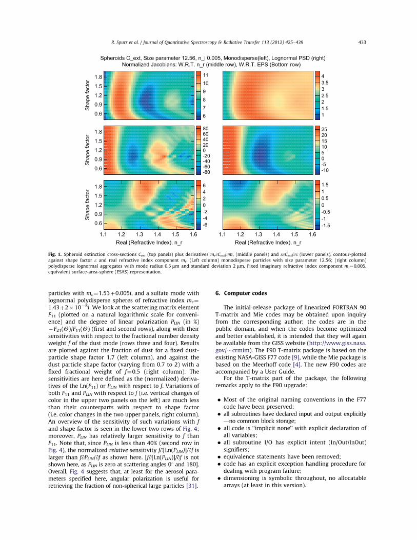
In Fig. 1, we look at the extinction cross-section Cextand its two normalized derivatives mr@Cext/@mr and e@Cext/@e for oblate and prolate spheroid particles, with incidentlight at wavelength 0.55 mm and fixed imaginary refrac-tive index component mi¼0.005. Results are plotted fora range of values [0.4, 2.0] for the shape factor e, anda range [1.1, 1.6] for the real refractive index componentmr. Calculations were done using the equivalent surfacearea sphere (ESAS) representation. Left panels show resultsfor a monodisperse situation with particle size 1 mm (sizeparameter �12.56), with the right panels containingresults for a polydisperse aggregate characterized by alognormal PSD with mode radius 0.5 mm and standarddeviation 2 mm.

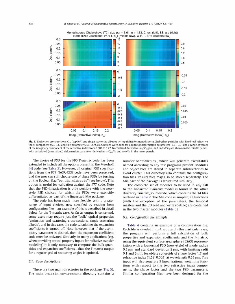
Focusing next on Chebyshev particles in Fig. 2, we lookat the extinction cross-section Cext and the single scatter-ing albedo o (top left and top right, respectively), andtheir normalized derivatives mi@Cext/@mi and mi@o/@mi

(middle row) with respect to the imaginary componentmi of the refractive index, and derivatives e@Cext/@eand e@o/@e (bottom row) with respect to the Chebyshevdeformation parameter. Incident light has wavelength0.95 mm and the real part of the refractive index compo-nent is fixed at mr¼1.33. Results are plotted for a range ofvalues [0.01, 0.3] for the deformation parameter e, and arange [0.002, 0.22] for the imaginary refractive indexcomponent mi. Calculations were done using the equiva-lent surface-area-sphere (ESAS) representation.

In Fig. 3, we return to oblate spheroids, looking thistime at angular distributions. Results are shown formonodisperse spheroids with shape factor e¼1.7 andrefractive index 1.42þ0.008i, at wavelength 0.443 mm.We look at the normalized scattering matrix elementF11(Y) and the corresponding degree of linear polariza-tion (in %) �F21(Y)/F11(Y) (top left and top right, respec-tively), along with their three derivatives e@/@e, mr@/@mr

and miq/qmi (rows 2 to 4, respectively). Results are plottedagainst scattering angle Y from 0 to 1801, and for a range[0, 20] for the particle size parameter. Calculations areagain done using the ESAS representation. The plot for�F21(Y)/F11(Y) (top right) is closely similar to one of thegraphs in Plate 2.1 of [5]. It can be seen that polarizationat backscattering angles has large sensitivity to changes ofshape factor; this offers the promise for retrieval ofparticle shape from multi-angle polarization measure-ments. The sensitivity drops significantly at scatteringangle close to 1801 for particles with size parameters lessthan 5; this is also the condition for low polarization.

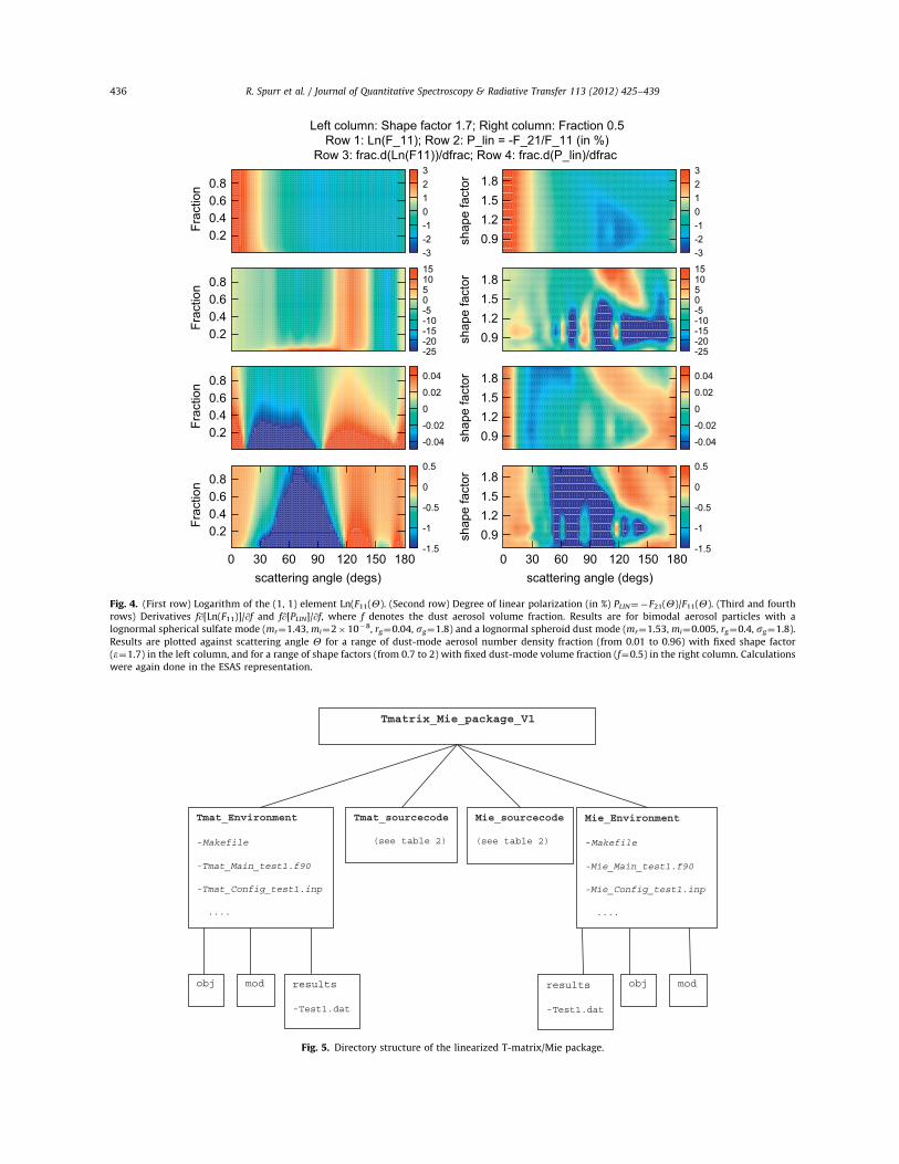
In Fig. 4, we look at a bimodal aggregate, comprisinga dust mode with lognormal polydisperse spheroidal


particles with mc¼1.53þ0.005i, and a sulfate mode withlognormal polydisperse spheres of refractive index mc¼1.43þ2�10�8i. We look at the scattering matrix elementF11 (plotted on a natural logarithmic scale for conveni-ence) and the degree of linear polarization PLIN (in %)�F21(Y)/F11(Y) (first and second rows), along with theirsensitivities with respect to the fractional number densityweight f of the dust mode (rows three and four). Resultsare plotted against the fraction of dust for a fixed dust-particle shape factor 1.7 (left column), and against thedust particle shape factor (varying from 0.7 to 2) with afixed fractional weight of f¼0.5 (right column). Thesensitivities are here defined as the (normalized) deriva-tives of the Ln(F11) or PLIN with respect to f. Variations ofboth F11 and PLIN with respect to f (i.e. vertical changes ofcolor in the upper two panels on the left) are much lessthan their counterparts with respect to shape factor(i.e. color changes in the two upper panels, right column).An overview of the sensitivity of such variations with f

and shape factor is seen in the lower two rows of Fig. 4;moreover, PLIN has relatively larger sensitivity to f thanF11. Note that, since PLIN is less than 40% (second row inFig. 4), the normalized relative sensitivity f@[Ln(PLIN)]/@f islarger than f@PLIN/@f as shown here. [f@[Ln(PLIN)]/qf is notshown here, as PLIN is zero at scattering angles 01 and 180].Overall, Fig. 4 suggests that, at least for the aerosol para-meters specified here, angular polarization is useful forretrieving the fraction of non-spherical large particles [31].

6. Computer codes

The initial-release package of linearized FORTRAN 90T-matrix and Mie codes may be obtained upon inquiryfrom the corresponding author; the codes are in thepublic domain, and when the codes become optimizedand better established, it is intended that they will againbe available from the GISS website (http://www.giss.nasa.gov/�crmim). The F90 T-matrix package is based on theexisting NASA-GISS F77 code [9], while the Mie package isbased on the Meerhoff code [4]. The new F90 codes areaccompanied by a User Guide.

For the T-matrix part of the package, the followingremarks apply to the F90 upgrade:

Most of the original naming conventions in the F77code have been preserved;

all subroutines have declared input and output explicitly—no common block storage;

all code is ‘‘implicit none’’ with explicit declaration ofall variables;

all subroutine I/O has explicit intent (In/Out/InOut)signifiers;

equivalence statements have been removed; code has an explicit exception handling procedure for

dealing with program failure; dimensioning is symbolic throughout, no allocatable

arrays (at least in this version).

Spheroids C_ext, Size parameter 12.56, n_i 0.005, Monodisperse(left), Lognormal PSD (right)Normalized Jacobians: W.R.T. n_r (middle row), W.R.T. EPS (Bottom row)

0.6

0.9

1.2

1.5

1.8

Sha

pe fa

ctor

67891011

11.522.533.54

0.6

0.9

1.2

1.5

1.8

Sha

pe fa

ctor

-80-60-40-20020406080

-10-50510152025

1.1 1.2 1.3 1.4 1.5 1.6Real (Refractive Index), n_r

0.6

0.9

1.2

1.5

1.8

Sha

pe fa

ctor

-6-4-20246

1.1 1.2 1.3 1.4 1.5 1.6Real (Refractive Index), n_r

-1.5-1-0.500.511.5

Fig. 1. Spheroid extinction cross-sections Cext (top panels) plus derivatives mr@Cext/@mr (middle panels) and e@Cext/@e (lower panels), contour-plotted

against shape factor e and real refractive index component mr. (Left column) monodisperse particles with size parameter 12.56; (right column)

polydisperse lognormal aggregates with mode radius 0.5 mm and standard deviation 2 mm. Fixed imaginary refractive index component mi¼0.005,

equivalent surface-area-sphere (ESAS) representation.


The choice of PSD for the F90 T-matrix code has beenextended to include all the options present in the Meerhoff[4] code (see Table 5). However, all original PSD specifica-tions from the F77 NASA-GISS code have been preserved,and the user can still choose one of these PSDs by turningon the Boolean flag ‘‘Do_PSD_Oldstyle’’ (see below). Thisoption is useful for validation against the F77 code. Notethat the PSD-linearization is only possible with the new-style PSD choices, for which the PSDs were explicitlydifferentiated as part of the linearized Mie package.

The code has been made more flexible, with a greaterrange of input choices, now specified by reading fromconfiguration files—an example of this is described in detailbelow for the T-matrix case. As far as output is concerned,some users may require just the ‘‘bulk’’ optical properties(extinction and scattering cross-sections, single scatteringalbedo), and in this case, the code calculating the expansioncoefficients is turned off. Note however that if the asym-metry parameter is desired, then the expansion coefficientcode must be activated. Similarly, in many applications (e.g.when providing optical property inputs for radiative transfermodeling) it is only necessary to compute the bulk quan-tities and expansion coefficients—thus the F-matrix outputfor a regular grid of scattering angles is optional.

6.1. Code descriptions

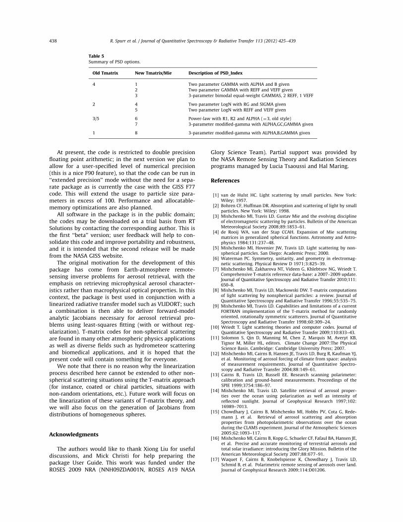
There are two main directories in the package (Fig. 5).The main Tmatrix_environment directory contains a

number of ‘‘makefiles’’, which will generate executablesnamed according to any test programs present. Modulesand object files are stored in separate subdirectories toavoid clutter. This directory also contains the configura-tion files. Results files may also be stored separately. TheMie part of the package is structured similarly.

The complete set of modules to be used in any callto the linearized T-matrix model is found in the otherdirectory Tmatrix_sourcecode, which contains the 14 filesoutlined in Table 2. The Mie code is simpler; all functions(with the exception of the parameters, the bimodalmasters and the I/O read and write routine) are containedin the two master modules (Table 3).

6.2. Configuration file example

Table 4 contains an example of a configuration file.Each file is divided into 4 groups. In this particular case,the program will perform a full calculation of bulkproperties and expansion coefficients and the F-matrix,using the equivalent surface area sphere (ESAS) represen-tation with a lognormal PSD (new-style) of mode radius0.5 mm and standard deviation 2 mm, with limiting radii0.1 and 5 mm, for oblate spheroids of shape factor 1.7 andrefractive index (1.53, 0.005) at wavelength 0.55 mm. Thisinput will also generate 5 linearizations: weighting func-tions with respect to the two refractive index compo-nents, the shape factor and the two PSD parameters.Similar configuration files have been designed for the

Monodisperse Chebyshevs (T2), size par = 6.61, n_r 1.33, C_ext (left), SS_alb (right) Normalized Jacobians: W.R.T. n_i (middle row), W.R.T. EPS (Bottom row)

0.05 0.1

0.15 0.2

0.25 0.3

Def

. par

am.

78910111213

0.5

0.6

0.7

0.8

0.9

0.05 0.1

0.15 0.2

0.25 0.3

Def

. par

am.

-2

-1.5

-1

-0.5

0

-0.2

-0.15

-0.1

-0.05

0.05 0.1 0.15 0.2Imag (Refractive Index), n_i

0.05 0.1

0.15 0.2

0.25 0.3

Def

. par

am.

-0.7-0.6-0.5-0.4-0.3-0.2-0.10

0.05 0.1 0.15 0.2Imag (Refractive Index), n_i

0

0.005

0.01

0.015

0.02

Fig. 2. Extinction cross-sections Cext (top left) and single scattering albedos o (top right) for monodisperse Chebyshev particles with fixed real refractive

index component mr¼1.33 and size parameter 6.61. ESAS calculations were done for a range of deformation parameters [0.01, 0.3] and a range of values

of the imaginary component of the refractive index from 0.002 to 0.22. Normalized derivatives mi@Cext/@mi and mi@o/@mi are shown in the middle panels,

with associated (normalized) deformation parameter derivatives e@Cext/@e and e@o/@e in the lower panels.


Mie code. In addition, there are configuration files forbimodal applications (requiring two sets of microphysicalvalues and PSD inputs).

6.3. Exception handling

Both the T-matrix and Mie codes have consistentexception handling procedures for dealing with inputchecking and execution failures. An overall Boolean flagis output for ‘‘success/failure’’, and there is also an integerstatus variable plus three character strings for outputmessages. Inputs are checked for consistency, and in thecase of input error, a message will be generated describ-ing the error, plus a second message outlining the actionrequired to correct the error along with 2 or 3 traces toestablish the location of the error. Dimensioning andconvergence issues are the main causes of T-matrixexecution failure, and the appropriate messages fromthe F77 code have been retained in the F90 package. Inboth codes, dimensioning checks will suggest new para-meters to use.

6.4. Particle-size distributions

Table 5 summarizes PSD options in the T-matrix andMie packages. For PSD_Index¼3 (Old-style power law)and FixR1R2¼T, then PSD_Par1 is an effective radius,PSD_Par2 an effective variance.

7. Concluding remarks

In this paper we have described a complete lineariza-tion of the T-matrix model as it applies to randomlyoriented axially symmetric particles. The linearity ofMaxwell’s equations and the intrinsic analytical natureof the T-matrix code allow us to carry out analyticdifferentiation of the entire T-matrix solution withrespect to any variables characterizing the particles inquestion. We distinguish two types of linearization: (1)with respect to single particle characteristics (real andimaginary components of the refractive index, particleshape or deformation factor), and (2) with respect toparticle size distribution parameters characterizing poly-disperse aggregations.

The NASA-GISS T-matrix code package has been trans-lated to Fortran 90, and additional code written to gen-erate the Type 1 and Type 2 optical property derivativesas noted in Section 2.1. The new code has been validatedagainst the old NASA-GISS FORTRAN 77 package, and alloptical property derivatives have been checked againstfinite-difference estimations. We have developed a sepa-rate linearization package for the Mie code, even thoughMie theory is a special case of the T-matrix formulation.The Type-1 Mie linearization applies only to derivativeswith respect to the refractive index components. Type-2linearizations apply equally to the Mie and T-matrixformulations.

Left Column : Ln(F_11) ; n_r.d(Ln(F11))/dn_r; n_i.d(Ln(F11))/dn_i; eps.d(Ln(F11))/depsRight Column: P_lin = -F_21/F_11 (in %); n_r.d(P_lin)/dn_r; n_i.d(P_lin)/dn_i; eps.d(P_lin)/deps

5

10

15

20

Siz

e pa

ram

eter

-3-2-1012345

5

10

15

20

Siz

e pa

ram

eter

-15-10-5051015

5

10

15

20

Siz

e pa

ram

eter

-0.4-0.200.20.4

0 45 90 135 180scattering angle (degs)

5

10

15

20

Siz

e pa

ram

eter

-4-20246810

-20-15-10-5 0 5 10 15 20

-100

-50

0

50

100

-4-2 0 2 4 6 8 10

0 45 90 135 180scattering angle (degs)

-100

-50

0

50

100

Fig. 3. Logarithm of the (1, 1) scattering matrix element Ln(F11(Y)) (top left panel); degree of linear polarization (in %) �F21(Y)/F11(Y) (top right panel).

The three derivatives mr@/@mr, mi@/@mi and e@/@e of these quantities are shown in rows 2, 3 and 4, respectively. Results are plotted for monodisperse

oblate spheroids (e¼1.7, mr¼1.42, mi¼0.008) against scattering angle Y for a range of particle size parameters as indicated. Calculations were again

done in the ESAS representation.


Row 1: Ln(F_11); Row 2: P_lin = -F_21/F_11 (in %)Row 3: frac.d(Ln(F11))/dfrac; Row 4: frac.d(P_lin)/dfrac

Left column: Shape factor 1.7; Right column: Fraction 0.5

0.2 0.4 0.6 0.8

Frac

tion

-3-2-10123

0.2 0.4 0.6 0.8

Frac

tion

-25-20-15-10-5051015

0.2 0.4 0.6 0.8

Frac

tion

-0.04

-0.02

0

0.02

0.04

0 30 60 90 120 150 180scattering angle (degs)

0.2 0.4 0.6 0.8

Frac

tion

-1.5

-1

-0.5

0

0.5

0.9 1.2 1.5 1.8

shap

e fa

ctor

-3-2-10123

0.9 1.2 1.5 1.8

shap

e fa

ctor

-25-20-15-10-5051015

0.9 1.2 1.5 1.8

shap

e fa

ctor

-0.04

-0.02

0

0.02

0.04

0 30 60 90 120 150 180scattering angle (degs)

0.9 1.2 1.5 1.8

shap

e fa

ctor

-1.5

-1

-0.5

0

0.5

Fig. 4. (First row) Logarithm of the (1, 1) element Ln(F11(Y). (Second row) Degree of linear polarization (in %) PLIN¼�F21(Y)/F11(Y). (Third and fourth

rows) Derivatives f@[Ln(F11)]/@f and f@[PLIN]/@f, where f denotes the dust aerosol volume fraction. Results are for bimodal aerosol particles with a

lognormal spherical sulfate mode (mr¼1.43, mi¼2�10�8, rg¼0.04, sg¼1.8) and a lognormal spheroid dust mode (mr¼1.53, mi¼0.005, rg¼0.4, sg¼1.8).

Results are plotted against scattering angle Y for a range of dust-mode aerosol number density fraction (from 0.01 to 0.96) with fixed shape factor

(e¼1.7) in the left column, and for a range of shape factors (from 0.7 to 2) with fixed dust-mode volume fraction (f¼0.5) in the right column. Calculations

were again done in the ESAS representation.

Fig. 5. Directory structure of the linearized T-matrix/Mie package.


Table 2Subdirectory ‘‘Tmatrix_sourcecode’’, F90 modules.

Module Purpose

tmat_parameters.f90 Dimensioning and type-kind parameters

tmat_distributions.f90 Computation of PSDs (old style and new style) and linearizations (new style only)

tmat_master.f90 Top-level module for computing optical property stuff, standard output only

tmat_master_PLUS.f90 Top-level module for computing optical property standard and linearized output

tmat_functions.f90 Work-horse routines for Bessel and other functions

tmat_functions_PLUS.f90 Work-horse routines for Bessel and other functions, and any linearizations thereof

tmat_makers.f90 Routines for creating Q, RgQ and T-matrix

tmat_makers_PLUS.f90 Routines for creating Q, RgQ and T-matrix, and all linearizations thereof

tmat_scattering.f90 Routines for calculating expansion coefficients and F-matrices

tmat_scattering_PLUS.f90 Routines for expansion coefficients and F-matrices, and all linearizations thereof

Utilities_LAPACK.f90 LAPACK routines (F90 syntactical translation of original F77 code)

Tmat_IO_readwrite.f90 Routines for reading configuration files and writing standard and extended outputs to files

Tmat_master_bimodal.f90 Bimodal wrapper, standard output

Tmat_master_bimodal_PLUS.f90 Bimodal wrapper, standard and linearized output

Table 3Subdirectory ‘‘Mie_sourcecode’’, F90 modules.

Module Purpose

Mie_parameters.f90 Mie dimensioning and type-kind parameters

Mie_distribution.f90 PSD distribution functions

Mie_main.f90 Mie module for computing optical properties, standard output only

Mie_main_PLUS.f90 Mie module for computing optical properties, standardþ linearized output

Mie_IO_readwrite.f90 Routines for reading configuration files and writing standard and extended outputs to files

Mie_master_bimodal.f90 Bimodal wrapper, standard output

Mie_master_bimodal_PLUS.f90 Bimodal wrapper, standard and linearized output

Table 4Configuration file example for the T-matrix model.

Value Name Description Remarks

*** First group (Boolean flags)

T Do_Expcoeffs Flag for expansion coefficient output New feature

T Do_Fmatrix Flag for optional F-matrix output New: Do_Expcoeffs must be set

F Do Monodisperse Flag for a monodisperse calculation New feature

T Do_EqSaSphere Flag for using equivalent surface area sphere (ESAS)

representation

Formerly a non-Boolean input

T Do_LinearRef Flag for linearizing w.r.t. real and imaginary parts of

refractive index

T Do_LinearEps Flag for linearizing w.r.t. shape parameter

T Do_LinearPSD Flag for linearizing w.r.t. PSD parameters Only works for the ‘‘New-style’’ PSD choices

F Do_psd_OldStyle Flag for using original PSD choices If set, use the NASA-GISS F77 original PSD choices

*** Second group (PSD control)

4 psd_index Particle size distribution (PSD) index See Table 5 for choices

0.5 psd_pars1 First PSD parameter See Table 5

2.0 psd_pars2 Second PSD parameter

0.0 psd_pars3 Third PSD parameter

1.0 Monoradius Size (mm) of equivalent-sphere particle Monodisperse only

F FixR1R2 Flag for fixing R1 & R2 internally Only if Do_psd_OldStyle not set

0.1 R1 Minimum radius (microns) Not needed if FixR1R2 is set

1.0 R2 Maximum radius (microns) Not needed if FixR1R2 is set

*** Third group (General control)

�1 np �1(spheroids), �2(cylinder), 40(Chebyshev) Same as GISS-F77 options

20 nkmax Number of PSD quadrature points Same name as in GISS-F77

91 npna Number of F-matrix outputs Same name as in GISS-F77

2 ndgs Number of ESAS division points Same name as in GISS-F77

2.0 eps Aspect ratio, deformation parameter , etc. Shape parameter

0.001 accuracy Accuracy for convergence As in GISS-F77, formerly DELT

*** Fourth group (optical inputs)

0.5 lambda Wavelength Always micrometers

1.53 n_real Real part of refractive index

0.008 n_imag Imaginary part of refractive index


At present, the code is restricted to double precisionfloating point arithmetic; in the next version we plan toallow for a user-specified level of numerical precision(this is a nice F90 feature), so that the code can be run in‘‘extended precision’’ mode without the need for a sepa-rate package as is currently the case with the GISS F77code. This will extend the usage to particle size para-meters in excess of 100. Performance and allocatable-memory optimizations are also planned.

All software in the package is in the public domain;the codes may be downloaded on a trial basis from RTSolutions by contacting the corresponding author. This isthe first ‘‘beta’’ version; user feedback will help to con-solidate this code and improve portability and robustness,and it is intended that the second release will be madefrom the NASA GISS website.

The original motivation for the development of thispackage has come from Earth-atmosphere remote-sensing inverse problems for aerosol retrieval, with theemphasis on retrieving microphysical aerosol character-istics rather than macrophysical optical properties. In thiscontext, the package is best used in conjunction with alinearized radiative transfer model such as VLIDORT; sucha combination is then able to deliver forward-modelanalytic Jacobians necessary for aerosol retrieval pro-blems using least-squares fitting (with or without reg-ularization). T-matrix codes for non-spherical scatteringare found in many other atmospheric physics applicationsas well as diverse fields such as hydrometeor scatteringand biomedical applications, and it is hoped that thepresent code will contain something for everyone.

We note that there is no reason why the linearizationprocess described here cannot be extended to other non-spherical scattering situations using the T-matrix approach(for instance, coated or chiral particles, situations withnon-random orientations, etc.). Future work will focus onthe linearization of these variants of T-matrix theory, andwe will also focus on the generation of Jacobians fromdistributions of homogeneous spheres.

Acknowledgments

The authors would like to thank Xiong Liu for usefuldiscussions, and Mick Christi for help preparing thepackage User Guide. This work was funded under theROSES 2009 NRA (NNH09ZDA001N, ROSES A19 NASA

Glory Science Team). Partial support was provided bythe NASA Remote Sensing Theory and Radiation Sciencesprograms managed by Lucia Tsaoussi and Hal Maring.

References

[1] van de Hulst HC. Light scattering by small particles. New York:Wiley; 1957.

[2] Bohren CF, Huffman DR. Absorption and scattering of light by smallparticles. New York: Wiley; 1998.

[3] Mishchenko MI, Travis LD. Gustav Mie and the evolving disciplineof electromagnetic scattering by particles. Bulletin of the AmericanMeteorological Society 2008;89:1853–61.

[4] de Rooij WA, van der Stap CCAH. Expansion of Mie scatteringmatrices in generalized spherical functions. Astronomy and Astro-physics 1984;131:237–48.

[5] Mishchenko MI, Hovenier JW, Travis LD. Light scattering by non-spherical particles. San Diego: Academic Press; 2000.

[6] Waterman PC. Symmetry, unitarity, and geometry in electromag-netic scattering. Physical Review D 1971;3:825–39.

[7] Mishchenko MI, Zakharova NT, Videen G, Khlebtsov NG, Wriedt T.Comprehensive T-matrix reference data-base: a 2007–2009 update.Journal of Quantitative Spectroscopy and Radiative Transfer 2010;111:650–8.

[8] Mishchenko MI, Travis LD, Mackowski DW. T-matrix computationsof light scattering by nonspherical particles: a review. Journal ofQuantitative Spectroscopy and Radiative Transfer 1996;55:535–75.

[9] Mishchenko MI, Travis LD. Capabilities and limitations of a currentFORTRAN implementation of the T-matrix method for randomlyoriented, rotationally symmetric scatterers. Journal of QuantitativeSpectroscopy and Radiative Transfer 1998;60:309–24.

[10] Wriedt T. Light scattering theories and computer codes. Journal ofQuantitative Spectroscopy and Radiative Transfer 2009;110:833–43.

[11] Solomon S, Qin D, Manning M, Chen Z, Marquis M, Averyt KB,Tignor M, Miller HL, editors. Climate Change 2007:The PhysicalScience Basis. Cambridge: Cambridge University Press; 2007.

[12] Mishchenko MI, Cairns B, Hansen JE, Travis LD, Burg R, Kaufman YJ,et al. Monitoring of aerosol forcing of climate from space: analysisof measurement requirements. Journal of Quantitative Spectro-scopy and Radiative Transfer 2004;88:149–61.

[13] Cairns B, Travis LD, Russell EE. Research scanning polarimeter:calibration and ground-based measurements. Proceedings of theSPIE 1999;3754:186–97.

[14] Mishchenko MI, Travis LD. Satellite retrieval of aerosol proper-ties over the ocean using polarization as well as intensity ofreflected sunlight. Journal of Geophysical Research 1997;102:16989–7013.

[15] Chowdhary J, Cairns B, Mishchenko MI, Hobbs PV, Cota G, Rede-mann J, et al. Retrieval of aerosol scattering and absorptionproperties from photopolarimetric observations over the oceanduring the CLAMS experiment. Journal of the Atmospheric Sciences2005;62:1093–117.

[16] Mishchenko MI, Cairns B, Kopp G, Schueler CF, Fafaul BA, Hansen JE,et al. Precise and accurate monitoring of terrestrial aerosols andtotal solar irradiance: introducing the Glory Mission. Bulletin of theAmerican Meteorological Society 2007;88:677–91.

[17] Waquet F, Cairns B, Knobelspiesse K, Chowdhary J, Travis LD,Schmid B, et al. Polarimetric remote sensing of aerosols over land.Journal of Geophysical Research 2009;114:D01206.

Table 5Summary of PSD options.

Old Tmatrix New Tmatrix/Mie Description of PSD_Index

4 1 Two parameter GAMMA with ALPHA and B given

2 Two parameter GAMMA with REFF and VEFF given

3 3-parameter bimodal equal-weight GAMMAS, 2 REFF, 1 VEFF

2 4 Two parameter LogN with RG and SIGMA given

5 Two parameter LogN with REFF and VEFF given

3/5 6 Power-law with R1, R2 and ALPHA (¼3, old style)

7 3-parameter modified-gamma with ALPHA,GC,GAMMA given

1 8 3-parameter modified-gamma with ALPHA,B,GAMMA given


[18] Hasekamp OP, Landgraf J. Linearization of vector radiative transferwith respect to aerosol properties and its use in satellite remotesensing. Journal of Geophysical Research 2005;110:D04203.

[19] Butz A, Hasekamp OP, Frankenberg C, Aben I. Retrievals of atmo-spheric CO2 from simulated space-borne measurements of back-scattered near-infrared sunlight: accounting for aerosol effects.Applied Optics 2009;48:332–6.

[20] Crisp D, Atlas RM, Breon F-M, Brown LR, Burrows JP, Ciais P, et al.The orbiting carbon observatory (OCO) mission. Advances in SpaceResearch 2004;34:700–9.

[21] Zeng J, Han Q, Wang J. High-spectral resolution simulation ofpolarization of skylight: sensitivity to aerosol vertical profile.Geophysical Research Letters 2008;35:L20801.

[22] Torres O, Bhartia PK, Herman JR, Ahmad Z, Gleason J. Derivation ofaerosol properties from satellite measurements of backscatteredultraviolet radiation, theoretical basis. Journal of GeophysicalResearch 1998;103:17099–110.

[23] Spurr R. LIDORT and VLIDORT: Linearized pseudo-spherical scalarand vector discrete ordinate radiative transfer models for use inremote sensing retrieval problems. In: Kokhanovsky A, editor. Lightscattering reviews, vol. 3. Berlin: Springer; 2008 p. 229–75.

[24] Mishchenko MI, et al. Aerosol retrievals from AVHRR radiances:effects of particle nonsphericity and absorption and an updatedlong-term global climatology of aerosol properties. Journal of

Quantitative Spectroscopy and Radiative Transfer 2003;79/80:953–72.

[25] Wang J, Liu X, Christopher SA, Reid JS, Reid E, Maring HB. Theeffects of non-sphericity on geostationary satellite retrievals of dustaerosols. Geophysical Research Letters 2003;30:2293.

[26] Grainger RG, Lucas J, Thomas GE, Ewan G. The calculation of Miederivatives. Applied Optics 2004;43:5386–93.

[27] Mishchenko MI, Travis LD, Lacis AA. Scattering, absorption, andemission of light by small particles. Cambridge: Cambridge Uni-versity Press; 2002 Available from /http://www.giss.nasa.gov/staff/mmishchenko/books.htmlS.

[28] Mishchenko MI. Multiple scattering, radiative transfer, and weaklocalization in discrete random media: unified microphysicalapproach. Reviews of Geophysics 2008;46:RG2003.

[29] Wiscombe WJ, Mugnai A. Scattering from nonspherical Chebyshevparticles. 2: means of angular scattering patterns. Applied Optics1988;27:2405–21.

[30] Tsang L, Kong JA, Shin RT. Theory of microwave remote sensing.New York: Wiley; 1985.

[31] Dubovik O, Herman M, Holdak A, Lapyonok T, Tanre D, Deuze JL,et al. Statistically optimized inversion algorithm for enhancedretrieval of aerosol properties from spectral multi-angle polari-metric satellite observations. Atmospheric Measurement Techni-ques 2011;4:957–1018.


Linearized T-matrix and Mie scattering computations … · Linearized T-matrix and Mie scattering...

Documents

Transcript of Linearized T-matrix and Mie scattering computations … · Linearized T-matrix and Mie scattering...