LINEARIZATION AND HEALTH ESTIMATION OF A TURBOFAN … · health parameter estimation of turbofan...
122
i LINEARIZATION AND HEALTH ESTIMATION OF A TURBOFAN ENGINE BHARATH REDDY ENDURTHI Bachelor of Engineering in Electronics and Instrumentation Engineering University of Madras, India June, 2001 Submitted in partial fulfillment of requirements for the degree MASTER OF SCIENCE IN ELECTRICAL ENGINEERING at the CLEVELAND STATE UNIVERSITY December, 2004
Transcript of LINEARIZATION AND HEALTH ESTIMATION OF A TURBOFAN … · health parameter estimation of turbofan...
i
LINEARIZATION AND HEALTH ESTIMATION OF A
TURBOFAN ENGINE
BHARATH REDDY ENDURTHI
Bachelor of Engineering in Electronics and Instrumentation Engineering
University of Madras, India
June, 2001
Submitted in partial fulfillment of requirements for the degree
MASTER OF SCIENCE IN ELECTRICAL ENGINEERING
at the
CLEVELAND STATE UNIVERSITY
December, 2004
ii
LINEARIZATION AND HEALTH ESTIMATION OF A
TURBOFAN ENGINE
BHARATH REDDY ENDURTHI
ABSTRACT
Jet engines are precision machines composed of many expensive parts characterized by a
large number of variables. An engine’s health deteriorates considerably over time.
Certain engine variables, known as health parameters, have a major effect on its health.
Monitoring and evaluating these health parameters help in developing predictive control
techniques and maintenance, thereby increasing the performance, life, reliability, and
safety of the engine. The main aim of this research is to estimate the health parameter
deterioration of a turbofan aircraft engine over a period of time. It is impossible to
directly measure the health parameters. We therefore estimate the health parameters using
an estimation technique based on the available measurements. The Kalman filter has been
shown to be an optimal estimator for linear systems. So the nonlinear engine model is
linearized with respect to three different sets of parameters (states, controls, and health
parameters) using three different linearization methods. This gives us 27 different
possible linear models for one nonlinear engine model. The different linearization
methods that will be discussed are the Matlab method, the perturbation method, and the
steady state error reduction method. Kalman filtering results are investigated for all 27
different linear models at two different operating conditions for the turbofan engine. A
graphical user interface is also developed to make the turbofan health estimation problem
more user friendly. The implementation of the unscented Kalman filter, a new nonlinear
estimation technique, is also discussed.

iii
ACKNOWLEDGEMENT
I would like to express my sincere indebtness and gratitude to my thesis advisor
Dr. Dan Simon, for the ingenious commitment, encouragement and highly valuable
advice he provided me over the entire course of this thesis. I would like to thank Sanjay
Garg and Donald Simon at the NASA Glenn Research Center, and the NASA Aviation
Safety Program, for generously providing funding for this work.
I would also like to thank my committee members Dr. Zhiqiang Gao and Dr. Sridhar
Ungarala for their support and advice.
I wish to thank my lab mates at the Embedded Control Systems Research Laboratory for
their encouragement and intellectual input during the entire course of this thesis without which
this work wouldn’t have been possible.
Finally, I wish to thank my roommates and all my friends who have always been a
constant source of inspiration to me.

iv
To my parents Smt. & Sri. E. Vijaya Reddy
v
TABLE OF CONTENTS
PAGE
LIST OF FIGURES…………………………………………………………………ix
LIST OF TABLES…………………………………………………………………..xi
CHAPTER I – INTRODUCTION………………………………………………..1
CHAPTER II – THE TURBOFAN ENGINE…………………………………..4
2.1 Jet propulsion theory…………………………………………………...5
2.2 Gas turbine engine (Turbojet)……………………………………….…7
2.2.1 Components of the jet engine………………………………..8
2.2.2 Types of jet engines…………………………………………10
2.2.3 Jet engines with afterburners……………………………….13
2.3 Engine performance…………………………………………………...14
2.3.1 Engine rating………………………………………………..14
2.3.2 Engine maintenance………………………………………...15
2.3.3 Engine performance deterioration………………………….15
2.4 Turbofan engine used in this research (MAPSS)……………………..16
2.5 Engine’s state space model…………………………………………....22
CHAPTER III – LINEAR STATE ESTIMATION……………………………25
3.1 Different estimation techniques………………………………………..26
vi
3.1.1 Least squares estimation…………………………………….26
3.1.2 Weighted least squares estimation…………………………...28
3.1.3 Bayesian estimation…………………………………………..29
3.1.4 Recursive least squares estimation…………………………...30
3.2 State estimation in a linear system……………………………………...35
3.3 Discrete time Kalman filter……………………………………………..37
CHAPTER IV – LINEARIZED KALMAN FILTER…………………………...43
4.1 Nonlinear estimation…………………………………………………….44
4.1.1 Linearized Kalman filter……………………………………....44
4.1.2 Extended Kalman filter………………………………………..47
4.2 Linearization…………………………………………………………….49
4.2.1 Matlab linearization…………………………………………...50
4.2.2 Perturbation linearization………………………………….….51
4.2.2a Linearization with respect to states…………………..51
4.2.2b Linearization with respect to control inputs.................52
4.2.3 Steady state error reduction method…………………………...53
4.2.3a Linearization with respect to states……………….…..53
4.2.3b Linearization with respect to controls………………...54
4.3 Linearization of the MAPSS turbofan engine model………………….....55
4.4 Discretization of the MAPSS linear model……………………………....56
4.5 Discrete Linearized Kalman filter…………………………………….….58
4.6 Health estimation graphical user interface…………………………….....60
vii
CHAPTER V – SIMULATION RESULTS………………………………………62
5. 1 Linearization of the MAPSS turbofan engine model…………………...63
5. 2 Health parameter estimation results…………………………………….70
5.2.1 Unconstrained Kalman filter estimates……………………….72
5.2.2 Constrained Kalman filter estimates………………………….75
CHAPTER VI – UNSCENTED KALMAN FILTER……………………………82
6.1 Unscented transformation………………………………………………..84
6.2 Unscented Kalman filter…………………………………………………87
6.2.1 Algorithm for additive noise…………………………………...89
6.2.2 Algorithm for non-additive noise………………………………92
6.3 Sigma point selection analysis…………………………………………...93
6.3.1 Algorithm for minimal skew simplex sigma point set………….95
6.3.2 Algorithm for spherical simplex sigma point set………………97
6.4 Inverted pendulum application…………………………………………..98
6.5 Simulation results……………………………………………………….101
CHAPTER VII – CONCLUSIONS AND FUTURE WORK…………………...104
7.1 Conclusions……………………………………………………………...104
7.2 Future work……………………………………………………………...106

viii
BIBLIOGRAPHY…………………………………………………………………108
ix
LIST OF FIGURES
FIGURE ……………………………………………………………………………PAGE
2.1 Inflated balloon………………………………………………………………………5
2.2 Inflated balloon with stem released……………………………………………….....5
2.3 Heron’s aeolipile………………………………………………………………….…6
2.4 Turbojet…………………………………………………………………….............10
2.5 Turboprop/ Turboshaft……………………………………………………………..11
2.6 Turbofan…………………………………………………………………………....12
2.7 Schematic of turbofan engine model……………………………………….............17
2.8 MAPSS block diagram (Module Interaction)………………………………….…...18
2.9 Component level model with engine components………………………….............20
2.10 MAPSS graphical user interface…………………………………………….…….21
3.1 Mean and covariance propagation…………………………………………….……40
4.1 Health estimation graphical user interface…………………………………….........61
5.1 RMS errors of 27 linear models……………………………………………….........66
5.2 Linear vs Nonlinear simulations…………………………………………………....68
5.3a Unconstrained RMS health parameters degradation estimation errors for 1st
operating condition……………………………………………………………………...74
5.3b Constrained RMS health parameters degradation estimation errors for 1st operating
condition………………………………………………………………………………...76
5.4a Unconstrained health parameter degradation estimates……………………….…...79
5.4b Constrained health parameter degradation estimates………………………….…...80

x
5.5a Unconstrained RMS health parameters degradation estimation errors for 2nd
operating condition……………………………………………………………………..81
5.5b Constrained RMS health parameters degradation estimation errors for 2nd operating
condition ……………………………………………………………………………….81
6.1 Principle of Unscented transformation…………………………………………..…87
6.2 Mean and covariance propagation in three different transformations……………...88
6.3 Inverted pendulum…………………………………………………………….........98
6.4a Estimation of position and velocity of the cart……………………………….......102
6.4b Estimation of angle and angular velocity of the pendulum………………………103

xi
LIST OF TABLES
TABLE…… ………………………………………………………………………..PAGE
I – Best RMS errors averaged over the entire simulation time………………………….65
II – Best RMS errors at the final time……………………………………………….......66
III – Linear models performance…………………………………………………….......69
IV – RMS health parameter estimation errors for the unconstrained Kalman filter
for 27 linear models….…………………………………………………………………..73
V – RMS health parameter estimation errors for the constrained Kalman Filter
for 27 linear models………………………………………………………………….......77

1
CHAPTER I
INTRODUCTION
Jet engine components are subject to degradation over their lifetime of use [1]. This
degradation affects the fuel economy and component life consumption of the turbine.
Performance data is collected periodically to evaluate (estimate) the health of the engine.
This evaluation (estimation) is then used to decide maintenance schedules. This offers the
benefits of improved safety and reduced operating costs. The data used for the health
evaluation is collected during the flight and analyzed post flight for maintenance
schedules. Various algorithms have been proposed to estimate the health parameters of a
jet engine such as weighted least squares [2], expert systems [3], neural networks [4],
Kalman filters [4] and genetic algorithms [5]. The research work presented here deals
with the application of Kalman filters for health parameter estimation.
The main aim of this thesis is to investigate various linearization techniques that
can be implemented to linearize the highly nonlinear turbofan engine model and then to
estimate its health parameters. Different estimation techniques like linearized Kalman

2
filter and unscented Kalman filter are to be implemented to estimate the engine health
parameters. Once the linear models are validated, their effects on the engine health
parameter estimates are checked. A graphical user interface for the implementation for
health parameter estimation of turbofan engine has to be developed. The implementation
of unscented Kalman filter, a new nonlinear estimation technique, for the turbofan engine
health parameter estimation is also discussed.
A turbofan engine model can be obtained from the basic knowledge of physics of
a turbofan. Chapter II discusses the working principle of a turbofan engine and also
describes the different kinds of turbofan engines. MAPSS (modular aero propulsion
system simulation) is the engine model used in this research. MAPSS is a prototype
(dynamic model) of a high pressure ratio, dual spool, low bypass military type turbofan
engine [6].
State estimation plays an important role in the field of control engineering.
Dynamic measurements from the system are considered while estimating the states of the
corresponding system. The basic estimation techniques implemented for the linear
systems are described in Chapter III. The Kalman filter has been applied in areas as
diverse as aerospace, marine navigation, nuclear power plant instrumentation,
demographic modeling, manufacturing, and many others. This filter, also considered to
be the optimal state estimator, is also discussed.
3
As the turbofan engine is highly nonlinear, linear estimation cannot be directly
implemented. Hence, nonlinear estimation techniques which are derived from the linear
state estimation are also discussed. The linearized Kalman filter, considered to be one of
the efficient nonlinear estimation techniques, is derived in Chapter IV. This nonlinear
estimation technique works on the linearized model of the nonlinear model. Hence the
linearization process and different kinds of linearization techniques are also discussed in
Chapter IV.
The implementation of the linearized Kalman filter to the turbofan engine is
discussed is Chapter VI. Various linear models of the MAPSS model are obtained and
their behavior is compared with the nonlinear MAPSS model. The results of the
implementation of the linearized Kalman filter with all of the linear models are shown.
Lots of research is being carried out in nonlinear estimation. The unscented
Kalman filter, a new estimation technique, is one result of that research [7]. The
unscented Kalman filter is derived to overcome the difficulties faced in the
implementation of the extended or linearized Kalman filter. Chapter VI discusses the
unscented Kalman filter and its application to a small state problem. The implementation
of the unscented Kalman filter for the turbofan model is discussed in Chapter VII.
4
CHAPTER II
THE TURBOFAN ENGINE
One should be able to understand the basic theories and terms of turbofan engines while
working with them. The turbofan engine works on jet propulsion theory. Propulsion is the
net force that results from unbalanced forces. These unbalanced forces are the result of
implementation of Newton’s laws of motion to certain objects. Gas (air) under pressure in
a sealed container exerts equal pressure on all surfaces of the container, therefore, all the
forces are balanced and there are no forces to make the container move. If there is a hole
in the container, gas (air) cannot push against that hole and thus the gas escapes. While
the air is escaping, the side of the container opposite to the hole has more pressure than
side with the hole. Therefore, the net pressures are not balanced and there is a net force
available to move the container. This principle is better explained with an inflated balloon
(container). A brief introduction of the jet propulsion theory is given in Section 2.1. The
working principle of gas turbine engine and different types of gas turbine engines are
discussed in Section 2.2. Section 2.3 explains the engine performance, and is immediately
followed by Section 2.4 which describes the turbofan engine used in this research. Finally
Section 2.5 describes the modeling of the turbofan engine.
5
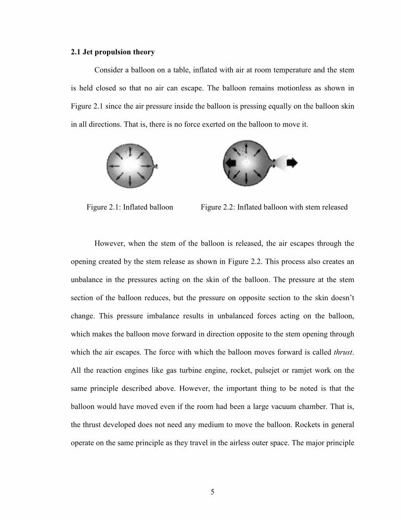
2.1 Jet propulsion theory
Consider a balloon on a table, inflated with air at room temperature and the stem
is held closed so that no air can escape. The balloon remains motionless as shown in
Figure 2.1 since the air pressure inside the balloon is pressing equally on the balloon skin
in all directions. That is, there is no force exerted on the balloon to move it.
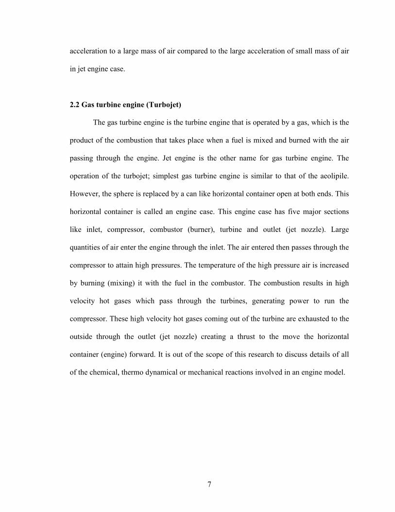
Figure 2.1: Inflated balloon Figure 2.2: Inflated balloon with stem released
However, when the stem of the balloon is released, the air escapes through the
opening created by the stem release as shown in Figure 2.2. This process also creates an
unbalance in the pressures acting on the skin of the balloon. The pressure at the stem
section of the balloon reduces, but the pressure on opposite section to the skin doesn’t
change. This pressure imbalance results in unbalanced forces acting on the balloon,
which makes the balloon move forward in direction opposite to the stem opening through
which the air escapes. The force with which the balloon moves forward is called thrust.
All the reaction engines like gas turbine engine, rocket, pulsejet or ramjet work on the
same principle described above. However, the important thing to be noted is that the
balloon would have moved even if the room had been a large vacuum chamber. That is,
the thrust developed does not need any medium to move the balloon. Rockets in general
operate on the same principle as they travel in the airless outer space. The major principle

6
being the conversion of the energy of expanding air (gases) in to mechanical force
(thrust).
Heron of Alexandria (Hero) built the first reaction engine somewhere around 250
B.C. Heron devised a machine called aeolipile shown in Figure 2.3, which was a closed
vessel in the shape of a sphere with two bent tubes mounted on its surface opposite to
each other. Steam at very high pressure was continuously introduced in to the sphere. The
high pressure steam escaped through the two tubes resulting in a force rotating the sphere
about an axis. The principle behind this phenomenon was not fully understood until 1690
A.D. when Sir Isaac Newton in England formulated the principle of Hero's jet propulsion
"aeolipile" in scientific terms. His Third Law of Motion stated: "Every action produces a
reaction ... equal in force and opposite in direction."
Figure 2.3: Heron’s aeolipile
All the jet engines designed operate on the same principle. Although there are
piston engines which work similar to the jet engines, they are rarely used in the aircrafts.
Both the engines convert the energy of the expanding gases in to mechanical force
(thrust). The major drawback in the piston engines is that they impart relatively small
7
acceleration to a large mass of air compared to the large acceleration of small mass of air
in jet engine case.
2.2 Gas turbine engine (Turbojet)
The gas turbine engine is the turbine engine that is operated by a gas, which is the
product of the combustion that takes place when a fuel is mixed and burned with the air
passing through the engine. Jet engine is the other name for gas turbine engine. The
operation of the turbojet; simplest gas turbine engine is similar to that of the aeolipile.
However, the sphere is replaced by a can like horizontal container open at both ends. This
horizontal container is called an engine case. This engine case has five major sections
like inlet, compressor, combustor (burner), turbine and outlet (jet nozzle). Large
quantities of air enter the engine through the inlet. The air entered then passes through the
compressor to attain high pressures. The temperature of the high pressure air is increased
by burning (mixing) it with the fuel in the combustor. The combustion results in high
velocity hot gases which pass through the turbines, generating power to run the
compressor. These high velocity hot gases coming out of the turbine are exhausted to the
outside through the outlet (jet nozzle) creating a thrust to the move the horizontal
container (engine) forward. It is out of the scope of this research to discuss details of all
of the chemical, thermo dynamical or mechanical reactions involved in an engine model.
8
2.2.1 Components of the jet engine
The working principle of a turbofan described above would be more clearly
understood by studying its main parts. There are five main parts of a turbofan or any gas
turbine engine, which play an important role in the engine’s operation.
a) Inlet
Air enters in to the engine through the inlet. The main task of the inlet is to
straighten out the flow, making it uniform and without much turbulence. This is
important because compressors and fans need to be fed distortion-free air. Inlet is
positioned just before the compressor. There are different types of inlets based on the
speed of the aircraft like subsonic inlets, supersonic inlets and hypersonic inlets.
b) Compressor
A compressor is used to increase the pressure of the air entering through the inlet.
The air is forced through several rows of both spinning and stationary blades. As the air
passes each row, the available space is greatly reduced, and so the air that exits this phase
is thirty or forty times higher in pressure than it was outside the engine. The temperature
of the air also gets increased because of the increase in pressure. Axial flow compressor
and centrifugal compressor are the two main types of computers used in turbofan engines.
The compressor is mounted in front of the combustor.
c) Burner (combustor)
The burner is the component in which the actual reaction (combustion) takes
place. The high pressure hot air coming out of the compressor is combined with the fuel
and burned for combustion. The combustion results in very high temperature gases with
high velocities. These high temperature exhaust gases are used to drive the turbine.
9
Burners, placed just after the compressors, are made from materials that can withstand
the high temperatures of combustion. Annular, can, can-annular burners are the three
different types of burners mostly used.
d) Turbine
The turbine is located next to the burner. The power used to drive the compressors
is obtained from turbines. The turbine extracts the energy of the high temperature gas
flow coming out of the burner by rotating the blades. This energy is transferred to the
compressors by connecting shafts. The air leaving the turbine has low temperature and
pressure when compared with the air coming out of the burner because of the energy
extraction. Turbine blades must be made of special materials that can withstand the heat,
or they must be actively cooled. There can be multiple turbine stages for driving different
parts of the engine independently like compressor, fan (turbofan) or propeller
(turboprop).
e) Nozzle (exhaust)
A nozzle is a specially shaped tube through which the hot gases flow. The actual
thrust required to move the engine forward is produced in this nozzle which is positioned
after the turbine stage in the engine. The thrust is developed by conducting the hot
exhaust gases through this nozzle to the free stream of outside air. Like the air leaving a
balloon described in the Section 2.1, the speed and flow rate of the air leaving the nozzle
provides the airplane with thrust. Both the temperature and pressure of the air or rather
hot gases is reduced very much while passing through the nozzle. The inside walls of the
nozzle are shaped so that the exhaust gases continue to increase their velocity as they
10
travel out of the engine. Based on the geometry of the nozzle, it can be categorized under
co-annular, convergent or convergent-divergent (CD) nozzle.
2.2.2 Types of jet engines
There are many different types of jet engines for aircraft like turbojet, turbofan,
turboprop, and turboshaft engines. These, in turn, can be subdivided based on their design
and internal arrangement of their components like single compressor engine, dual
compressor (twin spool) engines, high bypass ratio engines, and low bypass ratio engines.
All of the gas turbine engines like turbofans, turboprops and turboshaft engines work on
the same principle as the above described turbojet. As the turbofan being the engine used
in this research, a detailed explanation of the gas turbine engine (turbofan) operation is
presented in the sections to be followed.
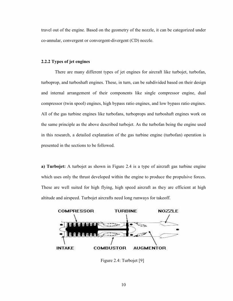
a) Turbojet: A turbojet as shown in Figure 2.4 is a type of aircraft gas turbine engine
which uses only the thrust developed within the engine to produce the propulsive forces.
These are well suited for high flying, high speed aircraft as they are efficient at high
altitude and airspeed. Turbojet aircrafts need long runways for takeoff.
Figure 2.4: Turbojet [9]

11
b) Turboprop: A turboprop is a turbojet engine with an additional turbine augmented to
it to drive a propeller (through a speed reducing gear system). Figure 2.5 shows the
schematic of a Turboprop. These engines are also called as propjets. The additional
turbine placed in the path of the exhaust gases is called the free turbine. This free turbine
is mounted on the shaft that drives the propeller.
Figure 2.5: Turboprop/ Turboshaft [9]
c) Turboshaft: The turboprop engine in which the shaft of the free turbine is used to
drive something other than the propeller is called the turboshaft. The other things that can
be driven by the free turbine shaft are rotor of a helicopter, boats, ships, trains and
automobiles. The shaft turbine engine is the other name for turboshaft engine.
Both the turboprop and turboshaft engines are more complicated and heavier than
the turbojet engine. They produce more thrust at low subsonic speeds. Their propulsive
efficiency (output divided by input) decreases as the speed increases, where as it
increases in the turbojet case.
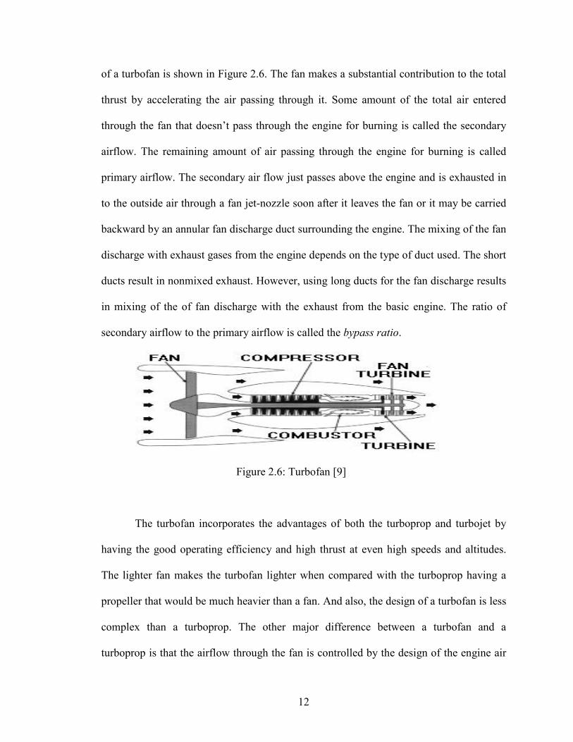
d) Turbofan: A turbofan is similar to the turboprop with the gear driven propeller
replaced with an axial flow fan with rotating blades and stationary vanes. The schematic
12
of a turbofan is shown in Figure 2.6. The fan makes a substantial contribution to the total
thrust by accelerating the air passing through it. Some amount of the total air entered
through the fan that doesn’t pass through the engine for burning is called the secondary
airflow. The remaining amount of air passing through the engine for burning is called
primary airflow. The secondary air flow just passes above the engine and is exhausted in
to the outside air through a fan jet-nozzle soon after it leaves the fan or it may be carried
backward by an annular fan discharge duct surrounding the engine. The mixing of the fan
discharge with exhaust gases from the engine depends on the type of duct used. The short
ducts result in nonmixed exhaust. However, using long ducts for the fan discharge results
in mixing of the of fan discharge with the exhaust from the basic engine. The ratio of
secondary airflow to the primary airflow is called the bypass ratio.
Figure 2.6: Turbofan [9]
The turbofan incorporates the advantages of both the turboprop and turbojet by
having the good operating efficiency and high thrust at even high speeds and altitudes.
The lighter fan makes the turbofan lighter when compared with the turboprop having a
propeller that would be much heavier than a fan. And also, the design of a turbofan is less
complex than a turboprop. The other major difference between a turbofan and a
turboprop is that the airflow through the fan is controlled by the design of the engine air

13
inlet duct in such a manner that the velocity of the air through the fan blades is not greatly
affected by the speed of the aircraft. This is the reason for turbofan being more efficient
than turboprops at higher speeds.
The turbofan has the advantage of lower noise level for the engine exhaust, when
compared with the turbojet delivering same thrust as the turbofan. This lower noise level,
an important feature in all commercial airports, makes the turbofan better choice than
turbojet. For the above described advantages of the turbofans and many other
characteristics, they have become the most widely used power plants (engines) for all
conventional large aircrafts, both military and commercial.
The turbofan engines can be subdivided based on the type of fan discharge duct
used like long duct or short duct, the amount of bypass ratio like high bypass or low
bypass.
2.2.3 Jet engines with afterburners
The military aircrafts like fighter jets require extra busts of a speed during takeoff
and climb, or for an intercept mission. This extra speed is achieved by an afterburner
added to their engine. An additional thrust of 50 percent or more thrust can be achieved
with jet engine equipped with an afterburner. The afterburner is also called an augmentor
because it is nothing but a pipe attached to the rear of an engine instead of a tail pipe and
jet nozzle. Only 25 percent of the air entering the fan is passed through the basic engine
for combustion, the remaining 75 percent of the air flow is just passed above the engine.
14
Sometimes it is mixed with the exhaust gases at the jet nozzle as in long duct type jet
engines; however it can be used for combustion in the afterburner by injecting the fuel
through spray bars. This additional combustion of exhaust gases (mixed with secondary
air flow) results in higher velocities delivering additional thrust. The afterburners develop
additional thrust at the cost of additional fuel consumption, so the use of an afterburner is
profitable only in those aircrafts that may urgently require increased speed for short
periods of time or extra power for short takeoff with heavy loads without considering the
fuel consumption.
2.3 Engine performance
Apart from the above described components, a turbofan has many other important
components which make the engine perform efficiently. Engine has a lot of actuators,
sensors and other instruments mounted on each of its components. These instruments
measure some critical parameters of the engine that would reveal the engine performance.
2.3.1 Engine rating
Engine ratings for different flights of an aircraft describe the engine performance
over a period of time. The thrust, in pounds, which an engine is designed to develop for
takeoff, maximum continuous, maximum climb, and maximum cruise is called the engine
rating [8]. These ratings are also interpreted in terms of engine pressure ratio (EPR). EPR
can be maintained by the Engine’s throttle position which regulates the supply of fuel.
Engine ratings are different for military and commercial engines as they are used for
different operations. In military aircraft, the urgency of the mission frequently determines
15
how the engine will be operated. While in commercial or passenger aircraft, the time
between the engine overhaul schedules and maximum reliability are of concern, and more
conservative engine operation becomes the rule.
2.3.2 Engine maintenance
Jet engines are precision machines composed of many expensive parts. A
thorough understanding of the construction and operation of an engine and its
components is vital to good jet engine maintenance. The maintenance in jet engine is
divided in to two categories: a) preventive maintenance and b) corrective maintenance.
The routine inspection of the various engine components, assemblies, and systems come
under the preventive maintenance category. Corrective maintenance is the one in which
the malfunctions and damaged parts are fixed or replaced as they occur.
Even though the operation manual of the engine described by the manufacturer
gives the details of how often to perform maintenance schedules, the engine performance
over a period of time is considered for scheduling the above maintenances to enhance the
engine’s life. It is a well known fact that any machine’s performance degrades for the
period of time it works. A turbofan engine’s performance also deteriorates over time as it
is also a kind of machine.
2.3.3 Engine performance deterioration
As described in the previous section, the engine’s performance deterioration plays
an important role in the engine maintenance schedule. Engine performance deterioration

16
also reduces the fuel economy of the engine [10]. Just like the life of a living being is
affected by its health, the life of a turbofan is also affected by its performance over a
period. Engine’s performance is also referred by other terms like health or condition.
There are many parameters of the engine which would fully describe the engine’s health.
It would be impossible or rather difficult to consider all the parameters that would add to
the engine’s health. Hence, only a certain number of parameters are considered which
would have a major effect on the engine’s health. These parameters are called health
parameters. Different engines have different set of health parameters.
Engine condition monitoring devices are used to measure most of the health
parameters of the engine. However, some of the parameters cannot be measured because
of many difficulties like the problem of mounting the device in a particular position,
unavailability of devices for measuring certain parameters, getting inaccurate
measurements from the devices or due to the complex design of the turbofan engine.
Monitoring and evaluating these health parameters by some means would help in good
maintenance and also increase the life of engine. Engine health evaluation can also be
very helpful in some predictive control techniques.
2.4 Turbofan engine used in this research (MAPSS)
The engine that is being implemented in this research is a high pressure ratio, dual
spool, low bypass military type turbofan engine shown in Figure 2.7, with a digital
controller. This engine has all of the basic components as discussed previously in Section
2.2. MAPSS, a generic nonlinear, low frequency, transient, high performance model is
17
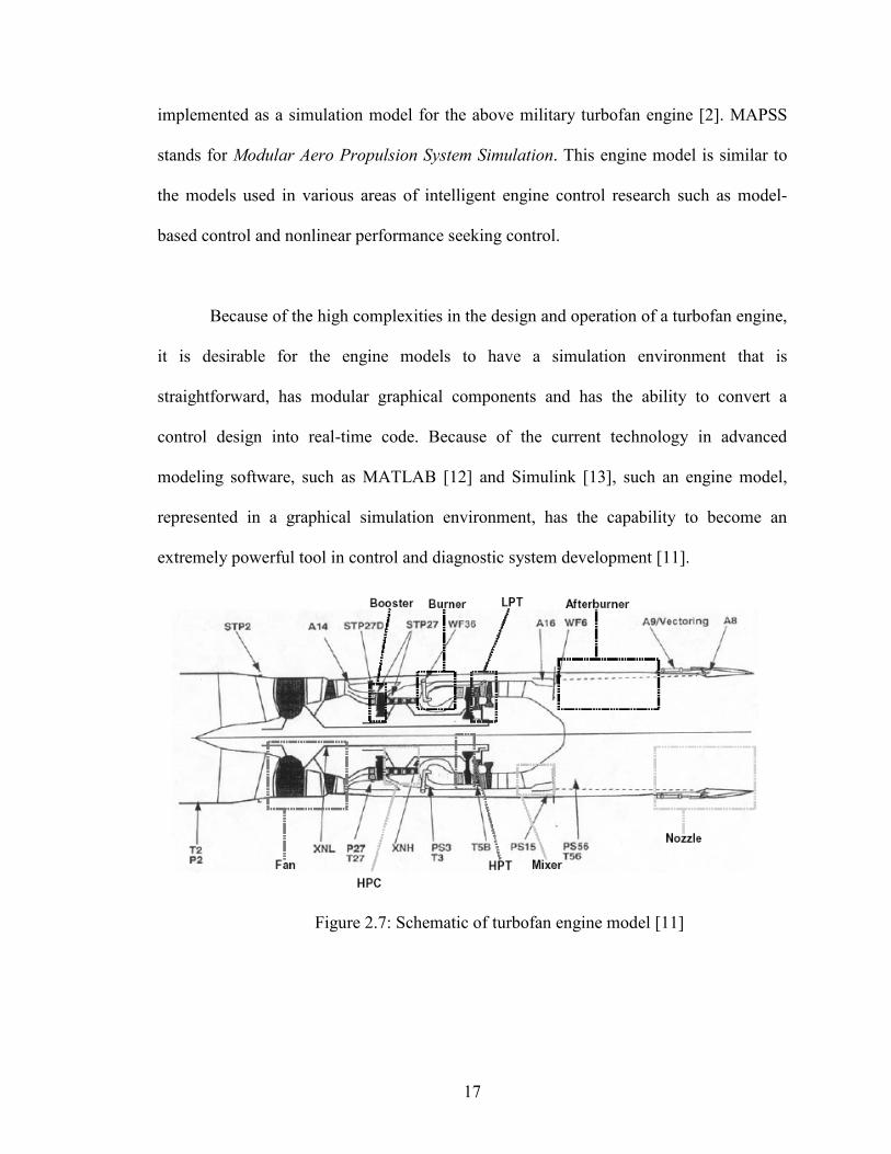
implemented as a simulation model for the above military turbofan engine [2]. MAPSS
stands for Modular Aero Propulsion System Simulation. This engine model is similar to
the models used in various areas of intelligent engine control research such as model-
based control and nonlinear performance seeking control.
Because of the high complexities in the design and operation of a turbofan engine,
it is desirable for the engine models to have a simulation environment that is
straightforward, has modular graphical components and has the ability to convert a
control design into real-time code. Because of the current technology in advanced
modeling software, such as MATLAB [12] and Simulink [13], such an engine model,
represented in a graphical simulation environment, has the capability to become an
extremely powerful tool in control and diagnostic system development [11].
Figure 2.7: Schematic of turbofan engine model [11]
18
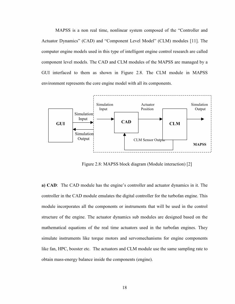
MAPSS is a non real time, nonlinear system composed of the “Controller and
Actuator Dynamics” (CAD) and “Component Level Model” (CLM) modules [11]. The
computer engine models used in this type of intelligent engine control research are called
component level models. The CAD and CLM modules of the MAPSS are managed by a
GUI interfaced to them as shown in Figure 2.8. The CLM module in MAPSS
environment represents the core engine model with all its components.
Input
Simulation
Input
Simulation
Output
Figure 2.8: MAPSS block diagram (Module interaction) [2]
a) CAD: The CAD module has the engine’s controller and actuator dynamics in it. The
controller in the CAD module emulates the digital controller for the turbofan engine. This
module incorporates all the components or instruments that will be used in the control
structure of the engine. The actuator dynamics sub modules are designed based on the
mathematical equations of the real time actuators used in the turbofan engines. They
simulate instruments like torque motors and servomechanisms for engine components
like fan, HPC, booster etc. The actuators and CLM module use the same sampling rate to
obtain mass-energy balance inside the components (engine).
Simulation Actuator Simulation
Input Position Output
CLM Sensor Output
MAPSS
GUI
CAD
CLM
19
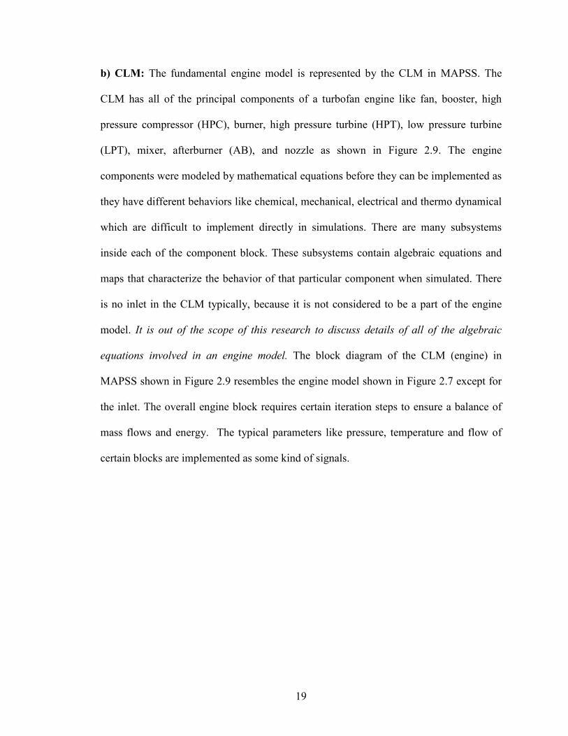
b) CLM: The fundamental engine model is represented by the CLM in MAPSS. The
CLM has all of the principal components of a turbofan engine like fan, booster, high
pressure compressor (HPC), burner, high pressure turbine (HPT), low pressure turbine
(LPT), mixer, afterburner (AB), and nozzle as shown in Figure 2.9. The engine
components were modeled by mathematical equations before they can be implemented as
they have different behaviors like chemical, mechanical, electrical and thermo dynamical
which are difficult to implement directly in simulations. There are many subsystems
inside each of the component block. These subsystems contain algebraic equations and
maps that characterize the behavior of that particular component when simulated. There
is no inlet in the CLM typically, because it is not considered to be a part of the engine
model. It is out of the scope of this research to discuss details of all of the algebraic
equations involved in an engine model. The block diagram of the CLM (engine) in
MAPSS shown in Figure 2.9 resembles the engine model shown in Figure 2.7 except for
the inlet. The overall engine block requires certain iteration steps to ensure a balance of
mass flows and energy. The typical parameters like pressure, temperature and flow of
certain blocks are implemented as some kind of signals.
20
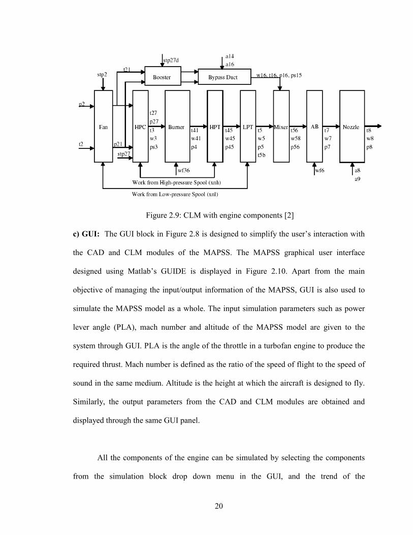
Figure 2.9: CLM with engine components [2]
c) GUI: The GUI block in Figure 2.8 is designed to simplify the user’s interaction with
the CAD and CLM modules of the MAPSS. The MAPSS graphical user interface
designed using Matlab’s GUIDE is displayed in Figure 2.10. Apart from the main
objective of managing the input/output information of the MAPSS, GUI is also used to
simulate the MAPSS model as a whole. The input simulation parameters such as power
lever angle (PLA), mach number and altitude of the MAPSS model are given to the
system through GUI. PLA is the angle of the throttle in a turbofan engine to produce the
required thrust. Mach number is defined as the ratio of the speed of flight to the speed of
sound in the same medium. Altitude is the height at which the aircraft is designed to fly.
Similarly, the output parameters from the CAD and CLM modules are obtained and
displayed through the same GUI panel.
All the components of the engine can be simulated by selecting the components
from the simulation block drop down menu in the GUI, and the trend of the
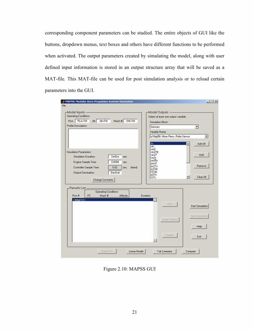
21
corresponding component parameters can be studied. The entire objects of GUI like the
buttons, dropdown menus, text boxes and others have different functions to be performed
when activated. The output parameters created by simulating the model, along with user
defined input information is stored in an output structure array that will be saved as a
MAT-file. This MAT-file can be used for post simulation analysis or to reload certain
parameters into the GUI.
Figure 2.10: MAPSS GUI
22
2.5 Engine’s state space model
Mathematical equations, typically differential or difference equations are used to
describe the behavior of processes and to predict their response to certain inputs [14].
These set of equations put in to a common framework is called as the state space model
of the system. This process of describing the systems by state space models is termed as
modeling. These models have many useful features like giving an intuitive understanding
of the behavior of many dynamical systems and can also be solved efficiently since they
are mathematical equations.
( , )x f x u=&
( , )y h x u= (2.1)
Any state space model can be represented with combinations of three parameters
of the system as shown in Equation 2.1. These three parameters namely states, inputs and
outputs describe the system’s behavior as a whole. The inputs and outputs constitute to be
the external variables, where as states form the internal variables of the system. The state
of a dynamic system is defined as the smallest set of variables such that the knowledge of
these variables together with the knowledge of inputs determines the behavior of system
at any time.
Similarly, the turbofan engine modeled as MAPSS has a set of states, control
inputs and outputs that describe the engine’s behavior. The three states of the MAPSS are
1) High pressure rotor speed (xnh)
2) Low pressure rotor speed (xnl)
3) Heat soak temperature (tmpc)
23
The three control inputs to the model are
1) Main burner fuel flow
2) Variable nozzle area
3) Rear BP door variable area
The eleven sensor outputs of the model are as follows
1) LPT exit pressure
2) LPT exit temperature
3) Percent low pressure spool rotor speed
4) HPC inlet temperature
5) HPC exit temperature
6) Bypass duct pressure
7) Fan exit pressure
8) Booster inlet pressure
9) HPC exit pressure
10) Core rotor speed
11) LPT blade temperature
Apart from the above mentioned parameters there are certain important
parameters called health parameters that describe the health of an engine. The importance
of these parameters was already discussed in Section 2.3. Estimating these health

24
parameters over a period of time is the objective of this research. The ten health
parameters of the MAPSS model are
1) Fan airflow
2) Fan efficiency
3) Booster tip airflow
4) Booster tip efficiency
5) Booster hub airflow
6) Booster hub efficiency
7) High pressure turbine airflow
8) High pressure turbine efficiency
9) Low pressure turbine airflow
10) Low pressure turbine efficiency
25
CHAPTER III
LINEAR STATE ESTIMATION
State feedback plays a major role in the control structure of any system. Stability and
other desired responses of the system depend on the state feedback given to the system.
In practice, the individual state variables of a dynamic system cannot be determined
exactly by direct measurements, such as the temperature in the core of a nuclear power
plant; instead, the measurements which are functions of state variables are used to
estimate the state variables indirectly. It should be noted that these measurements have
some random noise associated with them or system by itself might be corrupted with
some random noise.
To overcome such problems, estimators are designed based upon known
information regarding process (system dymanics) and the noise paramters, to provide a
good estimate of the states from the noisy mesurement data. Depending on the paramters
used with in the estimator, different terms are used to refer the estimation procedure.
Filtering refers to estimating the state vector at the current time, based upon all past
measurements. Prediction refers to estimating the state at a future time. Smoothing refers
26
to estimating the value of the state at some prior time, based on all measurements taken
up to the current time [15]. The difference between the estimator’s output and the true
state is termed as estimation error which is also used as the cost function for the
estimator. It is obvious to think that the estimation error has to be minimum for the state
estimates to be as close as possible to the true states. Thus, an estimator which provides
the estimates with optimum (minimum) estimation error is called an optimal state
estimator. Section 3.1 discusses different kinds of estimation techniques, and Section 3.2
describes state estimation in time varying systems. The classical Kalman filter equations
are derived in Section 3.3.
3.1 Different estimation techniques
Estimation techniques can be classified based on the criterion of their cost
function. For easy understanding of the reader, the estimation of a constant is considered
first before discussing the estimation of a time varying vector.
3.1.1 Least squares estimation
Suppose there are n measurements for a same scalar constant x, then intuitively
the average (mean) of the n measurements would result in estimate of x . This estimate is
optimal in the sense that it minimizes the sum of the squared errors (SSE) between the
measurements and the predicted measurements, and is a linear function of the
measurements [15].
27
Consider an n-dimensional constant vector x which is unknown, and a
measurement vector z related to the constant vector x obtained from k measurements. Let
e be the error in mesurements and H be the observation matrix of k × n dimension. Then
the relation between x and z is given by Equation 3.1 below,
z Hx e= + (3.1)
Now, if x̂ is the estimate of the true state x, then the error between true and
estimated state called the state residual ( xε ) is given by Equation 3.2a.
ˆx xxε = − (3.2a)
ˆz Hxzε = − (3.2b)
Similar to the state residual, the error in true measurement and estimated
measurements is called the measurement residual and is obtained as zε in
Equation 3.2b.
The cost function represented by J is defined as follows
1( )
2
TEJ z zε ε=
1(
2ˆ ˆ ˆ ˆ)T T T T T TJ E z z H z z H H Hx x x x= − − + (3.3)
Minimizing J with respect to x̂ would result in the best estimate x̂ for true state
x, i.e., partially differentiating J with respect to x̂ .
0x̂
J=
∂∂
results in
1ˆ ( )T Tx H H H z−= (3.4)
ˆ Lx H z=
28
where LH is the left pseudo inverse of H . This exists only when the number of known
variables (measurements) is greater than the number of unknowns (states).
3.1.2 Weighted least squares estimation
This kind of estimation is used when there is a weighting function on the errors
for different measurements. The weighting function was identical for all the
measurements in the previous section, where all measurements were obtained with error
statistics. Weighting functions are assigned to the error vectors when measurements were
obtained with different error statistics, i.e., when we have more confidence in some
measurements than others. The cost function for weighted least squares estimator can be
derived by incorporating this additional information about the errors weighting function.
Consider the same vector x as in Equation 3.1, with weighting functions for the
error vector as follows.
2 2
1 1
2 2
( )
( )k k
E e
E e
σ
σ
=
=
M (3.5)
The cost function J is defined to be the quadratic cost function of a normalized
measurement residual as in the following Equation 3.5 [16].
( )1 1
2E T TJ N Nz zε ε− −= (3.6)
where N is the k x k diagonal matrix defined as
1 0
0 k
N
σ
σ
=L
M O M
L
Minimizing the cost function J would result in the best estimate x̂ as
29
1 1 1ˆ ( )T Tx H S H H S z− − −= (3.7)
where TS N N≡
3.1.3 Bayesian estimation
Least squares estimation being a deterministic approach can only be used in the
case where there is no probabilistic description for either the unknown to be estimated or
the measurements considered. However, the maximum likelihood philosophy is used
when the x and z are assigned with some probability density functions. In this approach
the estimate x̂ will take that value which maximizes the probability of the measurements
z that actually occurred, taking into account known statistical properties of e [15].
Considering the same example as in Equation 3.1, the conditional probability
density function for z, conditioned on a given value for x, is just the density for e centered
around Hx. Considering e to be a zero mean, Gaussian distributed observation with
covariance matrix R, we get
1
1/ 2 1/ 2
1 1( | ) exp ( ) ( )
(2 ) | | 2
Tp z x z Hx R z HxRπ
− = − − − (3.8)
The objective of maximizing this probability of measurements is done by
minimizing the exponent in brackets. Minimizing this exponent is similar to minimizing
the cost function in Equation 3.6, with R replacing the TN N matrix, i.e., interpreting the
noise vector with its probabilistic covariance. Hence, the estimate would be the same
result as obtained in Equation 3.7, but with S replaced by R.
30
1 1 1ˆ ( )T Tx H R H H R z− − −= (3.9)
Bayesian estimation, developed by applying Bayes’ theorem to the above
maximum likelihood approach, is used when the statistics (probability density function)
of x is also known along with the statistics of the measurements z. Any estimation
algorithm is implemented to find the best estimate from the given measurements. This is
nothing but finding the conditional probability density function of x given the statistics of
z, i.e., p(x|z), which can be evaluated using Bayes’ theorem as
( | ) ( )( | )
( )
p z x p xp x z
p z= (3.10)
where p(x) is the a priori probability density function of x and p(z) is the probability
density function of the measurements. Depending upon the criterion of optimality, an
estimate of x can be computed from p(x|z).
3.1.4 Recursive least squares estimation
The previously discussed estimators are for the time invariant case. If the
measurements are taken at several time steps, then the above methods can be
implemented by augmenting the newly available measurements to the old ones. But it
would be difficult to store all the measurement sets. However, to overcome this difficulty,
the prior estimate can be used as the starting point for a sequential estimation algorithm
that assigns proper relative weighting to the old and new data [16]. This sequential
estimation algorithm is called a recursive filter; where there is no need to store past
measurements for the purpose of computing present estimates.
31
Scalar case
Before going for the estimation of a constant vector, the recursive estimation
technique is described for a scalar constant similar to the previous cases. Let us consider
the following problem of estimating a scalar constant x based on k noise-corrupted
measurements.
i iz x e= + (3.11)
where i=1,2…k and ie is considered to be a white noise sequence.
An unbiased, minimum variance estimate ˆkx would be the average or mean of the
measurements
1ˆ
1
kx zik k i
= ∑=
(3.12)
When there is an additional measurement available, the new estimate incorporates that
new measurement by changing the above average with addition of new measurement as
shown below
11ˆ
1 1 1
kx zik k i
+= ∑+ + =
The above equation can be manipulated to show the importance of the prior
estimate ˆkx as follows.
1 1 1 1ˆ ˆ
1 1 11 1 1 11
k kx z z x zik k k kk k k k ki
+
= + =∑+ + ++ + + +=
This can be termed as a recursive linear estimator by manipulating the above
equation as follows.
32
( )1
ˆ ˆ ˆ1 11
x x z xk k k kk
= + −+ ++ (3.13)
The new estimate obtained in Equation 3.13 is given by the prior estimate plus an
appropriately weighted difference between the new measurement and its expected value,
given by the prior estimate [15]. This weighting factor for the measurement residual is
called the estimator gain.
Vector case
Consider the same vector x as in Equation 3.1, with time varying case, i.e., with
different sets of measurements at different time steps, represented by the following
equations.
z H x ek k k= + (3.14)
where x is the constant unknown vector to be estimated, zk is the measurement vector
with Hkas the observation matrix obtained at k-th time step and e
kas the corresponding
measurement noise (error) vector.
From Equation 3.13, we can evaluate the estimate at present time as
ˆ ˆ ˆ( )1 1
x x K z H xk k k k k k= + −− − (3.15)
where Kk is the estimator gain, and ˆ( )
1z H xk k k− − is termed as the correction term
(measurement residual).
Finding the unknown estimator gain was simple in the scalar case. But, for a time
varying case, this calculation is little cumbersome with a lot of math. Considering the fact
that estimation error should be minimum for any optimal estimator, the first two moments
33
(probabilistic) of the estimation error are utilized to calculate the estimator gain. The
expected value or mean of the estimation error being the first moment can be calculated
as
ˆ( ) ( ),
E E x xx k k
ε = −
= ˆ ˆ( ( ))1 1
E x x K z H xk k k k k
−− −− −
= )ˆ ˆ( ( )1 1
E x eE x x K H H xk k k k k k
− +− −− −
= ) ( )( ( ), 1
E eI K H E Kk k x k k k
ε− −− (3.16)
( ),
Ex k
ε can be 0 if ( )E ek= 0 and also ( )
, 1E
x kε − =0. These conditions can be
obtained by assuming the measurement noise ( ek) to be zero mean and the average
estimation error to be zero. The estimate obtained with these conditions is an unbiased
estimate since the expected value of the estimate is equal to the expected value of the true
state.
Now using the second moment, which is the covariance of the estimation error,
the cost function of the estimator is defined. The estimation error covariance, kP is
defined as
( ), ,
TP Ek x k x k
ε ε≡
= {[( ) ( ) ( )][...] }, 1
TE I K H E K E ek k x k k k
ε− −−
= ( ) ( )1
T TI K H P I K H K R Kk k k k k k k k
− − +− (3.17)
34
where Rk is the measurement noise covariance ( ( )TE e e
k k)
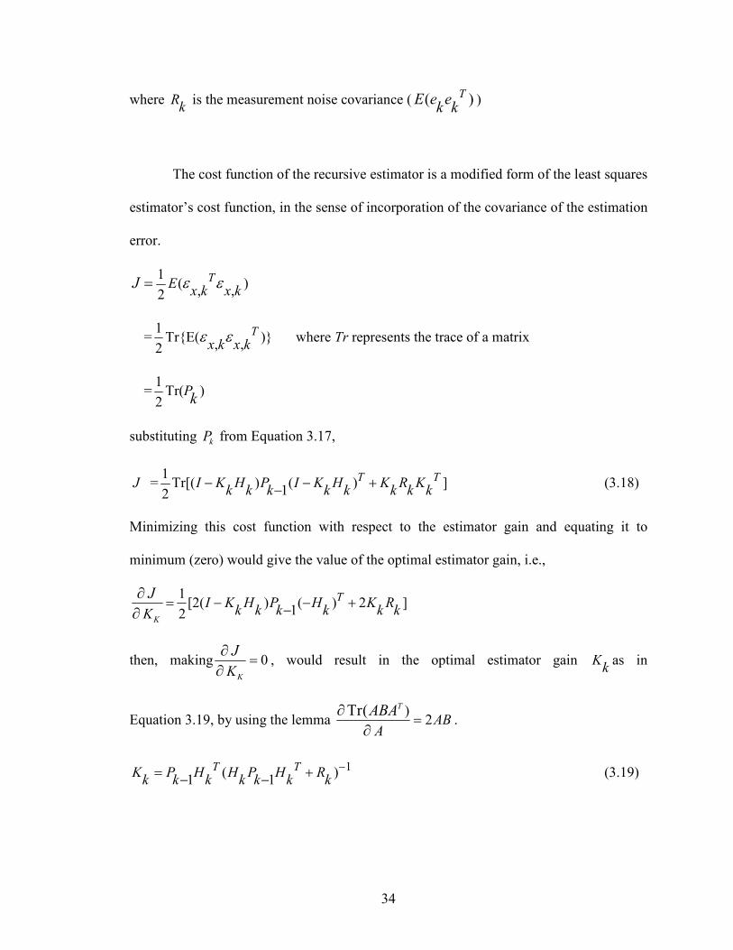
The cost function of the recursive estimator is a modified form of the least squares
estimator’s cost function, in the sense of incorporation of the covariance of the estimation
error.
1( )
, ,2
TEx k x k
J ε ε=
=1Tr{E( )}
, ,2
T
x k x kε ε where Tr represents the trace of a matrix
=1Tr( )
2Pk
substituting kP from Equation 3.17,
J =1Tr[( ) ( ) ]
12
T TI K H P I K H K R Kk k k k k k k k
− − +− (3.18)
Minimizing this cost function with respect to the estimator gain and equating it to
minimum (zero) would give the value of the optimal estimator gain, i.e.,
1[2( ) ( ) 2 ]
12K
TI K H P H K Rk k k k k kK
J= − − +−
∂∂
then, making 0KK
J=
∂∂
, would result in the optimal estimator gain Kkas in
Equation 3.19, by using the lemma )
2Tr( T
ABA
ABA=
∂∂
.
1( )1 1
T TK P H H P H Rk k k k k k k
−= +− − (3.19)
35
Though Equations 3.17 and 3.19 represent the estimator error covariance and
estimator gain, these are not the only derived equations that represent those values. There
may be other equations derived for these terms, but they can also be obtained by math
manipulations from the above equations.
3.2 State estimation in a linear system
Estimation of a constant vector was only discussed in the previous sections and
those estimation techniques can also be implemented for estimating the states of a
dynamic system. But since the estimated quantities may not be constant, the estimator
would tend to ignore information contained in the later measurements [16]. Hence, the
estimator should incorporate the additional information like the dynamic effects of the
system model and its inputs on the estimate ( ˆkx ) and its uncertainty, i.e., estimation error
covariance ( kP ). The inputs and initial conditions of a dynamic system are random, due
to which the state itself must be considered a random variable. This is where the
estimation is effected by the probabilistic functions of the variables. The propagation of
the state and its uncertainty through the time history, interpreted with the probabilistic
approach is explained for a discrete time linear time varying system in the following
example.
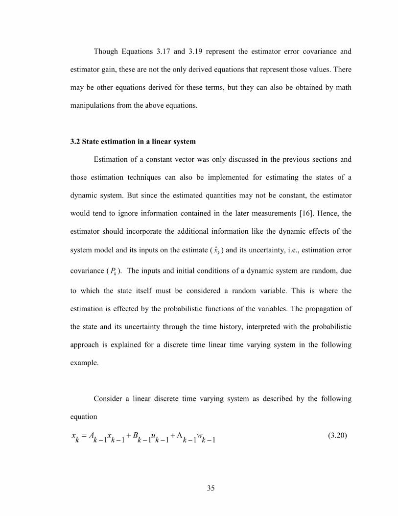
Consider a linear discrete time varying system as described by the following
equation
1 1 1 1 1 1k k k k k k kx A x B u w
− − − − − −= + +Λ (3.20)
36
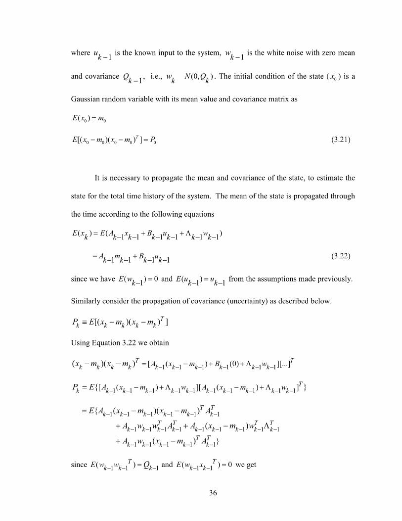
where 1k
u−
is the known input to the system, 1k
w−
is the white noise with zero mean
and covariance 1
Qk −
, i.e., (0, )N Qk kw � . The initial condition of the state ( 0x ) is a
Gaussian random variable with its mean value and covariance matrix as
0 0( )E x m=
0 0 0 0 0[( )( ) ]TE x m x m P− − = (3.21)
It is necessary to propagate the mean and covariance of the state, to estimate the
state for the total time history of the system. The mean of the state is propagated through
the time according to the following equations
( ) ( )1 1 1 1 1 1
E x E A x B u wk k k k k k k
= + +Λ− − − − − −
=1 1 1 1
A m B uk k k k
+− − − − (3.22)
since we have ( ) 01
E wk
=− and ( )1 1
E u uk k
=− − from the assumptions made previously.
Similarly consider the propagation of covariance (uncertainty) as described below.
[( )( ) ]Tk k k k kP E x m x m≡ − −
Using Equation 3.22 we obtain
1 1 1 1 1 1[ ( ) (0) ][...]( )( )T T
k k k k k k k k k kA x m B wx m x m − − − − − −= − + +Λ− −
1 1 1 1 1 1 1 1 1 1[ ( ) ][ ( ) ]{ }T
k k k k k k k k k k kA x m w A x m wP E − − − − − − − − − −− +Λ − +Λ=
1 1 1 1 1 1
1 1 1 1 1 1 1 1 1
1 1 1 1 1}
{ ( )( )
( )
( )
T Tk k k k k k
T T T Tk k k k k k k k k
T Tk k k k k
E A x m x m A
A w w A A x m w
A w x m A
− − − − − −
− − − − − − − − −
− − − − −
= − −
+ + − Λ
+ −
since 1 1 1
( )Tk k k
E w w Q− − −= and 1 1
( ) 0Tk k
E w x− − = we get
37
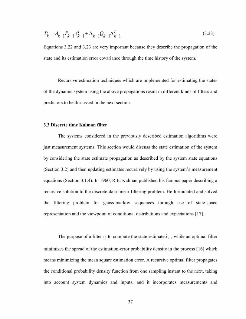
1 1 1 1 1 1T T
k k k k k k kP A P A Q− − − − − −= +Λ Λ (3.23)
Equations 3.22 and 3.23 are very important because they describe the propagation of the
state and its estimation error covariance through the time history of the system.
Recursive estimation techniques which are implemented for estimating the states
of the dynamic system using the above propagations result in different kinds of filters and
predictors to be discussed in the next section.
3.3 Discrete time Kalman filter
The systems considered in the previously described estimation algorithms were
just measurement systems. This section would discuss the state estimation of the system
by considering the state estimate propagation as described by the system state equations
(Section 3.2) and then updating estimates recursively by using the system’s measurement
equations (Section 3.1.4). In 1960, R.E. Kalman published his famous paper describing a
recursive solution to the discrete-data linear filtering problem. He formulated and solved
the filtering problem for gauss-markov sequences through use of state-space
representation and the viewpoint of conditional distributions and expectations [17].
The purpose of a filter is to compute the state estimate ˆkx , while an optimal filter
minimizes the spread of the estimation-error probability density in the process [16] which
means minimizing the mean square estimation error. A recursive optimal filter propagates
the conditional probability density function from one sampling instant to the next, taking
into account system dynamics and inputs, and it incorporates measurements and
38
measurement error statistics in the estimate [16]. As discussed in the previous section, the
state estimate ˆkx is specified by expected value (mean) of the true state’s ( kx ) conditional
probability density function and the spread of uncertainty in estimate is specified as the
covariance matrix. This recursive generation of the mean and covariance in finite time
can be explained in the following five steps:
1) State Estimate Extrapolation (Time Propagation)
2) Covariance Estimate Extrapolation (Time Propagation)
3) Filter Gain Computation
4) State Estimate Measurement Update
5) Covariance Estimate Measurement Update
The first two steps that describe the propagation of the estimate (mean) of the
state and its uncertainty (estimation error covariance) are already discussed in the
previous section of (Section 3.2). The last three steps can be performed by the recursive
(weighted) least squares estimation technique as discussed in that Section 3.1.4.
The mathematical form of the five steps performed in the Kalman filter can be
derived by considering a linear time varying discrete time stochastic system represented
by Equation 3.24a and 3.24b.
1 1 1 1 1 1k k k k k k kx A x B u w− − − − − −= + +Λ (3.24a)
k k k kz C x n= + (3.24b)
39
Equation 3.24a represents the state equation of the system with x as the state
vector, u as the control input to the system and w as the process noise in the system. This
process noise is considered to be a zero-mean white noise, Gaussian random variable
with Qkas its covariance.
( ) 0k
E w =
( )Tk k k
E w w Q= (3.25)
Equation 3.24b describes the measurement model of the system. z, the
measurement vector, is a combination of states x associated with some measurement
noise represented by n. Similar to the process noise, this noise n is also a zero-mean
white noise, Gaussian random variable with kR as its covariance.
( ) 0k
E n =
( )Tk k k
E n n R= (3.26)
The system matrices represented by A, B, C, and Λ are considered to be known.
The important assumption to be considered is that the process noise and measurement
noise are independent, i.e., there is no correlation existing between them.
0( ) ( )T Tw nk k k k
E n E w= = (3.27)
It is also assumed that values of the initial state estimate 0x̂ and initial estimation
error covariance 0P are known beforehand as discussed in Section 3.2.
40
0 0ˆ ( )x E x= and
0 0 0 0 0ˆ ˆ[( )( ) ]TP E x x x x= − −
There are two main transitions to be considered for the propagation of any
variable of the system through the time instants. They are state update and measurement
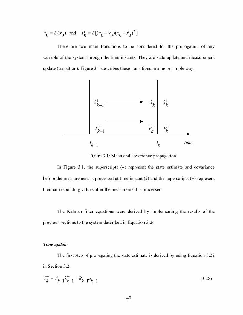
update (transition). Figure 3.1 describes these transitions in a more simple way.
ˆ1
xk+− x̂
k− x̂
k+
1k
P+− kP−
kP+
1k
t − kt time
Figure 3.1: Mean and covariance propagation
In Figure 3.1, the superscripts (−) represent the state estimate and covariance
before the measurement is processed at time instant (k) and the superscripts (+) represent
their corresponding values after the measurement is processed.
The Kalman filter equations were derived by implementing the results of the
previous sections to the system described in Equation 3.24.
Time update
The first step of propagating the state estimate is derived by using Equation 3.22
in Section 3.2.
1 1 1 1ˆ ˆk k k k kx A x B u− +
− − − −= + (3.28)
41
Similar to the above step, estimation error covariance is propagated with time
according to the Equation 3.23 in Section 3.2.
1 1 1 1 1 1T T
k k k k k k kP A P A Q− +
− − − − − −= +Λ Λ (3.29)
Measurement update
Now that ˆkx− is calculated, ˆ
kx+ (which is the state estimate obtained after the
measurement update) is calculated using the RLS estimation technique as discussed in
Section 3.1.4.
We calculate the Kalman gain from Equation 3.19, but in this case 1k
P − is
replaced by kP− which represents the estimation error covariance before the
measurements are obtained.
1[ ]T Tk k k k k k k
K P C C P C R −− −= + (3.30)
Using the above Kalman gain, the state estimate and estimate error covariance are
updated after processing the measurements as discussed in Section 3.1.4. But in this case
1ˆkx − is replaced by ˆ
kx− ,
1kP − is replaced by
kP− , ˆ
kx is replaced by ˆ
kx+ and
kP is
replaced by kP+ in the Equations 3.15 and 3.17.
ˆ ˆ ˆ( )k k k k k kx x K z C x+ − −= + − (3.31)
( ) ( )T Tk k k k k k k k kP I K C P I K C K R K+ −= − − + (3.32)
42
The last five equations represent the fundamental Kalman filter equations;
however there are different forms for these KF equations which are obtained by
manipulating the above equations with some linear algebra. The important property of the
Kalman filter is that it’s a linear filter and it can estimate the states of a linear system
only. However, it can be extended to a nonlinear system by linearizing the system which
will be discussed in Chapter IV. The Kalman filter is considered to be the best linear
filter in estimating the states of a system with both process and measurement noise, i.e., w
and n, are uncorrelated and white. The quantity ˆ( )k k kz C x−− used to update the state
estimate in Equation 3.31 is called the innovations. The same concept can be extended to
continuous time systems too. Many other filters are designed based on these basic
Kalman filter equations, like
1) Steady state KF
2) Constrained KF
3) Robust KF
4) Square root KF
5) Sequential KF
These filters work similar to the fundamental Kalman filter. In the steady state KF
a steady state gain is used for propagating the estimate and its error covariance through
time. A Kalman filter designed with certain constraints on the estimates is called the
constrained KF [10]. The robust KF addresses uncertainties in the process and
measurement noise covariances and gives better results than the standard Kalman
filter [19]. Similarly, the other Kalman filters incorporate certain other factors in
estimating the states.
43
CHAPTER IV
LINEARIZED KALMAN FILTER
The estimation techniques discussed in the previous chapter can only be applied to linear
systems. However, most physical systems encountered in nature are nonlinear systems.
For several reasons, the problem of filtering and smoothing for nonlinear systems is
considerably more difficult and admits a wider variety of solutions than does the linear
estimation problem [15]. This difficulty arises because of the nonlinear elements in the
systems which alter the probability density function of signals and noise as they are
transmitted through the time, i.e., Gaussian inputs cause non-Gaussian response. The
shapes of the distributions change when probability density functions are transmitted
through nonlinear elements. Fortunately, estimators for many nonlinear systems can be
derived based on basic Kalman filter as stated in the previous chapter; though not
precisely “optimum”, they are “optimal” in the sense that they tend to the optimum.
Section 4.1 discusses nonlinear estimation along with different nonlinear estimation
techniques. Linearization process and different linearization techniques are explained in
Section 4.2. Sections 4.3 and 4.4 discuss linearization and discretization of the turbofan
44
engine model (MAPSS) used in this research. An alternate equivalent Kalman filter (a
priori) equations are derived in Section 4.5. Finally, Section 4.6 discusses the graphical
user interface developed for the turbofan health parameter estimation.
4.1 Nonlinear estimation
The basic design of any (recursive) filter is based on the propagation of the state
estimate and its error covariance through the system. In linear systems, the state estimate
which is a GRV (Gaussian random variable) is transmitted linearly but transmitting the
Gaussian through nonlinear elements doesn’t give the same shape of the distribution.
There are basically two types of propagations of mean and variance through nonlinear
systems. The first type involves propagating the state estimate analytically through the
first order linearization of the nonlinear system. Linearized Kalman filter, extended
Kalman filter and hybrid extended Kalman filter use this type of propagation. The second
type involves approximating the state distribution by a small set of carefully chosen
sample points and then propagating these sample points through the true nonlinear
system. Unscented Kalman filter, a new nonlinear estimation algorithm, is the result of
the second type of propagation. UKF is discussed in detail in the Chapter VI.
4.1.1 Linearized Kalman filter
Linearized Kalman filter and extended Kalman filter are mainly based on the
linearization of the systems which will be discussed in the Section 4.2. Consider a
nonlinear system described by the following equations.
45
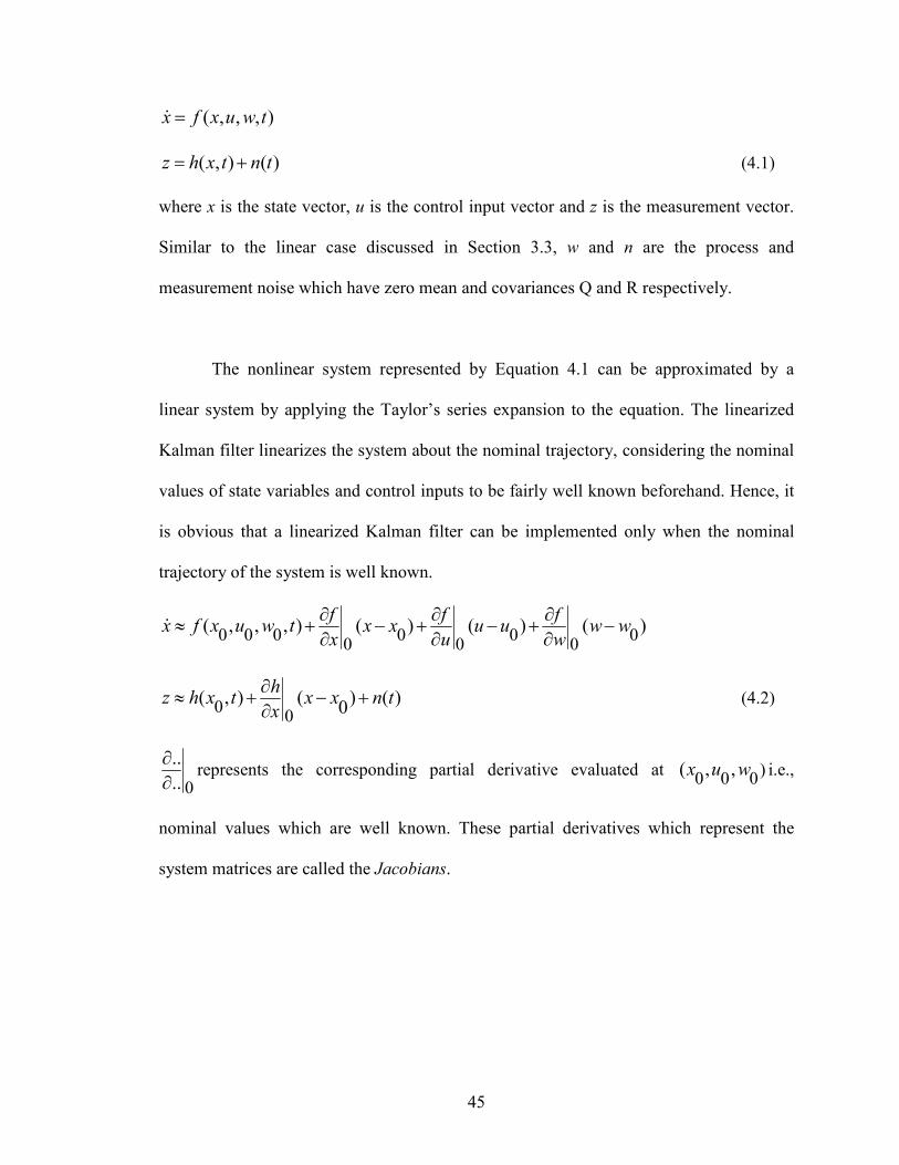
( , , , )x f x u w t=&
( , ) ( )z h x t n t= + (4.1)
where x is the state vector, u is the control input vector and z is the measurement vector.
Similar to the linear case discussed in Section 3.3, w and n are the process and
measurement noise which have zero mean and covariances Q and R respectively.
The nonlinear system represented by Equation 4.1 can be approximated by a
linear system by applying the Taylor’s series expansion to the equation. The linearized
Kalman filter linearizes the system about the nominal trajectory, considering the nominal
values of state variables and control inputs to be fairly well known beforehand. Hence, it
is obvious that a linearized Kalman filter can be implemented only when the nominal
trajectory of the system is well known.
0 0 0 0 0 00 0 0
( , , , ) ( ) ( ) ( )f f f
x f x u w t x x u u w wx u w
∂ ∂ ∂≈ + − + − + −
∂ ∂ ∂&
00
( , ) ( ) ( )0
hz h x t x x n t
x
∂≈ + − +
∂ (4.2)
0
..
..
∂∂
represents the corresponding partial derivative evaluated at )0 0 0
( , ,x u w i.e.,
nominal values which are well known. These partial derivatives which represent the
system matrices are called the Jacobians.
46
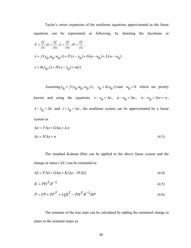
Taylor’s series expansion of the nonlinear equations approximated as the linear
equations can be represented as following, by denoting the Jacobians as
, , ,f f f f
F G L Hx u w x
∂ ∂ ∂ ∂= = = =∂ ∂ ∂ ∂
.
0 0 0 0 0 0( , , , ) ( ) ( ) ( )x f x u w t F x x G u u L w w= + − + − + −&
0 0( , ) ( ) ( )z h x t H x x n t= + − +
Assuming0 0 0 0
( , , , )x f x u w t=& , ( ,0 0
)hz x t= and 00w = which are priorly
known and using the equations 0
x x x− = ∆ , 0
u u u− = ∆ , 0
w w w w− = ∆ = ,
0x x x− = ∆& & & and
0z z z− = ∆ , the nonlinear system can be approximated by a linear
system as
x F x G u Lw∆ = ∆ + ∆ +&
z H x n∆ = ∆ + (4.3)
The standard Kalman filter can be applied to the above linear system and the
change in states ( x̂∆ ) can be estimated as
ˆ ˆ ˆ( )x F x G u K z H x∆ = ∆ + ∆ + ∆ − ∆& (4.4)
1TK PH R−= (4.5)
1T T TP FP PF LQL PH R HP−= + + −& (4.6)
The estimate of the true state can be calculated by adding the estimated change in
states to the nominal states as
47
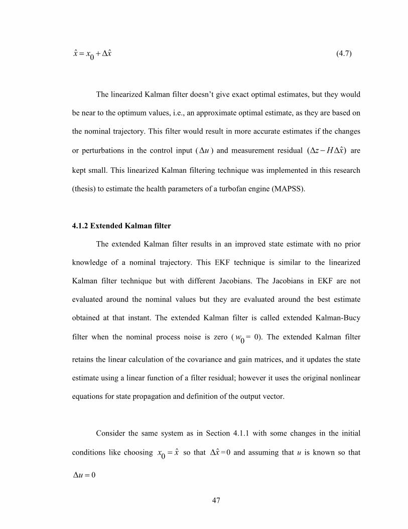
0ˆ ˆx x x= +∆ (4.7)
The linearized Kalman filter doesn’t give exact optimal estimates, but they would
be near to the optimum values, i.e., an approximate optimal estimate, as they are based on
the nominal trajectory. This filter would result in more accurate estimates if the changes
or perturbations in the control input ( u∆ ) and measurement residual ˆ( )z H x∆ − ∆ are
kept small. This linearized Kalman filtering technique was implemented in this research
(thesis) to estimate the health parameters of a turbofan engine (MAPSS).
4.1.2 Extended Kalman filter
The extended Kalman filter results in an improved state estimate with no prior
knowledge of a nominal trajectory. This EKF technique is similar to the linearized
Kalman filter technique but with different Jacobians. The Jacobians in EKF are not
evaluated around the nominal values but they are evaluated around the best estimate
obtained at that instant. The extended Kalman filter is called extended Kalman-Bucy
filter when the nominal process noise is zero (0w = 0). The extended Kalman filter
retains the linear calculation of the covariance and gain matrices, and it updates the state
estimate using a linear function of a filter residual; however it uses the original nonlinear
equations for state propagation and definition of the output vector.
Consider the same system as in Section 4.1.1 with some changes in the initial
conditions like choosing 0
ˆx x= so that x̂∆ =0 and assuming that u is known so that
0u∆ =
48
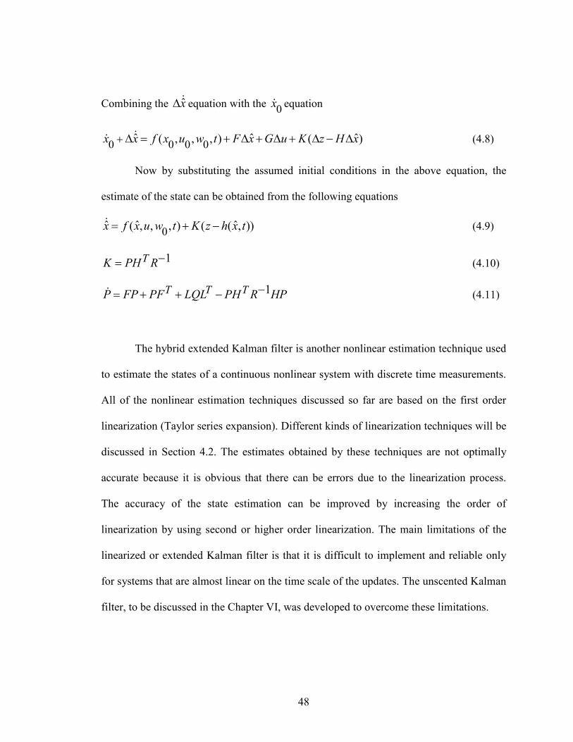
Combining the x̂∆& equation with the 0x& equation
0 0 0 0ˆ ˆ ˆ( , , , ) ( )x x f x u w t F x G u K z H x+∆ = + ∆ + ∆ + ∆ − ∆&& (4.8)
Now by substituting the assumed initial conditions in the above equation, the
estimate of the state can be obtained from the following equations
0ˆ ˆ ˆ( , , , ) ( ( , ))x f x u w t K z h x t= + −& (4.9)
1TK PH R−= (4.10)
1T T TP FP PF LQL PH R HP−= + + −& (4.11)
The hybrid extended Kalman filter is another nonlinear estimation technique used
to estimate the states of a continuous nonlinear system with discrete time measurements.
All of the nonlinear estimation techniques discussed so far are based on the first order
linearization (Taylor series expansion). Different kinds of linearization techniques will be
discussed in Section 4.2. The estimates obtained by these techniques are not optimally
accurate because it is obvious that there can be errors due to the linearization process.
The accuracy of the state estimation can be improved by increasing the order of
linearization by using second or higher order linearization. The main limitations of the
linearized or extended Kalman filter is that it is difficult to implement and reliable only
for systems that are almost linear on the time scale of the updates. The unscented Kalman
filter, to be discussed in the Chapter VI, was developed to overcome these limitations.
49
4.2 Linearization
Linearization is the process of modeling a nonlinear system as a linear system.
The linear model is an idealized or simplified version of the more accurate (but more
complicated) nonlinear model. The linear mathematical model can then be used in the
many analysis and design tools that require a linear model. The linear model accurately
represents the dynamics of the nonlinear system at certain operating conditions, but may
not be accurate at other operating conditions.
In control engineering, the normal operation of the system may be around an
equilibrium point, and the system signals can be considered small deviations around the
equilibrium. In this case, it can be useful to approximate the nonlinear system with a
linear system. The linear model is approximately equivalent to the nonlinear system if the
operating range remains near the linearization point. Linearized models are very
important in control engineering. In general, there are many more tools for applying
control and estimation techniques to linear systems than there are for nonlinear systems.
There are different linearization techniques that can be performed on nonlinear systems.
Almost all the linearization techniques are based on Taylor series expansions. The
linearization methods that are explored in this chapter (section) are listed below
1) Matlab Linearization
2) Perturbation Linearization
3) Steady State Error Reduction
The accuracy of these linearization methods relative to MAPSS model fidelity
and turbofan engine health parameter estimation is investigated.
50
4.2.1 Matlab Linearization
A nonlinear model can be linearized directly using MATLAB [12] functions such
as linmod, dlinmod and linmod2. The equilibrium or operating point is calculated by
using MATLAB’s trim function. The trim function finds out the equilibrium point at
which the system is at steady state; i.e., the state derivatives are zero. If there is no point
at which the system is at steady state, then the trim function will give the point at which
the state derivative is nearest to 0. MATLAB’s trim function is invoked as follows.
[x, u, y] = trim (‘sys’, 0x , 0u , 0y ) (4.12)
where x, u, and y are the output equilibrium points for the system described by ‘sys,’ and
0x , 0u , and 0y are the user’s initial guess for the equilibrium points.
The linmod function obtains a linear model from a system of ordinary differential
equations that are implemented as a Simulink [13] model. The dlinmod function can
linearize discrete, multirate, and hybrid continuous-time and discrete-time systems at any
given sampling time. This is usually used for linearizing discrete-time systems. The
linmod function is invoked as follows.
[A, B, C, D] = linmod (‘sys’, x, u) (4.13)
where x and u are the outputs of the trim function. This gives the linearized model of
system ‘sys’ (in A, B, C, and D matrices) around the specified operating point.
51
4.2.2 Perturbation Linearization
A nonlinear system can be represented by the following state space equations.
( , , )x f x u t=&
( , , )y h x u t= (4.14)
where f and h are nonlinear functions, x is the state vector, u is the control vector, and y is
the output vector. The nonlinear system is run in closed loop until it reaches steady state
(i.e., x& =0). Once the system reaches steady state, the resulting state vector 0x , input
vector 0u , and output vector 0y are saved as the nominal values.
4.2.2a Linearization with respect to states
Each state is perturbed individually, and the corresponding changes in the state
derivatives and output vectors are calculated. The nonlinear system represented by
Equation 4.14 can be linearized to the system described by following equations.
x A x B u
y C x D u
∆ = ∆ + ∆∆ = ∆ + ∆
& (4.15)
where columns of the A and C matrices are calculated by using the following equations.
change in element of vectorthix i x∆ =
change in vector due to changein (at the initial time)1 1
(at the initial time)change in vector due tochangeinn n
x x x
x x x
=
=
∆
∆M M
& &
& &
21
0 0 01
0[ ]
0 n
x
xx x An
x
∆
∆∆ ∆ =
∆
LL
M& &L
M O M
LLLLL
52
111 1
2
1
0 0 0
0
0
n
nnn n
xA A
x
A A x
=
∆
∆
∆
L LLLL
MM M
M M M O M
LLL LLLLL
11 1 1
1 1
nn
nn nn
A x A x
A x A x
∆ ∆
=
∆ ∆
LL
M M
M M
LL
(1 column of )1 1
( columnof )
st
th
A
n An n
x x
x x
= ×
= ×
∆ ∆
∆ ∆
M M
&
&
column of /th A i ii x x=∆ ∆&
The ith columns of the A and C matrices are computed as follows.
(:, ) ( 0) /( ( ) 0( ))
(:, ) ( 0) /( ( ) 0( ))
A i x x x i x i
C i y y x i x i
= − −
= − −
& & (4.16)
this is performed for i = 1, …, n where n is the number of states of the system.
4.2.2b Linearization with respect to control inputs
Similar to linearization with respect to states in Section 4.2.2a, the control inputs
are perturbed individually and the corresponding changes in the state derivatives and
output vectors are calculated. Then the ith column of the B and D matrices are calculated
as follows.
(:, ) ( 0) /( ( ) 0( ))
(:, ) ( 0) /( ( ) 0( ))
B i x x u i u i
D i y y u i u i
= − −= − −
& & (4.17)
This is done for i = 1, …, p where p is the number of controls of the system.
53
4.2.3 Steady state error reduction method
The steady state error reduction method results a steady state error of zero
between the linear and nonlinear models (under certain conditions). This method is often
better than the Matlab or perturbation methods.
4.2.3a Linearization with respect to states
The nonlinear system represented by Equation 4.14 is run in closed loop until it
reaches steady state. Then the steady state control inputs, states, and outputs are saved for
later calculations (these are referred to as the nominal inputs, states, and outputs). Each
state element is perturbed individually from their nominal values by some small
percentage and then corresponding changes in the states, state derivatives, and outputs are
observed at some small time greater than zero. The state, state derivative and output
changes are saved as column vectors. After this procedure is repeated for each state
element, the column vectors are augmented to form matrices. Then using the following
equations, A and C matrices are computed.
0u∆ = ; i.e., control inputs are not changed
change in vector due tochange ini ix x x=∆
change in vector (at somesmallnonzero time)due tochangeini ix x x=∆& &
1[ ]nx x x∆ = ∆ ∆L
1[ ]nx x x∆ = ∆ ∆& & &L
1 1
n n
x A x
x A x
∆ = ∆
∆ = ∆
&
M
&
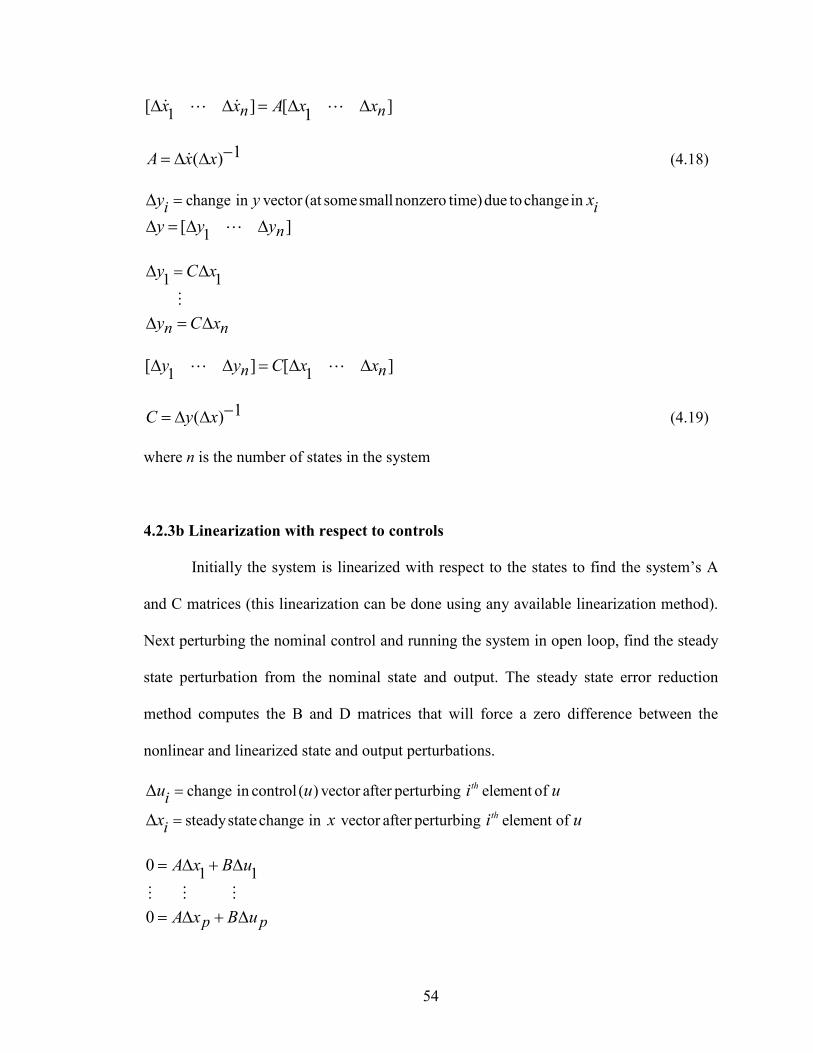
54
1[ ] [ ]
1n nx x A x x∆ ∆ = ∆ ∆& &L L
1( )A x x −= ∆ ∆& (4.18)
change in vector (at somesmallnonzero time)due tochangeini iy y x=∆
1[ ]ny y y∆ = ∆ ∆L
1 1
n n
y C x
y C x
=∆ ∆
∆ = ∆M
1 1[ ] [ ]n ny y C x x∆ ∆ = ∆ ∆L L
1( )C y x −= ∆ ∆ (4.19)
where n is the number of states in the system
4.2.3b Linearization with respect to controls
Initially the system is linearized with respect to the states to find the system’s A
and C matrices (this linearization can be done using any available linearization method).
Next perturbing the nominal control and running the system in open loop, find the steady
state perturbation from the nominal state and output. The steady state error reduction
method computes the B and D matrices that will force a zero difference between the
nonlinear and linearized state and output perturbations.
change in control ( ) vector after perturbing element of
steadystatechange in vector after perturbing element of
th
th
i
i
u u i u
x x i u
=
=
∆
∆
1 10
0 p p
A x B u
A x B u
= ∆ + ∆
= ∆ + ∆M M M
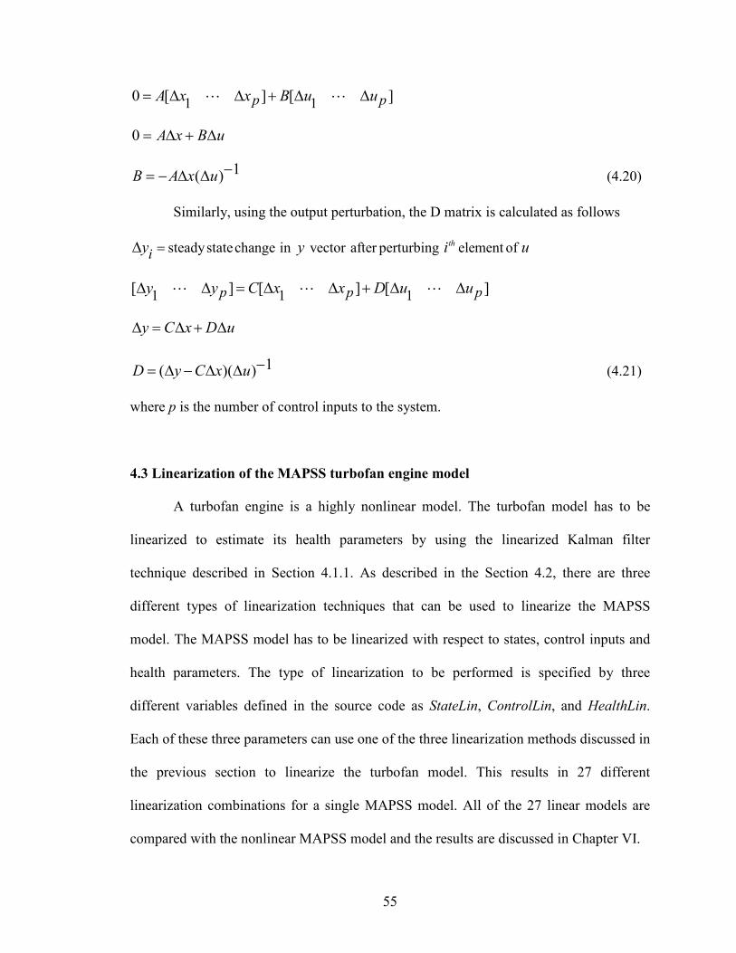
55
1 10 [ ] [ ]p pA x x B u u= ∆ ∆ + ∆ ∆L L
0 A x B u= ∆ + ∆
1( )B A x u −= − ∆ ∆ (4.20)
Similarly, using the output perturbation, the D matrix is calculated as follows
steadystatechange in vector after perturbing element ofth
iy y i u=∆
1 1 1[ ] [ ] [ ]p p py y C x x D u u∆ ∆ = ∆ ∆ + ∆ ∆L L L
y C x D u∆ = ∆ + ∆
1( )( )D y C x u −= ∆ − ∆ ∆ (4.21)
where p is the number of control inputs to the system.
4.3 Linearization of the MAPSS turbofan engine model
A turbofan engine is a highly nonlinear model. The turbofan model has to be
linearized to estimate its health parameters by using the linearized Kalman filter
technique described in Section 4.1.1. As described in the Section 4.2, there are three
different types of linearization techniques that can be used to linearize the MAPSS
model. The MAPSS model has to be linearized with respect to states, control inputs and
health parameters. The type of linearization to be performed is specified by three
different variables defined in the source code as StateLin, ControlLin, and HealthLin.
Each of these three parameters can use one of the three linearization methods discussed in
the previous section to linearize the turbofan model. This results in 27 different
linearization combinations for a single MAPSS model. All of the 27 linear models are
compared with the nonlinear MAPSS model and the results are discussed in Chapter VI.
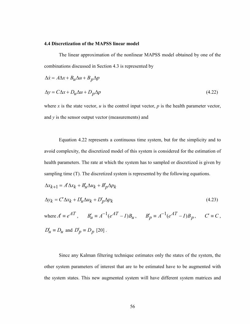
56
4.4 Discretization of the MAPSS linear model
The linear approximation of the nonlinear MAPSS model obtained by one of the
combinations discussed in Section 4.3 is represented by
u px A x B u B p∆ = ∆ + ∆ + ∆&
u py C x D u D p∆ = ∆ + ∆ + ∆ (4.22)
where x is the state vector, u is the control input vector, p is the health parameter vector,
and y is the sensor output vector (measurements) and
Equation 4.22 represents a continuous time system, but for the simplicity and to
avoid complexity, the discretized model of this system is considered for the estimation of
health parameters. The rate at which the system has to sampled or discretized is given by
sampling time (T). The discretized system is represented by the following equations.
1k k u k p kx A x B u B p+ ′ ′ ′∆ = ∆ + ∆ + ∆
k k u k p ky C x D u D p′ ′ ′∆ = ∆ + ∆ + ∆ (4.23)
whereATA e′ ≡ ,
1( )ATu uB A e I B−′ ≡ − ,
1( )ATp pB A e I B−′ ≡ − , C C′ ≡ ,
u uD D′ ≡ and p pD D′ ≡ [20] .
Since any Kalman filtering technique estimates only the states of the system, the
other system parameters of interest that are to be estimated have to be augmented with
the system states. This new augmented system will have different system matrices and
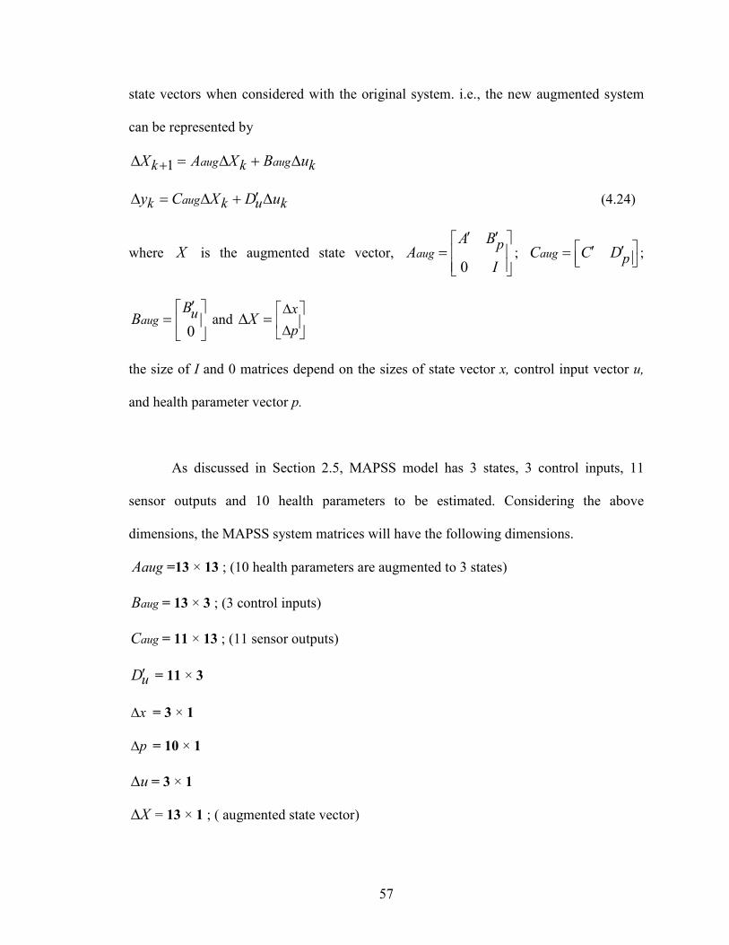
57
state vectors when considered with the original system. i.e., the new augmented system
can be represented by
1 aug augk k kX A X B u+∆ = ∆ + ∆
augk k u ky C X D u′∆ = ∆ + ∆ (4.24)
where X is the augmented state vector, 0
augpA B
AI
′ ′= ; aug pC C D
′ ′= ;
0aug
uBB
′= and
x
pX
∆ ∆
∆ =
the size of I and 0 matrices depend on the sizes of state vector x, control input vector u,
and health parameter vector p.
As discussed in Section 2.5, MAPSS model has 3 states, 3 control inputs, 11
sensor outputs and 10 health parameters to be estimated. Considering the above
dimensions, the MAPSS system matrices will have the following dimensions.
augA =13 × 13 ; (10 health parameters are augmented to 3 states)
augB = 13 × 3 ; (3 control inputs)
augC = 11 × 13 ; (11 sensor outputs)
uD′ = 11 × 3
x∆ = 3 × 1
p∆ = 10 × 1
u∆ = 3 × 1
X∆ = 13 × 1 ; ( augmented state vector)
58
The linearized Kalman filter technique is implemented on this augmented system
to estimate the augmented state vector X∆ .
4.5 Discrete Linearized Kalman filter
The linearized Kalman filter discussed in Section 4.1.1 was for continuous time
systems. However, for simplicity and reducing the complexity, the discrete model of the
turbofan model is used in this research. The discretized form of the linearized Kalman
filter uses the same five equations as discussed in Section 3.3 in the previous chapter
except for the system matrices (A, B, C and D) are obtained by linearizing the nonlinear
turbofan model at the nominal values. There are different equivalent Kalman filter
equations that can be implemented in a more simple way compared to the conventional
Kalman filter.
The type of linearized Kalman filter implemented in this research is the a priori
Kalman filter. The typical five equations are reduced to three equations in this a priori
filter. An a priori filter is one in which states and estimation error covariances are
updated using their a priori values i.e., ˆkx− and
kP− .
Considering Equation 4.26 in Section 3.3 for a priori estimation error covariance we see
that
1 1 1 1T
k k k k kP A P A Q− +
− − − −′= + where
1 1 1 1T
k k k kQ Q≡− − − −′ Λ Λ
The Kalman gain from Section 3.3 (Equation 4.27) is
59
1[ ]T Tk k k k k k k
K P C C P C R −− −= +
then by substituting the value of a posteriori value for estimation error covariance 1k
P+−
from Section 3.3 (Equation 4.29), the following equation is obtained.
1 1 1 1 1 1 1 1 1T TC
k k k k k k k k k kP A P A A K P A Q− − −− +− − − − − − − − −
′=
From 1 1 1k k k
K A K≡− − −′ we obtain
11 1 1 1 1 1 1 1
[ ]T Tk k k k k k k k
K A P C C P C R −− − − − − − − −
− −′ = + (4.25)
The a priori value of estimation error covariance is
1 1 1 1 1 1 1 1T TC
k k k k k k k k kP A P A K P A Q− − −− +− − − − − − − −
′ ′= (4.26)
Now considering the state estimate update equations from Section 3.3, i.e.,
(Equation 4.25) we obtain
1 1 1 1ˆ ˆk k k k kx A x B u− +
− − − −= +
Substituting the a posteriori estimate 1
ˆkx+− from Equation 4.28 gives
( )1 1 1 1 1 1 1 1
ˆ ˆ ˆk k k k k k k k kx A x B u K z C x− − −+− − − − − − − −
′= + − (4.27)
Equations 4.25, 4.26 and 4.27 represent the a priori Kalman filter which are
implemented in this research. The state estimate and estimation error covariance are
updated using these three equations. The above derivations are discussed in more detail
in [21].

60
4.6 Health estimation GUI
A graphical user interface is developed for the health estimation of a turbofan
engine. This GUI is developed using Matlab’s GUIDE software. Like any other GUI, the
main aim of this health estimation GUI is to make the estimation process more user
friendly. Figure 4.1 displays the health estimation GUI of a turbofan engine. The user can
specify the estimation specifications like the type of estimation technique to be used, the
type of constraint to be implemented and also the type of filter, like steady state or time
varying. The linearization technique to be implemented can be specified using the linear
model push button. Initial conditions like initial estimation error covariance and process
noise covariance can also be specified.
The measurements that are to be used to estimate the health parameters can be
selected from the sensor outputs. The user can select sensor outputs of interest or the
default sensor set that is used in this research. Once the estimation is done, the estimation
errors are displayed in the text box at the bottom along with the estimation technique.
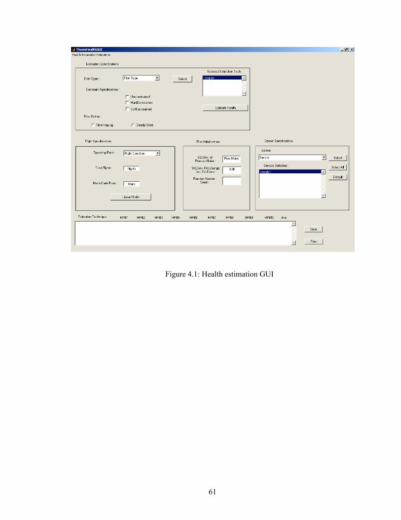
61
Figure 4.1: Health estimation GUI
62
CHAPTER V
SIMULATION RESULTS
The turbofan engine model is a highly nonlinear model. The model can be linearized so
that the nonlinear estimation techniques can be implemented to estimate the model’s
health parameters. As discussed in Chapter IV, there are three different types of
linearization techniques that can be used to linearize the MAPSS model. The type of
linearization to be performed is specified by three different variables defined in the code
as StateLin, ControlLin, and HealthLin. The linear models obtained are validated by
comparing the trend of certain variables in the linear models with those in the nonlinear
models over a period of time. Section 5.1 discusses the filtering results obtained from
different linear models and their validation. The linearized Kalman filter was
implemented on the MAPSS model to estimate the health parameters using all of the
possible linear models. Both the unconstrained and constrained forms of the linearized
Kalman filter estimates of the health parameters are shown in Section 5.2.
63
5. 1 Linearization of the MAPSS turbofan engine model
The MAPSS model was linearized with respect to states, control inputs and health
parameters and each of these variables could be linearized in one of the three
linearization techniques as discussed. This resulted in 27 different combinations of
linearization techniques that can be applied to a single nonlinear MAPSS model.
The linearization method that is used is specified by the parameters StateLin,
ControlLin, and HealthLin in the mapss_gui.m file. Each of these three parameters can be
linearized in one of the three ways that we discussed previously.
States 0. Perturbation method
1. Matlab method
2. Steady state error reduction method
Controls 0. Perturbation method
1. Matlab method
2. Steady state error reduction method
Health Parameters 0. Perturbation method
1. Matlab method
2. Steady state error reduction method
Three values have been assigned to each of these parameters (StateLin, ControlLin, and
HealthLin) to describe how they would be linearized. For instance, the Perturbation
Method is specified with a parameter value of 0, the Matlab method is specified with a
parameter value of 1, and the Steady state error reduction method is specified with a
parameter value of 2.
64
Validation
All 27 models were compared with the nonlinear model. The linear model that
resulted in minimum errors or deviations of the 22 sensor outputs from the nonlinear
model is the best linearized model of all the 27 combinations. This linearization test is
performed by perturbing the health parameters and initial states by some percentage of
their initial values. If there was no perturbation then both the linear and nonlinear model
would behave identically.
Each linearization technique can be used with a different perturbation value. We
used three different linearization perturbation values (0.01%, 0.1% and 0.5% of the
steady state value). We then tested the linear models that resulted with three different test
perturbation values (0.01%, 0.1% and 0.5%). There are two types of errors that we
considered for the validation of the linearization.
a) RMS Average Error
b) RMS Final Error
RMS average error is the average of the error over the whole time of the simulation (six
seconds), and the RMS Final error is the error at the final time of simulation (i.e., at time
= six seconds). The following tables show the best linearization method for each
combination of linearization perturbation and test perturbation.
In Tables I and II, LINxyz represents one of 27 linearization combinations.
x = StateLin (0, 1, or 2)
y = ControlLin (0, 1, or 2)
z = HealthLin (0, 1, or 2)
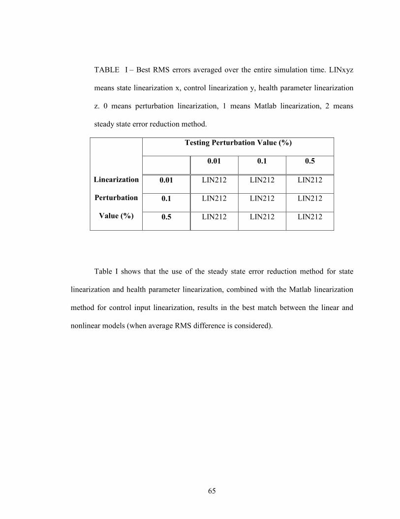
65
TABLE I – Best RMS errors averaged over the entire simulation time. LINxyz
means state linearization x, control linearization y, health parameter linearization
z. 0 means perturbation linearization, 1 means Matlab linearization, 2 means
steady state error reduction method.
Testing Perturbation Value (%)
0.01 0.1 0.5
0.01 LIN212 LIN212 LIN212
0.1 LIN212 LIN212 LIN212
Linearization
Perturbation
Value (%) 0.5 LIN212 LIN212 LIN212
Table I shows that the use of the steady state error reduction method for state
linearization and health parameter linearization, combined with the Matlab linearization
method for control input linearization, results in the best match between the linear and
nonlinear models (when average RMS difference is considered).
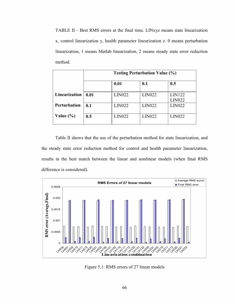
66
TABLE II – Best RMS errors at the final time. LINxyz means state linearization
x, control linearization y, health parameter linearization z. 0 means perturbation
linearization, 1 means Matlab linearization, 2 means steady state error reduction
method.
Testing Perturbation Value (%)
0.01 0.1 0.5
0.01 LIN022 LIN022 LIN122
LIN022
0.1 LIN022 LIN022 LIN022
Linearization
Perturbation
Value (%) 0.5 LIN022 LIN022 LIN022
Table II shows that the use of the perturbation method for state linearization, and
the steady state error reduction method for control and health parameter linearization,
results in the best match between the linear and nonlinear models (when final RMS
difference is considered).
RMS Errors of 27 linear models
0
0.0005
0.001
0.0015
0.002
0.0025
Lin000
Lin001
Lin002
Lin010
Lin011
Lin012
Lin020
Lin021
Lin022
Lin100
Lin101
Lin102
Lin110
Lin111
Lin112
Lin120
Lin121
Lin122
Lin200
Lin201
Lin202
Lin210
Lin211
Lin212
Lin220
Lin221
Lin222
Linearization combination
RMS error (A
verage,Final)
Average RMS ecrror
Final RMS error
Figure 5.1: RMS errors of 27 linear models
67
The linearization techniques can be grouped into two categories based on the
value of RMS errors as shown in Figure 5.1. All the linearization techniques in which the
model is linearized with respect to health parameters in the Matlab method resulted in the
worst RMS errors (LINxy1). All the other linearization techniques except the above case
give similar results. It can also be observed that error bars exhibit a sequential pattern for
all linearization techniques with a range of medium, high and low errors consecutively
for sequential three linear combinations (bars in Figure 5.1).
Figure 5.2 shows the behavior of four different parameters of the linearized model
(LIN002) with their corresponding nonlinear behavior. The solid lines represent the
nonlinear behavior and dashed lines represent the linear behavior of the same parameter.
Ground term in the label means that the engine is operated at the 1st operating point (PLA
= 21, mach number = 0, altitude = 0) and dpPct specifies the percentage of perturbation
in the health parameters by which the model is linearized. As seen there is not much
variation in the trend of the parameters in the linear and nonlinear case.
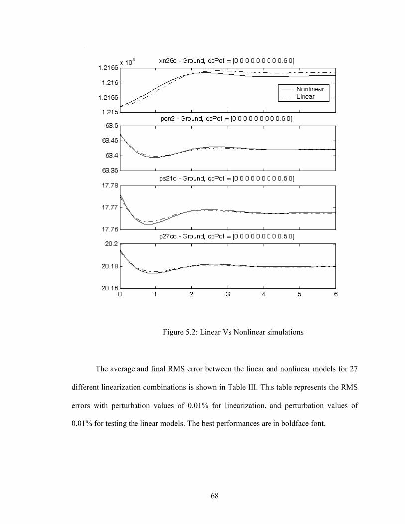
68
Figure 5.2: Linear Vs Nonlinear simulations
The average and final RMS error between the linear and nonlinear models for 27
different linearization combinations is shown in Table III. This table represents the RMS
errors with perturbation values of 0.01% for linearization, and perturbation values of
0.01% for testing the linear models. The best performances are in boldface font.
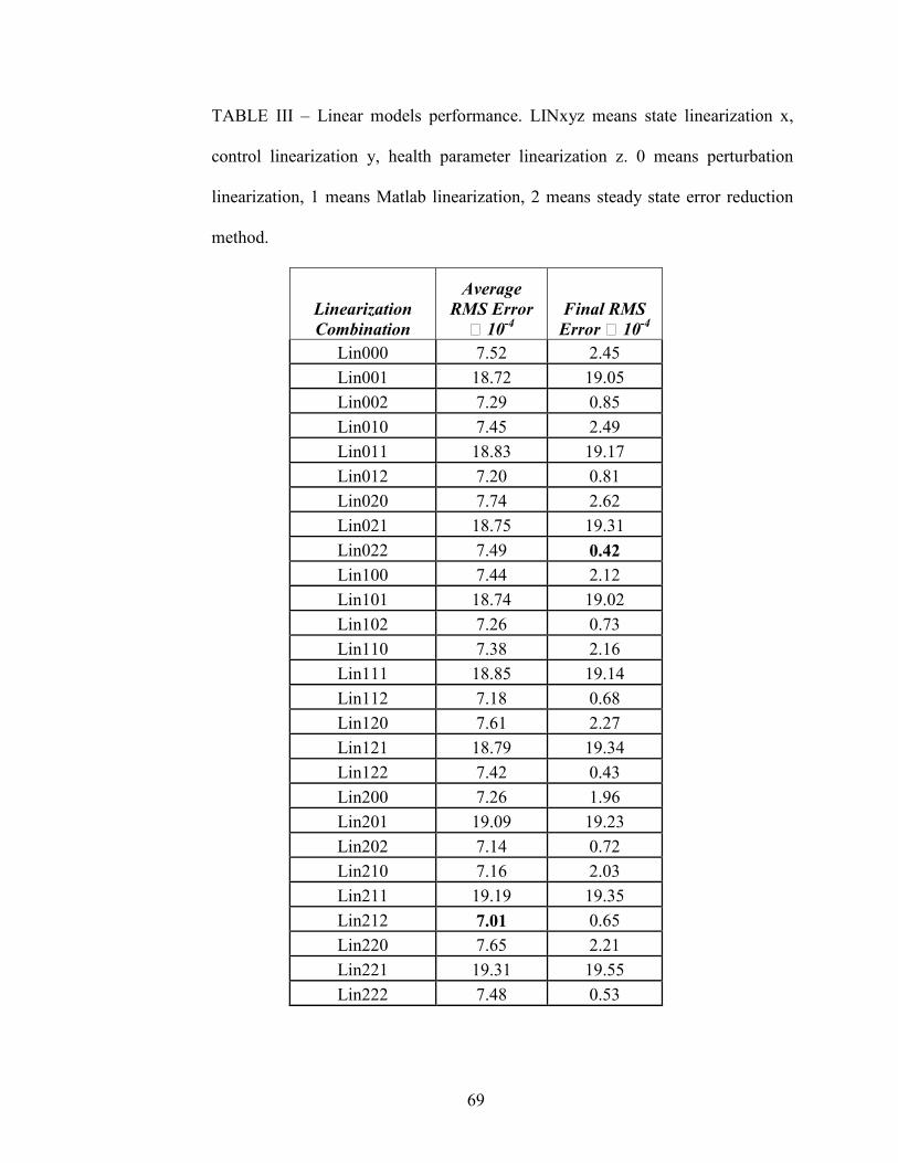
69
TABLE III – Linear models performance. LINxyz means state linearization x,
control linearization y, health parameter linearization z. 0 means perturbation
linearization, 1 means Matlab linearization, 2 means steady state error reduction
method.
Linearization
Combination
Average
RMS Error
� 10-4
Final RMS
Error � 10-4
Lin000 7.52 2.45
Lin001 18.72 19.05
Lin002 7.29 0.85
Lin010 7.45 2.49
Lin011 18.83 19.17
Lin012 7.20 0.81
Lin020 7.74 2.62
Lin021 18.75 19.31
Lin022 7.49 0.42
Lin100 7.44 2.12
Lin101 18.74 19.02
Lin102 7.26 0.73
Lin110 7.38 2.16
Lin111 18.85 19.14
Lin112 7.18 0.68
Lin120 7.61 2.27
Lin121 18.79 19.34
Lin122 7.42 0.43
Lin200 7.26 1.96
Lin201 19.09 19.23
Lin202 7.14 0.72
Lin210 7.16 2.03
Lin211 19.19 19.35
Lin212 7.01 0.65
Lin220 7.65 2.21
Lin221 19.31 19.55
Lin222 7.48 0.53

70
It can be seen that several of the linearization combinations provide performance
nearly as good as the best linearization, but some linearization combinations perform
quite poorly. The linearization technique in which the nonlinear model is linearized with
respect to health parameters in perturbation method or steady state error reduction
method was giving the best RMS errors. From the above results, it can be concluded that
linear models obtained with the perturbation method or steady state error reduction would
behave more close to the nonlinear systems than those obtained with the Matlab method.
5. 2 Health parameter estimation
The turbofan engine’s health parameters are estimated based on some linear model.
The linearized Kalman filter was implemented to estimate all 10 health parameters of the
MAPSS model of the turbofan engine. However, due to an error in the MAPSS software
health parameter # 4 cannot be estimated (i.e., it is completely unobservable, with no
connection to the states or outputs). Two different algorithms were tested for estimating
the health parameters: constrained Kalman filtering and unconstrained (standard) Kalman
filtering.
As discussed in Section 4.4, the discrete linear model of the MAPSS model is
obtained and is then augmented with the health parameters. The Kalman filter works on
the principle of utilizing the known dynamics of the system (model) along with the
measurements obtained from the model to estimate the states. Three seconds of data are
collected at 10 Hz every flight. The model is simulated for 6 seconds so the states reach the
steady state. The necessary measurements were obtained offline using the nonlinear model. The

71
model is linearized every 100 flights but the measurements were obtained every flight
(for 3 sec) from the measurement files.
The list of health parameters that are to be estimated are given as follows.
1) Fan airflow
2) Fan efficiency
3) Booster tip airflow
4) Booster tip efficiency (unobservable in MAPSS)
5) Booster hub airflow
6) Booster hub efficiency
7) High pressure turbine airflow
8) High pressure turbine efficiency
9) Low pressure turbine airflow
10) Low pressure turbine efficiency
The sensor measurements used to estimate the above health parameters are given as
follows with their corresponding SNR (signal-to-noise ratios) values as shown. These
signal-to-noise ratios were determined on the basis of NASA experience and previously
published data [28].
1) LPT exit pressure (SNR = 100)
2) LPT exit temperature (SNR =100)
3) Percent low pressure spool rotor speed (SNR =150)
4) HPC inlet temperature (SNR =100)
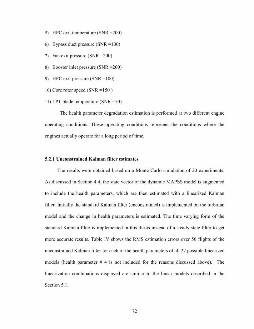
72
5) HPC exit temperature (SNR =200)
6) Bypass duct pressure (SNR =100)
7) Fan exit pressure (SNR =200)
8) Booster inlet pressure (SNR =200)
9) HPC exit pressure (SNR =100)
10) Core rotor speed (SNR =150 )
11) LPT blade temperature (SNR =70)
The health parameter degradation estimation is performed at two different engine
operating conditions. These operating conditions represent the conditions where the
engines actually operate for a long period of time.
5.2.1 Unconstrained Kalman filter estimates
The results were obtained based on a Monte Carlo simulation of 20 experiments.
As discussed in Section 4.4, the state vector of the dynamic MAPSS model is augmented
to include the health parameters, which are then estimated with a linearized Kalman
filter. Initially the standard Kalman filter (unconstrained) is implemented on the turbofan
model and the change in health parameters is estimated. The time varying form of the
standard Kalman filter is implemented in this thesis instead of a steady state filter to get
more accurate results. Table IV shows the RMS estimation errors over 50 flights of the
unconstrained Kalman filter for each of the health parameters of all 27 possible linearized
models (health parameter # 4 is not included for the reasons discussed above). The
linearization combinations displayed are similar to the linear models described in the
Section 5.1.
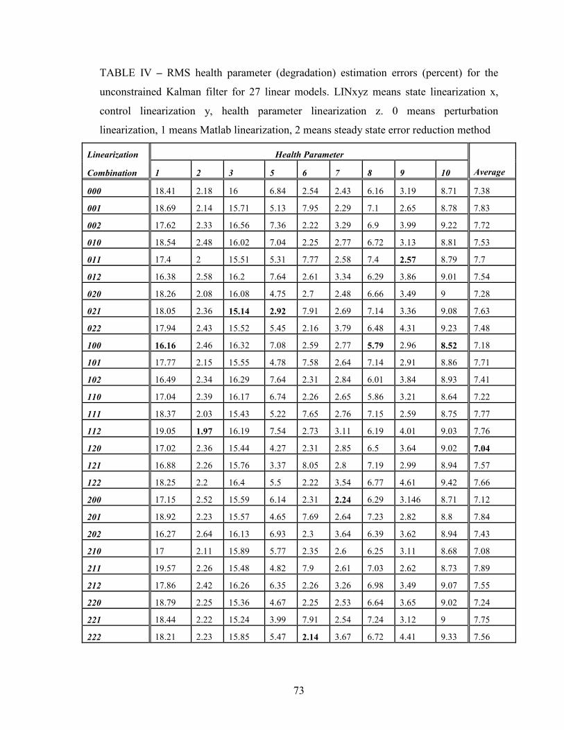
73
TABLE IV – RMS health parameter (degradation) estimation errors (percent) for the
unconstrained Kalman filter for 27 linear models. LINxyz means state linearization x,
control linearization y, health parameter linearization z. 0 means perturbation
linearization, 1 means Matlab linearization, 2 means steady state error reduction method
Linearization Health Parameter
Combination 1 2 3 5 6 7 8 9 10 Average
000 18.41 2.18 16 6.84 2.54 2.43 6.16 3.19 8.71 7.38
001 18.69 2.14 15.71 5.13 7.95 2.29 7.1 2.65 8.78 7.83
002 17.62 2.33 16.56 7.36 2.22 3.29 6.9 3.99 9.22 7.72
010 18.54 2.48 16.02 7.04 2.25 2.77 6.72 3.13 8.81 7.53
011 17.4 2 15.51 5.31 7.77 2.58 7.4 2.57 8.79 7.7
012 16.38 2.58 16.2 7.64 2.61 3.34 6.29 3.86 9.01 7.54
020 18.26 2.08 16.08 4.75 2.7 2.48 6.66 3.49 9 7.28
021 18.05 2.36 15.14 2.92 7.91 2.69 7.14 3.36 9.08 7.63
022 17.94 2.43 15.52 5.45 2.16 3.79 6.48 4.31 9.23 7.48
100 16.16 2.46 16.32 7.08 2.59 2.77 5.79 2.96 8.52 7.18
101 17.77 2.15 15.55 4.78 7.58 2.64 7.14 2.91 8.86 7.71
102 16.49 2.34 16.29 7.64 2.31 2.84 6.01 3.84 8.93 7.41
110 17.04 2.39 16.17 6.74 2.26 2.65 5.86 3.21 8.64 7.22
111 18.37 2.03 15.43 5.22 7.65 2.76 7.15 2.59 8.75 7.77
112 19.05 1.97 16.19 7.54 2.73 3.11 6.19 4.01 9.03 7.76
120 17.02 2.36 15.44 4.27 2.31 2.85 6.5 3.64 9.02 7.04
121 16.88 2.26 15.76 3.37 8.05 2.8 7.19 2.99 8.94 7.57
122 18.25 2.2 16.4 5.5 2.22 3.54 6.77 4.61 9.42 7.66
200 17.15 2.52 15.59 6.14 2.31 2.24 6.29 3.146 8.71 7.12
201 18.92 2.23 15.57 4.65 7.69 2.64 7.23 2.82 8.8 7.84
202 16.27 2.64 16.13 6.93 2.3 3.64 6.39 3.62 8.94 7.43
210 17 2.11 15.89 5.77 2.35 2.6 6.25 3.11 8.68 7.08
211 19.57 2.26 15.48 4.82 7.9 2.61 7.03 2.62 8.73 7.89
212 17.86 2.42 16.26 6.35 2.26 3.26 6.98 3.49 9.07 7.55
220 18.79 2.25 15.36 4.67 2.25 2.53 6.64 3.65 9.02 7.24
221 18.44 2.22 15.24 3.99 7.91 2.54 7.24 3.12 9 7.75
222 18.21 2.23 15.85 5.47 2.14 3.67 6.72 4.41 9.33 7.56
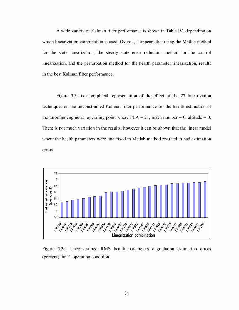
74
A wide variety of Kalman filter performance is shown in Table IV, depending on
which linearization combination is used. Overall, it appears that using the Matlab method
for the state linearization, the steady state error reduction method for the control
linearization, and the perturbation method for the health parameter linearization, results
in the best Kalman filter performance.
Figure 5.3a is a graphical representation of the effect of the 27 linearization
techniques on the unconstrained Kalman filter performance for the health estimation of
the turbofan engine at operating point where PLA = 21, mach number = 0, altitude = 0.
There is not much variation in the results; however it can be shown that the linear model
where the health parameters were linearized in Matlab method resulted in bad estimation
errors.
5.8
6
6.2
6.4
6.6
6.8
7
7.2
Lin120
Lin210
Lin220
Lin110
Lin200
Lin020
Lin100
Lin000
Lin010
Lin102
Lin022
Lin202
Lin222
Lin212
Lin012
Lin122
Lin021
Lin121
Lin112
Lin002
Lin221
Lin011
Lin101
Lin001
Lin111
Lin211
Lin201
Linearization combination
Estimation error
(percent)
Figure 5.3a: Unconstrained RMS health parameters degradation estimation errors
(percent) for 1st operating condition.
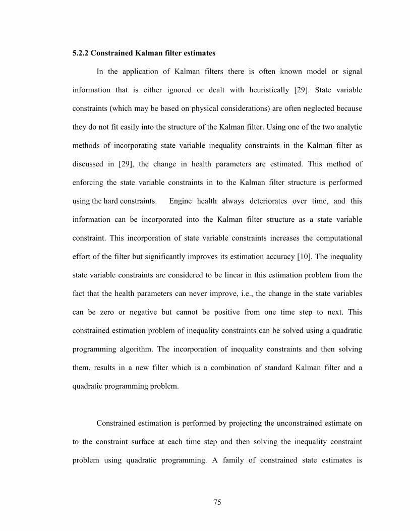
75
5.2.2 Constrained Kalman filter estimates
In the application of Kalman filters there is often known model or signal
information that is either ignored or dealt with heuristically [29]. State variable
constraints (which may be based on physical considerations) are often neglected because
they do not fit easily into the structure of the Kalman filter. Using one of the two analytic
methods of incorporating state variable inequality constraints in the Kalman filter as
discussed in [29], the change in health parameters are estimated. This method of
enforcing the state variable constraints in to the Kalman filter structure is performed
using the hard constraints. Engine health always deteriorates over time, and this
information can be incorporated into the Kalman filter structure as a state variable
constraint. This incorporation of state variable constraints increases the computational
effort of the filter but significantly improves its estimation accuracy [10]. The inequality
state variable constraints are considered to be linear in this estimation problem from the
fact that the health parameters can never improve, i.e., the change in the state variables
can be zero or negative but cannot be positive from one time step to next. This
constrained estimation problem of inequality constraints can be solved using a quadratic
programming algorithm. The incorporation of inequality constraints and then solving
them, results in a new filter which is a combination of standard Kalman filter and a
quadratic programming problem.
Constrained estimation is performed by projecting the unconstrained estimate on
to the constraint surface at each time step and then solving the inequality constraint
problem using quadratic programming. A family of constrained state estimates is
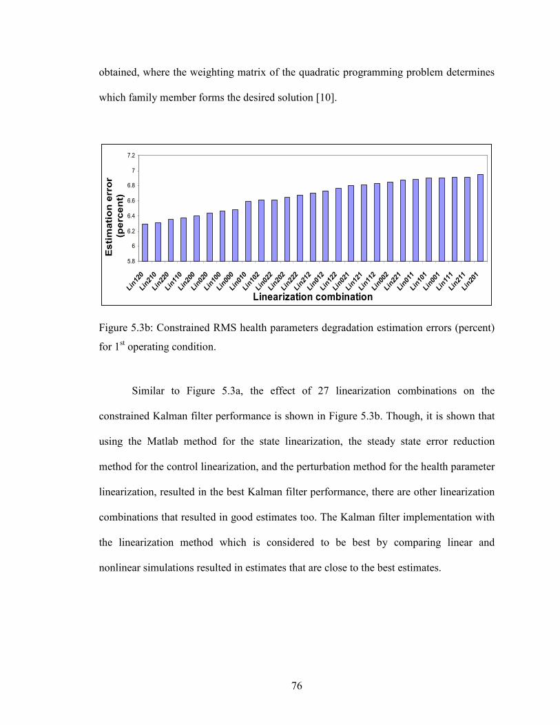
76
obtained, where the weighting matrix of the quadratic programming problem determines
which family member forms the desired solution [10].
5.8
6
6.2
6.4
6.6
6.8
7
7.2
Lin120
Lin210
Lin220
Lin110
Lin200
Lin020
Lin100
Lin000
Lin010
Lin102
Lin022
Lin202
Lin222
Lin212
Lin012
Lin122
Lin021
Lin121
Lin112
Lin002
Lin221
Lin011
Lin101
Lin001
Lin111
Lin211
Lin201
Linearization combination
Estimation error
(percent)
Figure 5.3b: Constrained RMS health parameters degradation estimation errors (percent)
for 1st operating condition.
Similar to Figure 5.3a, the effect of 27 linearization combinations on the
constrained Kalman filter performance is shown in Figure 5.3b. Though, it is shown that
using the Matlab method for the state linearization, the steady state error reduction
method for the control linearization, and the perturbation method for the health parameter
linearization, resulted in the best Kalman filter performance, there are other linearization
combinations that resulted in good estimates too. The Kalman filter implementation with
the linearization method which is considered to be best by comparing linear and
nonlinear simulations resulted in estimates that are close to the best estimates.
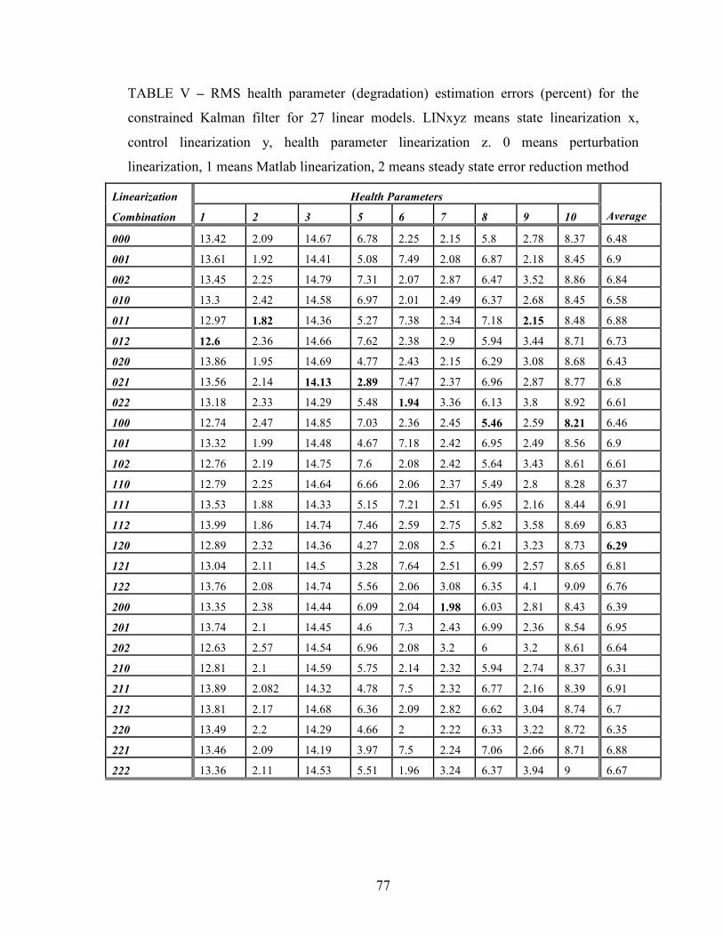
77
TABLE V – RMS health parameter (degradation) estimation errors (percent) for the
constrained Kalman filter for 27 linear models. LINxyz means state linearization x,
control linearization y, health parameter linearization z. 0 means perturbation
linearization, 1 means Matlab linearization, 2 means steady state error reduction method
Linearization Health Parameters
Combination 1 2 3 5 6 7 8 9 10 Average
000 13.42 2.09 14.67 6.78 2.25 2.15 5.8 2.78 8.37 6.48
001 13.61 1.92 14.41 5.08 7.49 2.08 6.87 2.18 8.45 6.9
002 13.45 2.25 14.79 7.31 2.07 2.87 6.47 3.52 8.86 6.84
010 13.3 2.42 14.58 6.97 2.01 2.49 6.37 2.68 8.45 6.58
011 12.97 1.82 14.36 5.27 7.38 2.34 7.18 2.15 8.48 6.88
012 12.6 2.36 14.66 7.62 2.38 2.9 5.94 3.44 8.71 6.73
020 13.86 1.95 14.69 4.77 2.43 2.15 6.29 3.08 8.68 6.43
021 13.56 2.14 14.13 2.89 7.47 2.37 6.96 2.87 8.77 6.8
022 13.18 2.33 14.29 5.48 1.94 3.36 6.13 3.8 8.92 6.61
100 12.74 2.47 14.85 7.03 2.36 2.45 5.46 2.59 8.21 6.46
101 13.32 1.99 14.48 4.67 7.18 2.42 6.95 2.49 8.56 6.9
102 12.76 2.19 14.75 7.6 2.08 2.42 5.64 3.43 8.61 6.61
110 12.79 2.25 14.64 6.66 2.06 2.37 5.49 2.8 8.28 6.37
111 13.53 1.88 14.33 5.15 7.21 2.51 6.95 2.16 8.44 6.91
112 13.99 1.86 14.74 7.46 2.59 2.75 5.82 3.58 8.69 6.83
120 12.89 2.32 14.36 4.27 2.08 2.5 6.21 3.23 8.73 6.29
121 13.04 2.11 14.5 3.28 7.64 2.51 6.99 2.57 8.65 6.81
122 13.76 2.08 14.74 5.56 2.06 3.08 6.35 4.1 9.09 6.76
200 13.35 2.38 14.44 6.09 2.04 1.98 6.03 2.81 8.43 6.39
201 13.74 2.1 14.45 4.6 7.3 2.43 6.99 2.36 8.54 6.95
202 12.63 2.57 14.54 6.96 2.08 3.2 6 3.2 8.61 6.64
210 12.81 2.1 14.59 5.75 2.14 2.32 5.94 2.74 8.37 6.31
211 13.89 2.082 14.32 4.78 7.5 2.32 6.77 2.16 8.39 6.91
212 13.81 2.17 14.68 6.36 2.09 2.82 6.62 3.04 8.74 6.7
220 13.49 2.2 14.29 4.66 2 2.22 6.33 3.22 8.72 6.35
221 13.46 2.09 14.19 3.97 7.5 2.24 7.06 2.66 8.71 6.88
222 13.36 2.11 14.53 5.51 1.96 3.24 6.37 3.94 9 6.67

78
Table V shows the performance of the constrained Kalman filter, depending on
which linearization combination is used. As with the standard Kalman filter, it appears
that using the Matlab method for the state linearization, the steady state error reduction
method for the control linearization, and the perturbation method for the health parameter
linearization, results in the best constrained Kalman filter performance.
Figure 5.3a and 5.3b show that Kalman filter performance is quite bad when the
model is linearized with respect to health parameters in Matlab method. This proves that
Kalman filter performance mainly depends on the linearization accuracy of the nonlinear
model. Hence, accurate estimates can only be obtained by implementing Kalman filter on
the linear models that behave as close as possible to their nonlinear models.
When average health parameter degradation estimation error (percent) is
considered in Tables IV and V, the constrained filter has a smaller estimation error than
the unconstrained filter. This is because the constrained state estimate is unbiased and has
a smaller error covariance than the unconstrained estimate. But this (extra accuracy) is
achieved at the additional computational effort of performing quadratic programming
algorithm at each time step.
Figure 5.4a and 5.4b show the health parameter degradation estimations of
unconstrained filter and constrained filter with the true degradation for 500 flights
respectively. The thick lines show the true degradation of the health parameters and thin
lines represent their corresponding estimations. The true health parameters degradations
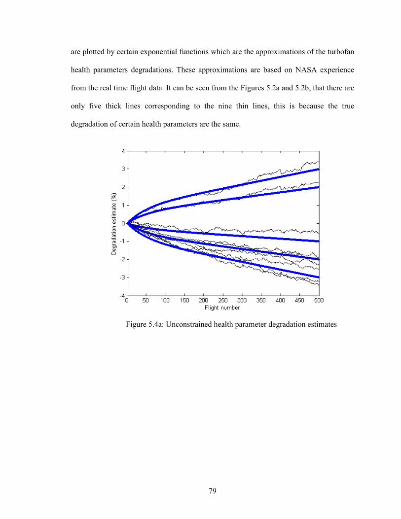
79
are plotted by certain exponential functions which are the approximations of the turbofan
health parameters degradations. These approximations are based on NASA experience
from the real time flight data. It can be seen from the Figures 5.2a and 5.2b, that there are
only five thick lines corresponding to the nine thin lines, this is because the true
degradation of certain health parameters are the same.
Figure 5.4a: Unconstrained health parameter degradation estimates
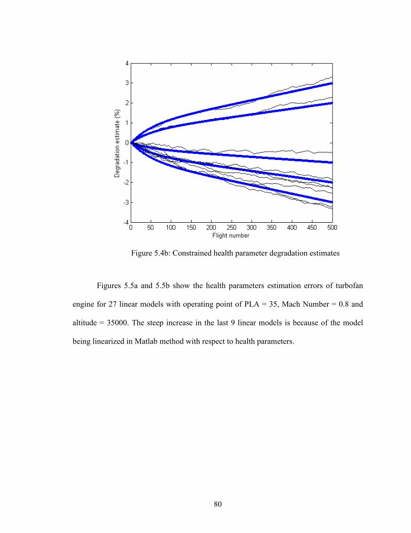
80
Figure 5.4b: Constrained health parameter degradation estimates
Figures 5.5a and 5.5b show the health parameters estimation errors of turbofan
engine for 27 linear models with operating point of PLA = 35, Mach Number = 0.8 and
altitude = 35000. The steep increase in the last 9 linear models is because of the model
being linearized in Matlab method with respect to health parameters.
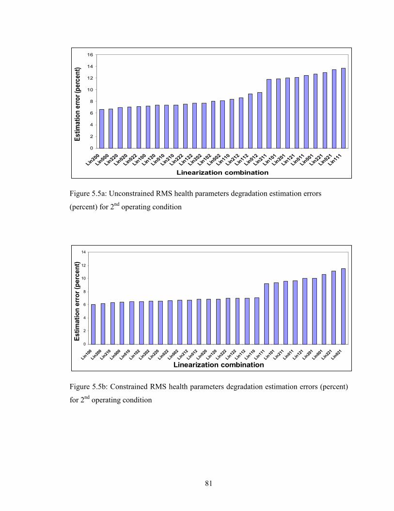
81
0
2
4
6
8
10
12
14
16
Lin200
Lin000
Lin220
Lin020
Lin022
Lin100
Lin120
Lin010
Lin210
Lin222
Lin122
Lin202
Lin102
Lin002
Lin110
Lin212
Lin112
Lin012
Lin211
Lin101
Lin201
Lin121
Lin011
Lin001
Lin221
Lin021
Lin111
Linearization combination
Estimation error (percent)
Figure 5.5a: Unconstrained RMS health parameters degradation estimation errors
(percent) for 2nd operating condition
0
2
4
6
8
10
12
14
Lin100
Lin200
Lin210
Lin000
Lin010
Lin102
Lin202
Lin220
Lin022
Lin002
Lin212
Lin012
Lin020
Lin120
Lin222
Lin122
Lin112
Lin110
Lin111
Lin101
Lin211
Lin011
Lin121
Lin201
Lin001
Lin221
Lin021
Linearization combination
Estimation error (percent)
Figure 5.5b: Constrained RMS health parameters degradation estimation errors (percent)
for 2nd operating condition
82
CHAPTER VI
UNSCENTED KALMAN FILTER
The extended Kalman filter is considered to be the most widely used recursive estimation
algorithm for the nonlinear systems. In this chapter we discuss the major flaws and
assumptions that are encountered in the EKF algorithm and discuss a new estimation
algorithm to overcome those flaws. Years of research in the estimation field has resulted
in many different algorithms which have their own pros and cons. The unscented Kalman
filter is one of those algorithms. This UKF algorithm was first proposed by Julier et
al. [22] and was further developed by Wan and van der Merwe [23]. This UKF is based
on the unscented transformation of the mean and covariance of the parameters to be
estimated.
Estimating the states of a nonlinear system is extremely difficult. The optimal
solution to this estimation requires the propagation of the full PDF (probability density
function) of the states through the time update. This propagation is almost impossible
because the PDF of any variable is not finite (restricted). However, an approximation of
83
some kind is considered for this PDF in estimation algorithms. The Kalman filter uses the
first two moments (mean and covariance) of the state distribution in its update rules.
There are a couple of reasons to consider only mean and covariance. Firstly, the mean
and covariance of the unknown distribution requires the maintenance of a small and
constant amount of information. Secondly, both the mean and covariance are linearly
transformable quantities. For example, if a distribution has the mean M and covariance C,
after the linear transformation T, the mean and covariance will be TM and TCT’.
The EKF basically works on the assumptions that all the transformations are
linear. The EKF is an estimation algorithm wherein the nonlinear system is linearized
first and then the recursive Kalman filter equations are applied for the time update.
Linearizing the nonlinear system involves the calculation of Jacobians and substituting
them for the linear transformation in the KF equations. The EKF is difficult to tune and
may result in unreliable estimates if the nonlinearities are severe. The major limitations of
the EKF are
1) The EKF can be applied only if the Jacobians can be calculated.
2) Jacobian calculation is an extremely difficult and error-prone process.
3) Linearization is based on the Taylor series approximation, considering only the
first two terms of the series and ignoring the other higher order terms.
84
As the EKF totally depends on the linearization to propagate the mean and
covariance, it is obvious that EKF would give bad estimates if any one of the above
limitations is encountered.
To overcome these limitations, the unscented transformation was derived which
utilizes a more direct and simple approach to propagate the mean and covariance. The
main advantage of implementing unscented transformation on a nonlinear estimation
problem is that it approximates the mean to third order, which is better than linearization,
and it approximates the covariance to third order, which is the same as linearization.
Section 6.1 discusses the basic unscented transformation on which UKF was derived. The
UKF algorithm will be derived in Section 6.2. Section 6.3 describes reduced sigma point
filters and finally the performance of the UKF is shown by an inverted pendulum
application in Section 6.4 and its corresponding simulation results in Section 6.5.
6.1 Unscented Transformation
The unscented transformation is a method for calculating the statistics of a
random variable which undergoes a nonlinear transformation [7]. The unscented
transformation is based on two fundamental principles. First, it is easy to perform a
nonlinear transformation on a single point (rather than an entire PDF). Second, it is not
too hard to find a set of points in state space whose probability density function (PDF)
approximates the true PDF of a state vector [24].
85
Consider a random variable x with dimension n which is going through a
nonlinear transformation, y=f(x). Initial condition states that x has a mean x and
covariance xP . The unscented transformation calculates the statistics of y by forming a
set of sigma points (vectors) iX . These sigma points should be chosen such that they
capture the most important statistical properties of the prior random variable x. Sigma
points are calculated according to the following conditions:
0 ,X x=
( ( ) )i x iX x L Pλ= + + i=1,……L,
( ( ) )i x iX x L Pλ= − + i=L+1,……,2L, (6.1)
where 2 ( )L Lλ α κ= + − , is a scaling parameter. The constant α determines the spread of
the sigma points around x which is usually set to a small positive value (0<α <1). κ is a
secondary scaling parameter which is set to 3−L. (set to 0 in our case). ( ( ) )x iL Pλ+ is
the ith column of the matrix square root. This matrix square root can be obtained by using
the Cholesky factorization routine in Matlab.
Each of the sigma vectors is assigned with a weight. These weights are calculated
by the following equations.
( )
0
( ) ( ) 2
0 0
/( )
1
m
c m
W L
W W
λ λ
α β
= +
= + − +
( ) ( ) 1/ 2( )c m
i iW W L λ= = + i=1,……2L (6.2)
86
where β is a factor that incorporates a prior knowledge of the distribution, usually set to
2 (set to 21 α− in our case).
The sigma vectors described in Equation 6.1 are propagated through the nonlinear
function y=f(x) individually and the corresponding iY are obtained as
( )i iY f X= i=0,……, 2L, (6.3)
The mean and covariance of the y are approximated using the above nonlinearly
transformed sigma points ( iY ) and the weights by the following equations.
2( )
0
Lm
i i
i
y W Y=
=∑ (6.4)
2( )
0
( )( )L
c T
y i i i
i
P W Y y Y y=
= − −∑ (6.5)
Hence, y and yP obtained in Equations 6.4 and 6.5 are the approximated mean
and covariance of the nonlinearly transformed x. Figure 6.1 shows how the sigma points
are nonlinearly transformed [22].
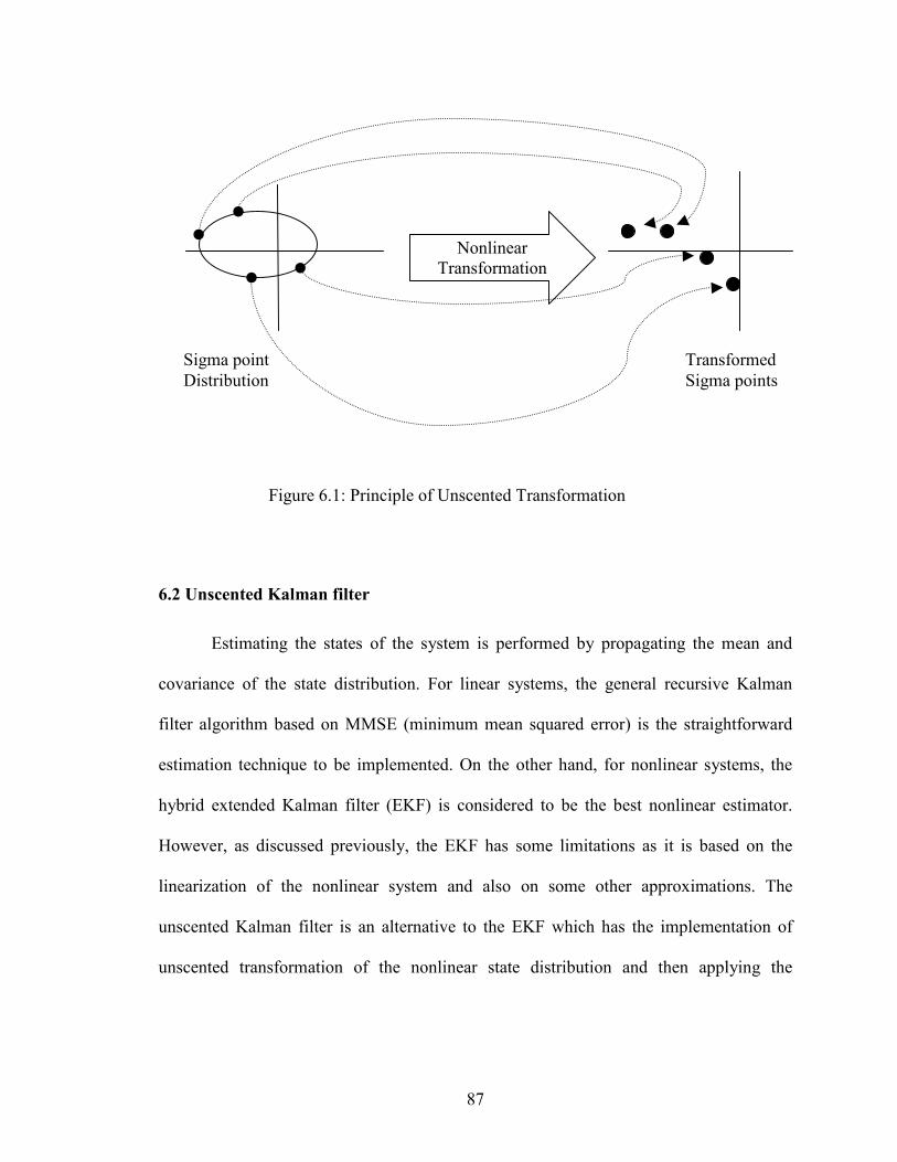
87
Figure 6.1: Principle of Unscented Transformation
6.2 Unscented Kalman filter
Estimating the states of the system is performed by propagating the mean and
covariance of the state distribution. For linear systems, the general recursive Kalman
filter algorithm based on MMSE (minimum mean squared error) is the straightforward
estimation technique to be implemented. On the other hand, for nonlinear systems, the
hybrid extended Kalman filter (EKF) is considered to be the best nonlinear estimator.
However, as discussed previously, the EKF has some limitations as it is based on the
linearization of the nonlinear system and also on some other approximations. The
unscented Kalman filter is an alternative to the EKF which has the implementation of
unscented transformation of the nonlinear state distribution and then applying the
Sigma point
Distribution
Nonlinear
Transformation
Transformed
Sigma points
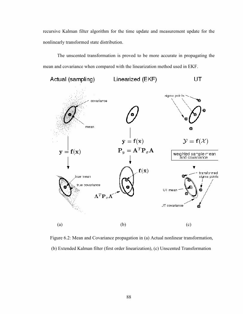
88
recursive Kalman filter algorithm for the time update and measurement update for the
nonlinearly transformed state distribution.
The unscented transformation is proved to be more accurate in propagating the
mean and covariance when compared with the linearization method used in EKF.
(a) (b) (c)
Figure 6.2: Mean and Covariance propagation in (a) Actual nonlinear transformation,
(b) Extended Kalman filter (first order linearization), (c) Unscented Transformation
89
Figure 6.2 illustrates the mean and covariance propagation in all three
transformations [23]. The mean in the EKF and UT are similar to that of the true
nonlinear transformation. But, when covariance propagation is considered, the UT
outperforms the EKF. And moreover there is no need of calculating any Jacobians in the
unscented transformation algorithm. The order of computational effort is almost the same
in both algorithms. When the computational effort is same in both cases, the unscented
transformation is preferred over the EKF for the better accuracy.
The unscented Kalman filter algorithm can be divided in to three sections. The
first part is the initialization of the state estimate and state covariance of the nonlinear
system. The second part is applying the UT to the state distribution and calculating the a
priori state estimate and a priori state covariance. The third part is performing the
measurement update equations and calculating the Kalman gain, state estimate and state
error covariance.
6.2.1 Algorithm for additive noise (zero mean)
Consider a discrete time nonlinear system represented by
1 ( , , )
( , )
k k k k k
k k k k
x f x u t w
y h x t v
+ = +
= + (6.6)
where (0, )k kw N Q� , (0, )k kv N R� are additive process and measurement noise, with
zero mean and covariances of kQ and kR .
Initialization
90
The UKF is initialized with the initial estimate and estimation error covariance as
in the EKF.
0 0
0 0 0 0 0
ˆ ( )
ˆ ˆ[( )( ) ]T
x E x
P E x x x x
+
+ + +
=
= − − (6.7)
Sigma point selection
As seen previously in the unscented transformation, a set of sigma points and their
corresponding weights are calculated around the initial estimate according to Equation
6.1 and 6.2.
( )
1 1ˆ ˆi
k kx x+− −= i=0;
( )
1 1 1ˆ ˆ ( ( ) )i
k k k ix x n Pλ+ +− − −= + + i=1,…, n
( )
1 1 1ˆ ˆ ( ( ) )i
k k k ix x n Pλ+ +− − −= − + i=n+1,…,2n (6.8)
and the corresponding weights are calculated as
( )
0
( ) ( ) 2
0 0
/( )
1
m
c m
W n
W W
λ λ
α β
= +
= + − +
( ) ( ) 1/ 2( )c m
i iW W n λ= = + i=1,…,2n (6.9)
where α , β and λ are as defined in the Section 6.1.
Time Update
91
The system gets updated from k-1 to k time step. All the sigma points ( )
1ˆ i
kx − are
propagated through the nonlinear function f(.) and h(.) and then the corresponding
nonlinear sigma points ( )ˆ ikx are obtained.
( ) ( )
1ˆ ˆ( , , )i i
k k k kx f x u t−=
( ) ( )ˆ ˆ( , )i i
k k ky h x t= (6.10)
Using the ( )ˆ ikx vectors and also the weights ( )c
iW and ( )m
iW we perform the
following steps.
a) the a priori state estimate ˆkx− at time kt is calculated as in Equation 6.4
2( ) ( )
0
ˆ ˆn
m i
k i k
i
x W x−
=
=∑ (6.11)
b) the a priori estimation error covariance
2( ) ( ) ( )
1
0
ˆ ˆ ˆ ˆ( )( )n
c i i T
k i k k k k k
i
P W x x x x Q− − −−
=
= − − +∑ (6.12)
Similarly using the ( )ˆ i
ky vectors (measurements from sigma points) ˆky− is
calculated as
2( ) ( )
0
ˆ ˆn
m i
k i k
i
y W y−
=
=∑ (6.13)
Measurement Update
Using the calculated a priori state estimate, a priori estimation error covariance
and measurement estimate, the following terms are calculated.
92
a) Covariance of the predicted measurement
2( ) ( ) ( )
0
ˆ ˆ ˆ ˆ( )( )n
c i i T
yy i k k k k k
i
P W y y y y R− −
=
= − − +∑ (6.14)
b) Now estimate the cross covariance between ˆkx− and ˆky
− as
2( ) ( ) ( )
0
ˆ ˆ ˆ ˆ( )( )n
c i i T
xy i k k k k
i
P W x x y y− −
=
= − −∑ (6.15)
c) The measurement update of the state estimate and estimate error covariance is
performed using the general Kalman filter equations by calculating the Kalman gain kK
1
k xy yyK P P−=
ˆ ˆ ˆ( )k k k k kx x K y y+ − −= + −
T
k k k yy kP P K P K+ −= − (6.16)
6.2.2 Algorithm for non-additive noise
The equations derived in the above algorithm are for additive noises (process and
measurement noise), but we can implement the same equations with little modification in
case the noises are not additive. Consider a discrete time nonlinear system represented by
the following equations.
1 ( , , , )
( , , )
k k k k k
k k k k
x f x u w t
y h x v t
+ =
= (6.17)
93
kw and kv are the process and measurement noises respectively, which are incorporated
in to the system and are clearly non additive.
The modifications that are to be made in the above algorithm are:
a) Augment the noise vectors onto the state vector
k
a
k k
k
x
x w
v
=
(6.18)
b) The UKF is used to estimate the augmented state a
kx . For this we need different initial
conditions from that of the above derived algorithm.
0( )
ˆ 0
0
a
k
E x
x +
=
0 0 0 0
0 0
0
ˆ ˆ[( )( ) ] 0 0
0 0
0 0
T
a
E x x x x
P Q
R
+
− −
=
(6.19)
where 0x , 0Q and 0R have the same value as in the previous case.
c) As the UKF estimates the augmented state (both state and noise) instead of only the
state vector, the 1kQ − term in Equation 6.12 and kR in Equation 6.14 are removed from
the algorithm.
Once these modifications are made, the UKF can be implemented recursively to
estimate the state and the covariance.

94
6.3 Sigma point selection analysis
Sigma points are a set of deterministically chosen points which match the mean
and covariance of a probability distribution (not necessarily Gaussian). Sigma points are
calculated by the square root decomposition of the estimation error covariance. These are
distributed on either side of the state estimate with a value of factor of the square root of
the estimation error covariance. In the previously discussed algorithm a total of 2n+1
sigma points are used. Then, all of the 2n+1 sigma points are propagated through the
nonlinear function (system) to calculate the weighted mean and covariance which in turn
approximate the state estimate and error covariance. It is obvious from the above
discussion that at each time step, a set of 2n+1 sigma points are propagated through the
nonlinear function. On the other hand, in the EKF the system has to be linearized at each
time step to estimate the state and error covariance.
The main computational effort in the UKF is the number of sigma points to be
used for the estimation. So it has become very difficult computationally to estimate the
states of a higher order system using the UKF. Lots of research is going on in this
particular field to reduce the number of sigma points and achieve the same amount of
accuracy as with the 2n+1 sigma points. This research has resulted in the following sets
of sigma points.
a) The simplex sigma point set [25]
b) The minimal skew simplex sigma point set [26]
95
c) The simplex spherical sigma point set [27]
6.3.1 Algorithm for minimal skew simplex sigma point set
It is stated in [25] that given only an n-dimensional mean and covariance estimate,
with no other error distribution information, a set of n+1 sigma points can be constructed
that fully captures all of the known statistics of the error distribution, i.e., its mean and
covariance. This is set is called the simplex sigma point set. This is the only set of all
possible sets of sigma points which match the statistics of the distribution (mean and
covariance) to second order.
However, many filtering and control applications involve the use of a measuring
process that introduces errors that can be empirically characterized to some extent. This
characterization represents the information regarding the higher moments of distribution
like skew (third order moment) and kurtosis (fourth order moment). But, the simplex
sigma point set of n+1 points does not incorporate the information about these higher
order moments. So to overcome this difficulty, a new set of sigma points called the
minimal skew simplex sigma point set has been derived to incorporate the information
about the third order moment and also to minimize its value. An additional sigma point
at the origin transforms the simplex sigma point set to the minimal skew simplex sigma
point set. The sigma point selection algorithm for the minima skew simplex sigma point
set is as follows.
96
1) Chose 00 1W≤ ≤
2) Choose the weight sequence:
0(1 ) / 2niW W= − i=1
1iW W= i=2
2
12iiW W−= i=3,……,n+1 (6.20)
3) Initialize the vector sequence
1
0 [0]X = , 1
1 1[ 1/ 2 ]X W= − and 1
2 1[1/ 2 ]X W= (6.21)
4) Expand the vector sequence for j=2,……,n according to the following equations
1 0
0
j
j
i
XX +
=
i=0
1
11/ 2
j
ij
i
j
XX
W
+
+
=
− i=1,……,j
1
1
0
1/ 2
jj
i
j
XW
+
+
=
i=j+1 (6.22)
where 0 j represents a zero vector of size jx1.
97
The estimation accuracy with the minimal simplex sigma point set is the same as
with the general symmetric sigma point set of 2n+1 points but with half the
computational cost. According to the above algorithm sigma point selection would result
in all the sigma points placed on a sphere around the origin (zero-th point) with a radius
equal to their corresponding weights [26]. The weights on each point vary by a factor of
2n and the values on the coordinates of each point vary by a factor of / 22n . This weight
assignment and value assignment to sigma points would lead to big numerical problems
for higher order systems (very high n). To overcome this difficulty, a new set of points
which have better behavior at higher dimensions was derived.
The new set of points is called the spherical simplex sigma point set [27]. In this
set all sigma points lie on origin or on a hypersphere centered at the origin. The following
section describes the spherical simplex sigma point set.
6.3.2 Algorithm for spherical simplex sigma point set
1) Choose 00 1W≤ ≤
2) Choose the weight sequence:
0(1 ) /( 1)iW W n= − + (6.23)
3) Initialize the vector sequence as:
1
0 [0]X = , 1
1 1[ 1/ 2 ]X W= − and 1
2 1[1/ 2 ]X W= (6.24)
4) Expand the vector sequence for j=2,……, n according to the following equations.
1
0
0
j
j
i
XX
− =
i=0
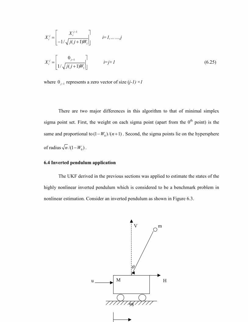
98
1
11/ ( 1)
j
ij
i
XX
j j W
− =
− + i=1,……,j
1
1
0
1/ ( 1)
jj
iXj j W
− =
+ i=j+1 (6.25)
where 10 j− represents a zero vector of size (j-1) ×1
There are two major differences in this algorithm to that of minimal simplex
sigma point set. First, the weight on each sigma point (apart from the 0th point) is the
same and proportional to 0(1 ) /( 1)W n− + . Second, the sigma points lie on the hypersphere
of radius 0/(1 )n W− .
6.4 Inverted pendulum application
The UKF derived in the previous sections was applied to estimate the states of the
highly nonlinear inverted pendulum which is considered to be a benchmark problem in
nonlinear estimation. Consider an inverted pendulum as shown in Figure 6.3.
V m
θ
u H M
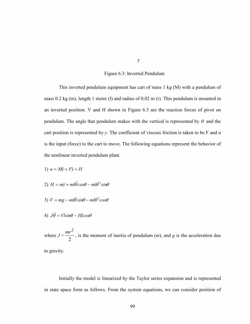
99
y
Figure 6.3: Inverted Pendulum
This inverted pendulum equipment has cart of mass 1 kg (M) with a pendulum of
mass 0.2 kg (m), length 1 meter (l) and radius of 0.02 m (r). This pendulum is mounted in
an inverted position. V and H shown in Figure 6.3 are the reaction forces of pivot on
pendulum. The angle that pendulum makes with the vertical is represented by θ and the
cart position is represented by y. The coefficient of viscous friction is taken to be F and u
is the input (force) to the cart to move. The following equations represent the behavior of
the nonlinear inverted pendulum plant.
1) u My Fy H= + +&& &
2) 2H my ml cos ml sinθ θ θ θ= + −&& &&&
3) 2V mg ml sin ml cosθ θ θ θ= − −&& &
4) J Vlsin Hlcosθ θ θ= −&&
where J =
2
2
mr, is the moment of inertia of pendulum (m), and g is the acceleration due
to gravity.
Initially the model is linearized by the Taylor series expansion and is represented
in state space form as follows. From the system equations, we can consider position of
100
the cart (y), velocity of the cart ( y& ), angle of the pendulum with the vertical (θ ) and
angular displacement (θ& ) to be four states of the system that are to be estimated. The
control input (u) is considered to be a function of angleθ . It is also assumed that the
position of the cart can be measured, i.e., y is the measurement obtained from the system.
x Ax Bu= +& (6.26a)
y Cx Du= + (6.26b)
where
0 1 0 0
0 - / - / 0
0 0 0 1
0 / / ( ) / / 0
F M mg MA
F M l M m g M l
=
+
,
0
1/
0
-1/
MB
Ml
=
, [ ]1 0 0 0C =
and D = 0 since there is no effect of the control on the measurements.
The system is run in open loop with an initial angle of 0.1 radians for 3 sec with a
time step of 0.005 sec. The nonlinear simulations are run to plot the true states of the
systems. Then the extended Kalman filter and unscented Kalman filter algorithms are
implemented to estimate the states of the inverted pendulum. The extended Kalman filter
estimates the states using the above calculated Jacobians for the linearization. But the
unscented Kalman filter is implemented by running the nonlinear model with the
calculated sigma points.
The extended Kalman filter is implemented by calculating the linearized model at
every time step. Linearizing the inverted pendulum model at every time step may not
101
seem to be a big computational effort because they are just four second-order differential
equations to be solved, but for a bigger problem like MAPSS it is really cumbersome. On
the other hand, the unscented Kalman filter estimates the states by propagating a set of
sigma points through the nonlinear system at every time step. There will be 9 sigma
points to be propagated at each time step as discussed in Section 6.2 (2n+1 sigma points
for an nth order system). Similar to the computational effort discussed for the extended
Kalman filter, propagating the sigma points through huge systems can be a problem.
Implementation of the unscented Kalman filter for MAPSS model is discussed in more
detail in Chapter VII.
6.5 Simulation results
Figure 6.4a and 6.4b show the state estimations of the extended Kalman filter and
unscented Kalman filter along with the true states over the entire simulation time.
Considering the first state from Figure 6.4a, the position of the cart, we can conclude that
both estimation techniques were equally good. The reason behind that accuracy is that it
was the only state that could be measured. When velocity estimation is considered, it can
be seen that the unscented Kalman filter was performing better than the extended Kalman
filter after a time of 1.5 seconds. And finally the plots in Figure 6.4b, the last two states
estimations, show that the unscented Kalman filter was far better than the extended
Kalman filter as time increases. It can be seen that the unscented Kalman filter was
tracking the true state over the entire time, but the extended Kalman filter was unable to
track the true state after a certain time. The main reason behind the unscented Kalman
filter performing better than the extended Kalman filter is that the unscented
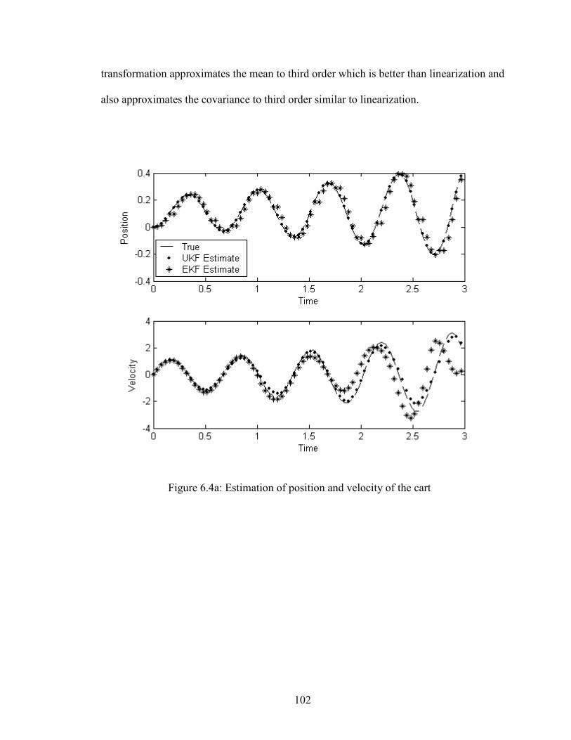
102
transformation approximates the mean to third order which is better than linearization and
also approximates the covariance to third order similar to linearization.
Figure 6.4a: Estimation of position and velocity of the cart
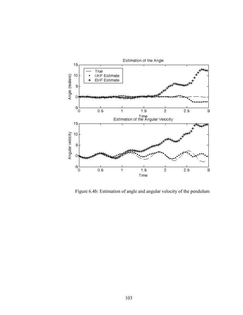
103
Figure 6.4b: Estimation of angle and angular velocity of the pendulum

104
CHAPTER VII
CONCLUSIONS AND FUTURE WORK
7.1 Conclusions
The performance of the 27 linearization combinations was investigated.
Comparisons were made on the basis of RMS difference between linear and nonlinear
models over an entire six-second simulation, RMS difference at the final time of the
simulation, and RMS parameter estimation error of a Kalman filter.
When RMS difference (averaged over the entire simulation) between the linear
and nonlinear models is considered, the best linearization method is
(1) Steady state error reduction method for state linearization
(2) Matlab method for control linearization.
(3) Steady state error reduction method for health parameter linearization
When RMS difference (at the final time) between the linear and nonlinear models
is considered, the best linearization method is
105
(1) Perturbation method for state linearization
(2) Steady state error reduction method for control linearization.
(3) Steady state error reduction method for health parameter linearization
When Kalman filtering health parameter estimation for the engine operating at
ground condition, i.e., first operating condition (with PLA=21, Mach number=0 and
altitude=0) is considered, the best linearization method is
(1) Matlab method for state linearization
(2) Steady state error reduction method for control linearization
(3) Perturbation method for health parameter linearization.
When the engine is operated at cruise, i.e., second operating condition (with
PLA=35, Mach number=0.8 and altitude=35000) is considered, then best linearization
method is
(1) Steady state error reduction method for state linearization
(2) Perturbation method for control linearization
(3) Perturbation method for health parameter linearization.
The linearization combinations mentioned above are considered to be best, but
there are other combinations that behaved close to the best. One important conclusion
that can be made is that linearizing the nonlinear model in Matlab method gives worst
results.
106
7.2 Future work
Further work could involve more investigations of the effect of linearization on
Kalman filtering. This thesis presents the effects only on the first 50 flights. An entire
500-flight investigation may be useful, although the computational effort would be a
consideration. We would have to perform 20 Monte Carlo runs of 27 linearization
combinations of 500 flights each, once for the unconstrained filter and once for the
constrained filter. To be complete we could check three different perturbation amounts
for each of the linearization methods. This gives a total of (20 × 27 × 27 × 2) Kalman
filter simulations.
Other work for the future could involve reproducing these results for other
filtering techniques, such as unscented Kalman filtering or H-infinity filtering. As
discussed in Chapter V, the unscented Kalman filter works on the principle of the
unscented transformation. It has its own advantages and disadvantages. Linearization of
the MAPSS model, the main computational task in linearized Kalman filter estimation
technique, can be overcome (reduced) by applying the unscented Kalman filter to
MAPSS model. However, the unscented Kalman filter is still more computationally
expensive because of the simulations required for state estimate propagation.
Implementing the unscented Kalman filter on MAPSS is not that easy
computationally, as it would be required to run the nonlinear model at every time step for
27 times (since 2n+1 sigma points are propagated through the nonlinear model where n is
the number of augmented states to estimated). The nonlinear MAPSS model is simulated
107
for 6 seconds and the time step considered in estimating the health parameters was 0.1
seconds. This implies that there would be 30 time steps for estimating the health
parameters for each flight as the time for one flight is considered to be 3 seconds. So, that
would take 30 × 27 MAPSS simulations for estimating the health parameter degradation
after one flight. Hence, this is cumbersome to implement computationally. But this
should give results that are better than what linearized Kalman filter achieved. The
unscented Kalman filter was shown to be working better than the extended Kalman filter
for a small state problem (inverted pendulum) in Chapter V.
A MAPSS simulation for 6 seconds would take around 42 seconds of CPU time
on a Pentium-IV, 1.8 GHz, 256 MB RAM system. This would take around 472.5 (30 ×
27 × 50 × 42 / 3600) hours of CPU time to estimate the health parameter of the turbofan
engine for 50 flights. On the other hand, reducing the time step for the estimation of
health parameters would result in small numbers to implement the unscented Kalman
filter. But, the estimates may not be as good as those obtained with 0.1 second time steps.
So, there is a tradeoff to be considered while estimating the states with an unscented
Kalman filter for bigger models (large state problems).
Finally, the results obtained with the unscented Kalman filter after the time step
reduction should be compared with those obtained with the linearized Kalman filter with
similar time step. This would really lead us to decide if the unscented Kalman filter is
better than the linearized or extended Kalman filters.

108
BIBLIOGRAPHY
[1] Santanu Chatterjee and Jonathan Litt, “Online model parameter estimation of jet
engine degradation for autonomous propulsion control,” NASA TM 2003-
212608.
[2] D. Doel, “An assessment of weighted-least-squares-based gas path analysis,”
ASME Journal of Engineering for Gas Turbines and Power (116) pp. 366-373,
April 1994.
[3] H. DePold and F. Gass, “The application of expert systems and neural networks to
gas turbine prognostics and diagnostics,” ASME Journal of Engineering for Gas
Turbines and Power (232) pp. 607-61, Oct. 1999.
[4] A. Volponi, H. DePold, and R. Ganguli, “The use of Kalman filter and neural
network methodologies in gas turbine performance diagnostics: a comparative
study,” Proceedings of ASME TurboExpo 2000, pp. 1-9, May 2000.
[5] T. Kobayashi and Donald L. Simon, “A hybrid neural network-genetic algorithm
technique for aircraft engine performance diagnostics,” 37th AIAA/ ASME/ SAE/
ASEE Joint Propulsion Conference, July 2001.
[6] Khary I. Parker and Ten-Heui Guo, “Development of a Turbofan Engine
Simulation in a Graphical Simulation Environment,” NASA TM 2003-212543.
[7] Simon J. Julier and J.K.Uhlmann, “A new extension of the Kalman filter to
nonlinear systems,” Proceedings of AeroSense: The 11th international symposium
on Aerospace/Defense Sensing, Simulation and controls, 1997.
109
[8] The aircraft gas turbine engine and its operation, United Technologies
Corporation, August 1988.
[9] Mark Burleigh, Improvements in aero engine design in the last 50 years,
http://students.bath.ac.uk/en2mdb/ass-tj.htm
[10] Dan J. Simon and Donald L. Simon, “Aircraft Turbofan Engine Health Estimation
Using Constrained Kalman Filtering,” 2003, ASME IGTI Turbo Expo, Atlanta,
June 16-19, 2003.
[11] Khary I. Parker and Kevin J. Melcher, “Modular Aero Propulsion System
Simulation (MAPSS) User’s Guide,” NASA TM 2004-212968.
[12] MATLAB, “Getting Started with MATLAB,” The Math Works, Inc., 1996
[13] Simulink, “Using Simulink,” The Math Works Inc., 2000
[14] Panos J. Antsaklis and Anthony N. Michel, “Linear Systems, ” The McGraw-Hill
Companies, Inc., 1997
[15] Arthur Gelb, “Applied optimal estimation,” The M.I.T press, 1974.
[16] Robert Stengel, “Optimal control and estimation,” Dover Publications, New York,
1994.
[17] Kalman R.E., “A New Approach to Linear Filtering and Prediction Problems,”
Journal of Basic Engineering (ASME), vol. 82D, pp. 35-45, March 1960.
[18] Dan J. Simon, Fundamentals of Kalman Filters,
http://academic.csuohio.edu/simond/courses/kalman/
[19] S. Kosanam and D. Simon, “Kalman Filtering with Uncertain Noise
Covariances,” Intelligent Systems and Control, Honolulu, HI, pp. 375-379,
August 2004.
110
[20] John S. Bay, “Fundamentals of Linear State Space Systems,” WCB/ McGraw-Hill
Publications, 1999.
[21] B. Anderson and J. Moore, “Optimal Filtering,” Prentice Hall, 1979
[22] Simon J. Julier and J.K.Uhlmann, “Unscented Filtering and Nonlinear
Estimation,” Proceedings of the IEEE, vol.92, no.3, pp. 401-422, March 2004.
[23] E.A. Wan and R.V.Merwe, “The unscented Kalman filter,” in Kalman Filtering
and Neural Networks (S. Haykin, ed.), John Wiley & Sons, Inc., 2001.
[24] Dan J. Simon, “The unscented Kalman filter,” unpublished notes, 2004.
[25] Simon J. Julier and J.K.Uhlmann, “Reduced sigma point filters for the
propagation of means and covariances through nonlinear transformations,”
Proceedings of American Control Conference, vol. 2, pp. 887-892, 2002.
[26] Simon J. Julier, “The scaled unscented transformation,” Proceedings of American
Control Conference, Anchorage, AK, pp. 4555 - 4559, May 8-10, 2002.
[27] Simon J. Julier, “The spherical simplex unscented transformation,” Proceedings
of American Control Conference, Denver, Colorado, pp.2430-2434, June 4-6,
2003.
[28] W. Merrill, “Identification of multivariable high-performance turbofan engine
dynamics from closed-loop data,” AIAA Journal of Guidance, Control and
Dynamics (7)6 pp. 677-683, Nov. 1984
[29] Dan J. Simon and Donald L. Simon, “Kalman filtering with inequality constraints
for turbofan engine health estimation”, submitted for publication.

111
[30] S. Kosanam, Kalman Filter for Uncertain Noise Covariances, Cleveland State
University, Department of Electrical and Computer Engineering, Masters Thesis,
2004.