LINEAR TRANSIENT FLOW SOLUTION Department …gaia.pge.utexas.edu/papers/infill.pdf · LINEAR...

LINEAR TRANSIENT FLOW SOLUTIONFOR PRIMARY OIL RECOVERY

WITH INFILL AND CONVERSION TO WATER INJECTION

Eric Zwahlen and Tad W. PatzekU.C. Oil Consortium

Department of Materials Science and Mineral Engineering591 Evans Hall, University of California at Berkeley

Berkeley, CA 94720

ABSTRACT

In this paper, we analyze the effects of primary production, producer infills andrepressurization by water injection in a low-permeability, compressible, layeredreservoir filled with oil, water and gas. The sample calculations are for theCalifornia Diatomites, but the equations apply to other tight rock systems. Primaryoil recovery from rows of hydrofractured wells is described by linear transientflow of oil, water and gas with the concomitant pressure decline. During primary,it may be desirable to drill infill wells to accelerate oil production. At some latertime, the infill wells may be converted into waterflood injectors for pressuresupport and incremental oil recovery. We analyze the pressure response and fluidflow rates for the original wells and infill wells drilled halfway between theoriginal wells, and - finally - from water injection at the infill wells. All of theformation and fluid properties are described by a single hydraulic diffusivityassumed to be independent of time and production or injection. We solve the one-dimensional pressure diffusion equation analytically using pressure boundaryconditions at the original and infill wells and use superposition to account for thewater injection. We give solutions for the pressure in the formation, oil, water andgas rates and cumulatives at both the original wells and infill wells as functions oftime. Finally, we present a computational example of oil production from a stackof seven independent diatomite layers with different properties and show theeffects of infill wells and water injection on the total oil production. We show thata single-layer analytical solution and a 1-D numerical simulation for primaryproduction in the diatomite agree well. Our analysis can predict the onset ofpressure depletion and quantify how long to produce from the infill wells beforeinjecting water. We show that producing from the infill well for a few yearssignificantly increases the production from the field and can minimize the lostproduction at the infill well because of conversion to a waterflood injector.

INTRODUCTION

The late and middle Miocene diatomaceous oil fields in the San Joaquin

Valley, California, are located in Kern County, some 40 miles west of Bakersfield.

The largest oil volumes are found in the South, Middle and North Belridge

Diatomite and Brown Shale, Lost Hills Diatomite and Brown Shale, Antelope

Hills, McDonald Anticline, Chico-Martinez Chert, Cymric Diatomite, McKittrick,

Railroad Gap, Belgian Anticline, Asphalto, Elk Hills, Buena Vista Antelope

Shale, and Midway Sunset Reef Ridge and Antelope Shale. An estimated original

oil in place (OOIP) in the Monterey diatomaceous fields exceeds 10 billion barrels

and is comparable to that in Prudoe Bay in Alaska.

Cyclic bedding of the diatomite1 is a well-documented phenomenon, attributed

to alternating deposition of detritus beds, clay, and biogenic beds. The cycles span

length scales that range from a fraction of an inch to tens of feet, reflecting the

duration of depositional phases from semiannual to thousands of years. On a large

scale, there are at least seven distinct oil producing layers with good lateral

continuity within each layer, but little vertical continuity between adjacent layers.

The diatomites are very porous (25 to 65 percent), rich in oil (35 to 70 percent),

and nearly impermeable (0.1 to 10 millidarcies). The high porosity and oil

saturation, together with large thickness (up to 1000 feet) and area (up to a few

square miles per field) translate into the gigantic OOIP estimates.

To compensate for the low reservoir permeability, all wells in the diatomite

must be hydrofractured. A typical well has 3 to 8 fractures with an average

fracture half-length of 150 feet. Wells are usually spaced along lines following

the maximum in-situ stress every 330 feet (2-1/2-acre), 165 feet (1-1/4-acre) or

even 82 feet (5/8-acre). Thousands of hydrofractures have been already induced

and thousands more may be created as new recovery processes, such as

waterflood,2-4 or steam drive 5,6 on 5/8 acre spacing, become commercially viable.

Primary oil production on 2-1/2-acre spacing, followed by infill to 1-1/4 acre

and subsequent conversion to waterflood is of great interest to the producers of

the diatomaceous oil fields. We start from the mathematical formulation of the

problem. We then present a computational example of a seven-layer diatomite

reservoir. We also compare a single-layer analytical solution for primary

production with a 1-D reservoir simulation. In Appendix A, we list several

correlations of PVT properties of oil and solution gas.

PROBLEM STATEMENT

In a compressible, homogeneous porous medium, the pressure distribution

follows a simple diffusion equation. With suitable boundary conditions and an

initial condition, the pressure and fluid velocity in the medium can be calculated

analytically. In this paper, we analyze a reservoir at some uniform initial pressure

pi at t = 0. First, we drill a series of wells with spacing 2L and wellbore flowing

pressure pwell . All wells are hydrofractured, and all of the fractures are rectangular

and have permeabilities that are much higher than the formation permeability.

Therefore, we can assume that the uniform pressure pwell is imposed throughout

the entire hydrofracture. Second, at some time tinf , we drill infill wells halfway

between the original wells and also produce these wells at pwell . Third, at time tinj ,

we inject water into the infill wells at the downhole injection pressure pinj and

continue producing at the original wells. This final step is to quantify the effect of

repressurization of the formation.

This statement of primary production, followed by infill and injection, is a

simplification of what actually occurs. Here we assume uniform and constant

properties in each layer and constant pressures in the wells, and we neglect the

effect production and injection may have on fluid and rock properties. We assume

each of the layers in the reservoir is independent, solve the problem for each layer

separately, and add the individual layer solutions. These assumptions allow us to

derive an analytical solution that can show us the effect of each of the system

parameters on the production.

Original Primary Production

The one-dimensional pressure diffusion equation is

∂∂

α ∂∂

p

t

p

xx L t= ≤ ≤ >

2

2 0 0, , (1)

where

a lf

= t

tc(2)

is the hydraulic diffusivity, which accounts for the total compressibility of the

formation, ct , and the total fluid mobility, λ t . All of the formation and fluid

properties are combined into the single constant parameter α (see Appendix A).

As mentioned, we assume α remains constant during production and injection.

From symmetry we write the equations only for 0 ≤ ≤x L , where the original

wells are at x L= ± . The initial condition is uniform pressure everywhere in the

layer,

p x p x Li( , ) , .0 0= ≤ ≤ (3)

The boundary conditions for primary production are

∂∂p

xt

p L t p

t t

well

inf

0 0,

,,

a fa f

=

=

UV|W|

< (4)

Before the infill time, the symmetry halfway between the original wells at x = 0

requires a no-flow boundary condition, which is specified by the gradient of the

pressure being equal to zero. The pressure at the primary production well at x L=

is specified as the well flowing pressure.

This system of equations can be solved by separation of variables.7 The zero-

gradient condition at x = 0 leads to a cosine expansion of the initial condition.

The pressure before infill is

p x t p p px L

e x L t twell i welln n

n

t L

ninf

n, ( )cos /

, ,/a f b g b g= + − − ≤ ≤ < <−

=

∞

∑2 1 0 02 2

0

λλ

λ α

(5)

where

l pn n n= + =2 1

20 1 20 5 , , , , K (6)

This cosine series clearly shows that the boundary conditions before the infill time

are satisfied. The time dependence of the pressure is controlled by α divided by

L2 .

An alternate form of the solution, obtained most easily by Laplace Transform,

is better suited for early times7:

p x t p p pn x L

t L

n x L

t L

x L t t

well i welln

n

inf

,/

/

/

/

,

a f b g a f a f a f= + − − − + − + + +RSTUVW

LNMM

OQPP

≤ ≤ >=

∞

∑1 12 1

2

2 1

2

0

2 20

erfc erfcα α (7)

We can obtain the average pressure p in the reservoir by integrating the

pressure profile from x = 0 to x L= and then dividing by L:

p tL

p x t dxL

( ) ( , )= ′ ′z1

0

(8)

Alternatively we can consider a “pressure” balance on the system. This is

actually an energy balance where the energy density is p L/ . Then the average

pressure is the initial uniform pressure minus the “lost” pressure that has flowed

out the boundary:

p t pL

p

xdti

x L

t

( ) = − −FHG

IKJ ′

=z1

0

α ∂∂

(9)

Inserting the pressure distribution given in (5) into (8) gives the average

pressure on primary as

p p p pe

well i well

t L

nn

n

= + −−

=

∞

∑22 2

20

b gλ α

λ

/

(10)

The average pressure from the complimentary error function solution is most

easily obtained using (9). Then the average pressure is

p p p p t Ln

t Li i well

n

n

= − − + −FHG

IKJ

RS|T|

UV|W|=

∞

∑21

2 12

21

b g απ α

/ ( )/

ierfc (11)

where

ierfc erfcz e z zz0 5 0 5= −−1 2

π(12)

The ierfc function is negligible for large arguments (early times), so this equation

clearly shows that the average pressure initially drops linearly with the square root

of time.

Primary After Infill

At the infill time, an infill well is drilled at x = 0, and the pressure is specified

at both boundaries of the system. This set of boundary conditions leads to a sine

series expansion of the original cosine series. We set t t= inf in (5) and use the

result as the initial condition for a new set of side conditions to solve (1). The

initial condition is

p x t p p px L

e x Linf well i welln n

n

t L

n

n inf, ( )cos /

,/c h b g b g= + − − ≤ ≤−

=

∞

∑2 1 02 2

0

λλ

λ α(13)

The boundary conditions are specified as constant-pressure conditions by

p t p

p L t pt t

well

well

inf

0,

,,

a fa f

=

=UVW

≥ (14)

Again by separation of variables, the solution to (1) is given by

p x t p p px

Le

e

x L t t

well i well mm

m

t t Ln t L

n m nn

inf

m inf

n inf

, sin( )

,

,

//

a f b g c hd i= + − F

HGIKJ

−−

≤ ≤ >=

∞− −

−

=

∞

∑ ∑41

0

12 2

0

2 2

2 2

β βλ β λ

β αλ α

(15)

where

b pm m m= =, , , ,1 2 3 K (16)

Oil Flow Rate Before Infill

The oil flow rate is proportional to the derivative of the pressure in the

reservoir. The oil flow rate at the original primary wells is

q Akk p

xoro

o x L

(1) = −=µ

∂∂

(17)

where A is twice the area of the production well hydrofractures, with the factor of

2 coming from symmetry (there are actually two production wells or,

alternatively, two sides of a hydrofracture). The superscript (1) refers to the

original wells. Differentiating the pressure solution in (5) and using the definition

of the flow rate gives the flow rate before infill:

q Akk p p

Le t to

ro

o

i well t L

ninf

n(1) / ,=−

≤ ≤−

=

∞

∑2 02 2

0µλ αb g

(18)

An alternate form that explicitly shows the early inverse square-root-of-time

behavior is obtained by differentiating (7) as

q Akk p p

te x L t to

ro

o

i well n

n

t L

ninf

( ) / , ,1

1

1 2 1 02

2

=−

+ −

RS||

T||

UV||

W||

≤ ≤ <−FHG

IKJ

=

∞

∑µ πααb g a f (19)

At early times the exponential function is approximately zero, so the effect of

the summation is negligible. By substituting for α in (19) we can see that the oil

flow rate is proportional to kk cro t

o

φµ

.

Oil Flow Rate After Infill

After the infill well is drilled, oil is produced from both the original well and

the new infill well. After infill, the oil flow rate can be obtained by differentiating

(15). The oil flow rate at the original wells is

q Akk p p

Le

et to

ro

o

i well mm

t t L

m

n t L

n m nninf

m inf

n inf

(1) //

,= −−

− −−

≥− −

=

∞ −

=

∞

∑ ∑4 112

12 2

0

2 2

2 2

µβ

λ β λβ α

λ αb g a f a fc h

d i

(20)

After infill, the oil flow rate at the infill well is

q Akk p p

Le

et to

ro

o

i wellm

t t L

m

n t L

n m nninf

m inf

n inf

( ) //

,2 2

12 2

0

412 2

2 2

= −− −

−≥− −

=

∞ −

=

∞

∑ ∑µβ

λ β λβ α

λ αb g a fc h

d i

(21)

where the superscript (2) refers to the infill well.

Cumulative Oil Production

We are also interested in the total volume of oil that is produced from the

original wells and the infill wells. The cumulative oil production up to some time

t is given by

Q q dt Akk p

xdto o

tro

o

t= ′ = − ′z z0 0µ

∂∂

(22)

Before infill, the cumulative production at the primary wells is

Q Akk p p

L

L et to

ro

o

i well

t L

nninf

n

(1)

/

,=− −

≤ ≤−

=

∞

∑21

02

20

2 2

µ α λ

λ αb g e j(23)

An alternative form that explicitly shows the square-root-of-time dependence

is obtained from the complimentary error function solution as

Q Akk p p

tn

t Lx L t to

ro

o

i well n

ninf

( )

/, ,1

21

21

2 1 0=−

+ −FHG

IKJ

RS|T|

UV|W|

≤ ≤ <=

∞

∑µ αα

π α

b g a f ierfc (24)

The ierfc function for large arguments is approximately zero; hence the

summation term is negligible for early times.

At the infill time, the cumulative production at the original well is

Q Akk p p

L

L eo inf

ro

o

i well

t L

nn

n inf

,(1)

/

=− − −

=

∞

∑212

20

2 2

µ α λ

λ αb g e j

(25)

After infill, the cumulative production at the original well is

Q Q q dt Q Akk p

xdto o inf ot

t

o infro

o x Lt

t

inf inf

(1),

(1) (1),

(1)= + ′ = − ′z z=µ

∂∂ (26)

Thus from the original production wells

Q Q Akk p p

L

Le

et to o inf

ro

o

i well m t t L

m

n t L

n m nninf

m inf

n inf

(1),

(1) //

,= −−

− −FH IK−

−≥− −

=

∞ −

=

∞

∑ ∑4 1 112

12 2

0

2 2

2 2

µ α λ β λβ α

λ αb g a f a fc h

d i

(27)

At the infill well, the cumulative production is

Q Akk p p

L

Le

et to

ro

o

i well t t L

m

n t L

n m nninf

m inf

n inf

( ) //

,22

12 2

0

4 112 2

2 2

=−

−FH IK−

−≥− −

=

∞ −

=

∞

∑ ∑µ α λ β λβ α

λ αb g a fc h

d i

(28)

Water Injection at Infill Well

Finally, we investigate the effect of water injection at the infill well in order to

repressurize the formation. This approach is admittedly approximate for water

injection as it neglects the effect of incompressible Buckley-Leverett displacement

of the oil by the injected water, as well as water imbibition. We assume the rock

and fluid compressibilities continue to be the same as originally present in the

formation. We then calculate the pressure in the system, the rate of injection and

cumulative injection of water, and the rate and cumulative production of oil at the

original well.

Because of the linearity of the equations, this water injection problem can be

solved by superposition. We continue to calculate the pressure, flow rate, and

cumulative production at the infill well using the equations previously discussed.

The total pressure, injection, and production will be the sum of the previous infill

problem and the following injection problem. The equations for the water

injection calculation are

∂∂

α∂∂

p

t

p

xx L t tinj inj

inj= ≤ ≤ >2

2 0, , (29)

For simplicity, we use the same hydraulic diffusivity α in this injection

problem as in the previous infill problem to describe the compressibility of the

formation and the fluids. The initial condition is

p x t p x Linj inj well( , ) ,= ≤ ≤0 (30)

This states that the initial pressure for this injection superposition calculation is

the well flowing pressure. The boundary conditions are

p t pp L t p

t tinj inject

inj wellinj

0,, ,

0 50 5

==

()* > (31)

The pressure at the infill well (now an injector) is prescribed as pinject and the

pressure at the original production well is prescribed as pwell.

We define a normalized pressure that scales the injection pressure to the

original formation pressure:

pp p

p pinject well

i well

* =-

-(32)

The solution for the pressure in the formation only from water injection is

p x t p p p px

L

x Le x L t tinj well i well

m

m

t t L

minj

m inj,sin /

, ,* /a f b g b g d i= + − − −RST

UVW≤ ≤ >− −

=

∞

∑1 2 02 2

1

ββ

β α

(33)

The water injection rate at the infill well is

q Akk p p

Lp e t tw inj

rw

w

i well t t L

minj

m inj

,( ) * /

,2

1

1 22 2

=−

+RST

UVW>− −

=

∞

∑µβ αb g d i

(34)

Here the subscript w refers to water and the subscript inj indicates injection.

The cumulative water injection at the infill well from water injection alone is

Q Akk p p

L

Lp t t

et tw inj

rw

w

i wellinj

t t L

mminj

m inj

,( ) *

/

,22

21

21

2 2

=−

− +−FH IKR

S|

T|

UV|

W|>

− −

=

∞

∑µ α β

β α

b g c hd i

(35)

The oil production rate at the original well from only the water injection is

q Akk p p

Lp e t to inj

ro

o

i well m t t L

minj

m inj

,(1) * /

,=−

+ −RST

UVW>− −

=

∞

∑µβ αb g a f d i1 2 1

2 2

1

(36)

The cumulative oil production at the original well from the water injection is

Q Akk p p

L

Lp t t

et to inj

ro

o

i wellinj

m

t t L

mminj

m inj

,(1) *

/

,=−

− + −−FH IKR

S|

T|

UV|

W|>

− −

=

∞

∑µ α β

β α

b g c h a fd i

2

21

2 11

2 2

(37)

Total Pressure, Flow Rates, and Cumulative Production by Superposition

We now present the superposition equations necessary to calculate the net

pressure, flow rates, and cumulative production after water injection begins. The

linearity of the equations allows us to add the results of the infill problem to the

results of the injection problem to get the total.

The total pressure in the formation is sum of the pressure calculated by the

original solution for p and the solution for pinj :

p p p p t tnetinj well inj= + − >, (38)

After water injection begins at an infill well, there is no more oil production

from this well. The net rate of water injection is given by the water injection rate

from the injection problem minus the oil production rate calculated from the

original infill problem,

q q q t tw injnet

w inj o inj,( ),

,( ) ( ),2 2 2= − > (39)

We let Qo inj,( )2 be the cumulative oil production at the infill well up until the time

at which water injection begins. Then the net cumulative water injection is given

by

Q Q Q Q t twnet

w inj o o inj inj( ),

,( ) ( )

,( ) ,2 2 2 2= − − >c h (40)

The net oil production rate at the original well qonet(1), is

q q q t tonet

o o inj inj(1), (1)

,(1) ,= + > (41)

The net cumulative oil production at the original well is

Q Q Q t tonet

o o inj inj(1), (1)

,(1) ,= + > (42)

COMPUTATIONAL EXAMPLE

As an example, we model a portion of Section 33 in the South Belridge

diatomite field. This region can be divided into seven separate layers (diatomite

cycles), each with its own material and fluid properties. For each layer, we assume

that the initial producer spacing is 330 feet (2-1/2-acre), and the tip-to-tip length

of the hydrofracture is also 330 feet. The properties of each layer are summarized

in Table 1. These data are averages of well log data taken at one-foot intervals

through the reservoir column.

The depth is to the middle of each layer where the temperature and pressure are

calculated. We assume that the layer pressure corresponds to the oil bubblepoint

pressure for a particular layer. The bubblepoint pressure as a function of depth is

then given by

pbp = + �29 7 0 438. . depth(ft), psia (43)

The layer temperature is calculated from the average thermal gradient for the

diatomite, which is given as

T = + � �72 0 0 024. . depth(ft), F (44)

Table 1. Diatomite Layer PropertiesLAYER THICK-

NESS, ftDEPTH,

ftφ k,

mdSo Sg So × φ Oil in Place,

MSTBOG 206 733 0.57 0.15 0.56 0.11 0.32 1275H 120 896 0.57 0.15 0.38 0.14 0.22 504I 160 1036 0.54 0.12 0.36 0.14 0.19 603J 160 1196 0.56 0.14 0.43 0.13 0.24 747K 42 1297 0.57 0.16 0.51 0.12 0.29 236L 162 1399 0.54 0.24 0.40 0.13 0.21 678M 140 1550 0.51 0.85 0.30 0.15 0.16 415

To get a quantitative estimate of the productivity of a layer, we must calculate

its α from the parameters listed in Table 2. The relative permeabilities are

calculated using the Stone II model discussed in Appendix A with the parameters

given in Table 3. The large variation in kro leads to large variation in λt and α. The

viscosity and total compressibility decrease monotonically from the top layer to

the bottom layer.

Table 2. Calculated Diatomite Layer PropertiesLAYER kro µ,

cpct×106,1/psi

λt,md/cp

α,ft2/D

G 0.45 6.1 1233 0.0636 0.573H 0.076 5.5 875 0.0106 0.135I 0.024 5.0 747 0.0027 0.042J 0.21 4.6 705 0.0265 0.425K 0.40 4.3 707 0.0584 0.919L 0.096 4.1 584 0.0212 0.426M 0.013 3.8 488 0.0102 0.260

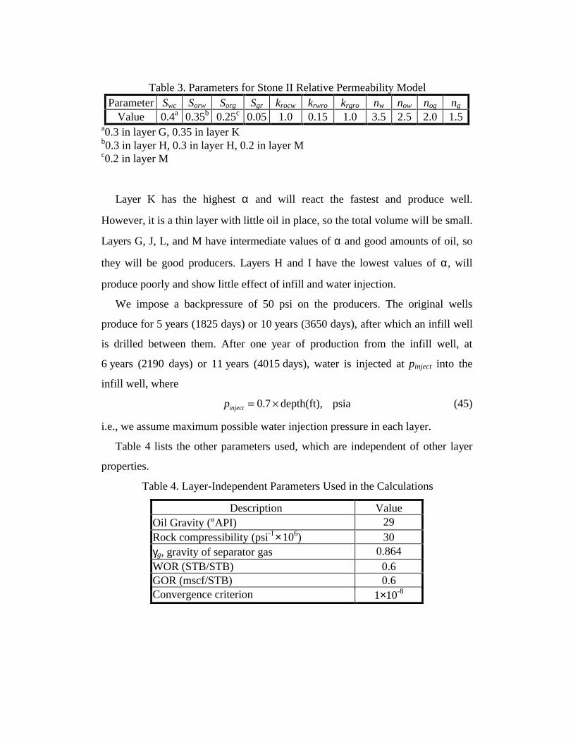
Table 3. Parameters for Stone II Relative Permeability ModelParameter Swc Sorw Sorg Sgr krocw krwro krgro nw now nog ng

Value 0.4a 0.35b 0.25c 0.05 1.0 0.15 1.0 3.5 2.5 2.0 1.5a0.3 in layer G, 0.35 in layer Kb0.3 in layer H, 0.3 in layer H, 0.2 in layer Mc0.2 in layer M

Layer K has the highest α and will react the fastest and produce well.

However, it is a thin layer with little oil in place, so the total volume will be small.

Layers G, J, L, and M have intermediate values of α and good amounts of oil, so

they will be good producers. Layers H and I have the lowest values of α, will

produce poorly and show little effect of infill and water injection.

We impose a backpressure of 50 psi on the producers. The original wells

produce for 5 years (1825 days) or 10 years (3650 days), after which an infill well

is drilled between them. After one year of production from the infill well, at

6 years (2190 days) or 11 years (4015 days), water is injected at pinject into the

infill well, where

pinject = �0 7. depth(ft), psia (45)

i.e., we assume maximum possible water injection pressure in each layer.

Table 4 lists the other parameters used, which are independent of other layer

properties.

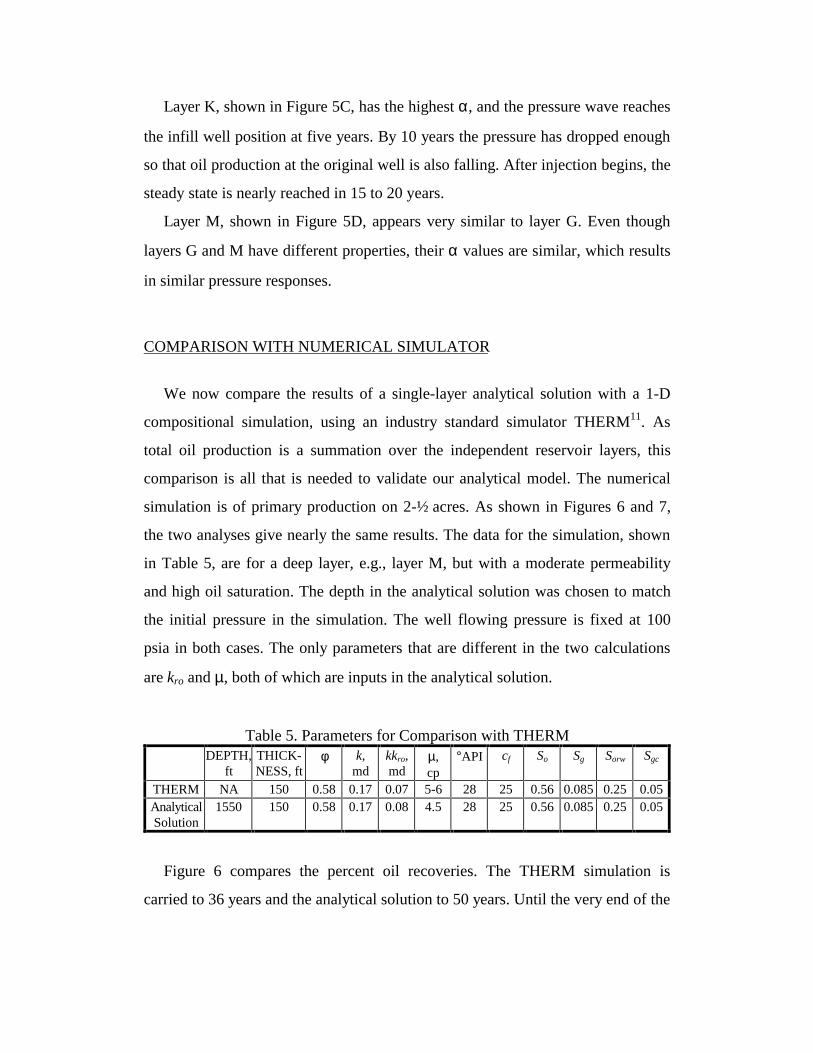
Table 4. Layer-Independent Parameters Used in the Calculations

Description ValueOil Gravity (°API) 29Rock compressibility (psi-1× 106) 30γg, gravity of separator gas 0.864WOR (STB/STB) 0.6GOR (mscf/STB) 0.6Convergence criterion 1×10-8

These parameter values are used to calculate the pressure, oil flow rate at the

wells, and cumulative oil production from each layer as a function of time. The

cumulative production and percent oil recovery are of most interest, and the

results are shown in the following figures as a function of the square root of time,

giving straight lines for early times. All calculations are carried out for 50 years

(18,250 days = 135 day1/2).

Figure 1 shows the cumulative production in thousands of barrels in each layer

and the total for 50 years without infill or injection. The slope of the total primary

production is approximately 3000 STBO/day1/2, which is representative of a very

good well in the diatomite. A poorer well might not have the entire hydrofracture

area open, or it might have and the production would be less.

Layer G, which has the most oil in place and high α, produces the most oil.

The next two layers, H and I, have low oil saturations and low α values and are

poor producers. The deeper layers have high α values and are good producers.

Layer K has a low cumulative production because it has little oil in place.

Figure 2 shows the percent oil recovery of all of the layers and the total for 50

years. The total is recovery is about 10 percent, with the deeper layers J through M

better and the top layers G through I worse.

Figure 3 shows the percent oil recovery and water injection for infill at 5 years

and water injection at 6 years. Figure 4 shows the same results for infill at 10

years and water injection at 11 years. These figures show the percent oil recovery

and water injection for each layer in the formation calculated as the volume

produced or injected divided by the original oil in place times 100. The final total

increase in recovery from injection is about 3 percent. The scale of each figure,

except layer K, is the same so that the layers can be easily compared.

Each of the plots has five separate curves. The top curve, shown as a bold solid

line, is the percent oil recovery from the original well, including the effect of the

infill well and water injection. The upward trend at late times is from the extra oil

produced by water injection. The normal solid line is the percent oil recovery at

the original well with infill but without injection at the infill well. In most of the

layers, the difference between recovery with and without injection is about 3

percent. In layer K the effect is rapid and large, because of the high α. However,

we stress that much of the increased recovery in this layer at late times may be just

from the injected water recirculated through the producer. Layers H and I show

almost no effect of the water injection because of low oil saturation and low α.

This calculation shows that in the absence of Buckley-Leverett banking of oil, the

incremental oil recovery from pressure support by water injection will be small.

Hence, in layers with a low oil saturation or unfavorable mobility ratio, one

cannot expect a big waterflood response.

The first dotted curves show the percent oil recovery at the infill well where

production starts from zero at the infill time. The “Infill (no injection)” curves in

Figures 3 and 4 show the production if there were no injection, and the “Infill

(with injection)” curves show the production with injection. These latter recovery

curves (including water injection) become flat after water injection begins because

no more oil is produced at the infill well. For most of the layers, a significant

amount of oil production from the infill well is lost because of injection.

However, injection may be necessary to preserve the integrity of the formation

and decrease well failure. Thus, producing from the infill well for two to five

years before injection begins instead of just one may be better.

The water injection curve is the volume of water injected divided by the

original oil in place in the layer times 100 to keep the units consistent. Even

though the injection begins at about six years, the effect at the original wells is not

seen until almost 20 years. Layer K shows the effect sooner, but layers H and I

show almost no effect of injection even at 50 years. The rate of water injection

becomes constant at late times. The percent recovery rises linearly with time for

late times, but appears to bend upward when plotted here versus the square root of

time.

To further explain the figures, we specifically consider layer G. We see from

Figure 1 that the total volume of oil produced in 50 years is approximately 100

MSTBO with no infill or injection, which is about 8 percent recovery. With infill

and injection the original well produces just under 9 percent or 110 MSTBO, and

the infill well produced an additional 15 MSTBO in the one year of production.

The 15 MSTBO could be increased to about 30 MSTBO if water injection began

at eight years instead of six.

Figure 5 shows the pressure profiles for infill at 10 years and water injection at

11 years for layers G, I, K, and M. These layers show representative values of α

with layer I having the lowest and layer K the largest value. Large values of α give

a faster pressure response. In these figures, the position labeled 0 feet is the

position of the infill well, and the position at 165 feet is the original well. The

pressure at the original well is constant at 50 psia.

In Figure 5A, the initial pressure in layer G is 350 psia and the pressure at the

“original” well is maintained at 50 psia. The pressure profile at x = 0 is horizontal

until 10 years, indicating the no-flow (or symmetry) boundary condition. At

10 years when the infill well is drilled, the pressure at x = 0 has not decreased

significantly. The 11th year profile is just before injection at 513 psia begins at the

infill well. Finally, the pressure distribution becomes a linear, steady-state profile

with injection.

Layer I, shown in Figure 5B, reacts much slower than the other layers. The

initial pressure is 480 psia. By 10 years when the infill well is drilled, the pressure

wave is only about a quarter of the way in from the original well. Even at 50

years, the steady state is not yet reached. The infill and injection does not

significantly affect the original well.

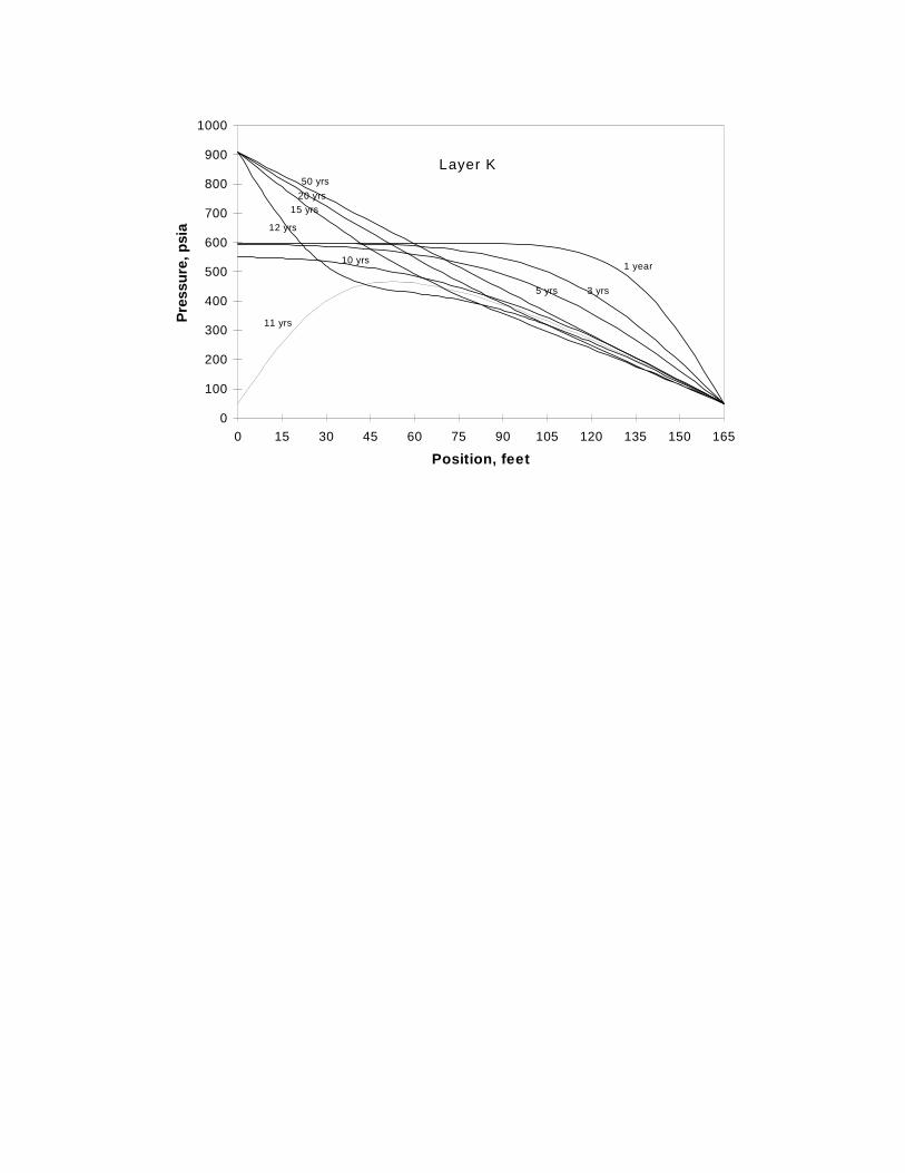
Layer K, shown in Figure 5C, has the highest α, and the pressure wave reaches

the infill well position at five years. By 10 years the pressure has dropped enough

so that oil production at the original well is also falling. After injection begins, the

steady state is nearly reached in 15 to 20 years.

Layer M, shown in Figure 5D, appears very similar to layer G. Even though

layers G and M have different properties, their α values are similar, which results

in similar pressure responses.

COMPARISON WITH NUMERICAL SIMULATOR

We now compare the results of a single-layer analytical solution with a 1-D

compositional simulation, using an industry standard simulator THERM11. As

total oil production is a summation over the independent reservoir layers, this

comparison is all that is needed to validate our analytical model. The numerical

simulation is of primary production on 2-½ acres. As shown in Figures 6 and 7,

the two analyses give nearly the same results. The data for the simulation, shown

in Table 5, are for a deep layer, e.g., layer M, but with a moderate permeability

and high oil saturation. The depth in the analytical solution was chosen to match

the initial pressure in the simulation. The well flowing pressure is fixed at 100

psia in both cases. The only parameters that are different in the two calculations

are kro and µ, both of which are inputs in the analytical solution.

Table 5. Parameters for Comparison with THERMDEPTH,

ftTHICK-NESS, ft

φ k,md

kkro,md

µ,cp

°API cf So Sg Sorw Sgc

THERM NA 150 0.58 0.17 0.07 5-6 28 25 0.56 0.085 0.25 0.05AnalyticalSolution

1550 150 0.58 0.17 0.08 4.5 28 25 0.56 0.085 0.25 0.05

Figure 6 compares the percent oil recoveries. The THERM simulation is

carried to 36 years and the analytical solution to 50 years. Until the very end of the

numerical simulation, the results are similar. The simulation predicts a lower

ultimate recovery, because depletion changes the properties of the system. Thus α

is not actually constant for the entire production time because the volatile oil

components are produced preferentially. However, the difference is not significant

until after 30 years.

Figure 7 compares the average pressure in the layer. The analytical solution

uses Eq. (10). The average pressure predicted by the analytical solution falls

slightly slower than that predicted by THERM. Also near the end of the

simulation, the pressure flattens out more quickly, and the production slows down.

This is caused by the preferential depletion of solution gas in the simulation and

gradual decrease of overall system compressibility.

Our simple analytical model can accurately predict the recovery and pressures

for primary production. The PVT properties and relative permeabilities agree well

with those predicted by THERM.

CONCLUSIONS

We have presented a complete analytical model of transient, linear flow for

single-phase flow in a low-permeability, layered, and compressible reservoir on

primary. Further considerations should include the effects of Buckley-Leverett

displacement, as well as the effects that production and injection may have on the

formation, the fluid properties, and the hydraulic diffusivity. However, the current

analysis gives a good estimate of the fluid production and time-scales of interest

for a heterogeneous, low-permeability, layered reservoir.

1. We have considered primary fluid recovery on the original well spacing,

followed by an infill program and conversion of the infill wells to water

injectors.

2. Our analysis is simplified and has many limiting assumptions. It is not meant

to be a replacement for a reservoir simulation, but, being an analytical

solution, it demonstrates the effects of the system parameters on the solution.

3. A single-layer analytic solution agrees well with a fully compositional

numerical simulation.

4. The calculations presented here are for the South Belridge Diatomite and

should give reasonable estimates of the diatomite layer productivities.

5. We give an estimate of when to drill an infill well and how long to produce

from the infill well before converting it to an injector. Our analysis predicts

that about 9% of OOIP can be recovered on 2-1/2-acre primary in a good

portion of the South Belridge Diatomite. The infill to 1-1/4 acres, followed by

a conversion of the infill well to a water injector, increases the ultimate

recovery by another 3% of OOIP.

6. Hence, in the absence of a strong Buckley-Leverett banking of the oil and/or

strong capillary imbibition, the effect of pressure support by water injection on

the incremental oil recovery is weak. In lower quality reservoirs (layers or

fields), the effect of waterflood may be small.

7. Another important result is the quantification of reservoir heterogeneity. This

analysis helps identify the good layers and those layers with fast pressure

responses.

8. The current analysis gives a good estimate for the pressure, production rate,

and cumulative production from original wells, with infill producers drilled at

some later time and then converted to water injectors. Our model can predict

the onset of pressure depletion and quantify the duration of production from

the infill wells before injecting water.

9. We show that producing from the infill well for a few years significantly

accelerates the production from the field and can minimize the loss of

production at the infill well caused by conversion to a waterflood injector.

ACKNOWLEDGEMENTS

This work was supported by two members of the U.C. Oil® Consortium,Chevron Petroleum Technology Company, and Aera Energy, LLC. Partial supportwas also provided by the Assistant Secretary for Fossil Energy, Office of Gas andPetroleum Technology, under contract No. DE-ACO3-76FS00098 to theLawrence Berkeley National Laboratory of the University of California.

NOMENCLATURE

°API = oil gravity

A = twice the area of the production hydrofracture, ft2

B = volume formation factor, RB/STB or RB/scf

c = compressibility, 1/psi

erfc= complimentary error function

GOR = gas-oil ratio, scf gas/STB oil

k = absolute permeability of the formation, millidarcies

kro = relative permeability for oil

krw = relative permeability for water

krg = relative permeability for gas

krow = relative permeability for two-phase oil/water system

krog = relative permeability for two-phase oil/gas system

krocw = relative permeability to oil at connate water saturation

krwro = relative permeability to water at residual oil saturation

krgro = relative permeability to gas at residual oil saturation

L = half-spacing of original wells, ft

m = summation index

n = summation index

nw = water relative permeability exponent

now = oil/water relative permeability exponent

nog = oil/gas relative permeability exponent

ng = gas relative permeability exponent

P = absolute pressure in the formation, psia

p = pressure in analytical solution, psia

p = average pressure in analytical solution, psia

pbp = bubblepoint pressure, psia

pi = initial formation pressure, psia

pinj = pressure in injection superposition equations, psia

pinject = water injection pressure, psia

pnet = net (total) pressure with infill and injection, psia

pwell = well flowing pressure, psia

Q = cumulative amount, MB

q = flow rate, MBPD

Rs = dissolved gas-oil ratio, scf/STB

Rsw = dissolved gas-water ratio, scf/STB

Swc = connate water saturation

Sorw = residual oil/water saturation

Sorg = residual oil/gas saturation

Sgr = residual gas saturation

T = temperature in the formation, °F

t = time after original production begins, days

tinf = time when infill well begins production, days

tinj = time when water injection begins, days

WOR = water-oil ratio, STB water/STB oil

x = distance from centerline between original wells, ft

Greek Symbols

α = total fluid mobility, ft2/day

βm = eigenvalue

g go = gravity of gas dissolved in oil at a given pressure

g g = gravity of separator gas (sum of free gas and solution gas)

g o = oil gravity

µ = viscosity, cp

λ = mobility, md/cp

λn = eigenvalue

φ = porosity

Subscripts

f = formation

g = gas

inf = infill

inj = injection

o = oil

t = total

w = water

Superscripts

(1) = original well

(2) = infill well

net = total including infill and injection

REFERENCES

1. Schwartz, D. E.: “Characterizing the Lithology, Petrophysical Properties,and Depositional Setting of the Belridge Diatomite, South Belridge Field,Kern County, California,” Studies of the Geology of the San JoaquinBasin, S. A. Graham and H. C. Olson (eds.), The Pacific Section Society

of Economic Paleontologists and Mineralogists, Los Angeles, CA (1988)281-301.

2. Patzek, T. W.: “Surveillance of South Belridge Diatomite,” paper SPE24040 presented at the 1992 Soc. Pet. Eng. Western Regional Meeting,Bakersfield, CA, Mar. 30 - Apr. 1.

3. Nikravesh, M., A. R. Kovscek, and T. W. Patzek: “Prediction ofFormation Damage During Fluid Injection into Fractured Low-Permeability Reservoirs Via Neural Network,” The SPE FormationDamage Symposium, Lafayette, LA, February 14-15, 1995.

4. Nikravesh, M., A. R. Kovscek, A. S. Murer, and T. W. Patzek: “NeuralNetworks for Field-Wise Waterflood Management in Low-Permeability,Fractured Oil Reservoirs,” paper 35721 presented at the 66th Soc. Pet.Eng. Western Regional Meeting, Anchorage, AK, May 22-24, 1996.

5. Kovscek, A. R., R. M. Johnston, and T. W. Patzek: “Interpretation ofHydrofracture Geometry Using Temperature Transients I: ModelFormulation and Verification,” In Situ 9, 221-250 (Sept. 1996).

6. Kovscek, A. R., R. M. Johnston, and T. W. Patzek: “Interpretation ofHydrofracture Geometry Using Temperature Transients II: AsymmetricHydrofractures,” In Situ 9, 251-289 (Sept. 1996).

7. Carslaw, H. S., and J. C. Jeager: Conduction of Heat in Solids, 2nd Ed.,Clarendon Press, Oxford (1959).

8. Ahmed, T.: Hydrocarbon Phase Behavior, Contributions in PetroleumGeology and Engineering 7, Gulf Publishing Company, Houston, TX(1989) 424.

9. Standing, M. B.: A Pressure-Volume-Temperature Correlation forMixtures of California Oils and Gases, API Drilling and ProductionPractice 275 (1947).

10. Beggs, H. D., and J. R. Robinson: “Estimating the Viscosity of Crude OilSystems,” Journal of Petroleum Technology 27 (1975) 1140-1141.

11. THERM, Scientific Software-Intercomp, Inc., 1801 California, Suite 295,Denver, CO 80202-2699.

APPENDIX A: Total Hydraulic Diffusivity and PVT Properties of Oil, Gas andWater

All of the formation and fluid properties are combined into the single

parameter α, the hydraulic diffusivity of the fluid-rock system. We assume that α

is constant and calculated using the initial formation and fluid conditions such as

pressure, temperature, saturation, etc. We define α by

α λφ

= 0 006336. t

tc, ft / day2 (A.1)

where λt is the total fluid mobility in the reservoir, md/cp, φ is the porosity, and ct

is the total volume-weighted compressibility, 1/psi, of the system consisting of

rock, f, oil, o, water, w, and gas, g.

The total fluid mobility is

l l l lt o w g= + + , (A.2)

or

λ λ λ λ λ λt o w o g o= + +1 / / ,c h md / cp . (A.3)

This equation for the total mobility can be expressed through the surface-

measured quantities: the water-oil ratio, WOR in STB water/STB oil, and the gas-

oil ratio, GOR, scf gas/STB oil

l lt ow

o

g

o

B

B

B

B= + +

��

��1 WOR GOR , (A.4)

where Bo is the oil volume formation factor, RB/STB, Bw is the water volume

formation factor, RB/STB, and Bg is the gas volume formation factor, RB/scf.

The oil mobility is defined as

λµo

ro

o

kk= (A.5)

We use the Stone II model given later in this Appendix to calculate the oil

relative permeability.

The total system compressibility is

c c S c S c S ct f o o w w g g= + + + , 1 / psi (A.6)

which can be calculated as

c c SB

B

P

B

B

R

PS

B

B

P

B

B

R

P

S

B

B

Pt f oo

o g

o

sw

w

w g

w

sw g

g

g= + - +��

�� + - +

��

�� -

1 1��

��

��

��

��

(A.7)

We now define the functions used to calculate the PVT properties of the

formation and the fluids. We calculate these properties at the bubblepoint. In what

follows, we use general correlations8-10 of the fluid PVT properties. The

coefficients of these correlations have not been optimized for the diatomite crude-

solution gas system.

Dissolved Gas-Oil Ratio, Rs (scf/STB)9

R Ps g go= +γ γ/ . .4

.18 2 1

1 2048a f (A.8)

where

γ go = °10 0 0125{ . ( API)-0.00091T}

Live Oil Viscosity, µo (cp)10

m mo odBA= (A.9)

where

A Rs= + −12 859 200

0 482.

.b g , B Rs= + −1 276 15

0 090.

.b g

Dead Oil Viscosity, µod (cp)10

modx= -10 1 (A.10)

where

x yT= −0 601. , y z= 10 , z = − °2 1646 0 033580. . APIa f

Oil Formation Volume Factor, Bo (RB/STB)9

B Fo = +0 97759 0 000120 1 20. . .a f (A.11)

where

F R Ts g o= +γ γ/ ..c h0 5

1 25 , g o = +�141 5 131 5. / . API0 5

Gas Formation Volume Factor, Bg (RB/scf)9

B Z T Pg = +0 005035 459 6. . /0 5 (A.12)

where

Z A A e CpBprD= + - +10 5 /

A T Tpr pr= - - -139 0 92 0 36 0 1010 5

. . . ..2 7

B T pT

p ppr pr

pr

pr T prpr

= - +-

-�!

"$## +

-

0 62 0 230 066

0 860 037

0 32

10

2

9 1

6. ..

..

.2 7 2 7 3 8

C Tpr= −0 132 0 32 10. . logc h

DT Tpr pr= - +

100 3106 0 49 0 1824 2. . .3 8

T T Tpr pcM= + �459 6. /0 5p P ppr pcM= �/

� = -T TpcM pcM e

� =-

+ -p

p T

T y ypcm

pcM pcM

pcM

e

e2 7

3 8H S H S2 21

e = + - + + -120 150 9 1 6 0 5 4y y y y y yCO H S CO H S CO H S2 2 2 2 2 2

3 8 3 8 3 8. . .

T y y y T y y ypcM pcHC= - - - + + +1 227 548 672N CO H S N CO H S2 2 2 2 2 23 8

p y y y p y y ypcM pcHC= - - - + + +1 493 1071 1306N CO H S N CO H S2 2 2 2 2 23 8

TpcHC gHC gHC= + -187 330 715 2g g.

ppcHC gHC gHC= - -706 51 7 111 2. .g g

gg

gHCg y y y

y y y=

- - -- - -

0 967 1 52 118

1

. . .N CO H S

N CO H S

2 2 2

2 2 2

yCO2 = mole fraction of CO2 in gas phase

yH S2 = mole fraction of H2S in gas phase

yN2 = mole fraction of N2 in gas phase

Water Formation Volume Factor, Bw (RB/STB)

Bw = 1 (A.13)

Oil Compressibility, (1/psi)

cB

B

P

B

B

R

Poo

o g

o

s= - +1 ��

��

(A.14)

where

∂∂

γ γB

P

R

PFo s

g o=+

LNM

OQP

0 000144

0 83001 2114874

0 5 0 2.

. ./

. .c h

∂∂R

P

R

Ps s=

+LNM

OQP0 83001 2114874. .

Gas Compressibility, (1/psi)

cB

B

Pgg

g= - 1 ��

(A.15)

The derivative was approximated by

��B

P

B

P

B P B Pg g g g£ =+ -D

D[ ] [ ]10

10(A.16)

Water Compressibility, cw (1/psi)8

c P

T P P T

w = −

+ × − + × − × ×− − − −

[3. .

. . . . ]

8546 0 000134

4 77 10 0 01052 3 9267 10 8 8 10 107 5 10 6 c hd i (A.17)

Stone II Model for Relative Permeability, kro

The Stone II model uses the results of two-phase relative permeability

expressions in an equation for the three-phase oil relative permeability. The two-

phase expressions are power functions given as

k kS S

S Srw rwrow wc

orw wc

nw

= −− −

LNM

OQP1

(A.18)

k kS S

S Srow rocww orw

orw wc

now

= − −− −

LNM

OQP

1

1(A.19)

k kS S S

S Srog rocwwc org g

wc org

nog

=− − −

− −LNMM

OQPP

1

1(A.20)

k kS S

S S Srg rgrog gr

wc org gr

ng

=−

− − −LNMM

OQPP1

(A.21)

The final expression for the oil relative permeability is

k kk

kk

k

kk k kro rocw

row

rocwrw

rog

rocwrg rw rg= + + − −

LNM

OQP

( )( ) (A.22)

FIG. 1. Cumulative oil production in each layer.No infill or injection.

FIG. 2. Percent oil recovery in the various layersNo infill or injection.

FIG. 3. Percent oil recovery or water injection versus the square root of time,days1/2. Infill at 5 years and injection at 6 years.

FIG. 4. Percent oil recovery or water injection versus the square root of time,days1/2. Infill at 10 years and injection at 11 years.

FIG. 5A. Pressure in layer G, psia, versus the position from infill well, feet.Infill at 10 years and injection at 11 years.

FIG. 5B. Pressure in layer I, psia, versus the position from infill well, feet.Infill at 10 years and injection at 11 years.

FIG. 5c. Pressure in layer K, psia, versus the position from infill well, feet.Infill at 10 years and injection at 11 years.

FIG. 5D. Pressure in layer M, psia, versus the position from infill well, feet.Infill at 10 years and injection at 11 years.

FIG. 6. Comparison of THERM simulation and analytical solution.Percent oil recovery on primary for 50 years.

FIG. 7. Comparison of THERM simulation and analytical solution.Average layer pressure on primary for 50 years.

0

10

20

30

40

50

60

70

80

90

100

0 20 40 60 80 100 120 140

Square Root of Time (days)

Lay

er C

um

ula

tive

Pro

du

ctio

n,

MS

TB

O

0

50

100

150

200

250

300

350

400

450

500

To

tal Cu

mu

lative Pro

du

ction

, M

ST

BO

G

I

J

H

K

L

M

Total

0

2

4

6

8

10

12

14

16

0 20 40 60 80 100 120 140


Per

cen

t O

il R

eco

very

G

H

I

J

K

LM

Total

0

2

4

6

8

10

12

14

0 20 40 60 80 100 120 140


Per

cen

t O

il R

eco

very

or

Wat

er In

ject

ion Original Total

Infill (no injection)

Infill (with injection)

Water Injection

Original (no injection)

Layer G

0

2

4

6

8

10

12

14

0 20 40 60 80 100 120 140


Per

cen

t O

il R

eco

very

or

Wat

er In

ject

ion Original Total



Water Injection


Layer H

0

2

4

6

8

10

12

14

0 20 40 60 80 100 120 140


Per

cen

t O

il R

eco

very

or

Wat

er In

ject

ion Original Total



Water Injection


Layer I

0

2

4

6

8

10

12

14

0 20 40 60 80 100 120 140


Per

cen

t O

il R

eco

very

or

Wat

er In

ject

ion Original Total



Water Injection


Layer J

0

2

4

6

8

10

12

14

16

18

20

0 20 40 60 80 100 120 140


Per

cen

t O

il R

eco

very

or

Wat

er In

ject

ion Original Total



Water Injection


Layer K

0

2

4

6

8

10

12

14

0 20 40 60 80 100 120 140


Per

cen

t O

il R

eco

very

or

Wat

er In

ject

ion Original Total



Water Injection


Layer L

0

2

4

6

8

10

12

14

0 20 40 60 80 100 120 140


Per

cen

t O

il R

eco

very

or

Wat

er In

ject

ion Original Total



Water Injection


Layer M

0

2

4

6

8

10

12

14

0 20 40 60 80 100 120 140


Per

cen

t O

il R

eco

very

or

Wat

er In

ject

ion Original Total



Water Injection


Total

0

100

200

300

400

500

600

0 15 30 45 60 75 90 105 120 135 150 165

Position, feet

Pre

ssu

re, p

sia

1 year

3 yrs5 yrs

10 yrs

11 yrs

12 yrs

15 yrs20 yrs

50 yrs

Layer G

0

100

200

300

400

500

600

700

800

0 15 30 45 60 75 90 105 120 135 150 165

Position, feet

Pre

ssu

re, p

sia

1 year

3 yrs5 yrs10 yrs

11 yrs

12 yrs15 yrs20 yrs

50 yrs

Layer I

30 yrs

0

100

200

300

400

500

600

700

800

900

1000

0 15 30 45 60 75 90 105 120 135 150 165

Position, feet

Pre

ssu

re, p

sia

1 year

3 yrs5 yrs

10 yrs

11 yrs

12 yrs

15 yrs20 yrs

50 yrs

Layer K

0

200

400

600

800

1000

1200

0 15 30 45 60 75 90 105 120 135 150 165

Position, feet

Pre

ssu

re, p

sia

1 year

3 yrs5 yrs

10 yrs

11 yrs

12 yrs

15 yrs

20 yrs50 yrs

Layer M

0

2

4

6

8

10

12

14

16

0 15 30 45 60 75 90 105 120 135 150


Per

cen

t O

il R

eco

very

1-D THERM Simulat ion

1-D Analyt ic al Solut ion

0

100

200

300

400

500

600

700

800

0 15 30 45 60 75 90 105 120 135 150


Ave

rag

e P

ress

ure

, psi

a

1-D THERM Simulat ion

1-D Analyt ic al Solut ion

LINEAR TRANSIENT FLOW SOLUTION Department …gaia.pge.utexas.edu/papers/infill.pdf · LINEAR...

Documents

Transcript of LINEAR TRANSIENT FLOW SOLUTION Department …gaia.pge.utexas.edu/papers/infill.pdf · LINEAR...