Linear Theory, Dimensional Theory, and the Face-Inversion Effect

Linear Theory, Dimensional Theory, and the Face-Inversion Effect

Geoffrey R. Loftus, Martin A. Oberg, and Allyss M. DillonUniversity of Washington

We contrast 2 theories within whose context problems are conceptualized and data interpreted. Bytraditional linear theory, a dependent variable is the sum of main-effect and interaction terms. Bydimensional theory, independent variables yield values on internal dimensions that in turn determineperformance. We frame our arguments within an investigation of the face-inversion effect—the greaterprocessing disadvantage of inverting faces compared with non-faces. We report data from 3 simulationsand 3 experiments wherein faces or non-faces are studied upright or inverted in a recognition procedure.The simulations demonstrate that (a) critical conclusions depend on which theory is used to interpret dataand (b) dimensional theory is the more flexible and consistent in identifying underlying psychologicalstructures, because dimensional theory subsumes linear theory as a special case. The experimentsdemonstrate that by dimensional theory, there is no face-inversion effect for unfamiliar faces but a clearface-inversion effect for celebrity faces.

Understanding the implications of any experimental outcomerequires a fundamental quantitative theory, within whose contextthe numbers constituting the data may be transformed into con-clusions about the underlying processes that generated the data.This article is about the general consequences for eventual con-clusions of deciding to use one such theory or another and aboutthe specific consequences for understanding a well-known phe-nomenon in the domain of face processing.

The article is divided into five sections. In the first section (“TheFace-Inversion Effect”), we describe an extant psychological prob-lem that serves as a vehicle for illustrating the points that we makeregarding theories. In the second section (“Theories to AnalyzeData”), we describe two quantitative theories: The first, traditionallinear theory, is used almost universally within many disciplines,including psychology, whereas the second, dimensional theory, isconsiderably less known and less used. In the third section (“Sim-ulations”), we describe three simulations, whose purpose is toillustrate some costs and benefits of interpreting data using linearand dimensional theory. In the fourth section (“Experiments”), wedescribe three experiments that, given the foundation we haveestablished, allow us to make some tentative conclusions about theface-inversion effect in particular and about face processing ingeneral. Finally, in the fifth section, our General Discussion, we

compare the two theories that we have been considering: We showformal mathematical relations between them, we comment on theadvantages and disadvantages of using one versus the other as atool for inferring the underlying processes that generated a data set,and we articulate the resulting implied conclusions about faceprocessing.

These five sections are designed in pursuit of three interrelatedgoals. The first goal is to demonstrate (yet again) that traditionallinear theory has severe limitations as a basis for conceptualizingproblems and for analyzing and interpreting data. The second goalis to describe the usefulness of dimensional theory and to provideseveral kinds of tutorial information about how to use it as a basisfor interpreting data. The third goal is to provide an insight and anassociated quantitative theory for understanding the circumstancesunder which a face-inversion effect does or does not emerge.

The Face-Inversion Effect

The face-inversion effect (FIE) refers to a finding first reportedby Yin (1969, 1970) and subsequently by many others (see, e.g.,Bradshaw, Taylor, Patterson, & Nettleton, 1980; Diamond &Carey, 1986; Ellis & Shepherd, 1975; Leehey, Carey, Diamond, &Cahn, 1978; Phelps & Roberts, 1994; Phillips & Rawles, 1979;Valentine & Bruce, 1986) that the processing disadvantage ofinverting a visual stimulus is worse for faces than for other kindsof visual stimuli (e.g., houses). The FIE is one of the primary basesfor the claim that face processing is special, i.e., is qualitativelydifferent from processing other visual stimuli: As noted in a classicreview article, for example, “. . . the evidence from the effect ofinversion . . . provides the most direct indication that face recog-nition may involve a unique process” (Valentine, 1988, p. 472).Although Valentine himself concluded otherwise, the debate is stillfar from settled (see, e.g., Kanwisher, McDermott, & Chun, 1997;Kanwisher, Tong, & Nakayama, 1998; Gauthier, Curran, Curby, &Collins, 2003).

In using the FIE to assess face-processing uniqueness or any-thing else, no one would argue that there is a universal FIE—thatis, that a FIE emerges whenever faces are compared with some

Geoffrey R. Loftus, Martin A. Oberg, and Allyss M. Dillon, Departmentof Psychology, University of Washington.

This research was supported by National Institute of Mental HealthGrant MH41637 to Geoffrey R. Loftus. Special thanks are due to JohnDunn and John Palmer, both of whom provided very extensive commentsand insights during all phases of the work. We also thank Danny Bernstein,Mike Burton, James Cutting, Michael Erickson, Colin MacLeod, andGillian Rhodes for very helpful comments and criticisms on previousdrafts. Finally, we thank Rachael Behrens, Lorena Chavez, Michelle Choi,Jessica Cooke, Kelly Kalalau, and Russell McCann for assistance in datacollection.

Correspondence concerning this article should be addressed to GeoffreyR. Loftus, Department of Psychology, Box 351525, University of Wash-ington, Seattle, WA 98195-1525. E-mail: [email protected]

Psychological Review Copyright 2004 by the American Psychological Association2004, Vol. 111, No. 4, 835–863 0033-295X/04/$12.00 DOI: 10.1037/0033-295X.111.4.835

835

other stimulus type. Rather, the question is almost invariably“under what circumstances does a FIE emerge or not emerge?” Forinstance, a FIE has been claimed to emerge for 10-year-old chil-dren but not 6- or 8-year-old children (Carey & Diamond, 1977),for faces learned normally but not for faces learned as parts (Farah,Tanaka, & Drain, 1995), in a recognition task but not in a matchingtask (Bruyer & Velge, 1981; see discussion by Valentine, 1988, p.474), and for naıve observers but not for experts in the alternativestimulus class (Diamond & Carey, 1986). In short, the quest isusually for the effect of some other variable on the FIE, andseeking such interactions has been a staple of face-processingresearch. It is our hope that in the course of our discussion, we willboth clarify the consequences of using one theory or another tointerpret data (our major goal) and elucidate the issue of when theFIE does or does not emerge (our secondary goal).

Theories to Analyze Data

Below, we report three simulations and three analogous exper-iments concerning the FIE. The simulations and experiments allhave the same general design, which we briefly describe here inorder to provide a context for our discussion of theory. In thesimulations and experiments, Faces or non-Faces (Houses or City-scapes) are shown in a study phase, followed by an old-newrecognition test. At study, stimuli are shown upright or inverted forvarying exposure durations. Thus, there are three independentvariables: exposure duration at study, orientation at study, andstimulus type.

A comment about notation is useful here. We index duration byi, orientation by j, and stimulus type by k. In the simulations andexperiments that we report, there can be an arbitrarily large num-ber, I, of durations; hence, duration is designated di, where i � {1,2, . . . , I}. There are always J � 2 orientation levels, Upright andInverted; hence j � {U, I}. There are always K � 2 stimulus types,Faces and non-Faces. Because non-Faces are mostly Houses, wefind it notationally convenient to let k � {F, H}. We use thisindexing notation extensively throughout this article, it plays acentral role in our discourse, and we urge the reader to mem-orize it.

We now discuss the two theories within whose context we willanalyze and interpret the data from these experiments: lineartheory and dimensional theory. For ease of discourse, we establishhere the subtle but useful distinction between a structure and atheory: A structure is a representation of the information andinformation processing that characterizes some system, whereas atheory is a set of assumptions concerning the structure’s nature thatis used to guide the analysis of that structure. Below, we willdiscuss linear theories designed to describe linear structures anddimensional theories designed to describe dimensional structures.

Linear Theory

The vast majority of experiments in many disciplines, includingpsychology, are designed, analyzed, and interpreted within thecontext of general linear theory. Linear theory, described at leastimplicitly in any statistics text and explicitly in any mathematicallybased statistics text (e.g., Hays, 1973), holds that the dependentvariable in an experiment is the sum of terms corresponding tomain effects of and interactions among independent variables. In

the present experiments with three independent variables, proba-bility, pijk in the condition defined by level i of exposure duration,level j of orientation, and level k of stimulus type, is

pijk � � � �i � �j � �k � �ij � �ik � jk � ijk � error terms,

(1)

where � is the grand mean; �i, �j, and �k are main effects ofexposure duration, orientation, and stimulus type, respectively; �ij,�ik, and jk are two-way interaction effects; ijk is the three-wayinteraction effect; and “error terms” are all the error terms appli-cable given the particular design of the experiment. A FIE withinthe context of this linear theory consists of a linear structure thatincludes a set of nonzero, appropriately signed orientation �stimulus type interaction terms, jk; conversely, lack of a FIEconsists of a linear structure with all jk � 0.

Although linear theory has been a standard tool in understandingmyriad data sets, it has some serious disadvantages (see, e.g.,Loftus, 2002, pp. 343–344). Briefly, they are as follows. First,linear theory is entirely linear, hence its name. Although linearitymay bear an approximation to some actual psychological relations,many other such relations are decidedly nonlinear, which meansthat investigating them within the context of linear theory producesprofoundly misleading results. A classic example of this probleminvolves interpretations of interactions (see, e.g., Bogartz, 1976;Loftus, 1978, 1985; Loftus & Bamber, 1990): As interpretedwithin the context of linear theory, nonordinal interactions ob-served with one dependent variable (e.g., recognition performance)can disappear or reverse with another dependent variable (e.g., d�)or a theoretical construct (e.g., “memory strength”) that is mono-tonically but nonlinearly related to the dependent variable.

The second disadvantage of linear theory is more subtle but alsomore insidious: Because linear theory is both seductively plausibleand almost universally welcomed, it blinds investigators to alter-native theories that might better elucidate underlying psychologi-cal processes. We will argue that dimensional theory includesmany such theories as special cases.

Dimensional Theory

The general idea of dimensional theory is that independentvariables combine at various stages into internal psychologicaldimensions that underlie performance. By determining (a) howmany such dimensions are necessary to account for performance ina given situation along with (b) the nature of the mathematicalfunctions that describe how the independent variables combine toproduce the dimensional values, the underlying nature of therelevant structures can be unveiled.

Dimensional theory is related to conjoint measurement (e.g.,Krantz, Luce, Suppes, & Tversky, 1971; Krantz & Tversky, 1971;Tversky & Russo, 1969), functional measurement (e.g., Anderson,1974, 1979), multidimensional scaling (e.g., Kruskal, 1964; Shep-ard, 1962), the concept of integral and separable dimensions (Gar-ner, 1974), and the concept of “mental modules” (Pinker, 1997).The incarnation of it with which we are concerned here wasindependently described by Bamber (1979) and Dunn and Kirsner(1988), although it was not called “dimensional theory” in eitherarticle. Dimensional theory has proven useful in illuminating var-ious psychological phenomena, including visual displacement dis-

836 LOFTUS, OBERG, AND DILLON

crimination (Palmer, 1986a, 1986b); the relation between iconicmemory and visible persistence (Loftus & Irwin, 1998); the rela-tion between confidence and accuracy in face recognition (Busey,Tunnicliff, Loftus, & Loftus, 2000); the relation between degree oforiginal learning and forgetting rate (Loftus, 1985; Loftus & Bam-ber, 1990); the relations among stimulus duration, stimulus con-trast, confidence, and accuracy in visual recognition (Harley, Dil-lon, & Loftus, 2004); and the logical, theoretical, and empiricalunderpinnings of the dissociation technique (Dunn & Kirsner,1988). Dunn and James (2003) have recently offered a techniquefounded on dimensional theory called signed difference analysisand have illustrated its use in addressing three problems withincognition: First, does the “remember-know” distinction in recog-nition memory reflect qualitatively different cognitive states ordifferent regions on some unidimensional scale? Second, do threemeasures of spatial attention—visual search, texture segregation,and location precuing—reflect the same underlying process?Third, is a “dual-route model” of dyslexia proposed by Coltheart(e.g., Coltheart, 1985) viable?

Dimensional theory is central within vision science. Two exam-ples of its use there are as follows. The first is that of colormetamers: that an indefinitely large number of independent vari-ables, in the form of different monochromatic hues, reduce, in theform of cone quantum-catch values, to three retinal-output dimen-sions whose values determine color perception. The second isBloch’s law: that the two independent variables of stimulus dura-tion and stimulus intensity combine multiplicatively into a singledimension of “total intensity” whose values determine brightnessperception.

D-Dimensional Theory

By dimensional theory, a particular combination of M indepen-dent variables in some experiment yields D values—one on eachof D internal psychological dimensions. Thus,

V2 � f1�IV1, IV2, . . . , IVM�V2 � f2�IV1, IV2, . . . , IVM�

···VD � fD�IV1, IV2, . . . , IVM�,

(2)

where the IV’s are the independent variables, the Vd’s are thevalues on the D dimensions, and the fd’s are unconstrained func-tions. The D values are then mapped to N dependent variables,

DV1 � g1�V1, V2, . . . , VD�DV2 � g2�V1, V2, . . . , VD�

···DVN � gN�V1, V2, . . . , VD�,

(3)

where the DVn’s are the dependent variables. When D � 1, that is,when there is only a single dimension, g1 � g is monotonic. WhenD � 1, the situation is somewhat more complicated, but the gn’sare still constrained in a manner described by Dunn and James(2003). Equations 2 and 3 thereby define a D-dimensional struc-ture. If the inferred number of internal dimensions, D, is less thanthe number of independent variables, M, one concludes that at leasttwo of the independent variables have lost their unique represen-

tations somewhere in the structure, when they merge into fewerdimensions.

We are by no means the first to suggest this kind of structure.The distinction between dimensional values and the relations be-tween these values and the dependent variable has been embodiedin the distinction between a structural model and a measurementmodel (Busemeyer & Jones, 1983) or between an integrationfunction and a response function (Anderson, 1981). Similarly, andmost recently, Dunn and James (2003) used the term structuralmapping in reference to a set of functions relating the V1, . . . , VD

to performance expressed in terms of an abstract, unobservable,psychological metric and the term measurement mapping in ref-erence to a set of monotonic functions relating the psychologicalmetric to observable performance. Dunn and James’s character-izations have the advantage of making a very clear distinctionbetween the central psychological assumptions of the theory (ex-pressed by the structural mapping) and the necessary, although lessinteresting, relation between the performance expressed in terms ofthe psychological metric and performance expressed in terms ofthe actual dependent variable.

An illustration of a dimensional structure is found in colormetamers, mentioned above. Suppose that a mixture of M mono-chromatic hues of differing intensities is presented to the visualsystem. Each hue acts as an independent variable; thus the differ-ent experimental conditions correspond to the different combina-tions of hue intensity. It has long been known that the sensoryresult of any combination of such hue intensities can be describedcompletely by the three numbers corresponding to the three conequantum catches engendered by that combination. Therefore, anydependent variable used to measure color perception in this kind ofexperiment depends only on D � 3 dimensions corresponding tothe output of the three cone classes. This finding, embodied in theclassic color-matching experiment, was pivotal in color science: Itformed the basis for the trichromacy theory of color vision and laidthe groundwork for the eventual discovery of cone photoreceptors.

Unidimensional Theory

The simplest dimensional theory is a unidimensional theory inwhich D � 1; that is, only a single dimension is required toaccount for a data set. An illustration of unidimensional theory isBloch’s law, mentioned above, which describes the results of anexperiment in which different stimulus durations and stimulusintensities are combined. Bloch’s law states that when duration isless than some threshold (around 100 ms), performance—measured, for example, by detection—depends only on the prod-uct of duration and intensity; in other words, the two independentvariables, duration and intensity, combine (multiplicatively) toproduce a value on the D � 1 dimension of “summed intensity.”This means that neither the physical value of duration nor thephysical value of intensity is represented within the sensory sys-tem; rather, only their product is represented. This finding wasuseful in understanding how the sensory system processes inten-sity; viz., for a certain period, about 100 ms, the system simplyintegrates arriving photons over time and maintains a representa-tion of the photon sum.

A unidimensional theory is somewhat akin to a null hypothesiswithin a linear theory: It is a default version of the theory that ingeneral, is tested first. However, a unidimensional theory is unlike

837LINEAR AND DIMENSIONAL THEORIES

most null hypotheses in an important respect. Usually a nullhypothesis is deliberately constructed so as to be uninteresting, andthe investigator’s goal is to reject it. In contrast, a unidimensionaltheory such as Bloch’s law is generally viewed as simple andelegant: If a unidimensional theory is correct, it implies strong andinteresting constraints on how some system works. Therefore, aninvestigator generally wants to confirm a unidimensional theory. Ifone must reject unidimensional theory, then one must add theo-retical dimensions until the data can be accounted for.

Depending on the questions to be addressed and the experimen-tal design, many kinds of unidimensional theories may be con-structed. Here we are concerned with the FIE. Accordingly, auseful unidimensional theory to test would be one in which thereis no FIE. A unidimensional theory designed to accomplish thisgoal is as follows. First, the two perceptual variables, duration, d,and orientation, O, combine to produce a value on a single dimen-sion that we will somewhat arbitrarily term S � “Strength”; thus,

S � f�d, O�, (4)

where the function f, although in principle unconstrained, would beexpected to yield higher S values with longer durations, and forupright compared to inverted stimuli. A fundamental element ofsuch a theory has been suggested by Valentine (1988), who notedthat “. . . the available evidence suggests that inversion and briefpresentation affect perception in similar ways” (p. 483). Thecritical element that Valentine does not suggest is that these“similar ways”—formally embodied here in Equation 4, whichstates that duration and orientation both operate in the commoncurrency of Strength—are identical for Faces and non-Faces.

The next component in our unidimensional theory is the map-ping from Strength to recognition performance, which is assumedto be monotonic. However, it makes little sense to assume thatFace performance and non-Face performance are related toStrength in identical ways. There are many reasons to believe thatthe Strength-performance function might differ for the two stim-ulus types; for instance, the set of Faces may be more homoge-neous than the set of non-Faces (or vice versa), or Faces may bemore intrinsically recognizable than non-Faces (or vice versa), andso on. Thus we allow separate monotonic functions relating rec-ognition performance to Strength, namely,

p � �mF�S� for FacesmH�S� for non-Faces , (5)

where p is recognition performance and mF and mH are monotonicfunctions.

We emphasize that within the context of this unidimensionaltheory, the mechanism affected by orientation is embodied only inthe function, f, in Equation 4 that maps a duration � orientationcombination to Strength. At that point, stimulus type has not yetcome into play; rather the stimulus-type effect is embodied in thefunctions, mF and mH, of Equation 5, which operate only onStrength. Therefore, by this unidimensional theory, there is no FIE;that is, there is no direct connection between orientation on the onehand and stimulus type on the other. Below, we describe a formaland unambiguous prediction of this unidimensional theory.

Simulations

The simulations and experiments that we report are designed tosimulate or to investigate the FIE with respect to memorization of

faces in anticipation of an old-new recognition test. As we havenoted, we treat both simulations and experiments primarily as avehicle for discussing theory. However, they are also designed toilluminate a specific aspect of face processing and of the effects offace inversion. In particular, Valentine (1988) has asserted that“the orientation of the inspection series [in a recognition proce-dure] does not appear to be critical [in producing a FIE],” and wenton to conjecture, “Therefore it is possible that the disproportionateeffect of face inversion only emerges when the task involvesrecognizing a face as one stored in memory” (p. 474). If true, thiswould suggest that face inversion does not differentially affectencoding of faces for subsequent recognition but rather affectsprocessing only of already stored faces. Thus our experiments aredesigned to address this issue—to determine whether there is a FIEin a very powerful and stringently controlled experiment in whichorientation is varied only in the study phase of a recognitionprocedure.

Our simulated data were designed to be qualitatively similar tothe data that emerged from our experiments. In each simulation,the data issued from a particular structure, and the data wereanalyzed within the contexts of both linear theory and dimensionaltheory. In Simulation 1, we generate data from a unidimensionalstructure, in which the single dimension is “Strength.” In Simula-tions 2 and 3, we generate data from a linear structure. The linearstructure generating the Simulation-2 data includes a FIE, whereasthe linear structure generating the Simulation-3 data does notinclude a FIE.

To foreshadow our findings, the simulations serve as demon-strations that data interpretation using linear theory produces asomewhat chaotic pattern of results, whereas interpretation usingdimensional theory produces a consistent pattern of results. Weargue that this superiority of dimensional theory over linear theoryis general rather than specific to our demonstrations, and wedescribe underlying reasons why this is so.

Simulation 1: Unidimensional Structure

The method used in all simulations is as follows. Two stimulussets, Faces and Houses, are presumed to have been assembled.Target stimuli are shown, one by one, in the study phase of arecognition experiment. Half the target stimuli are shown upright,while the remainder are shown inverted. A test phase follows inwhich the target stimuli are randomly intermingled with distract-ers, also consisting of Faces and Houses, drawn from the samepopulation as the targets. All test pictures are shown upright, andold-new recognition performance is measured. There are 14 levelsof study exposure duration, ranging from 30 to 420 ms in 30-msincrements. So here, as in all our simulations and experiments,there are three independent variables: stimulus duration (here, 14levels) � orientation (Upright/Inverted) � stimulus type (hereFaces/Houses).

In Simulation 1, we generated data from a unidimensionalstructure defined by Equations 4 and 5. We did so by implement-ing specific versions of the functions f, mF, and mH, selected toproduce data that are qualitatively similar to the data that emergedin the experiments. In particular, to generate Strength, Sij forduration di and orientation j,

Sij � �MU � di for Upright stimuliM1 � di for Inverted stimuli . (6)


To generate recognition performance, pijk,

pijk � � �G�Sij/BF� � 0.5� � YF for Faces�G�Sij/BH� � 0.5� � YH for Houses , (7)

where G(Z) is the cumulative Gaussian probability of a normaldeviate, Z. The free parameters in Equations 6 and 7 are interpretedas follows. MU and MI (Mj � 0) are proportionality constantsmapping exposure duration to Strength for Upright and Invertedstimuli. The four parameters, BF, BH, YF, and YH, specify themonotonic functions mapping Strength to probability: The Bk’s (Bk

� 0) are scaling parameters for the Gaussian transformations, andthe Yk’s (0 Yk 2) are asymptotic values (actually asymptoticvalues multiplied by 2, as the bracketed portions of Equation 7produce values between 0.0 and 0.5). These parameter values aredesigned to produce p values in the 0–1 range, which may beinterpreted as probabilities. The six parameter values were set toMU � 1.50, MI � 0.75, BF � 400, BH � 250, YF � 2.0, and YH �1.3.

We emphasize, as we did earlier with respect to the general case,there is no FIE within the context of this unidimensional structure.

Orientation combines with duration to produce a Strength value.Once Strength has been generated, orientation no longer has aunique representation. Face and House performance then dependonly on Strength.

For simplicity, we assume that there is no statistical error, andthat the experiment is perfectly counterbalanced. These assump-tions allow us to directly compare linear theory and dimensionaltheory in their ideal forms when population parameters are knownrather than estimated. We do not, of course, deny the existence ofstatistical error in the real world; however, in the context of thepresent discussions, such error constitutes an add-on complicationwhose consideration serves no useful purpose.

Results

The structure defined by Equations 6 and 7 yields the datashown in Figure 1. Figures 1A and 1B show the main results forFaces and Houses: memory performance as functions of stimulusduration (ignore for the moment the arrows and associated text).Within each panel, there are two curves: In this, as in subsequent

Figure 1. Simulation 1: Hypothetical data generated by a unidimensional structure. All data points are asfunctions of study exposure duration. A and B: Recognition performance for Faces and Houses, respectively; thetwo curves in each panel are for Upright and Inverted stimuli. C: Inversion magnitudes (Upright minus Invertedperformance) for Faces and Houses. D: Face-inversion effect (FIE) magnitude (Face minus House inversionmagnitudes). Subscripts in ordinate labels refer to duration (i), Orientation (j �{U, I}), and Stimulus Type (k �{F, H}).


figures, solid upright triangles represent Upright conditions, andopen inverted triangles represent Inverted conditions. Figure 1Cshows what we refer to as the inversion magnitudes—Uprightperformance minus Inverted performance—for both Faces andHouses, also as functions of duration. Finally, Figure 1D shows theFIE directly, in the form of the difference between the Face andHouse inversion magnitudes.

Although we of course know how these data were generated, wewill for the moment act as if, just like normal investigators, we donot know, would like to find out, and will try to do so using anappropriate analysis and interpretation technique.

Analysis and interpretation within the context of linear theory.We first analyze and interpret the data within the context oftraditional, i.e., linear theory. The equation for linear theory in thisexperiment is Equation 1 above (minus the error terms, as we areassuming no error), where the �i’s, �i’s, and �k’s represent theeffects of duration, orientation, and stimulus type.

A FIE would be implied by an appropriately signed orienta-tion � stimulus type interaction. This interaction—the differencebetween Face and House inversion magnitudes—is shown as afunction of exposure duration in Figure 1D. Its value, averagedacross durations, is 0.077. Overall, therefore, a FIE would beinferred from the results of this experiment.

However, Figure 1D also indicates that the story is more com-plicated: There is an orientation � stimulus type � exposureduration interaction; that is, FIE magnitude varies with exposureduration. In particular, the FIE is virtually nil for stimuli shown foran exposure duration of less than about 100 ms and then increaseswith increasing exposure duration. One might therefore concludethat stimuli must be shown for some threshold duration in orderthat the FIE has a chance to develop.

Analysis and interpretation within the context of dimensionaltheory. In Simulation 1, we are, as noted, in the felicitous posi-tion of knowing the unidimensional structure that produced thedata because we created it. Normally of course, the epistemolog-ical situation is reversed: We collect the data and then analyzethem in quest of inferring the structure that generated them. Howwould we have confirmed that a unidimensional structure under-lies the Simulation-1 data if we didn’t know so to begin with?

The answer is that even a weak unidimensional theory of thesort expressed in Equations 4 and 5 makes a strong and unambig-uous prediction that can be tested via a technique described byBamber (1979) and Dunn and Kirsner (1988). Following Bamber’sterminology, we refer to the technique as state-trace analysis, atutorial on which is provided by Harley et al. (2004; see Harley etal.’s Appendix).

To understand the prediction and the analysis, consider Figure1A. Two conditions—the 210-ms Upright condition and the420-ms Inverted condition—happen to yield identical perfor-mance for Faces ( pF � 0.569). This is indicated by the horizontalarrow connecting the two data points. By Equation 5, this meansthat these two conditions must have produced the same Strengthvalue, specifically S � mF1 (0.569), where the superscript “1”signifies “inverse.” Equation 5 then also implies that because thesetwo conditions have the same Strength value, they must produceequal performance values for Houses, specifically pH � mH(S) �mH[mF

1 (0.569)]. This prediction is confirmed, as indicated bythe horizontal arrow in Figure 1B connecting the correspondingdata points: House performance for both conditions is pH � 0.515.

To maximize this example’s comprehensibility, we deliberatelychose a set of durations and theory parameters that would produceconvenient instances of shorter-duration Upright conditions (e.g.,210-ms Upright) and longer-duration Inverted conditions (420-msInverted) yielding equal performance. However, the success ofstate-trace analysis does not require that one be lucky enough (inreal life) to find such pairs. Instead, unidimensional theory isgenerally tested by constructing a state-trace plot which like thefamiliar receiver-operating characteristic (ROC) of signal-detection theory, is a scatterplot, over experimental conditions, ofone dependent variable (here, House performance) against anotherdependent variable (here, Face performance). The prediction isthat across all conditions—all 28 duration � orientation conditionsin this instance—the scatterplot points must form a monotonicfunction. The reason for this monotonicity prediction is as follows.Consider two duration � orientation conditions, C11 � (d1, O1)and C22 � (d2, O2). Condition C11 gives rise to Strength S11 andto performance values p11F and p11H, whereas Condition C22 givesrise to Strength S22 and to performance values p22F and p22H.Suppose that for Faces, Condition C11 produces poorer perfor-mance than Condition C22, that is, p11F p22F. Because the mk’sare monotonic, they can be inverted to recover Strength, which hasthe same ordering: S11 � mF

1( p11F) mF1 ( p22F) � S22. This, in

turn, means that the ordering of house performance must also bethe same because p11H � mH (S11) mH(S22) � p22H. In otherwords, if this unidimensional theory is correct, then any twoscatterplot points ordered in one way for faces must be ordered inthe same way for houses. This defines a monotonic relation be-tween the two.1

A more complete and formal treatment of this issue is providedby Bamber (1979). Briefly, one assumes that the measured datapoints are samples from an underlying continuous function whoseform can be estimated from the data. Because the continuousfunction is not measured completely but only sampled—the sam-ple corresponding here to the chosen set of stimulus durations—wemust estimate the underlying function by “connecting the dots” inthe scatterplot. Unidimensional theory’s prediction remains thatthe sampled scatterplot points be monotonic. We will see instancesof such monotonic state-trace plots in Simulations 1 and 3 and inExperiment 1. If the scatterplot points are nonmonotonic, we rejectunidimensional theory and are required to posit additional dimen-sions. We will see instances of this process in Simulation 2 and inExperiments 2 and 3.

The state-trace plot for the Simulation-1 data is shown in Fig-ure 2. Again, the solid and open curve symbols represent Uprightand Inverted conditions. On a state-trace plot, two contrast �duration conditions that happen to be equal for both Face andHouse performance appear as two scatterplot points that fall atopone another. The two such conditions that we discussed earlier,and that are indicated in Figures 1A and 1B, indeed appear as twooverlapping points enclosed by the small square in Figure 2.Overall, the scatterplot points form a monotonic function, just as

1 We have one caveat: The foregoing assumes that the functions mk aremonotonically increasing. If instead they were monotonically decreasing,the ordering would change in the inverse transition from pijF to S and thenwould change back in the transition from S to pijH; thus, the end resultwould be the same.


they must, given the underlying unidimensional structure thatgenerated them.

The simplest way of representing degree of monotonicity is witha Spearman rank-order correlation, termed rs. If rs � 1.0, then thefunction is monotonic; if rs 1.0, then the function is nonmono-tonic. The Simulation-1 state-trace plot monotonicity is indicatedat the top of Figure 2 by “rs � 1.000.”

Discussion

We began by creating a simple, unidimensional theoreticalstructure within whose context there was no FIE: Duration andorientation combined to produce a single value of Strength, andonce the duration-orientation combination took place, neither du-ration nor orientation was represented separately. Recognitionperformance was then determined only by Strength, with differentfunctions mapping Strength to recognition performance for the twostimulus types, Faces and Houses. Thus, the performance differ-ence between Faces and Houses is not connected to orientation;rather it occurs only because of differences in the monotonicfunctions, mF and mH, mapping Strength to performance.

Analysis using linear theory. Despite the FIE-less underlyingstructure, analyzing and interpreting the data within the context oftraditional linear theory resulted in the inference of a FIE, based on

the orientation � stimulus type interaction. Moreover, this FIEwas inferred to be somewhat complicated in that its magnitudedepends on the study exposure duration of the stimuli: There isinferred to be no FIE for durations less than about 100 ms, whereasfor durations greater than 100 ms, the magnitude of the FIE isinferred to increase with exposure duration. If such data wereobserved and thusly analyzed in real life, they would doubtlessspark a spirited General Discussion that would include confirma-tion of the FIE’s existence in this paradigm, along with specula-tions about the intriguing manner in which the FIE appears todevelop following the first 100 ms of stimulus processing. Unbe-knownst to the investigator, alas, these conclusions and specula-tions would be entirely without foundation. (We justify thisgloomy assessment below.)

Analysis using dimensional theory. In contrast, analyzing thedata within the context of dimensional theory—that is, construct-ing a state-trace plot and making conclusions accordingly—imme-diately reveals the underlying unidimensional structure that pro-duced the data. One would conclude, given this analysis andinferred structure, that there is no FIE; that is, that in this exper-iment, Faces and Houses are not differentially affected by orien-tation. This conclusion is, of course, contrary to that issuing fromstandard analysis within the context of linear theory, wherein a FIEwas inferred from the orientation � stimulus type interaction.Equally important is that the elegance and simplicity of the theo-retical structure actually responsible for the data is entirely lostwith the classical linear-theory analysis: As we have seen, withinthe context of linear theory, a rather complex and untidy theoret-ical picture emerges.

The generality issue. Above we used the phrase, “withoutfoundation” referring to conclusions about the Figure-1 data basedon linear theory. Is the situation really this grim?

One might argue that because an investigator in real life doesnot know the nature of the structure under investigation, classicallinear theory provides a safe and comfortable haven within whosecontext data should be analyzed and interpreted. That is, in orderto foster communication among investigators and uniformityacross conclusions, it makes sense to agree on a basic theory(linear theory) and then stick to it. On the one hand, we might allagree that linear theory is not quite appropriate to describe manycognitive structures, but on the other hand, we might also agreethat perhaps it provides reasonable approximations to such struc-tures. Given that a particular effect like the FIE can be inferred toexist only within the context of some theory, we may as well inferthe state of its existence using the theory that most of us grew upwith.

A crucial presupposition of such an argument is that there issome degree of generalizability: That is, small variations on thebasic structure that underlies the data—variations that would comeabout from different materials, observers, retention intervals, set-tings, and so on—must, if this argument is to be tenable, produceresults that are at least qualitatively similar to one another. To testthis assumption, we carried out the following exercise. Note firstthat Equations 6 and 7, which generated the Simulation-1 datainclude six free parameters. On each of a series of iterations, werandomly selected new values of these parameters, drawing eachnew parameter from a normal distribution whose mean was theoriginal assigned value (indicated in the paragraph just belowEquation 7) and whose standard deviation was 20% of that mean

Figure 2. Simulation 1: State-trace plot for the Figure-1 hypotheticaldata. House performance is plotted as a function of Face performance.Each data point represents a particular duration for an Upright stimulus(solid upright triangles) or an Inverted stimulus (open inverted triangles).The two overlapping boxed points represent the 210-ms Upright and420-ms Inverted conditions indicated in Figures 1A and 1B by the arrowsand associated text: These two conditions produce equal performance forboth Faces ( pF � 0.569) and for Houses ( pH � 0.515). The rs of 1.000,which refers to the rank-order correlation between all House conditions andall Face conditions, signifies that the state-trace plot is perfectly mono-tonic, thereby correctly confirming a unidimensional theory.


value. We constrained each parameter set so as to produce prob-abilities only in the allowable 0–1 range. We then generated datafrom this new parameter set and examined the FIE. We ran100,000 iterations of this procedure. Each of these 100,000 itera-tions can be viewed as a replication of the original experiment thatproduced the Figure-1 data.

There are several noteworthy results of this enterprise, which areshown in the “Simulation 1” column of Table 1 in the “Linear-theory generalizations for the FIE” section and in Figure 3. Tobegin with, we calculated the mean FIE—the difference of Faceand House inversion magnitudes averaged over durations—foreach iteration. Recall that this value was 0.077 for the Figure-1data. Over all 100,000 iterations, this mean FIE averaged 0.040with a standard deviation of 0.052. Approximately 20% of themean FIE values were negative, while the remaining 80% werepositive.

Figure 3 shows six instances, generated by this process, of FIEmagnitude as a function of duration. They are analogous to theFigure-1D curve, and for comparison, one of them is the originalFigure-1D curve, with the original solid square curve symbols. Allsix of these patterns—the original and the remaining five—arerepresentative of some of the different general patterns thatemerged across the 100,000 iterations. The five new patterns werenot particularly unusual; all turned up within the first 30 iterationsof our 100,000-iteration simulation. Our main point here is thatthese patterns are (loosely speaking) all over the map. Sometimesthe FIE is uniformly negative over all durations, whereas other times it is uniformly positive. Sometimes it monotonically in-

creases or decreases over exposure duration, whereas other timesit is nonmonotonic. All in all, there is not one qualitative aspect ofthe FIE or of the interaction between FIE and duration that remainsconstant across relatively small variations in parameter values.

In contrast to this mess, the monotonic state-trace plot impliedby the unidimensional structure that generated the data to beginwith is guaranteed to show up in every iteration. This fact isunderscored in the “Simulation 1” column of Table 1 in the “Statetrace: Distributions of rs” section where 100% of the 100,000 rs

scores are equal to 1.0.In short, analysis using linear theory to analyze any particular

iteration, that is, any particular experiment in this simulation,would produce one sample from a profoundly chaotic underlyingreality, whereas analysis using dimensional theory would consis-tently reveal the underlying unidimensional structure.

Simulation 2: Positive-FIE Linear Structure

In Simulation 1, we generated data with a unidimensional struc-ture and found that the data were more accurately and consistentlydescribed by dimensional theory than by linear theory. Obviously,it is not especially surprising that the theory corresponding to thestructure which generated the data is better at describing them thana theory corresponding to the structure which did not generate thedata. In Simulations 2 and 3, we generated data from a linearstructure.

In Simulation 2, we wanted to define a simple linear structure inwhich there were the expected main effects of orientation (betterperformance for Upright than for Inverted stimuli) and of duration(better performance for longer durations) along with a positive FIE(greater inversion magnitude for Faces than for Houses), butwithout any other interactions and without a stimulus-type effect.

Table 1Various Measures of Generality for Simulations 1–3

Measure Simulation 1a Simulation 2b Simulation 3c

Linear-theory generalizations for the FIE

M 0.040 0.085 0.023SD 0.052 0.046 0.037Maximum 0.335 0.320 0.172Minimum 0.287 0.113 0.231% 0 19.9 3.1 74.6% � 0 80.1 96.9 25.4

State trace: Distribution of rs (%)

rs 0.95 0.0 33.4 0.00.95 rs 0.96 0.0 18.7 0.00.96 rs 0.97 0.0 0.0 0.00.97 rs 0.98 0.0 44.1 0.00.98 rs 0.99 0.0 0.0 0.00.99 rs 1.00 0.0 3.7 0.0

% rs

1.00 0.0 100.0 0.01.00 100.0 0.0 100.0

% FIE implied

Positive 100.0Negative 0.0

Note. All data are based on 100,000-iteration simulations. FIE � face-inversion effect.a This simulation used a unidimensional structure (no FIE). b This sim-ulation used a linear structure with a positive FIE. c This simulation useda linear structure with no FIE.

Figure 3. Simulation 1: Face-inversion effect (FIE) magnitudes as func-tions of study exposure duration generated by unidimensional structures.The curve with the solid square symbols is the same as the one in Figure1D. The remaining curves result from small variations in the theoryparameters that generated the Figure-1 data.


Achieving this goal proved to be a challenge because the pre-sumed dependent variable in our experiment—recognition proba-bility—is, like many dependent variables, bounded—in this casebetween 1.0 and 0.0—whereas a linear structure, such as the onedefined by Equation 1, is unbounded. In subsequent discussionsections, we have more to say about this issue. For the moment, wesolved the problem by creating the linear structure in terms of avariable that we again call Strength and we again map Strength toprobability using a cumulative Gaussian transform.

In particular, for the ith duration level, jth orientation level, andkth stimulus-type level we define

Sijk � � � di � �j � jk, (8)

where j � {U, I} and k � {F, H}. In keeping with commonlinear-theory notation, we define �j, the one-degree-of-freedomorientation main effect, to be �U, and �I � �U. Similarly, wedefine jk, the one-degree-of-freedom orientation � stimulus typeinteraction terms, to be as shown in Table 2. A positive FIEimplies that UF � 0, whereas no FIE implies that UF � 0 andtherefore that all jk’s be zero.

To map Strength to performance, we again use a Gaussiantransform,

pijk � � �G�Sijk/B�� YF for Faces�G�Sijk/B�� YH for Houses , (9)

where G(Z) is the cumulative Gaussian probability of a normaldeviate, Z. The six free parameter values were set to � � 250,�U � 50, UF � 19, B � 150, YF � 0.7, and YH � 0.9. As inSimulation 1, we assume infinite statistical power and perfectcounterbalancing.

Results

The structure defined by Equations 8 and 9 yields the datashown in Figure 4, which is organized like Figure 1.

Analysis and interpretation within the context of linear theory.As with Simulation 1, we first analyze and interpret the data withinthe context of linear theory. The conclusions are much the same asthey were in Simulation 1: There are main effects of duration andorientation along with a positive FIE whose magnitude averagedover duration is 0.078. Superficially at least, these effects are to beexpected given that they were built into the structure that producedthem, via Equation 8. What is superficially less expected becausethey were not explicitly built into the structure are a duration �orientation interaction (as shown in Figure 4C, the differencebetween Upright and Inverted curves changes over exposure du-ration for both Faces and Houses) and a duration � orientation �

stimulus type interaction, as shown by the inverted U-shaped FIEcurve in Figure 4D.

Analysis and interpretation within the context of dimensionaltheory. Neither a casual look at the Figure-4 data nor a casuallook at Equations 8 and 9 that generated them provides muchinsight about whether the data do or do not conform to a unidi-mensional theory. Intuitively, one would expect that a unidimen-sional theory is sufficiently constrained that it would rarely if evercharacterize data that didn’t actually issue from an underlyingunidimensional structure. Such intuition is confirmed by the state-trace plot, which is shown in Figure 5. Clearly it is nonmonotonic(rs � 0.977), which indicates that the Simulation-2 data do notissue from a unidimensional structure. The particular pattern in thestate-trace plot is instructive: Note that the Inverted data points aredisplaced to the left of the Upright data points. This means that iftwo duration-orientation conditions of the sort indicated in Figure5—a long-duration Inverted condition and a short-duration Up-right condition—are found for which House performance is iden-tical, then for the same two conditions, Face performance is poorerfor the Inverted condition compared with the Upright condition.We have more to say about this kind of data pattern in conjunctionwith its appearance in Experiments 2 and 3; for now, we note thatthis is the kind of state-trace plot pattern that within the context ofdimensional theory implies a positive FIE—a greater deleteriouseffect of inversion on Faces than on Houses.

Generality. We have reported two main findings for Simula-tion 2. First, within the context of linear theory, there was anorientation � stimulus type interaction, of the sort that implied apositive FIE. Within the context of dimensional theory, there wasa systematically nonmonotonic state-trace plot, also of the sort thatimplied a positive FIE. As with Simulation 1, we investigated thegenerality of these findings using the procedure described inconjunction with Simulation 1. We generated data sets usingvariations of the parameter set used in Equations 8 and 9. Eachparameter in a parameter set was drawn from a normal distributionagain with a standard deviation equal to 20% of the mean param-eter value. In addition to constraining the parameter sets to produceonly valid probabilities, we also constrained them to allow onlypositive FIE’s; that is, we excluded any instances of kUF 0. Weagain ran 100,000 iterations.

The results are shown in the “Simulation 2” column of Table 1and in Figure 6. Table 1 indicates that within the context of lineartheory, 96.9% of the iterations produced a positive FIE, whereas,despite the constraint that UF � 0, the remaining 3.1% produceda negative FIE. Figure 6, like Figure 3, indicates that even whenthe underlying structure is explicitly set up to be linear and simple,the observed FIE as well as the relation between FIE and exposureduration is chaotic over small variations of the underlyingstructure.

Within the context of dimensional theory, 100% of the state-trace plots were nonmonotonic, that is, had a less-than-1.0 rs,thereby disconfirming a unidimensional theory. However, thereare two interrelated issues to be contended with. First, disconfir-mation of a unidimensional theory implies only that there is somekind of FIE, without specifying whether it is positive or negative.Second, rejection of unidimensional theory is based on a strictcriterion that one rejects unidimensional theory whenever rs is lessthan 1.0. One might argue that this criterion is too strict, and in reallife, one might fail to reject the null hypothesis of a FIE when rs

Table 2Organization of the Orientation � Stimulus Type InteractionTerms (jk)

Orientation Faces Houses

Upright UF UH � UF

Inverted IF � UF IH � UF

Note. There is only one free parameter, UF.


is close to 1.0, while not requiring rs to be 1.0. We address theseissues in three ways.

First, and most straightforwardly, this argument does not applyto our simulations, which assume no statistical error: For eachiteration, the rs value (and every other statistic) can be accepted as100% accurate. This means that there is no need to equivocateabout the value of rs—either it is 1.0 or it is not.

Second, even in real life, where there is statistical error, theSpearman rs, because it uses ranked data, is a discrete or “grainy”measure; thus, it can yield a value of 1.0 even when the data aresomewhat noisy (unlike, for example, a Pearson r). The graininessin rs is exacerbated to the degree that there are few data points.Even with the 28 data points in our present scatterplots, thegraininess is evident in the “Simulation 2” column of Table 1,where there are no rs values between 0.96 and 0.97 or between0.98 and 0.99. Thus it is reasonable to use a strict criterion of rs 0 to disconfirm a unidimensional theory.

Our third set of comments directly addresses both the issues thatwe have raised. We note that although rs is the most straightfor-ward measure expressing the degree to which a unidimensional

structure may be inferred from a state-trace plot, it is not the onlymeasure. Simply eyeballing the data can provide a start at detect-ing instances when even very high values of rs—even, in fact, anrs value of 1.0—although necessary are not sufficient to reject asingle-dimension theory. This is illustrated in Figure 7, whichshows scatterplots corresponding to various rs values. In everycase, even when rs � 1.0, there is notable divergence between theUpright and Inverted curves.

More important, it is often possible to find empirical functionsthat characterize each of the implied functions within the scatter-plot—in the case of the Figure-5 state-trace plot, for instance, thefunctions relating Houses to Faces for Upright stimuli (solid-triangle data points) and for Inverted stimuli (open-triangle datapoints). Such functions can then be used to infer more precisely thenature of the underlying structure that produced the data. Againharkening to a familiar example, the usual observed cumulativeGaussian form of an ROC curve provides a tool that allows aninvestigator to infer the ratio of signal to noise distribution vari-ances. We will see an instance of this technique in a later sectionwhen we describe specific (linear) functions fitting the real state-

Figure 4. Simulation 2: Hypothetical data generated by a linear structure that includes a positive face-inversioneffect (FIE). A and B: Recognition performance for Faces and Houses, respectively; the two curves in each panelare for Upright and Inverted stimuli. C: Inversion magnitudes (Upright minus Inverted performance) for Facesand Houses. D: FIE magnitude (Face minus House inversion magnitudes). Subscripts in ordinate labels refer toduration (i), orientation (j �{U, I}), and stimulus type (k � {F, H}).


trace plots obtained in Experiments 1–3, along with theoreticalconstraints that are implied by these observed linear functions.

Such functions can be used to determine whether a rejectedsingle-dimension theory implies a positive or a negative FIE. In thepresent instance, we made such a determination as follows. First,we observed that the individual curves in all our simulated state-trace plots could be fit very well by quadratic functions, as shownby the solid lines in Figure 5. Thus, we were able to compute suchquadratic curves for each iteration and to determine the meanamount by which the Inverted curve was displaced to the left of theUpright curve. As we have already described, such a patternimplies a positive FIE. This mean displacement amount was pos-itive, thereby implying a positive FIE, for 100% of the 100,000iterations.

Discussion

The Simulation-2 data were generated by a linear structure inwhich there was a positive FIE. This positive FIE was correctlyinferred from approximately 97% of variants on the data by usinglinear theory and from 100% of variants on the data by usingdimensional theory. Even though these data sets were generated bya linear structure, dimensional theory is perfect in producing thecorrect inference of a positive FIE, whereas linear theory is im-perfect. As was the case in Simulation 1, the relation between theFIE and exposure duration was chaotic over minor changes in thedata structure.

It is apparent that even when the data are generated from a linearstructure to begin with, data interpretation within the context ofdimensional theory produces more coherent and consistent resultsthan interpretation within the context of linear theory. A majorreason for this is that the actual data being analyzed depart from

the structure that underlies them via a monotonic but nonlinear(Gaussian) measurement mapping. As we discussed earlier and aswe elaborate below, there are, however, no reasonable alternativesto this.

Simulation 3: Zero-FIE Linear Structure

In Simulation 3, as in Simulation 2, we generated data from alinear structure. Unlike Simulation 2, there was no FIE in theSimulation-3 structure. This was accomplished by using Equations8 and 9, which generated the Simulation-2 data, with the sameparameter values as in Simulation 2, except that for Simulation 3,all jk � 0.

Results

The Simulation-3 data are shown in Figure 8, which is organizedlike Figures 1 and 4.

Analysis and interpretation within the context of linear theory.As with Simulations 1 and 2, we first analyze and interpret the datawithin the context of linear theory. Even though there was no FIEin the structure that generated the data, the data themselves implya negative FIE whose mean magnitude is 0.039 and which asshown in Figure 8D, varies in a U-shaped fashion with exposureduration.

Analysis and interpretation within the context of dimensionaltheory. The state-trace plot corresponding to the Simulation-3data is shown in Figure 9. It is completely monotonic, whichimplies no FIE. We consider this observation to illustrate a criti-cally important point, about which we say more below.

Generality. We ran the same kind of 100,000-interation sim-ulation described for Simulations 1 and 2. In addition to theconstraints already described, UF was set to 0, thereby implying

Figure 6. Simulation 2: Face-inversion effect (FIE) magnitudes as func-tions of study exposure duration for data generated by linear structureswithin whose contexts a FIE exists. The curve with the solid squaresymbols is the same as the one in Figure 4D. The remaining curves resultedfrom small variations in the theory parameters that generated the Figure-4data.

Figure 5. Simulation 2: State-trace plot for the Figure-4 hypotheticaldata. Solid lines through the data points are best quadratic fits, as explainedin the text.


no FIE, for all iterations. The “Simulation 3” column of Table 1shows the results. Across the 100,000 iterations, the mean magni-tude of the FIE was 0.023, with a standard deviation of 0.037.About 25% of the FIE’s were positive, and the rest were negative.Within the context of dimensional theory, the value of rs was 1.0,thereby implying no FIE for every iteration. Figure 10, which isorganized like Figures 3 and 6, shows that the FIE � durationinteraction is again chaotic over small variations in the datastructure.

Discussion

Although the data were generated by a linear structure that didnot include a FIE, a small negative FIE would be inferred byanalysis assuming a linear theory. Analysis assuming dimensional

theory, however, yielded the correct inference of no FIE, both withthe data shown in Figure 8 and with all 100,000 variants of theFigure-8 data.

This latter finding turns out to be entirely understandable. TheFIE-less linear-theory equation generating the Simulation-3 data is

Sij � � � di � �j. (10)

That is, it is the same as Equation 8, which generated theSimulation-2 data, except that there are no interaction terms, jk.Therefore Equation 10, wherein Sij depends only on duration andorientation, is an instance of Equation 4, which describes a unidi-mensional theory. Mapping Strength to performance is accom-plished with Equation 9, which is an instance of Equation 5.Therefore, Equations 10 and 9, which generated the Simulation-3

Figure 7. Examples of state-trace plots corresponding to various rank-order correlation values. Each curve wasgenerated using minor variations of the parameters used by the linear theory that generated the Figure-4 data.


data, are instances of Equations 4 and 5, which define a unidimen-sional theory. In short, the Simulation-3 data were generated by adisguised unidimensional structure, which is reflected in the uni-versally monotonic state-trace plots.

Despite being an extraordinarily simple linear structure, thepattern of the FIE over exposure duration was again chaotic.Again, this results from the nonlinear relation between the under-lying Strength structure and the measured probabilities. Moregenerally, as we will eventually detail in our General Discussion,a linear structure involving no stimulus-type interactions implies amonotonic state-trace plot.

Discussion: Simulations

Our three simulations were designed to generate data fromeither a unidimensional structure or a linear structure and then todetermine how effective are both linear theory and dimensionaltheory as a context for inferring the existence of a FIE.

Summary

In Simulation 1, data were generated from a unidimensionalstructure that included no FIE. Analysis within the context of

linear theory never produced the inference of no FIE; rather, it ledto the inference of a positive FIE about 80% of the time and to theinference of a negative FIE the remaining 20% of the time.Analysis within the context of linear theory also produced incon-sistent inferences about the relation between FIE magnitude andexposure duration. Analysis within the context of dimensionaltheory produced, as it logically had to, the inference of no FIE100% of the time.

In Simulation 2, data were generated from a linear theory thatincluded a positive FIE. Analysis within the context of lineartheory produced the inference of a positive FIE approximately97% of the time but also produced inconsistent inferences aboutthe relation between FIE magnitude and exposure duration. Anal-ysis within the context of dimensional theory produced the infer-ence of a positive FIE 100% of the time.

In Simulation 3, data were generated from a linear theory thatincluded no FIE. Analysis within the context of linear theory neverproduced the inference of no FIE; rather, it led to the inference ofa positive FIE about 25% of the time and to the inference of anegative FIE the remaining 75% of the time. As in Simulations 1and 2, analysis within the context of linear theory also produced

Figure 8. Simulation 3: Hypothetical data generated by a linear structure that includes no face-inversion effect(FIE). A and B: Recognition performance for Faces and Houses, respectively; the two curves in each panel arefor Upright and Inverted stimuli. C: Inversion magnitudes (Upright minus Inverted performance) for Faces andHouses. D: FIE magnitude (Face minus House inversion magnitudes). Subscripts in ordinate labels refer toduration (i), orientation (j �{U, I}), and stimulus type (k � {F, H}).


inconsistent inferences about the relation between FIE magnitudeand exposure duration. Analysis within the context of dimensionaltheory produced the correct inference of no FIE 100% of the time.This occurred because the linear structure that generated the datawas an instance of a unidimensional structure.

The Unnatural Nature of a Linear Structure

Earlier, we mentioned that a linear structure cannot accuratelycharacterize actual perceptual or cognitive data when some form ofprobability or other bounded variable is used as the responsemeasure. We view this as an “elephant in the living room” prob-lem: It is a big, serious, in-your-face problem that is rarely ac-knowledged. It was to solve this problem that in Simulations 2 and3, we devised the linear structure in terms of “Strength,” and thentransformed Strength to probability via a nonlinear (Gaussian)mapping. The consequences of such nonlinearities have been dis-cussed in the literature (see Loftus, 1978) and can lead to allmanner of illusion and inconsistency, particularly when interpre-tation of interactions are at issue. The inconsistencies, apparentover iterations in all simulations when analyzed within the contextof a linear theory, are simply examples of this general problem.

One might complain that in Simulations 2 and 3 we short-changed linear theory by not making the actual data structure—theprobabilities—linear. The problem is that there is no realisticalternative to this procedure. If the linear structure is constructed interms of probabilities, then the equations, unless constrained, willroutinely produce illegal less-than-zero or greater-than-one values.Constraining probabilities to be between 0.0 and 1.0 creates func-tions that are, again, nonlinear. One could very carefully constrainthe linear-theory parameters and values of the independent vari-ables in such a way that no probability exceeds legal bounds, butthis procedure implies very limited theory construction—it se-verely constricts the range of realistic situations to which linear

theory could potentially apply. Finally, one might argue that ahypothesized underlying linear structure could be recovered byapplying an appropriate nonlinear transformation to the raw prob-abilities that will, at the very least, unbound them. This is done, forexample, when probability is transformed to d�. It could have beendone in the present experiments by applying the inverses of Equa-tion 9 to the Simulation-2 and Simulation-3 data. But this is not aviable general procedure because there is an infinite number ofpossible nonlinear transformations, and one can never know apriori which one should be applied. Equation 9 illustrates thispoint: Its inverse would be far from obvious if one didn’t knowexactly what it was to begin with.

Conclusions Based on Our Simulations

Given the results of our simulations, we make several conclu-sions. First, even if a linear structure underlies the data, a lineartheory does poorly in identifying its nature. In Simulation 2, weconstructed the simplest possible linear structure consistent withthe undebated effects of exposure duration and orientation, plus aFIE. Analysis within the context of linear theory was inconsistentwith respect to both recovering the FIE itself and with respect todetermining the relation between the FIE and other variables,particularly exposure duration. It is true that we could constructother linear structures besides the one that we chose; for example,we could add a stimulus-type main effect and/or other interactionsto the structure. However, any other such linear structure would bemore complex—it would include the one that we examined as aspecial case—and the data would therefore be even less consistentacross variation in parameter values. Analogous arguments applyto the results of Simulation 3. Here analysis within the context ofa linear theory was similarly inconsistent and was similarly poor indetecting the lack of a FIE and the lack of a FIE � exposure

Figure 10. Simulation 3: Face-inversion effect (FIE) magnitudes as func-tions of study exposure duration for data generated by linear structureswithin whose context there is no FIE. The curve with the solid squaresymbols is the same as the one in Figure 8D. The remaining curves resultedfrom small variations in the theory parameters that generated the Figure-8data.

Figure 9. Simulation 3: State-trace plot for the Figure 8 data.


duration interaction that characterized the underlying linearstructure.

In contrast, analysis within the context of dimensional theorywas considerably more successful in determining whether a par-ticular effect—in this case a FIE—exists. Given that a unidimen-sional structure describes the data, as in Simulations 1 and 3, amonotonic state-trace plot emerges with a 100% probability,thereby producing an unambiguous conclusion. Even when a linearstructure generated the data, as in Simulation 2, analysis within thecontext of dimensional theory was still 100% effective—better, inother words, than linear theory—in revealing the positive FIE thatwas built into the linear structure.

Experiments

With our simulations, we have accomplished much of what weset out to do in this article: On the basis of our demonstrations, wehave argued that dimensional theory should be considered as apreferable alternative to standard linear theory as a means ofdesigning experiments, along with thinking about, analyzing, andinterpreting data. We now change tack: We return to the real worldof real data and describe three real experiments whose purpose isto address a specific question about the genesis of the FIE. Thedesigns of the experiments were similar to those of the simulations.

There are two points of connection between the first part of thisarticle (i.e., the simulations and what we have discussed so farabout linear theory versus dimensional theory) and the second half(i.e., the real data and their interpretation). The first point ofconnection is the Experiment-1 data, which, as it turned out,resemble the Simulation-1 data: A conclusion about whether thereis a FIE depends on whether the data are interpreted within thecontext of linear theory or within the context of dimensionaltheory. Because interpretation of the Experiment-1 data is pivotalin interpretation of the Experiments 1–3 data taken as a whole, wemust choose one theory or the other. For reasons that we havealready discussed, we argue that interpretation within the contextof dimensional theory is more meaningful. The second point ofconnection is the use of dimensional theory itself: We show howto develop a set of successively stronger dimensional theories toaccount for our data.

Our primary goal in Experiments 1–3 was to investigate whetherthe FIE is confined to retrieval of already stored faces or whetherit emerges during encoding of novel faces as well. In quest of thisgoal, we varied orientation in the study phase but not in the testphase of an old-new recognition procedure. In Experiment 1, weensured that only encoding of faces occurred at study by usingcomputer-generated faces that were unfamiliar to our observers. InExperiment 2, we induced face retrieval at the time of study byusing faces of known celebrities. Experiment 3 was a replicationand generalization of Experiment 2 using complex, heterogeneousCityscapes instead of homogeneous Houses as our alternativestimulus set.

Experiment 1: Unfamiliar Faces and Houses

In Experiment 1, we compared computer-generated Faces withHouses. The general design was much the same as that describedin conjunction with the simulations.

Method

Observers. A total of 366 University of Washington undergraduatesparticipated in 48 groups of 6 to 8 observers per group, in exchange forcourse credit.

Stimuli. Two stimulus sets were created: Faces and Houses. TheFACES Identikit program (IQ Biometrix, Fremont, CA) was used togenerate a set of 144 lifelike faces: 73 male faces and 71 female faces.Houses were 144 photos of similar houses in a middle-class Seattleneighborhood. All stimuli were rendered as grayscale images, 450 pixelshigh � 400 pixels wide. Each picture’s luminance ranged from 0.2 to 14.8cd/m2 across pixels. Examples of the stimuli are provided in the top tworows of Figure 11.

Apparatus. Stimuli were displayed on a flat-white wall via an LCDprojector interfaced to a Macintosh G4. Stimulus displays were accom-plished within MATLAB, using the Psychophysics Toolbox (Brainard,1997; Pelli, 1997). Observers sat in eight seats arranged in two rows offour. Stimuli subtended visual angles of 44° or 26° vertically and 57° or34° horizontally for observers in the front or back row. When no stimuluswas displayed (a blank screen), luminance was 3.7 cd/m2.

Design. Each group participated in an experimental session that incor-porated two subsessions. For 24 of the 48 groups, Faces were stimuli in thefirst subsession, while Houses were stimuli in the second subsession. TheFaces-Houses subsession order was reversed for the other 24 groups.Except for the different stimuli, the two subsessions were identical.

The basic unit of each subsession, called a tray (honoring its physicalslide-tray ancestry), consisted of 24 virtual “slides” or pictures. There weresix trays in each subsession. For each tray, 12 target pictures were shownin a study phase. A test phase immediately followed in which all 24pictures in the tray—the 12 just-viewed targets, randomly intermingledwith 12 never-seen distracters—were presented in an old-new recognitionprocedure.

Each target stimulus fell into one of 12 study conditions, defined bycombining Upright/Inverted with six stimulus durations: 17, 33, 50, 83,150, and 250 ms. During the study phase of each tray, each of the 12 studyconditions was assigned to one of the 12 target stimuli in a manner thatalthough constrained by counterbalancing procedures (see below), ap-peared random to the observers: Thus the observers never knew theduration or orientation of an upcoming target picture. They did, however,know its stimulus type because, as indicated, subsessions were blocked bystimulus type.

Procedure. An experimental session began with the display of fourpractice pictures (Faces or Houses depending on which stimulus type wasto be used during the first subsession) shown in a randomly selected 4 ofthe 12 study conditions, along with detailed study instructions and generaltest instructions. After the first study phase, detailed test instructions wereprovided. Following the six trays in the first subsession, observers had abrief break before proceeding through the second subsession.

Each study trial began with a 1,000-ms fixation cross in the center of thescreen, accompanied by a 1000-Hz warning tone. Next came a 300-msblank screen, then the target picture in its assigned orientation for itsassigned duration, and then the blank screen again. To maintain moderateperformance, we reduced target-picture contrast by scaling pixel luminanceto range from 2.4 to 5.6 cd/m2 for each picture. Following each studypicture, observers rated their confidence that they would subsequently beable to recognize the picture on a scale from 1 (definitely no) to 4(definitely yes). The purpose of this rating procedure was to encourage theobservers to attend to the target pictures, and the study-phase rating dataare not further considered in this article.

A single test picture was shown during each test trial. Observers ratedtheir confidence that they had seen it during the previous study phase, usinga scale value of 1 (definitely no), 2 ( probably no), 3 ( probably yes), or 4(definitely yes). All test pictures were shown upright at full contrast andremained visible until everyone had responded.


Counterbalancing. Each stimulus picture was seen as a target by 24groups and as a distracter by the remaining 24 groups. Each picture wasseen twice in each of the 12 study conditions over the 24 groups that sawit as a target. This counterbalancing was done independently for each of the12 trays.

Results

The dependent variable was mean test confidence rating, whichranged from 1–4. For each stimulus type, Faces and Houses, therewere 13 separate mean confidence ratings: 12 for targets in the 12study conditions, which are akin to hit rates, plus the mean con-fidence rating for distracters, which is akin to a false-alarm rate. Toproduce comparable performance across the two stimulus types,we carried out the following procedure. First, we transformedconfidence rating (CR) to proportion ( pr) by the transformation,pr � (CR 1)/3; thus for each stimulus type, we had 12 hit rates(Hijk) plus 1 false-alarm rate (FAk), k � {F, H}. Then, for eachstimulus type, we generated a single performance measure for eachof the 12 study conditions. This measure, which we term p,combines the hit rates and the false-alarm rate, using the equation

pijk �Hijk � FAk

1 � FAk. (11)

Note that although the high-threshold assumptions embodied inEquation 11 are dubious, this transformation causes no seriousinterpretational difficulties because (a) we are not interested indifferences between the two stimulus types per se, (b) we are notinterested in differences between the two false-alarm rates, and (c)because there is only a single false-alarm rate for each stimulustype, the transformation embodied in Equation 11 preserves theordering among the hit rates within each stimulus type. Moreover,pijk, which ranges from 0.0 corresponding to no memory to 1.0corresponding to perfect memory, is a convenient measure to useas a basis for evaluating theoretical predictions that we describefollowing our presentation of Experiment 2.

The main results—performance as functions of exposure dura-tion—are shown in Figures 12A and 12B. In Figure 12, as in allour real-data figures, error bars represent standard errors. Thetheoretical curves through the data points are described followingour presentation of Experiment 2. As expected, performance in-

Figure 11. Examples of stimuli used in Experiment 1 (Rows 1 and 2), Experiment 2 (Rows 2 and 3), andExperiment 3 (Rows 3 and 4). From “Why Is It Difficult to See in the Fog? How Contrast Affects VisualPerception and Visual Memory,” by E. M. Harley, A. Dillon, and G. R. Loftus, 2004, Psychonomic Bulletin &Review, 11, p. 213. Copyright 2004 by the Psychonomic Society. Adapted with permission.


creases with exposure duration and is greater for upright than forinverted pictures.

Analysis and interpretation within the context of linear theory.As is apparent by comparing the difference between the two curvesin Figure 12A with the difference between those of Figure 12B,there is a stimulus type � orientation interaction: Inversion affectsFaces more than Houses. The interaction’s mean magnitude is0.042 � 0.022 (95% confidence interval). Accordingly, within thecontext of linear theory, one would conclude that there is a smallbut unequivocal FIE in Experiment 1.

Analysis and interpretation within the context of dimensionaltheory. Figure 12C shows the state-trace plot from Experiment 1.It is clearly monotonic (rs � 1.0), and there is nothing about thenature of the plot that would lead one to conclude that it reflectsanything but a unidimensional structure. Accordingly, within thecontext of dimensional theory, one would conclude that there is noFIE in Experiment 1. The data are perfectly consistent with theunidimensional theory expressed in Equations 4 and 5: Orientation

and duration combine at perception to form a single value on asingle dimension (“Strength”), and Face and House recognitionperformance are then determined by different monotonic functionsof Strength.

Discussion

In short, the Experiment-1 data resemble the Simulation-1 data.A reasonable conclusion is that this happens because theExperiment-1 data reflect the kind of structure that generated theSimulation-1 data: an underlying unidimensional structure butincluding, within the context of a linear theory, a positiveorientation � stimulus type interaction. It is with this kind ofstructure that the conjunction of results seen in Experiment1—a positive FIE (within the context of linear theory) alongwith a monotonic state-trace plot (within the context of dimen-sional theory)— emerges.

Figure 12. Experiment-1 data. A and B: Basic data, performance as functions of duration for Faces and Houses,respectively. C: The state-trace plot. Solid lines represent predictions from the theory described in the text. Eachdata point is based on 2,196 observations. Error bars are standard errors.


Given that the Experiment-1 data reflect such a structure, theconclusion about the existence or nonexistence of a FIE depends,as it did in Simulation 1, entirely on which theory within whosecontext one chooses to interpret the data: If one operates within thecontext of linear theory, one infers a FIE in Experiment 1, whereasif one operates within the context of dimensional theory, one infersthat there is no FIE. For reasons that we have discussed earlier inconjunction with our simulations, and to which we return in ourGeneral Discussion, we find it most parsimonious and sensible tooperate within the context of dimensional theory, to conclude thatthe Experiment-1 data are well described by a unidimensionaltheory, and to therefore infer there is no FIE in Experiment 1. Thisprovides support for Valentine’s (1988) assertion that there is noFIE when orientation is manipulated only in the study phase of arecognition experiment. It suggests that whatever processing isresponsible for the FIE applies to retrieval of known faces but notto encoding of unfamiliar faces.

Experiment 2: Celebrity Faces and Houses

In Experiment 1, we concluded that there is no FIE whenstimulus sets are unfamiliar faces and homogeneous Houses andwhen orientation is manipulated in the study phase of a recognitionprocedure. We hypothesized that this comes about because the FIEresults from processing that occurs when faces are retrieved frommemory rather than processing that occurs when facial features arestored in memory. In Experiment 2, we used the same paradigm asin Experiment 1 but with a change in stimuli: Instead of unfamiliarcomputer-generated faces, we used celebrity faces. With theExperiment-1 computer-generated faces, the observer’s task atstudy was to encode visual information from a target face in hopesof being able to eventually match such information when the sameface is eventually shown at test. In contrast, with celebrity faces,the observer’s task becomes one of recognizing the celebrity andencoding the celebrity’s appearance as a target (e.g., “Oh, that’sJennifer Lopez; I’d better remember that she showed up during thisstudy phase”). At test, it then suffices to re-recognize the celebrityand simply remember her appearance during the test phase (e.g.,“Hmmm, it’s Jennifer Lopez; oh yes, I saw her during the studyphase”). If the FIE occurs when already known faces are retrievedfrom memory, then a FIE should be observed in Experiment 2.

Method


Stimuli. A new stimulus set, Celebrity Faces was created. These were144 photos of recognizable celebrities: 90 men and 54 women. All wererendered as grayscale images. Faces were 450 pixels high and ranged inwidth from 294 to 466 pixels. Examples are provided in the third row ofFigure 11. Houses were the same as in Experiment 1.

Apparatus. The apparatus was the same as that used in Experiment 1.Design, procedure, and counterbalancing. Procedures and counterbal-

ancing measures were the same as in Experiment 1. The design wasidentical to that of Experiment 1 except that exposure durations werelonger by a factor of 3 for the Inverted than for Upright pictures. ForUpright pictures, exposure durations were 17, 33, 50, 83, 150, and 250 ms,whereas for Inverted pictures, they were 50, 100, 150, 250, 450, and 750ms. This procedure was implemented as a compromise between twoconflicting goals: The first goal was to allow more performance overlap

between the Upright and Inverted scatterplot points on the state-trace plotso as to allow a more stringent test of monotonicity—and hence ofunidimensional theory—and the second goal was to allow enoughexposure-duration overlap between the Upright and Inverted orientationlevels to be able to reasonably estimate linear-theory parameters.

Results

The results are shown in Figure 13, which is organized likeFigure 12. The orientation � stimulus type interaction cannot becomputed for the complete data set because of the different expo-sure durations for the two orientations. However, three exposuredurations—50, 150, and 250 ms—are common to both orienta-tions. Considering these three durations, the orientation effect isgreater for Faces than for Houses: The interaction’s mean magni-tude is 0.224 � 0.031. Inspection of Figures 13A and 13B indi-cates that allowing curve interpolation, the interaction is presentover exposure duration at least up to 250 ms. Similarly, curveextrapolation strongly suggests that it would exist for longer du-rations as well. In short, there is every reason to infer a stronginteraction, which, by linear theory, would imply a FIE in Exper-iment 2.

Figure 13C shows the state-trace plot, which is very differentfrom its Experiment-1 counterpart. Here it is nonmonotonic: TheInverted stimulus points are displaced leftward—that is, towardpoorer Face performance—compared with the Upright stimuli.The interpretation of this finding is, as in Simulation 2, that whentwo orientation � duration conditions lead to the same perfor-mance for Houses, inverted performance is worse for Faces thanfor Houses. We emphasize that this is what it means, whenrejecting unidimensional theory, to say that “inversion affectsFaces more than Houses.”

Discussion

The Experiment-2 results are unambiguous: The Inverted pointsare displaced to the left of the Upright points, which indicates apositive FIE. This finding, in conjunction with a lack of FIE inExperiment 1, supports the proposition that when retrieval ofknown faces does not occur, as with the Experiment-1 computer-generated faces, no FIE will emerge; conversely when retrieval ofknown faces does occur, as with the Experiment-2 celebrity faces,a FIE will emerge.

A Two-Dimensional Theory

We now describe a multidimensional—specifically a two-di-mensional—theory that is designed to account for our data. Thetheory has two purposes. First, it provides a tutorial demonstrationof how specific, quantitative theories may be constructed withinthe context of general dimensional theory. Second, it provides abona fide account of the FIE in our real experiments, therebyconstituting a foundation for further testing and further research.

We first describe our theory at a general level. We then addspecific quantitative assumptions that allow it to make numericalpredictions.

A General Theory

Our general theory, which is schematized in Figure 14, drawsfrom numerous nonquantitative theories of face processing. In


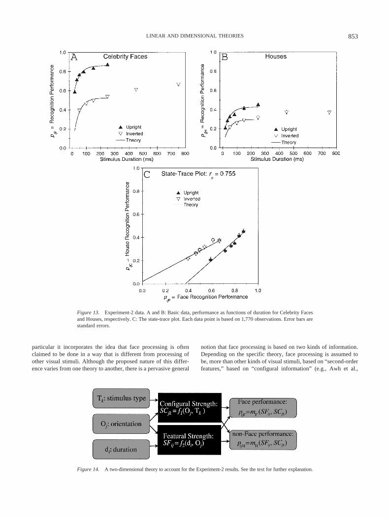
particular it incorporates the idea that face processing is oftenclaimed to be done in a way that is different from processing ofother visual stimuli. Although the proposed nature of this differ-ence varies from one theory to another, there is a pervasive general

notion that face processing is based on two kinds of information.Depending on the specific theory, face processing is assumed tobe, more than other kinds of visual stimuli, based on “second-orderfeatures,” based on “configural information” (e.g., Awh et al.,

Figure 13. Experiment-2 data. A and B: Basic data, performance as functions of duration for Celebrity Facesand Houses, respectively. C: The state-trace plot. Each data point is based on 1,770 observations. Error bars arestandard errors.

Figure 14. A two-dimensional theory to account for the Experiment-2 results. See the text for further explanation.


2004; Carey & Diamond, 1977; Collinshaw & Hole, 2000; Reed,Stone, Bozova, & Tanaka, 2003; Rhodes, 1988), based on“second-order relational information” (e.g., Diamond & Carey,1986), based on “holistic” or “gestalt” information (Farah et al.,1995; Farah, Wilson, Drain, & Tanaka, 1998; Sargent, 1984), or“carried out in parallel” (e.g., Bradshaw & Wallace, 1971). Thisprocessing mode is contrasted to featural or serial processing thatis assumed to be relatively more important in processing non-Facestimuli.

Given these considerations, we retain the notion of “Strength”but assume two Strength dimensions. The first is featural Strength(SFij), which depends only on duration (di) and orientation (Oj)The second is configural Strength (SCjk), which depends only onorientation (Oj) and stimulus type (Tk). Face and non-Face perfor-mance are determined by monotonic functions mF and mH of thesetwo kinds of Strength.

This theory is not meant to favor any one of the many proposedtheories of face processing and of the FIE that are in the literaturebut rather represents an attempt to incorporate the general idea oftwo processing modes—one relatively more important for faceprocessing—that are common to most of the theories. We recog-nize that the particular terms configural and featural are used insome theories but not others, but we note that even in the specifictheory that we present in the next section, we use the terms only assomewhat arbitrary stand-ins for what we intend to be moregeneral concepts.

A Specific Theory

The next theory-construction step was to specify the functionsf1, f2, mF, and mH (see Figure 14) such that they would producequantitative predictions. Our choice of these specifications wasbased on two considerations. First, we designed our theory to beone of a quite successful class of information-processing theories,variants of which have been described by numerous investigators(e.g., Busey & Loftus, 1994; Loftus, Busey, & Senders, 1993;Massaro, 1970; Rumelhart, 1970; Shibuya & Bundesen, 1988),that assume random sampling over time of information from avisual stimulus. Such theories imply some internal measure, forexample, “Information” or “Strength”, and/or observed perfor-mance to increase with stimulus duration by the function (1 ekd), where d is duration and k is a constant.

The second consideration driving theory design was based onthe data obtained in Experiments 1 and 2. We have already shownwhy the monotonic state-trace plot in Figure 12C and the non-monotonic state-trace plot in Figure 13C confirm a unidimensionaltheory and imply a multidimensional theory, respectively. How-ever there is additional information in these state-trace plots thatallows stronger inferences: As is apparent in Figures 12C and 13Cand as is indicated in Table 3, both the Upright and the Invertedfunctions are approximately linear. Accordingly, we decided torestrict our choice of quantitative theory to those that imply linearstate-trace functions. This decision strongly constrains our poten-tial theories.

Equations for featural Strength and configural Strength. Togenerate quantitative predictions, we specify the various functionsof the Figure-14 theory. For featural Strength SFij in durationcondition i and orientation condition j (j � {U, I}),

SFij � � �1 � edi/b� � YU for Upright stimuli�1 � edi/b� � YI for Inverted stimuli , (12)

where di is duration. The parameter b, constrained to be positive,is an exponential growth rate common to all stimuli; it may beviewed as representing a low-level characteristic of the system thatis ignorant of stimulus meaning. The parameters YU and YI, con-strained to fall between 0 and 1, reflect asymptotic featuralStrength that can differ for Upright compared to Inverted stimuli.Note that SFij must fall between 0 and 1 and can therefore betreated as a probability.

Configural Strength, SCjk for orientation j and stimulus-type k(k � {F, H}), is defined to be

SCjk � �CUk for Upright stimuliCIF � 0 for Inverted facesCIH for Inverted non-Faces

, (13)

where the Cjk are free parameters, constrained to fall between 0and 1, and therefore interpretable as probabilities. The assumptionincorporated in Equation 13 that CIF � 0 means that no informa-tion is acquired from inverted Faces. This assumption is motivatedin part by Valentine’s (1988) observation that, “. . . configuralinformation is seen as a means of encoding upright faces, butconfigural information cannot be extracted from an inverted face”(p. 480). Equation 13 also incorporates the idea that configuralStrength can be different for Upright Faces compared with Uprightnon-Faces; that is, CUF does not necessarily equal CUH. In short,featural Strength is the same for Faces and non-Faces, whereasconfigural Strength can differ in systematic ways for the twostimulus types.

Note that Equation 13 also implies that configural Strength isacquired essentially instantaneously; that is, it does not depend onstimulus exposure duration. In the limit of course, this assumptionmust be false; some time must be required to acquire any kind ofinformation from a stimulus. Realistically, this assumption be-comes more precisely that in our experiments, all the configuralStrength that will ever be acquired can be acquired from anunmasked stimulus that is as brief as 17 ms.

Performance based on independent featural-Strength andconfigural-Strength contributions. We assume, as suggested byCollinshaw and Hole (2000), that recognition can be carried out

Table 3Measures of Linearity for State-Trace Plot Functions forExperiments 1–3

Orientation Slope Intercept r2

Experiment 1

Upright 0.800 0.020 0.986Inverted 0.873 0.034 0.987

Experiment 2


Experiment 3



independently on the basis of either featural or configural Strength,and accordingly we combine them via a probability-summationrule. We also include, because our data require it, a differentperformance asymptote for Faces and non-Faces. Thus,

pijk � � �SFij � �1 � SFij�SCjF�YF for Faces�SFij � �1 � SFij�SCjH�YH for non-Faces , (14)

where the asymptotes, YK (K � {F, H}), are free parametersbetween 0 and 1.

Temporal boundary conditions. We note that this theory isonly applicable to information acquisition within a single eyefixation: At the beginning of the second and each subsequent eyefixation on a stimulus, new featural Strength would become avail-able, and the acquisition process embodied in Equation 12 wouldbegin anew. It would be possible to model this process in thepresent experiments wherein eye fixations have not been explicitlymonitored. However, such modeling would be quite cumbersome,and accordingly, we do not attempt to do so. Instead, we confineour data fit to conditions involving durations 250 ms or less. Thisprocess excludes only the two longest-duration Inverted conditionsof Experiment 2.

Outcomes that imply a unidimensional theory. If CUF and CUH

are equal and in addition CIH � CIF � 0, the theory collapses intoa unidimensional theory. The reasoning that leads to this assertionis as follows. From Equation 12, it is evident that featural Strength,SFij, is always a function only of duration (i) and orientation (j).Likewise, from Equation 13, when CUF � CUH and CIH � 0, SCjk

becomes a function only of orientation (k): For Upright stimuli, wecan define CUF � CUH � CU, whereas for Inverted stimuli, CIH �CIF � CI � 0. Thus we are left with only two states of C: CU andCI. Given these constraints, an overall measure of “Strength,”which depends only on duration, i, and orientation, j, can bederived from the bracketed portions of Equation 14 to be

Sij � SFij � �1 � SFij�Cj, (15)

where j � {U, I}. Performance is then simply

pijk � �SijYF for FacesSijYH for non-Faces . (16)

Note that Equations 15 and 16 are instances of Equations 4 and 5,respectively, which define a unidimensional theory.

State-trace plot linearity. Earlier, we noted that we con-strained our choice of theories to those that predicted linear state-trace plots. Appendix A shows that by the theory defined byEquations 12–14, the state-trace functions relating House to Faceperformance are linear with predicted slope and intercept valuesfor orientation j of

Slope j �YH�1 � CjH�

YF�1 � CjF�(17)

and

Intercept j �YH�CjH � CjF�

�1 � CjF�. (18)

Note that a zero intercept value for some orientation, j, implies that(CjH CjF) � 0 or that CjH � CjF. In particular, this must happenfor both orientation functions when the theory collapses to aunidimensional theory: Here, as described above, CUH � CUF, andCIH � CIF � 0.

Theory Fits

We first apply the theory to the Experiment-2 data and show thatit fits reasonably well. We then apply it to the Experiment-1 datawhereupon, as we demonstrate, it collapses into a unidimensionaltheory, as implied by the monotonic Experiment-1 state-trace plot.

Theory fit to Experiment 2. We fit the theory to theExperiment-2 data using a least mean-square criterion. The best-fitting values of the eight free parameters, along with fit measuresare shown in the third row of Table 4. The theoretical predictionsare shown as the smooth lines in Figure 13. As can be seen, the fitis reasonably good as shown by the relatively small root-mean-square error (0.022) and the high data-theory correlation (r2 �0.994). Accordingly, it is appropriate to interpret the estimatedparameter values in meaningful ways.

There are several noteworthy aspects of the fits. First, Uprightconfigural Strength, CUk, is greater for Faces (CUF � 0.478) thanfor Houses (CUH � 0.166). Second, Inverted configural Strength is

Table 4Theory Fits for Experiments 1–3

Experiment

Theory parameter Fit measurea

b(ms)b YU YI CUF CUH CIH YF YH

Root-mean-squareerror (df) Pearson r2

1c 45.3 0.988 0.621 0.294 0.270 0.000 0.444 0.330 0.018 (16) 0.9781d 45.3 0.838 0.551 0.253 0.253 0.000 0.502 0.371 0.018 (17) 0.9782 40.4 0.734 0.524 0.478 0.166 0.036 1.000 0.550 0.022 (12) 0.9943 46.9 0.910 0.613 0.619 0.116 0.000 0.931 0.693 0.023 (12) 0.992

Note. b � featural Strength growth rate; YU � featural Strength Upright asymptote; Y1 � featural Strength Inverted asymptote; CUF � configural Strength(Upright faces); CUH � configural Strength (Upright non-Faces); CIH � configural Strength (Inverted non-Faces); YF � performance asymptote (Faces);YH � performance asymptote (non-Faces).a Root-mean-square error is total squared theory-data deviations divided by number of data points minus number of free parameters. Pearson r2 is betweenthe predicted and observed data points over the 24 duration � orientation � stimulus type conditions. The fits in Experiments 2 and 3 exclude thelongest-duration conditions for both Faces and non-Faces; accordingly, they are based on 20 rather than 24 conditions. b A lower value implies fasterfeature acquisition rate. c CUF and CUH vary independently. d CUF and CUH are constrained to be equal.


close to zero for Houses (CIH � 0.036). We also note that featuralStrength, SFij, asymptotes at a higher level for Upright stimuli(YU � 0.734) than for Inverted stimuli (YI � 0.524), therebyimplying (unsurprisingly) that more featural Strength can be ac-quired from Upright than from Inverted stimuli.

Theory fit to Experiment 1. We fit the same theory to theExperiment-1 data. We did so in two ways. First, we allowed alleight parameters to vary freely, and second, we constrained theUpright configural-Strength values to be equal for Faces andHouses. The results are shown in the first two rows of Table 4.When the CUk’s are allowed to vary freely, they are estimated to bealmost identical (CUF � 0.294 and CUH � 0.270). When the CUk’sare constrained to be equal, the resulting estimated parametervalues change somewhat, but the fit measures are unchanged. TheInverted-House configural Strength value, CIH, was estimated tobe zero in both cases. The theory fits shown in Figure 12 are fromthe fit in which the CUk’s are constrained to be equal. It seems safeto conclude that as we inferred from the state-trace plots, a unidi-mensional version of our theory can account for the Experiment-1data (where CUF � CUH and CIH � CIF � 0) but not for theExperiment-2 data (where CUF � CUH).

Discussion: Theory Fits

Our theory fit both the Experiment-1 and the Experiment-2 dataquite well. The estimated parameter values are instructive in sev-eral ways. First, configural Strength for Inverted Faces was esti-mated to be zero or close to zero for both experiments. Thisobservation extends to Houses, Valentine’s (1988) assertion thatconfigural Strength can reasonably be construed to be zero forInverted Faces. Confirming our conclusions based on the state-trace plots, the parameter estimates indicated that two dimensions,featural Strength and configural Strength, were necessary andsufficient to account for the Experiment-2 data (CUF was estimatedto be greater than CUH), whereas in Experiment 1, the near equalityof CUF and CUH (in conjunction with CIF � CIH � 0) indicatedthat a single-dimension theory suffices to account for the data.

Experiment 3: Celebrities and Cityscapes

Experiment 2 indicated that when face retrieval is required inthe study phase of a recognition experiment, a FIE emerges.Experiment 3 was designed to extend and replicate Experiment 2under somewhat different conditions: The non-Face stimuli con-sisted of pictures of heterogeneous Cityscapes rather than thehomogeneous Houses used in Experiments 1 and 2.

We had, in particular, three goals in Experiment 3. First, asindicated, we wanted to replicate Experiment 2 and show that itgeneralizes to a stimulus class beyond Houses. Second, our quan-titative theory was developed post hoc, based in part on theExperiment-1 and Experiment-2 data patterns. Accordingly, it isdesirable to confirm that it can also fit data from a new experiment,that is, that with its eight free parameters, it was not simply fittingnoise from Experiments 1 and 2. Third, both Experiments 1 and 2indicated that within the context of our theory, configural Strengthwas zero for Houses as well as for Faces. Is configural Strengthequal to zero for inverted stimuli from any mono-oriented stimulusclass? We cannot, of course, answer this question completelywithout carrying out the impossible task of testing all such stim-

ulus classes. However, generalization to a quite different stimulusclass, Cityscapes, would strongly suggest a phenomenon that isfairly general, not specific to homogeneous stimuli such as Facesand Houses.

Method


Stimuli. A new stimulus set, Cityscapes was created. These were 144photos of skylines, individual buildings, street scenes, and bridge–waterscenes from numerous cities (excluding Seattle), all rendered as grayscaledrawings 450 pixels high and 400 pixels wide. Examples are provided inthe bottom row of Figure 11.

Apparatus. The apparatus was the same as that used in Experiments 1and 2.

Design, procedure, and counterbalancing. Procedures and counterbal-ancing measures were the same as in Experiment 2 except that only 24groups were run: In all groups, Faces were shown in the first subsession,followed by Cityscapes in the second subsession. This was an efficiencymeasure implemented because Experiments 1 and 2 indicated no stimulus-type order effects, and the additional power gained by doubling the numberof observers didn’t appear to be needed.

Results

The results are shown in Figure 15, which is organized likeFigures 12 and 13. For the three durations that are common to bothorientations, the orientation effect is greater for Faces than forCityscapes: The interaction’s mean magnitude is 0.161 � 0.028.

Figure 15C shows the state-trace plot, which like itsExperiment-2 counterpart, is nonmonotonic: The Inverted stimuluspoints are shifted leftward—that is, toward poorer Face perfor-mance—compared with the Upright stimuli. Again, we rejectunidimensional theory and conclude that there is a FIE, that is, thatinversion affects Faces more than Cityscapes.

We fit our quantitative theory to the Experiment-3 data. Thebest-fitting parameter values are shown in the fourth row of Table4, and the predictions are shown as the smooth curves through theFigure-15 data points. The fits and the parameter values are similarto those of Experiment 2.

Discussion

Experiment 3 nicely replicates Experiment 2, thereby providinganother demonstration of a FIE when face retrieval is requiredduring the study phase of a recognition experiment. The estimatedparameter values are qualitatively quite similar to those of Exper-iment 2. Of most note is that configural Strength for InvertedCityscapes is estimated to be zero, thereby adding credence to theproposition that configural Strength, whatever it is defined to be, isnot acquired from inverted stimuli in general.

General Discussion

In this article, we have developed two quite distinct themes. Thefirst focuses on a comparison between linear theory and dimen-sional theory, and the second focuses on a specific question aboutthe circumstances under which the FIE does or does not emerge.


These two themes are united by a critical observation: One canmake a decision about whether some effect, for example, a FIE,has emerged only within the context of some fundamental theory.Simulation 1 and Experiment 1 are pivotal in demonstrating theconsequences of this observation: In both, the data patterns weresuch that a FIE was inferred to have emerged if one interpreted thedata within the context of linear theory, but was inferred to havenot emerged if one interpreted the data within the context ofdimensional theory. If this kind of data pattern had been observedonly in Experiment 1, it might have been dismissed as some kindof weird statistical fluke. That the same data pattern was observedin the noise-free Simulation-1 data demonstrates that the conun-drum raised by it is real.

In what follows, we first summarize the relations between lineartheory and dimensional theory. We conclude, as we tentatively didfollowing discussion of our simulations, that dimensional theory ismore flexible and more realistic than linear theory as a context forthinking about psychological problems, for designing experiments,

and for analyzing and interpreting data. After offering these argu-ments, we turn to the FIE and summarize what we have learnedabout it.

Linear Theory and Dimensional Theory

In this section, we compare the benefits of using linear theoryversus dimensional theory as a foundation for data interpretation.

Linear Theory Is a Special Case of Dimensional Theory

Earlier we characterized dimensional theory as comprising twocomponents: a mapping from the independent variables to dimen-sional values (Equation 2) and a mapping from the dimensionalvalues to the dependent variables (Equation 3). Linear theory canbe construed as having the same structure. In the most generalcase, there are 2M 1 dimensions corresponding to the main andinteraction effects of the M independent variables. In the present

Figure 15. Experiment-3 data. A and B: Basic data, performance as functions of duration for Celebrity Facesand Cityscapes, respectively. C: The state-trace plot. Each data point is based on 960 observations. Error barsare standard errors.


case of M � 3 independent variables, there are 23 1 � 7dimensions, and we can recast Equation 1, the linear-theory rep-resentation in terms of the dimensional-theory representation ofEquations 2 and 3. Assume some condition Cijk corresponding tolevel i of IV1, level j of IV2, and level k of IV3. Then, we candenote the value of the dth dimension for Cijk as Vdijk, and theinstantiation of Equation 2 becomes

V1ijk � f1�IV1, IV2, IV3� � f1�IV1� � �i

V2ijk � f2�IV1, IV2, IV3� � f2�IV2� � �j

V3ijk � f3�IV1, IV2, IV3� � f3�IV3� � �k

V4ijk � f4�IV1, IV2, IV3� � f4�IV1, IV2� � �ij

V5ijk � f5�IV1, IV2, IV3� � f5�IV1, IV3� � �ik

V6ijk � f6�IV1, IV2, IV3� � f6�IV1, IV2� � jk

V7ijk � f7�IV1, IV2, IV3� � f7�IV1, IV2, IV3� � ijk

. (19)

The seven values then simply sum to produce a single dependentvariable for Cijk; so the instantiation of Equation 3 is

pijk � �d�1

D

Vdijk. (20)

This treatment makes it clear that Equation 19 is a special case ofEquation 2, and Equation 20 is a special case of Equation 3.Therefore, linear theory is a special case of dimensional theory.2 Itis, indeed, a special case that does not have a great deal ofpsychological validity, in that linearity is rarely a property ofpsychological processes. As we have discussed, for example, prob-ability correct is not gracefully predicted by linear processes inwhich sums of effects, unlike probabilities, are not constrained tolie between 0.0 and 1.0. It is for this reason that the simulatedprobabilities in our simulations could not themselves issue from alinear structure, which, in turn, was responsible for the chaoticbehavior of the results.

In our view, this stark demonstration of the relation betweenlinear theory and dimensional theory underscores the point that themore general and flexible dimensional theory, rather than the morespecific and inflexible linear theory, should be viewed as a startingpoint for construction of theory within psychology, or, for thatmatter, within most sciences. This point should come as no sur-prise. The literature is bespeckled with warnings about limitationsof linear theory (e.g., Loftus, 2002), particularly when interpreta-tions of nonordinal interactions are at issue (e.g., Bogartz, 1976;Loftus, 1978). The linear-theory based inconsistencies that wehave reported in conjunction with Simulations 1–3 are simplyexplicit manifestations of these limitations.

Linear theory and dimensional theory as models of the FIE. Amajor point of this article was to determine circumstances underwhich a FIE does and does not emerge. To do so requires a specificmodel of when there is no FIE, which can then be either confirmedor disconfirmed by the data. Both linear theory and dimensionaltheory offer a means way of modeling lack of a FIE: Within thecontext of linear theory, lack of FIE is specified by the absence ofan orientation � stimulus type interaction, whereas within thecontext of dimensional theory, lack of FIE is embodied in aunidimensional theory. How useful are these two models? Someinsights can be gleaned by considering the formal relations be-tween linear theory and unidimensional theory.

The specific unidimensional theory that we have consideredthroughout this article is one in which two independent variables,

duration and orientation, combine into a single measure (Strength)that then determines performance for both Faces and Houses. InAppendix B, we elaborate on the relations between linear theory,dimensional theory, and the particular unidimensional theory thatwe have considered. In Appendix B, we demonstrate that when,within the context of linear theory, there are any nonzero interac-tions involving stimulus type, linear theory is a multidimensionaltheory. The converse, as implied by the results of Appendix B andas illustrated in Simulation 3, is that when there are no interactionsinvolving stimulus type, linear theory is a unidimensional theory.This is a useful result: Confirmation of unidimensional theory, inthe form of a monotonic state-trace plot (see Figures 2, 12, andespecially 9), implies the existence of a linear structure involvingno stimulus-type interactions—which, of course, implies no FIE,even within the context of linear theory.

Suppose, in other words, that one observes a classical stimulustype � orientation interaction in the data. As we have shown, mostspecifically in Simulation 3, such an observation does not neces-sarily imply that there is an interaction in the underlying linearstructure: Any nonlinear mapping from the underlying linear struc-ture to the observed data almost certainly introduces some kind ofinteraction even if there was none there to begin with. However, anobserved monotonic state-trace plot implies that there are nounderlying interactions involving stimulus type.

Reassessing data. The foregoing is such a critical point thatwe would like to elaborate on it in the form of revisiting some ofthe data presented earlier. First, consider Simulation 3. Supposethat Simulation 3 were a real experiment, that is, that the Figure-8data were observed in real life. Again, supposing that we hadessentially infinite statistical power, we would have inferred asmall negative FIE, which is seen most directly in Figure 8D.Switching now to our actual status of the data’s creators, we knowthat the structure underlying the data, expressed in Equation 10,included no FIE and indeed no interactions at all involving stim-ulus type: It was only the nonlinear (Gaussian) measurementmapping that produced the FIE observed in the data.

However—and this is what we wish to emphasize—even if wedid not know about the underlying FIE-less linear structure tobegin with, we could have inferred it from the monotonic state-trace plot of Figure 9. Indeed, the same point holds true with theSimulation-1 data (see Figure 1). Even though the Simulation-1structure was not originally expressed as a linear structure, weknow from the monotonic state-trace plot (see Figure 2) that itcould have been expressed as a FIE-less linear structure—in fact alinear structure with no stimulus-type interaction terms at all—along with a nonlinear mapping from the structure to performance.

Finally, we can make the same inference with our realExperiment-1 data (see Figure 12). Even though, as in Simulation1, there is an observed FIE in the form of an orientation � stimulustype interaction, we can infer from the monotonic state-trace plot(see Figure 12C) that there exists an underlying FIE-less linearstructure, along with a nonlinear mapping from this structure to thedata. This is a very powerful conclusion and affords an alternativeperspective on the assertion that despite the FIE observed in thedata, there is no FIE in the underlying structure.

2 We thank John Dunn for pointing out this relation between lineartheory and dimensional theory, along with its implications.


Difficulties in Interpreting Data From Simpler Designs

The simulations and experiments in this article all involvedesigns in which stimulus duration is manipulated along with thetwo other independent variables—orientation and stimulus type—that are central in assessing the FIE. However, an investigatorembarking on a standard investigation of the FIE would normallyconsider inclusion of duration, or any other independent variable,to be superfluous. Of critical interest, from the investigator’sperspective, is the interaction between orientation and stimulustype. Thus the standard FIE investigation would entail a simple2 � 2 design in which only orientation and stimulus type aremanipulated. Such 2 � 2 designs are a staple of FIE investigationsand of psychological research in general. One might ask how thelogic that we have described—particularly the logic underlyingstate-trace plots and associated tests of dimensional theories—would apply to such simpler designs.

Scaling problems (serious ones): Comparisons of differencescores are not robust. The answer is that a 2 � 2 design isinsufficient to test theories of any complexity. The reason is this:Most scales used in psychology are generally valid only up to amonotonic transformation; that is, two potential dependent vari-ables, for example, probability and d�—or a potential dependentvariable and an internal construct, for example, probability and“Strength”—can, in general, be assumed to be only monotonicallyrelated. Therefore, differences on such scales cannot be meaning-fully compared; two differences that are, say, equal in one scale areusually unequal in some other equally valid but nonlinearly relatedscale, and vice versa. This leads directly to the difficulties ininterpretations of interactions that have been discussed in the past(e.g., Bogartz, 1976; Loftus, 1978): An interaction observed withsome particular dependent variable, for example, probability cor-rect, can disappear or even reverse when expressed either in termsof some other dependent variable or in terms of some hypotheticalinternal construct.

The virtues of equality. So, comparisons of differences areunstable across monotonic transformations. In contrast, equality ispreserved across all monotonic transformations: Two conditionsthat are equal on one scale, for example, probability, are likewiseequal on any other monotonically related scale, be it anotherdependent variable (e.g., d�) or some internal construct of interest(e.g., “Strength”). Therefore, robust conclusions follow when per-formance is equated for one pair of conditions—Upright andInverted Houses, say—and then compared for another pair ofconditions—Upright and Inverted Faces. Corresponding equalityof Upright and Inverted Faces would unequivocally imply oneconclusion, whereas corresponding inequality of Upright and In-verted Faces would unequivocally imply another conclusion.

To equate levels on a variable such as orientation, however,requires trading off with levels of some other variable, for exam-ple, duration or contrast, such that the intrinsically better level oforientation (Upright) is combined with an intrinsically worse levelof duration (short), whereas the intrinsically worse level of orien-tation (Inverted) is combined with an intrinsically better level ofduration (longer). By using multiple duration levels, state-tracecurves are mapped out such that equality of Upright and InvertedHouses can be observed over a wide range of performance levels,and relative performance for Faces can be compared across thisrange (see, e.g., Figures 2 and 5). Robust conclusions then ensue:

In the present examples, no FIE is inferred if Upright and InvertedFace performance is equal when Upright and Inverted Houseperformance is equal (see Figure 2), whereas a standard, positiveFIE is inferred when equal Upright and Inverted House perfor-mance is associated with poorer Inverted compared with UprightFace performance (see Figure 5). We note that other investigatorshave manipulated other variables to attain equality. For instance,Biederman and Tsao (1979) equated Chinese and American ob-servers on a control task in a Stroop paradigm by eliminating fastAmerican observers and slow Chinese observers.

Impoverished information with 2 � 2 designs. Another way ofconceptualizing the difficulty in interpreting standard 2 � 2 de-signs is by reference to Figure 1D. Assuming a 2 � 2 design, theexposure duration would have to be selected to have been some-thing, and the observed magnitude of the FIE would then dependon which particular duration value had been selected. As is evidentin Figure 2D, the observed FIE would have been observed to be nilhad the selected duration been less than about 100 ms and wouldhave been greater with greater selected durations. As if this werenot bad enough, even these conclusions are tenuous because as isapparent in Figure 3, even the relation between duration and FIEmagnitude is not very robust.

Nested Dimensional Theories

We now turn to a brief review of the usefulness of thinking interms of dimensional theories. The complex designs of Simula-tions 1–3 and Experiments 1–3 have guided the construction ofthree nested dimensional theories—that is, theories devised suchthat each successive theory is a special case of the precedingone—within whose context we have sought to understand theresults of our experiments. In what follows, we summarize howthese theories provide an increasingly specific understanding ofthe nature of the FIE. In the present experiments, these theorieswere used to investigate whether the FIE is characteristic ofstorage of face information and/or retrieval of face information;however, the theories, or variants of them, could be used to assessany question about face processing, the FIE, and the circumstancesunder which the FIE does or does not emerge.

Theory I: Generic Dimensional Theory

Theory I, the most general, is generic dimensional theory (Equa-tions 2 and 3), wherein we simply assume that the independentvariables in our experiments result in some number of internaldimensions, the values of which then determine performance. Likegeneric linear theory, Theory I is not in and of itself particularlyuseful in understanding the FIE or any other process; it simplyprovides a theoretical shell within which more specific theoriesmay be formulated.

Theory II: Configural and Featural Strength

We deem that actual insight into the nature of the FIE beginswith Theory II: the two-dimensional theory presented in Figure 14.Here, we identify constructs that have been used in the past toexplain face processing in general and the FIE in particular.Specifically, we postulated two kinds of Strength—drawn frommany past accounts of face processing—that are assumed to accrue


during inspection of a visual stimulus. In this incarnation of thetheory, we assume that featural Strength accrues over time in amanner that is indifferent to the nature of the stimulus but never-theless depends on stimulus duration and stimulus orientation.Configural Strength is, in keeping with the notion of face-processing “specialness,” allowed to be different for Faces andnon-Faces as well as for different orientations.

Theory III: A Quantitative Version of Theory II

In Theory III, we fleshed out these assumptions with specificfunctions that allowed quantitative fits to the data from our threereal experiments. Our decisions about exactly how to structure thisstrong version of the theory were somewhat but not entirelyarbitrary: As noted, they were constrained by the nature of pastquantitative visual-information-acquisition theories and indepen-dently by the observed approximately linear forms of the Experi-ments 1–3 state-trace plot functions. The theory fits to the data setswere quite good (see Figures 12, 13, and 15), and the estimatedparameter values (see Table 4) therefore constitute a useful tool forinterpreting the subtle and complex language spoken by the data.

Face Recognition and the FIE

Experiments 1–3 were designed to assess Valentine’s (1988)assertion that a FIE does not emerge when orientation is manipu-lated in the study phase of a visual-recognition experiment. Whatcan we conclude about this issue?

In our experiments, we manipulated orientation only during thestudy phase of a visual-recognition procedure: A FIE did notemerge when unfamiliar computer-generated Faces were com-pared with Houses (Experiment 1), but a FIE did emerge whenphotographs of familiar (celebrity) Faces were compared withHouses (Experiment 2) or Cityscapes (Experiment 3). This findingis consistent with the proposition that the FIE emerges whenfamiliar faces are retrieved from memory, as almost certainlyhappens during the study phase of Experiments 2 and 3, but doesnot emerge when unfamiliar faces are encoded for subsequentrecognition, as must happen during the study phase of Experiment1. Such a proposition is reasonable given the findings that pro-cessing of familiar faces differs in many respects from processingof unfamiliar faces (see, e.g., Bruce, Henderson, Newman, &Burton, 2001; Hancock, Bruce, & Burton, 2000).

However, this conclusion must be tempered by (at least) twocaveats. First, this pattern of results may not be unique to faces but,rather, may characterize any stimulus set that can occur in afamiliar or an unfamiliar configuration. An example is buildings,which, like faces, come in unfamiliar versions (i.e., most build-ings) and familiar versions (e.g., the Empire State Building, the TajMahal, etc.). Although, to our knowledge, the experiment has notbeen done, it seems perfectly plausible that a “building-inversioneffect” would emerge when familiar but not unfamiliar buildingsare compared with a uniform set of unfamiliar stimuli, such ashouses.

The second caveat is that as is evident from even a quick glanceat Figure 11, the computer-generated faces used in Experiment 1,though guaranteed to be unfamiliar, differ in many respects fromthe celebrity faces used in Experiments 2 and 3. Possibly ourobservers were not treating these computer-generated faces as

actual faces, and that is why they didn’t differ from houses withrespect to the inversion effect. Numerous research projects suggestthemselves to test this possibility.

On the Prevalence of the FIE

In the introduction to this article, we provided numerous refer-ences to reports of a FIE measured by the traditional stimulustype � orientation interaction. Generally speaking, these findingsappear to have formed a robust and reasonably harmonious patternthat has assisted us in understanding face processing. Are wesuggesting that because of the interpretational difficulties impliedby Simulations 1–3, these findings simply be declared invalid untilthey are reinvestigated within the context of dimensional theory?And where, by the way, are all those negative FIE’s whoseexistence is suggested by the chaotic demonstrations illustrated inFigures 3, 6, and 10?

These questions do not have obvious answers. We do, however,make a general observation, which is that the greater the magni-tude of the FIE as characterized by the traditional interaction, theless likely that it will be associated with a lack of a FIE asdemonstrated by confirmation of a unidimensional theory: Notethat the Experiment-1 data involved quite a small-magnitude in-teraction, whereas the data from Experiments 2 and 3 involvedmuch larger-magnitude interactions. As for the lack of negativeFIE’s in the literature, there are (at least) two plausible explana-tions. The first is that we have made faulty assumptions—perhaps,unlike our simulation parameters, the structural parameters thatgovern real-life FIE data are constrained in such a way as to notallow negative FIE’s. The second explanation rests on the “file-drawer problem” (Rosenthal, 1979): Given no a priori reason toexpect a negative FIE, it is unlikely that anyone who obtained sucha result would publish it.

Conclusions

In this article, we have tried to make two main points. The first,which in our view is the less important, has to do with the FIE: Wehave provided evidence suggesting that a FIE emerges whenknown faces are retrieved from memory but not when unknownfaces are encoded in memory. Although consistent with priorconjectures, our data are nevertheless subject to a number ofalternative interpretations and should thus be viewed as a startingpoint for future research projects rather than as grounds for unam-biguous conclusions about the nature of face processing.

The second point, which we consider the more important, isquite radical: We have asserted and have tried to demonstrate thatstandard, off-the-shelf linear theory is highly limited in its useful-ness as a foundation for conceptualizing psychological problemsand analyzing psychological data. We have described an alterna-tive, dimensional theory, which as we have shown, subsumeslinear theory: Dimensional theory is more general both in terms ofthe functions mapping independent variables to presumed internalconstructs and in terms of the functions mapping the presumedinternal constructs to the observed dependent variables.

As we have indicated, tests of specific dimensional theoriesgenerally require relatively complex designs; the standard 2 � 2,for example, is generally inadequate. We are convinced, however,that such complex experiments, carried out in conjunction with


carefully specified dimensional theories, will bear fruit in the formof deeper and more robust understandings of all manner of psy-chological phenomena.

References

Anderson, N. H. (1974). Information integration theory: A brief survey. InD. Krantz, R. C. Atkinson, D. Luce, & P. Suppes (Eds.), Contemporarydevelopments in mathematical psychology (Vol. 2., pp. 236–305). NewYork: Freeman.

Anderson, N. H. (1979). Algebraic rules in psychological measurement.American Scientist, 67, 555–563.

Anderson, N. H. (1981). Foundations of information integration theory.New York: Academic Press.

Awh, E., Serences, J., Laurey, P., Dhaliwal, H., van der Jagt, T., &Dassonville, P. (2004). Evidence against a central bottleneck during theattentional blink: Multiple channels for configural and featural process-ing. Cognitive Psychology, 48, 95–126.

Bamber, D. (1979). State trace analysis: A method of testing simpletheories of causation. Journal of Mathematical Psychology, 19, 137–181.

Biederman, I., & Tsao, Y. C. (1979). On processing Chinese ideographsand English words: Some implications from Stroop task results. Cogni-tive Psychology, 11, 125–132.

Bogartz, R. S. (1976). On the meaning of statistical interactions. Journal ofExperimental Child Psychology, 22, 178–183.

Bradshaw, J. L., Taylor, M. J., Patterson, K., & Nettleton, N. C. (1980).Upright and inverted faces, and housefronts in two visual fields. Journalof Clinical Neuropsychology, 2, 245–257.

Bradshaw, J. L., & Wallace, G. (1971). Models for the processing andidentification of faces. Perception & Psychophysics, 9, 443–448.

Brainard, D. H. (1997). The Psychophysics Toolbox. Spatial Vision, 10,433–436.

Bruce, V., Henderson, Z., Newman, C., & Burton, A. M. (2001). Matchingidentities of familiar and unfamiliar faces caught on CCTV images.Journal of Experimental Psychology: Applied, 7, 207–218.

Bruyer, R., & Velge, V. (1981). Lesions cerebrale unilateral et troubledirect examination la perception des visage: Specificite du deficit? ActaNeurological Belgica, 81, 321–332.

Busemeyer, J. R., & Jones, L. E. (1983). Analysis of multiplicative com-bination rules when the causal variables are measured with error. Psy-chological Bulletin, 88, 237–244.

Busey, T. A., & Loftus, G. R. (1994). Sensory and cognitive componentsof visual information acquisition. Psychological Review, 101, 446–469.

Busey, T. A., Tunnicliff, J., Loftus, G. R., & Loftus, E. F. (2000). Accountsof the confidence-accuracy relation in recognition memory. Psy-chonomic Bulletin & Review, 7, 26–48.

Carey, S., & Diamond, R. (1977, January 21). From piecemeal to config-ural representation of faces. Science, 195, 312–314.

Collinshaw, S. M., & Hole, G. J. (2000). Featural and configural processesin the recognition of faces of different familiarity. Perception, 29,893–909.

Coltheart, M. (1985). Cognitive neuropsychology and the study of reading.In M. I. Posner & O. S. M. Marin (Eds.), Attention & performance XI(pp. 3–37). Hillsdale, NJ: Erlbaum.

Diamond, R., & Carey, S. (1986). Why faces are and are not special: Aneffect of expertise. Journal of Experimental Psychology: General, 115,107–117.

Dunn, J. C., & James, R. N. (2003). Signed difference analysis: Theory andapplication. Journal of Mathematical Psychology, 47, 389–416.

Dunn, J. C., & Kirsner, K. (1988). Discovering functionally independentmental processes: The principle of reversed association. PsychologicalReview, 95, 91–101.

Ellis, H. D., & Shepherd, J. W. (1975). Recognition of upright and invertedfaces presented in the left and right visual fields. Cortex, 11, 3–7.

Farah, M. J., Tanaka, J. N., & Drain, M. (1995). What causes the faceinversion effect? Journal of Experimental Psychology: Human Percep-tion and Performance, 21, 628–634.

Farah, M. J., Wilson, K. D., Drain, M., & Tanaka, J. N. (1998). What is“special” about face perception? Psychological Review, 105, 482–498.

Garner, W. R. (1974). The processing of structure and information. NewYork: Wiley.

Gauthier, I., Curran, T., Curby, K. M., & Collins, D. (2003). Perceptualinterference supports a non-modular account of face processing. NatureNeuroscience, 6, 428–432.

Hancock, P. J. B., Bruce, V., & Burton, A. M. (2000). Recognition ofunfamiliar faces. Trends in Cognitive Science, 4, 330–337.

Harley, E. M., Dillon, A., & Loftus, G. R. (2004). Why is it difficult to seein the fog? How contrast affects visual perception and visual memory.Psychonomic Bulletin & Review, 11, 197-231.

Hays, W. (1973). Statistics for the social sciences (2nd ed.). New York:Holt.

Kanwisher, N., McDermott, J., & Chun, M. M. (1997). The fusiform facearea: A module in human extrastriate cortex specialized for face per-ception. Journal of Neuroscience, 17, 4302–4311.

Kanwisher, N., Tong, F., & Nakayama, K. (1998). The effect of faceinversion on the human fusiform face area. Cognition, 68, B1–B11.

Krantz, D. H., Luce, R. D., Suppes, P., & Tversky, A. (1971). Foundationsof measurement. New York: Academic Press.

Krantz, D. H., & Tversky, A. (1971). Conjoint measurement analysis ofcomposition rules in psychology. Psychological Review, 78, 151–169.

Kruskal, J. B. (1964). Multidimensional scaling: A numerical method.Psychometrica, 29, 115–129.

Leehey, S., Carey, S., Diamond, R., & Cahn, A. (1978). Upright andinverted faces: The right hemisphere knows the difference. Cortex, 14,411–419.

Loftus, G. R. (1978). On interpretation of interactions. Memory & Cogni-tion, 6, 312–319.

Loftus, G. R. (1985). Evaluating forgetting curves. Journal of Experimen-tal Psychology: Learning, Memory, and Cognition, 11, 396–405.

Loftus, G. R. (2002). Analysis, interpretation, and visual presentation ofdata. In H. Pashler (Ed.) & J. Wixted (Vol. Ed.), Stevens’ handbook ofexperimental psychology (3rd ed., Vol. 4, pp. 339–390). New York:Wiley.

Loftus, G. R., & Bamber, D. (1990). Learning–forgetting independence:Unidimensional memory models and feature models: Comment on Bo-gartz (1990). Journal of Experimental Psychology: Learning, Memory,and Cognition, 16, 916–926.

Loftus, G. R., Busey, T. A., & Senders, J. W. (1993). Providing a sensorybasis for models of visual information acquisition. Perception & Psy-chophysics, 54, 535–554.

Loftus, G. R., & Irwin, D. E. (1998). On the relations among differentmeasures of visible and informational persistence. Cognitive Psychol-ogy, 35, 135–199.

Massaro, D. W. (1970). Perceptual processes and forgetting in memorytasks. Psychological Review, 77, 557–567.

Palmer, J. C. (1986a). Mechanisms of displacement discrimination with avisual reference. Vision Research, 26, 1939–1947.

Palmer, J. C. (1986b). Mechanisms of displacement discrimination withand without perceived movement. Journal of Experimental Psychology:Human Perception and Performance, 12, 411–421.

Pelli, D. G. (1997). The videotoolbox software for visual psychophysics:Transforming numbers into movies. Spatial Vision, 10, 437–442.

Phelps, M. T., & Roberts, W. A. (1994). Memory for pictures of uprightand inverted primate faces in humans (Homo sapiens), squirrel monkeys(Saimiri sciureus), and pigeons (Columba livia). Journal of ComparativePsychology, 108, 114–125.

Phillips, R. J., & Rawles, R. E. (1979). Recognition of upright and invertedfaces: A correlational study. Perception, 8, 577–583.


Pinker, S. (1997). How the mind works. New York: Norton.Reed, C. L., Stone, V. E., Bozova, S., & Tanaka, J. (2003). The body-

inversion effect. Psychological Science, 14, 302–308.Rhodes, G. (1988). Looking at faces: First-order and second-order features

as determinants of facial appearance. Perception, 17, 43–63.Rosenthal, R. (1979). The file drawer problem and tolerance for null

results. Psychological Bulletin, 86, 638–641.Rumelhart, D. E. (1970). A multicomponent theory of the perception of

briefly exposed visual displays. Journal of Mathematical Psychology, 7,191–218.

Sargent, J. (1984). An investigation into component and configural pro-cesses underlying face perception. British Journal of Psychology, 75,221–242.

Shepard, R. N. (1962). The analysis of proximities: Multidimensionalscaling with an unknown distance function. Psychometrica, 27, 125–140.

Shibuya, H., & Bundesen, C. (1988). Visual selection from multielementdisplays: Measuring and modeling effects of exposure duration. Journalof Experimental Psychology: Human Perception and Performance, 14,591–600.

Tversky, A., & Russo, J. E. (1969). Substitutability and similarity in binarychoices. Journal of Mathematical Psychology, 6, 1–12.

Valentine, T. (1988). Upside-down faces: A review of the effect of inver-sion upon face recognition. British Journal of Psychology, 79, 471–491.

Valentine, T., & Bruce, V. (1986). The effect of race, inversion andencoding activity upon face recognition. Acta Psychologica, 61, 259–273.

Yin, R. K. (1969). Looking at upside-down faces. Journal of ExperimentalPsychology, 81, 141–145.

Yin, R. K. (1970). Face recognition by brain-injured patients: A dissociableability? Neuropsychologia, 8, 395–402.

Appendix A

Slopes and Intercepts of the Linear State-Trace Plots Implied by Equations 12–14

This appendix concerns the quantitative theory specified by Text Equa-tions 12–14. Our goals are (a) to prove that by this theory, the Upright andInverted state-trace functions relating House performance to Face perfor-mance are linear and (b) to derive the slopes and intercepts of thesefunctions. We prove linearity by deriving the expression for the slope anddemonstrating that slope does not depend on duration.

Assume two duration values, d1 and d2 � d1. Text Equation 14 providespredicted performance,

pijk � �SFij � �1 � SFij�Cjk�Yk � YkSFij�1 � Cjk� � YkCk, (A1)

where, as usual, j � {U, I} and k � {F, H}. Here i is restricted to i � {1,2} for the two durations under consideration. Note that SFij and Cjk areobtained from Text Equations 12 and 13.

The slope is the ratio ( p2jH p1jH)/( p2jF p1jF). Substituting the rightside of Equation 1 for the pijks,

Slope ��YHSF2j�1 � CjH� � YHCjH� � �YHSF1j�1 � CjH� � YHCjH�

�YFSF2j�1 � CjF� � YFCjF� � �YFSF1j�1 � CjF� � YFCjF�

�YH�1 � CjH��SF2j � SF1j�

YF�1 � CjF��SF2j � SF1j�

or

Slope �YH�1 � CjH�

YF�1 � CjF�, (A2)

which is the expression indicated in the text. Because the Equation A2expression for slope contains no terms involving di—it depends only onparameters relevant to orientation, j, and stimulus type, k—the slope will bethe same no matter what values of d1 and d2 are chosen, and the state-tracefunctions must therefore be linear for both orientation values.

The intercept may be derived by picking performance values for Houses,pijH, and Faces, pijF, and noting that because the functions are linear,

Intercept � pijH � Slope � pijF; (A3)

or, substituting Equations A1 and A2 into Equation A3,

Intercept � �YHSFij�1 � CjH� � YHCjH�

�YH�1 � CjH�

YF�1 � CjF�� YFSFij�1 � CjF� � YFCjF�

� �YHSFij�1 � CjH� � YHCjH� � YHCjH]

�YH�1CjH�YFSFij�1CjF�

YF�1CjF��YH�1jH�CjFYF

YF�1CjF��

� �YHSFij�1 � CjH� � YHCjH� � YHSFij�1 � CjH�

�YH�1 � CjH�CjF

�1 � CjF��

� YHCjH �YHCjF�1 � CjH�

�1 � CjF�

��1 � CjF�YHCjH � YHCjF�1 � CjH�

�1 � CjF�;

or, finally,

Intercept �YH�CjF � CjH�

�1 � CjF�,

which is the expression for intercept indicated in the text.


Appendix B

On the Relations Between Linear Theory and Dimensional Theory

Our goal here is to define relations between linear theory and dimen-sional theory. For convenience, we again assume no statistical error.

Linear theory is defined by

pijk � � � �i � �j � �k � jk � �ij � �ik � ijk, (B1)

where i, j, and k index duration, orientation, and stimulus type,respectively.

To define unidimensional theory, we slightly rewrite Text Equation 4 toobtain Strength, Sij, in duration � orientation condition ij,

Sij � f�di, Oj�, (B2)

and we similarly rewrite Text Equation 5 to obtain performance,

pijk � mk�Sij�, (B3)

where k � {F, H}. Thus, performance depends on both Strength, Sij, andstimulus type as instantiated in the two monotonic functions, mk.

We now attempt to recast linear theory as a unidimensional theory. Wefirst define Strength to be

Sij � � � �i � �j � �ij. (B4)

Thus Strength defined by linear theory (Equation B4) is a special case ofStrength defined by unidimensional theory (Equation B2). To predictperformance, we substitute Equation 4 into Equation B1 to obtain

pijk � Sij � �k � jk � �ik � ijk � mk�Sij, di, Oj�. (B5)

By Equation B5, therefore, performance depends not only on Strength, Sij,and stimulus type, �k, but also on jk, �ik, and ijk, that is, on duration andorientation. Therefore, unless jk, �ik, and ijk are all zero, linear theorycannot be a unidimensional theory; it must be multidimensional.

In the most general case in which all interaction terms are nonzero, lineartheory is a three-dimensional theory. We define the first dimension,Strength, by Equation B4. Two additional dimensions, which we call F andH both depend only on duration and orientation. They are defined as

Fij � j1 � �i1 � ij1 (B6)

and

Hij � j2 � �i2 � ij2. (B7)

Thus, F is determined only by terms relevant when faces are shown (k �1), and H is determined only by terms relevant when houses are shown(k � 2). Finally, there are separate performance equations for faces andhouses:

Faces: pij1 � Sij � Fij (B8)

and

Houses: pij2 � Sij � Hij. (B9)

Received January 14, 2004Revision received March 17, 2004

Accepted March 17, 2004 �

New Editor Appointed for History of Psychology

The American Psychological Association announces the appointment of James H. Capshew, PhD,as editor of History of Psychology for a 4-year term (2006–2009).

As of January 1, 2005, manuscripts should be submitted electronically via the journal’s ManuscriptSubmission Portal (www.apa.org/journals/hop.html). Authors who are unable to do so shouldcorrespond with the editor’s office about alternatives:

James H. Capshew, PhDAssociate Professor and Director of Graduate StudiesDepartment of History and Philosophy of ScienceGoodbody Hall 130Indiana University, Bloomington, IN 47405

Manuscript submission patterns make the precise date of completion of the 2005 volume uncertain.The current editor, Michael M. Sokal, PhD, will receive and consider manuscripts throughDecember 31, 2004. Should the 2005 volume be completed before that date, manuscripts will beredirected to the new editor for consideration in the 2006 volume.


Linear Theory, Dimensional Theory, and the Face-Inversion Effect

Documents

Transcript of Linear Theory, Dimensional Theory, and the Face-Inversion Effect