LINEAR STATE MODELS FOR VOLATILITY ESTIMATION AND PREDICTION

A thesis submitted for the degree of Doctor of Philosophy

by

Richard Nathanael Hawkes

Department of Mathematics, Brunel University

July 2007

Brunel University, Uxbridge; Mathematics; Richard Nathanael Hawkes; Linear state models for volatility estimation and prediction; 2007; Doctor of Philosophy

Abstract

This thesis concerns the calibration and estimation of linear state models for forecasting stock

return volatility. In the first two chapters I present aspects of financial modelling theory and

practice that are of particular relevance to the theme of this present work. In addition to this I

review the literature concerning these aspects with a particular emphasis on the area of dynamic volatility models. These chapters set the scene and lay the foundations for

subsequent empirical work and are a contribution in themselves. The structure of the models

employed in the application chapters 4,5 and 6 is the state-space structure, or alternatively the

models are known as unobserved components models. In the literature these models have

been applied in the estimation of volatility, both for high frequency and low frequency data.

As opposed to what has been carried out in the literature I propose the use of these models

with Gaussian components. I suggest the implementation of these for high frequency data for

short and medium term forecasting. I then demonstrate the calibration of these models and

compare medium term forecasting performance for different forecasting methods and model

variations as well as that of GARCH and constant volatility models. I then introduce implied

volatility measurements leading to two-state models and verify whether this derivative-based

information improves forecasting performance. In chapter 6I compare different unobserved

components models' specification and forecasting performance. The appendices contain the

extensive workings of the parameter estimates' standard error calculations.

Contents

Abstract i

Table of Contents ii

List of tables v

1 Introduction I

1.1 Financial modelling ... ........................... 3

2 Modelling and statistical preliminaries S

2.1 System identification ... ................... " ..... ". 8

2.2 Model validation ................................ 9

2.3 Information and probabilistic modelling . .................. 11

2.4 The information set ............... ............... 14

2.5 Brownian motion and stochastic integration ........ ....... .. 15

2.6 Ornstein-Uhlenbeck processes ....... ............. ..... 19

2.7 Maximum likelihood estimation ........................ 21

2.7.1 Generalised Method of Moments .......... ......... 23

2.8 State-space formulation and the Kalman filter ....... ......... 23

3 Modelling volatility: estimation and forecasting 29

3.1 Dynamic volatility models .................. ......... 29

3.1.1 Stochastic volatility models .................. .... 31

3.1.2 GARCIA models .............. ..... ...... ... 33

3.1.3 Jump-diffusion models ......................... 36

3.1.4 Other dynamic volatility models .............. ..... 38

3.2 Realised volatility and high frequency data ...... ........... 39

ii

3.3 Return-based estimation techniques for stochastic volatility models .... 42

3.4 Multivariate volatility models . .... ......... ...... ..... 44

3.5 Option pricing and implied volatility ..... ..... .... ....... 45

4 Medium-term horizon volatility forecasting in practice: a comparative

study 51

4.1 Introduction ................................... 51

4.2 Linear state-space formulation ......................... 53

4.3 The calibration procedure for UC-RV models ..... .... ....... 58

4.4 GARCH model specification and calibration ........ ...... ... 59

4.5 Medium-term horizon forecasting: implementation and comparison study 61

4.5.1 The data ... ...................... ....... 63

4.5.2 Realised volatility estimation ....... ......... ..... 64

4.5.3 Parameter estimates and standard errors of UC-RV and GARCH-

type models ............. .... .............. 67

4.5.4 Comparison study ......... .................. 71

4.6 Conclusion ................................ ... 74

5 Medium-term horizon forecasting for UC-RV models with implied volatil-

ity 76

5.1 Implied volatility estimation .......................... 78

5.2 Model formulation .... .................... .... ... 82

5.2.1 Model estimation and calibration ................... 84

5.3 Conclusion ...... ........... ......... .... ..... 87

6 UC-RV model specification and model comparison 89

6.1 Introduction ................................... 89

6.2 Model presentation ....... ........ ...... .......... 90

6.3 Numerical results .................. ....... ....... 93

6.4 Conclusion ..................... .............. 98

Contributions and further work 99

Notation 101

iii

Appendix A

Appendix B

Acknowledgements

Bibliography

102

105

107

108

iv

List of Tables

4.1 Descriptive statistics for the daily return and RV series of data set 1. ... 67

4.2 Parameter estimates and standard errors for IBM for the UC-RV-type

models .......................... ............ 69

4.3 Parameter estimates and standard errors for Citigroup for the UC-RV-type

models . ....................... ... ........... 70

4.4 Parameter estimates and standard errors for the GARCH-type models .. 70

4.5 Loss function values for IBM using UC-RV-type models. .......... 72

4.6 Loss function values for Citigroup using UC-RV-type models. .... ... 72

4.7 Loss function values using constant volatility methods..... .... ... 73

4.8 Loss function values using GARCH-type models ............... 73

5.1 Descriptive statistics for the RV series of data set 2 and the IV series. .. 82

5.2 Parameter estimates and standard errors for UC-RV-IV. .......... 85

5.3 Loss function values using UC-RV-type models ......... .... ... 86

6.1 Parameter estimates and standard errors for IBM for the UC-RV-type

models . ..................................... 93

6.2 Parameter estimates and standard errors for Citigroup for the UC-RV-type

models . .... .... ...................... .... ... 94

6.3 Comparison of likelihood values for UC-RV-type models........ ... 95

6.4 Comparison of loss functions for UC-RV-type models. .... .... ... 97

B. 1 Programs for the UC-RV and GARCH-type models ...... ....... 105

V

Chapter 1

Introduction

In finance and business it is clear that uncertainty is ever present. The introduction of

preventive measures generally does not obliterate this uncertainty although it may help

to mitigate it. What remains must at least be quantified if possible. Quantified uncer-

tainty is denominated risk. The concept of volatility is related to risk in the sense that

it is an uncertain quantity. Volatility is not equivalent to risk since it is not known with

certainty neither in the past nor in the future. Risk however is quantified uncertainty in

a forward looking sense. More formally by the volatility of an asset we mean a measure

of the accumulative infinitesimal change in value of the asset over some time-interval.

This is an unobservable quantity but a natural proxy is the return variance. Clearly the

change in value of an asset can either be to our advantage or disadvantage.

The main thrust of this thesis is that of modelling volatility, which will include both es-

timation and forecasting. Modelling volatility can take on two distinct forms: parametric

and non-parametric modelling. In the first, a model is assumed in terms of an equation

or set of equations that are assumed to describe the quantity being modelled in terms of a

parameter set. In the second, the quantity of interest is estimated from the data using a

variety of statistical techniques that do not assume a parameterised form. It is of pivotal

interest to model an asset's expected future volatility for a number of reasons. Perhaps

the foremost of these is that many financial derivatives on a given asset are dependent

on the asset's future payoff, i. e. a function of its expected future rate of return. But

as this quantity is dependent on the (return) volatility this must also be estimated if a

1

derivative is to be priced'. Thus forecasting volatility is of primordial interest in this

setting alone. But volatility estimation and forecasting in financial modelling concerns

not only derivatives but also:

- Interest rate theory. Interest rate models are often composed of a term for the

volatility of the market.

- Private investments. For example, the holder of a stock is interested to estimate

the future volatility of the stock in deciding whether or not to keep the stock in

his/her portfolio.

- Capital-asset pricing. The Capital-Asset Pricing Model (CAPM), to be described

in the following section, involves the return variance of assets that are priced.

- Value-at-risk (VaR) estimation. In essence VaR is defined as the amount of loss in a

portfolio for worst-case scenarios. Clearly by very definition, this will be dependent

on the portfolio's expected future volatility. As such a volatility forecast of each

asset and/or a basket of assets must be produced. The present work will focus on

volatility forecasting for the application of VaR estimation.

The forecasting volatility literature has known a rapid increase in recent years and even

to present the major works would be a mammoth task. I do not attempt to do this.

Instead I refer to several reviews of this literature that I hope the reader will find to

compliment each other. In no particular order of importance there are the reviews of

Poon and Granger (2003), Figlewski (1997) and the introduction of Shephard (2005).

Much of the literature is also summarised in the section on dynamic volatility models 3.1

and I will defer the presentation of relevant research to this section.

In this thesis I will estimate volatility using both spot and option prices but I will be

more interested in the forecasting performance of different models than comparing volatil-

ity estimates. To this end I concentrate the empirical work on the estimation of linear

state-space models. I take the approach of estimating volatility over regularly spaced

intervals and as such a time series of volatility measurements is produced. As has been

mentioned, volatility is an unobservable quantity and is therefore measured in noise. The 'There is also the field of derivatives on volatility such as volatility swaps.

2

state-space formulation2 provides a modelling structure where measurement error from a

time series can be filtered out while at the same time the dynamics of the unobservable

process can be described. The Kalman filter, Kalman (1960) and Kalman and Bucy

(1961), is a filtering procedure that is often used in conjunction with other modelling

techniques to allow the estimation of the particular state-space formulation. More will

be said on this both in a section on the state-space formulation and the Kalman filter

as well as in the empirical applications. For now interested readers are referred to the

textbook treatment of Durbin and Koopman (2001).

There is much to be said on volatility estimation and forecasting but this will be also left

to subsequent discussions. First some background to financial modelling more generally

will be given.

1.1 Financial modelling

This section is a summary of the descriptions given in Howison et al. (1995), (Eatwell

et al., 1994, chapter 1) and Milne (1995). Readers are referred to these books for a more

detailed presentation.

We can trace the beginning of financial theory back to the Bachelier (1900) dissertation

on speculation. This work marks both the origin of the continuous-time mathematics

of stochastic problems and the continuous-time economics of option pricing. With re-

spect to the latter, Bachelier presented two different derivations of the Fourier partial

differential equation as the equation for the probability distribution of what we now call

Brownian motion. But it was not until the late 1950's that modern financial theory

began; before then the focus was mainly on the time value of money. To mark the be-

ginning of the period of modern financial theory we have the work of Markowitz (1952),

which was ground-breaking. The topic of this work, mean-variance analysis, has since

been investigated in depth and has become the standard way of approaching portfolio

optimization by practitioners'. The issue of the trade off between profit and risk is sem- 'Another name for these models is unobserved components models and it is this term that will be

employed more frequently. 3The theory introduced by Markowitz was applicable to one time period but the theory has been since

3

final but it is the latter that is most often modelled. One reason for this is that the risk factor dominates the expected returns. Another is that the variance of returns is highly

predictable whereas the returns themselves are not. Perhaps the first paper to present

empirical evidence along these lines by Kendall (1953) was highly controversial and led

to a great deal of subsequent discussion.

A couple of years later Modigliani and Miller (1958) produced an ever-since controver-

sial paper that suggested that a firm's value was independent of financing decisions. The

intuition behind this concept is that the market is well balanced so that whether the firm

borrows from a bank, sells company shares or reinvests prior earnings to finance itself,

this all amounts to the same in terms of how much capital is generated. The arguments

involved correspond to the assumption of absence of financial arbitrage in the market,

i. e. opportunities to make a riskless profit are non-existent. This concept is key and is

one of the building blocks of much of the subsequent theory on financial valuation.

Building on Markowitz, Sharpe (1964), Lintner (1965) and Mossin (1966) introduced

CAPM which later became so key in measuring the performance of investments. The

idea behind this model is that each component of a portfolio of assets is associated with a

value of non-diversifiable risk. This value proceeds from calculating an asset's covariance

with the market which is denoted the ß of the asset. During the same decade one of the

major building blocks of economic theory - the efficient market theory - was introduced

by Samuelson (1965), Roberts (1967) and Fama (1970). This theory is based upon the

conjecture that all available information is made use of in the market's valuation of as-

sets. Following this line of thought the market price will be the fair price and the market

is `arbitrage free'. Furthermore the pricing of assets is straightforward: in an efficient

market the efficient market hypothesis can be used to price assets. This hypothesis states

that the future price of an asset is the current price adjusted for a `fair' expected rate

of return. The late 1960's and the 1970's saw an advance in the development of finan-

cial models involving dynamic asset allocation and choice under uncertainty. It should

be noted that for the kinds of models being developed during this period, the partial

and stochastic differential equations and integral equations governing these models were

then extended to multi-period, cf. Mossin (1968), Samuelson (1969) and Hakansson (1971).

4

much more complex than had been worked with before in this field. While CAPM was

extended to inter-temporal valuation, Merton (1973a), evidence was given to a great deal

of limitations in the CAPM framework, Roll (1977). But before this paper Ross (1976)

introduced the arbitrage-pricing theory (APT) model, which can be viewed as a gener-

alised competitor to CAPM. The APT model is potentially more flexible and robust than

CAPM and may lead to more reliable prediction.

The well known Black and Scholes (B-S) model was introduced by Black and Scholes

(1973) and Merton (1973b). This model revolutionised the financial research and practice

of the time. The reason for this was that this model makes precise, in a straightforward

manner4, the way in which to price European options. The main idea behind the model

formulation is that for a given stock, a dynamic trading strategy can be found which will

replicate the returns of an option on that stock. Hence the fair price for the option is the

value of the replicating strategy. This is indicative of a key concept to finance, namely

that assets with the same expected payoff and risk should have the same price. Pricing

theory thus essentially consists of choosing and replicating a pricing basis. For consis-

tency this choice must be independent of risk preferences and as such we fall within the

scope of risk-neutral pricing. A risk-neutral measure is a probability measure associated

with risk-neutral pricing. This measure is unique if there is a unique replicating strategy

for any option contract, and the market is said to be complete in this case. Choice of this

measure and replicating strategies are part of what is known as arbitrage theory. This

theory is well covered in the textbook treatment of Bjork (2004). Compensations for

investing in a market of risky assets are compounded in the market risk premium. Op-

tion prices are risk-neutral whereas the prices of stocks are not. It is often assumed that

there is a simple correspondence, given by a function of the market risk premium, so that

parameters of option price models can be related to the parameters of stock price models.

The work of Rubinstein (1976) is characterised by two important contributions. The

first is that he formulated the B-S valuation model for discrete-time trading. The origi-

nal model assumed that a portfolio could be rebalanced continuously. Clearly prohibitive 4The B-S model is straightforward in the sense that there is just one input which is not directly

observable: the volatility of the stock. Estimating the volatility then became a key issue in finance and

many sophisticated models have since been developed to this end.

5

transaction costs and other restrictions indicate that discrete-time trading is more real-

istic. The second is that the B-S framework was adapted for a stochastic dividend yield.

Another landmark contribution of the 70's was the remodelling of the B-S option pric-

ing derivation to a simple binomial stochastic process formulation by Cox et al. (1979).

Option pricing is of particular relevance to this thesis and will be developed further in

section 3.5.

The 1980's brought unification and extension of existing theories. In particular the B-

S model was generalised using the concept of stochastic integrals, Harrison and Pliska

(1981), a definition of which will follow in section 2.5. Cox et al. (1985b) and Cox et al.

(1985a) then extended the general derivative pricing framework to allow for stochastic

interest rates. The work of these authors is formulated in the setting of a competitive

economy in equilibrium such that there is essentially only one (randomly changing) inter-

est rate. A final work of particular interest is that of Heath et al. (1992). These authors

developed a framework for describing the evolution of the yield curve based solely on the

volatility of associated bond prices. Their work simplified the estimation of the forward

rate curve as the estimation of its drift could easily be obtained from the standard devi-

ation of the forward rate. Due to the authorship, the model developed for this procedure

is now known as the Heath-Jarrow-Morton (HJM) model.

This concludes a brief overview of the history of financial modelling up to the beginning

of the 1990's. A more detailed description of outstanding relevant contributions of more

recent years will be left for the presentation of specific areas of financial modelling in

subsequent sections, such as estimation techniques, dynamic volatility models and im-

plied volatility and option pricing. There is of course a lot of work in the broad field

of statistics that is directly relevant to financial modelling but that has been left aside.

Although this literature has and will not be presented formally, I intend to refer to key pa-

pers in the area of statistics when and where they are relevant to subsequent applications.

The rest of this thesis is organised as follows. In Chapters 2 and 3 background theory

to the applications of the subsequent chapters is presented. In Chapter 4a comparative

study for medium term forecasting will be considered. In Chapter 5 implied volatility

6

estimation will be discussed and empirical work will be presented. In Chapter 6 different

linear state-space models for short-term volatility forecasting will be compared. The last

chapter includes suggestions for further work as well as a summary of the main contri-

butions of the thesis.

Chapter 2

Modelling and statistical

preliminaries

A series of modelling and statistical preliminaries will now be presented as an introduction

and motivation for the work that will be carried out in subsequent chapters. I hope to

keep the presentation as general as possible, although there will be some emphasis on

several aspects of particular relevance to the ensuing empirical work.

2.1 System identification

Before we can model anything that is of interest to us we must first identify a system

that is representative of the variables we are seeking to model in terms of their evolution.

This has been carried out for a long time in some form or another. When the outcome

of these variables is completely random we say we have a stochastic system. The first

step to system identification is to choose an appropriate modelling structure. There are

many issues that determine the choice of such a structure. In a deterministic setting

discretising the differential equation(s) that describe the process(es) we are seeking to

model involves considering stability and convergence criteria. This may also be the case

in the stochastic setting, but primarily we will be concerned with incorporating all rele-

vant information from observed data so as to predict as best as we can future outcomes

conditioned on this information. If we are modelling several processes simultaneously, we

need to determine the relationship between these and to incorporate this into our mod-

elling structure. Having determined such a structure, we seek representative values of its

8

parameters. In some situations we may be able to measure the corresponding physical

systems and determine these parameters to required precision. However, due to physical

uncertainty, noisy measurements and other unobservability issues, we may often have to

make do with estimating such quantities.

The process of system identification can in practice be broken down into several steps.

The first step is to identify a model structure as described above. The next two steps

involve calibrating and then validating our model. For this we need to choose a data

set from which the values of the variables we are seeking to model can be extracted.

In many situations part of this data set will be used to estimate the parameters of the

model - i. e. calibration - and the rest will be used to back-test the estimated model - i. e.

validation. Provided the results of the validation are satisfactory, to some degree, we can

then claim that a system has been identified. For a more in depth exposure to a paramet-

ric approach to identification, which I have sought to summarize above, see Ljung (1987).

2.2 Model validation

Having estimated a model the validation of it can be carried out using two main ap-

proaches which I denote as internal and external validation.

The first approach consists of testing the model's performance as a stand alone prob-

lem. In this way we may be testing such things as the model's correct specification, the

forecasting performance and the optimality of the parameter set. The second approach

consists of comparing the model with competing and/or benchmark models. The values

of the criteria for choosing between the models in consideration are likely to mean little

on their own. In the context of comparison however these values can be very significant.

First the internal approach will be presented. There are two main issues in testing for

misspecification. In first place the reliance of the model on the correct specification is a

determining factor in its validation. Secondly the tests carried out should be powerful

enough to check for any mispecification. Currently there is a large array of tests to choose

from in any major area of statistical testing. Normality tests are often carried out as

9

many model specifications assume this property. This assumption is mostly made for

practical purposes but this does not necessarily imply it is unrealistic. The forecasting

performance of a model is not a clear cut matter. For example, the popular R2 measure

is not necessarily an adequate indicator of forecasting performance, as pointed out in

Andersen (2000). Instead an internal measure, such as the set of prediction errors, may

be more realistic and useful. The covariance matrix of the parameter estimates gives a

measure of the optimality of these in two contexts. In the context of the particular model

that has been selected, the diagonal entries of the covariance matrix of the parameter

estimates correspond to the asymptotic standard errors on the parameters. However

these values give us no assurance of the quality of the estimates over a set of (competing)

models. In the context of the complexity of the model the off-diagonals of the covariance

matrix are considered. Since these entries give the correlation between parameters these

will show whether or not the model is over-parameterised. This is because if the param-

eters are strongly correlated there is some redundancy in the parameters and we may

want to simplify the model. Statistical tests have been developed to determine whether

a subset of a larger model set, i. e. a nested model, is adequate to describe data. The

F-test, for example, gives a criterion for deciding between models in this context (see

applications in chapters 4,5 and 6). The Akaike Information Criterion (AIC), Akaike

(1972) and Akaike (1974), is one of several criteria that is used more generally to decide

between competing models.

For the external validation approach, the chosen model is compared with another more

well-known model in terms of which gives better performance or fits the data the best.

These well-known models are often called benchmark models. They may be known to

perform reasonably well or are simply popular due to their tractabilityl. If we find our

chosen model outperforms a benchmark model, we have some guarantee of the validity

of our model. More will be said about this when we come to numerical results and the

introduction of the relevant models.

'In chapter 41 use LARCH models as benchmark models against linear state-space models.

10

2.3 Information and probabilistic modelling

It is of interest to consider modelling in a probabilistic framework and more specifically from the forecasting angle, as this is the main approach taken to modelling in this thesis.

The type of information used determines the methodology that is used in modelling. As

is so often the case there is a tradeoff between parsimony and using all relevant infor-

mation in a forecasting model. Parsimony is not just for the sake of simplicity. Having

many factors in a model can lead to collinearity, i. e. the factors are correlated which in

turn means there is redundancy. On the other hand the model should take advantage

of all the relevant information to get as much accuracy in the forecast. In quantitative

models for forecasting, the variables or factors that may influence the quantity that is

being forecast constitute this "information", which we denote the information set. These

variables are often called the independent variables and the quantity being forecast is

called the dependent variable. For autoregressive models, which shall be considered fur-

ther on in this work, independent variables are previous values of the same series.

Now the scene has been set a more formal approach to forecasting in terms of condi-

tioning will be presented. This will be initiated with a series of definitions.

Let (1,. F, IF) denote a probability space where fl is the outcome space, IF is the proba-

bility measure and . 7' a a-algebra of subsets of fl, i. e. the set of all subsets of fl.

More formally, a a-algebra, F, is a collection of subsets of SZ such that:

- Si E. F,

- if AE. Fthen Ac EF,

- if the disjoint sets Al i A2, ..., An,

... EF then U°O_1 A� E Y.

A probability measure P on (Il, 2) is a function mapping F onto (0,1) such that:

- P(1) = 1,

- if AE . 1' then P(Ac) = 1- P(A),

- if the disjoint sets A,, A2, ..., An, ... EF then P(U 1A�) = En°__1 ]ED(An).

11

A function Q --º R

X. w -º X (W)

is called a random variable if {w :X (w) < x} EF for any real x. This definition is a little abstract but it relates to groupings of outcomes. If X is a random variable then the

set {w :X (w) < x} is a set which has all of its subsets contained within itself. Further

intuition proceeds from considering that the above function X is one for which IP(X < x) is well defined.

In practice it is of interest to consider not just random variables but random, or stochas- tic, processes, i. e. sequences of random variables {Xt :tc T} where, T=0,1,2,..., if

the process is of discrete-time, denoted a stochastic time series, or T= [0, oo), if it is of

continuous-time.

The o-algebra, a, generated by X, is defined to be the collection of all sets of the form

{w Ef: X (W) E B} where B is a subset of R. Let g be a sub-a-algebra of F, i. e. a

subset of the a-algebra. We say that X is 9-measurable if every set in a(X) is also in

G. We can also say that X is adapted to 9. The intuition behind the above is that the

content of the a-algebra corresponds to the information obtained by observing X.

The unconditional expectation of X is defined to be:

IE(X) =% X(w)dPP(w). (2.1)

The integral is not the normal Riemann integral but what is known as a Lebesgue inte-

gral. The above definition is equivalent to the mean value of the random variable over the

entire outcome space. Unconditional refers to the lack of conditions that might otherwise

provide information on the set of outcomes.

Let us assume we are at time 0, where nothing is known about a given variable associated to a probability space where there have been no realisations. Once an event has been

realised the outcome space is reduced to a subset of Q. Let C be a sub-Q-algebra of F. The conditional expectation of E(X I C) is defined to be any random variable that

12

satisfies:

1. Y= E(X 1! 9) is ! 9-measurable.

2. For every set AEG, we have that IE(X I A) _ P(A) JA X (w)d1P(w). (2.2)

The second part of this definition is intuitive since it indicates that we average the ex-

pected outcome only over realised events.

A filtration, or information flow, Ff, t>0, is defined to be the sequence of v-algebras

such that:

, gypC. 771CP2C23C... C. fit. (2.3)

A random process is adapted to the filtration J if the process Xt is . Ft-measurable. In

other words Xt does not carry more information than Ft. A stochastic process Xt is

always adapted to the natural filtration generated by Xt:

. Ft = o(X� s< t). (2.4)

In essence the natural filtration comprises all past and present information associated

with the stochastic process. Another key concept in probability theory is a process that

is designated as a martingale. A stochastic process Xt is called a martingale w. r. t. to

the filtration Ft if the process is adapted to the filtration and ]E(Xt+ö I fit) = Xt where ö>0. The above concept of a martingale process is extremely important in finance since

it corresponds to a realistic assumption for many financial series, such as some asset price

processes, and may simplify the forecasting procedure of dependent processes. A final

definition within this section is the Markov property of stochastic processes. Formally a

process is Markov if,

1P(Xt+a =yI X(s) = x(s) Vs < t) =1P(Xt+a = Y, I X(t) = x(t)) V6>0 (2.5)

where Xt+a is a prediction of the random process at time t and X(") = x(") denotes the

realisation of the process. From the above we can see that future states of a Markov

process only depend on current states. Conditioning on past states offers no additional information.

13

2.4 The information set

The information that is conditioned on in conditional predictions is often taken to be

associated to a finite set of m variables, I= [X1, X2, ..., Xml say, the values of which are known from observation. As previously referred to this is termed the information set.

It is of interest to consider predictions of discrete-time stochastic processes. In this case

the information set is most probably time-dependent, It = [Xi, t, X2, t, ""., X,,,,, t]. We shall

generalise the scope of the information set to consist of all current and previous values for the variables, i. e. It = [X1, t, X2, t, ...,

Xm, t, Xl, t-1, X2, t-1, ..., Xm., t-1, ...,

X l, t-p, X2, t-p, ..., Xm, t-p, ...

] for p>

0. For certain processes/modelling formulations2 not all the information contained in the

above set is used when predicting future values of the random process, Xt say. It may

be that all relevant information is contained in the current or recent values and so using

previous values to these would not improve the predictions. Let us redefine the informa-

tion set as the set consisting only of non-redundant information. There are three main

cases to be considered.

- Firstly, when all future information on the process Xt is contained in the current

values of the X's alone, past values offer no additional information. This means it

is a Markov process. Formally in this case we have that the information set for this

process at time t is:

I= [X1, t)X2, ti..., X, n, tl-

- Secondly, we have the case when the information set contains the current and some

recent values of the X's:

2 t=_ I [X 1, t, X2, t, ... I

%'m, t rXl, t-1 r X2, t-1, ....

Xm,, t_1, ... Xl, t-p, X2, t-p, ... I

Xm, t-pl.

- Finally, we have the case where the information set includes all past values of the

X's:

It3 =- [X1, tj X2, tv ... s

Xm, tvXl, t-1iX2, t-1) ..., Xny, t_1P ...

Xl, t-Pi X2, t-Ps ..., ii'm, t-P, ...

ý.

2The modelling formulation implicitly making assumptions on the underlying process.

14

There is another kind of related process that has not been considered above but which is pivotal. Many time series forecasts are based on autoregressions, i. e. the information

set consists of past values in the same series and forecasts are affine functions of these

values plus noise terms. The form an autoregression takes is:

Ye =y+ gjYe_1 +... + OpY_p + noise terms

in the scalar case and which clearly can be generalised for vector-valued or matrix-valued

processes. For stationarity the roots of Ep 1 Otzi -1=0 should be outside the unit

circle. Clearly the scalar autoregression is associated with the information set It. We

may be more specific by what we mean here by noise terms. Usually we are referring to

a serially uncorrelated zero mean random process, the noise process. If there is just one

noise term with p, say, lags in the actual series, the model is known as an autoregressive

model of order p, or simply AR(p). An autoregressive moving average (ARMA) model

corresponds to a non-Markovian process which not only does it allow for lags in the

actual series but also in the noise process. An ARMA(p, q) model takes the form:

Yt =7+OiY-i +... +OpYt-p+Et+)31Et-1 +... +Qget-9

As before for stationarity the roots of E1 Oazi -1=0 should be outside the unit circle.

There are other more complex autoregressive models that will be referred to in section

3.1.4. The following section will formalise the above concept of a typical noise process.

2.5 Brownian motion and stochastic integration

Brownian motion is central to probability theory and has far-reaching applications. It

was named after the biologist Robert Brown who formalised it at the beginning of the

19th century. It was developed further at the beginning of the 20th century by Louis

Bachelier, Albert Einstein and Norbert Wiener.

Standard Brownian motion is a continuous-time stochastic process B(. ) such that:

(i) B(O)=O.

(ii) For any times 0< tl < t2 < ... < tk the changes [B(t2)-B(tl), B(t3)-B(t2), ..., B(tk)-

B(tk_1)] are independent Gaussian with [B(s) - B(t)) - N(0, s- t), s>t.

15

(iii) For any given realisation, B(t) is continuous in t with probability 1.

From (ii) the differential of Brownian motion is white noise, i. e. it is serially uncorre- lated. Brownian motion is a specific type of the more general Wiener-Levy process which

also allows for non-normal increments and discontinuous trajectories, i. e. the process can jump randomly. More precisely a Wiener-Levy process is composed of both a Gaussian

component and a pure jump component. The name `Wiener' is most often associated

with the Gaussian component while the `Levy' term with the jump component3. Since

Brownian motion has a Gaussian component but no jump component it can be simply denoted a `pure' Wiener process. The more general Wiener-Levy process will be consid-

ered in more detail in the section on jump-diffusion models.

It may be of interest to consider special processes derived from Brownian motion. One

of these is known as a Brownian Bridge. It is defined as any process within a given

interval that has a fixed end point at zero but evolves as a Brownian motion in between.

Stochastic interpolation using a shifted Brownian Bridge involves a skewed Brownian

Bridge since the interval start and end points can take values other than zero and need

not coincide. I implemented this in empirical work, as detailed in section 4.5.1, to deal

with missing observations in a time-series of asset prices.

A key feature of Brownian motion is that it is nowhere differentiable since the tra-

jectories are not of bounded variation. Standard calculus cannot therefore be applied,

being replaced by stochastic calculus. Pioneered by K. Ito, Ito (1944), Ito (1951a) and

Ito (1951b), the theory of stochastic calculus is vast and is a major building block of financial theory. We will limit the overview of this theory to an introduction of the Ito

formula, the Ito stochastic integral and the Ito process. For a more in depth presentation

readers are referred to Steele (2003), as well as the original works of Ito.

The theory of stochastic processes begins at formulating the derivation of functions of

a Wiener process. Let Xt =f (Wt) for some given f and the Wiener process Wt. The

usual chain rule does not apply for this equation, but, if f is sufficiently smooth, Taylor's

3There seems to be some ambiguity in nomenclature but the general consensus appears to be of this fashion.

16

theorem can be applied to give:

1 Xa+at - Xe = dd(Wt) (bWt) +2

dWtt) (6W t)2 + h. o. t. (2.6)

t

where Mt = Wt+at - Wt. From what is known as the Ito Isometry, (5Wt)2 can be

approximated by its mean bt and higher order terms are insignificant as bt -º 0. The Ito

formula is the limit of (2.6) with higher order terms ignored,

dXt = df (Wt)

dWt +2 d2f(Wt) dt. (2.7)

The above is a shorthand form for (the integrated form):

Xt - Xo = 2 dW W. ) ds. (2.8)

tj jLV, ) dw' +1J

(2.7) can be generalised for time as an independent variable in the function yt = g(t, Wt).

This formula then becomes:

dg(t Wt) rdg(t, Wt) 1 d2g(t, Wt) dyt = owt dWt +I at +2 äW2

J dt (2.9)

The Ito formula above is for a Wiener-Levy process without a jump component. For this

formula for processes with a jump component cf. (Cont and Tankov, 2004, p. 276).

The first term on the right hand side of (2.8) must be treated differently from the nor-

mal R. iemann integral since the integrand is stochastic and the integrator is the limiting

difference of a stochastic process that, although continuous, is not differentiable4. This

integral is known as the Ito stochastic integral and will be defined in what follows.

For some finite time T let (Xt)o<t<T be a stochastic process adapted to (. Tt)o<t<T the

natural filtration of the Brownian motion such that

rT lEJ (X02dt < +oo (2.10)

4In the same vein, but from a different angle, we can consider integrals in terms of variation instead

of differentiability. There are certain stochastic processes that are of bounded variation such as a Poisson t process Pa, t. In this case the stochastic integral with respect this process, fö (. )dPA, t is a Lebesgue

integral. This is not the case for Brownian noise which is of unbounded variation. The Lebesgue integral

is the one defined for the expectation of a random variable (2.1) and it relies on a'y-axis' partition instead

of the usual 'x-axis' partition. See (Shreve, 2004, section 1.3) for more details.

17

The stochastic integral of (Xt) w. r. t. the Brownian motion Wt is defined as a limit of a

partition of W and X, [0, t] _ [to, t1, ..., ta], evaluated at the left-hand end point of the

partition subinterval:

rt n

J X3dW. = lim Xt; _1(4Vt; -

Wt{_ 1) (2.11) 0 n-oo i=1

A simple statement of the definition above begs explanation. However the background

theory for the construction of this integral is not so straightforward. For a rigorous treat-

ment of the steps leading up to this definition, readers are referred to (Mikosch, 1998,

section 2.2. ). There are other types of integrals that are based on different evaluations

of partitions.

Finally the Ito process will be introduced. Consider the SDE:

dXt = µ(Xt, t)dt + Q(Xt, t)dWt. (2.12)

where Wt is a pure Wiener process, i. e. of variance t. Under certain growth restrictions on

p and a the existence and uniqueness of the t-continuous solution of (2.12) is guaranteed:

I p(a, t) I+Ia(a, t)1 sc(1+IaI) µ(a, t) - µ(ß, t) I+I o(a, t) - a(Q, t) 15 D(I a -0 1)

E(I Xo 12) < 00 (2.13)

for some constants C and D over 0<t<T and where Xo is independent of Wt. The

only source of randomness in p and o is the same as in Xt.

The process (2.12) is known as an Ito process and has the property that it is Markovian.

It can be generalised to include a jump component and, as such, this is known as the

generalised Ito process. A nice property of these processes is that the Ito formula can

be applied to an Ito process and the resulting process remains an Itö process. The

Ito formula is therefore extremely useful as it means that certain more complicated Ito

processes can be derived from simpler ones and vice versa. For example, consider a

Geometric Brownian motion, an ubiquitous model in finance for modelling asset prices,

which takes the form:

dSt = St(pdt + odWt). (2.14)

18

If we take the transformation ft = log St, applying the Ito formula to the above leads to,

1 dit = (Ft -1 a2)dt + vdWt, (2.15)

which is a more convenient and tractable form for modelling and simulation, since the

dependence on the state in the drift and diffusion terms is removed. The Ito formula is

also useful for discounting, along with many other applications in finance. A special type

of Ito process will now be presented in what follows.

2.6 Ornstein-Uhlenbeck processes

The Ornstein-Uhlenbeck (OU) process is a particularly useful process in financial mod-

elling since it exhibits mean reversion. By mean reversion we mean that the random

process returns with some random frequency to a mean level. This property is useful in

financial modelling because not only volatility but also other stationary time series such

as commodity prices and interest rates display mean reversion. Consider the SDE:

dyt = k(a - yt)dt + ßdWg (2.16)

where TVt is a pure Wiener process. Clearly the above equation is a special case of (2.12).

With a little consideration it is not hard to verify the mean reversion property of the

state, yt 5. k is denoted the rate of mean reversion and a the level of mean-reversion. Even for positive a there is the probability that the process will become negative at some

point. It is not difficult to solve the above SDE using the Ito formula for d(ektyt) and the result is the following:

ye+ a(1 - e-kt) +Qe-kt ekudw(2.17) f

Jt =

The last term on the right hand side of the above equation is an Ito integral with a

non-random integrand and as such this implies that above process will be Gaussian (see

(Steele, 2003, section 7.2 )). This process is known as a Gaussian OU process. The

integral has mean zero and variance fo e21"du, which leads to a simple calculation of the first and second moments of this process as: IE(yt) = yoe-kt + a(1 - e-kt) and

5Henceforth capitalisation of variables will be restricted to single random variables or certain random processes the notation of which follows a convention. Where this is not the case random processes will not be capitalised. This convention is to help to avoid any notational confusion in subsequent work where matrix-valued processes are capitalised, whereas vector-valued and scalar-valued processes are not.

19

Var(yt) = 11 - e-k2t]. Numerical schemes for approximating the evolution of the

state yt can either be based on a discretisation of (2.16) or (2.17). Both of these lead to

the same form for the simple Euler-Maruyama discretisation method:

Yn+1 = OYn +'Y + 477n+1, (2.18

where 77,, is a white noise process and where 0, y and q are constants. For this model the Euler-Maruyama discretisation coincides with the Milstein discretisation, Kloeden

and Platen (2000). The latter has a correction term involving the time-derivative of the

diffusion function which in this case is zero.

In many modelling situations it is of interest to infer model parameters from discrete

models calibrated from physical data. For (2.18), for example, we may have estimates for 0, y and q resulting from calibration. Although there is a single Euler-Maruyama

discretisation equation, the equations for recovering the original parameters, k, a and Q

differs for the two equations, (2.16) and (2.17). For the former we have,

q5 =1-k0

ry = ka0,

q2 =ß20r

while for the latter,

0_ e-kA s

(2.19)

-y = a(1 - e-ko) 2

q2 = (e2kn - e2k(n-0)). (2.20)

It is not hard to notice that approximating e9 by 1+x allows us to get from (2.19) to

(2.20). Thus to recover the parameters of (2.18) it is more appropriate to use (2.20), as there are, in a sense, no approximations involved. Other discretisation schemes6 such as Milstein coincide with the Euler-Maruyama scheme if ß is a independent of the state, i. e. it is not a function of yt as is the case in (2.16). In time-series terminology the

equation (2.18) is an autoregression which is indicative of the mean reversion property Bother discretisation schemes rely on h. o. t. of a Taylor expansion for yt. I refer readers to (Kloeden

and Platen, 2000, chapter 10) for the details of these.

20

of the underlying process.

Usually the stochastic term in (2.16) is a Brownian motion but we can also consider

non-Gaussian OU processes that are solutions of SDE's of the form:

dyt = -Aytdt + dZt, (2.21)

where Zt is a Levy process, i. e. with independent and stationary increments. This pro-

cess is known as a subordinator. The linear damping term -. \yt brings about exponential

decay in Vt between jumps. The timing of the increments of Zt is often assumed to be

tied in with the rate of decay A. In this case and if Zt has purely positive increments we

have the non-Gaussian OU class of processes advocated by Barndorff-Nielsen and Shep-

hard (2001) and Barndorff-Nielsen and Shephard (2002). Henceforth these two papers

will simply be referred to as BN-S. The process yt = fö y(u)du is called an integrated

OU process. Clearly positive jumps for these processes imply that the volatility remains

positive.

Let us now formally introduce a major estimation method for stochastic processes:

maximum likelihood estimation.

2.7 Maximum likelihood estimation

Maximum likelihood (ML) provides an estimator that maximises the probability of an

observed event. It was proposed by R. A. Fisher in Fisher (1922) and Fisher (1925).

For brevity this estimator will be presented only for the scalar valued case. Transition to

multi-dimensions in the Gaussian case, which is the focus here, is straightforward. Let y,,

be some observed scalar-valued i. i. d. random process and let the sample of T observations

be PT = [yo, y', ..., yT]. Consider the conditional probability density p(yn (B, ßn_1) of

each random variable yn conditioned on past information . ßn_1 and a parameter vector 9. The joint probability density of the set of T observations occurring in the order in

which they are observed is, T

POT 12) = P(Yo) jj p(yn 10, Fn-I) " (2.22) n=1

The above densities are known as transition densities. If yn is a Gaussian i. i. d. process,

or for the sake of generality, if it is an Ito process, defined in (2.12), where µ and o are

21

not functions of the state7, then (2.22) becomes,

P(Jr e) = P(yo) 1

exp - (y,, - E(yn))2 l

(2.23)

n_1 27rE(1Jn - E(yn))2

C

21E(yn - ]E(yn))z /

Maximising the joint probability (2.23) over B is denoted maximising the likelihood of

observations. For this reason the joint probability function P is often substituted by L

to represent likelihood. Often E(y�) and/or E(y,, - 1E(yn))2 are not known but can be

estimated conditional on parameterised past information. A parameter vector 9 is sought

that maximises the likelihood,

max L(9T 6) = max 1

exp C- (y,, - lE(yn))2

(2.24)

n_1 27fIC'(yn-ý'(yn))2 2E(

)] ýI

assuming p(yo) is known exactly. Maximising L is equivalent, to all extent and purposes,

to maximising log(L) since log is a monotonically increasing function. This transforma-

tion is carried out purely for computational ease. The transformed function of (2.24)

becomes,

)22 )' (2.25)

T L1og(yT I B) _- log(1 (TJn - E' ý2Jn))2 -1-

QYn-

-

lE(E(yn2Jn))) /

n=1 n_1

when the constant terms are ignored. The likelihood of a vector-valued i. i. d. Gaussian

process can be defined in a similar way. The expression for the likelihood is of closed-form

since the process is Gaussian. If this is not the case, deriving the transition densities may

involve a fair bit of computation. An exception of note is for processes that follow a Stu-

dent t-distribution. In this case there is a closed-form expression for the log-likelihood,

see section 4.4.

The standard procedure for maximising the likelihood involves the calculation of its

derivatives. An alternative to this is the Expectation Maximisation (EM) procedure,

Hartley (1958) and Dempster et al. (1977). It has the advantage of faster convergence

at the early stages of the maximisation though it is often slower near the maximum.

(Durbin and Koopman, 2001, section 7.3.4) give a brief summary of this algorithm in the

context of state-space models.

? Although some processes where this is the case can be transformed via the Ito formula to solve this

problem. The lognormal model of a stock price is an obvious example.

22

2.7.1 Generalised Method of Moments

A related calibration method to ML is the Generalised Method of Moments (GMM)

which was formally developed by Hansen (1982), although it had been worked with less

formally previous to this. As the name suggests, this method is a generalisation of the

Method of Moments estimation procedure. Both GMM and the Method of Moments

estimation procedures are based on minimising the sum of several low-order sample mo-

ments. GMM generalises the Method of Moments by allowing the minimisation of sample

moments to be over a weighted average of these moments. Although there are indica-

tions on how to optimally weight these moments there are some restrictions that may

limit the calculation of a potentially optimal weighting scheme. The main advantage of

the (Generalised) Method of Moments over ML is that the full density of the process

does not have to be specified. Clearly this may also be a disadvantage since potentially

important information contained in higher-order moments is ignored. Interested readers

are referred to (Hamilton, 1994, Chapter 14) for further details and for an overview of

GMM in general.

(Generalised) Method of Moments estimation and ML estimation are just two of many

estimation procedures used in the inference of time-series models. An overview of a more

extensive list of procedures is given subsequently in section 3.3.

2.8 State-space formulation and the Kalman filter

In many dynamical systems the variable that is sought to be modelled is not directly

observable, i. e. this variable, known in this case as a hidden state, is measured in noise.

However, if the noise is assumed to be known in distribution, this state can often be

estimated in a particularly efficient way. Such an estimation procedure delivers pointwise

estimates. A special case of the former situation is when the unobservable variable is

a linear function of (an) observable variable(s). Consider the situation where the state

variable x,, is unobservable yet there is a process, y,, say, that is observable and is an

affine function of x. of the form,

yn = xxn + , fns (2.26)

23

When fa =d+u, where u, ti is typically white noise, and x,, is assumed to follow a

Markovian autoregression, a state-space system, (Hamilton, 1994, Section 13.1)), can be

set up of the form,

xn+l = axn +b+ wn+l

y� =zx, +d+u,,, (2.27)

where E(w�) = 1E(u, a) = 0, E(wn) = q2 and E(un) = r2. ]E(un) and 1E(w,, ) are noise,

or error terms, and we usually assume IE(unwn) = 0. We usually assume that the error

terms are Gaussian so that the uncorrelated assumptions correspond to independence.

The first and second equations of the above state-space system are known as the transi-

tion equation and the measurement equation respectively.

It is of interest to generalise (2.27) to multiple states, of dimension N, say, and multiple

observable processes of dimension M, say. The system then takes the form:

xn+I = Axn +b+ Qi2? Jn+1

En = Zxn +4+ R2 Cn (2.28

where 1E(Q3'i], n+i) =1E(RiE,, ) = 2, E[(Q2r1,,

+i)(Q277n+i)ýý =Q and 1EI(R2fn)(R29: 011 _

R. Also we have that x,,, b and r are vectors of length N and yn, d and en are vectors

of length M. Z is a Aix N matrix, Ris a Aix Al matrix and A, B and Q are NxN

matrices. Q'1 and RI represent Cholesky factorizations of positive definite matrices Q

and R, respectively. The above parameters could be specified to be time-dependent.

This would involve introducing evolution equations for the unknown parameters as extra

states. The main issue that limits this approach is the curse of high dimensionality. For

this reason only time-invariant systems are considered here although further on in this

thesis one of the parameters will be introduced as effectively time dependent. The state-

space systems (2.27) and (2.28) can be denoted unobserved components models. When

the observations consist of a time series of realised volatilities, the system is termed an

unobserved components realised volatility (UC-RV) model.

The above state-space formulation became an increasingly popular modelling procedure

since Kalman (1960) and Kalman and Bucy (1961) developed what is now known as

the Kalman-Bucy filter, or simply the Kalman filter (KF). Under a linear state-space

24

specification such as the one above and with assumed Gaussian error terms the KF is a

predictor-corrector scheme in which the covariance of estimation error is minimised. In

this way the state estimates that are delivered are optimal, in the mean squared error

(MSE) sense, among all other one-step predictor schemes if the disturbances are Gaus-

sian. If this is not the case and the model has been misspecified the filter still delivers

estimates that are optimal in regards to all other linear (in the measurements) predic-

tors. Non-linear models are dealt with using the Iterated Extended Kalman Filter. See

(Anderson and Moore, 1979, chapter 8) for the theory and Lund (1997) and Baadsgaard

et al. (2001) for applications.

Let us consider the distributions p(xn u -. -i, B), p(yn I X, B) and p(xn I yn, 9), where

Vn = [yn, yn-i, """, yi], which correspond to the distributions of the state prediction, the

likelihood and the state correction respectively. Since the system is assumed to be Gaus-

sian the first two moments characterise the distributions. The KF provides a way of

combining the distributions to jointly estimate the first two moments of xn. We will

see that for each moment the prediction and the correction based on the likelihood are

combined into one equation.

Let us denote the KF conditional one-step-ahead estimate of the hidden vector, xfIn_1,

and the covariance of this estimate, P,, In_,. The KF prediction equations as given in

(Harvey, 1989, p. 100-106), and, with slightly different notation, are reproduced here for

convenience:

xnln-1 =A n_1 +b

Pn, n-1 = AP,, -,

A'+ Q (2.29

The innovation v_� is defined as the difference between the observation at time n and

an affine function of the previous step's state prediction. A correction to the predicted

state is based on the innovation itself, its variance, Fn,, and the state estimate covariance.

Related to this correction is the Kalman gain, K,,, defined further down. The correction

25

equations take the form:

/ -1 xn = ýnýn-1 + Pnýn-lZ Fn Z? n

Pn = Pnjn-1- Pnln-1Z'Fn'ZPnln-l,

(2.30)

where F� = ZP,, In_1Z'+ R

and where v_, ý = kn - Zxnj,, _1 -d

It is usual to combine the prediction and correction equations into one set of equations:

Kn = AP 1 .. 1Z'Fn 1

? n+lln = A; n1n-1 ++ KnKn

Pn+lln = A(F'nln-1 - Pnjn-1Z'Fn 1ZPnjn_1)A' + Q. (2.31)

Pn is a positive definite matrix. If it becomes negative definite in an optimisation routine

because of singularities in matrices or rounding errors it may be necessary to use another

kind of filter. The square-root filter, (Durbin and Koopman, 2001, section 6.3), solves

the aforementioned problem but requires a substantial amount of extra computation.

The parameters in (2.31) could be specified as time dependent but here it is really only

of interest to consider the special case of time-invariance. The KF can be considered

a weighted recursive least squares problem although for time-invariant systems such as

the one considered here there is convergence to equal weighting as F,, converges. The

KF algorithm is recursive as the state is updated for every measurement based on (an

affine function of) the previous state. In many cases the system is stationary, i. e. the

mean and covariance of the state do not depend on time. This will be the case for time-

invariant systems such as the one above, when the roots of A are inside the unit circle.

If observations are missing the KF can still be run, only that for time step n where there

is no observation we set K,, - 0. The KF equations then take the form:

Fn = ZPnj, _1Z' +R

xn+1In = Axnln-1 +b

Pn+Iln = APnin-1A'+ Q (2.32)

26

To initialise the KF, estimates for the mean and variance of the initial state, jo and Po

respectively, are needed. From (Anderson and Moore, 1979, p. 64-71) we have that the

stationary mean and variance of the state is given by

lim E(xnI0) = (IN - A)-1b, and lim Var (1'i - AA')-1Q. (2.33) n-oo n-. oo

when E(10) < oo and Var(y) < oo. Under these assumptions we can initialise the KF

estimates for the mean and variance of the initial state as these very equations:

= (IN - A)-lb, and Po = (IN - AA')-1Q. (2.34)

If the model is not stationary the model must be initialised in some other way, often using

a diffuse or a proper prior for the covariance, cf. (Durbin and Koopman, 2001, chapter

5). A diffuse prior in some special cases takes the form Po = UN for some large k. In

general the use of a diffuse prior calls for extending the KF and correcting the likelihood

function. A proper prior generally only applies to observable models, in which the first

p set of observations is used for constructing priors. The theory behind initialisation

for correct likelihood specification is extensive. I refer interested readers to Casals and

Sotoca (2001) and references therein.

Under certain conditions, such as when the disturbances are Gaussian, the setup above

assures optimality of the state estimates for a given parameter vector. However this may

not be known. The optimal parameter vector is defined to be the one which minimises

a function of the prediction error, i. e. the difference between predicted values of y� and

the actual observations. The minimisation is often carried out under a certain weighted

average procedure better known as maximum likelihood estimation described previously.

The parameters of the state-space models (2.27) and (2.28) can be estimated in a

straightforward manner using maximum likelihood and the KF if we assume the ob-

served variables are Gaussian. The scalar-valued likelihood (2.25),

Liog(? 1T I0_- log(E (Jn -E (y,, ))2 - (y,, - E(y,, ))22

(2.35) n=1 n:

(E(Yn - lE(yn))

)

is in prediction error form but it is of interest to view it in terms of the KF output. Thus

when substituting ]E(yn) by C41n_1 +d and 1E(vn)2 by Fn, (2.35) becomes,

TT

Llog(fr I e) =-Z log Fn -E vnF, 1. (2.36) n=1 n=1

27

In the context of maximising the log-likelihood we see from (2.36) that the innovations

with a smaller variance are given more weight in the optimisation. The parameter vector

which maximises the likelihood of the observations is called the maximum likelihood

estimate. It is worth pointing out that if the state-space is multivariate, the expression

(2.36) would be TT

(2.37) Ljog(yT B) _- log Fn- !L TFn-'Vn

n=1 n=1

A Gaussian filter being applied to a model which is not necessarily Gaussian implies that

the state estimates will be biased and thus the estimation will be suboptimal. In quasi-

maximum likelihood estimation (QMLE), White (1982), Weiss (1986) and Bollerslev and

Wooldridge (1992), these biases are ignored in the actual estimation. These are however

accounted for when calculating standard errors on the estimates. Details of QMLE

for a multivariate state-space model estimated from the output of the KF are given in

Appendix A.

28

Chapter 3

Modelling volatility: estimation

and forecasting

In this chapter I will give a summary of volatility estimation and forecasting methods

as well as some other related topics. This can be considered background material that

will introduce, motivate and prepare the ground for the applications in the subsequent

chapters. I will begin this chapter with a description of dynamic volatility models which

are most relevant to the thesis as a whole. I will stick mostly to univariate models in what

immediately follows as well as in the remainder of the thesis and limit the discussion of

multivariate models to section 3.4.

3.1 Dynamic volatility models

In this section dynamic volatility models will be introduced. These are models that con-

cern both the spot price and return volatility dynamics although it is the latter that are

of interest to us. Modelling volatility dynamically has played a central part in finance

since a phenomenon was observed, Mandelbrot (1963), in the variances of returns called

clustering, i. e. that these variances cluster around some level for a certain period of time

before returning to a mean level. This clustering phenomenon implies serial correlation in

the return variance which in turn means that they can be predicted to some degree. Many

methods have since been proposed for modelling the above phenomenon. Those with a

stochastic representation of some form fall roughly into three main distinct categories:

29

GARCH' models, "pure" stochastic volatility (SV) models, also denoted stochastic vari-

ance2 models and jump-diffusion models'. SV models assume the volatility follows an Ito

process satisfying a stochastic differential equation (SDE) driven by Brownian motion or

some other stochastic process. In this way the dynamics of the volatility are given by a

function of "past" volatility plus a noise term. Using SDE's to describe the dynamics of

volatility is sensible since volatility is known to be random. However, as there is already

randomness in the stock price process, having an extra source of randomness means that

the market will no longer be complete4. ARCH models, and the more general GARCH

models, are discrete volatility models that can be derived from certain continuous-time

SV models. They were first introduced by Engle (1982) and Bollerslev (1986). Perhaps

partly due to their simplicity and flexibility they have since become very popular prin-

cipally in industry. Jump-diffusion models have gained popularity in more recent years

and are used in econometrics for a variety of purposes. Here we are interested in those

describing the dynamics of the asset price and the return volatility. Modelling volatility

directly with random jumps is a special case of jump-diffusion models that tie in jumps

in the volatility with jumps in the asset price. Although jump-diffusion models in theory

reproduce the statistical features often present in the time series data these models are

often harder to implement.

The models in the three categories described above form part of the large body of

stochastic dynamic volatility models. There are also dynamic volatility models that are

deterministic where the volatility varies as a (non-stochastic) function of time and pos- `An acronym for generalized autoregressive conditional heteroscedasticity, with conditional het-

eroscedasticity referring to the variance of returns being serially correlated over time. 'Since the variance of returns is a proxy for the (unobservable) return volatility. 3Dynarnic volatility models in all these three categories are in a way all stochastic volatility models

since they have some form of stochastic representation associated to them. In the literature stochastic

volatility models is sometimes used to denote models under this general concept, but more often it is used,

as is the case here, for "pure" stochastic volatility models. To distinguish between these two concepts, I will denote the models under the general concept as stochastic dynamic volatility models. This is

something that will become clearer as the categories of models are presented. 4As mentioned in section 1.1, this is related to the concept of an arbitrage-free market, in which for

every trading strategy a corresponding replicating portfolio exists or a risk neutral measure exists. A

market is complete if the replicating portfolio, and hence the measure, is unique. Interested readers are

referred to Bjork (2004) for more on completeness in the context of arbitrage-free markets.

30

sibly also the asset price. These models are also known as local volatility models but are

also known as deterministic volatility function models or implied tree models. More will

be said about these and more generally about modelling using derivative information in

section 3.5.

There is a whole class of dynamic volatility models within the context of interest rate

models. The dynamics of the interest rate are often assumed to be described by a drift

and diffusion where the drift is dependent on time-varying volatility that is modelled

separately. I will not consider such models here as these constitute a completely different

application from the stock return volatility dynamics setup that is the central theme of

this thesis. Instead I refer interested readers to the very complete textbook by James

and Webber (2000).

The three aforementioned stochastic dynamic volatility model categories are described

in the following sections. Leading on from this other stochastic dynamic volatility models

that do not fall clearly into any of these categories are also presented.

3.1.1 Stochastic volatility models

A short overview of stochastic volatility models follows. The basic stochastic volatility

model, Taylor (1982), is a discrete time model describing the dynamics of the asset price

return, rt, and the volatility, Qt, 5 modelled via a log-transformation, of the form

rt = Qt Et

at = exP \1

ht/

ht+i = q5ht +, y + t7t (3.1)

where et and rat have mean zero and variances equal to one and A2 respectively and are

NID. Here it is of interest to generalise, or redefine, the concept of an SV model to any

continuous-time model with a time-varying stochastic representation for a function of the

asset price return volatility, or some function of the volatility; while keeping the same

nomenclature despite what is usually understood as a SV model. Moreover the asset "As is standard practice, I shall refer to the volatility as at and a, interchangeably throughout this

thesis, though strictly speaking a? is the variance. Since one is a simple transformation of the other there

should be no conceptual confusion.

31

price return could be allowed to evolve differently as to what is presented in (3.1), but as

our interest lies in the volatility dynamics, the form the return dynamics follow will be

put aside in this brief presentation. This goes against the bivariate form for stochastic

volatility models as is often given in the literature but allows for a more focused exposure.

We will begin with the general continuous time SV model which is given by

da(t) = a(Q, t)dt + ß(a, t) dW (t) (3.2)

a and ß are given functions, usually continuous in (a, t) and W (t) is a Wiener process so

dW (t) is white noise. As special cases of the general model above we have: the CIR or

Feller model, the lognormal model, the Ornstein Ulenbeck (OU) model and the constant

elasticity of variance (CEV) to cite the most common ones. The Feller or CIR model,

Cox et al. (1985b), is given by:

do(t) = a(n - a(t))dt + ,O v(t)dW (t). (3.3)

When the Wiener process above is correlated with the underlying stock price's Wiener

process and o is replaced by a2, we have the Heston models, Heston (1993). The lognor-

mal model, Taylor (1982), is given by

do(t) = Clcr(t)dt + C2v(t)dW(t) (3.4)

The Gaussian OU model is given by

do(t) = a(r. - a(t))dt + ßdW (t) (3.5)

Scott (1987) and Stein and Stein (1991) both work with the above model. The CEV

model was introduced by Cox (1975). It has the following form:

dcr(t) = a(rc - a(t))dt + QQ(t)"dW (t) (3.6)

We note that the Feller model is a special case of the above. We also note that under

certain parameter restrictions a in the Gaussian OU and Feller models remains positive.

On the other hand the Gaussian OU and Feller models are both mean reverting.

6In most of the models described here either a or a2 could be the quantity of interest. However for

the Heston model it is the latter that is specified.

32

Whatever the model structure, the main issue in SV modelling is how to estimate the

model parameters given that volatility is unobservable. A common way of doing so is

to model the volatility as a hidden state. This approach often involves a set of linear

space-space equations, with the hidden state being estimated using the output of the KF

and the parameters by a likelihood function. This will be developed in sections 4.2 and

4.3. More generally the estimation of SV models is extensively given in section 3.3.

The use of SV models in derivative pricing is key and research work that deal with

this subject are numerous. In no particular order of importance a small sample of these

include Heston (1993), Amin and Ng (1993), Scott (1987), Ball and Roma (1994), Stein

and Stein (1991) and Johnson and Shanno (1987). Given the relevance of SV models of

OU-type I make a special point of singling out the paper in this area of Nicolato and

Venardos (2003). More will be said on the use of SV models in contingent claim valuation

in section 3.5. For now I leave interested readers with a textbook treatment of the topic

of Fouque et al. (2000). Now that SV models have been briefly introduced a similar

presentation of GARCH models follows.

3.1.2 GARCH models

Let us consider the residuals, e(n), obtained from subtracting the mean return from

the actual returns r(n), and the variance, o2(n), of these residuals7. A ARCH/GARCH

model stipulates that these residuals are conditionally normal, e(n) I . T(n-1) N NID(0,0-2 (n)).

In a GARCH model the variance terms are given in terms of past residuals and past vari-

ance terms:

a2(n) = 'y+Qia2(n- 1)+ß2v2(n-2)+... +ßp0,2(n-p)+

a1 (n - 1)2 + a2F(n - 2)2 +... + a, E(n - q)2. (3.7)

(3.7) is known as a GARCH(p, q) model. For stationarity the roots of E? 1(ßti+a; )x'-1 =

0 should be outside the unit circle and the ßß's and ai's should be non-negative. The

above is a generalisation of the ARCH(p) model introduced by Engle (1982) in which 71n certain applications the residuals come from a regression of the returns on several explanatory

variables. sin the literature, quite paradoxically, the general name for models that are of ARCH and GARCH-

type is ARCH models. In this present work I adopt the nomenclature of GARCH models for both ARCH

33

there are no volatility lags: , 01 = 02 = ... = pp - 0. This model and (3.7) will be referred

to as the standard ARCH and GARCH models respectively.

Considering these residuals as the observable process, as given in the section on max-

imum likelihood, it is not difficult to verify that for a LARCH model, (2.25), the log-

likelihood, minus constant terms, is:

n (3.8) Ltog(E(T) 18) =-E log(QZ(n)) - (sar2(n)2

n =l n

Considering (3.7) for p=q=1, and with a slight simplification of notation, we have,

u2(n) = ry + ßa2(n - 1) + ae(n - 1)2 (3.9)

Note that if we propagate the initial arguments U2(0) and e(0)2 forward in time using

(3.9) we have a full series of volatilities. To calibrate the model we can then find val-

ues of "y, a and fl that maximise (3.8) for n=1, ..., T by recursively using (3.9). Since

the log-likelihood function has a closed form, estimation and calibration via maximum

likelihood is straightforward. GARCH(1,1) with ry =0 and a +, 6 =1 is known as the

exponential weighted moving average (EWMA) model. This model, in a similar way to

actual GARCH models, is very popular in industry. In general, common variance esti-

mates are given as weighted averages of past squared returns. To keep these estimates

relevant the weights will decrease as we move back through time. It turns out that an

exponential decrease leads to the parsimonious EWMA model formulation.

Since they were proposed in the 1980's, the standard ARCH and GARCH models have

since been built upon to incorporate modelling features that better describe, as empir-

ical evidence would suggest, the properties of the processes that are modelled. Two of

the foremost of these features are the `leverage effect' and excess kurtosis. It has been

observed that negative returns tend to increase the volatility more than positive ones of

the same magnitude. This form of asymmetry is denoted the leverage effect. Let us note

that the standard LARCH model does not allow for this feature. The simplest model

extension that does is the GJR-GARCH model of Glosten et al. (1993) which is given

by:

a2 (n + 1) = ßo2(n) + ry + a, -(n)2 + Ad(n)e(n)2 (3.10)

and GARCH-type models.

34

where d(n) is an indicator function that is equal to one if e(n) is negative and zero oth-

erwise. Excess kurtosis means that returns distributions tend to have `fatter' tails than

the Gaussian distribution. Examples of models that allow for some of these features are

(exponential) EGARCH, Nelson (1991), and GARCH-t, Bollerslev (1987). The former

allows for negative parameters while guaranteeing that the volatility remains positive and

can also incorporate the leverage effect. The latter employs the Student t-distribution in

the calibration of the model parameters. The Integrated GARCH (IGARCH) model of

Engle and Bollerslev (1986) allows for infinite persistence in the shocks of the conditional

variance, i. e. these remain important for forecasts at any horizon. The Fractionally Inte-

grated GARCH (FIGARCH) model of Bollerslev et al. (1996) is in between the standard

GARCH and IGARCH models in the sense that the variance is assumed to persist longer

(have a slower rate of decay) than the standard GARCH model but is only finitely 'im-

portant'. Models of this type are known very generally as long memory models. There is

a plethora of extensions to the standard LARCH and ARCH models that have not been

referred to. However, the literature appears to indicate that in many applications stan-

dard parsimonious representations such as GARCH(1,1) or GJR-GARCH(1,1) suffice.

Of the three categories of models referred to previously, ARCH/GARCH models are the

easiest to estimate since the likelihood function can readily be evaluated. For other types

of dynamic volatility models the likelihood can often not be written in closed form. In-

stead of ML estimation, the inference procedure for ARCH/GARCH models can also be

semi-parametric, Engle and Gonzalez-Rivera (1991). Gonzalez-Rivera and Drost (1999)

demonstrate the differences in efficiency for semi-parametric, ML and QML estimation

for GARCH models.

It is worth mentioning the existence of GARCH models for option valuation, see for

example the leading papers of Duan (1995) and Heston and Nandi (2000). Christoffersen

and Jacobs (2004) gives an extensive comparison of different LARCH models for option

valuation. More will be said about this in section 3.5.

Finally, although LARCH models appear to be quite distinct from SV models they have

been shown to be limiting approximations of these. There are certain SV models where

35

the relation between these and GARCH models has been clearly demonstrated. This is

the case for Stochastic Autoregressive Volatility models, see Fleming and Kirby (2003)

and Meddahi and Renault (1997), and for Heston's square root model, see Heston and

Nandi (2000). The pivotal work of Nelson (1990) provided the framework for this by

interpreting the continuous time limit of discrete time GARCH processes.

3.1.3 Jump-diffusion models

A short overview of jump-diffusion models follows9. For a comprehensive survey readers

are referred to Cont and Tankov (2004). A general jump-diffusion model for the asset

price S is given by:

dS(t) = a(S, t)dt + ß(S, t)dW (t) + dZ(t), (3.11)

where a and Q are given functions, usually continuous in (S, t) and the second term

is a diffusion. Z(t) is a specific type of Wiener-Levy process, namely it is a process

with independent and stationary increments with jumps, no Gaussian component and

no drift. A process with jumps is defined to be one where the instantaneous variance

can be singularly large at a finite number of points. Bates (1996) extended the Heston

model to include jumps. In Barndorff-Nielsen and Shephard (2001) the Levy processlo

was assumed to follow a generalised inverse Gaussian law, whilst in Merton (1976) the

timing of the jumps followed a Poisson distribution. It should be pointed out that asset

price models with jumps go beyond low frequency (typically daily to monthly) modelling

. They are also used in modelling ultra-high frequency data, '. Since tick-by-tick prices

remain at some level until a transaction causes these to jump to a new level, the dy-

namics of ultra high frequency data follow a non-Markovian process with jumps with no

diffusion component. Theory from fractional Brownian motion opens up work in this

°We will restrict our attention to the jump argument alone of these models but, for generality, this

nomenclature is preferred. On the other hand although we are within the framework of dynamic volatility

models, jump-diffusion models will be introduced more generally with volatility models with random

jumps presented as a special case. "In the volatility process in place of the spot price process which was assumed to have no jump

component. 11A term coined by Engle (2000) referring to tick data right down to the quote level, proceeding from

extremely liquid assets.

36

area, pioneered in this context by the Olsen group, cf. Muller et al. (1993). For further

research in this direction see Scalas et al. (2000), Woerner (2003) and Woerner (2005).

Related to this is the modelling of discrepancies in business time and calendar time which

has been considered extensively in work by Geman et al. (2001), Carr and Wu (2004)

and Carr et al. (2003) on time-changed Levy processes12 (See (Steele, 2003, section 12.4)

for time-change of a Brownian motion). Time-changed processes are ones for which the

underlying time of a time-dependent process is allowed to have random jumps. The mo-

tivation behind this approach is to make a transformation to a hypothetical world which

has nice properties for valuation and/or which allows empirically observed properties to

be characterised. In the context here it is business time that follows a stochastic process

with jumps. When the rate of the jumps and/or the rate of the time change is tied in with

the volatility, the well-documented leverage effect is produced. In a similar fashion BN-S

incorporate leverage using the same jumps in the volatility and spot price processes. As

well as leverage, another characteristic of non-normality, excess kurtosis, can arise from

a substantial jump component.

Contingent claim valuation allowing for jumps in the volatility was presented by Merton

(1976)13 and pursued more recently by Naik (1993), Scott (1997), Bakshi et al. (1997)

and Bates (1996) among others.

The estimation of jump-diffusion models takes various forms. In certain specifications

it is possible to use maximum likelihood estimation, as is nicely explained in Lo (1986).

Alternatively some form of more general moment matching is often resorted to, such as

given for example in Andersen et al. (2002). Given the added complexity of many jump-

diffusion models over SV and LARCH models, simulation-based estimation techniques

are often called for. It should be pointed out that inference for jump-diffusion models

suffers from small sample limitations. This follows from the fact that jumps occur infre-

quently so that it is hard to confidently infer jump-related parameters. A discussion of

the estimation of jump-diffusion models is given in (Cont and Tankov, 2004, section 7.2).

"Related to these is the Variance Gamma process pioneered by Dilip Madan and used in Madan et al.

(1998) for option pricing and Madan and Seneta (1990) for stock returns. 13Although there had been some earlier work on this in a working paper by J. C. Cox and S. A. Ross.

37

3.1.4 Other dynamic volatility models

There are other types of models that assume that the volatility changes randomly but

is confined to a finite number of values, which it switches between. The volatility dy-

namics of these kinds of models are dependent on a fundamental process which varies

according to a fixed number of regimes. We denote models of this type regime-switching

models. Most often the fundamental is latent and Markovian. Therefore we call models

of this type hidden Markov models (HMM). In detail, the motivation behind these in

this context is to exploit information from a relevant financial time series. From this

we wish to infer a finite number of latent states which have a one-to-one correspondence

with volatility levels. The model formulation for HMM is in many ways similar to state-

space modelling via the KF, principally as it deals with filtering noisy observations and

remains within the framework of i. i. d. measurement and transition error terms. One of

the main differences is the use of a reference probability measure in the estimation of

HMM. Among other things, changing the probability measure allows state estimation

within a tractable framework by rendering Gaussian measurement noise. Work of in-

terest for regime-switching volatility estimation includes Maheu and McCurdy (2000),

Elliott et al. (2005), Hamilton and Susmel (1994) and Rossi and Gallo (2006). The nice

thing about the modelling structure of many HMM is that the volatility and the rate of

return both depend on the same Markov-modulated state fundamental. Thus both the

drift and variance are stochastic without introducing an additional source of randomness

beyond that in the spot price dynamics. Usually the number of states is small due to

computational considerations. A comprehensive textbook treatment of HMM is found in

Elliott et al. (1995).

Surprisingly, closely related to regime-switching models are long-memory models (see

for example Liu (2000)). The motivation for the introduction of these came with the

observation (by Granger (1980) and Granger and Joyeux (1980)) that certain economic

series had a slower decay rate than the traditional ARMA processes. However, unlike

processes with a unit-root14, these were still of bounded-memory and on average station-

ary. This led to the introduction of autoregressive fractionally integrated moving average 14A unit root is present in the process represented by yt, if the coefficient IbI =1 in , yi =. a+bye_i +ee

, where b is the slope coefficient, and ce is the error component.

38

(ARFIMA) models. These were further developed by Geweke and Porter-Hudak (1983)

and are perhaps the most popular SV-type long memory models. See also Breidt et al.

(1998), Harvey (1998) and Comte and Renault (1998) for a small sample of subsequent

work.

With the advent of high frequency data a new form of model was introduced in which

estimates for the volatility were not necessarily model-based. These are known as realised

volatility models. However, noise in realised volatility has meant that these non-model-

based estimators are suspect. For this reason model-based estimators in the form of

state-space models have been introduced for use with realised volatility measurements.

The appropriate name for these models is UC-RV models, as previously defined in sec-

tion 2.8. I will focus on these models in the application chapters of this thesis. A clear

definition of realised volatility follows.

3.2 Realised volatility and high frequency data

For a couple of decades high frequency financial data has been readily available and for

this reason modelling volatility in particular has reached an altogether higher level15.

Volatility estimated using a historical sample of high-frequency data with (typically)

equal weights is called realised volatility (RV). For certain very liquid assets data for

every minute, or even more frequent than this, is available. RV as a volatility proxy

plays a pivotal role in volatility estimation and time-varying volatility models have been

formulated based on the properties of RV. For empirical studies on the properties of RV

as an estimator see Andersen et al. (2001), Andersen et al. (2003) and Andersen et al.

(1999a). The building blocks for the use of RV as a proxy for the variance in returns

stems from the theory of quadratic variation, that has been worked with in this context

by Andersen and Bollerslev (1998) and Barndorff-Nielsen and Shephard (2002). More

generally we have the theory of power variation that has also been developed by 0. E.

Barndorff-Nielsen and N. Shephard, as well as in Woerner (2003) and Woerner (2005),

"It should be pointed out that although high frequency data has found its way into most volatility

estimation research work, squared (daily) returns are still popular as a volatility proxy in the finance

industry.

39

and is a powerful tool.

Let us now introduce RV in a more rigorous fashion. Let a2 (t) represent the unobservable

continuous volatility process, often denoted the spot volatility. Since volatility is a flow

variable, integrated volatility,

u*2(t) = v2 (u)du in t (3.12)

is a natural measure for the total variation of the underlying from time 0 to time t. From

integrated volatility we can consider a discrete piecewise-constant process, Q2, denoted

actual volatility, given by,

a2 = Q*2(n0) - v*2((n - 1)O) _J Q2(u)du (3.13) (n-1)0

where 0 is typically a small time interval. Note that o is not an approximation. Suppose

that the dynamics of S1, the log-stock price, are described by,

dS1(t) = µdt + a(t)dB(t). (3.14)

RV, defined as the sum of M squared high-frequency returns over a fixed interval,

[Sif(n-1)A+ A(M 1) }- Si (n -1)O +M 1ý 9

j=o JJJ

is an estimate of on and is is unbiased when p=0. Each squared return above is an ap-

proximation to the spot volatility16. It has been shown that if the asset path is sampled

sufficiently frequently, actual volatility can in theory be estimated from RV with arbitrary

precision, see Merton (1980). Thus RV is a consistent estimate of an as M -º oo. For

this reason it is perhaps the most popular volatility proxy and is used as a benchmark in

assessing out of sample performance for a whole range of models' forecasts. It is known,

however, that high frequency price path data are subject to microstructure noise17 and so

estimates of the volatility from price path differentials are also noisy, cf. Zumbach et al. (2002). Statistical methods have been proposed and implemented to deal with sample

path noise directly or instead indirectly from the volatility proxy. Filtering the noise "If the objective is to model the spot volatility alone, a rolling sample of intra-day returns would

typically be used, Foster and Nelson (1996) and Andreou and Ghysels (2002). "See (Campbell et al., 1997, chapter 3) for a treatment of microstructure noise.

40

using a Gaussian18 filter, such as the KF, is the obvious way of doing this; for the theory

see (Anderson and Moore, 1979, chapter 3) as well as the original papers by Kalman

and Bucy. For an application see for example Owens and Steigerwald (2005). Numer-

ous studies have been carried out on the impact of microstructure noise. In particular,

work has been carried out on estimation without filtering. This is done by defining an

optimal sampling frequency in which minimum noise contamination is weighed against

consistency, cf. Ait-Sahalia et al. (2005), Oomen (2002) and Bandi and Russell (2006)19.

Bollerslev and Zhou (2002) use the GMM procedure which also bypasses filtering.

In the GARCH framework traditionally only low frequency series, such as daily or weekly,

were considered. However the advent of high frequency data and the temporal aggre-

gation results of Drost and Nijman (1993) and Drost and Werker (1996) brought in to

consideration GARCH at high frequency. These authors showed how certain GARCH

models at one frequency could be inferred from models at another frequency. Thus for

certain specifications one could, for example, estimate a model at a frequency of five

minutes, say, and then infer the daily GARCH model. Unfortunately there appear to

be two issues that may impede using temporal aggregation. The first is that it only

applies to "weak" GARCH models, which are not the standard GARCH models of Engle

(1982) and Bollerslev (1986). The second is that strong intra-day periodic patterns in

high frequency return series have been observed, as first pointed out by Andersen and

Bollerslev (1997). This implies certain biases in the inference procedure.

More will be said about RV and related issues to its calculation in Chapter 4. Also at a later stage, in section 3.5, we will look at a different type of volatility proxy, namely im-

181t is well known that observed log-returns deviate from a Gaussian distribution. This is even more

the case in the intraday regime. It is tempting to assume that the compounded measurement noise

in RV, which results from a summation of noisy sample price path differentials, would be normal, by

application of the central limit theorem. However the conditions for the application of this theorem may

not be satisfied. In particular, the condition of no serial correlations in returns, is often not satisfied for

high-frequency returns. We can however still treat the noise as if it were Gaussian and use the QMLE

approach. This is a common approach in the literature and is the one followed in this thesis. "Although there is some variation according to the assets and sampling procedures employed in general

above a sampling frequency of around five minutes microstructure noise contributes more significantly to

price path measurements

41

plied volatility, proceeding from contingent claim valuation. First however a description

of the inference of SV models wil be given.

3.3 Return-based estimation techniques for stochastic volatil-

ity models

In this section I concentrate on the estimation of SV models. Although the focus of this

thesis is on UC-RV models, and not on SV models in general, the estimation of the latter

offers a more diverse and rich presentation of estimation techniques. Moreover many of

these carry over to those used in jump-diffusion, long memory and indeed UC-RV models.

As pointed out and expanded on in the introduction of Shephard (2005), traditionally

the estimation of SV models from return data has taken two forms: moment based infer-

ence and simulation based inference. Based around the introduction of Shephard (2005),

a brief summary of these two areas follows.

Let ht be a latent process for the volatility and yt the observable process, either the

returns themselves or some process derived from these. Let 0 denote a parameter vector

that characterises the evolution of the hidden process and the relationship between ht

and yt. Let yt = [yt, yt-1, ..., yl]. A non-Bayesian20 modelling structure for a general

latent dynamic volatility model is a hierarchy of the distributions:

p(ht I ytºQ) 4- P(yt I ht, e) F- p(ht I qt-j, Q) (3.16)

The notation above is not completely general for the system (ht, yt, B) but allows for

streamlined exposure of different inference procedures. The idea is that we start from

distributions based on predictions, p(ht I yt-1,6), and then evaluate the likelihood func-

tion, p(yt I ht, 6), for these. p(ht I pt, 2), a corrected, or posterior, distribution on the

latent process is inferred from this evaluation.

In moment-based inference the distributions are approximated/constructed from the

sample moments which are often assumed to be equal to the population moments. For

linear Gaussian systems the distributions are characterised by the first two moments so

20A Bayesian model would involve distributions on the parameters.

42

that the distributions above can easily be evaluated. Even if the system is not Gaussian

it may still be worth assuming it is and working with a misspecified model for computa-

tional ease. Model parameters can be inferred that maximise the likelihood. This is the

QMLE approach and has been advocated in the context of SV models by Harvey et al. (1994) and Ruiz (1994). Evaluating the first and second moments is often carried out

with recourse to the KF; see for example Harvey et al. (1994) and Alizadeh et al. (2002)

for applications. The (Generalised) Method of Moments, presented in section 2.7.1, has

been used extensively. Pioneering work in this field for SV models is given by Taylor

(1982), in discrete time, and Melino and Turnbull (1990), in continuous time.

In simulation-based inference some or all of the above distributions are evaluated by

sampling. These procedures aim at gaining efficiency by using computationally-intensive

methods. The Markov Chain Monte Carlo (MCMC) techniques have been extensively

applied within this framework. These are algorithms that sample from posterior distri-

butions using a Markov chain that has the target distribution as its stationary distribu-

tion. Using MCMC, Shephard (1993) presented a procedure for simulating the posterior

p(ht pt, 9). Jacquier et al. (1994) offer a similar treatment but within a Bayesian setting

which allows the computation of the likelihood to be by-passed completely. In the con-

text of SV models, Kim et al. (1998) introduced the particle filter, in which probability

densities are represented by points known as particles. For this procedure one initially

samples from a prior density. Then at each time step particles from a sample are asso-

ciated with a new (predicted) sample via simulation according to the system evolution

equations. The sample of predicted particles is evaluated against the likelihood function

and each predicted particle is assigned a weight. The posterior is calculated from pre-

dicted particles, often using a accept/reject procedure: particles with small weights are

rejected whereas ones with large weights are accepted. In this way the distribution of

a latent state can be constructed. The particle filter was pioneered in a more general

setting by Gordon et al. (1993).

The Efficient Method of Moments (EMM) 21 is a hybrid approach to inference where

simulation is combined with the GMM technique. The general idea is to make use of "The related indirect inference method is extremely close to, if not identical to, EMM.

43

an auxiliary model for which the computation of the target density is straightforward.

Data is simulated from the original model for different parameter vector "guesses". From

these, the parameter vector that maximises the likelihood of the auxiliary model using

the simulated data is the one chosen as a suitable estimate for the original model. These

techniques were developed by Gourieroux et al. (1993) and Gallant and Tauchen (1996).

Liu (2000) uses EMM to fit a regime switching SV model in order to capture long memory.

There is also the literature on maximum simulated likelihood estimation and simulated

method of moments estimation. The names of these two estimation techniques are self-

explanatory enough without going into details. For the former, Danielsson and Richard

(1993) and Sandmann and Koopman (1998) and for the latter, Duffie and Singleton

(1993), offer key contributions for SV-related modelling.

In (3.16) we were considering inference based on a series of returns or a process derived

from these. It is important to point out that the inference of SV models has been ex-

tended by including contingent claim information which opens up a whole new dimension.

In particular the observation process can be extended to a bivariate process consisting

of spot and option price data. Forbes et al. (2002) carry out MCMC in this context and

show that the features of the true volatility process, including the risk premium param-

eter, can be recovered quite well for artificially generated data. Chernov and Ghysels

(2000) use EMM for risk neutral and objective volatility estimation. It is possible to

model the volatility process using both derivative price and return information assuming

no risk premium. This is the approach followed and discussed in chapter 5. More is also

said about this and other approaches in section 3.5.

3.4 Multivariate volatility models

In many applications such as portfolio optimisation and the pricing of basket options

it is of interest to model the expected return and the volatility of a portfolio of assets.

The mean-variance theory of Markowitz (1952) is key and has been applied to optimal

multi-period investment (see Steinbach (2001) which contains an informal review of the

literature). Multi-period mean-variance analysis is based on dynamic models for the

returns and co-variances. However many of the multivariate dynamic volatility models

44

that have been developed are not what we might expect: they are only "dynamic" along

the diagonal, as in Harvey et al. (1994) and Bollerslev (1990)22. There are modelling re-

strictions for multivariate models, such as that the conditional covariance matrix should

remain positive-definite and an often prohibitive number of parameters, the latter being

one of the reasons for static off-diagonal models. There are however other more complex

multivariate models. Within the GARCH framework we have the Vech model, Bollerslev

et al. (1988), and the subsequent BEKK model, Baba et al. (1991) and Engle and Kroner

(1995), that resolves the indefiniteness issue of the covariance matrix of the Vech model.

Both the Vech and BEKK models result in a potentially very large number of parameters

to estimate. Finally, we have the dynamic conditional correlation model of Engle (2002).

Engle and Ding (2001) and Bauwens et al. (2006) give surveys of popular multivariate

GARCH models.

Some predominant references for multivariate SV models include the works of Harvey

et al. (1994), Barndorff-Nielsen and Shephard (2004) and Jacquier et al. (1995). Perhaps

one of the main reasons for the limited application of multivariate models lies in the

fact that correlations between assets are too "noisy" to be dealt with in the usual way

pertaining to SV and GARCH models. Novel approaches to solve this problem are

addressed in Laloux et al. (1999), Plerou et al. (2002) and Andersson et al. (2005) based on

noise reduction, noise dressing and power mapping. These proceed from theory developed

within physics which may explain their limited application in the econometrics literature.

3.5 Option pricing and implied volatility

The pricing of options has become one of the most important research areas in finance

given the large array of types of options and the increasing magnitude of investments

in derivatives both for hedging and speculating. The Black-Scholes (B-S) model, was

the first procedure for valuing contingent claims. It is based on three basic assumptions:

lognormality of prices, constant volatility and that the fundamental and volatility follow

diffusion processes. The popularity of this model has much to owe to the fact that a

closed-form solution, the Black-Scholes formula, can be derived from the B-S model for

the price of a European call or put. American options add an extra degree of freedom in 22The model formulated in the latter paper is the constant conditional correlation (CCC) model.

45

relation to European options, since the former allow for early exercise. This added com-

plexity means that no closed-form valuation formula exists in the B-S framework although

an approximation such as a finite-difference scheme is one way to proceed; see for exam-

ple (Wilmott et al., 1997, Chapter 21). Alternatively simulation and/or lattice methods

can be resorted to, cf. Longstaff and Schwartz (2001), Brandimarte (2002) and Cox et al.

(1979). The Barone-Adesi and Whaley method, Barone-Adesi and Whaley (1987) pro-

vides an analytical solution approximation to the Black-Scholes differential equation as

an alternative to using numerical schemes. Many of the more involved pricing methods

are based on dynamic volatility models, such as GARCH, SV and jump-diffusion models

described earlier in section 3.1. Regime-switching has also been applied by several re-

searchers, cf. Guo and Zhang (2004), Jobert and Rogers (2006), Elliott et al. (2005) and

Buffington and Elliott (2002). It is interesting to note that in infinite time an American

call option paying a dividend and an American put option are straightforward to value

since the optimal time for exercising these is when the stock price obtains a fixed level,

by which we mean a level which is independent of time. With a little reasoning we can

see that judiciously combining infinite-time call option prices the value of an American

option with discrete dividends can be inferred23. For a continuous dividend rate this is

not the case and we must resort to one of the methods mentioned above. American and

European options are known as vanilla options. Beyond these, there are also exotic op-

tions, which often have a more complex payoff function and/or are based on non-standard

assets as underlying. The valuation models for these usually rely on simulation which is

especially computationally burdensome for path dependent options, such as Asian and

Lookback options.

Of some relevance here is the issue of the underlying assumptions of the B-S framework;

in particular the nature of one of the inputs of the B-S formula, namely the underlying's

return volatility. This has generated a great deal of research. In the B-S setting the

volatility is assumed to be constant over time but we can think of this as the average

volatility over the remaining life of the option in question. Given the price of a European

option and all the other inputs to the formula, we can imply the market's expectation of

the volatility. Backing out the volatility is done in this case by inverting the B-S formula.

23This is the compound-option pricing method of Ceske (1979) following on from the paper of Roll

(1977).

46

This volatility implicit in the price is known as implied volatility (IV). A central issue

to the IV procedure is that option prices are risk neutral where as the prices of stocks

are not as mentioned in section 1.1. This means that there will be discrepancies in the

volatility for the objective measure, i. e. when the volatility is calculated from spot price

returns, and for the risk-neutral measure associated with IV. In model structures where

IV and volatility from stock returns are jointly considered it may be appropriate to model

the risk premium. However this is not an absolute necessity and much of the econometric

research appears to pay little attention to this issue.

It was first shown in Rubinstein (1985) that IV proceeding from the B-S formula led

to inconsistencies. In detail, if the B-S formula were correct, the volatility implied from

the price of an option with one strike would be the same as another with a different

strike, all other variables being the same. In his paper Rubinstein showed that deep in-

or out-of-the-money options exhibited a higher implied volatility than nearer-the-money

claims24. Other observable inconsistencies of a similar nature such as the smirk and skews

have also been empirically demonstrated. It has been shown however that SV models

could produce smiles, Hull and White (1987), and skews, Renault (1997) and Renault

and Touzi (1996), via the leverage effect. Having said this simple diffusion models such

as SV models with no jump component still appear somewhat inadequate in reproducing

the profiles of empirically observed implied volatility surfaces and smiles. Whether or not

jump-diffusion models perform any better is an important question25. A comparison of

competing option pricing models, using both standard SV models, and SV models with

extensions such as jumps and stochastic interest rates, is found in the extensive work of

Bakshi et al. (1997). This work also includes a general model that incorporates many of

modelling features previously used.

An IV surface can be obtained by inverting a standard option valuation formula vary-

ing the maturity date and the strike price at a fixed point in time. Calibrating this

surface is complicated due to the fact that for hedging we need to model its evolution

over time as well. Many Exotic options are illiquid and are not actively traded at ex- 24Along similar lines, research by Hull and White (1987) and Melino and Turnbull (1991) also shows

that constant volatility in time is inadequate for the pricing of options. 25cf. Bakshi et al. (1997).

47

changes. As such, there are no exchange-quoted prices for these. Instead there exists an

over-the-counter market where they are traded. For no arbitrage opportunities to exist

the valuation of these instruments requires consistency with vanilla option prices. In

practice it is essentially the (implied) volatility of the latter instruments that define their

value. Calibrating the IV surface from exchange-traded derivatives is key since from this

surface exotic option premiums are calculated. This has led to the introduction of so

called implied tree models, Rubinstein (1994), Derman and Kan! (1994), Dupire (1994)

and Jackwerth (1997), which are derived from IV measurements alone and are thus in-

dependent of any spot price model. A step further on from these are the more general

IV models of Schonbucher (1999) and Cont and da Fonseca (2002). The approach of

including IV in a volatility model calibrated also from return data is discussed in chapter

5 since it is this approach that is followed in this chapter.

Related to the early work of Melino and Turnbull (1991) on how well different models

using return data predicted option prices, it should be pointed out that there is also

the direct approach of matching the parameters of time-varying volatility models with

the prices of options. This is done without inverting a valuation formula but simply by

minimising the difference between observed prices and the price given by the spot price-

volatility model. We can then calibrate the latter subject to this minimisation problem.

Specific calibration of stochastic models using derivative information for this approach

has been demonstrated by Engle and Mustafa (1992), Heston and Nandi (2000) and

Sabbatini and Linton (1998) for LARCH models and Guo (1996), Chernov and Ghy-

sels (2000) and Bates (1996), among others, for SV/jump diffusion models. We should

note though that, especially when having a time-series of option prices, the computa-

tional burden is extremely large26 for this indirect approach for SV/GARCH models.

An alternative would be to use a cross section of option prices which may lighten the

computational load considerably.

I conclude this section with a note on a theoretical issue relating to IV. Chiras and Man-

aster (1978) and Latane and Rendleman (1976) showed that IV is useful in forecasting

volatility. Whether or not this is always the case, the approach of using IV to forecast

"Although the computational load would not increase exponentially with the number of option prices

a linear increase would be a sufficient limitation for a standard time-series of a reasonable length.

48

future volatility lies in the assumption of market efficiency. Here, as we are in the context

of finance, the word efficient has a distinct meaning from that used in economics. In the

latter it means a measure of effectiveness with which a given set of inputs are used to

produce outputs. In the former a capital market is said to be (informationally) efficient

if it uses all of the available information in valuating assets. In a well functioning, large

market it is plausible that this will be the case. Let us see why: individual traders will

place orders that reflect the value they place on an asset from both public and private in-

formation as well as intuition. The price of an asset will result from aggregating all these

orders which in turn corresponds in a sense to aggregating all the individual traders' in-

formation. The market price will then reflect this aggregated information and in a large,

diverse market it would not be unreasonable to suppose that this corresponds to all the

available information. Following this line of thought, the market price will be the fair

price and arbitrage opportunities will be excluded. If the market is efficient then option

prices will contain more information on the future volatility of the underlying than can

be obtained by simply considering past volatility patterns.

I am now in the position to present empirical work concerning volatility estimation and

forecasting using asset and derivative price information. Some comments are in order

before this takes place.

Firstly, the models implemented hereafter are based on discretisations of well estab-

lished continuous time models without reference to regularity conditions. I thus take the

practical approach of performance-based implementation rather than theoretical consid-

erations. The latter are discussed in this context in Jones (2003) and more generally in

Kloeden and Platen (2000).

Secondly, the UC-RV models used throughout this thesis are state-space models and

are potentially misspecified. As such for the calculation of the standard errors on the

parameters I follow the QMLE procedure that has been referred to. Appendix A details

this procedure while the attached CD-ROM, with details in Appendix B, contains the

computer programs used in calculating the standard errors for the UC-RV and GARCH

models. By quick inspection it can be verified that the workings for the UC-RV models

49

in particular are quite laborious.

50

Chapter 4

Medium-term horizon volatility

forecasting in practice: a

comparative study

4.1 Introduction

In this chapter volatility is estimated and then forecast using Unobserved Components-

Realised Volatility (UC-RV) models as well as constant volatility and GARCH models.

With the objective of forecasting medium-term horizon volatility various prediction meth-

ods are employed: multi-period prediction, variable sampling intervals and scaling. The

optimality of these methods is compared in terms of their forecasting performance. To

this end several UC-RV models are presented and then calibrated using the KF. Valida-

tion is based on the standard errors on the parameter estimates and a comparison with

other models employed in the literature such as constant volatility and GARCH mod-

els. Although I have volatility forecasting for the computation of value-at-risk (VaR) in

mind the methodology presented has wider applications. This investigation into practical

volatility forecasting complements the substantial body of work on RV-based modelling

in business.

The main objective of this work is to estimate UC-RV and GARCH models and to

compare several forecasting methods using these models. In this chapter I will follow to

some extent the work of Barndorif Nielsen and Shephard (2002) using RV in estimating

51

unobserved components models. The UC-RV models will be estimated and calibrated

based on both Gaussian and non-Gaussian OU processes for instantaneous volatility.

This approach differs from Barndorif Nielsen and Shephard (2002) since these authors

only consider non-Gaussian OU processes.

The overall purpose of this chapter is to complement the body of empirical research

on forecasting procedures with VaR in mind. Work that is most relevant to this con-

tribution is to be found in Christoffersen et al. (1998) and Fleming and Kirby (2003).

The authors of these papers argue that traditional methods and model-based forecasts

such as GARCH are inadequate for medium-term to long-term horizon forecasting and

that there is little predictability for horizons over ten trading days. As such they con-

sider model-free methods for forecasting based on interval forecasting. In contrast, I

consider forecasting up to ten trading days and my work offers a more complete range

of forecasting models and methods. The authors in Fleming and Kirby (2003) forecast

volatility using GARCH and stochastic autoregressive volatility (SARV) models with an

application to VaR estimation. These authors consider one-day-ahead forecasting and,

due to the nature of the models they employ, only make use of daily data. The work

of Andersen et al. (1999b) is also of note. These authors carry out an extensive study

of forecasting performance for different sampling frequencies and forecast horizons using

temporal aggregation. As far as I know no temporal aggregation theory has been de-

veloped for the UC-RV models I employ. I take advantage of the fact that the models

do however lend themselves to multi-period prediction. As such this is carried out when

employing relatively short sampling intervals and compared with prediction for longer

sampling intervals but for the same forecast horizon. To use the terms employed by

Marcellino et al. (2006) direct forecasts are compared with iterated ones.

The forecast horizon I consider is ten trading days and it is this choice that defines our

medium-term forecast. According to the Basel Capital Accord, Basel (1996), banks are

required to have a ten-day-ahead VaR estimate. As shown in this accord this estimate is

based on the greater of two historical estimates, namely the mean over the previous sixty

business days' VaR and the previous business day's VaR, which are then multiplied by

the square-root of ten. I focus on historical sixty and one day volatility estimates since

52

VaR is derived from estimates of volatility. Furthermore I am not interested in actual

VaR calculation. As such I calculate one and sixty-day volatility estimates instead of the

respective VaR estimates. I refer to these estimates as constant volatility methods. De-

spite the specifications of the accord I show that it may be more appropriate to use actual

forecasts of volatility, using models employing filtering such as UC-RV models, instead of

constant volatility-based methods. I validate the UC-RV models by calculating standard

errors on the parameters and by comparing the forecasting performance of the UC-RV

models with popular GARCH models as well as the constant volatility methods. I find

that on average the UC-RV models out-perform both of these. Finally I demonstrate

which prediction method works best both for UC-RV and GARCH models. Although

this study is on a fairly small scale, this chapter can be considered as motivational work

in the increasingly important field of empirical forecasting evaluation with applications

in the financial practice.

The rest of this chapter is organised as follows. In Section 2 the UC-RV models used for

volatility prediction will be presented. In Section 3 the calibration procedure for the state

and parameter estimates of these models will be described. In Section 4 the specification

and calibration of the GARCH models used in this study will be presented. In Section

5 the numerical results of the model validation and choice of forecasting procedures will

be given. In Section 6 the conclusions from these experiments will be summarised.

4.2 Linear state-space formulation

In this section the model for RV-based prediction will be presented.

Consider the following continuous-time model for log-stock price returns,

dS'(t) = µdt+ o(t)dW(t), (4.1)

where S'(t) is the log-stock price, dS'(t) = S'(t+6) - S'(t) is the log stock price return,

for some 0<ö«1, and p is the drift. d1V (t) is the differential of Brownian motion

and is N(0, dt)-distributed. Furthermore it is uncorrelated with o2(t), 1 denoted the spot 'In practice a small negative correlation is observed between these two terms. Many authors incorpo-

rate correlation in the model, cf. Heston (1993). For a RV model such as the one that will be considered

in this chapter a no-correlation assumption is needed for the model to be tractable.

53

volatility. When a(t) is constant, dS'(t) , N(adt, a2dt), which is known as the lognormal

model for the stock price returns, S(t+b)/S(t) where S(t) is the price level. In economic

terms p is the nominal dt-growth rate when Q2 (t) = 0. The diffusion typically dominates

the drift. Although modelling the drift dynamically has been considered, most work is

concentrated on estimating the volatility.

defined in (3.13). First of all I Let us consider the dynamics of the actual volatility o,,,

assume the dynamics of spot volatility are of OU-type and thus can be described by the

SDE (2.6):

dat = k(a - vt )dt + ßdWt (4.2)

The above form is shorthand for the integrated form,

tft t=J k(a -o )du + QdWW.. (4.3) a

0 As before let aZ= fv a du so that dote = vt - vö = 0ülo, t.

Therefore the above can be

written as, t ßdWW. (4.4) aüjo. e = kat - kote - Qp +f0

Let 0< tl < t2. Substituting in the above for these two points in times and subtracting

gives,

or 0.21 ka t- o) + it t2

OdWu. (4.5) ülo. e2 - o. el -

(2 ti) - k(Qfz -

*2

i As has been defined actual volatility is the differential of integrated volatilities so let

Qn = wiz - at, " Then (4.5) becomes,

rt2 dQn=ry-kvn+ / ßdWW, (4.6)

/ti

where ry = ka(t2 - ti). A first-order Euler-Maruyama discretisation of the above gives,

an+1 = c7n +7+ q77, +l (4.7)

where 0= (1 - k) and q=ß. /t2 - tl. I have seen that actual volatility, cr , can be

approximated by RV, zn, as given in (3.15), and that this estimate is consistent as

M -º oo. In practice, due to discontinuity in the stock price path, the returns are

typically only sampled every couple of minutes inducing a restriction on the size of M

in (3.15)2. This implies that RV will be a noisy estimate of the actual volatility. More

2Fluthermore ultra high frequency data suffers from serial correlation and severe noise contamination

that means that even if Ai is very large, we may want to sample less frequently.

54

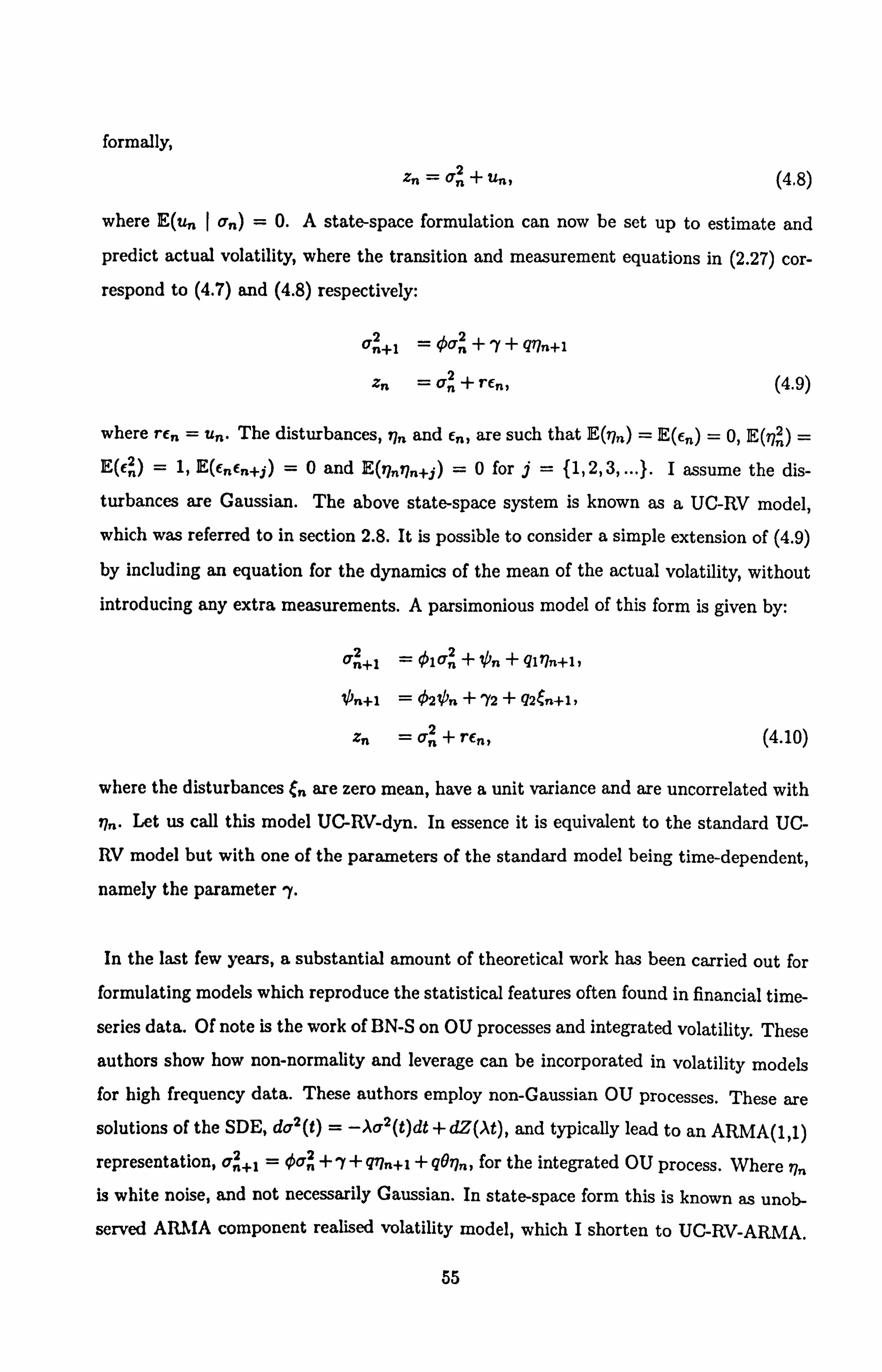
formally,

xn=Qn -Euni 2 (4.8)

where E(un I v,, ) = 0. A state-space formulation can now be set up to estimate and

predict actual volatility, where the transition and measurement equations in (2.27) cor-

respond to (4.7) and (4.8) respectively:

a2 2 1= qan +7+ g17n+l

zn =Qn+re , (4.9)

where re� = u,,. The disturbances, 17,, and e,,, are such that E(77n) = E(en) = 0, E(rin) = ]E(d) = 1, lE(enen+j) =0 and E(rjnr7�+j) =0 for j= {1,2,3,... }. I assume the dis-

turbances are Gaussian. The above state-space system is known as a UC-RV model,

which was referred to in section 2.8. It is possible to consider a simple extension of (4.9)

by including an equation for the dynamics of the mean of the actual volatility, without

introducing any extra measurements. A parsimonious model of this form is given by:

0, n+l = o1Qn + ipn + 91'Jn+1,

')n+l = 020n +72 + 92en+1,

Zn = cT + TEn, (4.10)

where the disturbances ý,, are zero mean, have a unit variance and are uncorrelated with

7 7.. Let us call this model UC-RV-dyn. In essence it is equivalent to the standard UC-

RV model but with one of the parameters of the standard model being time-dependent,

namely the parameter ry.

In the last few years, a substantial amount of theoretical work has been carried out for

formulating models which reproduce the statistical features often found in financial time-

series data. Of note is the work of BN-S on OU processes and integrated volatility. These

authors show how non-normality and leverage can be incorporated in volatility models for high frequency data. These authors employ non-Gaussian OU processes. These are

solutions of the SDE, da2(t) = -AQ2(t)dt+dZ(At), and typically lead to an ARMA(1,1)

representation, vn+1 = 0vn + If + 9r7n+1 + 4977n, for the integrated OU process. Where 77� is white noise, and not necessarily Gaussian. In state-space form this is known as unob-

served ARMA component realised volatility model, which I shorten to UC-RV-ARMA.

55

This model is implemented in this study. Instead of an ARMA(1,1) representation, the

UC-RV model (4.9) corresponds to an AR(1) representation for the actual volatility. One

of the differences between UC-RV and UC-RV-ARMA is that the former is computation-

ally more tractable.

BN-S show that it is possible to use a mixture (linear combination) of OU processes. In

this way o is composed of several OU processes or `components' which are superimposed.

These authors report positive results for this specification over using a single process. The

curse of dimensionality may hinder calibration for many components and in the literature

up to two or three components are used. Following BN-S I also consider superimposition

of autoregressive model components as referred to above. In detail,

an2 2 +1, j = q5jcn,

j + 7; + 4j? 7n+1, j, j= 1,2, ..., J J

Zn => orn2j + rcn, (4.11) j=1

where rE� = u� and the 77,, +I j are uncorrelated. As before the state equation innovations

are uncorrelated with the measurement noise. I call the above an UC-RV-J model. In

this way UC-RV-1 = UV-RV with 01 = 0, , y' = 7, qi =q and Qn, l = o, n" The authors

in Barndorff-Nielsen and Shephard (2002) show that ]E[(re,, )2] = r2 is a function of the

constant A, as well as the mean, variance and autocorrelation of the continuous time

OU process. These authors give the relation between these constants and the mean,

variance and covariance of the discrete-time model. However, practical implementation

of the dependence of r on these constants remains an issue. Instead I decide to estimate

the model without incorporating this dependence on these, i. e. I take r as a separate

parameter to be estimated. Koopman and Hol (2002) on the other hand restrict this

parameter to unity as they find that the model is not identified when this parameter is

implied as a function of A.

By following the model (4.1) I assume that there is no risk premium, or at least I do not

price market risk. This is also the approach taken in the seminal paper by Hull and White

(1987). Those econometricians that do price risk usually do so by jointly observing series

of option and spot prices and from differences in the dynamics of these two processes a

risk premium is inferred. Relevant references include the papers of Heston (1993), Bhar

56

et al. (2004) and Guo (1998). Compensation for investing in a risky asset is naturally an increasing function of the volatility of the asset. Clearly the simplest representation for

this compensation is direct proportionality, parameterised by a constant ß, say, so that if I were to price market risk (4.1) would become:

dS'(t) = (µ + QQ2(t))dt + Q(t)dW(t), (4.12)

where p is now the riskless growth rate. I do not price market risk in this context because

calculation of fl in particular in a fully specified UC-RV model is intractable. To see why

this is let us consider the conditional distribution for r,, = SZ(n0) - S1((n - 1)A) for a

time interval 0>0:

%'n I Qn ^' N(ILO /ýýný ýný (4.13)

Suppose w. l. o. g. that 0=1. Let us first consider the case where 3=0. Then the

daily returns have mean it and variance o n2, that can be estimated unbiasedly from M

intra-day demeaned returns as, M-I

Zn = {(n

-1)+('ýM1)S1{n-1)+-2(4.14) j=o

[Si

Jl

because p is known. However if ß#0 there is no way of obtaining an unbiased estimate

of on from RV. This is because the calculation of RV by subtracting ßo-, /M from the

intra-day returns is not possible as on and ß are the very quantities we are attempting to

estimate. The only alternative is to jointly estimate 0 and an in a fully specified model

of the form:

on+1 = oa +'i' + g77m+l

Tn =+ Pa; -i- Qnfn, l

Zn =Qn+r(n, 2 4.15)

where rn are daily returns and where z is calculated from (4.14). However there will be some biases involved because in (4.14) I assume ß=0 where as in (4.15) I assume

the model formulation (4.12) where Q ,-0. An attempt to work with this fully specified

model proved unsuccessful leading to numerical instabilities in the optimisation routine. Neglecting # in (4.15) led to successful estimation but no improvement in forecasting

performance nor fit of the data. Further details of this particular model will be left for

Chapter 6.

57

In the next section the calibration of the above models will be considered.

4.3 The calibration procedure for UC-RV models

For the calibration of the UC-RV models, the hidden state will be estimated using the

KF (Harvey, 1989, section 3.2) and the parameters by QMLE. The likelihood function

that is maximised has been given in (2.36) as:

TT

Llog(2T I B) _-E IogFn - vnFn-1. (4.16) n=1 n=1

From the output of the KF the maximum likelihood method will be used to estimate

the parameters. For brevity and simplicity of notation let us only consider the filtering

equations for the standard UC-RV model. The KF equations (2.31) for this model are:

Vn = zn - Q2 nln-1,

Fn = Pnin-1 + r2,

Kn = OPnln-1 Fn 1,

&n+1ln =0 non-1 + If + Kn'Un,

Pn+lln = 02Pnln-1 + q2 - K, 2 F,. (4.17)

Clearly estimation for the KF is carried out by one-step-ahead prediction. For multi-step

prediction the setup is similar to that of prediction with missing observations and we

simply step ahead without updating. Thus the estimate for the state for m steps ahead

takes the form:

M-1 0'n+m. ln -ýmo.

n+E'; O7l

j=0

(4.18)

From (2.33) the stationary mean and variance of the state is given by

lim 1E(o 10) = (1 - and lim Var(o 10) 02)-1q2. (4.19) n-. oo n-+oo

when E(QÖ) < oo and Var(öö) < oo. From (2.34) we can initialise the KF estimates for

the mean and variance of the initial state as these very equations:

äö = (1 - 0)-1-y, and Po = (1 - 02)-142" (4.20)

58

The assumption that the noise terms in (4.9) are Gaussian means that a standard Gaus-

sian filter, such as the KF can be applied to obtain the innovations and their conditional

variances. A Gaussian Filter being applied to a model which is not necessarily Gaussian

implies that the state estimates may be biased and thus the estimation will be subop-

timal. In QMLE these biases are ignored in the actual estimation. These are however

accounted for when calculating standard errors on the estimates (see Appendix A). The

KF can be extended to approximations which deal with models with non-linearity in

the state using suitable approximations. An Euler-Maruyama discretisation of the well known CIR or Feller model Cox et al. (1985b), gives,

an+l = oan +7+4 an r7n+1 1 (4.21

which provides a particularly simple extension and approximation. The only difference

for (4.17) is the last equation which is extended to P, i+i1 _ ¢2P 1 _1 +Q1 q2 - Kn Fn.

The vnln term has been substituted in for the unknown a. The implication of this ex-

tension is that P,, +11,, does not converge unlike the original model.

I will denote the above model as Gaussian UC-RV model with a Feller extension or

simply UC-RV-ext. This model along with the UC-RV-dyn model, the UC-RV-ARMA

model with one component3 and the UC-RV with one, two and three components are

the six models under consideration for the forecasting performance comparison. I denote

these models UC-RV-type models, to distinguish them from GARCH-type models, which

are discussed next.

4.4 GARCH model specification and calibration

It is of interest to consider GARCH models for two reasons. First, these are commonly

used in practice and serve as a useful benchmark. Second, as potential medium-term

forecasting models in their own right, I would like to verify which prediction method

works best for these models. The literature indicates that a parsimonious model such as GARCH(1,1), (3.9), is as good or better in terms of forecasting performance than stan- dard GARCH models with more than just one lag (see for example Hansen and Lunde

3The UC-RV-ARMA model with two components could not be identified due to instabilities in the

optimisation, leading to computational limitations. For this reason this model and the UC-RV-ARMA

model with three components were not implememted.

59

(2005a)). However, a term to allow for leverage is often introduced, such as in the GJR-

GARCH model, (3.10), as this is frequently demonstrated to bring some improvement.

GJR-GARCH is also known to perform better than some more complex models. Mar-

cucci (2005), for example, show that for a horizon of over one week this model performs

better than the more complicated Markov regime switching LARCH models. Another

popular forecasting model is the EWVMA model defined in section 3.1.2.

It is well known that daily returns are highly non-normal, and such was the case here

for the data used. Therefore maximising a likelihood function based on a Gaussian

distribution would lead to misspecification. To correct this Bollerslev (1987) suggested

employing the Student t-distribution for the calibration of the standard GARCH model.

The n-stage likelihood resulting from this distribution is:

r ý2 Z) )2 l-( z')

ý(E(n) I e, ý, º-ý) =r (2) (v ±2)U2(n)ý ý1 + (v

ý2)ý2(n)I (4.22)

where I'(. ) is the Gamma function and v>2 is the number of degrees of freedom. This

parameter is related to the degree of departure from a normal distribution which I take

simply as a parameter to be estimated. The e(n)'s are de-meaned daily returns calculated

from the daily opening and closing prices. I take the natural logarithm of the above to aid

computation of its maximum. To distinguish between the standard GARCH model with

a normal density calibration and the one using the above likelihood the latter is termed

GARCH-t. As the above likelihood is used in the GARCH-type models of this chapter,

I refer to these as GARCH-t, GJR-GARCH-t and EWMA-t. I estimate these models

by maximising the likelihood of the de-meaned daily returns. Obviously, it is expected

that intra-day data used in UC-RV type models represents additional, non-redundant

information as compared to the daily data used in GARCH-type models. One therefore

expects that UC-RV-type models will outperform GARCH-type models when it comes

to prediction. However, it is still worth validating this expectation in practice. Further,

GARCH-type models with daily data serve as useful and industry-standard benchmarks

against which to compare other models for volatility prediction.

60

4.5 Medium-term horizon forecasting: implementation and

comparison study

Having set up the models to be employed and their calibration procedures, the objec-

tive of this work is to look at choosing a suitable procedure for estimating ten-day-ahead

volatility. To be consistent with the procedures of the Basel Capital Accord' the constant

volatility methods considered here will be limited to scaling sixty and one-day volatility

estimates. For the dynamic volatility models employed here there are several ways that

volatility can be predicted. For the UC-RV-type models in particular, one can rely on

multi-step prediction, lengthen the sampling interval or scale a short horizon prediction.

For the multi-step method, ten-step-ahead forecasts will be produced for the shorter

sampling interval of one day. The cumulative predicted volatility from the one-step up

to ten-step predictions will be taken as the volatility estimate over the ten-day horizon.

For the second method the sampling interval is lengthened to ten days. In this way the

same forecasting horizon of ten days can be considered for the one-step-ahead forecasts

for this sampling interval as for the multi-step forecasts with a sampling interval of a day.

The last method will assume a one-step-ahead forecast for the shorter sampling interval

of one day and scale this by ten. Although a number of authors advise against scaling

procedures (Christoffersen et al. (1998), Blake et al. (2000)) they are a standard practice

in the finance industry and may not be a bad approximation for horizons of just ten

days. Moreover, I take the practical approach of evaluating methods in terms of their

forecasting performance.

I perform a similar comparison of two different methods of volatility prediction for

LARCH-type models. In contrast to the UC-RV-type models, there are two main ways

that the volatility can be predicted using GARCH-type models: (a) multi-step prediction

using one-day forecasts, and (b) one-step-ahead for one day and scaling this by a factor

of ten. For (a) there is a simple expression for the m-step GARCH(1,1) formulation:

M-1 m

a2(n + m) = ßmv2(n) +7E, 0'+ a+m- i)2. (4.23) i=O i=l

The expression (4.23) can readily be modified for GJR-GARCH and EWMA. The calibra-

tion of these models indicated that GJR-GARCH-t fitted the data better than GARCH-t, "Although the procedures of which do not cover all companies, they are currently restricted to banks.

61

which agrees with the literature. For the scaling method (b) I followed the UC-RV-type

scaling procedure by factoring a one-day forecast by ten. Apart from (a) and (b) an-

other approach that could be considered is that of temporal aggregation. As has been

pointed out, Drost and Nijman (1993) and Drost and Werker (1996) showed how certain

GARCH models at one frequency could be inferred from models at another frequency. In

the present context this would mean we could estimate the model at a daily frequency,

say, and infer a model for ten-days. However temporal aggregation is not appropriate

here as the GARCH formulation (3.9) I assume is semi-strong GARCH. Drost and Nij-

man (1993) showed that semi-strong GARCH aggregates to weak GARCH which means

that we would lose the assumed GARCH structure for a ten-day model. As well as the

above papers I refer interested readers to (Meddahi and Renault, 2000, p. 1-2) for more

thorough explanations.

Forecasting performance is evaluated by an appropriate loss function. Among all possible

choices of commonly employed loss functions in the literature, only two are known to be

robust to the presence of noise in the chosen volatility proxy. Patton (2006) has shown

that these are the MSE loss function and the QLIKE loss function. It is the former

that I focus on as it has a more direct interpretation than the latter and is much more

commonly employed. It is simply defined as:

Lf = E(Q2 - 2)2. (4.24)

where 2= zn + z,, +l + ... + zn+9 and where Q2 is defined differently for each prediction

method. For multi-step prediction, Q2 = Qnin_1 + 0'n+1ln-1 + ýn+21n-1 + '+' 0'n+9In-1;

for the scaling method v2 = 1OQnýn_1 and for the one-step ten-day interval a2 = výIM_1,

where m is the index for a ten-day interval. Clearly the MSE loss function is not

heteroskedasticity-adjusted (i. e. innovations of a large magnitude are not given less

weight), which is consistent with the application of VaR estimation for which it is not

desirable that innovations of a large magnitude be scaled down.

I now proceed to the actual implementation of the models.

62

4.5.1 The data

A relevant data sets of two very liquid assets was used as input to the UC-RV-type and

GARCH-type models. PriceData provided 5 minute intra-day data for IBM and Cit-

igroup. Stocks from these companies trade mainly on the New York Stock Exchange

which is open from 9: 30 to 16 : 00, during business days. I took the opening price of

each 5-minute bar. The data provided consisted of the price level from August 1997 to

March 2005 giving over 148000 observations. From this I took the first 147420 returns

corresponding to N= 1890 data-days given that there were 78 bars per day. An issue

that often arises in using financial data is that of price discreteness, i. e. the price of the

asset frequently remains at a given level for relatively long periods of time. Given that

the stocks I employ are very liquid we expect that there will be sufficient trading for price

changes to occur within the five minute intervals and thus not to suffer from noticeable

price discreteness.

There is increased trading activity/large price changes in the morning, when macroeco-

nomic news arrives6, and late afternoon, but since I consider daily volatility estimates7

this intraday seasonality will not be of any direct relevances. The issue of overnight

variation is, on the other hand, an important issue and will be discussed in the next sec-

tion. Clearly markets are closed at weekends and holidays which implies a large amount

of missing data. There are different ways of dealing with missing `observations'. In the

case of the KF the recursions can be run with some modifications when observations are

missing. Non-trading days in the literature are however generally ignored, cf. Andersen

et al. (1999b). A possible reason for this is that weekends and holidays together make

up a substantial amount of the total data, too much to be treated as missing. It seemed

"Denoted data set 1. ®Due to the importance of the US on the global economy, markets outside of the US will see the

effects of macroeconomic news release, but clearly mostly at other times of the day (cf. Areal and Taylor

(2002)). 'For a shorter estimation window we would have to take this into consideration. On the other hand for

a longer RV estimation window such as a week or ten days we would not need to worry about intra-weekly

variation, i. e. the fact that on Mondays and Fridays volatility generally is larger than other days of the

week. This issue is discussed in the following section (4.5.2). "Assuming an additive structure of the diurnal effects as explained in (Barndorf Nielsen and Shephard,

2002, section 6).

63

better to collapse the series down than to artificially attempt to model it. Therefore, as

is the general practice among econometricians, days that contained no data whatsoever

were ignored. The market closes early on the eve of certain holidays and there were also

some missing data unrelated to any market closure, probably due to a breakdown in the

data feed. To deal with this the data were preprocessed by stochastically interpolating

any missing values in the data series within a one-day period. The standard deviation

value used in the interpolation was an average of standard deviation values from a group

of sub-intervals proceeding the missing price range. The reason for using an average of

sub-interval values was to lessen the dependence of the standard deviation on the drift,

the impact of which was seen to be otherwise quite significant. It should be noted that

preprocessing the data had little impact on the total variation of the data, i. e. the vari-

ance of the raw data with missing prices replaced by zero and the variance of the data

after the intervention were very similar. The fact that after carrying out the preprocess-

ing every trading day contained a full set of stock prices meant that I could proceed to

estimating a model for sampling intervals of one day (or multiples of one day). The series

was multiplied through by 100 so that the returns are expressed as a percentage. The

daily returns, R,,, are defined as 100[S' (n) - S1(n - 1)] where St (n) is the log-price level

for the last bar of day n.

The stock price path was sampled every five minutes corresponding to M= 78 in (3.15)

for A=1. There has been a substantial amount of work on the choice of sampling

frequency in the already cited papers of Bandi and Russell (2006), Ait-Sahalia et al.

(2005) and Oomen (2002). The first authors show that the optimal frequency for the

stocks I consider here is around 2.6 minutes. However this can be seen as an approximate

guideline as other research is more conservative in regards to this value. Moreover the

research of Bandi and Russell (2006) is based on prices from quotes rather than the actual

transaction prices used here. Five minutes is the highest frequency available to us and is

a commonly used frequency in the literature.

4.5.2 Realised volatility estimation

Calculating RV purely from the equation (3.15) ignores the fact that overnight returns will

be generally substantially larger than intra-day ones. Using one return value to represent

64

the overnight volatility will have a distorting effect on the daily volatility estimate. One

way around this is to calculate purely the volatility during trading hours. Martens

(2002) suggests scaling this trading-hours estimate to account for overnight volatility.

The scaling factor he suggests is 1+c= (am + Q, )/cam where 0,2 and a, 2, are the in-

sample open-to-close and close-to-open variances respectively. In this way the overnight

volatility is averaged out over the whole sample leading to a smoother volatility series

than would otherwise be the case. In detail the scaled daily volatility estimate

Zn =(l+c)ýE LIS'{(n-1)0+A(M

1)Sl

l(n-1)0+

Lj 2 (4.25)

ý-1 l JJ

is the one employed here for an interval of one day9. As in Koopman and Hol (2002),

for intervals of longer than one day I simply use the cumulative sum of days in the RV

series calculated from (4.25). The value for (1 +c) I obtain is 1.357 for IBM and 1.307 for

Citigroup, which is somewhat higher than the value of 1.205 observed by Martens (2002).

There are other methods of dealing with overnight returns that have been proposed and

implemented. Areal and Taylor (2002) propose using unequal weights in (3.15), which,

using an "optimum" weighting scheme based on minimising the variance of the RV es-

timate, leads to a relatively small weight for the overnight return. Hansen and Lunde

(2005b) carry out a similar approach in considerable depth as well as also suggesting

a scaling procedure similar to that in Martens (2002). In this thesis I use the scaling

method of Martens (2002). It is also the method that is implemented in a paper of special

relevance here of Koopman et al. (2005) in which the forecasting performance of UC-RV

models is also consideredio

The issue of the larger variance on Mondays due to over-weekend returns being poten-

tially larger than overnight ones is not relevant here given the way I treat overnight/over-

weekend returns. On the other hand there is the issue of intra-weekly seasonality resulting

from from increasing trading at the beginning and end of the week. This implies that

'In calculating the open-to-close and close-to-open variances, outliers in the close-to-open series that

had an effect above and beyond the outliers in the open-to-close series were removed. Making a dis-

tinction between weekday and weekend overnight returns was considered but the implementation showed

that there was little difference between over-weekend close-to-open variance and weekday close-to-open

variance. '°More will be said on this in chapter 6.

65

there is a mismatch between a one-day estimation window/horizon and a ten-day esti-

mation window/horizon. I give an example to make this clearer. If we use a volatility

estimate/forecast for a Friday, say, to forecast ten days ahead the forecast of the volatil-

ity for this horizon will probably be larger than the forecast when using a Thursday,

say. This mismatch comes as a direct result of the fact that for an estimation window of

ten days, such as the one employed here, any intra-week patterns are not of relevance,

as has been mentioned. This fact clearly also applies to a forecast horizon of ten days.

Essentially, the longer the forecast horizon/estimation window the less we need to worry

about patterns in the volatility"

Clearly I have ignored µ/14T in the calculation of (3.15), and hence also in (4.25), but

the contribution of this constant is negligible. I use (4.25) for the RV measurements for

the models that were estimated.

Descriptive statistics for data set 1 appear in table 4.1. From this table we can see

that the daily log-return and squared log-return series are far from normal which is in

keeping with the non-Gaussian property of daily series in the literature. Hence a fat-tailed

distribution for the GARCH-type models as given earlier is appropriate. I should point

out that the data set used and preprocessing procedures employed here are suited for

VaR estimation for two reasons. Firstly, no outliers in the RV series have been removed

and thus taking into consideration extreme events. Secondly, I use a large window of data

(over seven and a half years) that includes market crashes and company acquisitions that

induce large shifts in the price level; which explains the large magnitude of some of the

values in the above table. Although the RV series are far from normal they are close to

lognormal. Introducing the log-transformed RV series as the observation process in (4.9)

produced spurious results however. This is not surprising as the literature indicates that

log RV displays long memory that would rely on other techniques12

"To put some caveats on this conclusion there is also evidence of intra-monthly and even intra-yearly

effects corresponding to month and yearly seasonals, respectively. This means that there may still be

some loss of statistical accuracy for longer horizons and estimation windows with these seasonals ignored. 12Long memory, as has been pointed out, is often modelled using an auto regressive fractionally inte-

grated moving average (ARFIMA) model or in the GARCH framework, the FIGARCH model of Bollerslev

et al. (1996).

66

Table 4.1: Descriptive statistics for the daily log-return, the squared daily log-return and

the RV (for M= 78,0 = 1) series of data set 1.

IBM stock Citigroup stock

Statistic Rn Rn Zn Rn Rn Zn

Mean 0.03 5.16 4.51 0.03 5.61 6.40

Variance 5.16 303.03 28.00 5.61 319.16 84.77

Skewness -0.27 14.23 5.54 0.36 17.74 6.79

Excess Kurtosis 9.41 295.51 53.87 6.56 472.28 69.38

Maximum 14.54 456.65 77.52 23.38 546.44 137.30

Minimum -21.37 0 0.18 -16.50 0 0.28

Q(12) 18.88 49.30 2822.32 12.34 161.32 2811.31

Q(l) is the Box-Ljung portmanteau statistic based on I squared autocorrelations. The hypothesis

of no autocorrelation cannot be rejected for the daily log-returns for both stocks at any standard

significance level given the low values of Q(12). To reject this hypothesis we would need Q(12)

values of 21.03 for 95%-certainty and 26.22 for 99%-certainty levels.

4.5.3 Parameter estimates and standard errors of UC-RV and GARCH-

type models

The optimisation of (4.16) was carried out using Matlab's fmincon algorithm for con-

strained nonlinear optimisation. This is an algorithm tuned to finding the optimum

parameter vector of a non-linear function of several variables with constraints. It uses

a sequential quadratic programming method. In this method, the function solves a

quadratic programming problem at each iteration. An estimate of the Hessian of the

Lagrangian is updated using the Broyden-Fletcher-Goldfarb-Shanno (BFGS) formula,

Broyden (1970), Fletcher (1970), Goldfarb (1970) and Shanno (1970). In the models in

question there are natural constraints on some of the variables such as 01 < 1,02 < 113

and 0< ql, q2, r< oo. Starting off with these it became apparent that local optima were

being found. Having some idea of the magnitude of the parameters some of the bounds

were then tightened. After carrying this out better (and probably global) optima were 13This constraint assures some degree of stationarity and is a consequence of the assumed underlying

dynamics.

67

arrived at.

Of the six UC-RV-type models mentioned, only four were actually used in the compar-

ison study. UC-RV-ARMA for IBM for A= 10 led to an insignificant value for £, the

very parameter that causes this model to differ from UC-RV. Moreover its forecasting

performance was significantly worse than UC-RV. On the other hand the optimisation of

UC-RV-3 model led to unacceptably large standard errors on the parameters. For these

reasons the calibration results and forecasting performance of the UC-RV-ARMA and

UC-RV-3 models are not reported. The four that remain for exposition therefore are

UC-RV, UC-RV-2, UC-RV-dyn and UC-RV-ext. All of these were previously defined in

sections 4.2 and 4.3.

A Bayesian approach to parameter estimation would be to find the whole distribution of

the parameter estimates. This is carried out using prior information on the parameters'

distributions together with a likelihood function. Here the classical approach is taken

where only the first two moments of the parameter estimates' distribution are consid-

ered. The parameter estimates obtained from the optimisation corresponds to the first

moment. The `standard errors' correspond to the second moment, i. e. the square root of

the diagonal entries of the parameter covariance matrix. This matrix was estimated tak-

ing into account the non-normality of disturbances and as such I will refer to the errors

being QMLE standard errors. I follow the information matrix approach as detailed in

(Hamilton, 1994, section 5.8). For QMLE the estimation of the covariance matrix for this

approach involves both the outer product estimate or the second derivative estimate of

the information matrix. The estimates for 011 027 'yl, Y2, ql, q2 and r for the UC-RV-type

models together with the standard errors14 in brackets are given in the tables 4.2 and 4.3.

The standard errors in tables 4.2 and 4.3 have been normalised w. r. t. their nominal

values, i. e. I divide through by the actual parameter estimates. The zero values for the

parameter r come as a consequence of lack of convergence in Pn, In_1 which is reflected

in the estimation of F� and hence in r as well. The normalised standard errors on the 14 The approximations involved in the UC-RV-ext model limit to some extent the relevance of standard

errors and as such they are not displayed. Parameter estimates that take values less than 5* 10-3 appear

as 0.00 In the table and are insignificant relative to other parameter values in all cases

68

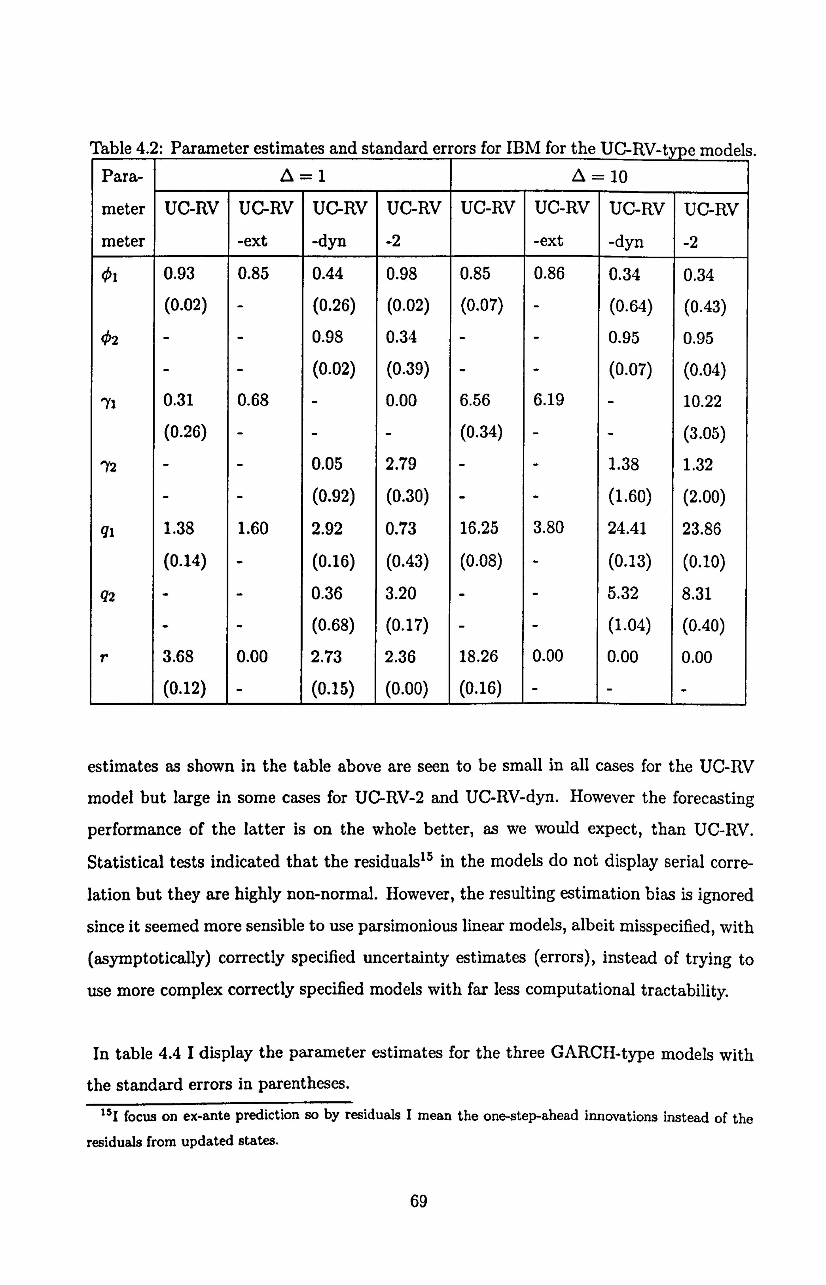
Table 4.2: Parameter estimates and standard errors for IBM for the UC-RV-type models. Para- L=1 0=10

meter UC-RV UC-RV UC-RV UC-RV UC-RV UC-RV UC-RV UC-RV

meter -ext -dyn -2 -ext -dyn -2 O1 0.93 0.85 0.44 0.98 0.85 0.86 0.34 0.34

(0.02) - (0.26) (0.02) (0.07) - (0.64) (0.43)

02 - - 0.98 0.34 - - 0.95 0.95

- - (0.02) (0.39) - - (0.07) (0.04)

yl 0.31 0.68 - 0.00 6.56 6.19 - 10.22

(0.26) - - - (0.34) - - (3.05)

IM - - 0.05 2.79 - - 1.38 1.32

- - (0.92) (0.30) - - (1.60) (2.00)

ql 1.38 1.60 2.92 0.73 16.25 3.80 24.41 23.86

(0.14) - (0.16) (0.43) (0.08) - (0.13) (0.10)

Q2 - - 0.36 3.20 - - 5.32 8.31

- - (0.68) (0.17) - - (1.04) (0.40)

r 3.68 0.00 2.73 2.36 18.26 0.00 0.00 0.00

(0.12) - (0.15) (0.00) (0.16) - - -

estimates as shown in the table above are seen to be small in all cases for the UC-RV

model but large in some cases for UC-RV-2 and UC-RV-dyn. However the forecasting

performance of the latter is on the whole better, as we would expect, than UC-RV.

Statistical tests indicated that the residuals15 in the models do not display serial corre-

lation but they are highly non-normal. However, the resulting estimation bias is ignored

since it seemed more sensible to use parsimonious linear models, albeit misspecified, with

(asymptotically) correctly specified uncertainty estimates (errors), instead of trying to

use more complex correctly specified models with far less computational tractability.

In table 4.4 I display the parameter estimates for the three GARCH-type models with

the standard errors in parentheses. 151 focus on ex-ante prediction so by residuals I mean the one-step-ahead innovations instead of the

residuals from updated states.

69

Table 4.3: Parameter estimates and standard errors for the UC-RU type models for the

Citigroup stock. Para- A=1 0=10

meter UC-RV UC-RV UC-RV UC-RV UC-RV UC-RV UC-RV UC-RV

meter -ext -dyn -2 -ext -dyn -2 O1 0.89 0.88 0.89 0.98 0.79 0.88 0.38 0.98

(0.04) - (0.10) (0.01) (0.12) - (4.80) (0.05)

102 - - 0.46 0.67 - - 0.76 0.76

- - (11.36) (0.23) - - (0.49) (0.47)

ryl 0.71 0.76 - 0.11 13.37 7.48 - 0.00

(0.30) - - (2.45) (0.38) - - -

72 - - 0.38 0.33 - - 9.26 14.38

- - (9.01) (12.81) - - (1.58) (2.12)

ql 3.32 2.18 3.31 1.07 33.32 5.61 0.35 4.75

(0.23) - (0.72) (0.42) (0.12) - (56.33) (0.57)

q2 - - 0.00 4.14 - - 23.31 33.34

- - - (0.26) - - (1.99) (0.80)

r 5.70 5.79 5.70 5.13 34.40 0.00 38.57 33.82

(0.12) - (0.18) (0.00) (0.24) - (0.46) (0.68)

Table 4.4: Parameter estimates and standard errors for the GARCH-type models for the

IBM and Citigroup stocks.

IBM stock Citigroup stock

GARCH-t GJR-GARCH-t EWMA-t GARCH-t GJR-GARCH-t EWMA-t

ry 0.00 - 0.00- - 0.02 (0.48) 0.01(0.60) - Q 0.97 (0.00) 0.97 (0.00) 0.98 (0.00) 0.93 (0.01) 0.95 (0.01) 0.95 (0.01)

a 0.03 (0.16) 0.01 (0.77) 0.02 (0.19) 0.07 (0.14) 0.01 (0.52) 0.05 (0.15)

A - 0.04 (0.25) - - 0.08 (0.18) -

v 4.54 (0.04) 4.75 (0.04) 4.56(0.04) 6.07(0.04) 6.33 (0.04) 6.57(0.04)

70

The standard errors proceed from standard maximum likelihood estimation calculations.

For standard maximum likelihood using the information matrix approach, the covariance

matrix is based on either the outer product estimate or the second derivative estimate

of the information matrix's. This differs from the QMLE procedure employed for the

UC-RV-type models, where the covariance matrix is based on a weighted average of the

two information matrix estimates. For misspecified models, such as UC-RV-type models,

QMLE should be employed. In contrast, if a model is assumed to be correctly specified,

such as GARCH-t, standard maximum likelihood can be employed. The standard errors

have been normalised in the same way as explained earlier and as such correspond to

percentage errors. Although a few of the standard errors are large the models perform

significantly better in terms of forecasting performance than their counterparts calibrated

using a Gaussian distribution, as would be expected. Numerical results for Gaussian

GARCH-type models are omitted for brevity.

4.5.4 Comparison study

In this section I will compare UC-RV-type models against constant volatility and GARCH-

type model estimates in terms of forecasting performance. Although it may seem trivial

to make comparisons with methods based on constant volatility, the financial practice fre-

quently employs the latter. Moreover the estimation results show that constant volatility

methods even outperforms GARCH-type models for the IBM stock17. In tables 4.5,4.6,

4.7 and 4.8 the forecasting performance for the three groups of models are displayed. To

aid the presentation of results I give a summary of the terms and methods employed:

" `One-day': RV calculated over the previous day to the first day of the forecast

horizon.

9 `Sixty-day': RV calculated as the average of the sixty one-day RV's previous to the

first day of the forecast horizon 18.

9 `Ten-step, one-day': a sampling interval of one day with ten-step-ahead prediction

using (4.18).

161 base the covariance matrix of the parameter estimates on the outer product estimate of the infor-

mation matrix. "To put some caveats on these conclusions GARCH-type models do not use RV. '8because of overnight returns I prefer this approach to that of simply calculating RV over a sixty-day

period.

71

. `One-step, ten-day': a sampling interval of ten days with one-step-ahead prediction.

" `One-day scaled': for a sampling interval of one day, one-day-ahead prediction

scaled by ten.

Table 4.5: Loss function values for the three volatility prediction methods for the UC-

RV-type models for the IBM stock Ten-step, one-day One-step, ten-day One day scaled

UC-RV 702.56 694.55 724.51

UC-RV-ext 694.58 757.15 623.30

UC-RV-dyn 648.74 674.47 593.32

UC-RV-2 653.39 674.43 593.28

The performance is based on the MSE loss function Lf (4.24) over the whole sample.

For the UC-RV-type models let us recall the three prediction methods: (a) ten-steps-

ahead using (4.18) for a one-day sampling interval against (b) only one-step-ahead for

a longer sampling interval of ten days and (c) one-step-ahead for the shorter sampling

interval and scaling this by a factor of ten. For the GARCH-type models let us recall

the two prediction methods: (a) ten-steps-ahead using (4.23) and (b) one-step-ahead and

scaling this by a factor of ten.

Table 4.6: Loss function values for the three volatility prediction methods for the UC-

RV-type models for the Citigroup stock Ten-step, one-day One-step, ten-day One day scaled

UC-RV 2431.76 2627.20 2101.75

UC-RV-ext 2266.43 3089.21 2197.47

UC-RV-dyn 2428.72 2627.11 2102.08

UC-RV-2 2298.76 2621.29 2083.96

Let us analyse the results table by table. First of all starting with table 4.5 we see

that for three out of the four models the scaling method performs the best followed by

multi-step forecasting followed by the "One-step, ten-day" interval method. Moreover

72

Table 4.7: Loss function values for the two constant volatility methods for the IBM and

Citigroup stocks. IBM stock Citigroup stock

One day Sixty day One day Sixty day

707.47 828.39 2385.40 3477.58

Table 4.8: Loss function values for the two volatility prediction methods for the GARCH-

type models for the IBM and Citigroup stocks. IBM, one-day scaled IBM, multi-step prediction

GARCH-t GJR-GARCH-t EWMA-t GARCH-t GJR-GARCH-t EWMA-t

1142.25 1323.22 1168.16 971.33 1066.52 996.00

Citigroup, one-day scaled Citigroup, multi-step prediction

GARCH-t GJR-GARCH-t EWMA-t GARCH-t GJR-GARCH-t EWMA-t

3402.81 2723.13 3401.52 2564.52 1994.74 2728.56

the scaling method is statistically significantly better19 than the multi-step method in

these three cases. We also note that the two state models, UC-RV-2 and UC-RV-dyn,

perform consistently better than the one-state models20. For the Citigroup stock the

pattern of results is similar. Considering table 4.6 we see that the scaling method is

consistently better than the multi-step method and the difference is statistically signif-

icant in all four cases. As before the "One-step, ten-day" interval method lags behind.

The two-state methods in general perform better than the one-state models although far

from consistently. We immediately notice the much larger magnitude in the loss function

values as compared to those of the IBM stock, which come as a direct consequence of the

comparatively large magnitude of the moments in the Citigroup RV series as reported

in table 4.1. In summary for both stocks we have that for the UC-RV-type models the

scaling method is statistically significantly better than the "One-step, ten-day" interval

method and than the multi-step method in seven out of eight cases. This point, and

the near complete consistency of these results lead us to conclude that for the data set "Using the likelihood ratio test for MSE developed by Holst and Thyregod (1999) for a critical value

of 0.01. "In detail model comparison in terms of statistical significance will be left for Chapter 6.

73

and methods employed scaling is indeed the best method for volatility prediction using

UC-RV-type models.

Table 4.7 simply shows that for both stocks the constant volatility method for one day

outperforms that calculated over sixty days. I should point out that the difference is

statistically significant. In table 4.8 I display the results for the GARCH-type models

using a t-distribution21. We immediately notice that in contrast to the situation in the

UC-RV-type models, for the GARCH-type models, multi-step forecasting performs con-

sistently better (and the difference is statistically significantly) than the scaling method

for both stocks. When it comes to cross comparisons of the GARCH-type models there

are discrepancies in performance patterns between the two stocks. For the Citigroup

stock the GJR-GARCH-t model performs the best for both methods whereas for the

IBM stock it performs the worse, the EWMA-t and GARCH-t performing closely.

Finally I will carry out cross comparisons of all the tables. For the UC-RV-type model

and selecting the best method the performance is better than the best method for con-

stant volatility in seven out of eight cases. Moreover the difference in all these seven cases

is statistically significant for a critical value of 0.01 and it is not statistically significant

in the case where one of UC-RV-type models does not perform better than the constant

volatility. As a whole we can observe that the UC-RV-type models perform statistically

significantly better overall than the GARCH-type models although there is a noticeable

exception: the multi-step method for GJR-LARCH for the Citigroup stock performs

statistically significantly better than all other models and prediction methods for this

stock.

4.6 Conclusion

The contributions of this chapter are three-fold. Firstly, I have illustrated the estimation

and calibration of UC-RV-type models using high frequency asset price data and GARCH-

"The results for a normal distribution are omitted for brevity but I should point out that for the

t-distribution approach the performance was consistently better than the Gaussian case as we would

expect.

74

type models with a t-distribution and daily data. Secondly, the UC-RV-type models

have been compared with constant volatility and GARCH-type models for ten-day-ahead

volatility estimation. Thirdly, I have considered different prediction methods using each

model in terms of medium-term horizon forecasting performance. The conclusions from

the numerical study summarised in the previous section provide a valuable insight into

the choice of models and the choice of the prediction method within each model. At

the very least, these experiments suggest that simple filtering models such as the ones

presented here have a role to play in volatility forecasting.

75

Chapter 5

Medium-term horizon forecasting

for UC-RV models with implied

volatility

I now seek to consider state-space estimation of volatility using information coming from

the derivatives market. In detail, I estimate the market's expectation of future volatil-

ity as implied from short-term optionsl on an index as well as RV from high frequency

returns. Implied volatility will be used to forecast future volatility. The motivation for

this approach has been referred to in section 3.5. Although there are SV models that are

based on derivative price information alone, here we will follow the strand of research

that combines both stock return and option price information in estimating and forecast-

ing volatility. As is common practice in a substantial part of this line of research, it is

assumed that there is no risk premium, i. e. the objective and risk-neutral measures for

simplicity are assumed to coincide.

In recent years there has been increasing interest in using IV in forecasting volatility.

Although initial work in this direction followed soon after the introduction of the Black-

Scholes option pricing model, more recent contributions are of more relevance to this

thesis. From a series of seminal papers in the 1990's (Day and Lewis (1992), Lamoureux

'By short-term options I mean options with maturities of a couple of weeks or months. I am not

referring to the horizon of a forecast based on high frequency data because in this case short-term would

mean typically one day and medium-term a couple of weeks.

76

and Lastrapes (1993), Canina and Figlewski (1993), Jorion (1995), Taylor and Xu (1997)

and Christensen and Prabhala (1998)), no consensus was arrived at as to whether or

not IV subsumes the information already found in past returns in forecasting volatility.

However several of of the above contributions along with subsequent research do point to

incremental information found in IV. Moreover, several authors indicate possible reasons

why there was much inconsistency in the conclusions of the already cited papers. This

is mainly related to the statistical artifacts in the forecasting procedures which will be

pointed out in this contribution when the methodology is presented. The volume of trade

may also be a significant influence (see Mayhew and Stivers (2003)).

Like RV, IV is also subject to distorting biases by the way of measurement noise. Jorion

(1995) and Christensen and Prabhala (1998) among many others point out some of the

factors that contribute to the presence of measurement noise in IV. Most research ig-

nores this noise and simply introduces IV as an (extra) regressor in a forecasting model;

cf. Mayhew and Stivers (2003) and Canina and Figlewski (1993). Mayhew and Stivers

(2003) in particular show that introducing IV as a regressor outperforms high-frequency

GARCH. Other researchers take the noise into account in the models employed. For

example Christensen and Prabhala (1998), hereafter CP, do this using an Instrumental

Variables approach. This allows for corrective estimation of an error-in-variables regres-

sion resulting from the measurement noise biases. In detail these authors regress future

RV on past IV and RV. These authors show that IV outperforms RV in forecasting fu-

ture volatility for a monthly horizon. Their work extends previous research on forecasting

volatility of an index.

Here I wish to consider forecasting the volatility for individual stocks for a shorter, ten-

day horizon. The IV estimate that will be employed proceeds from the price of the index

of which the stocks in this study are components of. The motivation for this approach is

both practical and intuitive as detailed in section 5.2.

As far as I know, there has been no work carried out using UC-RV models together

with IV measurements, which warrants my study. I will consider filtering to deal with

the measurement error. In this setting I will use a two-dimensional state-space model

77

in keeping with the focus on linear estimation. Calibrating a UC-RV model using IV

measurements is to my knowledge, a completely new approach. In keeping with chapter

4, I shall consider ten-day ahead forecasting. This time-horizon, as opposed to a shorter

horizon of one day, say, is also chosen for a practical reason. The time to expiration of

options on stocks that are useful for volatility inference is medium to long-term, typically

a couple of weeks to a couple of months or even longer. We can think of the volatility

estimates implied from options as the average volatility over this time to expiration. For

this reason, a ten-day-horizon forecast is more consistent with the option IV information.

A longer time-horizon, such as a month, is seen to be beyond the scope of the focus of

this thesis. Furthermore for one-month-ahead volatility forecasts that are partly based

on a time series of high frequency returns, the mismatch between the forecast horizon

and the sampling frequency of these very returns is more apparent.

Before proceeding to the model setup the details pertaining to the estimation of the IV

series will be presented.

5.1 Implied volatility estimation

Although more complicated option pricing models can be employed, standard valuation

for vanilla options is carried out using the Black-Scholes formula for European options

and binomial tree methods for American options. A fundamental characteristic of these

models is that the volatility implied by option prices can be recovered if the strike price,

time to maturity, underlying price and interest rate are known. Although these methods

assume constant volatility, this can be viewed as the average volatility over the lifetime of

the option. A `continuous daily series' of IV's can be constructed by backing out volatility

from daily quoted or traded options for maturity dates usually between two weeks and

a few months depending on the series. These IV's will be subject to measurement error

due to, for example, bid-ask spreads, using approximations for inputs like for e. g. a proxy

interest rate, ignoring dividends, discrepancies in stock and option market closing times

and clerical measurement error. This measurement error will lead to biased estimates of

IV. Filtering the measurement noise can be carried out simultaneously with filtering the

noise implicit in RV employing a relatively parsimonious model structure.

78

The model employed finds IV via the Black-Scholes framework even though researchers

have shown that stochastic volatility and/or jump models better explain the properties

of option prices. There are three points to consider that warrant the constant volatility-

based approach. The first is practical. As pointed out in section 3.5, dynamic volatility

models can be calibrated from option prices using a direct approach; this involves identi-

fying model parameters that best match observed option prices. However, unlike GARCH

models, implied parameters do not completely specify the UC-RV models used in this

study. For complete specification we would need to augment the estimation procedure to

include the latent state. The curse of dimensionality hinders implementation as compu-

tational considerations are an issue: this approach would call for a Bayesian setup using

the computationally intensive MCMC. 2 Moreover the aforementioned direct approach

would involve modelling the spot price dynamics, something that is again beyond the

scope of the present work. Another reason why I stick to constant volatility models is

that among practitioners these are still overall very popular so it seems sensible to imply

volatility from the actual models used in valuation. Thirdly, Chesney and Scott (1989)

has shown that the disparity between constant and SV option valuation is quite small

for near-the-money options3 such as the ones employed in this study. Next the IV series

construction will be described.

Datastream provided a daily series of IV's, which I denote by IVdj, for the Dow Jones

Industrial Average (DJX) as underlying from 25/09/01 to 10/03/05. Options on this

index are European style and the IV is derived from the B-S model. Dividends and an

interest rate proxy are included in the model. The IVdj series uses month options in its

derivation. These expire on the Saturday after the third Friday of the month. DJX fol-

lows a March cycle. The March cycle consists of the months of March, June, September

and December. If the expiration date for the current month has not been reached, stock

options trade with expiration dates in the current month, the following month and the

next two months in the cycle. To limit the use of options that are very near to expiry

or very far to expiry, IVdj uses options that expire in the following month. Since IVdj

jumps to the `next available month options' when it reaches the expiry month, the time

2This procedure has been carried out in this context by, for example, Eraker (2004) and Poison and Stroud (2002).

3provided the time-to-maturity coincides between the constant and stochastic volatility models.

79

to expiration of the options is always at least two weeks and two days from the date

of the series and up to one month three weeks and a day. In trading days this corre-

sponds to between eleven and thirty-seven days. Thus on average the time to expiration

is of about twenty-four trading days, just over a month. Although the ideal would be

a constant time to expiration, to produce a daily series, a variable time to expiration

is needed'. Moreover it is not uncommon in the literature for it to be variable (as for

example in Taylor and Xu (1997)). In keeping with the focus of this thesis I consider

a ten-day forecast horizon. Clearly there is a discrepancy between the forecast horizon

and the time-horizon of the options. This horizon mismatch is common in the literature.

Blair et al. (2001), for example, use IV with a month to expiry for as short as a one-day

forecast horizon. Moreover it is plausible that in a option expiring in a month, say, most

of the expectancy of what the volatility is likely to be that is used to price the option will

pertain to the first couple of weeks or even first couple of days. This is a natural conse-

quence of the fact that it is hard to make accurate long-term predictions. If the horizon

is relatively long-term it may be better to simply extrapolate a shorter-term prediction.

In this case using the IV measurement from a month option to forecast over a two-week

horizon may not be such a bad idea.

Near-the-money options are known to be less prone to measurement error so the two

nearest-the-money put and call options, one in- and one out-the-money for each class, are

used to back out the volatility. Using both calls and puts provides more information and

mitigates certain biases as explained in Fleming et al. (1995). A simple linear interpola-

tion method is used to weight the average IV from these two options for each class. The

weights are chosen so that the mean strike equals the underlying price in a consistent way 4Unless different maturities were interpolated to produce a "constant" time to expiration. In effect

this corresponds to an average time-to-maturity and is the method used for Market Volatility Index of

S&P options. Datastream provide such a series based on two sets of options that are nearest thirty

calendar days to maturity, one set either side of the thirty days. In this way options with maturities of

up to nearly two months are included in the series although the impact of these will be minimal. Clearly

this interpolation construction implies a more consistent time-horizon in terms of the market's volatility

expectation across the series. However, it also implies using at times very short-term options which are

problematic as pointed out in Christensen and Prabhala (1998). For single stock options this 'constant

time to expiration' series is available but not for the index so this type of series has not been employed

here.

80

with the methods used in the literature. This implies that the well known smile effect is

approximated by a line which for near-the-money options is a reasonable assumption. I

then take the arithmetic average from the put and call IV weighted averages. The VIX

series used in Ederington and Guan (2002) also uses the nearest calls and two nearest

puts. For the procedures of this paper this VIX series is a better measurement of IV in

terms of the RMSE than other models that use an average of many more options prices5.

We can think of the daily series as the expected average volatility for a month or so

ahead of the particular day. Although the IVdj series is only provided for trading days it

is annualised by 365. We may therefore assume that it has been averaged by the number

of calendar days and not trading days in a month. In this way it would be similar to

the calculation of the "Bridge" series, described in Szakmary et al. (2003), which is also

based on the number of calendar days and not trading days. As I am not interested in

the volatility in annual terms in this thesis, I divide by 365. On the other hand, our

RV series corresponds to trading days. However there was little difference in weekday

overnight returns and over-weekend ones. Therefore we can regard our trading day RV

series as being more or less equivalent to a calendar day series.

The RV series for IBM and Citigroup proceed from the same high-frequency data of the

previous chapter and the preprocessing was identical. However, there is a fundamental

difference that lead us to refer to the high frequency data set of this chapter as data set

2. The start and finish dates of the RV series are different to those of the original data

set of high frequency data (data set 1). The start and finish dates for the series used

in this chapter were made to correspond to those of the IV's series by truncating data

set 1. In this way we have two sets of contemporaneous implied and realised series. We

aggregate the daily IV and RV series over ten days as it is this forecast horizon we are

interested in.

Before proceeding to the model calibration, it is of interest to compare the sample

statistics of the series. In table 5.1 I display some standard sample statistics for the

series aggregated over ten days. It can be seen from this table that IV is less skewed

and its kurtosis closer to that of a normal distribution than both RV series. However, a 5This does not hold if the individual IV's are bias corrected or adjusted using ex-post market infor-

mation.

81

Table 5.1: Descriptive statistics for the RV series of data set 2 and for the IV series.

Statistic ten-day RV, IBM stock ten-day RV, Citigroup stock ten-day IV

Mean 28.84 31.10 11.90

Variance 776.76 1470.03 85.09

Skewness 2.32 3.00 1.42

Excess Kurtosis 5.81 9.81 1.46

Maximum 153.76 217.31 43.94

Minimum 5.04 6.22 2.71

Q(12) 234.55 124.88 331.25

Jarque-Bera test, Jarque and Bera (1987), rejects normality at any standard significance

level.

5.2 Model formulation

Given the relevance of CP's work, these authors' model will be presented first.

CP consider a monthly series of IV with a fixed time to expiry of nineteen trading days.

Let i,, be the log-IV measurement at the beginning of month n from monthly index

options. h� is log-RV over the lifetime of the option. They suggest that IV has more

predictive power for future log-RV than past log-RV and they regress hn. on i, a and h, a_1,

plus a constant, hn = ao + aiin + ahhn_1 + eng (5.1)

The parameter estimates obtained show that IV is useful in predicting future RV but

does not subsume historical RV. They suggest that this regression alone delivers biased

estimates of as and ah since i,, is correlated with e, a due to measurement error in IV.

In detail i,, = in + c, where e,, is zero mean noise correlated with en. To correct for

this, an instrumental Variables approach is taken, cf. (Hamilton, 1994, p. 238-243). CP

point out that although i,, is correlated with e,,, i�_1 is not. As in_1 is correlated with

in it can be used as a suitable instrument. In their setup this involves at a first stage

82

regressing i� on i, ß_1 and hit_1,

:n= AO + Qiin-1 + IQhhn-1 + 77n" (5.2)

The fitted values of the regression are given by ä,,, i7z = ßo + (3 i, e_1 +, ßhh,, _1.

Then at

the second stage, h,, is regressed on i, h, ß_1 and a constant:

hn = Ctp + CYiin + CYhhn-i + en, (5.3)

The authors conclude that IV provides both an unbiased and an efficient forecast, since

a; and ah are found to be not significantly different from unity and zero respectively.

These findings are then strengthened by carrying out additional regressions. The main

conclusion of this paper is that historical RV offers very little incremental information

beyond that found in IV for forecasting RV.

The proposal here is to verify if this is the case or not for the RV of a single stock and the

IV of an index while using the KF to deal with the measurement error. Furthermore the

frequency of the series is quite different to that considered in CP. These authors consider

a monthly series while here it is a ten-day series. Since both i" and h,, are measured

in noise, joint filtering makes sense. Mean reversion in volatility suggests a modelling

formulation of the form,

hn = ahhn_1 + aiin_i + qhý%n,

i. = J60+Qii--1 + 67ni

, (5.4)

where i� and h� are now filtered implied and realised volatilities respectively. Note that

i�_1 is used to forecast h,, and not in as in the initial setup of CP. This is really just a

question of notation. CP use in as indicating the IV of the month n as observed at the

very beginning of the month whereas I use i, ß_1 as indicating the IV of the forecast period

ahead of day n-1. As it is on day n-1 that the ex-ante IV and RV are calculated I

use n-1 as the subscript. The inclusion of in in the first equation comes as a result

of the assumption that IV is useful in predicting future RV. The above formulation is

essentially an Euler-Maruyama discretisation of a double mean reverting model:

dht = a(ht - it)dt + dzi,

dit = Q(µ - it)dt + dzt (5.5)

83

where a= (ah - 1)/dt, /3 = (ß; - 1)/dt and tC = ßo/(ßdt). In this way the underlying

assumption is that (filtered) RV mean reverts to (filtered) IV. It makes sense to use IV

from the index of the stocks as the N series since it is plausible that the volatility of

the a stock will be more volatile than that of the index and the later will correspond to

some mean level which the volatility of the stock reverts to. Furthermore is was verified

that the forecasting performance using the index as opposed to the individual stock price

level for the calculation of IV led to overall better results.

The model is thus similar to the UC-RV model of the previous chapter, but with a dynamic mean with measurements. The KF can be implemented for efficient state esti-

mation and prediction. The form the model will take in this setup is,

i Zn+1 = "xn +7+Q2 n+l ,

_yn = _xn

+ Rar (5.6)

where

!: n = [hn in1" y� = [hu iulI, = ah a;

, En = [En (in], (5.7) 0A

QI = qh 07=

ý0 Qoýýý nn = [r! ý 11; ý]' and Rä =rh0 (5.8) 0 q' 0 rt

hu and iu are the (unfiltered) measurements of realised and IV respectively.

The unknown parameters in the above model were estimated by maximum likelihood.

The likelihood function is simply a two dimensional extension of the one given in Chapter

4, i. e.

TT

Llog(PT 12k) =-ý log I Fn ý-ý vnFn lý? ný (5.9)

n=1 n=1

The actual estimation and calibration of this model will now be presented.

5.2.1 Model estimation and calibration

The optimisation of (5.9) was carried out using Matlab's fmincon algorithm as in Chapter

4. From the optimisation an optimum (and probably a global one) was arrived at for

84

both stocks. The parameter estimates along with their standard errors (calculated in

the same manner as in the previous chapter for the UC-RV-type models) in brackets are

given in table 5.2.

Table 5.2: Parameter estimates and standard errors for UC-RV-IV for the IBM and

Citigroup stocks

IBM stock Citigroup stock

ah 0.39 (1.31) 0.14 (0.74)

ai 1.37(l. 21) 3.55 (0.31)

ß; 0.91(0.16) 0.91(0.16)

Qa 0.95(l. 01) 0.88 (1.65)

qh 17.72 (0.62) 46.02 (0.36)

q' 3.82 (0.87) 3.73 (1.26)

rh 0.05 (1.12) 0.00 -

r' 1.64 (2.58) 1.77 (3.18)

Although the standard errors on some of the parameters of the UC-RV-IV are very large

the estimation of other multi-state models also renders large standard errors as reported

in the following chapter.

Given the insignificance of the parameters rh for Citigroup it appears that the measure-

ment noise associated with RV has already been filtered out by averaging RV over a ten

day period. Zero measurement noise should not affect the optimality of the present setup.

To be consistent with the modelling procedure of the IBM stock where measurement noise

is significant, I stick to the unobserved modelling formulation for both stocks throughout.

CP find that there is no incremental information in past RV for explaining future RV.

Considering the parameters in table 5.2 alone it appears that here IV explains some of

the future filtered RV but that past RV also plays a part. However, given the large

standard errors this conclusion must be taken with caution. Moreover if IV were an

unbiased predictor of future RV we would expect a; to be very close to one and ah to be

very close to zero. Clearly this is not the case. It will be necessary to assess the actual

forecasting performance with and without IV measurements to come to some conclusion

85

on whether or not IV offers some incremental information over past RV alone. To test

this I shall consider the actual innovations in terms of a loss function and how a model

with IV measurements compares to using asset return volatility alone6. I will use the

same loss function of Chapter 4 to do this, namely Lf in (4.24) with Q2 =U2, where

m is the index for the ten-day interval, and 2= Zn + zn+l + ... + zn+9. I will compare the

Lf values of model (5.6), denoted UC-RV-IV, with UC-RV, UC-RV-ext, UC-RV-2 and

UC-RV-dyn. I do not introduce the UC-RV-3 model in to the forecasting comparison

because the standard errors on the parameter estimates for this model are prohibitively

large. I do not introduce the UC-RV-ARMA model either, since the MSE of this model

is not significantly different from the UC-RV model.

In table 5.3 1 display the results for the five models. Before comparing the performance

Table 5.3: Comparison of loss function values for the UC-RV, UC-RV-ext, UC-RV-dyn,

UC-RV-2 and UC-RV-IV models for the IBM and Citigroup stocks.

IBM stock

UC-RV UC-RV-ext UC-RV-dyn UC-RV-2 UC-RV-IV

362.31 382.07 349.24 347.14 334.02

Citigroup stock

UC-RV UC-RV-ext UC-RV-dyn UC-RV-2 UC-RV-IV

2661.65 3235.24 2626.38 2621.28 2287.86

with and without IV I will carry out some observational cross-comparisons for the UC-

RV-type models without IV. Here UC-RV-ext performs significantly worse than the other

models, in contrast to the results in Chapter 4 but similarly to the results in Chapter 6.

Also, here the two-state models perform significantly better than the one-state models as

is the general picture in the other chapters. I should point out that the data set employed

for IBM is over a less volatile period as compared to that of Chapter 4 given the lower

Lf values.

I now carry out comparisons introducing IV. We can observe from this table that UC-

"Comparing likelihood values is in some cases non-informative as will be explained in the following

chapter.

86

RV-IV does out-perform the other models. For the Citigroup stock the difference between

the Lf value of UC-RV-IV and that of the other models is statistically significant at any

standard significance level. For the IBM stock this difference is statistically significant for

a critical value of 0.1. Therefore despite relatively large standard errors on the parame-

ters estimates of the UC-RV-IV model, including IV does offer additional information for

one-step-ahead prediction. I also considered the UC-RV-IV model with correlated noise

terms, i. e.

Q_ 9h ghqi cos (k.

and R= rh rhri COS Or

(5.10) [qhqicosc1q q? rhricos Or ri

With these modifications the UC-RV-IV models performs statisitically significantly bet-

ter than the other models at any standard significance level. For brevity the results are

not displayed.

The parameter estimates indicate that IV does not subsume RV since ah is different

from zero. It is of interest to test this more formally by calibrating the model with no

dependence on hn in the right hand-side of the first equation of (5.4) and no correlation

in either noise terms7. In other words we set ah -0 and in the above ßßq = Or = 2.

With these modifications for the IBM stock the value of Lf is statistically significantly

lower. However, for the Citigroup stock the hypothesis that the difference is insignificant

cannot be rejected at the 97.5% level. If, for one of the stocks at least, the difference

with and without RV is plausibly not statistically significant, then IV does certainly not

subsume RV. Therefore we are led to conclude that there is added value in IV under our

linear filtering setup but that past RV is still significant.

5.3 Conclusion

In this chapter I have discussed issues concerning IV estimation. I have then demon-

strated the estimation and calibration of a UC-RV model augmented with IV measure-

ments. Based on the chosen measure of comparison, we can say that IV does provide

incremental information to that found in RV alone. IV does not subsume past RV from

71t is possible to completely disregard RV in prediction, i. e. using an unobserved components based on

IV alone. However this corresponds to quite a separate approach and is beyond the scope of this thesis.

87

the statistical tests that have been carried out.

88

Chapter 6

UC-RV model specification and

model comparison

6.1 Introduction

We have seen that UC-RV models out-perform several GARCH-type models for medium-

term horizon forecasting and that including IV measurements brings further improve-

ment. In this Chapter I seek to give a more detailed presentation of most of the UC-RV

models used in previous chapters, both in terms of their specification and fit of the data.

I also seek to compare forecasting performance solely for a one-day-ahead horizon. A

one-day horizon is motivated by the fact that it is the most common forecasting horizon

in the literature. I exclude any models with IV measurements since these are more suited

for medium to long-term horizon forecasting. This chapter fills a gap in the literature

in UC-RV model comparison which is extremely limited. The closest works to this one

are those of Barndorff-Nielsen and Shephard (2002) and Koopman et al. (2005) who

compare UC-RV-ARMA models for one, two and three components and one and two

components respectively. The former paper's focus is on theoretical aspects as well as

sampling procedures and as such does not compare actual forecasting performance'. The

second paper contains an extensive comparison of the forecasting performance, both in-

and out-of-sample, of different models: ARFIMA, SV and UC-RV-ARMA. Here I focus

on UC-RV models alone and as far as I know this is the first study on UC-RV models with 'Although the fit to the data and closeness to model specification are compared for the three compo-

nents.

89

AR(1) components. Moreover I consider individual stocks whereas the aforementioned

papers work with exchange-rate and market index data respectively.

6.2 Model presentation

I will now introduce the models under consideration in this present study. The five models

are simply the UC-RV, UC-RV-ext, UC-RV-dyn and UC-RV-2 models of Chapters 4 and

5 and UC-RV-ARMA of Chapter 42. In detail the models are:

UC-RV : o,; +, = OlLTn + , y1 + q, 71,, +,

Zn = Un + TEn

UC-RV-AM 1A : Qn+l = Olýn 71 + 41? 7n+l + 41 1]n

Zn = Un+rEn

UC-RV-ext : Qn+l = Olon +'rl Fan4177n+1

Zn = Qn -i' i'En

UC-RV-dyn : Qn+l = O1on , On + 91º]n+1

'Pn+l = 027%n + 42(Pn+1)

Zn =On -- TEn

UC-RV-2 : vn+lj = ciýn, j -i-'yj } 4jr/n+1, jß 7=1,2

Zn

2

=E Uri, j + ren

j=1

(6.1)

Let us make the following observations:

1) UC-RV ARI 1A can be cast into state-space form by introducing a dummy variable,

2UC-RV-2 and UC-RV-dyn are two-state models. UC-RV-ARMA is not really a two-state model as

such as the second state is more of a "dummy-state".

90

c, which corresponds to the delayed noise term. The form this model then takes is:

0,; +l =40cn+Qn i+q1 r1 1

Qn+1 = qiý77n+l

Zn Qn+TEn (6.2)

or

xn+1 = 'Iýxn +b+4? 7n+1,

Zn =Zxn+ren (6.3)

where

=&]', = in ,q= [q, qI6]', b= [7 01', z= [1 o] (6.4) 00

For the initial values for the state and state covariance we have:

_ (IN - fl-i6 and Po = (IN - (6.5)

2) We have that UC-RV is nested in UC-RV-ARMA. This means that UC-RV can be

obtained from UC-RV-ARMA by restricting the parameters of the latter to take certain

values. More specifically, if in UC-RV-ARMA, ý is restricted to zero we have UC-RV.

3) Although UC-RV-ext is non-linear in the state, the non-linearity appears in the dis-

turbances, which have expectation zero. Thus the non-linearity only affects the state

variance, which does not pose a problem if an approximation is made, namely that Q2 nIn

is substituted in for the unknown a, 2. The implication of this extension is that Pn+11n

does not necessarily converge unlike the original model. UC-RV-ext is a special case of

another model with a square-root part in the noise term, namely the CEV model Cox

(1975). UC-RV-ext has been selected as it performs more consistently than the CEV

model and is more parsimonious.

4) UC-RV is nested in UC-RV-dyn by restricting 02 = 1, rye =0 and q2 = 0. In a similar

way, UC-RV is also nested in UC-RV-2.

5) Other models were also estimated, such as the unobserved components model allowing

for a regime shift and the `fully-specified' model (4.15) with p00. The regime shift was

91

concretised by introducing a degree of freedom in the transition noise term when the

volatility was high. In detail the form this takes is simply:

a2 2 _ oa; +7+ (4 + Adn)ý1n+1

where d� takes the unit value during certain very volatile intervals of time and is zero

otherwise. However, the basis of this approach relies on visual inspection of periods of

high/low volatility and so the model has to be adapted for each data set. This is a po-

tential limitation when it comes to forecasting. Moreover adding complexity to a model

to obtain better local performance is potentially disadvantageous, since it could clearly

lead to overfitting. For these reasons, this model has been omitted in the presentation of

results. The fully specified model with p, rß #0 was unidentified so I considered (4.15)

with µ#0, ß=0. As µ is `known' a priori this model simply corresponds to the stan-

dard UC-RV model but with the daily return information included. It seems improbable

that there would be any additional information in the daily returns, that is not already

in the high-frequency ones. This was something that was however worth verifying. The

estimation of this model indicated that the value for the loss function Lf was larger than

that of the standard model and the likelihood value was lower. For these reasons, this

model has also been omitted in the presentation of results.

6) UC-RV-2 is constructed from superimpositions of two AR(1) components. Superim-

posing two ARMA components as given in BN-S led to instabilities in the optimisation

and so I disregarded this. The calibration of UC-RV-3 led to unacceptably large standard

errors on the parameter estimates so this model is not included in the model comparison.

7) Clearly these five models can be combined in several ways. For example, models 2,

4 and 5 can be extended to allow for the square-root of the state in the state variance

term. Hybrid models of this type were either seen to perform significantly worse or led to

spurious optima. Extending the UC-RV-ARMA model to include a dynamic mean was

not considered given the closeness of this model, in terms of forecasting performance and

likelihood values, to the standard UC-RV model that was employed.

92

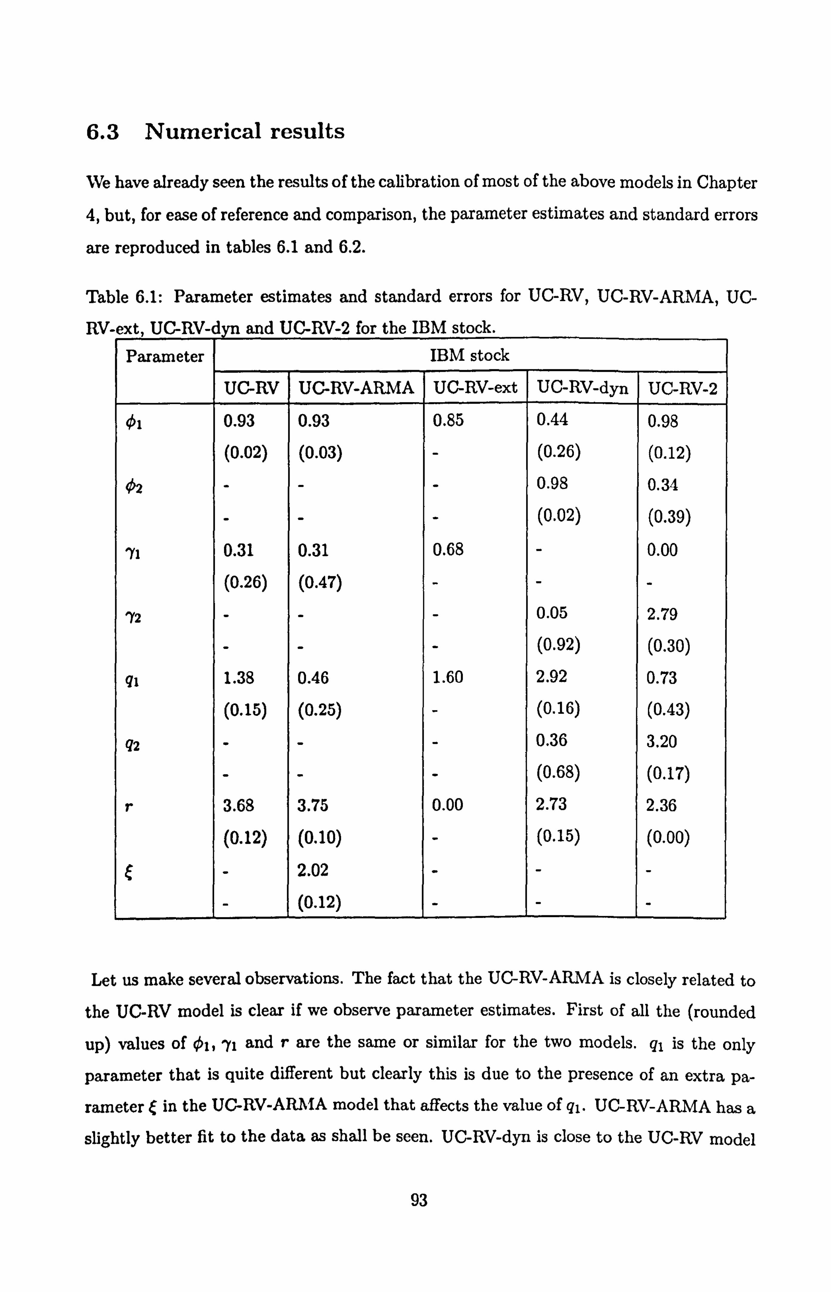
6.3 Numerical results

We have already seen the results of the calibration of most of the above models in Chapter

4, but, for ease of reference and comparison, the parameter estimates and standard errors

are reproduced in tables 6.1 and 6.2.

Table 6.1: Parameter estimates and standard errors for UC-RV, UC-RV-ARMA, UC-

RV-ext, UC-RV-dyn and UC-RV-2 for the IBM stock. Parameter IBM stock

UC-RV UC-RV-ARMA UC-RV-ext UC-RV-dyn UC-RV-2

O1 0.93 0.93 0.85 0.44 0.98 (0.02) (0.03) - (0.26) (0.12)

02 - - - 0.98 0.34

- - - (0.02) (0.39)

ryl 0.31 0.31 0.68 - 0.00

(0.26) (0.47) - - -

ry2 - - - 0.05 2.79

- - - (0.92) (0.30)

ql 1.38 0.46 1.60 2.92 0.73

(0.15) (0.25) - (0.16) (0.43)

q2 - - - 0.36 3.20

- - - (0.68) (0.17)

r 3.68 3.75 0.00 2.73 2.36

(0.12) (0.10) - (0.15) (0.00)

- 2.02 - - -

- (0.12) - - -

Let us make several observations. The fact that the UC-RV-ARMA is closely related to

the UC-RV model is clear if we observe parameter estimates. First of all the (rounded

up) values of 01, 'yi and r are the same or similar for the two models. ql is the only

parameter that is quite different but clearly this is due to the presence of an extra pa-

rameter C in the UC-RV-ARNIA model that affects the value of q1. UC-RV-ARMA has a

slightly better fit to the data as shall be seen. UC-RV-dyn is close to the UC-RV model

93

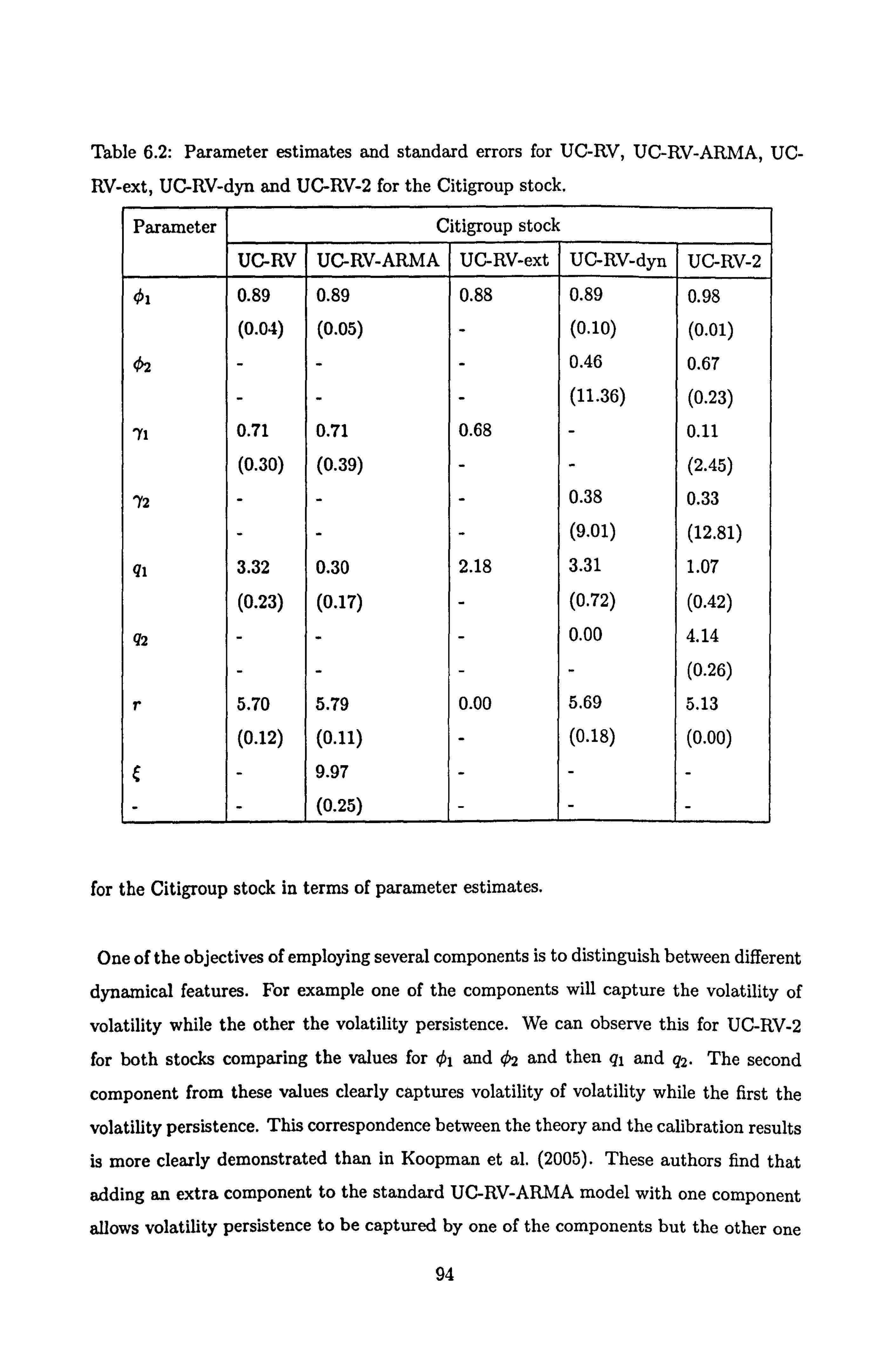
Table 6.2: Parameter estimates and standard errors for UC-RV, UC-RV-ARMA, UC-

RV-ext, UC-RV-dyn and UC-RV-2 for the Citigroup stock.

Parameter Citigroup stock

UC-RV UC-RV-ARMA UC-RV-ext UC-RV-dyn UC-RV-2

O1 0.89 0.89 0.88 0.89 0.98

(0.04) (0.05) - (0.10) (0.01)

02 - - - 0.46 0.67

- - - (11.36) (0.23)

ryl 0.71 0.71 0.68 - 0.11

(0.30) (0.39) - - (2.45)

72 - - - 0.38 0.33

- - - (9.01) (12.81)

ql 3.32 0.30 2.18 3.31 1.07

(0.23) (0.17) - (0.72) (0.42)

q2 - - - 0.00 4.14

- - - - (0.26)

r 5.70 5.79 0.00 5.69 5.13

(0.12) (0.11) - (0.18) (0.00)

- 9.97 - - -

- - (0.25) - - -

for the Citigroup stock in terms of parameter estimates.

One of the objectives of employing several components is to distinguish between different

dynamical features. For example one of the components will capture the volatility of

volatility while the other the volatility persistence. We can observe this for UC-RV-2

for both stocks comparing the values for 01 and 02 and then ql and q2. The second

component from these values clearly captures volatility of volatility while the first the

volatility persistence. This correspondence between the theory and the calibration results

is more clearly demonstrated than in Koopman et al. (2005). These authors find that

adding an extra component to the standard UC-RV-ARMA model with one component

allows volatility persistence to be captured by one of the components but the other one

94

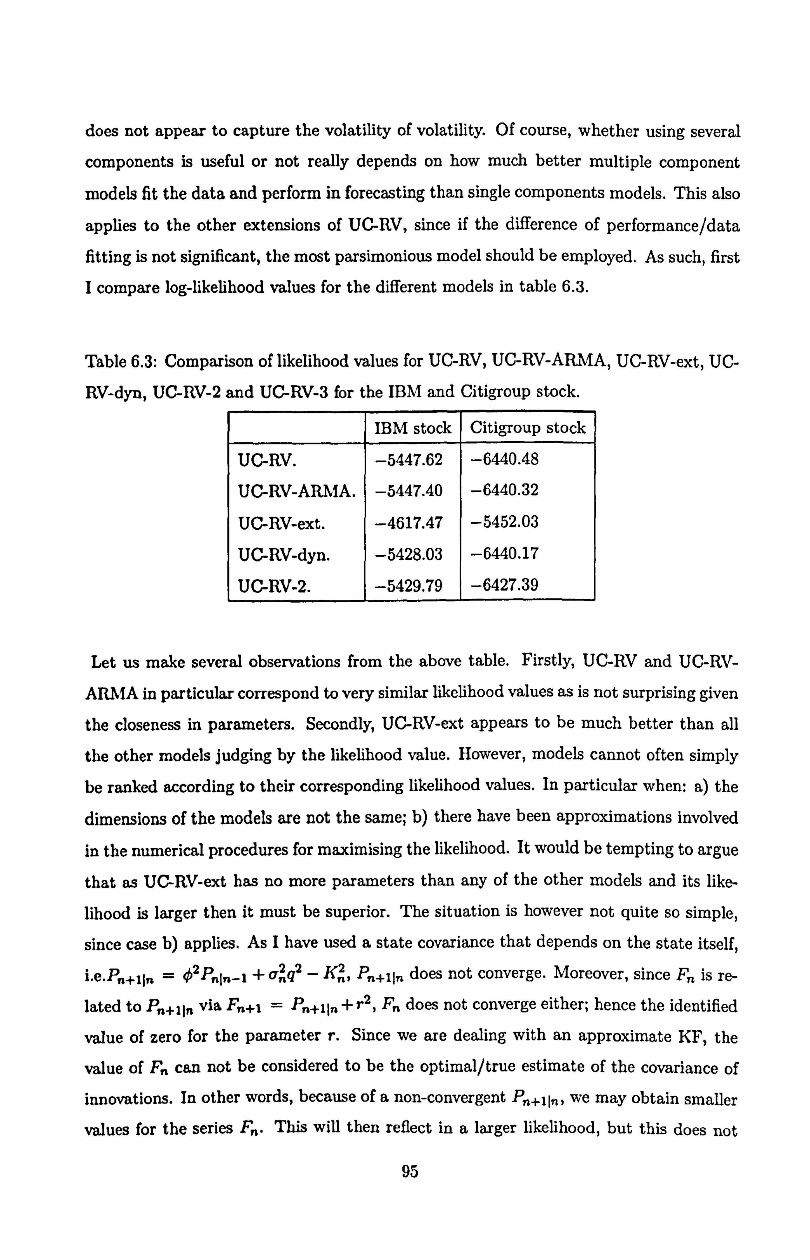
does not appear to capture the volatility of volatility. Of course, whether using several

components is useful or not really depends on how much better multiple component

models fit the data and perform in forecasting than single components models. This also

applies to the other extensions of UC-RV, since if the difference of performance/data

fitting is not significant, the most parsimonious model should be employed. As such, first

I compare log-likelihood values for the different models in table 6.3.

Table 6.3: Comparison of likelihood values for UC-RV, UC-RV-ARMA, UC-RV-ext, UC-

RV-dyn, UC-RV-2 and UC-RV-3 for the IBM and Citigroup stock.

IBM stock Citigroup stock

UC-RV. -5447.62 -6440.48 UC-RV-ARhMA. -5447.40 -6440.32

UC-RV-ext. -4617.47 -5452.03 UC-RV-dyn. -5428.03 -6440.17 UC-RV-2. -5429.79 -6427.39

Let us make several observations from the above table. Firstly, UC-RV and UC-RV-

ARMA in particular correspond to very similar likelihood values as is not surprising given

the closeness in parameters. Secondly, UC-RV-ext appears to be much better than all

the other models judging by the likelihood value. However, models cannot often simply

be ranked according to their corresponding likelihood values. In particular when: a) the

dimensions of the models are not the same; b) there have been approximations involved

in the numerical procedures for maximising the likelihood. It would be tempting to argue

that as UC-RV-ext has no more parameters than any of the other models and its like-

lihood is larger then it must be superior. The situation is however not quite so simple,

since case b) applies. As I have used a state covariance that depends on the state itself,

i. e. Pn+tin = 0ZPnIn-1 + Q2; 92 - Kn, Pn+11n does not converge. Moreover, since Fn is re-

lated to P, a+1 in via Fn+1 = Pn+I In + r2, Fn does not converge either; hence the identified

value of zero for the parameter r. Since we are dealing with an approximate KF, the

value of F� can not be considered to be the optimal/true estimate of the covariance of

innovations. In other words, because of a non-convergent P, i+11,,, we may obtain smaller

values for the series F, This will then reflect in a larger likelihood, but this does not

95

give any information on the actual variance of innovations. So although for UC-RV-ext

the likelihood may be larger than for the other models, it is the actual innovations that

will really show how good the model is.

As an example of case a) in the previous paragraph, let us take the UC-RV and UC-

RV-ARMA models for example. UC-RV is contained in UC-RV-ARMA. In other words

UC-RV-AR. MA is an extension of UC-RV and so UC-RV-ARMA has an `unfair advantage'

over UGRV. In usual statistical procedures it is verified if the difference in likelihood

values is significant enough to warrant using the more complex model structure of UC-

RV-ARIA over UC-RV. When models are nested this is done by making use of the F-test

which specifies that some function of the difference in likelihood values3 is X2 distributed

with degrees of freedom equal to the difference in the number of estimated parameters4.

If the value of this function is less that some critical value, then the difference in likelihood

values is not significant. This test was carried out for the UGRV and UC-RV-ARMA

models and the outcome was that the difference in likelihood values between these mod-

els was not significant for both stocks. The F-test was further carried for comparing the

UGRV and UC-RV-dyn models leading to the same conclusion for the Citigroup stock.

Also for the Citigroup stock, the difference in likelihood values between the UC-RV and

UC-RV-2 models was insignificant5, although clearly this difference is greater than the

difference between the UGRV and UC-RV-dyn models. For the IBM stock however the

situation was not so clear cut. For UGRV and UGRV-dyn, the null hypothesis of no

statistical significance in the difference in likelihood values between these models was

rejected with 95% certainty. Furthermore, for the UGRV and UC-RV-2 models it was 'More precisely the difference in the values of some functional form that here I choose to be the

likelihood function. "A criterion for choosing between non-nested models is Akaike's information theoretic criterion (AIC)

Akaike (1972) and Akaike (1974). Consider the function for a given model M

A(M) = -g[-Clog + dM] (6.6)

where dM is the dimension of the model and LI09 is the log-likelihood function for model M. The AIC

chooses amongst models that minimise A. $Although Barndorf-Nielsen and Shephard (2002) display likelihood values for UC-RV-ARMA models

with one, two and three components, they do not carry out significance tests. Instead these authors

compare performance in terms of the Box-Pierce statistic and conclude that two or three components lead to an acceptable statistic value whereas for one it is too large.

96

also rejected, but only with 90% certainty. Arguably, a 90% confidence interval is not

good enough.

Before coming to some conclusion, let us compare the values of Lf ((4.24) with Q2 =

onin_11 where n is the index for a day) for the several models as in previous chapters.

We do this for two reasons: a) comparing likelihood values can be non-informative and

b)L f, which is a function of the actual innovations alone, as opposed to the likelihood

which is a function of both the innovations and their variance, may have more of a direct

interpretation. For these reasons, in table 6.4 1 compare loss function values for the five

models based on the actual innovations: Observing table 6.4, we can see that comment

Table 6.4: Comparison of loss functions for UC-RV, UC-RV-ARMA, UC-RV-ext, UC-

RV-dyn and UC-RV-2 for the IBM and Citigroup stocks.

IBM stock UC-RV UC-RV-ARMA UC-RV-ext UC-RV-dyn UC-RV-2

18.73 18.73 23.53 18.35 18.36

Citigroup stock

UC-RV UC-RV-ARMA UC-RV-ext UC-RV-dyn UC-RV-2

53.61 53.61 66.75 53.61 52.86

b), on the mistake of simplistic ranking of models according to likelihood values, applies:

if we take UC-RV-ext it has a significantly larger likelihood value than the other models

but in terms of the actual observations it is the worst model for this forecasting horizon.

Let us recall that for the procedures of Chapter 4 it was comparable to the standard

UC-RV model. However for both a short and a medium-term horizon for the specific

forecasting procedures in chapters 5 and 6, this model does not perform very well (as

shown in tables 5.3 and 6.4). This could be due to the approximations involved in its

calibration as explained in point 3) of this chapter. Whatever the reasons are, this ob-

servation concurs with Jones (2003), and references therein, that also find unfavourable

"evidence" towards a square-root specification of the form of the transition equation of

UC-RV-ext. In fact Jones (2003) goes so far as to reject this model in favour of other SV

models'. *It should be pointed out that the context of this rejection is somewhat different from the one here.

97

As before, let us compare the models statistically using the same significance test for the

MSE as that of the previous chapters. The standard UC-RV model will be used as the

benchmark model for the comparison. UC-RV-2 is consistently better7 than UC-RV and

this difference is statistically significant to any standard significance level. On the other

hand, UC-RV-ext is consistently and significantly worse than UC-RV. Clearly the ARMA

component model is in real terms no better than the standard AR component model (the

difference in the two is indistinguishable due to the rounding up of decimals). The fact

that UC-RV-dyn is closely related to the UC-RV model, in terms of parameter estimates

for the Citigroup stock, is clearly demonstrated by a close forecasting performance (due

to the rounding up of decimals the difference is indistinguishable)8. However, for the

IBM stock the difference in loss function values between the UC-RV-dyn and UC-RV

models is statistically significant.

6.4 Conclusion

In this chapter five UC-RV-type models have been presented and issues related to their

characteristics and estimation procedures have been commented on. The calibration

results of the five models have been displayed and then the models have been compared

in terms of their fit of the data and forecasting performance. In summary, the two-state

models are statistically significantly better than the one-state models for the IBM stock,

but not necessarily for the Citigroup stock. Given this disparity, fundamentally it is a

matter of judgement whether the superior forecasting performance of a more complex

two-state model, warrants being employed, as opposed to a more parsimonious one-state

model. This is mainly due to the fact that the former is likely to involve a significant

amount more of computation time in the calibration. Finally I also conclude that the

standard UC-RV model with a Feller extension does not perform very well for the short

and medium-term horizon forecasting procedures of chapters 5 and 6.

In the setup of Jones (2003) the model that is rejected includes a square-root specification for the spot

price dynamics with correlation with the volatility dynamics, with the objective of pricing options. BAs is the case in the other chapters. °These results are in stark contrast to those in Chapter 4 where UC-RV-dyn is better in five out of

six cases than UC-RV and Chapter 5 where UC-RV-dyn is better for both stocks (see table 5.3).

98

Contributions and further work

This thesis has covered background theory related to financial modelling with an emphasis

on linear state model estimation and prediction. This theory has successfully been applied

in the estimation of models using high frequency stock price data. We also demonstrated

how implied volatility measurements could be incorporated into a linear state space

model. The main contributions from this present work are as follows:

-I have presented an overview of fundamental developments in the theory of financial

modelling.

-I have described several modelling and statistical procedures of relevance to the

applications of this thesis as well as the broader subject of financial modelling.

- From Chapter 41 conclude that filtering measurement noise improves volatility

estimation and prediction for the data set used in this study.

-I have compared different prediction methods for the same forecasting horizon for

UC-RV, LARCH and constant volatility models. I conclude that for the UC-RV-

type models the scaling method worked the best, for GARCH-type models the

multi-step method worked the best and for the constant volatility models, it was

the one-day method that worked best.

-I have found that including implied volatility measurements brought improvement

to the forecasting performance of UC-RV-type models under consideration.

-I have found that for the dataset and modelling procedures under consideration,

none of the four UC-RV-type model extensions to the standard UC-RV model used

in this thesis performed significantly better than it for a short-term forecast horizon.

However, the two-state models did bring some improvement.

99

A significant numerical experience has been gained in development, calibration and

forecasting using linear volatility models during this project. The details of the numerical

studies as well as the software developed will form a useful resource for further empirical

work. I expect further work to take two main directions. The first is the use of high

frequency data to calibrate linear state space models to model the covariance matrix of

a basket of stocks. This will present new challenges as it is well known that correlations

between stocks have little predictability. The second direction would be to extend a UC-

RV-type model to price options on relevant stocks. In this way we would seek a model

that would explain the `smile' as well as fitting the high frequency return data well as

well.

100

Notation

]E(X) the expectation of a random variable X

Var(X) the variance of a random variable X

IN the identity matrix of size N

i. i. d. independently and identically distributed

NID normal and independently distributed

Ac the complement of the set A

A' the transpose of matrix A

tr(A) the trace of matrix A

RAISE Root mean squared error

SDE stochastic differential equation

h. o. t. higher order terms

w. l. o. g. without loss of generality

B(") or IV(. ) Brownian motion

101

Appendix A

Quasi-Maximum Likelihood Estimation

Here I seek to show the details behind calculating the covariance error matrix, and from

this the standard errors, of a possibly misspecified multivariate hidden state model.

Consider the log-likelihood function,

TT Llog(yT" I .)_-Z log I Fn 1-Z vnFn lvn, (A. 1)

n=I n=1

where _v,, are the innovations, and F� are their variance, B is the vector of unknown

parameters, of dimension m, say. The innovations are defined as,

Vom. -Z , n_I-Cý'

where, as given in (2.28) and (2.29), yn are the observations, d and Z are a constant

vector and matrix, respectively, and ,,, _1 are the estimates of the hidden state. The

maximisation of (A. 1) is equivalent to maximising the probability of the outcome of the

set of observations.

We see from (A. 1) that the innovations with a smaller variance are given more weight in

the optimisation. The parameter vector which maximises the likelihood of the observa-

tions is called the maximum likelihood estimate, 6. If the sample size is sufficiently large

and under certain regularity conditions we have,

g _.., D N(B , T-'I-1(B)), (A. 2)

where B denotes the true parameter vector. The matrix I(9) is denoted the information

matrix and is based on derivatives of the likelihood function w. r. t. the parameter vector.

102

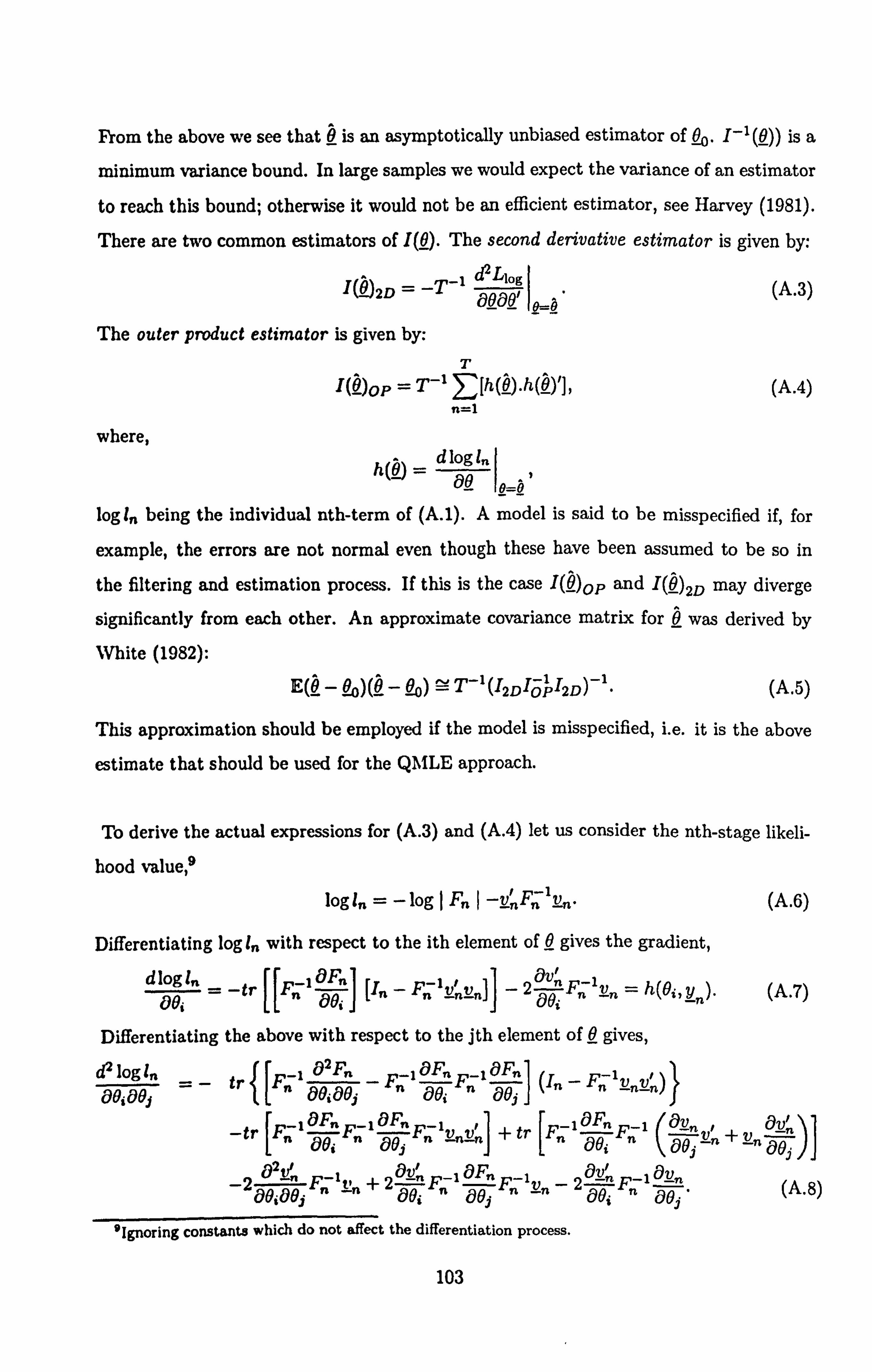
From the above we see that B is an asymptotically unbiased estimator of 90.1 ' (B)) is a

minimum variance bound. In large samples we would expect the variance of an estimator

to reach this bound; otherwise it would not be an efficient estimator, see Harvey (1981).

There are two common estimators of I (9). The second derivative estimator is given by:

I( )2D = -T-1 ` Llog +

(A. 3) aeae I ý-B '

The outer product estimator is given by: T

I(2)op = T-1 E[h(B). h(9)'], (A. 4) n=1

where,

h(j _ dlogl�

62

10=0.1

log I� being the individual nth-term of (A. 1). A model is said to be misspecified if, for

example, the errors are not normal even though these have been assumed to be so in

the filtering and estimation process. If this is the case I(9)Op and 4)2D may diverge

significantly from each other. An approximate covariance matrix for B was derived by

White (1982):

-0 , ý. -i (IZDIiPI2D)-1 (A. 5) E(ä - -0o)(e -0

This approximation should be employed if the model is misspecified, i. e. it is the above

estimate that should be used for the QDMLE approach.

To derive the actual expressions for (A. 3) and (A. 4) let us consider the nth-stage likeli-

hood value, 9

login = -log Fn I -v_nFn lv_n" (A. 6)

Differentiating log l,, with respect to the ith element of 9 gives the gradient,

dlogln _ -tr If Fn '50 -j [In - Fn 1tJnvný]

- 2avnFn lvn = h(ei, yn)" 00 iJ Doi

(A. 7)

i Differentiating the above with respect to the jth element of 9 gives,

d2109 l tri [Fn1 t Fn1 OF, ýIn-Fn1vnz1'n)} -Fn, ae 89; 88 801 j`; ;J

(ä_vn + 1 [F-10 n F, -,

8Fn F- lv+ tr FýF'r_ 1 -tr n_1 Fn n _nvý -n 7 - J1 n

0v D 0 , a8; ,, 00j Öaß ' lJ

-2 02" Fn ltvn +2av"Fn 1ÖFnFn 1vn

- 2ÖvnF'n 1ä_vn

aeiae; aei 06j aei ae (A. 8)

; 9ignoring constants which do not affect the differentiation process.

103

Summing over n in (A. 8) and dividing by T we have the ij-th element of the second

derivative estimate of the information matrix as in (A. 3). If the model is correctly spec-

ified the above simplifies considerably. The derivatives of F, ' and vn can be found using

a set of recursions that run in parallel with the KF. See (Harvey, 1989, p. 140-143), for

example, for details. The presentation of the results for the diagonals of the covariance

matrix in (A. 5) using (A. 3) and (A. 4) and the information matrix (A. 8) are given in the

numerical results sections of Chapter 4,5 and 6.

For the GARCH-type models similar derivations of the first and second derivatives of

the likelihood can be carried out. The expressions however are greatly simplified as the

c(n) terms, corresponding to the v above, are not functions of the parameters10. For the

GARCH-type models of Chapter 4, the calibration is based on the Student t-distribution.

This means that at least in what concerns non-normality, the GARCH-type models are

correctly specified. Because I assume these models are correctly specified, standard max-

imum likelihood is employed. This in turn means that the covariance matrix estimate is

found from (A. 2), with 1(0) calculated from either (A. 3) or (A. 4).

1°An exception to this would be when the model the CARCH residuals are regressed on a number of

explanatory variables and the regression parameters are found via the likelihood, which is not the case

here.

104

Appendix B

Numerical computations for the QMLE standard errors

In this appendix I give the programs and a guide to the computer programs written for

the MATLAB environment. These programs compute the standard errors of UC-RV-

type and LARCH-type models. Although the programs themselves also form a part of

this appendix, for practical reasons these are included separately on a CD-ROM that

has been attached with the thesis. The programs have self-explanatory documentation

so this present guide will be limited in content.

In the table below there is a short guide to the relevant programs:

Tah1e 13.1 ! Programs for the UC-RV and GARCH-tvue models.

Program name Model Initialisation

likefRelstep UC-RV stationary values

UClikefreeCderl UC-RV-2 stationary values

UClikefreeCderO UC-RV-2 diffuse prior (k = 1000)

ARA1AlikefreeCder UC-RV-AMIA stationary values

twoDgammalikefreeCder UC-RV-dyn stationary values

UCIMMPlikefreeCder UC-RV-IV stationary values

IfewmatMML EWNIA(-t) sample mean 1fGarchtML LARCH(-t) stationary values

lfGarchtLEVNIL LARCH-GJR(-t) sample mean

The material in the previous appendix as well as in section 4.5.3 explain how the standard

errors are calculated for each model. It should be pointed out that I found that the UC-

105

RV-2 model with a diffuse initialisation led to better forecasting performance for both

stocks. Hence the inclusion of the routine for this initialisation in the above list of

routines.

106

Acknowledgements

First of all I owe a debt of gratitude to my supervisor Dr. Paresh Date for all his hard

work, dedication and advice throughout my PhD. If I believed in luck I would say that

I am extremely lucky to have had such a great advisor. I would also like to thank my

second supervisor Dist. Prof. Gautam Mitra for his support and contributions.

My two examiners Dr. Yuanhua Feng and Dr. Kerning Yu are to be thanked for their

careful consideration of this present work.

I would like to thank my family, in particular my parents, for their support and interest

in the undertaking.

Thanks also go to Brunel University associated staff and PhD colleagues such as Ro-

georar Mamon, Christina Erlwein and Keming Yu, Kay Lawrence, Bev Curr and Neil

Thrner.

Finally, I am grateful to my Lord and Saviour Jesus Christ for His faithfulness and

goodness to me during the course of my PhD and indeed my whole life.

107

Bibliography

Ait-Sahalia, Y., Mykland, P. A., Zhang, L., 2005. How often to sample a continuous-time process in the presence of market microstructure noise. Review of Financial Studies

18 (2), 351-416.

Akaike, H., 1972. Use of an information theoretic quantity for statistical model identifi-

cation. Proceedings of the Fifth Hawaii International Conference on System Sciences.

North Hollywood, California (Western Periodicals), 249-250.

Akaike, li., 1974. A new look at statistical-model identification. IEEE Transactions on

Automatic Control 19 (6), 716-723.

Alizadeh, S., Brandt, M. WV., Diebold, F. X., 2002. Range-based estimation of stochastic

volatility models. Journal of Finance 57 (3), 1047-1089.

Amin, K., Ng, V., 1993. Option valuation with systematic stochastic volatility. The

Journal of Finance 48 (3), 881-910.

Andersen, T., Benzoni, L., Lund, J., 2002. An empirical investigation of continuous-time

equity return models. The Journal of Finance 57 (3), 1239-1284.

Andersen, T. G., 2000. Some reflections on analysis of high-frequency data. Journal of Business and Economic Statistics 18 (2), 146-153.

Andersen, T. G., Bollerslev, T., 1997. Intraday periodicity and volatility persistence in

financial markets. Journal of Empirical Finance 4 (2-3), 115-158.

Andersen, T. G., Bollerslev, T., 1998. Answering the skeptics: yes, standard volatility

models do provide accurate forecasts. International Economic Review 39 (4), 885-905.

Andersen, T. G., Bollerslev, T., Diebold, F. X., Ebens, H., 2001. The distribution of

realized stock return volatility. Journal of Financial Economics 61 (1), 43-76.

108

Andersen, T. G., BollersIev, T., Diebold, F. X., Labys, P., 1999a. Exchange rate returns

standardized by realized volatility are (nearly) gaussian. Working paper available at

http: //www. smartquant. com/references/Volatility/voll. pdf, [2 Febuary 20071.

Andersen, T. G., Bollerslev, T., Diebold, F. X., Labys, P., 2003. Modeling and forecasting

realized volatility. Econometrica 71 (2), 579-625.

Andersen, T. G., Bollerslev, T., Lange, S., 12 1999b. Forecasting financial market volatil-

ity: sample frequency vis-a-vis forecast horizon. Journal of Empirical Finance 6 (5),

457-477.

Anderson, B. D. 0., Moore, J. B., 1979. Optimal filtering. Prentice-Hall, London.

Andersson, P. J., Oberg, A., Guhr, T., 2005. Power mapping and noise reduction for

financial correlations. Acta Physics Polonica B 36 (9), 2611-2619.

Andreou, E., Ghysels, E., 2002. Rolling-sample volatility estimators: some new theoret-

ical, simulation, and empirical results. Journal of Business and Economic Statistics

20 (3), 363-376.

Areal, N., Taylor, S., 2002. The realized volatility of FTSE-100 futures prices. Journal of

Futures Markets 22 (7), 627-648.

Baadsgaard, M., Madsen, If., Nielsen, J., 2001. Estimating and testing an exponential-

affine term structure model by nonlinear filtering. Technical University of Denmark-

Manuscript. Available at http: //citeseer. ist. psu. edu/234561. htm1, [5 Febuary 2007].

Baba, Y., Engle, R., Kraft, D., Kroner, K., 1991. Multivariate simultaneous general-

ized ARCH. Department of Economics, University of California, San Diego. Discussion

paper.

Bachelfer, L., 1900. Theorie de la speculation. Annales Scientifiques de 1'Ecole Normale

Superieure Ser. 3 17,21-86.

Bakshi, C., Cao, C., Chen, Z., 1997. Empirical performance of alternative option pricing

models. Journal of Finance 52 (5), 2003-2049.

Ball, C., Roma, A., 1994. Stochastic volatility option pricing. The Journal of Financial

and Quantitative Analysis 29 (4), 589-607.

109

Bandi, F. M., Russell, J. R., 2006. Separating microstructure noise from volatility. Journal

of Financial Economics 79 (3), 655-692.

Barndorfl-Nielsen, O. E., Shephard, N., 2001. Non-Gaussian Ornstein-Uhlenbeck-based

models and some of their uses in financial economics. Journal of the Royal Statistical

Society Series B-Statistical Methodology 63,167-207.

Barndorif-Nielsen, 0. E., Shephard, N., 2002. Econometric analysis of realized volatility

and its use in estimating stochastic volatility models. Journal of the Royal Statistical

Society Series B-Statistical Methodology 64,253-280.

Banndorf Nielsen, 0. E., Shephard, N., 2004. Econometric analysis of realized covari-

ation: high frequency based covariance, regression, and correlation in financial eco-

nomics. Econometrica 72 (3), 885-925.

Barone-Adesi, C., Whaley, ß., 1987. Efficient analytic approximation of American option

values. The Journal of Finance 42 (2), 301-320.

Basel, C., January 1996. Basel Committee on banking supervision. Amend-

ment to the capital accord to incorporate market risks. Available at

http: //www. bis. org/publ/bcbs24. pdf, [6 Febuary 2007].

Bates, D. S., 1996. Jumps and stochastic volatility: exchange rate processes implicit in

deutsche mark options. Review of Financial Studies 9 (1), 69-107.

Bauwens, L., Laurent, S., Rombouts, J. V. K., 2006. Multivariate GARCH models: a

survey. Journal of Applied Econometrics 21 (1), 79-109.

Bhar, IL, Chiarella, C., Runggaldier, WV., 2004. Inferring the forward looking equity risk

premium from derivative prices. Studies in Nonlinear Dynamics & Econometrics 8 (1),

1-24.

Bjork, T., 2004. Arbitrage theory in continuous time. Oxford University Press, Oxford.

Black, F., Scholcs, M., 1973. Pricing of options and corporate liabilities. Journal of Po-

litical Economy 81 (3), 637-654.

Blair, B., Poon, S., Taylor, S., 2001. Forecasting S&P 100 volatility: the incremental

information content of implied volatilities and high frequency index returns. Journal

of Econometrics 105 (1), 5-26.

110

Blake, D., Cairns, D., Dowd, K., August 2000. Extrapolating VaR by the square-root

rule. Financial Engineering News 17,3,7.

Bollerslev, T., 1986. Generalized autoregressive conditional heteroskedasticity. Journal of Econometrics 31 (3), 307-327.

Bollerslev, T., 1987. A conditionally heteroskedastic time series model for speculative

prices and rates of return. The Review of Economic Statistics 69 (3), 542-547.

Bollerslev, T., 1990. Modelling the coherence in short-run nominal exchange rates: a

multivariate generalized ARCH model. The Review of Economics and Statistics 72 (3),

498-505.

Bollerslev, T., Baillie, R., Mikkelsen, H., 1996. Fractionally integrated generalized au-

toregressive conditional heteroskedasticity. Journal of Econometrics 74,3-30.

Bollerslev, T., Engle, R. F., Wooldridge, J. M., 1988. A capital asset pricing model with

time-varying covariances. Journal of Political Economy 96 (1), 116-131.

Bollerslev, T., Wooldridge, J. M., 1992. Quasi-maximum likelihood estimation and infer-

ence in dynamic models with time-varying covariances. Econometric Reviews 11 (2),

143-172.

Bollerslev, T., Zhou, H., 2002. Estimating stochastic volatility diffusion using conditional

moments of integrated volatility. Journal of Econometrics 109 (1), 33-65.

Brandimarte, P., 2002. Numerical methods in finance: a MATLAB-based introduction.

Wiley, New York.

Breidt, F., Crato, N., de Lima, P., 1998. The detection and estimation of long memory

in stochastic volatility. Journal of Econometrics 83 (1), 325-348.

Broyden, C., 1970. The convergence of a class of double-rank minimization algorithms.

Journal of the Institute of Mathematical Applications 6 (3), 76-90.

Buffington, J., Elliott, R., 2002. American options with regime switching. International

Journal of Theoretical and Applied Finance 5,497-514.

Campbell, J., Lo, A., MacKinley, A., 1997. The econometrics of financial markets. Prince-

ton University Press, Princeton, New Jersey.

111

Canina, L., Figlewski, S., 1993. The informational content of implied volatility. Review

of Financial Studies 6 (3), 659-681.

Carr, P., Geman, H., Madan, D. B., Yor, M., 2003. Stochastic volatility for Levy pro-

cesses. Mathematical Finance 13 (3), 345-382.

Carr, P., \Vu, L. R.., 2004. Time-changed Levy processes and option pricing. Journal of

Financial Economics 71 (1), 113-141.

Casals, J., Sotoca, S., 2001. The exact likelihood for a state space model with stochastic

inputs. Computers and Mathematics with Applications 42 (1), 199-209.

Chernov, M., Ghysels, E., 2000. A study towards a unified approach to the joint esti-

mation of objective and risk neutral measures for the purpose of options valuation.

Journal of Financial Economics 56 (3), 407-458.

Chesney, M., Scott, L., 1989. Pricing European currency options: a comparison of the

modified Black-Scholes model and a random variance model. The Journal of Financial

and Quantitative Analysis 24 (3), 267-284.

Chiras, D., Manaster, S., 1978. The information content of option prices and a test of

market efficiency. Journal of Financial Economics 6 (2), 213-234.

Christensen, B. J., Prabhala, N. R., 1998. The relation between implied and realized

volatility. Journal of Financial Economics 50 (2), 125-150.

Christoffersen, P., Diebold, F., Schuermann, T., 1998. Horizon problems and extreme

events in financial risk management. Economic Policy Review 4,109-118.

Christoffersen, P., Jacobs, K., 2004. Which LARCH model for option valuation? Man-

agement Science 50 (9), 1204-1221.

Comte, F., Renault, E., 1998. Long memory in continuous-time stochastic volatility mod-

els. Mathematical Finance 8 (4), 291-323.

Cont, R., da Fonseca, J., 2002. Dynamics of implied volatility surfaces. Quantitative

Finance 2 (1), 45-60.

Cont, R., Tankov, P., 2004. Financial modelling with jump processes. Chapman & Hall,

Boca Raton, Florida.

112

Cox, J., 1975. Notes on option pricing I: constant elasticity of diffusions. Unpublished

draft, Stanford University.

Cox, J., Ingersoll, J. E., Ross, S. A., 1985a. An intertemporal general equilibrium model

of asset prices. Econometrica 53 (2), 363-384.

Cox, J., Ingersoll, J. E., Ross, S. A., 1985b. A theory of the term structure of interest-

rates. Econometrica 53 (2), 385-407.

Cox, J., Ross, S., Rubinstein, M., 1979. Option pricing: a simplified approach. Journal

of Financial Economics 7,229-263.

Danielsson, J., Richard, J., 1993. Accelerated Gaussian importance sampler with appli-

cation to dynamic latent variable models. Journal of Applied Econometrics 8,153-173.

Day, T., Lewis, C., 1992. Stock market volatility and the information content of stock index options. Journal of Econometrics 52 (1), 267-287.

Dempster, A., Laird, N., Rubin, D., 1977. Maximum likelihood from incomplete data via

the EM algorithm. Journal of the Royal Statistical Society. Series B (Methodological)

39 (1), 1-38.

Derman, E., Kan!, I., 1994. Riding on a smile. Risk 7 (2), 32-39.

Drost, F., Nijman, T. E., 1993. Temporal aggregation of GARCH processes. Economet-

rica: Journal of the Econometric Society 61 (4), 909-927.

Drost, F. C., Werker, B. J. M., 9 1996. Closing the GARCH gap: continuous time

GARCH modeling. Journal of Econometrics 74 (1), 31-57.

Duan, J., 1995. The GARCH option pricing model. Mathematical Finance 5,13-32.

Duffie, D., Singleton, K. J., 1993. Simulated moments estimation of Markov-models of

asset prices. Econometrics 61 (4), 929-952.

Dupire, B., 1994. Pricing with a smile. Risk 7 (1), 18-20.

Durbin, J., Koopman, S., 2001. Time series analysis by state space methods. Oxford

University Press, Oxford.

113

Eatwell, J., Milgate, M., Newman, P., 1994. The New Palgrave: Finance. Macmillan,

Basingstoke; London.

Ederington, L., Guan, `V., 2002. Measuring implied volatility: is an average better?

Which average? Journal of Futures Markets 22 (9), 811-837.

Elliott, R., Aggoun, L., Moore, J., 1995. Hidden Markov models: estimation and control.

Springer-Verlag, New York.

Elliott, it, Chan, L., Siu, T., 2005. Option pricing and Esscher transform under regime

switching. Annals of Finance 1 (4), 423-432.

Engle, R., 2000. The econometrics of ultra-high-frequency data. Econometrica 68 (1),

1-22.

Engle, R., 2002. Dynamic conditional correlation: a simple class of multivariate gener-

alized autoregressive conditional heteroskedasticity models. Journal of Business and

Economic Statistics 20 (3), 339-350.

Engle, it, Bollerslev, T., 1986. Modelling the persistence of conditional variances. Econo-

metric Reviews 5 (1), 1-50.

Engle, R., Gonzalez-Rivera, G., 1991. Semiparametric ARCH Models. Journal of Business

& Economic Statistics 9 (4), 345-359.

Engle, R., Mustafa, C., 1992. Implied ARCH models from options prices. Journal of

Econometrics 52 (1), 289-311.

Engle, R. F., 1982. Autoregressive conditional heteroskedasticity with estimates of the

variance of United Kingdom inflation. Econometrica 50 (4), 987-1007.

Engle, R. F., Ding, Z., 2001. Large scale conditional covariance matrix: modeling,

estimation and testing, NYU Stern School of Business, New York. Working pa-

per available at http: //w4. stern. nyu. edu/finance/docs/WP/2001/pdf/wpa01029. pdf, [2 Febuary 20021.

Engle, R. F., Kroner, K., 1995. Multivariate simulataneous GARCH. Econometric Theory

11,122-150.

114

Eraker, B., 2004. Do stock prices and volatility jump? Reconciling evidence from spot

and option prices. The Journal of Finance 59 (3), 1367-1404.

Fama, E., 1970. Efficient capital markets: a review of theory and empirical work. The

Journal of Finance 25 (2), 383-417.

Figlewski, S., 1997. Forecasting volatility. Financial Markets Institutions and Instruments

6(l), 1-88.

Fisher, R., 1922. On the mathematical foundations of theoretical statistics. Philosoph-

ical Transactions of the Royal Society of London. Series A, Containing Papers of a

Mathematical or Physical Character 222,309-368.

Fisher, R., 1925. Theory of statistical estimation. Proceedings of the Cambridge Philo-

sophical Society 22 (5), 700-725.

Fleming, J., Kirby, C., 2003. A closer look at the relation between GARCH and stochastic

autoregressive volatility. Journal of Financial Econometrics 1 (3), 365-419.

Fleming, J., Ostdiek, B., Whaley, R., 1995. Predicting stock market volatility: a new

measure. Journal of Futures Markets 15 (3), 265-302.

Fletcher, R., 1970. A new approach to variable metric algorithms. The Computer Journal

13 (3), 317-322.

Forbes, C., Martin, G., Wright, J., 2002. Bayesian estimation of a stochas-

tic volatility model using option and spot prices, dept. of Econometrics

and Business Statistics, Monash University. Working paper available at

http: //www. buseco. monash. edu. au/depts/ebs/pubs/wpapers/2002/wp2-02. pdf,

[2 Febuary 2007].

Foster, D., Nelson, D., 1996. Continuous record asymptotics for rolling sample variance

estimators. Econometrica 64 (1), 139-174.

Fouque, J. P., Papanicolaou, G., Sircar, K. It., 2000. Derivatives in financial markets

with stochastic volatility. Cambridge University Press, Cambridge.

Gallant, A., Tauchen, G., 1996. Which moments to match. Econometric Theory 12 (4),

657-81.

115

Geman, H., Madan, D. B., Yor, M., 2001. Time changes for Levy processes. Mathematical

Finance 11 (1), 79-96.

Ceske, R., 1979. The valuation of compound options. Journal of Financial Economics

7 (1), 63-81.

Geweke, J., Porter-Hudak, S., 1983. The estimation and application of long memory time

series. Journal of Time Series Analysis 4,221-238.

Glosten, L., Jaganathan, R., Runkle, D., 1993. On the relation between the expected

value and the volatility of the nominal excess return on stocks. The Journal of Finance

48 (5), 1779-1801.

Goldfarb, D., 1970. A family of variable-metric methods derived by variational means.

Mathematics of Computation 24 (109), 23-26.

Gonzalez-Rivera, G., Drost, F., 1999. Efficiency comparisons of maximum-likelihood-

based estimators in LARCH models. Journal of Econometrics 93 (1), 93-111.

Gordon, N., Salmond, D., Smith, A., 1993. Novel approach to nonlinear/non-Gaussian

Bayesian state estimation. Radar and Signal Processing, IEE Proceedings F 140 (2),

107-113.

Gourieroux, C., Monfort, A., Renault, E., 1993. Indirect inference. Journal of Applied

Econometrics 8,85-118.

Granger, C., 1980. Long memory relationships and the aggregation of dynamic models.

Journal of Econometrics 14,227-238.

Granger, C., Joyeux, R., 1980. An introduction to long-range time series models and

fractional differencing. Journal of Time Series Analysis 1 (1), 15-30.

Guo, D., 1996. The predictive power of implied stochastic variance from currency options.

Journal of Futures Markets 16 (8), 915-942.

Guo, D., 1998. The risk premium of volatility implicit in currency options. Proceedings

of the IEEE/IAFE/INFORMS Conference on Computational Intelligence for Financial

Engineering (1998), 224-251.

116

Cuo, X., Zhang, Q., 2004. Closed-form solutions for perpetual American put options with

regime switching. SIAMS Journal on Applied Mathematics 64 (6), 2034-2049.

Hakansson, N., 1971. Multi-period mean-variance analysis: toward a general theory of

portfolio choice. The Journal of Finance 26 (4), 857-884.

Hamilton, J. D., 1994. Time series analysis. Princeton University Press, Princeton, New

Jersey.

Hamilton, J. D., Susmel, R., 1994. Autoregressive conditional heteroskedasticity and

changes in regime. Journal of Econometrics 64 (1-2), 307-333.

Hansen, L., 1982. Large sample properties of Generalized Method of Moments estimators.

Econometrica 50 (4), 1029-1054.

Hansen, P., Lunde, A., 2005a. A forecast comparison of volatility models: does anything

beat a GARCH(1,1)? Journal of Applied Econometrics 20 (7), 873-889.

Hansen, P., Lunde, A., 2005b. A realized variance for the whole day based on intermittent

high-frequency data. Journal of Financial Econometrics 3 (4), 525-554.

Harrison, J., Pliska, S., 1981. Martingales and stochastic integrals in the theory of con-

tinous trading. Stochastic Processes and their Applications 11,215-260.

Hartley, H., 1958. Maximum likelihood estimation from incomplete data. Biometrics

14 (2), 174-194.

Harvey, A., 1998. Long memory in stochastic volatility. Butterworth-Heineman, Oxford,

forecasting Volatility in the Financial Markets.

Harvey, A., Ruiz, E., Shephard, N., 1994. Multivariate stochastic variance models. The

Review of Economic Studies 61 (2), 247-264.

Harvey, A. C., 1981. The Econometric Analysis of Time-series. Philip Allan, Oxford; New

York.

Harvey, A. C., 1989. Forecasting, structural time series models and the Kalman filter.

Cambridge University Press, Cambridge.

117

Heath, D., Jarrow, R., Morton, A., 1992. Bond pricing and the term structure of interest

rates: a new methodology for contingent claims valuation. Econometrica 60 (1), 77-

105.

Heston, S. L., 1993. A closed-form solution for options with stochastic volatility with

applications to bond and currency options. Review of Financial Studies 6 (2), 327-

343.

Heston, S. L., Nandi, S., 2000. A closed-form GARCH option valuation model. Review

of Financial Studies 13 (3), 585-625.

UßL

Holst, E., Thyregod, P., 1999. A statistical test for the mean squared error. Journal of

statistical computation and simulation 63 (4), 321-347.

Howison, S., Kelly, F., Wilmott, P., 1995. Mathematical models in finance. Chapman &

Hall, London.

Hull, J., White, A., 1987. The pricing of options on assets with stochastic volatilities.

Journal of Finance 42 (2), 281-300.

Ito, K., 1944. Stochastic integral. Proceedings of the Imperial Academy of Tokyo 20,

519-524.

Ito, K., 1951a. Multiple Wiener integral. Journal of the Mathematical Society of Japan

3 (1), 157-169.

Ito, K., 1951b. On stochastic differential equations. Memoirs of the American Mathemat-

ical Society 4,1-51.

Jackwerth, J., 1997. Generalized binomial trees. Journal of Derivatives 5,7-17.

Jacquier, E., Poison, N., Rossi, P., 1994. Bayesian analysis of stochastic volatility models.

Journal of Business & Economic Statistics 12 (4), 371-389.

Jacquier, E., Poison, N., Rossi, P., 1995. Models and prior distributions for multivariate

stochastic volatility. Graduate School of Business, University of ChicagoWorking paper

available at http: //ideas. repec. org/p/cir/cirwor/95s-18. html, [2 Febuary 2007].

James, J., Webber, N., 2000. Interest rate modelling. John Wiley & Sons, Chichester.

118

Jarque, C., Bera, A., 1987. A test for normality of observations and regression residuals.

International Statistical Review/Revue Internationale de Statistique 55 (2), 163-172.

Jobert, A., Rogers, L. C. G., 2006. Option pricing with Markov-modulated dynamics.

SIAM Journal on Control and Optimization 44 (6), 2063-2078.

Johnson, H., Shanno, D., 1987. Option pricing when the variance is changing. The Journal

of Financial and Quantitative Analysis 22 (2), 143-151.

Jones, C., 2003. The dynamics of stochastic volatility: evidence from underlying and

options markets. Journal of Econometrics 116 (1), 181-224.

Jorion, P., 1995. Predicting volatility in the foreign exchange market. Journal of Finance

50 (2), 507-528.

Kalman, R. E., 1960. A new approach to linear filtering and prediction problems. Journal

of Basic Engineering, Transactions AMSE Series D 82,35-45.

Kalman, R. E., Bucy, R. S., 1961. New results in linear filtering and prediction theory.

Journal of Basic Engineering, Transactions AMSE Series D 83,95-108.

Kendall, Id., 1953. The analysis of economic time series, part I: prices. Journal of the

Royal Statistical Society 96,11-25.

Kim, S., Shephard, N., Chib, S., 1998. Stochastic volatility: likelihood inference and

comparison with ARCH models. The Review of Economic Studies 65 (3), 361-393.

Kloeden, P., Platen, E., 2000. Numerical solution of stochastic differential equations.

Springer-Verlag, Berlin; New York; London.

Koopman, S. J., Hol, E., 2002. Stock index volatility forecasting with high frequency data.

Working paper available at http: //www. tinbergen. nl/discussionpapers/02068. pdf, [2

Febuary 2007).

Koopman, S. J., Jungbacker, B., Hol, E., 2005. Forecasting daily variability of the S&P

100 stock index using historical, realised and implied volatility measurements. Journal

of Empirical Finance 12 (3), 445-475.

Laloux, L., Cizeau, P., Bouchaud, J. P., Potters, M., 1999. Noise dressing of financial

correlation matrices. Physical Review Letters 83 (7), 1467-1470.

119

Lamoureux, C., Lastrapes, `V., 1993. The information content of implied volatilities.

Review of Financial Studies 6,659-681.

Latane, H., Rendleman, R., 1976. Standard deviations of stock price ratios implied in

option prices. The Journal of Finance 31 (2), 369-381.

Lintner, J., 1965. The valuation of risk assets and the selection of risky investments in

stock portfolios and capital budgets. Review of Economics and Statistics 47 (1), 13-37.

Liu, M., 2000. Modeling long memory in stock market volatility. Journal of Econometrics

99 (1), 139-71.

Ljung, L., 1987. System identification: theory for the user. Prentice-Hall, London.

Lo, A., 1986. Maximum likelihood estimation of generalized Ito processes with discretely

sampled data. Working paper available at http: //papers. nber. org/papers/TO059, [2

Febuary 2007].

Longstaff, F. A., Schwartz, E. S., 2001. Valuing American options by simulation: A

simple least-squares approach. Review of Financial Studies 14 (1), 113-147.

Lund, J., 1997. Non-linear Kalman filtering techniques for term-structure mod-

els. Aarhus School of Business, Aarhus University. Working paper available at

http: //www. jesperlund. com/thesis/essay5. pdf [5 Febuary 2007].

Madan, D., Carr, P., Chang, E., 1998. The Variance Gamma process and option pricing.

European Finance Review 2 (1), 79-105.

Madan, D. B., Seneta, E., 1990. The Variance Gamma (VG) model for share market

returns. Journal of Business 63 (4), 511-524.

Maheu, J., McCurdy, T., 2000. Identifying Bull and Bear markets in stock returns.

Journal of Business and Economic Statistics 18 (1), 100-112.

Mandelbrot, B., 1963. The variation of certain speculative prices. Journal of Business 36,

394-419.

Marcellino, M., Stock, J. H., Watson, M. W., 2006. A comparison of direct and iterated

multistep AR methods for forecasting macroeconomic time series. Journal of Econo-

metrics 135 (1-2), 499-526.

120

Marcucci, J., 2005. Forecasting stock market volatility with regime-switching GARCH

models. Studies in non-linear dynamics & econometrics 9 (4), 1-53.

Markowitz, If., Mar. 1952. Portfolio selection. Journal of Finance 7 (1), 77-91.

Martens, M., 2002. Measuring and forecasting S&P 500 index-futures volatility using

high-frequency data. Journal of Futures Markets 22 (6), 497-518.

Mayhew, S., Stivers, C., 2003. Stock return dynamics, option volume, and the information

content of implied volatility. Journal of Futures Markets 23 (7), 615-646.

URL http: //dx. doi. org/10.1002/fut. 10084

Meddahi, N., Renault, E., 1997. Aggregations and marginalization of

LARCH and stochastic volatility models, universite de Montreal, Centre de

recherche et developpement en economique. Unpublished paper available at

http: //www. sceco. umontreal. ca/publications/etext/9818. pdf, [2 Febuary 2007].

Meddahi, N., Renault, E., 2000. Temporal aggregation of volatility models. Unpublished

paper available at http: //www. cirano. qc. ca/pdf/publication/2000s-22. pdf, [2 Febuary

2007].

Melino, A., Turnbull, S., 1991. The pricing of foreign currency options. The Canadian

Journal of Economics 24 (2), 251-281.

Melino, A., Turnbull, S. M., 1990. Pricing foreign-currency options with stochastic volatil-

ity. Journal of Econometrics 45 (1-2), 239-265.

Merton, R., 1973a. An intertemporal capital asset pricing model. Econometrica 41 (5),

867-887.

Merton, R., 1973b. Theory of rational option pricing. The Bell Journal of Economics and

Management Science 4 (1), 141-183.

Merton, R., 1980. On estimating the expected return on the market. Journal of Financial

Economics 8 (4), 323-361.

Merton, R. C., 1976. Option pricing when underlying stock returns are discontinuous.

Journal of Financial Economics 3 (1-2), 125-144.

121

Mikosch, T., 1998. Elementary stochastic calculus with finance in view. Vol. 6. World

Scientific, Singapore; London.

Milne, F., 1995. Finance theory and asset pricing. Clarendon Press, Oxford.

Modigliani, F., Miller, M., 1958. The cost of capital, corporation finance and the theory

of investment. The American Economic Review 48 (3), 261-297.

Mossin, J., 1966. Equilibrium in a capital asset market. Econometrica 34 (4), 768-783.

Mossin, J., 1968. Optimal multiperiod portfolio policies. Journal of Business 41 (2), 215-

229.

Muller, U., Dacorogna, M., Dave, R., Pictet, 0., Olsen, R. B., Ward, J., 1993. Frac-

tals and intrinsic time -a challenge to econometricians. Working paper available at

http: //www. olsen. ch/research, [2 Febuary 2007].

Naik, V., 1993. Option valuation and hedging strategies with jumps in the volatility of

asset returns. Journal of Finance 48 (5), 1969-1984.

URL

Nelson, D. B., 1990. ARCH models as diffusion approximations. Journal of Econometrics

45 (1-2), 7-38.

Nelson, D. B., 1991. Conditional heteroskedasticity in asset returns -a new approach.

Econometrica 59 (2), 347-370.

Nicolato, E., Venardos, E., 2003. Option pricing in stochastic volatility models of the

Ornstein-Uhlenbeck type. Mathematical Finance 13 (4), 445-466.

Oomen, R., 2002. Modelling realized variance when returns are serially correlated. Work-

ing paper available at http: //www. warwick. ac. uk/staff/R. C. A. Oomen/, [2 Febuary

2007].

Owens, J., Steigerwald, D., 2005. Noise reduced realized volatility: a Kalman filter ap-

proach. Advances in Econometrics: Econometric Analysis of Economic and Financial

Time Series 20 (A), 211-230.

Patton, A., 2006. Volatility forecast comparison using imperfect volatility proxies. Work-

ing paper available at http: //ideas. repec. org/p/uts/rpaper/175. html, [2 Febuary 2007].

122

Plerou, V., Gopikrishnan, P., Rosenow, B., Amaral, L. A. N., Guhr, T., Stanley, H. E.,

2002. Random matrix approach to cross correlations in financial data. Physical Review

E 65 (6), 241-246.

Poison, N., Stroud, J., 2002. Bayesian inference for derivative prices. Bayesian Statistics

7,641-650.

Poon, S., Granger, C., 2003. Forecasting volatility in financial markets: a review. Journal

of Economic Literature 41 (2), 478-539.

Renault, E., 1997. Econometric models of option pricing errors. Advances in Economics

and Econometrics: Theory and Applications 3,223-278.

Renault, E., Touzi, N., 1996. Option hedging and implied volatilities in a stochastic

volatility model. Mathematical Finance 6 (3), 279-302.

Roberts, H., 1967. Statistical versus clinical prediction of the stock market. Tech. rep.,

Center for Research in Security Prices, University of Chicago.

Roll, R., 1977. An analytical valuation formula for unprotected American call options on

stocks with known dividends. Journal of Financial Economics 5 (2), 251-258.

Ross, S., 1976. The arbitrage theory of capital asset pricing. Journal of Economic Theory

13 (3), 341-360.

Rossi, A., Gallo, G. M., 2006. Volatility estimation via hidden markov models. Journal

of Empirical Finance 13 (2), 203-230.

Rubinstein, M., 1976. The valuation of uncertain income streams and the pricing of

options. The Bell Journal of Economics 7 (2), 407-425.

Rubinstein, M., 1985. Nonparametric tests of alternative option pricing models using all

reported trades and quotes on the 30 most active CBOE option classes from August

23,1976 through August 31,1978. The Journal of Finance 40 (2), 455-480.

Rubinstein, M., 1994. Implied binomial trees. The Journal of Finance 49 (3), 771-818.

Ruiz, E., 1994. Quasi-maximum likelihood estimation of stochastic volatility models. Journal of Econometrics 63 (1), 289-306.

123

Sabbatini, M., Linton, 0., 1998. A GARCH model of the implied volatility of the Swiss

market index from option prices. International Journal of Forecasting 14 (2), 199-213.

Samuelson, P., 1965. Proof that properly anticipated prices fluctuate randomly. Industrial

Management Review 6 (2), 41-49.

Samuelson, P., 1969. Lifetime portfolio selection by dynamic stochastic programming. The Review of Economics and Statistics 51 (3), 239-246.

Sandmann, G., Koopman, S. J., 1998. Estimation of stochastic volatility models via

Monte Carlo maximum likelihood. Journal of Econometrics 87 (2), 271-301.

Scalas, E., Gorenflo, R., Mainardi, F., 2000. Fractional calculus and continuous-time

finance. Physica A 284 (1-4), 376-384.

Schonbucher, P. J., 1999. A market model for stochastic implied volatility. Philosophi-

cal Transactions of the Royal Society of London Series A-Mathematical Physical and

Engineering Sciences 357 (1758), 2071-2092.

Scott, L., 1997. Pricing stock options in a jump-diffusion model with stochastic volatility

and stochastic interest rates: application of Fourier inversion methods. Mathematical

Finance 7,413-426.

Scott, L. 0., 1987. Option pricing when the variance changes randomly: theory, esti-

mation, and an application. Journal of Financial and Quantitative Analysis 22 (4),

419-438.

Shanno, D., 1970. Conditioning of quasi-Newton methods for function minimization.

Mathematics of Computation 24 (111), 647-656.

Sharpe, W., 1964. Capital asset prices: a theory of market equilibrium under conditions

of risk. The Journal of Finance 19 (3), 425-442.

Shephard, N., 1993. Fitting non-linear time series models, with applications to stochastic

variance models. Journal of Applied Econometrics 8,135-152.

Shephard, N., 2005. Stochastic volatility: selected readings. Oxford University Press,

Oxford.

Shreve, S., 2004. Stochastic calculus for finance II. Springer, New York.

124

Steele, J., 2003. Stochastic calculus and financial applications. Springer, New York; Lon-

don.

Stein, E. M., Stein, J. C., 1991. Stock-price distributions with stochastic volatility - an analytic approach. Review of Financial Studies 4 (4), 727-752.

Steinbach, M., 2001. Markowitz revisited: mean-variance models in financial portfolio

analysis. SIAM Review 43 (1), 31-85.

Szakmary, A., Ors, E., Kim, J., III, W. D., 2003. The predictive power of implied volatil- ity: evidence from 35 futures markets. Journal of Banking & Finance 27,2151-2175.

Taylor, S., 1982. Financial returns modeled by the product of two stochastic processes-a

study of the daily sugar prices 1961-75. Time Series Analysis: Theory and Practice 1,

203-226.

Taylor, S., Xu, X., 1997. The incremental volatility information in one million foreign

exchange quotations. Journal of Empirical Finance 4 (4), 317-340.

Weiss, A., 1986. Asymptotic theory for ARCH models: estimation and testing. Econo-

metric Theory 2 (1), 107-131.

White, H., 1982. Maximum-likelihood estimation of misspecified models. Econometrica

50 (1), 1-25.

Wilmott, P., Dewynne, J., Howison, S., 1997. Option pricing. Oxford Financial Press,

Oxford.

Woerner, J. H. C., 2003. Purely discontinuous Levy processes and power variation: in-

ference for integrated volatility and the scale parameter. Mathematical Finance, Uni-

versity of Oxford Working Paper available at http: //www. finance. ox. ac. uk/, [2 Febuary

2007].

Woerner, J. H. C., January 2005. Estimation of integrated volatility in stochastic volatil- ity models. Applied Stochastic Models in Business and Industry 21 (1), 27-44.

Zumbach, G., Corsi, F., Trapetti, A., 2002. Effcient estimation of volatility using high frequency data, working paper available at http: //www. olsen. ch/research/, [2 Febuary

2007].

125