May 9, 2012

Linear Stability Analysis ofViscoelastic Flows

Mengqi Zhang

Thesis submitted to Royal Institute of Technologyfor Master’s degree

Supervisor:Prof. Luca Brandt

I

Abstract

The goal of present work is to investigate the instability of jet flow, mixinglayer and Poiseuille flow of viscoelastic fluids. According to Boffeta et al. [4],small elastic effect in Kolmogorov flow will result in increasing critical Re forhydrodynamic instability, however, at high elasticity a new instability of elasticnature occurs even at vanishing Re. This thesis aims to test this result in jetand mixing layer. In addition, linear stability analysis (modal and non-modal)of viscoelastic Poiseuille flow is carried out to understand the elastic effects onthe flows of both Oldroyd-B and FENE-P model fluids. Energy analysis is usedto reveal the instability mechanism.

II

Acknowledgements

First of all, I would like to thank my supervisor Prof. Luca Brandt for offer-ing me the opportunity to do this project and supervising me with his greatenthusiasm and knowledge on non-Newtonian flow. Without him, I would notappreciate the beauty of research.

I would also like to thank Prof. Tamer Zaki at Imperial College London forreviewing the thesis drafts in detail during the writing and offering enlighteningsuggestions.

Finally, I want to thank the Ph.D. students in the department for creating sucha good atmosphere, especially Iman for his patience in discussion and jokes inleisure time, and Lailai for help.

III

Contents

1 Introduction 11.1 Viscoelastic Instability . . . . . . . . . . . . . . . . . . . . . . . . 11.2 Drag Reduction . . . . . . . . . . . . . . . . . . . . . . . . . . . . 3

1.2.1 Experiments . . . . . . . . . . . . . . . . . . . . . . . . . 31.2.2 Numerical Simulation . . . . . . . . . . . . . . . . . . . . 4

2 Problem Formulation 62.1 Polymeric Constitutive Equations . . . . . . . . . . . . . . . . . . 6

2.1.1 Polymer stress . . . . . . . . . . . . . . . . . . . . . . . . 62.1.2 Conformation Tensor Governing Equation . . . . . . . . . 7

2.2 Navier-Stokes Equation . . . . . . . . . . . . . . . . . . . . . . . 82.3 Base Flows . . . . . . . . . . . . . . . . . . . . . . . . . . . . . . 82.4 Linearization . . . . . . . . . . . . . . . . . . . . . . . . . . . . . 102.5 Energy Analysis . . . . . . . . . . . . . . . . . . . . . . . . . . . 122.6 Non-Modal Analysis . . . . . . . . . . . . . . . . . . . . . . . . . 14

3 Numerical Methods 173.1 Chebyshev Points . . . . . . . . . . . . . . . . . . . . . . . . . . . 173.2 Stretching of Grids . . . . . . . . . . . . . . . . . . . . . . . . . . 183.3 Code Verification . . . . . . . . . . . . . . . . . . . . . . . . . . . 20

4 Results of Jet and Mixing Layer 224.1 Neutral Curves and Confinement . . . . . . . . . . . . . . . . . . 224.2 Eigenfunction . . . . . . . . . . . . . . . . . . . . . . . . . . . . . 284.3 Energy Analysis . . . . . . . . . . . . . . . . . . . . . . . . . . . 30

5 Results of Poiseuille Flow 365.1 Neutral Curves . . . . . . . . . . . . . . . . . . . . . . . . . . . . 365.2 Energy Analysis . . . . . . . . . . . . . . . . . . . . . . . . . . . 415.3 Transient Growth . . . . . . . . . . . . . . . . . . . . . . . . . . . 45

6 Conclusion 59

A Appendix Analytical solution for Poiseuille FENE-P base flow 61

B Appendix Matrices in eigenvalue problem 63

IV

1 Introduction

1.1 Viscoelastic Instability

Flow viscoelastic instability is due to the elasticity of additives in a viscoussolvent. It is more complex than that of its Newtonian counterpart, and canlead to a chaotic flow named as elastic turbulence [18]. Unlike the conventionalturbulence state which is due to the non-linear inertial force at large Reynoldsnumber (Re), the non-linear effect giving rise to elastic turbulence stems fromstretching and recoiling of the polymer molecules, manifested at large Weis-senberg number (W ). The elastic turbulence resistance is due to the elasticstress, rather than the viscous shear stress in conventional turbulence. (Re isa non-dimensional number describing the relative importance between the in-ertial forces and the viscous forces. W is the ratio between the characteristicrelaxation time of polymer molecules and the flow characteristic time.)

The research on viscoelastic instability started from the middle of last cen-tury. Giesekus [22] first reported instability of polymer solution in circularCouette flow at a Taylor number much lower than the critical value for New-tonian flow but he considered it as an unusual fluid property. Taylor numberis a dimensionless ratio between the inertial forces due to fluid rotation, andthe viscous forces. Petrie & Denn [34] then pointed out that this is a new in-stability mechanism, now known as elastic instability. After that, researcherstried to reveal the mechanism behind this instability using polymer solutions ormelts. But since these solutions are inherently shear thinning (the fluid viscos-ity will decrease with increasing rate of stress), it is very difficult to distinguishwhether the observed non-Newtonian effect is brought about by shear thinningor elasticity of the polymer, or both. The advent of Boger fluid in 1977 (James2009 [22]) solved this dilemma in that this fluid has constant viscosity and atthe same time high elasticity, the two ideal properties for rheologists. Bogerthought that since shear thinning results from high concentration of the poly-mer, truly dilute fluid can yield a constant viscosity fluid. The first Boger fluidwas introduced as a 0.08% solution of polyacrylamide in a concentrated aque-ous sugar solution. With the Boger fluid, in principle, the experiment could beconducted with two fluids, a Boger fluid and a Newtonian fluid, therefore it ispossible to differentiate flow elastic effect from viscous effect.

The viscoelastic instability in various flow regimes, such as parallel shearflow, plate-and-plate flow and Taylor-Couette flow, is well explored. For theplane Poiseuille flow, its viscoelastic instability was first documented by Por-teous & Denn (1972 [36]). They found that in the Poiseuille flow of secondorder fluid, weak viscoelasticity destabilizes the flow, namely, the critical Rein the linear stability analysis decreases as the Weissenberg number increases.But Porteous, Denn and others then showed that when the W increases further(strong viscoelastic effect), the critical Re increases, that is, the viscoelasticitystabilizes the flow. These findings were discovered in the framework of classicallinear stability theory, but since transition to turbulence is subcritical in channelflows, non-modal analysis could provide us with more insight (Jovanovic et. al.

1

[26][27]). Thus, probing transient growth of plane Poiseuille flow will be onegoal of this thesis.

In the recent decades, the landmark elastic instability research is due toPhan-Thien in 1983 [35]. In his experiment, Phan-Thien analyzed the instabil-ity of an Oldroyd-B fluid in steady shear flow between two concentric disks. He

showed that when the value of λωr is less than π√

25β , the flow is stable, other-

wise unstable. λ is the characteristic relaxation time of the polymer molecules,ωr is the angular speed of the rotating plate, β is the viscosity ratio µs/µ, whereµs and µ are solvent viscosity and total viscosity, respectively. The subsequentexperiments by others agreed Phan-Thien’s theory. In the early 1990s, Larson,Muller and Shaqfeh exhaustively investigated the elastic instability with iner-tialess Taylor-Couette flow of dilute polymer solutions. In their work, Larsonet al. (1990 [29]) used linear stability analysis to predict the onset of purelyelastic instability both experimentally and theoretically. They performed twosets of experiments, one at constant rotation rate of the outer cylinder and theother at constant stress imposed on the inner cylinder. They also formualtedthe eigenvalue problem and found its solution with various methods, all givingconsistent results. In both cases, the onset of an instability occurs at very smallTaylor number and the critical Deborah number should vary inversely with thegap. Deborah number is the ratio between the stress relaxation time and thetime scale of the experimental observation.

As for viscoelastic jet and mixing layer, Rallison & Hinch (1995 [37]) inves-tigated the former and Azaiez & Homsy (1994 [1] [2]) performed linear stabilityanalysis and nonlinear simulations on the latter. Rallison & Hinch considersubmerged elastic jet charactered by parabolic flow profile at high Re. Theyfound that the sinuous mode is fully stabilized by large elasticity, while varicosemode is partially stabilized. On the other hand, Azaiez & Homsy studied theinviscid free shear layer (high Re) with high elastic effect (high W ), so thatthe ratio between these two dimensionless numbers is of order unity. In theirlinear stability analysis, the flow modeled by Oldroyd-B model was found to beless unstable with increasing elastic effect, but not totally stable. The unstablewavelength becomes longer compared to Newtonian flow (see figure (2) in theirwork [?], which is also reproduced by our code in figure (6)). In their nonlinearsimulation, they identified that the deficiency of Oldroyd-B model allowing in-finite polymer chain extension stems from that in the braid regions the productof W and local extensional rate are larger than 1. Their FENE-P model simu-lation results reveal that the global structure of the flow is unchanged from theNewtonian flow. But the local vorticity is intensified because of the increasingelastic polymer normal stress.

Readers are referred to the work by Shaqfeh (1996 [42]) and Larson (1972[28]) for more discussion and history on this subject.

2

1.2 Drag Reduction

It has been noted that a small amount of polymer additives added in a turbulentflow would lead to a remarkable drag reduction up to 70% ∼ 80% (measured bythe difference of the pressure gradient in channel flows). According to severalprevious works, the drag reduction is believed to be connected with the flowinstability, therefore some new insight into the drag reduction mechanism couldbe gained when we investigate transient energy growth of the flows.

The drag reduction was first observed by Toms in 1949. Since then, nu-merous investigations are conducted to unravel the mechanism behind this phe-nomena. However, the mechanism remains poorly understood because of itscomplex nature. Before the direct numerical simulations, we could find twomain attempts to explain the phenomenon. The first one was the time criterion(Lumley 1969 [30]), arguing that in the case of drag reduction the time scaleof turbulence should be less than the characteristic relaxation time scale of thepolymer molecules, i.e. λ > ν/u2

τ , where uτ is the friction velocity in the near-wall region and ν is the kinematic viscosity. The presence of polymer additivesalso contributes to the extra elongational viscosity, which was proposed by Lum-ley (1973 [31]) and Hinch (1977 [20]) to account for the drag reduction by the socalled ’coil -stretch’ transition. The other theory was elastic theory, appealingto the elastic memory nature of the polymer (de Gennes 1990 [11]). The mainargument is that the turbulent energy cascade is suppressed by the polymer atsome small scales. In the recent decades, new experiments and powerful directnumerical simulations saw further advances in this subject, discussed below.

1.2.1 Experiments

One of the important experiments was conducted by Cadot, Bonn and Douadyin 1998 [6]. They demonstrated that the wall effect is essential for drag re-duction. The experiment consisted of two closed cells. In one of them, theturbulence is forced by the smooth disk, which provides boundary layer effects,while in the other one, the turbulence is created by the baffles, which solely of-fers inertial effects. Their results showed that the drag reduction is only foundin the case forced by wall effect (boundary layer), indicating that the near-wallregion is important in the generation of drag reduction.

Another important experiment was due to Warholic, Massah and Hanratty(1999 [45]), in which they probed extensively the turbulence statistical proper-ties in the near-wall region. In their work, they differentiated low drag reduction(LDR, < 35% ∼ 40%) and high drag reduction (HDR, 40% ∼ 70%). In bothcases, it was found that the non-dimensional velocities profile changes due tothe presence of the polymer molecules. In LDR, the non-dimensional mean ve-locity complies U+ = 2.41 ln y+ +B in the buffer layer with different interceptcoefficients B for different drag reduction percentages. That larger B is found inthe larger drag reduction clearly indicated that the buffer layer shifts away fromthe wall when drag reduction happens. The coefficient 2.41 remains unchanged,meaning that the lines in the semi-log plot has the same slope for different drag

3

reductions. Also, the streamwise fluctuating velocity increases in the near-wallregion and its peaking value shifts outward from the wall, which indicates thatthe viscous sublayer thickness increases. Besides, the experiment showed a de-crease of normal and spanwise fluctuating velocities as well as Reynolds stresswith increasing drag reduction percentages. In the HDR, the same trend of theaforesaid changes was observed but with some exceptions. The non-dimensionalstreamwise velocity in the buffer layer now does not comply a constant slope inthe semi-log plot and the slope is bound to 11.7 in the maximum drag reduction(MDR) case. The normal and spanwise fluctuating velocities are suppressedmuch more, so is the Reynolds stress, even being zero in the near-wall region,therefore the turbulence should be sustained by other force. The authors thenproposed that because the Reynolds stress is so small the conventional turbu-lence regeneration mechanism may be modified in the presence of the polymerin HDR and the interaction between the polymer and the flow may create andsustain the turbulence.

1.2.2 Numerical Simulation

Around the beginning of the new century, direct numerical simulation was widelyemployed to investigate the drag reduction mechanism. The numerical simula-tion gives people with powerful tools of probing and manipulating the targetedquantities in the research. Important simulations were conducted by Min et al .[32], Dubief et al. [13] Dimitropoulos et al. [12] and Dubief et al. [14], amongothers. In Min’s paper, the turbulence statistics in dilute polymer solutionwas obtained in agreement with the experiments, namely, the increase of vis-cous sublayer thickness, the upward shift of the buffer layer and the decrease ofReynolds shear stress. They also computed the energy budget for the mean flow,the turbulence and the polymer. Their results of energy analysis showed thatthe turbulence production decreases with increasing W at a certain Re. Moreimportantly, they reported that the production of the elasticity energy decreaselocally in the near-wall region while increases in the buffer layer, which leads theauthors to conjecture that the polymer molecules take less energy away from thenear-wall region and release more energy in the buffer and log-law layer whendrag reduction happens, therefore, there is a energy transfer of elastic energyfrom the near-wall region to the buffer and log-law layer.

Another important direct numerical simulation was reported by Dubief et al..They investigated the phenomenon by numerical experiment, which manipu-lates the flow conditions by deliberately enhancing or suppressing one possiblegenerating process or quantity to see the global effect of it. Their work wasmeaningful in a sense that they interpreted the drag reduction mechanism interms of the near-wall turbulence regeneration cycle proposed by Jimenez andPinelli in [24]. According to the latter, the autonomous cycle for the turbu-lence involves that streamwise vortices extract energy from the mean flow tocreate alternating steaks of streamwise velocity in the near-wall region and thatthese streaks in turn break down to give rise to the formation of streamwisevortices, completing a cycle for regenerating the turbulence incessantly (useful

4

discussion can also be found in Hamilton, Kim & Waleffe [19]). Dubief et al.focused on the regime of HDR in a minimal computational domain to removethe effect of larger vortices in the turbulent core (Jimenez & Moin [23]). Thenumerical experiments of manipulating the polymer stress (fx, fy and fz) leadthem to argue that fx sustains turbulence in the near-wall region by enhancingstreamwise fluctuation velocity and fy and fz reduce the drag by damping thestreamwise vortices. This result is consistent with the experimentally observedfluctuation velocity changes in the dilute polymer solution since the major con-tribution to wall-normal and spanwise fluctuating velocities comes from quasi-streamwise vortices and the streamwise fluctuating velocity is associated withthe streaks, therefore the authors conclude that the polymers reduce the turbu-lence by damping the streamwise vortices, while at the same time enhance thestreamwise velocity streaks in the near-wall region.

This thesis in itself is not directly related to drag reduction by polymers,but by exploring the viscoelastic instability in various flows it may serve as asmall step towards our understanding of such phenomenon.

5

2 Problem Formulation

2.1 Polymeric Constitutive Equations

For dilute viscoelastic solution, the simplest linear constitutive equations of thepolymer are the upper convected maxwell model (UCM) and the Oldroyd-Bmodel proposed by Oldroyd in 1950s. The UCM model does not take into ac-count the hydrodynamic interaction between polymer molecules and solution.This model is the limiting case of the Oldroyd-B model, which overcomes thatshortage by considering the total viscosity as the sum of Newtonian flow viscos-ity and additional viscosity due to the presence of polymer (and it predicts noshearing thinning). However, both models are limited in some aspects. Firstly,these two models only consider one relaxation time while the polymer chainsactually contain a spectrum of relaxation times. Secondly, the models fail toimpose a restriction on the extensibility of the polymer molecules. It is unphys-ical to allow for an infinite extensibility though it may not always happen inthese models (Min et al. 2003 [32]). The Finitely Extensible Nonlinear Elastic(FENE) model predicts finite extension of the polymer, but entails statisticalclosure for the restoring force, for example the Peterline closure (FENE-P).

2.1.1 Polymer stress

In our analysis, both Oldroyd-B model and FENE-P model are employed as welinearize the governing equation. In these models, the polymer chain is depictedas a linear elastic dumbbell with the two beads at each end connected with anentropic spring. The conformation tensor C∗ij =< R∗i R

∗j >, where R is the end-

to-end vector of molecule, is the main parameter to describe the dynamics of thepolymer molecule. Here, the superscript star ∗ represents dimensional quantity,the overbar − indicates an undisturbed quantity and the angular brackets meanthe average over white noise. The conformation tensor is a symmetric tensorwith six independent components in three dimensions and its trace tr(C) is ameasure of the squared polymer elongation, proportional to the elastic energystored in the molecule. From a perspective of thermal equilibrium, the polymericstress tensor is related to the conformation tensor by defining the stress inproportion to the deviation of the conformation tensor from its equilibriumstate, e.g., in the Oldroyd-B model (Chokshi & Kumaran 2009 [9]),

τ∗p =µpH

λkBT(C∗ − C∗eq). (1)

In this definition, H is the spring constant of the elastic dumbbell, kB is theBoltzman constant and T is the temperature. λ, as mentioned before, is therelaxation time of the polymer molecules and µp is the additional flow viscositydue to polymer. Non-dimensionlizing C∗ by kBT/H and τ∗p by µpUc/Lc (Ucis the flow characteristic velocity and Lc is the flow characteristic length), we

6

obtain

τp =C− IW

(Oldroyd−B model), (2)

τp =fC− IW

(FENE − P model), (3)

where W is the Weissenberg number defined as

W =λUcLc

. (4)

Weissenberg number is an important parameter in rheology measuring the elas-ticity of the polymer. High Weissenberg number implies high elastic effect.Besides, in FENE-P model,

f =1

1− Ckk

L2

(5)

is the Peterlin function confining the polymer extensibility to be less than L,which is the maximum extensibility of polymer molecules. Ckk = C11 + C22 +C33 is the trace of the base-state conformation tensor. Einstein’s summationnotation is used in this thesis.

2.1.2 Conformation Tensor Governing Equation

The non-dimensional governing equation for Oldroyd-B and FENE-P modelswith polymeric conformation tensor reads

∂C

∂t+ u · ∇C− C · (∇u)− (∇u)T · C = −τp, (6)

where τp is related to conformation tensor by equations (2) and (3) of thetwo models, respectively. The left-hand side of the evolution equation is theupper convective derivative acting on the conformation tensor. This type oftime derivative takes into account the rotating and stretching of the coordinatesystem in which the fluid and polymer are observed. Since the polymer moleculesare constantly stretched and rotated along with the flow, the upper convectivederivative is physically relevant.

For Oldroyd-B model, an explicit expression could be derived for the con-formation tensor using the governing equations above. For FENE-P model,the conformation tensor is coupled with the base flow, which will be discussedlater in the Appendix A. As for a steady-state parallel base flow u = u(y), it isstraightforward to derive that the analytical solution for conformation tensorsin Oldroyd-B model

C =

2W 2u′2 + 1 Wu′ 0Wu′ 1 0

0 0 1

. (7)

7

u′ is the normal derivative of the flow velocity, or minus spanwise vorticity −win this particular case. Using equation (2), the stress tensor for a parallel baseflow could be derived

τp =

2Wu′2 u′ 0u′ 0 00 0 0

. (8)

We see that the Oldroyd-B model predicts the shear stress to be proportionalto the shear rate as τp12 = u′ and also that the first normal stresses differenceτp11 − τp22 is a function of the squared shear rate u′2 while the second normalstresses difference τp22 − τp33 is always zero for these simple flows.

2.2 Navier-Stokes Equation

Based on the continuum hypothesis, the unsteady incompressible flow govern-ing equations involve the continuity equation and the Navier-Stokes equation,namely,

∇ · u∗ = 0, (9)

ρ(∂u∗

∂t+ u∗ · ∇u∗) = −∇p∗ +∇ · τ∗t . (10)

p∗ is the pressure. τ∗t is the total deviatoric stress in the fluid. In the study ofNewtonian flow, τ∗t solely consists of the viscous shear stress τ∗s and is modeledby a simple assumption that shear stress is proportional to shear rate, namely,τ∗s = µsγ

∗, where γ∗ is shear rate ∇u∗ + (∇u∗)T . For the non-Newtonianflow, in which τ∗t additionally involves the viscoelastic stress, the total stressis modeled by τ∗t = µsγ

∗ + τ∗p . The polymeric constitutive models discussedabove then can be used to derive an explicit expression for the polymer stressτ∗p . In equation (10), non-dimensionalizing the velocity u∗ by characteristic flowvelocity Uc, the time t by characteristic flow time Lc/Uc and the pressure byρU2

c , we obtain in the two viscoelastic constitutive models

∂u

∂t+ u · ∇u = −∇p+

β

Re∇2u +

1− βRe∇ · τp. (11)

In the equations above, β, as mentioned before, is the viscosity ratio between thesolvent viscosity and the total viscosity. β could be viewed as the concentrationof polymers in the flow; small β implies high concentration of polymer molecules,vice versa. Re is the Reynolds number defined as ρUcLc/µ based on the baseflow state and the total viscosity. (The subscript p in the stress tensor will beomitted in the following context).

2.3 Base Flows

Different flows configurations listed in table (1) and depicted in figure (1) areconsidered in this thesis.

8

−10 −5 0 5 100

0.2

0.4

0.6

0.8

1

y

u

(a)

−10 −5 0 5 10−1

−0.5

0

0.5

1

y

u

(b)

−1 −0.5 0 0.5 10

0.2

0.4

0.6

0.8

1

y

u

(c)

Figure 1: Different flow profiles considered in the thesis. The abscissa is theflow domain along wall-normal direction. The ordinate is the velocity. (a) is jetflow, u = sech2(y). (b) is mixing layer, u = tanh(y). (c) is the plane Poiseuilleflow, u = 1− y2.

Table 1: Investigated flowsFlow Profile Flow domain

Jet flow u = sech2(y) (-10,10)Mixing layer u = tanh(y) (-10,10)Poiseuille flow u = 1− y2 (-1,1)

Base flow refers to the steady solution to Navier-Stokes equation (10). Forthe flow geometry, x, y, z represent the streamwise, wall-normal and spanwisedirections, respectively. u = (u, v, w) is the velocity components. Note that

9

Lc is the half length of flow domain for Poiseuille flow but for jet and mixinglayer Lc is simply set to be 1. As for Poiseuille flow using Oldroyd-B model, thebase flow remains the same as Newtonian base flow. But in FENE-P model,the parabolic base flow will be modified as shown in figure (2). One can seethat the base flow profile becomes a little larger than the Newtonian base flow,meaning that due to the presence of polymers the viscoelastic fluids becomeeasier to flow than its Newtonian counterpart if pressure gradient remains thesame in the two flows. The derivation of the analytical solution to the modifiedPoiseuille base flow in FENE-P model is shown in Appendix A.

−1 −0.5 0 0.5 10

0.5

1

1.5

y

u

Newtonian base flowFENE−P base flow

Figure 2: Newtonian base flow and the FENE-P base flow for plane Poiseuilletype. Parameters are L = 60, β = 0.8,W = 10, Re = 5000

2.4 Linearization

We employ the linear stability analysis to examine the instability of jet, mixinglayer and Poiseuille flow. The perturbation of the variables is introduced bydecomposing the flow variables into a base component and a fluctuation compo-nent, which is u = U + u, p = P + p, C = C + c, τ = T + τ . The capital lettersare the base state and the small letters are the fluctuation components. Gen-erally, the classical linear analysis of temporal instability assumes a wave-likeperturbation as

φ(x, y, z, t) = φ(y)eiαx+iγz−iωt. (12)

The symbol tilde ˜ represents the wall-normal shape function depending onlyon y. φ is the general variable φ = (u, c)T , α is the real-valued streamwisewavenumber, γ is the real-valued spanwise wavenumber and ω is the complex-valued wavespeed. In this definition, the sign of imaginary part of ω playsa pivotal role in the analysis since if positive, the perturbation will increaseexponentially with time, namely, instability occurs. This wave-like disturbanceintrinsically involves parallelism assumption of the flow. Thus, for jet and mixinglayer, the stability analysis is local.

10

Linearization is applied both for flow governing equation (11) and polymerconformation tensor evolution equations (6). By substitution of the decom-position into equation (11) and subtraction of the base state terms from theequation, the linearized governing equation for the flow with the polymer con-formation term in Oldroyd-B model reads

∂u

∂t+ U · ∇u + u · ∇U = −∇p+

β

Re∇2u +

1− βRe W

∇ · c. (13)

In the linearized equation, the quadratic terms are neglected. By eliminating thepressure term in the three scalar equations (13), we can obtain the classical Orr-Sommerfeld (O-S) and Squire (Sq) system of equations with the conformationtensor

∂

∂t∇2v = [−U ∂

∂x∇2 + U ′′

∂

∂x+

β

Re∇4]v+

1− βReW

[∂

∂xj∇2cjy −

∂3cjx∂xj∂x∂y

− ∂2cjy∂xj∂y2

− ∂2cjz∂xj∂x∂z

], (14)

∂

∂tη = −U ∂

∂xη − U ′ ∂v

∂z+

β

Re∇2η +

1− βReW

(∂2cxj∂xj∂z

− ∂2czj∂xj∂x

). (15)

η here is the wall-normal vorticity ∂u∂z −

∂w∂x . The subscript j represents one of

x, y, z directions. The boundary conditions for wall-normal velocity and normalvorticity are v = ∂

∂y v = η = 0. For the streamwise and spanwise directions, weimpose the periodic boundary condition because spectral collocation methodwill be used.

By substituting the decomposition of variables into the polymer conforma-tion tensor evolution equation (6), the linearized governing equations for thepolymeric conformation tensor read in the two models, respectively,

∂c

∂t+ u · ∇C + U · ∇c− c · ∇U−C · ∇u− (∇U)T · c− (∇u)T ·C = − c

W,

(16)

∂c

∂t+ u · ∇C + U · ∇c− c · ∇U−C · ∇u− (∇U)T · c− (∇u)T ·C

= −f′C + fc

W, (17)

where f ′ is defined as (Nouar, Bottaro & Brancher 2007 [33])

f ′ =∂f

∂C11

∣∣Bc11 +

∂f

∂C22

∣∣Bc22 +

∂f

∂C33

∣∣Bc33. (18)

11

Subscript B refers to the base state values. No boundary condition is im-posed for conformation tensor or polymer stress tensor. For FENE-P model,the linearization is more complicated than that of Oldroyd-B model because thePeterlin function (it is a function of C11, C22 and C33, and therefore a functionof y) should also be linearized. Since the FENE-P model returns to Oldroyd-Bmodel at large L, it is expected that the above equation (17) will go back toOldroyd-B governing equation (16) when f ′ = 0 and f = 1 at large L, which isreadily seen. The code of FENE-P can also be partially verified on the base ofthis fact. We will discuss this more in the numerical part.

Upon substituting

v(x, y, z, t) = v(y)eiαx+iγz−iωt, (19)

η(x, y, z, t) = η(y)eiαx+iγz−iωt, (20)

c(x, y, z, t) = c(y)eiαx+iγz−iωt, (21)

into the above equations (14), (15) and (16) or (17) and writing the resultantequations in the form of

A∂

∂tφ = Bφ, (22)

we obtain an eigenvalue problem with φ = (v, η, c11, c22, c33, c12, c13, c23)T inthree dimensions. (Note that the variables v(x, y, z, t), η(x, y, z, t), c(x, y, z, t)are complex numbers with their real parts bearing physical meanings.) Theway to solve this eigenvalue problem will be discussed in the numerical methodchapter.

2.5 Energy Analysis

The energy analysis provides another way of analyzing the instability mechanismof the polymeric flow (Hoda, Jovanovic & Kumar 2008 [21]). In the spectralspace, we rewrite equation (13) in the form of

∂u

∂t= −U · ∇u−∇p+

β

Re∇ · ∇u +

1− βRe∇ · τ − u · ∇U, (23)

The hydrodynamic perturbation kinetic energy is obtained by multiplyingthe complex conjugate of the perturbation velocity by the above equation

u∗i∂ui∂t

= −u∗iUj∂ui∂xj− u∗i

∂p

∂xi+ u∗i

β

Re

∂2ui∂2xj

+ u∗i1− βRe

∂τij∂xj− u∗i uj

∂Ui∂xj

. (24)

Then after taking the conjugate of the above equation and recalling that theoperations of conjugate and derivative could be commuted ( dfdx )∗ = df∗

dx , we get

∂u∗i∂t

ui = −Uj∂u∗i∂xj

ui −∂p∗

∂xiui +

β

Re

∂2u∗i∂2xj

ui +1− βRe

∂τ∗ij∂xj

ui − u∗jui∂Ui∂xj

. (25)

12

By adding the two equations and dividing the final equation by 2, we finallyarrive at

1

2

∂(u∗i ui)

∂t= −1

2(u∗iUj

∂ui∂xj

+ Uj∂u∗i∂xj

ui)−1

2(u∗i

∂p

∂xi+∂p∗

∂xiui)+

β

2Re(∂2ui∂2xj

u∗i +∂2u∗i∂2xj

ui) +1− β2Re

(u∗i∂τij∂xj

+∂τ∗ij∂xj

ui)−1

2(u∗i uj

∂Ui∂xj

+u∗jui∂Ui∂xj

).

(26)

Integrating by parts and using the continuity equation, it yields

∂(e)

∂t=

∂

∂xj

[− 1

2uiu∗iUj−

1

2(uip

∗+u∗i p)δij+β

2Re(u∗i

∂ui∂xj

+ui∂u∗i∂xj

)+1− β2Re

(u∗i τij+uiτ∗ij)]

− β

Re

∂u∗i∂xj

∂ui∂xj− 1− β

2Re(τij

∂u∗i∂xj

+ τ∗ij∂ui∂xj

)− 1

2(u∗i uj

∂Ui∂xj

+ uiu∗j

∂Ui∂xj

), (27)

where e(y, t) is defined asu∗i ui

2 , the perturbation energy density. The termsin the square brackets are transport terms, which only redistribute the energyinside the domain. Thus, if the boundary condition is Dirichlet type, as weassume here for the velocity being zero at the boundaries, the transport termscontribute nothing to the total energy rate. Therefore, integrating the aboveequation in the domain Ω = ab with a = 2π

α and b = 2πγ being the lengths in

x and z directions, we obtain the time variation of energy density in the (x, z)plane

1

Ω

∫Ω

∂(e)

∂tdV =

1

ab

∫ 1

−1

∫ a

0

∫ b

0

∂(e)

∂tdzdxdy =

∫ 1

−1

∂(e)

∂tdy =

−∫ 1

−1

β

Re

∂u∗i∂xj

∂ui∂xj

dy−∫ 1

−1

1− β2Re

(τij∂u∗i∂xj

+τ∗ij∂ui∂xj

)dy−∫ 1

−1

1

2(u∗i uj+uiu

∗j )∂Ui∂xj

dy.

(28)

The last term in the equation is the production against the base flow. The firstand second ones on the right hand side of the last equal sign are the dissipa-tion terms, including the viscous dissipation and the polymer stress dissipation(or polymer work rate), latter of which is the energy exchanged in the interac-tion between the polymer fluctuating stress and the fluctuating flow field. Forthe ease of later discussion, these different terms are given names accordingtheir natures. For example, in viscous dissipation terms (V D), V D11 refers to

− 1Ω

∫Ω

βRe

∂u∗1∂x1

∂u1

∂x1dV (the other terms are similarly named). The same rule ap-

plies to polymeric work rate (PD) terms and production against the base flowshear (P ) terms. For the parallel flow cases considered here, production termreduces to − 1

Ω

∫Ω

12 (u∗1u2 + u1u

∗2) ∂U∂x2

dV .

13

Furthermore, according to the wave-like assumption of perturbation, it canbe shown that

Re =1Ω

∫Ω∂(e)∂t dV

1Ω

∫ΩedV

=

∫Ω

12 uiu

∗i d(e−iwt+iw

∗t)/dt dV∫Ω

12 uiu

∗i e−iwt+iw∗tdV

=d(e−iwt+iw

∗t)/dt∫

Ω12 uiu

∗i dV

e−iwt+iw∗t∫

Ω12 uiu

∗i dV

= −iw + iw∗ = 2wi. (29)

wi is the imaginary part of least stable eigenvalue. The reason why the timeexponentials could be extracted from the integrals is that the control volumeis assumed to be time-invariant. Therefore, the value of Re should be exactlyequal to two times the imaginary part of the least stable eigenvalue. This factbridges the results of linear stability analysis and energy analysis. In fact, energyanalysis is performed based on the information of resultant eigenfunction, whilethe classical linear stability results concern the least stable eigenvalue. Thesetwo categories of information come from the solution to the same eigenvalueproblem. Therefore, consistent results will always yield Re = 2ωi.

2.6 Non-Modal Analysis

The classical linear stability analysis begins with linearizing the Navier-Stokesequation, which yields O-S equation and Sq equation. The criterion then isto examine whether there are any eigenvalues having positive imaginary parts.However, this criterion fails to predict transition in the cases of NewtonianPoiseuille flow and Couette flow, both of which turn to turbulence at a muchlower critical Reynolds number compared to the theoretical prediction of clas-sical linear stability analysis. In those cases, the instability originates from amechanism called transient growth due to the non-orthogonality of the eigen-functions of O-S and Sq operators in these flows. Specifically, the amplificationof disturbance energy in a short time (transient growth) stems from the couplingoperator in the O-S and Sq system. The energy during transient growth can bethousand times larger than the initial perturbation energy leading to instabilitybefore the perturbation energy asymptotically decays to zero as predicted bythe wave-like assumption above.

The linearized equation (22) discussed above could be rewritten as

∂

∂tφ = Lφ, (30)

namely, φ = etLφ0. Therefore, the largest possible energy growth in the globaltime domain up to time t is the norm of the linear evolution operator T = etL,i.e.,

G(t) = maxφ0

||φ||E||φ0||E

= maxφ0

||etLφ0||E||φ0||E

= ||etL||E (31)

14

The initial condition which gives rise to this maximum growth at time t is calledthe optimal initial condition (Farrell 1988 [?]; Reddy, Schmid & Henningson1993 [38]). For the Newtonian Poiseuille flow, the optimal initial condition isfound when the streamwise wavenumber is approximately 0. The aim of this partin the thesis is to investigate the effects of polymer additives on the transientgrowth and the optimal initial conditions of these flows. To compute G, weshould correctly formulate the energy. The kinetic energy associated with thesystem is

E(t) =1

2

∫Ω

φ∗MφdV (32)

To ease the calculation, the energy norm defined as above is in L2-norm. There-fore, we have

G(t) = maxφ0

||φ||E||φ0||E

= maxφ0

||Fφ||2||Fφ0||2

= maxφ0

||FetLF−1Fφ0||2||Fφ0||2

= ||FetLF−1||2,

(33)

where F is the Cholesky factorization of M = FF ∗. The last equation holdsbecause it could be understood that we search the maximum in the space ofL2-norm, which means that ||Fφ0||2 is the initial disturbance.

In our analysis, we are interested in how the flow will response if an initialdisturbance is added in the fluid velocity. In order to do this, filter matrices areintroduced such that φ = Bφin and φout = Cφ with B and C being (Klinken-berg, de Lange & Brandt 2011 [25])

B =

1 00 10 00 00 00 00 00 0

, C =

(1 0 0 0 0 0 0 00 1 0 0 0 0 0 0

)(34)

Matrix B allows that only the flow disturbance is brought into the system andmatrix C only the transient growth of flow field is considered. Therefore, theevolution operator from φin to φout becomes T = CetLB. In addition, theinput and output energy matrices are accordingly defined as Min = FinF

∗in and

Mout = FoutF∗out. Thus, the optimal energy growth in L2-norm with given

input-output is

15

G(t) = maxφ0

||φout(t)||Eout

||φin(0)||Ein

= maxφ0

||Tφin(0)||Eout

||φin(0)||Ein

= maxφ0

||FoutTφin(0)||2||Finφin(0)||2

= maxφ0

||FoutTF−1in Finφin(0)||2

||Finφin(0)||2= ||FoutTF−1

in ||2 = ||FoutCetLBF−1in ||2. (35)

16

3 Numerical Methods

3.1 Chebyshev Points

To solve the equations (22) derived above, we use spectral collocation methodbased on Chebyshev points, which is suitable for bounded domains. They aredefined as (Trefethen 2000 [44])

yj = cos((j − 1)π

n− 1), j = 1, 2, ..., n, (36)

where n is the number of Chebyshev modes. Approximately, any function f(y)could be interpolated by a n− 1 degree polynomial

f(y) ≈ pn−1(y) =

n∑j=1

Lj(y)f(yj), (37)

where f(yj) is the function value at yj and Lj(y) are defined as

Lj(y) =(−1)j

cj

1− y2

(n− 1)2

T ′n−1(y)

y − yj, j = 1, 2, ..., n. (38)

Tn−1(y) is the Chebyshev polynomial of degree n − 1 (so Lj(y) is of degreen − 1) and c1 = cn = 2 and c2 = ... = cn−1 = 1. From another point of view,this formulation implies that we have n interpolating equations at n Chebyshevpoints with n unknowns in pn−1(y). Therefore the problem is well-defined.

In terms of boundary conditions, for the velocity, we consider v = ∂∂yv = 0 at

the boudaries, which amounts to four additional equations put into the problem.Theoretically, in the case of Chebyshev nodes with the endpoints y = ±1 deleted,this will require the interpolant polynomial to be converted to (Canuto et al.2007 [7]; Weideman & Reddy 2000 [46])

L+j (y) = (

1− y2

1− y2j

)2Lj(y), (39)

The plus sign + denotes the polynomial or derivative with boundary conditions.Note that in this way, the order of the interpolating polynomial L+

j (y) is in-creased by four. But in our code, the Dirichlet boundary condition v = 0 isalternatively realized by directly forcing the velocity vectors v to be zero at thetwo ends, meaning that we do not need to consider these two equations in ourinterpolation formulation. Thus, the modification of the interpolant polynomialonly accounts for the non-penetration boundary conditions ∂

∂yv = 0, that is,

L+j (y) =

1− y2

1− y2j

Lj(y) (40)

17

The problem is still well-defined because the number of the equations is stillequal to the number of unknowns. Then the derivatives with boundary condi-tions are obtained by applying chain rules of derivative

D+c =

−2y

1− y2j

Lj(y) +1− y2

1− y2j

DcLj(y) (41)

D+2c = − 2

1− y2j

Lj(y)− 4y

1− y2j

DcLj(y) +1− y2

1− y2j

D2cLj(y) (42)

D+3c = − 6

1− y2j

DcLj(y)− 6y

1− y2j

D2cLj(y) +

1− y2

1− y2j

D3cLj(y) (43)

D+4c = − 12

1− y2j

D2cLj(y)− 8y

1− y2j

D3cLj(y) +

1− y2

1− y2j

D4cLj(y) (44)

Dc is the derivative matrix for the Chebyshev points. In our code, the firstthree derivative matrices D+

c , D+2c and D+3

c are solely used in constructing theforth derivative matrix D+4

c because only the last one needs the four boundarycondition to be fully imposed.

As mentioned before, we are about to solve an eigenvalue problem A ∂∂tφ =

Bφ, where φ is (v, η, c11, c22, c33, c12, c13, c23)T . Matrices A and B are (8N +12) × (8N + 12) in 3 dimensions. In Appendix B, the explicit expression ofmatrices A and B will be given. Left-multiplying A matrix in A ∂

∂tφ = Bφ and

using the assumption of wave-like perturbation, we obtain ωφ(y) = iA−1Bφ,where ω is the eigenvalue and φ(y) is the eigenfunction. The parameter spacein the thesis is (α, γ,W,Re, β, L).

3.2 Stretching of Grids

In the case of jet and mixing layer flows the most significant derivative of theflow profile is found near the origin while the Chebyshev polynomial clusters thepoints around the two ends. Therefore we need to stretch the Chebyshev pointsand gather them around the origin to increase accuracy, as shown in figure (3).

−1 −0.5 0 0.5 1−2

−1

0

1

2

Figure 3: Comparison of two sets points distribution. The blue is the Chebyshevdistribution. The red is the stretched distribution that we want.

18

The mapping function between the original Chebyshev points and the stretchedones is a 5-ordered polynomial. For the jet profile u = sech2(y) we use a map-ping function interpolated from the one used in (Govindarajan 2004 [17])

y = 0.965588y5c − 0.162978y3

c + 0.191655yc, (45)

where yc are the Chebyshev points. The mapping between the two distributionscan be clearly seen in figure (4), where the horizontal coordinates of the pointsare the Chebyshev points on (-1,1) and the vertical coordinates of the pointsare the mapped points, which are now gathering near the origin. Other formsof the mapping function exist if the flow profile indicates the most significantderivative at other regions. This could be done by adjusting the shape of themapping function to place more points on that region.

−1 −0.5 0 0.5 1−1

−0.5

0

0.5

1

Figure 4: Mapping between two points distribution. The abscissa is Chebyshevdistribution of points on [-1,1]. The ordinate is the stretched distribution ofpoints on [-1,1].

With the change of the discretized points, the derivative matrices need alsoto be modified. For the stress, we assume no boundary condition. Therefore, thederivatives are modified according to the chain rule as following. Ds representsthe stretched derivative along the normal direction.The first order derivative in the stretched domain is

Ds =dycdy

Dc. (46)

The second order derivative in the stretched domain is

D2s = (

dycdy

)2D2c +

d2ycdy2

Dc. (47)

The third order derivative in the stretched domain is

D3s = (

dycdy

)3D3c + 3

dycdy

d2ycdy2

D2c +

d3ycdy3

Dc. (48)

19

The forth order derivative in the stretched domain is

D4s = (

dycdy

)4D4c + 6(

dycdy

)2 d2ycdy2

D3c + 3(

d2ycdy2c

)2D2c

+ 4dycdy

d3ycdy3

D2c +

d4ycdy4c

Dc. (49)

Replacing the above Dc with D+c we could get the stretched derivative matrices

for the flow variables with boundary condition.

3.3 Code Verification

The Oldroyd-B code is verified by comparing our results with the existing liter-ature on the same viscoelastic flow problem, while the FENE-P code is verifiedby setting large L to see whether it returns to Oldroyd-B model.

Table 2: Verification of our Oldroyd-B codeOur code Reference [43]

Critical eigenvalues 0.34089441 + 1.9888×10−7 i 1.9696×10−7 + 0.34089442i

In the table (2), it is shown that our Oldroyd-B code for Poiseuille flowcan yield the same critical eigenvalue at Re = 3960, β = 0.5,W = 3.96, α =1.15, γ = 0 as the other published literatures have (Sureshkumar & Beris 1995[43]). The two critical eigenvalues have the reversed position of the real andimaginary parts because two different definitions of the wave-like perturbation.

The FENE-P model code is expected to generate the same eigenspectrumas the Oldroyd-B model code when the parameter L is very large and otherparameters are the same. The following figure shows this fact at Re = 3960, β =0.5,W = 3.96, α = 1.15, γ = 0. The number of modes for discretization is 101for velocity and normal vorticity and 103 for the conformation tensor.

0 0.5 1 1.5−3.5

−3

−2.5

−2

−1.5

−1

−0.5

0

Figure 5: Eigenspectrum for Oldroyd-B model (red) and FENE-P model (green)when L is large at Re = 3960, β = 0.5,W = 3.96, α = 1.15, γ = 0.

20

Besides, the results of instability growth rates versus streamwise wavenumberα shown in Azaiez & Homsy (1994 [?]) have been regenerated in figure (6) as partof the code validation. The parameter is G defined as (1−β)W/Re, representingthe relative strength of elastic effect and viscous effect. The problem consideredin their paper is inviscid free shear flow, so the Re in our setting is 1000.

0 0.2 0.4 0.6 0.8 10

0.05

0.1

0.15

0.2

α

ωi

G=0

G=1

G=4

Figure 6: ωi versus α for inviscid mixing layer at finite G.

21

4 Results of Jet and Mixing Layer

In this section, we present the results of modal stability analysis for jet andmixing layer of dilute polymer suspensions modeled by Oldroyd-B. Since it waspreviously shown that the Squire’s theorem is valid also for the Oldroyd-B model(Bistagnino 2007 [3]), only 2D disturbances are considered in this part.

4.1 Neutral Curves and Confinement

To see the influence of elasticity on flow stability, the neutral curves in the(Re, α) plane are plotted according to imaginary part of the least stable eigen-value for different values of viscoelastic parameters. For the jet, the base flowis u = sech2(y) and the neutral curve in the case of Newtonian flow (viscosityratio β = 1) is well-known and repeated in figure (7). The black line is theneutral curve, on which the imaginary part of the least stable eigenvalue is zero.The red region represents instability and blue region stability (see the color barat right).

Re

α

5 10 15

0.5

1

1.5

−0.2

−0.15

−0.1

−0.05

0

0.05

Figure 7: Neutral curve for Newtonian jet flow.

In the case of viscoelastic flow, the neutral curves change at different W asshown in figure (8). When the Weissenberg number is moderate, the critical Reincreases with increasing W , meaning that elasticity stabilizes the flow. How-ever, when the Weissenberg number is large enough, there is a new unstableregion appearing at small Re and large α representing a pure elastic instability.When we increases the resolution, the instability at vanishing Re still exists,implying that it is not due to numerical instability. In figure (8) and otheralike figures without color, the different regions are denoted by their own char-

22

acteristic natures, i.e., HI denotes hydrodynamic instability usually occurringat large Re, EI elastic instability and S stability. (Sometimes, the border be-tween HI and EI may blur. These two mechanisms are easier to distinguishin the energy analysis presented subsequently.) Changing β, i.e., the polymerconcentration or viscosity, is another way to change the viscoelastic property ofthe flow. Decreasing β has a similar effect of increasing W , as shown in figure(9). Besides, the disturbance wavenumber α at which instability occurs in theabove two figures is not varying significantly with different W and β.

Re

α

5 10 15

0.5

1

1.5

Newtonian

W=5, β=0.8

W=7, β=0.8

W=10, β=0.8

HI

EI

S

Figure 8: Neutral curve of jet flow at different W .

23

Re

α

5 10 15

0.5

1

1.5

Newtonian

W=7, β=0.8

W=7, β=0.6

HI

EI

S

Figure 9: Neutral curve of jet flow at different β.

In addition, different jet confinements are considered with the flow domainsbeing 10, 14, and 20 and the jet velocity profile unaltered. There are two typesof Re in the confinement research context: one Re is based on the width of jetor wake, and the other one is based on the width of channel. Our Re is theformer one since the characteristic length in Re is where the velocity is 0.41Uc(therefore the length is simply 1 in jet according to its base flow profile in ta-ble (1)). In figure (10), confinement effect is stronger when flow domain is 10since walls are nearer to the flow centerline compared to other cases. Formerinvestigation on jet (wake) confinement by other researches could be found inChen, Pritchard & Tavener (1995 [8]) and Rees & Juniper (2010 [39]). Notethat these investigations pertain to Newtonian flow. Our results show that inthe viscoelastic jets, for the instability of hydrodynamic nature (HI) strongerconfinement implies more stable flow (without developing boundary layer) andthese are consistent with the results in [8], where it shows that stronger con-finement leads to larger critical Re whose characteristic length is based on thediameter of the cylinder (table (1) in their paper). Therefore, it can be re-marked that even with the presence of polymer, the confinement effect on thehydrodynamic instability (high Re) remains the same as in the Newtonian case.Interested readers are referred to the references listed here and therein for moreuseful discussion.

24

Re

α

5 10 15

0.5

1

1.5

Length=20Length=14Length=10

HI

S

EI

Figure 10: Neutral curves for different confinements in jet flow at W = 10, β =0.8, γ = 0.

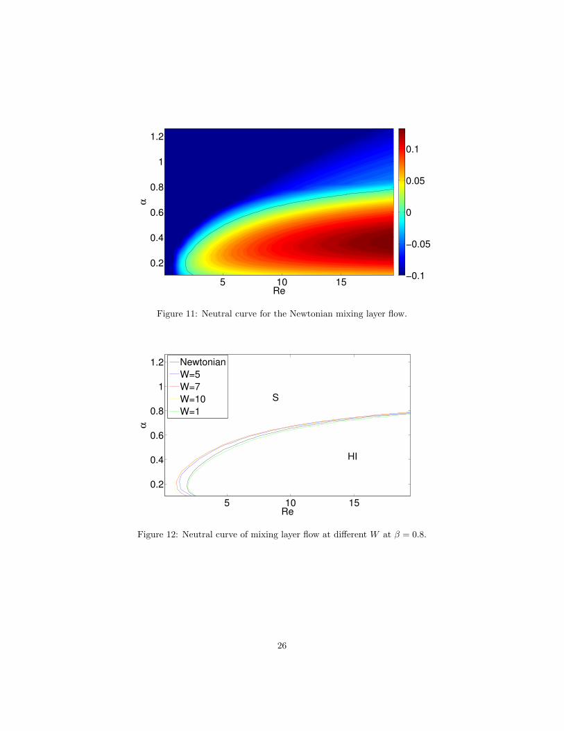
Next we consider a mixing layer whose base flow is u = tanh(y); the neutralcurve for Newtonian fluid is plotted in figure (11). Unlike the jet flow, the mixinglayer does not show a new unstable region at vanishing Re when a strongerelastic effect is present (see figure (12)). Instead, the critical Re first slightlyincreases at W ≈ 1 and then decreases when W increases. In fact, as will beshown in the energy analysis, the instability at largeW will turn to elastic nature(instability due to the destabilizing effect of the increasing polymer normal stress[40]) when E = W/Re & 1. Decreasing β has a destabilizing effect on the flow,as shown in figure (13). The energy analysis will be performed subsequently toreveal the reason.

25

Re

α

5 10 15

0.2

0.4

0.6

0.8

1

1.2

−0.1

−0.05

0

0.05

0.1

Figure 11: Neutral curve for the Newtonian mixing layer flow.

Re

α

5 10 15

0.2

0.4

0.6

0.8

1

1.2 Newtonian

W=5

W=7

W=10

W=1

S

HI

Figure 12: Neutral curve of mixing layer flow at different W at β = 0.8.

26

Re

α

5 10 15

0.2

0.4

0.6

0.8

1

1.2 Newtonian

β=0.8

β=0.6S

HI

Figure 13: Neutral curve of mixing layer flow at different β at W = 7.

Before next section, we give the reason why in the mixing layer flow there isno elastic instability region emerging at vanishing Re while in jet flow this oc-curs. The main argument is that in mixing layer, the shear effect at very low Reonly extends the polymer molecules at the flow interface of different velocitieswhile in the jet, the polymer chains are stretched in the two adjacent layers,interaction between which will probably give rise to instability. To verify thisargument, two new base flows are considered as

u3 = tanh(y)sech2(y) y ∈ (−10, 10) (50)

u4 = −2sech2(y)tanh2(y) + sech4(y) y ∈ (−10, 10) (51)

−10 −5 0 5 10−0.4

−0.2

0

0.2

0.4

y

u

(a)

−1 −0.5 0 0.5 1−0.5

0

0.5

1

1.5

y

du

/dy

(b)

Figure 14: New base flow (a) u3, (b) du3

dy .

27

−10 −5 0 5 10−0.4

−0.2

0

0.2

0.4

0.6

0.8

1

y

u

u4

Jet flow

(a)

−1 −0.5 0 0.5 1−3

−2

−1

0

1

2

3

y

du/d

y

(b)

Figure 15: ew base flow (a) u4 and jet, (b) du4

dy .

The flow u3 consists of three inflectional points and u4 four such points,see figure(14b) and (15b). One can see that in u3 profile there is an interfacebetween flows of two different velocities at the centerline, similar to mixinglayer, however, we expect that disturbance at very low Re will lead this flowto instability because there are adjacent shearing layers besides the interface.This is true since at β = 0.8,W = 20, R = 0.1, α = 0.4, γ = 0, the flowbecomes elastically unstable (imaginary part of least stable eigenvalue ωi =0.003498934598863). On the other hand, u4 is compared to jet flow in figure(15a). Because the adjacent shearing layers are closer in u4 and there are alsosmall adjacent shearing layers at negative velocities, we expect that the growthrate of u4 is larger than jet flow at the same parameters when there is an elasticinstability region in the vanishing Re limit. This is true according to table (3).

Table 3: Disturbance growth rate ωi of u4 and jet at the same parametersFlows Growth ratejet 0.017235583628661u4 0.072818116187888

4.2 Eigenfunction

According to linear stability analysis, eigenfunction of the system can be readilyobtained from the eigenvalue problem (22). The eigenfunction for jet flow atW = 10, β = 0.8, Re = 14.77, α = 0.82, γ = 0 is shown in figure (16). Fromneutral curve (8), we know that this instability is of hydrodynamic nature. Theeigenfunction at W = 10, β = 0.8, Re = 0.01, α = 0.82, γ = 0 is shown infigure (17). In this case, the instability is due to the elasticity of the polymermolecules. One can note that the hydrodynamic jet mode is antisymmetric in u,whereas the elastic mode is symmetric in u. The eigenfunction for mixing layerat W = 10, β = 0.8, Re = 2, α = 0.66 is shown in figure (18). The instability isof elastic nature, thus, the u mode is also symmetric.

28

−10 −5 0 5 100

0.5

1

1.5x 10−4

y

u modev mode

(a)

−10 −5 0 5 100

0.01

0.02

0.03

0.04

y

τ11

τ22

τ12

(b)

Figure 16: (a) Eigenfunction and (b) polymer stress of jet flow at W = 10, β =0.8, Re = 14.77, α = 0.82. It is hydrodynamic instability.

−10 −5 0 5 100

1

x 10−4

y

u modev mode

(a)

−10 −5 0 5 100

0.01

0.02

0.03

y

τ11

τ22

τ12

(b)

Figure 17: (a) Eigenfunction and (b) polymer stress of jet flow at W = 10, β =0.8, Re = 0.01, α = 0.82. It is elastic instability.

−10 −5 0 5 100

1

x 10−4

y

u modev mode

(a)

−10 −5 0 5 100

0.01

0.02

0.03

y

τ11

τ22

τ12

(b)

Figure 18: (a) Eigenfunction and (b) polymer stress of mixing layer flow atW = 10, β = 0.8, Re = 2, α = 0.2. It is elastic instability.

29

4.3 Energy Analysis

The energy analysis can be used to explain instability mechanisms in the flows.In order to make the comparison between different cases meaningful, all theterms in equation (28) are normalized with the integral of the perturbationenergy

∫ΩedV , so we are dealing with the normalized energy density as in

equation (29). Energy analysis is performed with different Re and W , bothof which can provide the quantitative differences between various energy termswith varying elastic effect in the flows.

Table 4: Energy analysis of Newtonian jet flowTerms Re = 4(N) Re=6(N) Re = 10(N) Re = 16(N)V D11 -0.040 -0.036 -0.030 -0.022V D12 -0.131 -0.148 -0.148 -0.131V D21 -0.140 -0.084 -0.042 -0.023V D22 -0.040 -0.036 -0.030 -0.022

V D -0.350 -0.304 -0.249 -0.198P 0.231 0.287 0.332 0.348

Total -0.119 -0.017 0.082 0.150

Table (4) shows the results of Newtonian jet flow with varying Re (The Nbehind Re represents Newtonian flow). Production against mean flow increaseswith Re whereas viscous dissipation decreases leading to instability. This isthe well-known mechanism leading to instability in Newtonian flow. The resultof energy analysis on viscoelastic flow at W = 10, β = 0.8, α = 0.6, γ = 0(Chebyshev modes are 131) and different Re is shown in table (5). PD, asmentioned before, refers to elastic work rate, V D viscous dissipation (alwaysnegative) and P production against the base flow shear. The subscript numbersrepresent different directions.

30

Table 5: Energy analysis of viscoelastic jet flow with varying ReTerms Re = 4 Re = 6 Re = 10 Re = 16PD11 1.041 0.859 0.693 0.182PD12 -0.252 -0.227 -0.211 -0.095PD21 -0.045 -0.034 -0.023 -0.028PD22 -0.034 -0.024 -0.015 -0.019V D11 -0.089 -0.062 -0.038 -0.021V D12 -0.359 -0.299 -0.238 -0.117V D21 -0.055 -0.034 -0.019 -0.015V D22 -0.089 -0.062 -0.038 -0.021

PD 0.711 0.574 0.444 0.040V D -0.591 -0.456 -0.334 -0.174P -0.096 -0.107 -0.119 0.217

Total 0.023 0.011 -0.009 0.0822ωi 0.023 0.011 -0.009 0.082

The prediction is consistent with the result of linear stability analysis, i.e.,time variation of total energy is positive if the flow is unstable while negativeif the flow is stable. Besides, as mentioned before, the value of Re in equation(29) should be exactly equal to two times the imaginary part of least stableeigenvalue. Figure (19) shows this fact, so that we validate our results. Therelative difference between these two values is usually 10−7 at Chebyshev modesbeing 131.

0 5 10 15

0

0.02

0.04

0.06

0.08

0.1

Re

Eigenvalues*2R

e

Figure 19: The least stable eigenvalues and Re at W = 10, β = 0.8, α = 0.6, γ =0.

31

In table (5), the instability at Re = 16 is of hydrodynamic nature, whileat Re = 6 we have elastic instability. Note that in hydrodynamic instabilitythe polymer work rate PD may be positive (in this particular case W = 10, soW/Re ≈ 1, the elastic effect is still significant), but the main destabilizing effectcomes from the production P ; the opposite holds for EI. With increasing Re,the production P increases, viscous dissipation V D decreases and the elasticwork rate PD decreases. Interestingly, it can be seen that production againstthe mean shear is positive in the hydrodynamic instability region (Re = 16)while is negative in the elastic instability region (Re = 6 or 4). It is importantto note that when an instability occurs, disturbance energy is generated onlyby the term PD11, interaction between the fluctuating polymer stress and the

fluctuating flow field, i.e., −∫

Ω1−β2Re (τ11

∂u∗1∂x1

+ τ∗11∂u1

∂x1)dV in the energy equation

(28). Besides, comparing the results of viscoelastic and Newtonian flows, wecan see that with the presence of polymers, the production against base flowshear is reduced. The data are also presented visually in figure (20).

4 6 8 10 12 14 16

−0.4

−0.2

0

0.2

0.4

0.6

Re

Energ

y

PD

VD

P

T

VD(N)

P(N)

T(N)

Figure 20: PD, VD, P and T in viscoelastic and Nowtonian jet flow with varyingRe.

Next we present the energy analysis on jet with varying W at β = 0.8, Re =7, α = 0.6, γ = 0 in table (6). W = 0 is the Newtonian limit. The data isas well visualized in figure (21a). One can see that at small W , the sum ofPD and V D terms remains constant. When W increases to 5, the PD and Pcurves cross over each other, after which PD increases significantly, leading theflow to elastic instability. At the same time, production against mean shear Pdecreases dramatically with W around 5, but when PD reaches a saturation,P as well decreases slowly. Therefore, it is clear that at small W , the flow isstabilized (see black line T ) due to the polymer molecules reducing productionagainst mean shear P , and destabilized at larger W because of the increasing

32

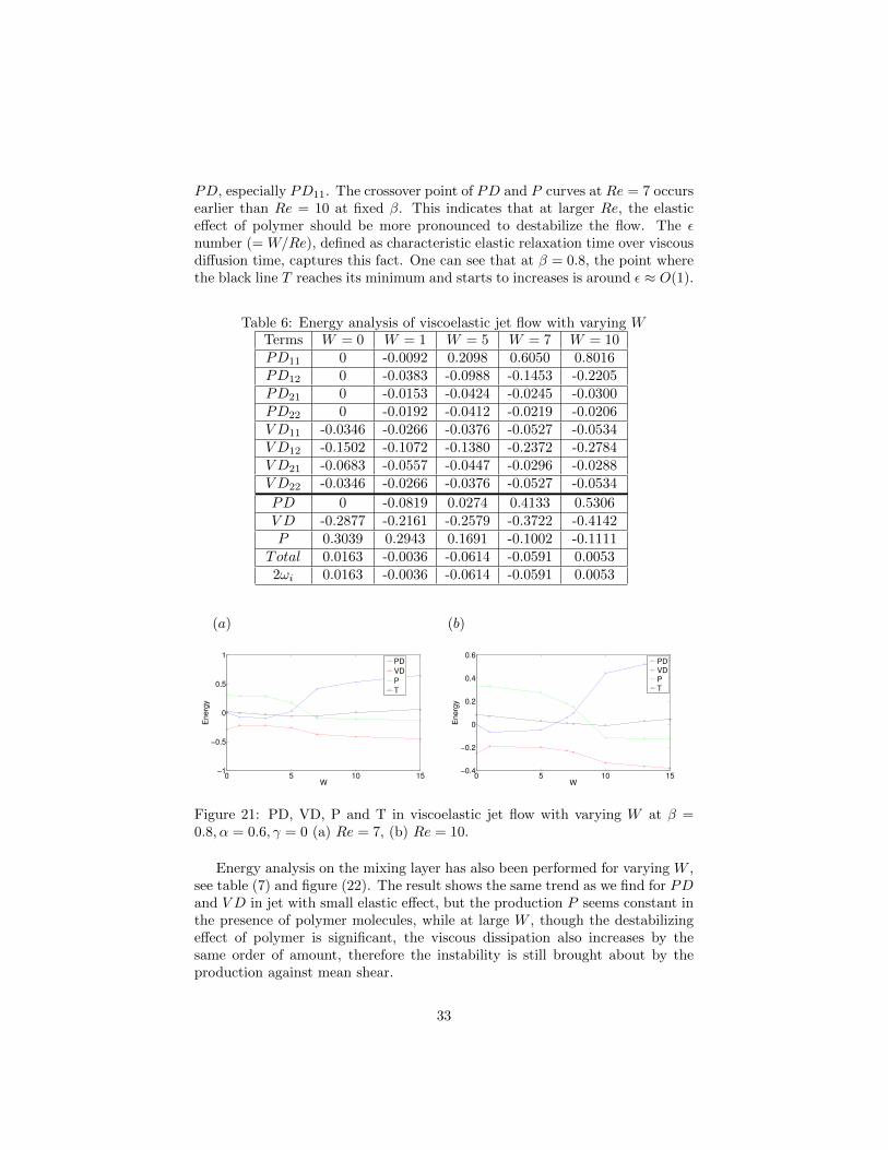
PD, especially PD11. The crossover point of PD and P curves at Re = 7 occursearlier than Re = 10 at fixed β. This indicates that at larger Re, the elasticeffect of polymer should be more pronounced to destabilize the flow. The εnumber (= W/Re), defined as characteristic elastic relaxation time over viscousdiffusion time, captures this fact. One can see that at β = 0.8, the point wherethe black line T reaches its minimum and starts to increases is around ε ≈ O(1).

Table 6: Energy analysis of viscoelastic jet flow with varying WTerms W = 0 W = 1 W = 5 W = 7 W = 10PD11 0 -0.0092 0.2098 0.6050 0.8016PD12 0 -0.0383 -0.0988 -0.1453 -0.2205PD21 0 -0.0153 -0.0424 -0.0245 -0.0300PD22 0 -0.0192 -0.0412 -0.0219 -0.0206V D11 -0.0346 -0.0266 -0.0376 -0.0527 -0.0534V D12 -0.1502 -0.1072 -0.1380 -0.2372 -0.2784V D21 -0.0683 -0.0557 -0.0447 -0.0296 -0.0288V D22 -0.0346 -0.0266 -0.0376 -0.0527 -0.0534

PD 0 -0.0819 0.0274 0.4133 0.5306V D -0.2877 -0.2161 -0.2579 -0.3722 -0.4142P 0.3039 0.2943 0.1691 -0.1002 -0.1111

Total 0.0163 -0.0036 -0.0614 -0.0591 0.00532ωi 0.0163 -0.0036 -0.0614 -0.0591 0.0053

0 5 10 15−1

−0.5

0

0.5

1

W

Energ

y

PD

VD

P

T

(a)

0 5 10 15−0.4

−0.2

0

0.2

0.4

0.6

W

Energ

y

PDVDPT

(b)

Figure 21: PD, VD, P and T in viscoelastic jet flow with varying W at β =0.8, α = 0.6, γ = 0 (a) Re = 7, (b) Re = 10.

Energy analysis on the mixing layer has also been performed for varying W ,see table (7) and figure (22). The result shows the same trend as we find for PDand V D in jet with small elastic effect, but the production P seems constant inthe presence of polymer molecules, while at large W , though the destabilizingeffect of polymer is significant, the viscous dissipation also increases by thesame order of amount, therefore the instability is still brought about by theproduction against mean shear.

33

Table 7: Energy analysis of viscoelastic mixing layer at β = 0.8, Re = 2, α =0.6, γ = 0

Terms W = 0 W = 0.5 W = 1 W = 2 W = 5PD11 0 -0.0087 -0.0075 0.0033 0.1400PD12 0 -0.0249 -0.0272 -0.0302 -0.0683PD21 0 -0.0004 -0.0019 -0.0067 -0.0166PD22 0 -0.0092 -0.0097 -0.0106 -0.0127V D11 -0.0212 -0.0169 -0.0168 -0.0171 -0.0198V D12 -0.1297 -0.0986 -0.0950 -0.0957 -0.1430V D21 -0.0188 -0.0151 -0.0152 -0.0149 -0.0122V D22 -0.0212 -0.0169 -0.0168 -0.0171 -0.0198

PD 0 -0.0431 -0.0464 -0.0442 0.0424V D -0.1910 -0.1474 -0.1438 -0.1448 -0.1950P 0.2084 0.2048 0.2026 0.2040 0.2078

Total 0.0174 0.0143 0.0123 0.0149 0.05542ωi 0.0174 0.0143 0.0123 0.0149 0.0554

0 5 10 15−0.4

−0.2

0

0.2

0.4

W

Energ

y

PD

VD

P

T

Figure 22: PD, VD, P and T in viscoelastic mixing layer with varying W atβ = 0.8, Re = 2, α = 0.6, γ = 0.

To summarize, in the jet flow, but not for mixing layer, polymer stretchingcreates production of disturbance kinetic energy and an instability of elastic na-ture at low Re, whereas mixing layer only stretches the polymer at the interface.At larger Re and small W for both flows, the instability is of hydrodynamic na-ture, caused by production against the mean shear, and polymers have a slightlystabilizing effect at small elastic effect in the jet flow. At larger W in jet, the

34

main destabilizing effect is brought about by the polymer normal stress, leadingto instability, but in mixing layer, the production against mean shear is stillthe main reason leading to instability and the polymer destabilizing effect isdissipated by the viscosity.

35

5 Results of Poiseuille Flow

The viscoelastic Poiseuille flow is investigated and we present here the resultsfor neutral curves, modal energy analysis and non-modal analysis.

5.1 Neutral Curves

Neutral curves in this chapter are plotted in (α,Re) and (W,Re) planes withdifferent viscoelastic parameters. The results generally depict FENE-P modelin 2D, but results for Newtonian and Oldroyd-B fluids in flows at the samepressure gradient will be presented as well . (Note that the Squire’s theorem forFENE-P Poiseuille flow has not been proven.) There are no background colorin the figures indicating stable and unstable regions, but the convention is thaton the left hand side of curve (low Re), the flow is stable and on the right handside unstable.

Re

α

5000 5500 6000 6500 7000 7500 8000 85000.8

0.85

0.9

0.95

1

1.05

1.1

1.15

W=10

W=5

W=1

W=0.5

Newtonian

Figure 23: Neutral curves at β = 0.9, L = 60, γ = 0 with different W .

Figure (23) displays the effect of W at β = 0.9, L = 60, γ = 0. It can be seenthat at larger W , the strong elastic effect results in stabilization for FENE-Pfluids . But interestingly, at small W (around 1), the flow is less stable. Thistrend may be clearer in the following figure (26).

36

5000 5500 6000 6500 7000 7500 8000 85000.8

0.85

0.9

0.95

1

1.05

1.1

1.15

Re

α

β=0.7

β=0.8

β=0.9

Newtonian

(a)

5000 5500 6000 6500 7000 7500 8000 85000.8

0.9

1

1.1

β=0.7

β=0.8

β=0.9

Newtonian

(b)

Figure 24: Neutral curves in (α,Re) space at W = 10, L = 60, γ = 0 withdifferent β (a) for FENE-P, (b) for Oldroyd-B.

Figure (24) shows the effect of viscosity ratio β at W = 10, L = 60, γ = 0 forFENE-P and W = 10, γ = 0 for Oldroyd-B. One can see that with decreasing β(which amounts to increasing polymer molecule concentration), the critical Refor FENE-P fluid decreases, i.e., at this W , stronger elastic effect stabilizes theflow. For Oldroyd-B fluid at W = 10, decreasing β (with β in Newtonian casebeing 1) first stabilizes, then destabilizes the flow. But the effect is smaller thanthe stabilization of FENE-P model once one compares the figures above. Notethat the conclusion is drawn within the range of large β.

2000 4000 6000 8000 10000 12000 140000

5

10

15

Re

W

β=0.5 FENE−P

β=0.7 FENE−P

β=0.9 FENE−P

β=0.5 Oldroyd−B

β=0.7 Oldroyd−B

β=0.9 Oldroyd−B

Figure 25: Neutral curves in (Re,W) plane at L = 60, γ = 0 with different β.

37

−5000 0 5000 10000 150000

5

10

15

(Re−5772)/(1−β)

W

β=0.5 FENE−P

β=0.7 FENE−P

β=0.9 FENE−P

β=0.5 Oldroyd−B

β=0.7 Oldroyd−B

β=0.9 Oldroyd−B

Figure 26: Neutral curves in ((Re-5772)/(1-β),W) plane at L = 60, γ = 0 withdifferent β.

−5000 0 5000 10000 15000 200000

1

2

3

4

(Re−5772)/(1−β)

W*ω

r

β=0.4 FENE−P

β=0.5 FENE−P

β=0.6 FENE−P

β=0.7 FENE−P

β=0.8 FENE−P

β=0.9 FENE−P

Figure 27: Neutral curves in ((Re-5772)/(1-β),W*ωr) plane at L = 60, γ = 0with different β.

Figure (25) and (26) show the relation between W and the critical Re fordifferent β for the two models, FENE-P and Oldroyd-B. Critical Re implies thatthe values of Re are obtained by searching a minimum in the (α,Re) plane for

38

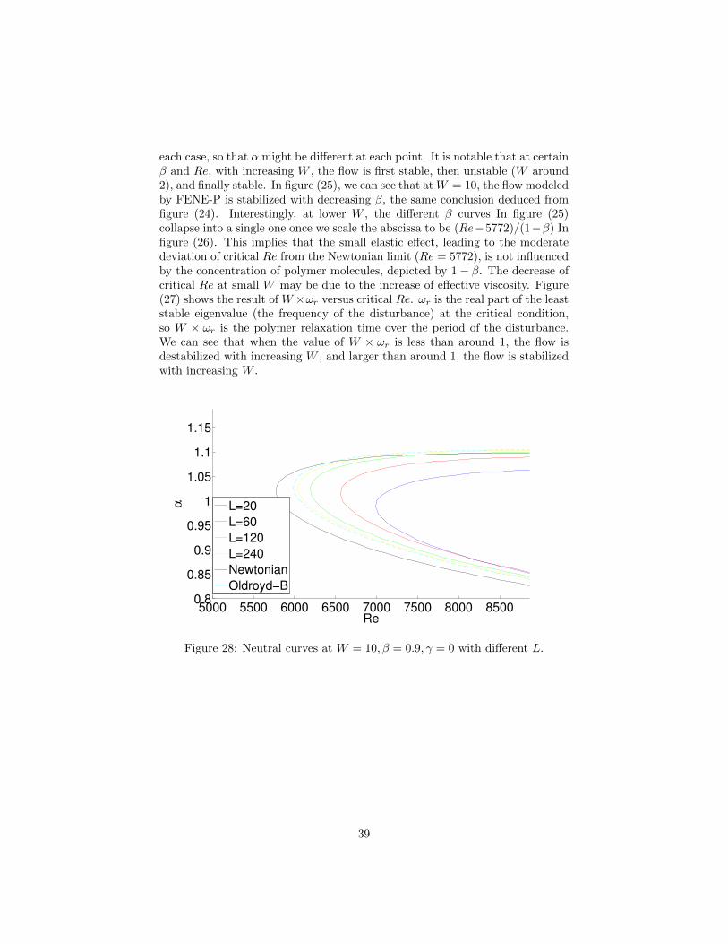
each case, so that α might be different at each point. It is notable that at certainβ and Re, with increasing W , the flow is first stable, then unstable (W around2), and finally stable. In figure (25), we can see that atW = 10, the flow modeledby FENE-P is stabilized with decreasing β, the same conclusion deduced fromfigure (24). Interestingly, at lower W , the different β curves In figure (25)collapse into a single one once we scale the abscissa to be (Re−5772)/(1−β) Infigure (26). This implies that the small elastic effect, leading to the moderatedeviation of critical Re from the Newtonian limit (Re = 5772), is not influencedby the concentration of polymer molecules, depicted by 1− β. The decrease ofcritical Re at small W may be due to the increase of effective viscosity. Figure(27) shows the result of W×ωr versus critical Re. ωr is the real part of the leaststable eigenvalue (the frequency of the disturbance) at the critical condition,so W × ωr is the polymer relaxation time over the period of the disturbance.We can see that when the value of W × ωr is less than around 1, the flow isdestabilized with increasing W , and larger than around 1, the flow is stabilizedwith increasing W .

5000 5500 6000 6500 7000 7500 8000 85000.8

0.85

0.9

0.95

1

1.05

1.1

1.15

Re

α

L=20

L=60

L=120

L=240

Newtonian

Oldroyd−B

Figure 28: Neutral curves at W = 10, β = 0.9, γ = 0 with different L.

39

5000 5500 6000 6500 7000 75000

5

10

15

Re

W

L=60

L=120

L=240

Oldroyd−B

Figure 29: Neutral curves at β = 0.9, γ = 0 with different L.

The effect of L, the maximum extension of polymer molecule, is presentednext. The result is shown in figure (28) where we choose W = 10, β = 0.9.Oldroyd-B model is simply the limit of FENE-P model when L goes to infinity,therefore, the result of the Oldroyd-B model is shown as a limiting case of aseries of FENE-P model with increasing L. The shorter L, the stronger elasticeffect the polymer molecules can display, though the stronger normal stressgradient is found in longer L case. As seen from the figure (28), smaller L showsstabilization of the flow, which in some extent is consistent with the previousresults for W = 10 case (stronger elasticity stabilizes the flow). As will be shownin the energy analysis, the reason of smaller L resulting in more stable flow isthat at small L, the production against the mean shear P is inhibited. Theeffect of L is also presented in the (W,Re) plane in figure (29), where Re is thecritical Re. But unlike for β in figure (26), at all theW investigated, increasing Ldestabilizes the flow. This suggests that L, elasticity, always stabilizes the flow,while polymer viscosity simply enhances the effect of the viscoelastic additives.

Since there is no Squire’s theorem for viscoelastic flow of non-linear consti-tute model (e.g. FENE-P in our study), we investigated (α, γ) plane as shownin figure (30). The most unstable region is around α = 1, γ = 0. At γ = 0, if γincreases a little, the least stable ωi will decrease compared to γ = 0 case (notclear from the figure), meaning that the flow in 2D is more unstable in thesecases.

40

γ

α

0.5 1 1.5

0.5

1

1.5

−12

−10

−8

−6

−4

−2

0x 10

−3

Figure 30: Neutral curve in (α, γ) plane at β = 0.9,W = 5, L = 60, Re = 6000.

5.2 Energy Analysis

The energy analysis of FENE-P Poiseuille flow is presented in this section. Aswe linearize the equation, the expressions for perturbed polymer stress τij aredifferent in the two constitutive models due to their different definitions. InOldroyd-B model, τij is simply

cijW , where the perturbed conformation tensor

could be readily extracted from the resultant eigenfunction. However, in FENE-

P model, τij isf ′Cij+fcij

W , where f and f ′ are defined previously in equations

Table 8: Energy analysis of viscoelastic Poiseuille flowTerms W = 0 W = 0.5 W = 2.5 W = 6PD11 0 -1.378E-04 -2.817E-04 3.416E-04PD12 0 -1.355E-03 -1.226E-03 -1.641E-03PD21 0 1.537E-05 2.430E-06 -2.601E-05PD22 0 -5.426E-05 -6.130E-05 -6.688E-05V D11 -2.673E-04 -2.406E-04 -2.406E-04 -2.408E-04V D12 -1.429E-02 -1.288E-02 -1.300E-02 -1.317E-02V D21 -1.043E-04 -9.385E-05 -9.380E-05 -9.363E-05V D22 -2.673E-04 -2.406E-04 -2.406E-04 -2.408E-04

PD 0 -1.531E-03 -1.567E-03 -1.392E-03V D -1.493E-02 -1.345E-02 -1.358E-02 -1.375E-02P 1.432E-02 1.478E-02 1.561E-02 1.400E-02

Total -6.031E-04 -2.067E-04 4.657E-04 -1.137E-032ωi -6.031E-04 -2.067E-04 4.657E-04 -1.137E-03

41

(5) and (18).Table (8) shows the results of energy analysis at β = 0.9, Re = 5600, L =

60, α = 1.02, γ = 0. W = 0 case amounts to Newtonian flow. The results haveall been normalized by the integral of perturbed energy. The total energy is thesum of PD, V D and P , while the value of 2ωi is directly read from the resultanteigenvalue. According to equation (29), these two values should be exactly thesame, and this is validated in the table. The result is better presented in plots.Data in figure (31) to (33) pertain to cases with β=0.9, 0.7 and 0.5, respectively.(Note that Re are different in the three cases.) One can see from these figuresthat the total dissipation is almost constant changing W . When polymer workrate decreases, the viscous dissipation increases and vise versa. At low W ,the flow instability is determined by the increase of production. On the otherhand, at large W , the flow is stabilized because of less production. This trendis more obvious for stronger elastic effect, lower β. Note that in the case ofβ = 0.5,W = 10, the production could be negative and the polymer work ratepositive.

0 2 4 6 8 10−0.02

−0.01

0

0.01

0.02

W

En

erg

y

PDVDPTotal

Figure 31: Normalized energy results in a function of W at β = 0.9, Re =5600, L = 60, α = 1.02, γ = 0.

42

0 2 4 6 8 10−0.02

−0.01

0

0.01

0.02

W

Energ

y

PDVDPTotal

Figure 32: Normalized energy results in a function of W at β = 0.7, Re =5300, L = 60, α = 1.02, γ = 0.

0 2 4 6 8 10−0.02

−0.01

0

0.01

0.02

W

Ene

rgy

PDVDPTotal

Figure 33: Normalized energy results in a function of W at β = 0.5, Re =5000, L = 60, α = 1.02, γ = 0.

Briefly, the energy analysis of different L is presented in table (9) at β =0.9,W = 6, Re = 5600, α = 1.02, γ = 0. It is clear that at small L the productionagainst mean shear P is decreased while PD and V D are close. Therefore longerL leads to more unstable flow as shown in the figure (29).

43

Table 9: Energy analysis for different LTerms(10−4) L = 60 L = 120 L = 500

PD11 3.416 3.621 3.745PD12 -16.412 -16.978 -17.202PD21 -0.260 -0.286 -0.296PD22 -0.669 -0.689 -0.696V D11 -2.408 -2.408 -2.408V D12 -131.730 -131.746 -131.779V D21 -0.936 -0.937 -0.937V D22 -2.408 -2.408 -2.408

PD -13.925 -14.333 -14.449V D -137.482 -137.498 -137.530P 140.032 147.161 149.969

Total -11.375 -4.670 -2.0102ωi -11.375 -4.670 -2.010

The phase difference between the eigenfunctions u (phase is θ1) and v (phaseis θ2) is shown in figure (34). It is the phase difference which gives rise toproduction against the mean shear if it is not 90, in which case production willbe 0. The production distribution along wall-normal direction is presented infigure (35). We can see from these two figures that the production is mainlygenerated in a region near the wall, the critical layer, whereas it is almost zeroin the bulk of the flow domain. Varying W will decrease the negative value ofproduction in the critical layer more than increase its positive value, so that thetotal production is less.

−0.05 0 0.05 0.1 0.15 0.2 0.25 0.3−1

−0.5

0

0.5

1

cos(θ1−θ2)

y

W=10

W=6

W=2.5

W=0.5

Figure 34: Cosine of the phase difference between u and v along the wall-normaldirection.

44

−0.04 −0.02 0 0.02 0.04 0.06 0.08 0.1−1

−0.5

0

0.5

1

Energy

y

W=10

W=6

W=2.5

W=0.5

Figure 35: Distribution of production against mean shear along the wall-normaldirection.

To sum up, we observe that production increases at W × ωr . 1, peaksaround W × ωr ≈ 1 and then decreases fast. Dissipation is almost constantfor W × ωr . 1, equal to the Newtonian case for the same total viscosity sincein this region polymers are almost unelastic. The destabilization can thereforebe explained by increasing effective viscosity and increasing viscous production(|uv|cos(θ1 − θ2)). Stabilization occurs at W × ωr & 1. In this case, stretchedpolymers decrease dissipation, but at the same time decrease production againstmean shear as well, the latter effect being dominant.

5.3 Transient Growth

The non-modal linear stability analysis (which accounts for the flow stabilityin a short time) on non-Newtonian Poiseuille flow has not been explored asextensively as modal analysis until recently. In this section we aim to investigatethe transient growth of disturbance in the Poiseuille flow modeled by FENE-Pas well as Oldroyd-B and Newtonian for comparison. As mentioned in Chapter2, only fluid disturbance is considered at the moment and the response also onlyconcerns the fluid.

With respect to wavenumbers, we focus primarily on γ = 2 for spanwisedirection. Transient growth at different γ and L = 60, β = 0.9,W = 10, Re =6000, α = 0 has been calculated as shown in figure (36) together with Newtonianflow, where one can see that γ = 2 gives rise to the maximum of Gmax. Forstreamwise wavenumber, α = 0 is of particular interest because this combination(α = 0, γ = 2) will give the maximum ofGmax (Schmid & Henningson 2001 [41]).In non-modal analysis for Newtonian flow, vanishing streamwise wavenumbercorresponds to the streaks structure which is the optimal mechanism leadingthe flow to transition. In order to consider different streamwise wavenumbers,

45

results of other α value will also be presented.

0.5 1 1.5 2 2.5 3 3.5 42000

3000

4000

5000

6000

7000

8000

γ

Gm

ax

Viscoelastic flow

Newtonian flow

Figure 36: Gmax changes as γ increases for viscoelastic flow at L = 60, β =0.9, Re = 6000,W = 10, α = 0 and Newtonian flow.

In figure (37) and (38) transient growth with different L is shown at α = 0,α = 1.02 and α = 2. Also Gmax changing with L is displayed in figure (38b),in which one can see that at larger L the normalized transient growth (withrespect to the data of respective Newtonian flow) asymptotically approach afixed value while the transient growth at L = 60 increases only 3% or even less. Selected data are listed in table (10). Therefore, we could say the effect of Lon transient growth is negligible.

0 200 400 600 800 10000

500

1000

1500

2000

2500

3000

3500

Time

G(t

)

L=60L=120Oldroyd−BNewtonian

L

(a)

0 20 40 60 80 1000

100

200

300

400

Time

G(t

)

L=60L=120Oldroyd−BNewtonian

L

(b)

Figure 37: Transient growth changes with L at β = 0.9,W = 10, Re = 4000, γ =2 (a) α = 0, (b) α = 1.02

46

0 20 40 60 80 1000

50

100

150

Time

G(t

)

L=60L=120Oldroyd−BNewtonianL

(a)

0 100 200 300 400 5000.92

0.94

0.96

0.98

1

1.02

1.04

1.06

L

Gm

ax

α=0

α=1.02

α=2

(b)

Figure 38: Transient growth changes with L at β = 0.9,W = 10, Re = 4000, γ =2 (a) α = 2, (b) normalized Gmax with respect to the value of Newtonian flow.

Table 10: Selected data in figure (38b).L = 60 L = 120 L = 240 L = 500

α = 0 3263.52 3201.03 3180.81 3175.10α = 1.02 391.24 387.60 386.68 386.46α = 2 127.6 126.32 125.98 125.89

Figure (39) to (41) shows the influence of β. It is clear that at α = 0, smallβ yields larger transient growth while at α = 1.02 and α = 2 the oppositehappens. The Gmax is also shown in these figures with a logarithm scale, whereone observes an almost linear dependence of the maximum transient growth onβ.

0 200 400 600 800 10000

2000

4000

6000

8000

10000

Time

G(t

)

β=0.9

β=0.7

β=0.5

Newtonian

β

(a)

10−1

100

102

103

104

1−β

Gm

ax−

GN

DataG

max−G

N=2500*(1−β)

(b)

Figure 39: Transient growth versus β at L = 60,W = 10, Re = 6000, γ = 2 (a)α = 0, (b) Gmax −GN versus 1− β in a logarithm scale.

47

0 20 40 60 80 1000

200

400

600

800

Time

G(t

)

β=0.9

β=0.7

β=0.5

Newtonian

β

(a)

10−1

100

101.2

101.4

101.6

101.8

1−β

GN

−G

ma

x

DataG

N−G

max=150*(1−β)

(b)

Figure 40: Transient growth versus β at L = 60,W = 10, Re = 6000, γ = 2 (a)α = 1.02, (b) GN −Gmax versus 1− β in a logarithm scale.

0 20 40 60 80 1000

50

100

150

200

Time

G(t

)

β=0.9

β=0.7

β=0.5

Newtonian

β

(a)

10−1

100

100

101

102

1−β

GN

−G

ma

x

DataG

N−G

max=80*(1−β)

(b)

Figure 41: Transient growth versus β at L = 60,W = 10, Re = 6000, γ = 2 (a)α = 2, (b) GN −Gmax versus 1− β in a logarithm scale.

The dependence of transient growth on Re has also been investigated. Notethat the Re in polymer solution is based on the total viscosity, which thereforedepicts the property for the whole flow. In Newtonian non-modal analysis,appropriate scaling will lead to the conclusion that the maximum transientgrowth is proportional to Re2 (Schmid & Henningson 2001 [41]). Figure (42)shows this fact in both viscoelastic and Newtonian flow in a logarithm scaleat α = 0, where one can see that the Gmax is larger in the polymer solution.At α = 1.02 figure (43) shows that Gmax now is linearly proportional to Re.In this streamwise wavenumber, the Gmax of Newtonian flow is slightly larger.Additionally, the time when Gmax happens (Tmax) is a linear function of Rein the Newtonian flow; figure (44) indicates that with the polymer Tmax is stilllinearly dependent on Re and is almost the same time compared to Newtonianflow.

48

103

104

102

103

104

105

Re

Gm

ax

Viscoelastic flow

Newtonian flow

Gmax

=Re2 line

Figure 42: Gmax changes as Re increases at β = 0.9, L = 60,W = 10, α =0, γ = 2 in a logarithm scale.

103

104

101

102

103

104

105

Re

Gm

ax

Viscoelastic flow

Newtonian flow

Gmax

=Re line

Figure 43: Gmax changes as Re increases at β = 0.9, L = 60,W = 10, α =1.02, γ = 2 in a logarithm scale.

49

103

104

102

104

Re

Tm

ax

Viscoelastic flow

Newtonian flow

Tmax

=Re line

Figure 44: Tmax changes as Re increases at β = 0.9, L = 60,W = 10, α = 0, γ =2 in a logarithm scale.

Figure (45) shows how the elastic effect influences the transient growth atL = 60, β = 0.9, Re = 4000, γ = 2 in FENE-P model with different streamwisewavenumber. The data are normalized according to the Newtonian value (W =0) at each α. Part of data are listed in table (11) to compare between differentα. As the figure shows, at small α with increasing W , the Gmax increasesmonotonically, while at larger α, the Gmax slightly increases before W ≈ 1where the elastic effect of polymer molecules is still weak, but decreases whenW is larger than around 1. W is the ratio between the polymer characteristicrelaxation time λ and the flow characteristic time L/U . When λ is small, thepolymer molecules react very fast to the wave propagating in the flow, therefore,they tend to flow along with the surrounding flows without manifesting theirelasticity. On the other hand, when λ is large, the polymer molecules have morepotential of elasticity. From a point of view of energy, the flow perturbationenergy at large W will be absorbed by the polymer (stored as elastic energy),leading to a more stable flow. For α = 0, work by Jovanovic [26][27] has shownthat in the strong elastic flow, the maximum transient growth is scaled as W 2

with respect to the streamwise invariant stochastic disturbance. In our result,once the data is presented in (Gmax,W/Tmax) plane, we found that in theinertia-dominating flow the relation between Gmax and W/Tmax at larger αcollapses to a single line, see figure (46).

50

Table 11: Selected data in figure (45).W = 0 W = 5 W = 10 W = 15

α = 0 3132.03 3183.18 3263.52 3345.28α = 1.02 405.28 401.86 391.24 384.31α = 2 136.70 133.32 127.66 123.65α = 3 54.18 52.01 49.05 46.89

0 5 10 150.85

0.9

0.95

1

1.05

1.1

W

Gm

ax

α=0

α=0.05

α=0.1

α=0.5

α=1.02

α=2

α=3

Figure 45: Transient growth changes as W increases at L = 60, β = 0.9, Re =4000, γ = 2 for different α.

51

0 0.5 1 1.5 2 2.50.8

0.85

0.9

0.95

1

1.05

W/Tmax

Gm

ax

α=0.5

α=1.02

α=2

α=3

α=4

Figure 46: Transient growth versus W/Tmax at L = 60, β = 0.9, Re = 4000, γ =2 for different α.

Next, the results of optimal initial condition and response are presented infigure (47) and (48) at L = 60, β = 0.9,W = 10, Re = 6000, α = 0, γ = 2, whichindicates that the lift-up mechanism still functions in viscoelastic flows. Theoptimal initial condition includes counter-rotating streamwise vortices locatedalong the spanwise direction, while the final response consists only the stream-wise fluctuation velocity and two streaks along the wall-normal direction. For2D case α = 2, γ = 0, the optimal initial condition is the fluctuation flow againstthe mean shear, and the response to it evolves to mean shear direction, whichindicates that the Orr mechanism functions in such flow.

0 0.5 1 1.5 2 2.5−1

−0.5

0

0.5

1

z

y

uin

vin

win

(a)

−2 −1 0 1 2−1

−0.5

0

0.5

1

z

y

(b)

Figure 47: Optimal initial condition at L = 60, β = 0.9,W = 10, Re = 6000, α =0, γ = 2.

52

0 50 100 150 200 250 300−1

−0.5

0

0.5

1

z

y

ure

vre

wre

(a)

z

y

−3 −2 −1 0 1 2 3

−0.5

0

0.5

−200

−100

0

100

200

(b)

Figure 48: Response at L = 60, β = 0.9,W = 10, Re = 6000, α = 0, γ = 2.

0 1 2 3 4−1

−0.5

0

0.5

1

x

y

uin

vin

win

(a)

−2 −1 0 1 2−1

−0.5

0

0.5

1

x

y

(b)

Figure 49: Optimal initial condition at L = 60, β = 0.9,W = 10, Re = 6000, α =2, γ = 0.

0 2 4 6 8 10 12 14−1

−0.5

0

0.5

1

x

y

ure

vre

wre

(a)

−2 −1 0 1 2−1

−0.5

0

0.5

1

x

y

(b)

Figure 50: Optimal initial condition at L = 60, β = 0.9,W = 10, Re = 6000, α =2, γ = 0.

Finally, we present the result of time variation of energy amplification. Theenergy density displayed below is considered in the physical space, therefore

53

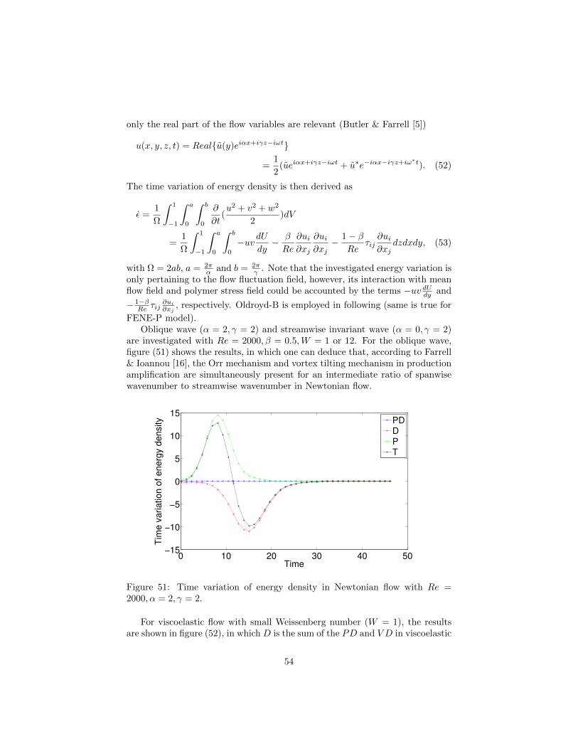
only the real part of the flow variables are relevant (Butler & Farrell [5])

u(x, y, z, t) = Realu(y)eiαx+iγz−iωt

=1

2(ueiαx+iγz−iωt + u∗e−iαx−iγz+iω

∗t). (52)

The time variation of energy density is then derived as

ε =1

Ω

∫ 1

−1

∫ a

0

∫ b

0

∂

∂t(u2 + v2 + w2

2)dV

=1

Ω

∫ 1

−1

∫ a

0

∫ b

0

−uvdUdy− β

Re

∂ui∂xj

∂ui∂xj− 1− β

Reτij

∂ui∂xj

dzdxdy, (53)

with Ω = 2ab, a = 2πα and b = 2π

γ . Note that the investigated energy variation isonly pertaining to the flow fluctuation field, however, its interaction with meanflow field and polymer stress field could be accounted by the terms −uv dUdy and

− 1−βRe τij

∂ui

∂xj, respectively. Oldroyd-B is employed in following (same is true for

FENE-P model).Oblique wave (α = 2, γ = 2) and streamwise invariant wave (α = 0, γ = 2)

are investigated with Re = 2000, β = 0.5,W = 1 or 12. For the oblique wave,figure (51) shows the results, in which one can deduce that, according to Farrell& Ioannou [16], the Orr mechanism and vortex tilting mechanism in productionamplification are simultaneously present for an intermediate ratio of spanwisewavenumber to streamwise wavenumber in Newtonian flow.

0 10 20 30 40 50−15

−10

−5

0

5

10

15

Time

Tim

e v

ariation o

f energ

y d

ensity

PDDPT

Figure 51: Time variation of energy density in Newtonian flow with Re =2000, α = 2, γ = 2.

For viscoelastic flow with small Weissenberg number (W = 1), the resultsare shown in figure (52), in which D is the sum of the PD and V D in viscoelastic

54

flow and V D(N) is the viscous dissipation in Newtonian flow (the PD term isconstantly 0). One can see that D is close to V D(N) and the production termsin the two flows are also close to each other, indicating that at small W , thepolymer molecules behave like the fluid and the elastic effect is negligible. How-ever, with increasing W , the elastic effect starts to work and the result in figure(53) shows that the polymer initially extracts energy from the perturbation fieldand then returns the energy back with the viscous dissipation increasing to al-most the same amount of polymer work rate. In addition, the initial productionin figure (53) is reduced compared to its Newtonian counterpart. Overall, thisdecreased production against mean shear explains the observed reduction intransient growth. The mechanism seems similar to that observed for TollmienSchlichting wave.

0 10 20 30 40 50−15

−10

−5

0

5

10

15

Time

Tim

e v

ariation o

f energ

y d

ensity

PDDPTDVD(N)

Figure 52: Time variation of energy density in viscoelastic flow with Re =2000, β = 0.5,W = 1, α = 2, γ = 2.

55

0 10 20 30 40 50−6

−4

−2

0

2

4

6

8

Time

Tim

e v

ariation o

f energ

y d

ensity

PDDPT

Figure 53: Time variation of energy density in viscoelastic flow with Re =2000, β = 0.5,W = 12, α = 2, γ = 2.

For streamwise invariant wave, the Newtonian result is shown in figure (54),where it shows significant amplification of initial disturbance. The result ofviscoelastic flow at W = 1, Re = 2000, β = 0.5, α = 0, γ = 2 in figure (55)is again similar to the Newtonian flow if we compare the sum of PD and V D(D) in non-Newtonian flow with the V D in Newtonian (productions are alsoclose). The W = 12, Re = 2000, β = 0.5, α = 0, γ = 2 is displayed in figure(56) with Newtonian case as a comparison. One can see that the productionincreases with high W , which indicates that the vortex tilting mechanism isenhanced. The total energy amplification seems to increases since large timevariation is achieved in the viscoelastic flow. This is consistent with what wefound previously in figure (45).

56

0 100 200 300 400 500 600 700−15

−10

−5

0

5

10

15

Time

Tim

e v

ariation o

f energ

y d

ensity

PDVDPT

Figure 54: Time variation of energy density in Newtonian flow with Re =2000, α = 0, γ = 2.

0 100 200 300 400 500 600 700−15

−10

−5

0

5

10

15

Time

Tim

e v

ariation o

f energ

y d

ensity

PD

VD

P

T

D

VD(N)

Figure 55: Time variation of energy density in viscoelastic flow with Re =2000, β = 0.5,W = 1, α = 0, γ = 2. (Red line and blue line are overlapping eachother.)

57

0 200 400 600 800−20

−10

0

10

20

Time

Tim

e v

ariation o

f energ

y d

ensity

VD (N)

P (N)

T (N)

T (W=12)

P (W=12)

D (W=12)

Figure 56: Time variation of energy density in viscoelastic flow with Re =2000, β = 0.5,W = 12, α = 0, γ = 2.

58

6 Conclusion

In this work, the linear stability analysis has been applied to investigate jet,mixing layer and Poisuille flow.

The result of modal stability analysis on polymeric jet indicates that elasticeffect will not only affect the hydrodynamic instability by increasing its criticalRe but also lead to emergence of a new instability mechanism, elastic instability,at small Re. Energy analysis is performed and it is found that the polymerwork rate created by the polymer stretching will increase the kinetic energyof disturbance at small Re while with increasing Re, this part of elastic energydecreases, replaced by the production against mean shear, which finally give riseto hydrodynamic instability at larger Re. Changing W reveals similar trend: atsmall elastic effect, the instability is mainly due to the production against meanshear while at larger W , polymer normal stress destabilizes the flow leading toinstability.

For viscoelastic mixing layer, no instability have been found at vanishing Rebecause the polymer chains are only extended and balanced by the viscous forceat the interface without destabilizing the flow. The instability is brought aboutby the production against mean shear whenever an instability takes place, andthe increasing polymer work rate PD is counteracted by the increasing viscousdissipation.

The results of modal linear stability analysis on viscoelastic Poiseuille flowshow that for fixed other parameters, the flow will first be destabilized at smallW and then become more stable at larger W . The reason behind it seemsto be that at W × ωr . 1 the polymer molecules are almost unelastic, givingrise to increased effective viscosity (Re based on the total viscosity is there-fore reduced). A scaling law has been identified at small W when the datais presented in ((Re − 5772)/(1 − β),W ) plane, which clearly verifies that thepolymer molecules at small W has no significant potential of elasticity. On theother hand at larger W , the elasticity indeed starts to function and it decreasesthe production against the mean shear as shown in the energy analysis.

The results of non-modal linear stability analysis show that for fixed γ,the transient growth of small α increases monotonically whenever W increases,whereas at larger α, Gmax increases slightly at small W less than around 1 anddecreases with increasing W and is found to obey a simple linear scaling whenthe data is presented with W/Tmax, where Tmax is the time for maximum Gmax.The analysis of time variation for energy density performed then reveals that thereason why the transient growth optimized by streamwise invariant disturbance(vanishing α) increases is simply that production against mean shear increasesat the very beginning. Similarly, the decreased production against mean shearfor large α at the beginning also accounts for the decreasing Gmax at larger Wthat we have found in figure (45). For small W , the result of time variationof energy density confirms that the polymer molecules behave like nothing butsurrounding fluid, a fact deduced from the results that the sum of PD and V Dis equal to V D in Newtonian flow with almost same production against meanshear in the two cases. Besides, similar to what has been found in the Newtonian

59

flow, the transient growth optimized by streamwise invariant disturbance inthe inertia-dominating flow is also proportional to Re2 and the time for Gmaxincreases linearly with Re.

60

A Appendix Analytical solution for PoiseuilleFENE-P base flow

From the conformation tensor evolution equation (6) for FENE-P (the subscriptp in the stress tensor is omitted.), we know that (Cruz, Pinho & Oliveira 2005[10])

i = 2, j = 3 : 0 = τ23 =⇒ C23 = 0,

i = 1, j = 3 : −C23u′ = −τ13 =⇒ C13 = 0,

i = 2, j = 2 : 0 = −τ22 =⇒ C22 = 1/f, (54)

i = 3, j = 3 : 0 = −τ33 =⇒ C33 = 1/f, (55)

i = 1, j = 1 : −2C12u′ = −τ11, (56)

i = 1, j = 2 : −2C22u′ = −τ12. (57)

We also have C12

C22= Wτ12 from the definition of the polymer stress, therefore

combining it with equation (56) and (57) yields

τ11 = 2Wτ212. (58)

From the nondimensionalized flow governing equation (11), we have

0 = −dpdx

+β

Re

∂2u

∂y∂y+

1− βRe

∂τ12

∂y, (59)

which once integrated from 0 to y along the wall-normal direction yields

0 = −dpdx

(y − 0) +β

Re(∂u

∂y− ∂u

∂y

∣∣y=0

) +1− βRe

(τ12 − τ12|y=0). (60)

Due to symmetry, the spatial variation of the quantities at y = 0 is 0, so theabove equation simplifies to

∂u

∂y=Re

β

dp

dxy − 1− β

Reτ12. (61)

On the other hand, from equations (54) and (55) we have C22 = C33 = 1/f =

1− Ckk

L2 , which after simple manipulation with equation (57) is equivalent to

C22 =L2

3 + 2W 2τ212 + L2

. (62)

61

Finally, combining equations (57), (61) and (62), we have

τ312 +

L2

2W 2(1 +

3

L2+

1− ββ

)τ12 −L2

2

dp

dx

Re

β

1

W 2y = 0. (63)

Once τ12 (so is τ11) has been obtained, Ckk is given by

Ckk =Wτ11 + 3

L2 +Wτ11 + 3L2. (64)

Then the components of conformation tensor can be derived by

Cij = (Wτij + δij)(1−CkkL2

). (65)

If the Newtonian Poiseuille base flow is u(y) = 1− y2, the modified base flow inFENE-P model is obtained by substituting τ12 into the Navier-Stokes equation(11) and integrating along y direction

u(y) = −Re2β

dp

dx(1− y2)− 1− β

β

3

8C(F+G−

∣∣y−1

+ F−G+

∣∣y−1

), (66)

where

F+ = (Cy +√C2y2 +A3)

13 , F− = (Cy −

√C2y2 +A3)

13 , (67)

G+ = 3Cy +√C2y2 +A3, G− = 3Cy −

√C2y2 +A3, (68)

and

A =L2

6W 2(1 +

3

L2+

1− ββ

), C =L2

4

dp

dx

Re

β

1

W 2. (69)

62

B Appendix Matrices in eigenvalue problem

For Oldryod-B model, matrix A is

(A11 00 I

). A11 comes from the O-S and Sq

equations and it is (∆ 00 I

). (70)

∆ is D2 − k2 and unitary matrix I here has dimension (6N + 12)× (6N + 12).D is the derivative with respect to normal direction and k2 is α2 + γ2.

Matrix B is

(B11 B12

B21 B22

). B11 also originates from the O-S and Sq equations

and it reads (βRe∆2 − iαU∆ + iαU ′′ 0

−iβU ′ βRe∆− iαU

). (71)

B12 is from the interaction between the velocity fluctuation and the stress fluc-tuation in the flow governing equation and it reads(

α2D −k2D γ2D −iα(D2 + k2) 2αγD −iγ(D2 + k2)−αγ 0 αγ iγD α2 − γ2 −iγD

). (72)

B21 is from the stress governing equation and it reads

1

k2

2(−α2C11D + iαC12D2)− k2DC11 2(αγC11 − iγC12D)

2k2(iαC12 + C22D) 0

−2γ2C33D −2αγC33

k2(iαC11 + C12D)− k2DC12

+iαC22D2 − α2C12D αγC12 − iγC22D

−αγC11D + iγC12D2 − αγC33D −α2C11 + iαC12D + γ2C33

iγC22D2 − αγC12D + ik2γC33 −α2C12 + iαC22D

(73)

Terms such as DC11 mean dC11/dy. B22 isK 2U ′

KK

U ′ KK U ′

K

(74)

The empty means zero block. U ′ here represents first derivative of base flow Ualong the normal direction. K equals to −iαU − 1/W .

63

For FENE-P model, the A matrix, B11 and B21 blocks in B matrix arethe same as above because these matrices (blocks) are pertaining to the flowproperties terms in the equations, therefore remain unaltered with differentpolymer constitutive models. The difference lies in B12 and B22 blocks, whichaccount for the polymer properties.

For B12 block, we write it as

B12 =

(vc11 vc22 vc33 vc12 vc13 vc23

ηc11 ηc22 ηc33 ηc12 ηc13 ηc23

). (75)

These coupling terms are between the flow variables and the conformation ten-sors. Before presenting the explicit expression for these coupling terms, thenotation used are present

C ′11 =dC11

dy, C ′22 =

dC22

dy, C ′33 =

dC33

dy(76)

C ′′11 =d2C11

dy2, C ′′22 =

d2C22

dy2, C.′33 =

d2C33

dy2(77)

f ′1 =∂f

∂C11

∣∣∣B

= f ′2 =∂f

∂C22

∣∣∣B

= f ′3 =∂f

∂C33

∣∣∣B

=L2

(L2 − Ckk)2(78)

f ′′1y =∂2f

∂C11∂y= f ′′2y =

∂2f

∂C22∂y= f ′′3y =

∂2f

∂C33∂y=

2L2

(L2 − Ckk)3(C ′11 + C ′22 + C ′33)

(79)

f ′′′1yy =∂3f

∂C11∂y2= f ′′′2yy =

∂3f

∂C22∂y2= f ′′′3yy =

∂3f

∂C33∂y2=

6L2

(L2 − Ckk)4(C ′211 + C ′222 + C ′233) +

2L2

(L2 − Ckk)3(C ′′11 + C ′′22 + C ′′33) (80)

Note that the following expressions could certainly be further simplified sincesome of the terms are equal (such as f ′1 and f ′2), but since the complexity of thederivation originates mainly from the chain rule when taking derivatives, it isbeneficial to keep them not simplified in that such a form is a nature outcomeof the derivative chain rule, so that will reduce the mistake during derivation toa minimum. (Symbol ∗ denotes plain multiplying operation.)

64

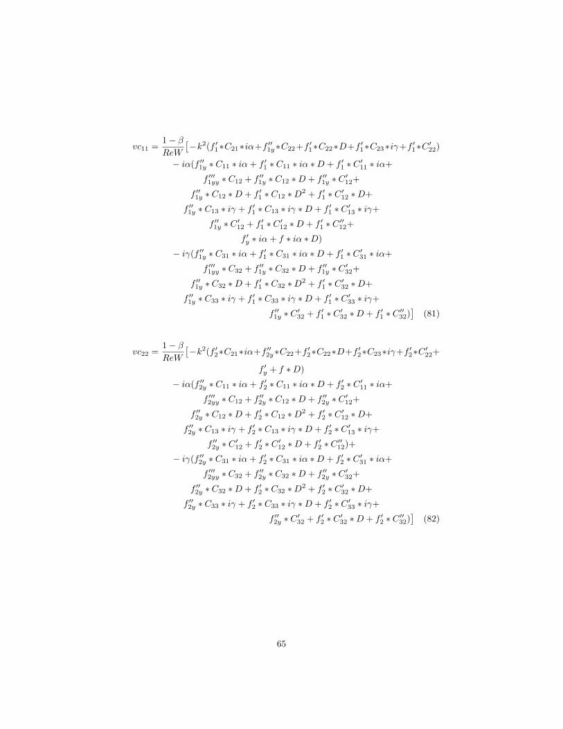
vc11 =1− βReW

[−k2(f ′1∗C21∗iα+f ′′1y ∗C22 +f ′1∗C22∗D+f ′1∗C23∗iγ+f ′1∗C ′22)

− iα(f ′′1y ∗ C11 ∗ iα+ f ′1 ∗ C11 ∗ iα ∗D + f ′1 ∗ C ′11 ∗ iα+

f ′′′1yy ∗ C12 + f ′′1y ∗ C12 ∗D + f ′′1y ∗ C ′12+

f ′′1y ∗ C12 ∗D + f ′1 ∗ C12 ∗D2 + f ′1 ∗ C ′12 ∗D+

f ′′1y ∗ C13 ∗ iγ + f ′1 ∗ C13 ∗ iγ ∗D + f ′1 ∗ C ′13 ∗ iγ+

f ′′1y ∗ C ′12 + f ′1 ∗ C ′12 ∗D + f ′1 ∗ C ′′12+

f ′y ∗ iα+ f ∗ iα ∗D)

− iγ(f ′′1y ∗ C31 ∗ iα+ f ′1 ∗ C31 ∗ iα ∗D + f ′1 ∗ C ′31 ∗ iα+

f ′′′1yy ∗ C32 + f ′′1y ∗ C32 ∗D + f ′′1y ∗ C ′32+

f ′′1y ∗ C32 ∗D + f ′1 ∗ C32 ∗D2 + f ′1 ∗ C ′32 ∗D+

f ′′1y ∗ C33 ∗ iγ + f ′1 ∗ C33 ∗ iγ ∗D + f ′1 ∗ C ′33 ∗ iγ+

f ′′1y ∗ C ′32 + f ′1 ∗ C ′32 ∗D + f ′1 ∗ C ′′32)]

(81)

vc22 =1− βReW

[−k2(f ′2∗C21∗iα+f ′′2y∗C22+f ′2∗C22∗D+f ′2∗C23∗iγ+f ′2∗C ′22+

f ′y + f ∗D)

− iα(f ′′2y ∗ C11 ∗ iα+ f ′2 ∗ C11 ∗ iα ∗D + f ′2 ∗ C ′11 ∗ iα+

f ′′′2yy ∗ C12 + f ′′2y ∗ C12 ∗D + f ′′2y ∗ C ′12+

f ′′2y ∗ C12 ∗D + f ′2 ∗ C12 ∗D2 + f ′2 ∗ C ′12 ∗D+

f ′′2y ∗ C13 ∗ iγ + f ′2 ∗ C13 ∗ iγ ∗D + f ′2 ∗ C ′13 ∗ iγ+

f ′′2y ∗ C ′12 + f ′2 ∗ C ′12 ∗D + f ′2 ∗ C ′′12)+

− iγ(f ′′2y ∗ C31 ∗ iα+ f ′2 ∗ C31 ∗ iα ∗D + f ′2 ∗ C ′31 ∗ iα+

f ′′′2yy ∗ C32 + f ′′2y ∗ C32 ∗D + f ′′2y ∗ C ′32+

f ′′2y ∗ C32 ∗D + f ′2 ∗ C32 ∗D2 + f ′2 ∗ C ′32 ∗D+

f ′′2y ∗ C33 ∗ iγ + f ′2 ∗ C33 ∗ iγ ∗D + f ′2 ∗ C ′33 ∗ iγ+

f ′′2y ∗ C ′32 + f ′2 ∗ C ′32 ∗D + f ′2 ∗ C ′′32)]

(82)

65

vc33 =1− βReW

[−k2(f ′3∗C21∗iα+f ′′3y ∗C22 +f ′3∗C22∗D+f ′3∗C23∗iγ+f ′3∗C ′22)

− iα(f ′′3y ∗ C11 ∗ iα+ f ′3 ∗ C11 ∗ iα ∗D + f ′3 ∗ C ′11 ∗ iα+

f ′′′3yy ∗ C12 + f ′′3y ∗ C12 ∗D + f ′′3y ∗ C ′12+

f ′′3y ∗ C12 ∗D + f ′3 ∗ C12 ∗D2 + f ′3 ∗ C ′12 ∗D+

f ′′3y ∗ C13 ∗ iγ + f ′3 ∗ C13 ∗ iγ ∗D + f ′3 ∗ C ′13 ∗ iγ+

f ′′3y ∗ C ′12 + f ′3 ∗ C ′12 ∗D + f ′3 ∗ C ′′12)

− iγ(f ′′3y ∗ C31 ∗ iα+ f ′3 ∗ C31 ∗ iα ∗D + f ′3 ∗ C ′31 ∗ iα+

f ′′′3yy ∗ C32 + f ′′3y ∗ C32 ∗D + f ′′3y ∗ C ′32+

f ′′3y ∗ C32 ∗D + f ′3 ∗ C32 ∗D2 + f ′3 ∗ C ′32 ∗D+

f ′′3y ∗ C33 ∗ iγ + f ′3 ∗ C33 ∗ iγ ∗D + f ′3 ∗ C ′33 ∗ iγ+

f ′′3y ∗ C ′32 + f ′3 ∗ C ′32 ∗D + f ′3 ∗ C ′′32+

f ′y ∗ iγ + f ∗ iγ ∗D)]

(83)

vc12 =1− βReW

[− k2 ∗ f ∗ iα

− iα(f ′′1y ∗ C ′11 + f ′1 ∗ C ′′11 + f ′1 ∗ C ′11 ∗D+

f ′′2y ∗ C ′22 + f ′2 ∗ C ′′22 + f ′2 ∗ C ′22 ∗D+

f ′′3y ∗ C ′33 + f ′3 ∗ C ′′33 + f ′3 ∗ C ′33 ∗D+

f ′y ∗D + f ∗D2)]

(84)

vc13 =1− βReW

[− iα(f ′y ∗ iγ + f ∗ iγ ∗ D) − iγ(f ′y ∗ iα + f ∗ iγ ∗ D)

](85)

vc23 =1− βReW

[− k2 ∗ f ∗ iγ

− iγ(f ′′1y ∗ C ′11 + f ′1 ∗ C ′′11 + f ′1 ∗ C ′11 ∗D+

f ′′2y ∗ C ′22 + f ′2 ∗ C ′′22 + f ′2 ∗ C ′22 ∗D+

f ′′3y ∗ C ′33 + f ′3 ∗ C ′′33 + f ′3 ∗ C ′33 ∗D+

f ′y ∗D + f ∗D2)]

(86)

ηc11 =1− βReW

[iγ(f ′1 ∗ C11 ∗ iα+ f ′′1y ∗ C12 + f ′1 ∗ C12 ∗D+

f ′1 ∗ C13 ∗ iγ + f ′1 ∗ C ′12 + f ∗ iα)

− iα(f ′1 ∗ C31 ∗ iα+ f ′′1y ∗ C32 + f ′1 ∗ C32 ∗D+

f ′1 ∗ C33 ∗ iγ + f ′1 ∗ C ′32)]

(87)

66

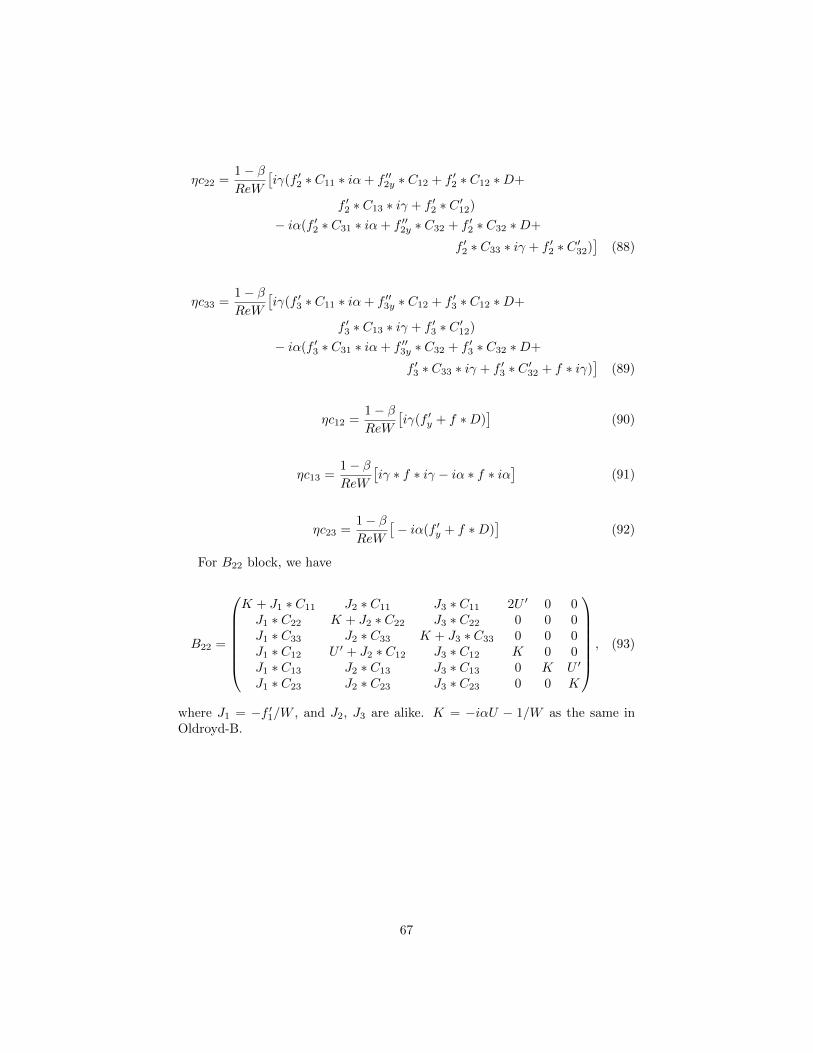
ηc22 =1− βReW

[iγ(f ′2 ∗ C11 ∗ iα+ f ′′2y ∗ C12 + f ′2 ∗ C12 ∗D+

f ′2 ∗ C13 ∗ iγ + f ′2 ∗ C ′12)

− iα(f ′2 ∗ C31 ∗ iα+ f ′′2y ∗ C32 + f ′2 ∗ C32 ∗D+

f ′2 ∗ C33 ∗ iγ + f ′2 ∗ C ′32)]

(88)

ηc33 =1− βReW

[iγ(f ′3 ∗ C11 ∗ iα+ f ′′3y ∗ C12 + f ′3 ∗ C12 ∗D+

f ′3 ∗ C13 ∗ iγ + f ′3 ∗ C ′12)

− iα(f ′3 ∗ C31 ∗ iα+ f ′′3y ∗ C32 + f ′3 ∗ C32 ∗D+

f ′3 ∗ C33 ∗ iγ + f ′3 ∗ C ′32 + f ∗ iγ)]

(89)

ηc12 =1− βReW

[iγ(f ′y + f ∗D)

](90)

ηc13 =1− βReW

[iγ ∗ f ∗ iγ − iα ∗ f ∗ iα

](91)

ηc23 =1− βReW

[− iα(f ′y + f ∗D)

](92)

For B22 block, we have

B22 =

K + J1 ∗ C11 J2 ∗ C11 J3 ∗ C11 2U ′ 0 0J1 ∗ C22 K + J2 ∗ C22 J3 ∗ C22 0 0 0J1 ∗ C33 J2 ∗ C33 K + J3 ∗ C33 0 0 0J1 ∗ C12 U ′ + J2 ∗ C12 J3 ∗ C12 K 0 0J1 ∗ C13 J2 ∗ C13 J3 ∗ C13 0 K U ′

J1 ∗ C23 J2 ∗ C23 J3 ∗ C23 0 0 K

, (93)

where J1 = −f ′1/W , and J2, J3 are alike. K = −iαU − 1/W as the same inOldroyd-B.

67

References

[1] Azaiez J., Homsy G.M., 1994 Linear stability of free shear flow of viscoelas-tic liquids. J. Fluid Mech. 268: 37-69.

[2] Azaiez J., Homsy G.M., 1994 Numerical simulation of non-Newtonian freeshear flows at high Reynolds numbers. J. Non-Newton. Fluid Mech. 52:333-374.

[3] Bistagnino A., Boffetta G., Celani A., Mazzino A., Puliafito A., VergassolaM., 2007 Nonlinear dynamics of the viscoelastic Kolmogorov flow, J. FluidMech. 590:61-80.

[4] Boffetta G., Celani A., Mazzino A., Puliafito A., Vergassola M., 2005 Theviscoelastic Kolmogorove flow: eddy viscosity and linear stability. J. FluidMech. 523:161-170.

[5] Butler K.M., Farrell B.F., 1992 Three-dimensional optimal perturbationsin viscous shear flow. Phys. Fluids 4: 1637

[6] Cadot O., Bonn D., Douady S. 1998 Turbulent drag reduction in a closedflow system: Boundary layer versus bulk effects. Phys. Fluids 10:426.

[7] Canuto C.G., Hussaini, M.Y., Quarteroni A., Zang T.A., 2007 SpectralMethods: Evolution of complex geometries and applications to fluid me-chanics.

[8] Chen J.-H., Pritchard W.G., Tavener S.J. 1995 Bifurcation for flow past acylinder between parallel planes. J. Fluid Mech. 284:23-41.

[9] Chokshi P., Kumaran V., 2009 Stability of the plane shear flow of dilutepolymeric solutions, Phys. Fluids 21: 014109.

[10] Cruz D.O.A., Pinho F.T., Oliveira P.J., 2005 Analytical solutions for fullydeveloped laminar flow of some viscoelastic liquids with a Newtonian sol-vent contribution. J. Non-Newtonian Fluid Mech. 132: 28-35.

[11] De Gennes P.G., 1990 Introduction to polymer dynamics. Cambridge uni-versity press.

[12] Dimitropoulos C.D., Dubief Y., Shaqfeh E.S.G., Moin P., Lele S.K., 2005Direct numerical simulation of polymer-induced drag reduction in turbulentboundary layer flow. Phys. Fluids 17, 011705.

[13] Dubief Y., Terrapon V.E., White C.M., Shaqfeh E.S.G., Moin P., LeleS.K., 2005 New answers on the interaction between polymers and vorticesin turbulent flows. Flow, Turbulence and Combustion 74:311-329.

[14] Dubief Y., White C.M., Terrapon V.E., Shaqfeh E.S.G., Moin P., Lele S.K.,2004 On the coherent drag-reducing and turbulence-enhancing behaviourof polymers in wall flows. J. Fluid Mech. 514:271-280.

68

[15] Farrell B.F., 1988 Optimal excitation of perturbations in viscous shear flow,Phys. Fluids 31: 2093-2102.

[16] Farrell B.F., Ioannou P.J., Optimal excitation of three-dimensional pertur-bations in viscous constant shear flow. Phys. Fluids 5: 1390.

[17] Govindarajan R., 2004 Effect of miscibility on the linear instability of two-fluid channel flow. Int. J. Multiphase Flow 30: 1177-1192.

[18] Groisman A., Steinberg V. 2000 Elastic turbulence in a polymer solutionflow. Nature 405: 53-55.

[19] Hamilton J.M., Kim J., Waleffe F., 1995 Regeneration mechanisms of near-wall turbulence structures. J. Fluid Mech. 287:317-348.

[20] Hinch E.J., 1977 Mechanical models of dilute polymer solutions in strongflows. Phys. Fluids 20:s22-s33.

[21] Hoda N., Jovanovic M.R., Kumar S. 2008 Energy amplification in channelflows of viscoelastic fluids. J. Fluid Mech. 601: 407-424.

[22] James D. 2009 Boger fluids. Annu. Rev. Fluid Mech. 41:129-42.

[23] Jimenez J., Moin P. 1991 The minimal flow unit in near wall turbulence.J. Fluid Mech. 225: 221-240

[24] Jimenez J., Pinelli A., 1999 The autonomous cycle of near-wall turbulence.J. Fluid Mech. 389:335-359.

[25] Klinkenberg J., de Lange H.C., Brandt L., 2011 Modal and non-modalstability of particle-laden channel flow. Phys. Fluids 23:064110.

[26] Jovanovic M.R., Kumar S., 2010 Transient growth without inertia. Phys.Fluids 22:023101.

[27] Jovanovic M.R., Kumar S., 2011 Nonmodal amplification of stochastic dis-turbances in strongly elastic channel flows. J. Non-Newtonian Fluid Mech.166:755:778.

[28] Larson R.G. 1992 Instabilities in viscoelastic flows. Rheol. Acta 31:213-63.

[29] Larson R.G., Shaqfeh E.S.G., Muller S.J. 1990 A purely elastic instabilityin Taylor-Couette flow. J. Fluid Mech. 218:573-600.

[30] Lumley J.L., 1969 Drag reduction by additives. Annu. Rev. Fluid Mech.1:367-384.

[31] Lumley J.L., 1973 Drag reduction in turbulent flow by polymer additives.J. Polymer Sci. Macromol. Rev. 7:263-290.

[32] Min T., Yoo J.Y., Choi H., Joseph D.D., 2003 Drag reduction by polymeradditives in a turbulent channel flow. J. Fluid Mech. 486:213-238.

69

[33] Nouar C., Bottaro A., Brancher J.P., 2007 Delaying transition to turbulencein channel flow: revisiting the stability of shear-thinning fluids. J. FluidMech. 592:177-194.

[34] Petrie C.J.S., Denn M.M., 1976 Instabilities in polymer processing. AIChEJ. 22:209-36.

[35] Phan-Thien N. 1983 Coaxial-disk flow of an Oldroyd-B fluid: exact solutionand stability. J. Non-Newton. Fluid Mech. 13:325-40

[36] Porteous K.C., Denn M.M., 1972 Linear stability of plane Poiseuille flowof viscoelastic liquids Trans. Soc. Rheol. 16:295-308.

[37] Rallison J.M., Hinch E.J., 1995 Instability of a high-speed submerged elas-tic jet. J. Fluid Mech. 288 :311-324.

[38] Reddy S.C., Schmid P.J., Henningson, D.S., Pseudospectra of the Orr-Sommerfeld operator. SIAM J. Appl. Math. 53: 15-47.

[39] Rees S.J., Juniper M.P., The effect of confinement on the stability of viscousplanar jets and wakes. J. Fluid Mech. 656 :309-336.

[40] Sadanandan B., Sureshkumar R., 2002 Viscoelastic effects on the stabilityof wall-bounded shear flows. Phys. Fluids 14:41-48. dfweefw

[41] Schmid P. J., Henningson D.S., Stability and transition in shear flows.Springer 2001.

[42] Shaqfeh E.S.G., Purely elastic instabilities in viscometric flows. Annu. Rev.Fluid Mech. 28: 129-185.

[43] Sureshkumar R., Beris A.N. 1995 Linear stability analysis of viscoelasticPoiseuille flow using an Arnoldi-based orthogonalization algorithm. J. Non-Newtonian Fluid Mech. 56: 151-182. svfwrfw

[44] Trefethen L.N., Spectral methods in MATLAB, SIAM, Philadelphia, 2000.

[45] Warholic M.D., Massah H., Hanratty T.J., 1999 Influence of drag-reducingpolymers on turbulence: effects of Reynolds number, concentration andmixing. Experiments in Fluids 27:461-472.

[46] Weideman J.A., Reddy S.C., 2000 A MATLAB differentiation matrix suite.ACM TOMS 26: 465-519.

70