SW Ch 4 1/42

Linear Regression with One Regressor

(Stock/Watson Chapter 4)

Outline

1. The population linear regression model

2. The ordinary least squares (OLS) estimator and the

sample regression line

3. Measures of fit of the sample regression

4. The least squares assumptions

5. The sampling distribution of the OLS estimator

SW Ch 4 2/42

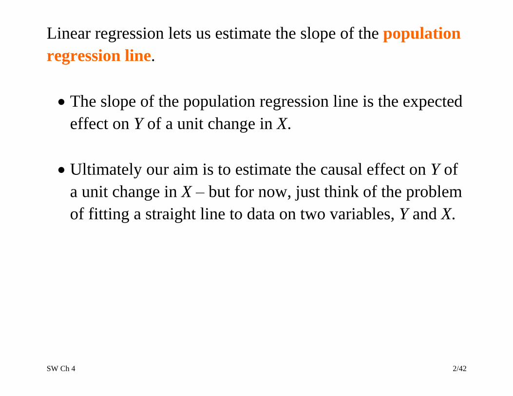
Linear regression lets us estimate the slope of the population

regression line.

• The slope of the population regression line is the expected

effect on Y of a unit change in X.

• Ultimately our aim is to estimate the causal effect on Y of

a unit change in X – but for now, just think of the problem

of fitting a straight line to data on two variables, Y and X.

SW Ch 4 3/42

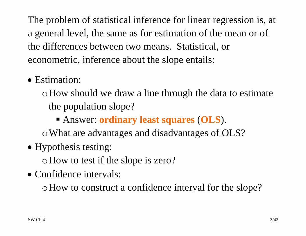
The problem of statistical inference for linear regression is, at

a general level, the same as for estimation of the mean or of

the differences between two means. Statistical, or

econometric, inference about the slope entails:

• Estimation:

o How should we draw a line through the data to estimate

the population slope?

▪ Answer: ordinary least squares (OLS).

o What are advantages and disadvantages of OLS?

• Hypothesis testing:

o How to test if the slope is zero?

• Confidence intervals:

o How to construct a confidence interval for the slope?

SW Ch 4 4/42

The Linear Regression Model

(SW Section 4.1)

The population regression line:

Test Score = 0 + 1STR

1 = slope of population regression line

= Test score

STR

= change in test score for a unit change in STR

• Why are 0 and 1 “population” parameters?

• We would like to know the population value of 1.

• We don’t know 1, so must estimate it using data.

SW Ch 4 5/42

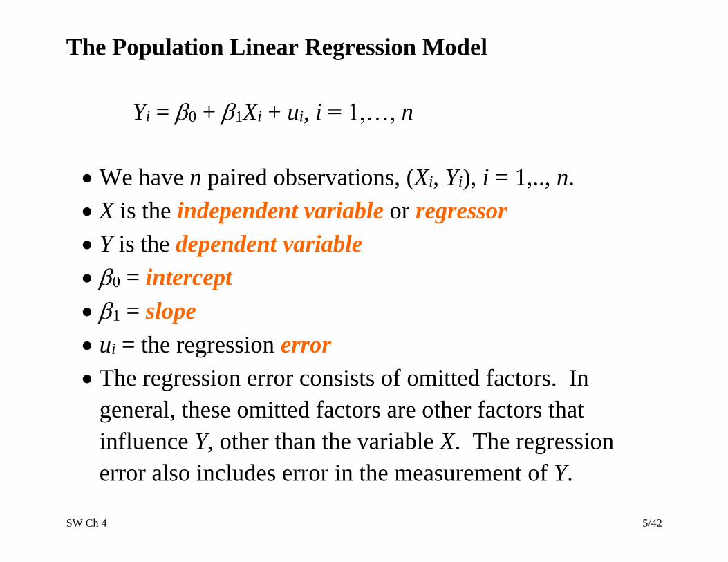
The Population Linear Regression Model

Yi = 0 + 1Xi + ui, i = 1,…, n

• We have n paired observations, (Xi, Yi), i = 1,.., n.

• X is the independent variable or regressor

• Y is the dependent variable

• 0 = intercept

• 1 = slope

• ui = the regression error

• The regression error consists of omitted factors. In

general, these omitted factors are other factors that

influence Y, other than the variable X. The regression

error also includes error in the measurement of Y.

SW Ch 4 6/42

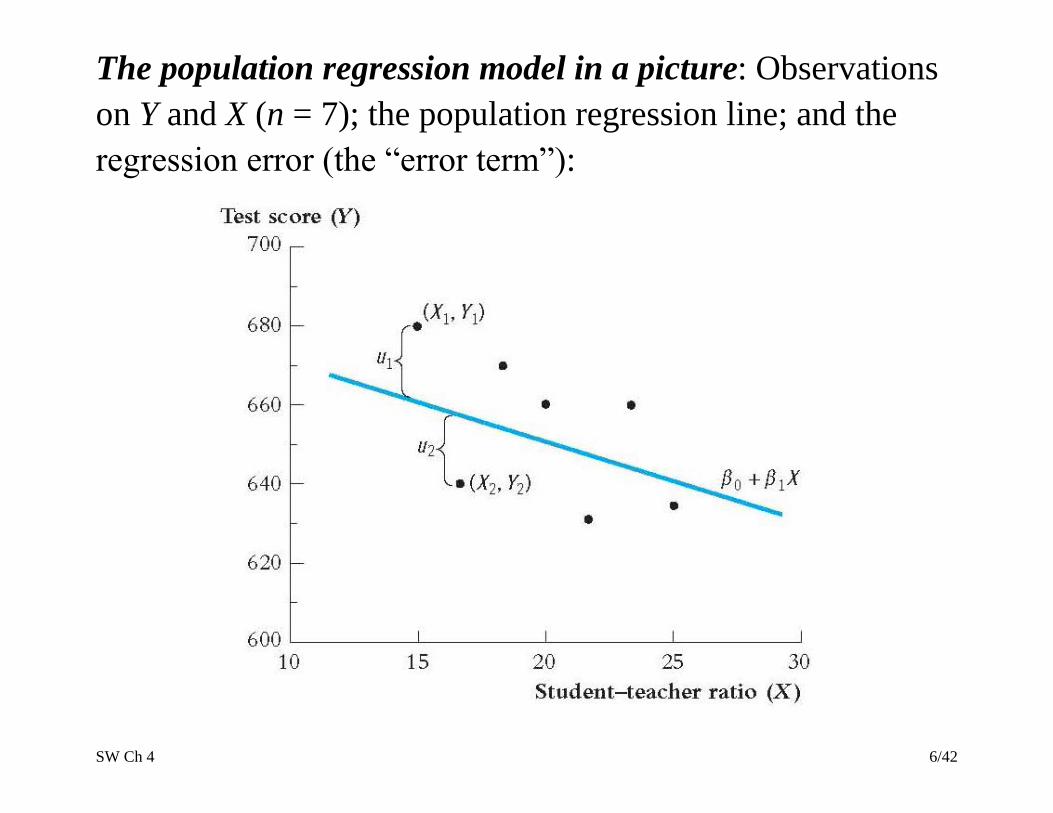
The population regression model in a picture: Observations

on Y and X (n = 7); the population regression line; and the

regression error (the “error term”):

SW Ch 4 7/42

The Ordinary Least Squares Estimator

(SW Section 4.2)

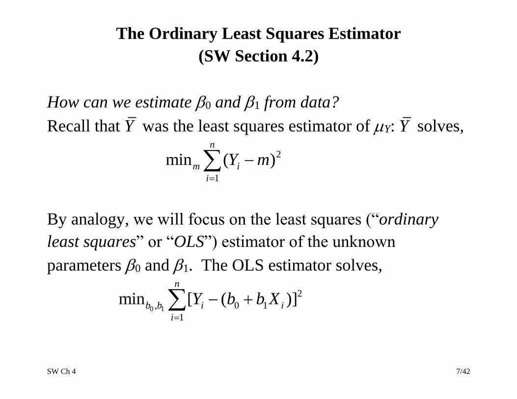
How can we estimate 0 and 1 from data?

Recall that Y was the least squares estimator of Y: Y solves,

2

1

min ( )n

m i

i

Y m

By analogy, we will focus on the least squares (“ordinary

least squares” or “OLS”) estimator of the unknown

parameters 0 and 1. The OLS estimator solves,

0 1

2

, 0 1

1

min [ ( )]n

b b i i

i

Y b b X

SW Ch 4 8/42

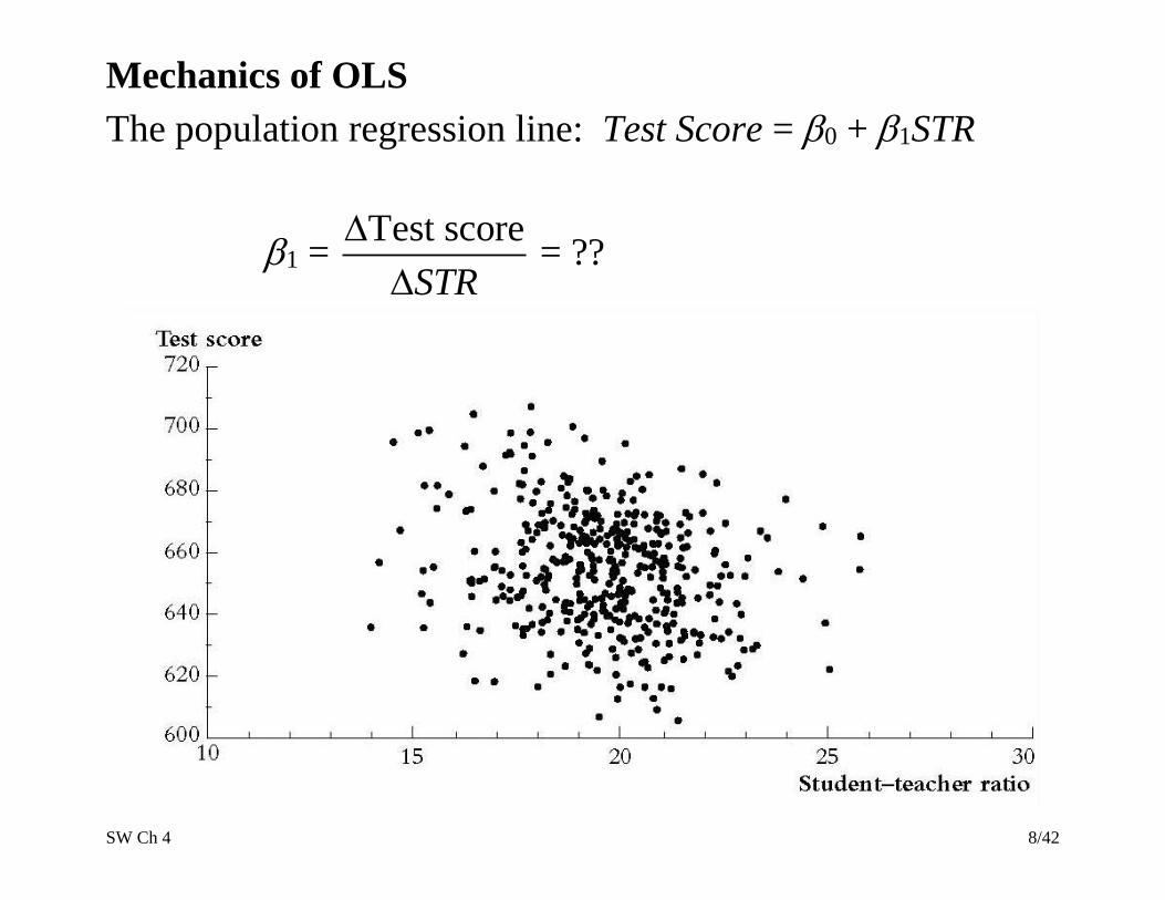
Mechanics of OLS

The population regression line: Test Score = 0 + 1STR

1 = Test score

STR

= ??

SW Ch 4 9/42

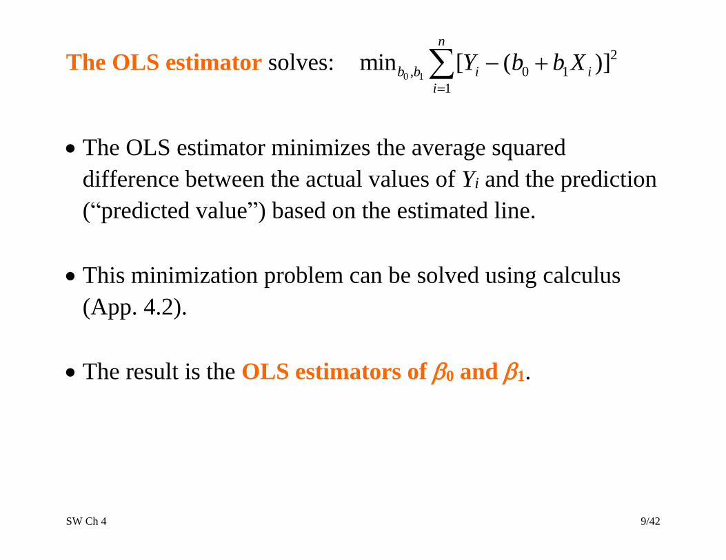
The OLS estimator solves: 0 1

2

, 0 1

1

min [ ( )]n

b b i i

i

Y b b X

• The OLS estimator minimizes the average squared

difference between the actual values of Yi and the prediction

(“predicted value”) based on the estimated line.

• This minimization problem can be solved using calculus

(App. 4.2).

• The result is the OLS estimators of 0 and 1.

SW Ch 4 10/42

SW Ch 4 11/42

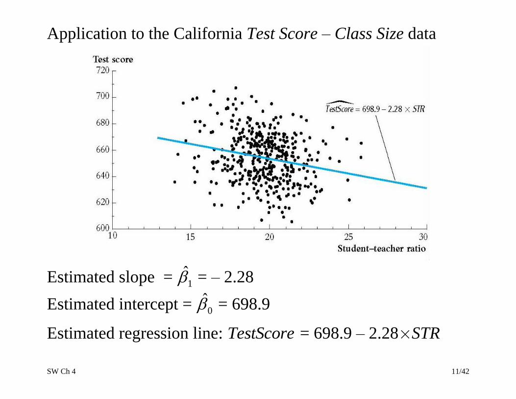
Application to the California Test Score – Class Size data

Estimated slope = 1 = – 2.28

Estimated intercept = 0 = 698.9

Estimated regression line: TestScore = 698.9 – 2.28STR

SW Ch 4 12/42

Interpretation of the estimated slope and intercept

TestScore = 698.9 – 2.28STR

• Districts with one more student per teacher on average

have test scores that are 2.28 points lower.

• That is, Test score

STR

= –2.28

• The intercept (taken literally) means that, according to this

estimated line, districts with zero students per teacher

would have a (predicted) test score of 698.9. But this

interpretation of the intercept makes no sense – it

extrapolates the line outside the range of the data – here,

the intercept is not economically meaningful.

SW Ch 4 13/42

Predicted values & residuals:

One of the districts in the data set is Antelope, CA, for which

STR = 19.33 and Test Score = 657.8

predicted value: ˆAntelopeY = 698.9 – 2.2819.33 = 654.8

residual: ˆAntelopeu = 657.8 – 654.8 = 3.0

SW Ch 4 14/42

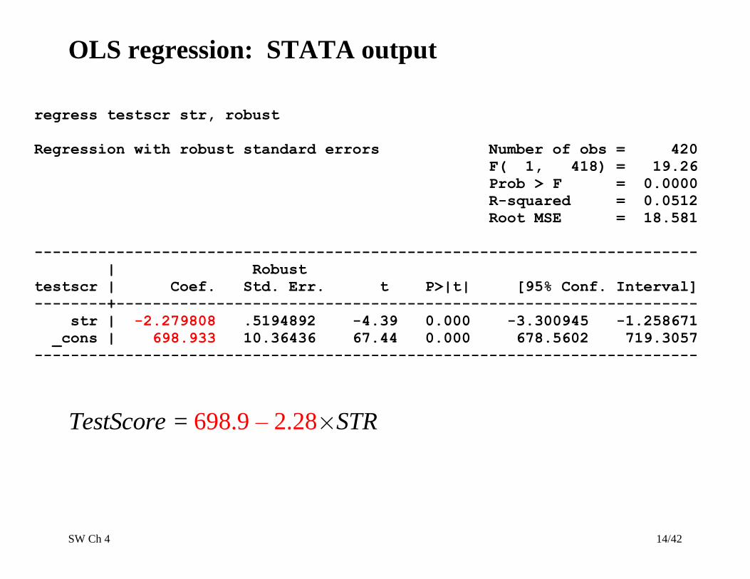
OLS regression: STATA output

regress testscr str, robust

Regression with robust standard errors Number of obs = 420

F( 1, 418) = 19.26

Prob > F = 0.0000

R-squared = 0.0512

Root MSE = 18.581

-------------------------------------------------------------------------

| Robust

testscr | Coef. Std. Err. t P>|t| [95% Conf. Interval]

--------+----------------------------------------------------------------

str | -2.279808 .5194892 -4.39 0.000 -3.300945 -1.258671

_cons | 698.933 10.36436 67.44 0.000 678.5602 719.3057

-------------------------------------------------------------------------

TestScore = 698.9 – 2.28STR

SW Ch 4 15/42

Measures of Fit

(Section 4.3)

Two regression statistics provide complementary measures of

how well the regression line “fits” or explains the data:

• The regression R2 measures the fraction of the variance of

Y that is explained by X; it is unitless and ranges between

zero (no fit) and one (perfect fit)

• The standard error of the regression (SER) measures the

magnitude of a typical regression residual in the units of

Y.

SW Ch 4 16/42

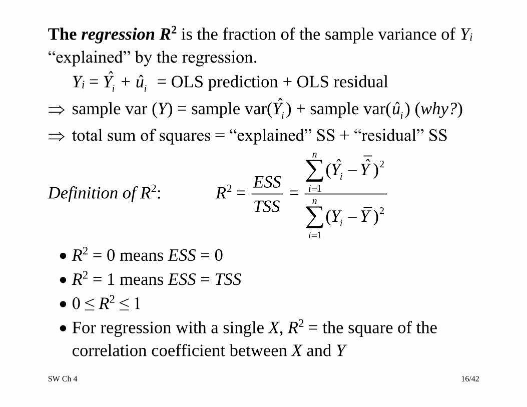
The regression R2 is the fraction of the sample variance of Yi

“explained” by the regression.

Yi = ˆiY + ˆ

iu = OLS prediction + OLS residual

sample var (Y) = sample var( ˆiY ) + sample var( ˆ

iu ) (why?)

total sum of squares = “explained” SS + “residual” SS

Definition of R2: R2 = ESS

TSS =

2

1

2

1

ˆ ˆ( )

( )

n

i

i

n

i

i

Y Y

Y Y

• R2 = 0 means ESS = 0

• R2 = 1 means ESS = TSS

• 0 ≤ R2 ≤ 1

• For regression with a single X, R2 = the square of the

correlation coefficient between X and Y

SW Ch 4 17/42

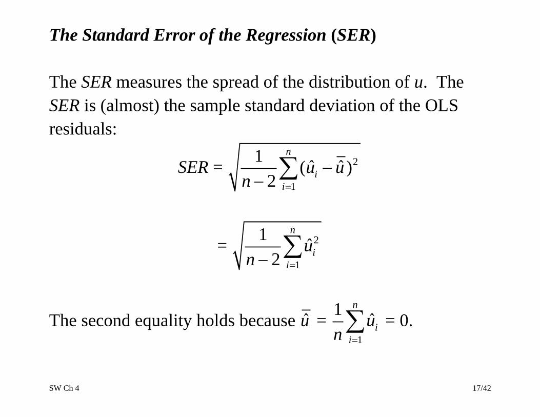
The Standard Error of the Regression (SER)

The SER measures the spread of the distribution of u. The

SER is (almost) the sample standard deviation of the OLS

residuals:

SER = 2

1

1ˆ ˆ( )

2

n

i

i

u un

= 2

1

1ˆ

2

n

i

i

un

The second equality holds because u = 1

1ˆ

n

i

i

un

= 0.

SW Ch 4 18/42

SER = 2

1

1ˆ

2

n

i

i

un

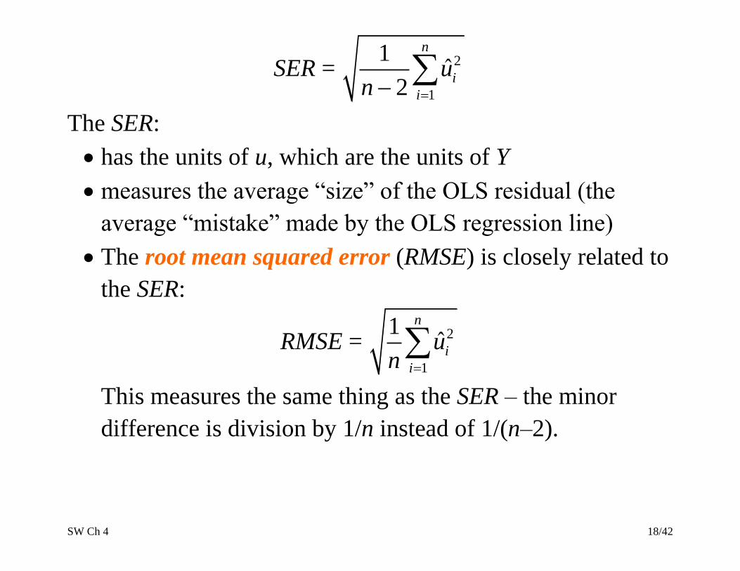
The SER:

• has the units of u, which are the units of Y

• measures the average “size” of the OLS residual (the

average “mistake” made by the OLS regression line)

• The root mean squared error (RMSE) is closely related to

the SER:

RMSE = 2

1

1ˆ

n

i

i

un

This measures the same thing as the SER – the minor

difference is division by 1/n instead of 1/(n–2).

SW Ch 4 19/42

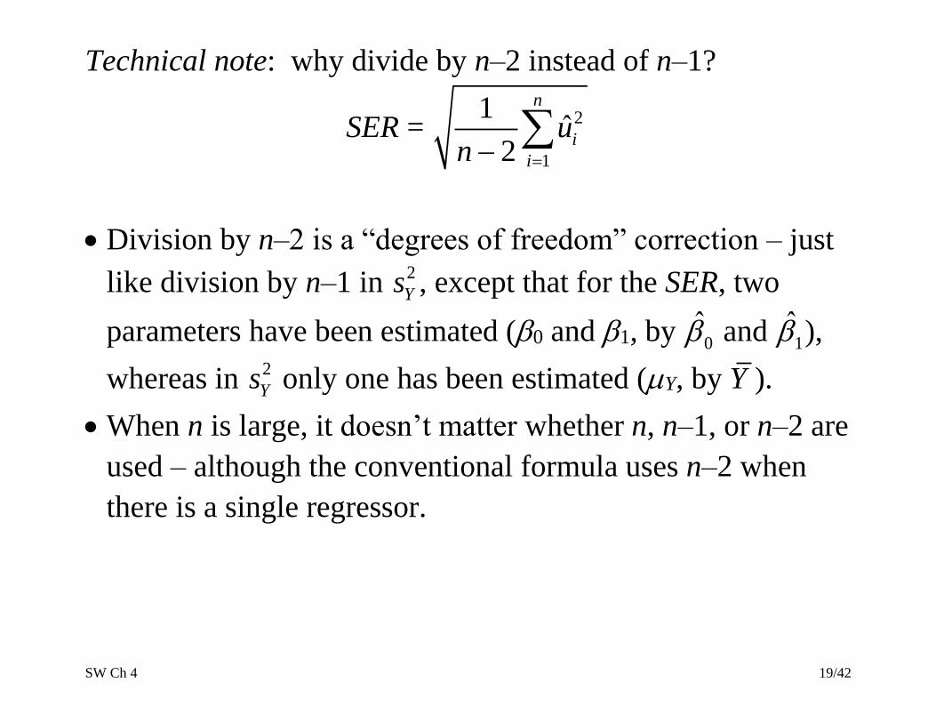
Technical note: why divide by n–2 instead of n–1?

SER = 2

1

1ˆ

2

n

i

i

un

• Division by n–2 is a “degrees of freedom” correction – just

like division by n–1 in 2

Ys , except that for the SER, two

parameters have been estimated (0 and 1, by 0 and 1 ),

whereas in 2

Ys only one has been estimated (Y, by Y ).

• When n is large, it doesn’t matter whether n, n–1, or n–2 are

used – although the conventional formula uses n–2 when

there is a single regressor.

SW Ch 4 20/42

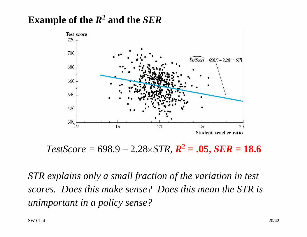
Example of the R2 and the SER

TestScore = 698.9 – 2.28STR, R2 = .05, SER = 18.6

STR explains only a small fraction of the variation in test

scores. Does this make sense? Does this mean the STR is

unimportant in a policy sense?

SW Ch 4 21/42

The Least Squares Assumptions

(SW Section 4.4)

What, in a precise sense, are the properties of the

sampling distribution of the OLS estimator? When will 1 be

unbiased? What is its variance?

To answer these questions, we need to make some

assumptions about how Y and X are related to each other, and

about how they are collected (the sampling scheme)

These assumptions – there are three – are known as the

Least Squares Assumptions.

SW Ch 4 22/42

The Least Squares Assumptions

Yi = 0 + 1Xi + ui, i = 1,…, n

1. The conditional distribution of u given X has mean zero,

that is, E(u|X = x) = 0.

• This implies that 1 is unbiased

2. (Xi,Yi), i =1,…,n, are i.i.d.

• This is true if (X, Y) are collected by simple random

sampling

• This delivers the sampling distribution of 0 and 1

3. Large outliers in X and/or Y are rare.

• Technically, X and Y have finite fourth moments

• Outliers can result in meaningless values of 1

SW Ch 4 23/42

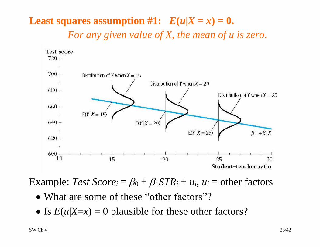
Least squares assumption #1: E(u|X = x) = 0.

For any given value of X, the mean of u is zero.

Example: Test Scorei = 0 + 1STRi + ui, ui = other factors

• What are some of these “other factors”?

• Is E(u|X=x) = 0 plausible for these other factors?

SW Ch 4 24/42

Least squares assumption #1, ctd.

A benchmark for thinking about this assumption is to

consider an ideal randomized controlled experiment:

• X is randomly assigned to people (students randomly

assigned to different size classes; patients randomly

assigned to medical treatments). Randomization is done

by computer – using no information about the individual.

• Because X is assigned randomly, all other individual

characteristics – the things that make up u – are

distributed independently of X, so u and X are independent

• Thus, in an ideal randomized controlled experiment,

E(u|X = x) = 0 (that is, LSA #1 holds)

• In actual experiments, or with observational data, we will

need to think hard about whether E(u|X = x) = 0 holds.

SW Ch 4 25/42

Least squares assumption #2: (Xi, Yi), i = 1,…,n are i.i.d.

This arises automatically if the entity (individual, district)

is sampled by simple random sampling:

• The entities are selected from the same population, so

(Xi, Yi) are identically distributed for all i = 1,…, n.

• The entities are selected at random, so the values of (X,

Y) for different entities are independently distributed.

The main place we will encounter non-i.i.d. sampling is

when data are recorded over time for the same entity (panel

data and time series data) – we will deal with that

complication when we cover panel data.

SW Ch 4 26/42

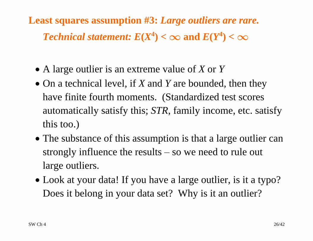
Least squares assumption #3: Large outliers are rare.

Technical statement: E(X4) < and E(Y4) <

• A large outlier is an extreme value of X or Y

• On a technical level, if X and Y are bounded, then they

have finite fourth moments. (Standardized test scores

automatically satisfy this; STR, family income, etc. satisfy

this too.)

• The substance of this assumption is that a large outlier can

strongly influence the results – so we need to rule out

large outliers.

• Look at your data! If you have a large outlier, is it a typo?

Does it belong in your data set? Why is it an outlier?

SW Ch 4 27/42

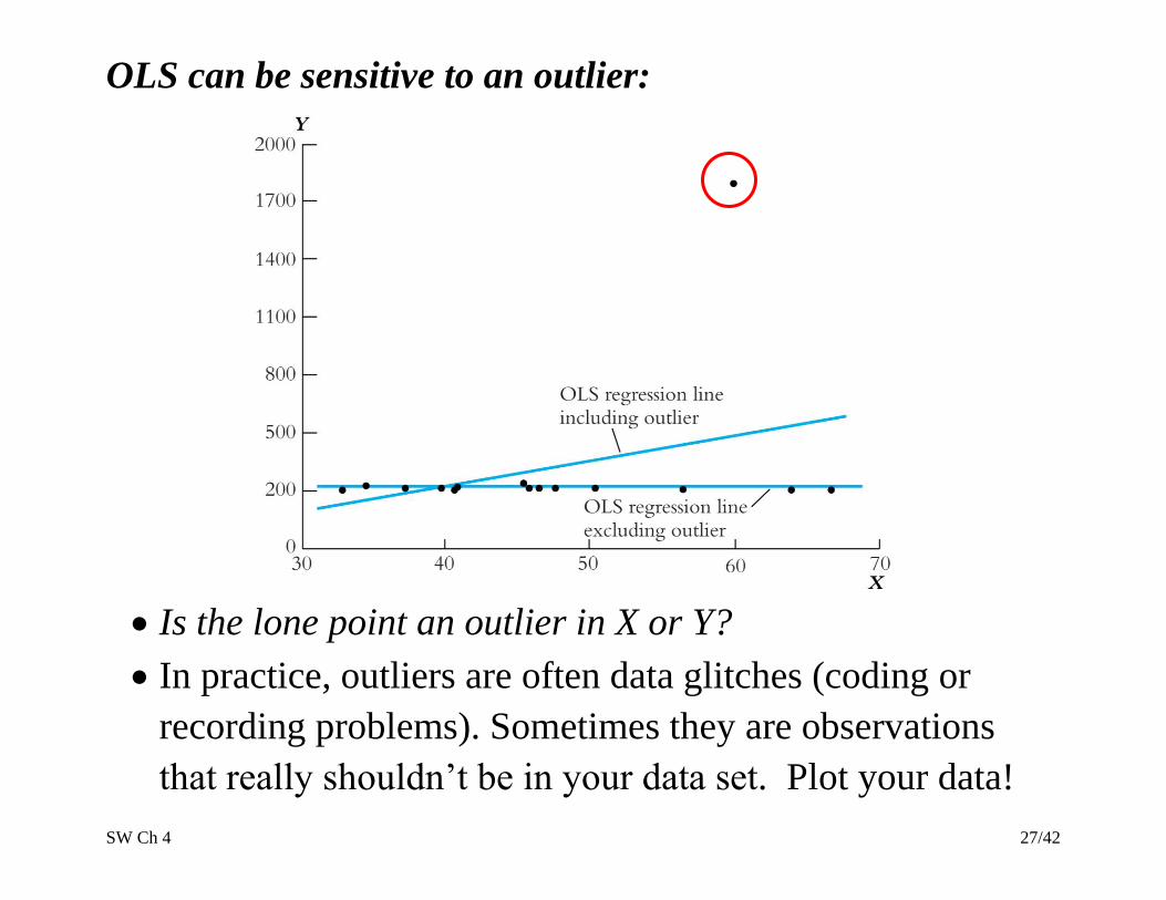
OLS can be sensitive to an outlier:

• Is the lone point an outlier in X or Y?

• In practice, outliers are often data glitches (coding or

recording problems). Sometimes they are observations

that really shouldn’t be in your data set. Plot your data!

SW Ch 4 28/42

The Sampling Distribution of the OLS Estimator

(SW Section 4.5)

The OLS estimator is computed from a sample of data. A

different sample yields a different value of 1 . This is the

source of the “sampling uncertainty” of 1 . We want to:

• quantify the sampling uncertainty associated with 1

• use 1 to test hypotheses such as 1 = 0

• construct a confidence interval for 1

• All these require figuring out the sampling distribution of

the OLS estimator. Two steps to get there…

o Probability framework for linear regression

o Distribution of the OLS estimator

SW Ch 4 29/42

Probability Framework for Linear Regression

The probability framework for linear regression is

summarized by the three least squares assumptions.

Population

• The group of interest (ex: all possible school districts)

Random variables: Y, X

• Ex: (Test Score, STR)

Joint distribution of (Y, X). We assume:

• The population regression function is linear

• E(u|X) = 0 (1st Least Squares Assumption)

• X, Y have nonzero finite fourth moments (3rd L.S.A.)

Data Collection by simple random sampling implies

• {(Xi, Yi)}, i = 1,…, n, are i.i.d. (2nd L.S.A.)

SW Ch 4 30/42

The Sampling Distribution of 1

Like Y , 1 has a sampling distribution.

• What is E( 1 )?

o If E( 1 ) = 1, then OLS is unbiased – a good thing!

• What is var( 1 )? (measure of sampling uncertainty)

o We need to derive a formula so we can compute the

standard error of 1 .

• What is the distribution of 1 in small samples?

o It is very complicated in general

• What is the distribution of 1 in large samples?

o In large samples, 1 is normally distributed.

SW Ch 4 31/42

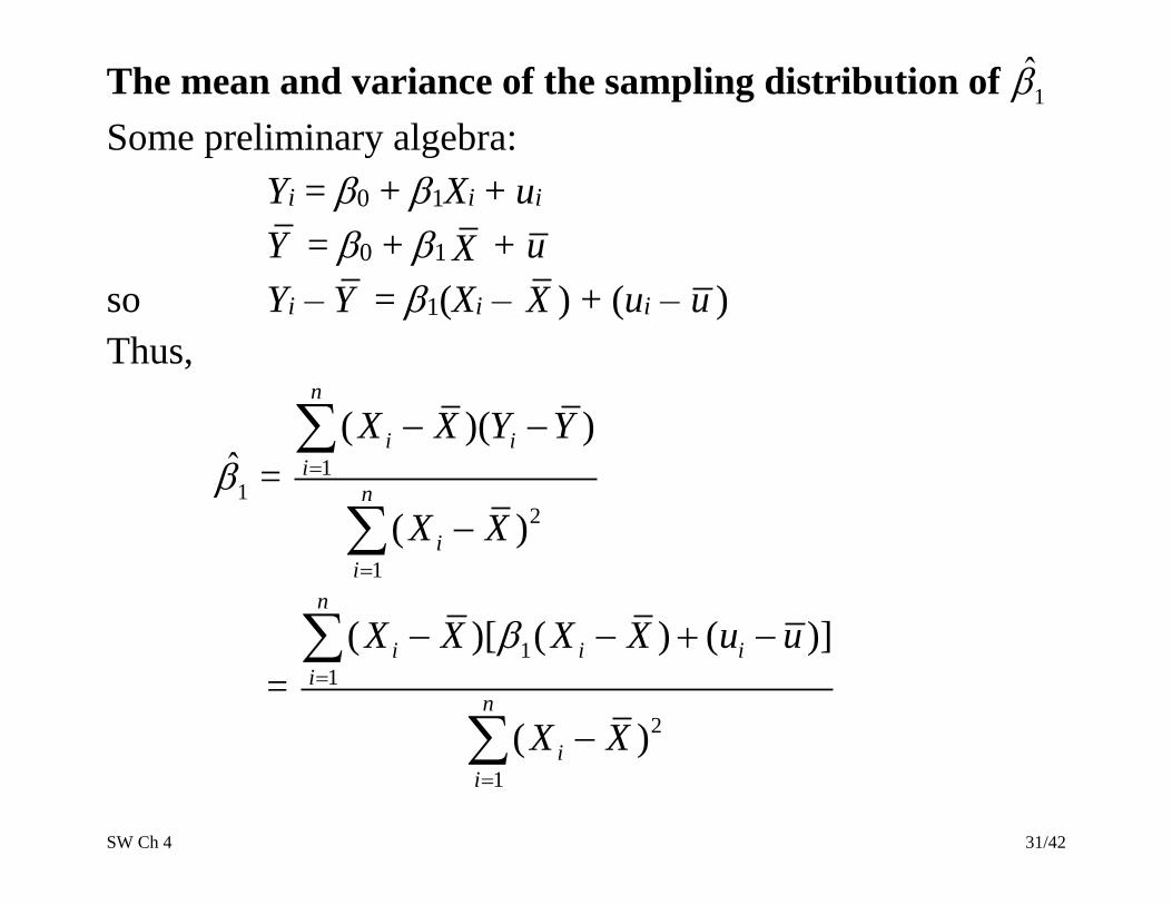
The mean and variance of the sampling distribution of 1

Some preliminary algebra:

Yi = 0 + 1Xi + ui

Y = 0 + 1 X + u

so Yi – Y = 1(Xi – X ) + (ui – u )

Thus,

1 = 1

2

1

( )( )

( )

n

i i

i

n

i

i

X X Y Y

X X

= 1

1

2

1

( )[ ( ) ( )]

( )

n

i i i

i

n

i

i

X X X X u u

X X

SW Ch 4 32/42

1 = 1 11

2 2

1 1

( )( ) ( )( )

( ) ( )

n n

i i i i

i i

n n

i i

i i

X X X X X X u u

X X X X

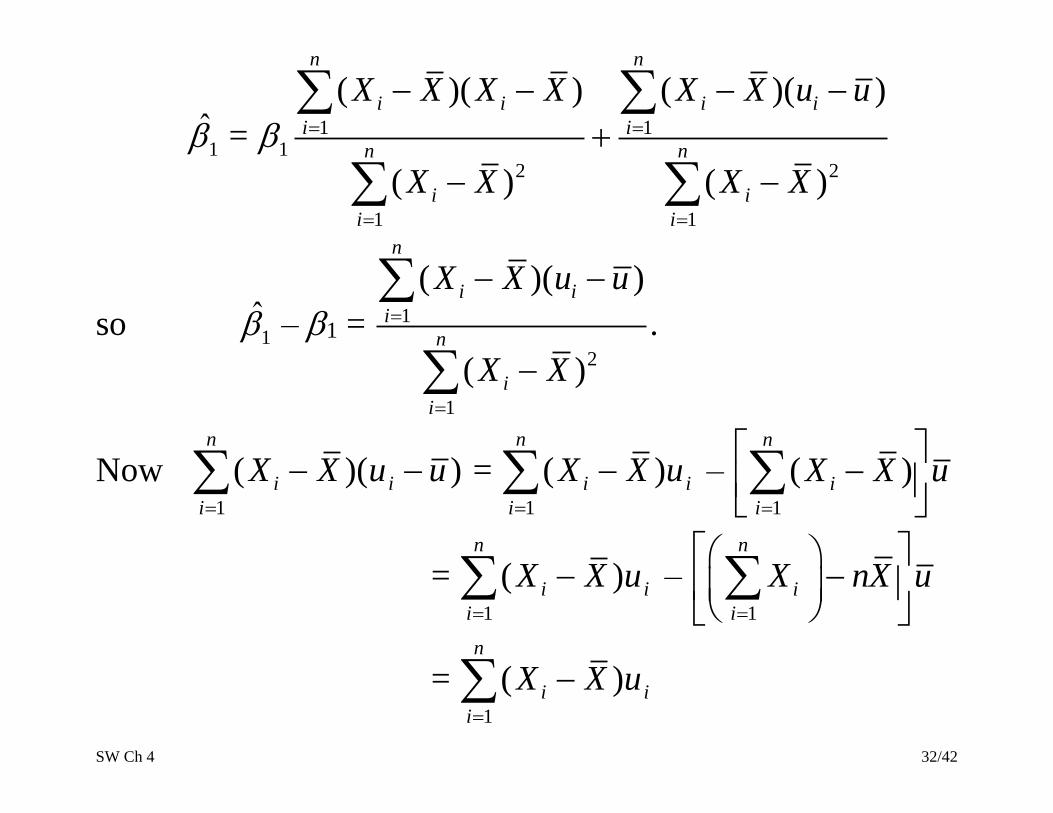
so 1 – 1 = 1

2

1

( )( )

( )

n

i i

i

n

i

i

X X u u

X X

.

Now 1

( )( )n

i i

i

X X u u

= 1

( )n

i i

i

X X u

– 1

( )n

i

i

X X u

= 1

( )n

i i

i

X X u

– 1

n

i

i

X nX u

= 1

( )n

i i

i

X X u

SW Ch 4 33/42

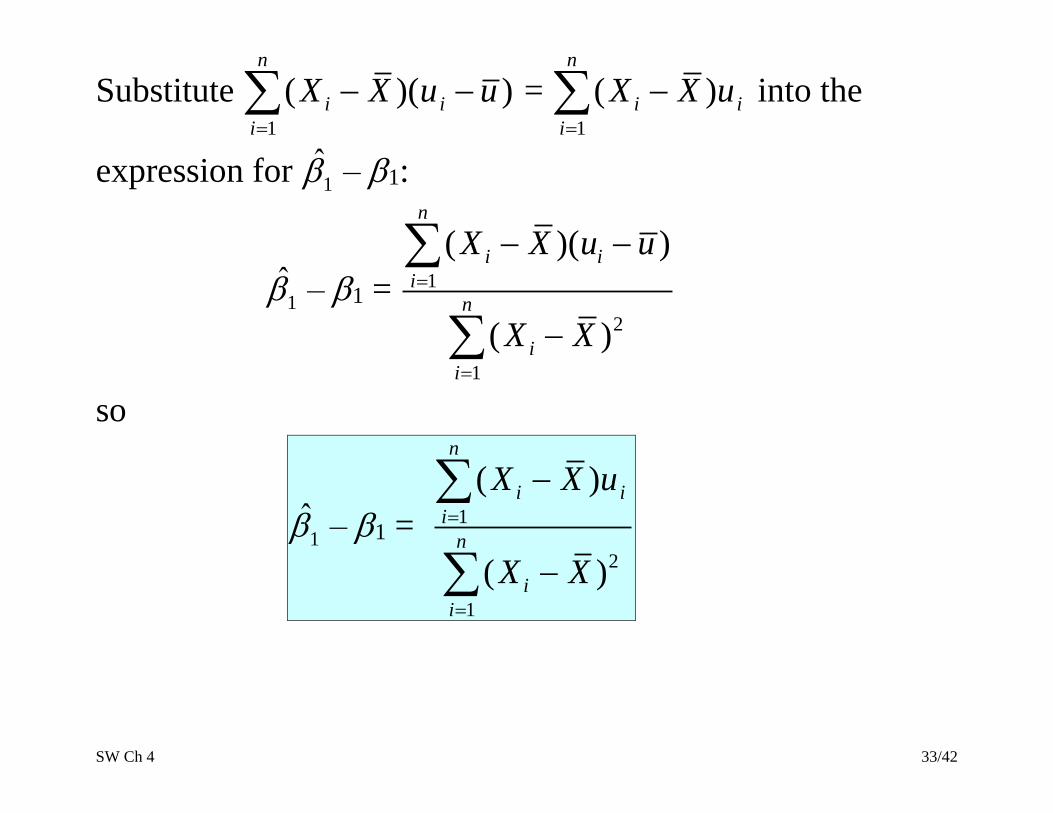
Substitute 1

( )( )n

i i

i

X X u u

= 1

( )n

i i

i

X X u

into the

expression for 1 – 1:

1 – 1 = 1

2

1

( )( )

( )

n

i i

i

n

i

i

X X u u

X X

so

1 – 1 = 1

2

1

( )

( )

n

i i

i

n

i

i

X X u

X X

SW Ch 4 34/42

Now we can calculate E( 1 ) and var( 1 ):

E( 1 ) – 1 = 1

2

1

( )

( )

n

i i

i

n

i

i

X X u

E

X X

= 11

2

1

( )

,...,

( )

n

i i

inn

i

i

X X u

E E X X

X X

= 0 because E(ui|Xi=x) = 0 by LSA #1

• Thus LSA #1 implies that E( 1 ) = 1

• That is, 1 is an unbiased estimator of 1.

SW Ch 4 35/42

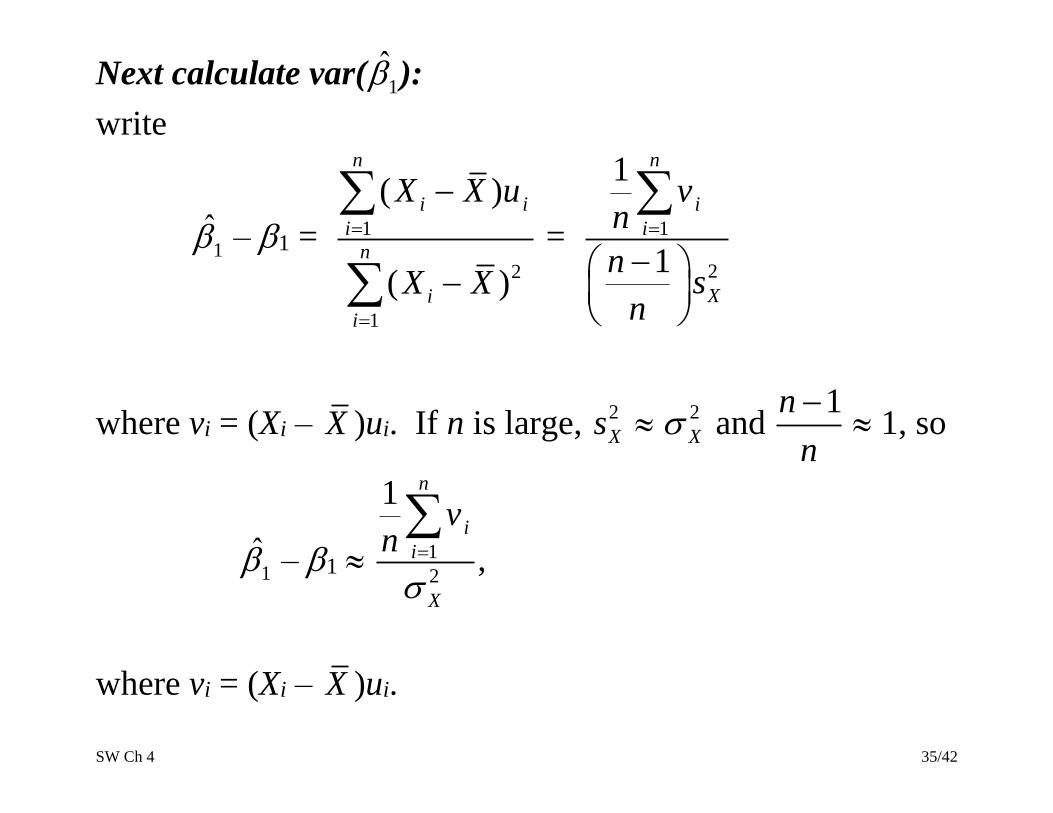
Next calculate var( 1 ):

write

1 – 1 = 1

2

1

( )

( )

n

i i

i

n

i

i

X X u

X X

= 1

2

1

1

n

i

i

X

vn

ns

n

where vi = (Xi – X )ui. If n is large, 2

Xs 2

X and 1n

n

1, so

1 – 1 1

2

1 n

i

i

X

vn

,

where vi = (Xi – X )ui.

SW Ch 4 36/42

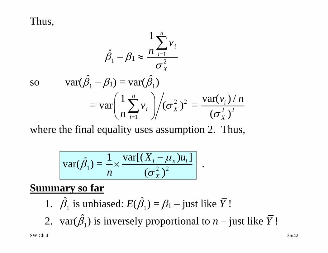
Thus,

1 – 1 1

2

1 n

i

i

X

vn

so var( 1 – 1) = var( 1 )

= 2 2

1

1var ( )

n

i X

i

vn

=

2 2

var( ) /

( )

i

X

v n

where the final equality uses assumption 2. Thus,

var( 1 ) = 2 2

var[( ) ]1

( )

i x i

X

X u

n

.

Summary so far

1. 1 is unbiased: E( 1 ) = 1 – just like Y !

2. var( 1 ) is inversely proportional to n – just like Y !

SW Ch 4 37/42

What is the sampling distribution of 1 ?

The exact sampling distribution is complicated – it

depends on the population distribution of (Y, X) – but when n

is large we get some simple (and good) approximations:

(1) Because var( 1 ) 1/n and E( 1 ) = 1, 1 p

1

(2) When n is large, the sampling distribution of 1 is

well approximated by a normal distribution (CLT)

Recall the CLT: suppose {vi}, i = 1,…, n is i.i.d. with E(v) =

0 and var(v) = 2. Then, when n is large, 1

1 n

i

i

vn

is

approximately distributed N(0, 2 /v n ).

SW Ch 4 38/42

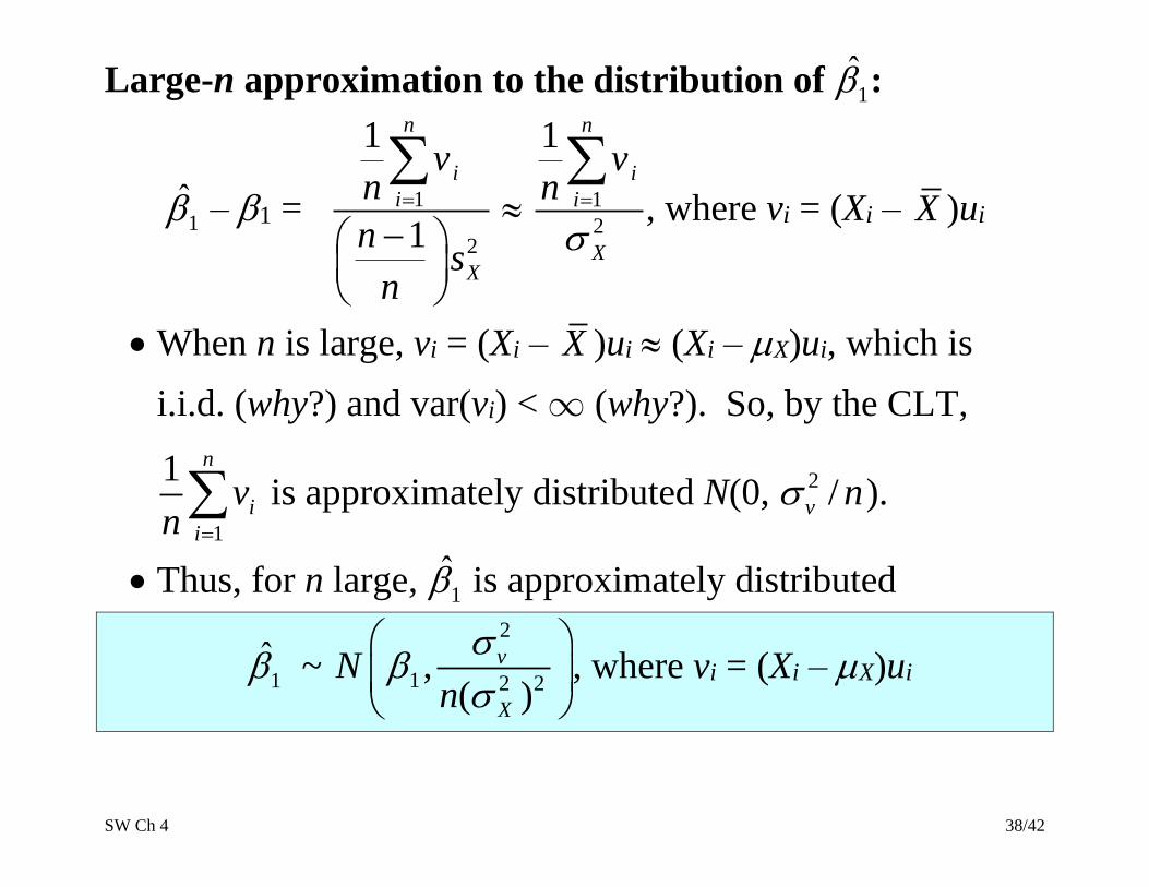
Large-n approximation to the distribution of 1 :

1 – 1 = 1

2

1

1

n

i

i

X

vn

ns

n

1

2

1 n

i

i

X

vn

, where vi = (Xi – X )ui

• When n is large, vi = (Xi – X )ui (Xi – X)ui, which is

i.i.d. (why?) and var(vi) < (why?). So, by the CLT,

1

1 n

i

i

vn

is approximately distributed N(0, 2 /v n ).

• Thus, for n large, 1 is approximately distributed

1 ~ 2

1 2 2,

( )

v

X

Nn

, where vi = (Xi – X)ui

SW Ch 4 39/42

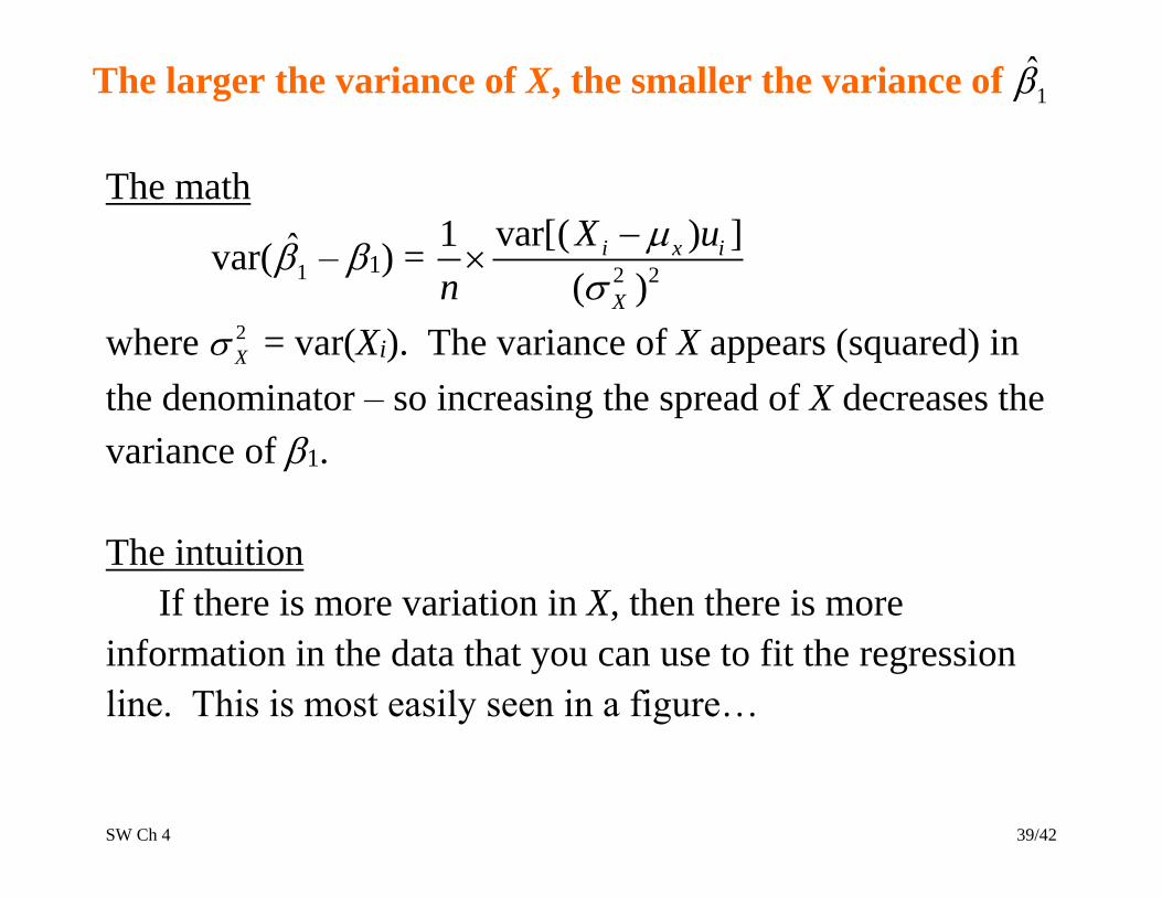
The larger the variance of X, the smaller the variance of 1

The math

var( 1 – 1) = 2 2

var[( ) ]1

( )

i x i

X

X u

n

where 2

X = var(Xi). The variance of X appears (squared) in

the denominator – so increasing the spread of X decreases the

variance of 1.

The intuition

If there is more variation in X, then there is more

information in the data that you can use to fit the regression

line. This is most easily seen in a figure…

SW Ch 4 40/42

The larger the variance of X, the smaller the variance of 1

The number of black and blue dots is the same. Using which

would you get a more accurate regression line?

SW Ch 4 41/42

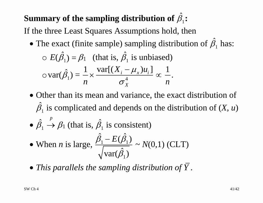
Summary of the sampling distribution of 1 :

If the three Least Squares Assumptions hold, then

• The exact (finite sample) sampling distribution of 1 has:

o E( 1 ) = 1 (that is, 1 is unbiased)

o var( 1 ) = 4

var[( ) ]1 i x i

X

X u

n

1

n.

• Other than its mean and variance, the exact distribution of

1 is complicated and depends on the distribution of (X, u)

• 1 p

1 (that is, 1 is consistent)

• When n is large, 1 1

1

ˆ ˆ( )

ˆvar( )

E

~ N(0,1) (CLT)

• This parallels the sampling distribution of Y .

SW Ch 4 42/42

We are now ready to turn to hypothesis tests & confidence

intervals…