Mathematical Tools for Data Science Spring 2021

Linear regression

1 Mean squared error estimation

1.1 Minimum mean squared error estimation

We consider the problem of estimating a certain quantity of interest that we model as a randomvariable y. We evaluate our estimate using its average squared deviation from y, which we callthe mean squared error (MSE). Imagine that the only information we have is the probabilitydistribution of y, i.e. its probability mass function (pmf) or probability density function (pdf).For example, we want to estimate the temperature in New York tomorrow, but without up-to-datemeteorological observations. We only have access to a probability distribution of temperaturesobtained from historical data. Since we have no measurements related to y, we can only generatea constant estimate using the pdf or pmf of y. In that case, the best possible estimate in terms ofMSE is the mean of y.

Theorem 1.1 (Minimum MSE constant estimate). For any random variable y with finite mean,E(y) is the best constant estimate of y in terms of MSE,

E(y) = arg minc∈R

E((c− y)2

). (1)

Proof. Let g(c) := E ((c− y)2) = c2 − 2cE (y) + E (y2), we have

g′(c) = 2(c− E(y)), (2)

g′′(c) = 2. (3)

The function is strictly convex and has a minimum where the derivative equals zero, i.e. when cis equal to the mean.

Now let us study a more interesting situation where we do have some data related to our quantityof interest, which we call the response (or dependent variable). We model these quantities, whichwe call the features (also known as covariates or independent variables) as a random vector xbelonging to the same probability space as y. In our temperature example, these features couldbe the humidity, wind speed, temperature at other locations, etc. Estimating the response fromthe features is a fundamental problem in statistics known as regression.

If we observe that x equals a fixed value x, the uncertainty about y is captured by the distributionof y given x = x. Let w be a random variable that follows that distribution. Minimizing theMSE for the fixed observation x = x is exactly equivalent to finding a constant vector c thatminimizes E[(w− c)2]. By Theorem 1.1 the optimal estimator is the mean of the distribution, i.e.the conditional mean E(y | x = x). Recall that in statistics an estimator is a function of the datathat provides an estimate of our quantity of interest. The following theorem shows that this isindeed the optimal estimator in terms of MSE. The proof is identical to that of Theorem 1.1.

Carlos Fernandez-Granda, Courant Institute of Mathematical Sciences and Center for Data Science, NYU

1

0 5 10 15 20 25Maximum temperature

0255075

100125150175200

Rain

Nonlinear regressionLinear regression

0 5 10 15 20 25Maximum temperature

5

0

5

10

15

Min

imum

tem

pera

ture

Nonlinear regressionLinear regression

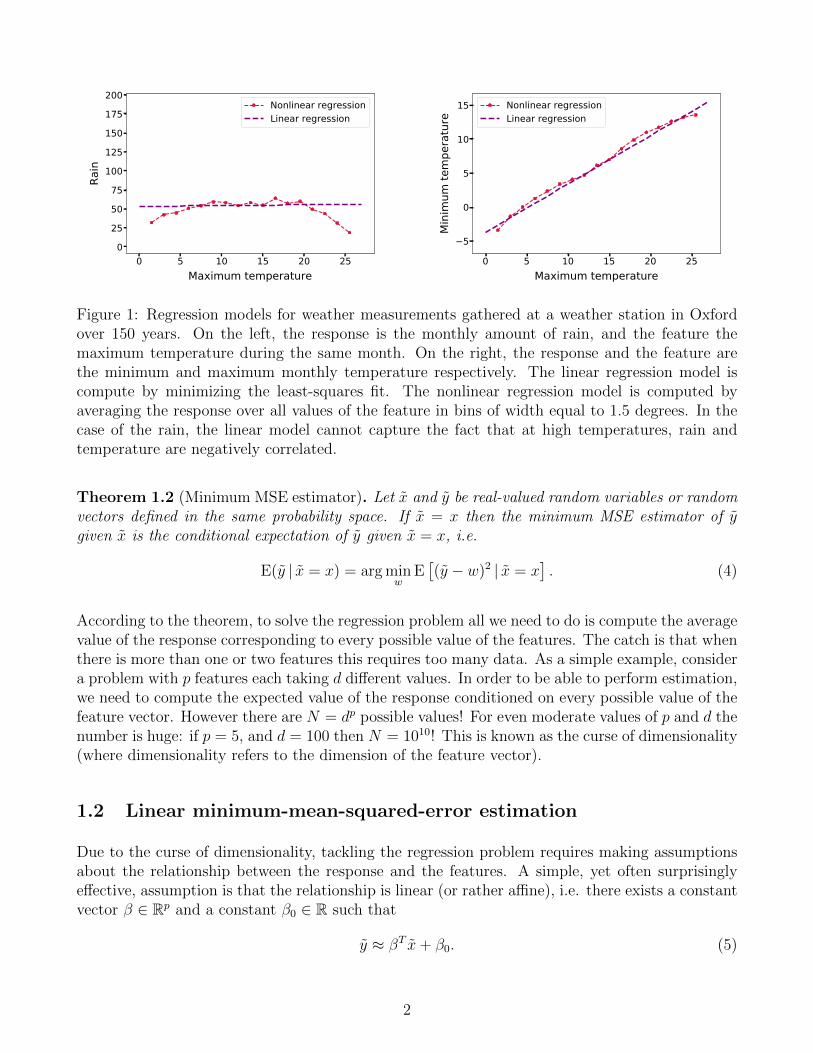
Figure 1: Regression models for weather measurements gathered at a weather station in Oxfordover 150 years. On the left, the response is the monthly amount of rain, and the feature themaximum temperature during the same month. On the right, the response and the feature arethe minimum and maximum monthly temperature respectively. The linear regression model iscompute by minimizing the least-squares fit. The nonlinear regression model is computed byaveraging the response over all values of the feature in bins of width equal to 1.5 degrees. In thecase of the rain, the linear model cannot capture the fact that at high temperatures, rain andtemperature are negatively correlated.

Theorem 1.2 (Minimum MSE estimator). Let x and y be real-valued random variables or randomvectors defined in the same probability space. If x = x then the minimum MSE estimator of ygiven x is the conditional expectation of y given x = x, i.e.

E(y | x = x) = arg minw

E[(y − w)2 | x = x

]. (4)

According to the theorem, to solve the regression problem all we need to do is compute the averagevalue of the response corresponding to every possible value of the features. The catch is that whenthere is more than one or two features this requires too many data. As a simple example, considera problem with p features each taking d different values. In order to be able to perform estimation,we need to compute the expected value of the response conditioned on every possible value of thefeature vector. However there are N = dp possible values! For even moderate values of p and d thenumber is huge: if p = 5, and d = 100 then N = 1010! This is known as the curse of dimensionality(where dimensionality refers to the dimension of the feature vector).

1.2 Linear minimum-mean-squared-error estimation

Due to the curse of dimensionality, tackling the regression problem requires making assumptionsabout the relationship between the response and the features. A simple, yet often surprisinglyeffective, assumption is that the relationship is linear (or rather affine), i.e. there exists a constantvector β ∈ Rp and a constant β0 ∈ R such that

y ≈ βT x+ β0. (5)

2

Mathematically, the gradient of the regression function is constant, which means that the rate ofchange in the response with respect to the features does not depend on the feature values. Thisis illustrated in Figure 1, which compares a linear model with a nonlinear model for two simpleexamples where there is only one feature. The slope of the nonlinear estimate varies dependingon the feature, but the slope of the linear model is constrained to be constant.

The following lemma establishes that when fitting an affine model by minimizing MSE, we canjust center the response and the features, and fit a linear model without additive constants.

Lemma 1.3 (Centering works). For any β ∈ Rp and any random variable y and p-dimensionalrandom vector x,

minβ0

E[(y − xTβ − β0)2

]= E

[(c(y)− c(x)Tβ)2

], (6)

where c(y) := y − E(y) and c(x) := x− E(x).

Proof. By Theorem 1.1, if we just optimize over β0 the minimum is E(y − xTβ), so

minβ0

E[(y − xTβ − β0)2

]= E

[(y − xTβ − E(y) + E(x)Tβ)2

](7)

= E[(c(y)− βT c(x))2

]. (8)

From now on, we will assume that the response and the features are centered. The followingtheorem derives the linear estimator that minimizes MSE. Perhaps surprisingly, it only dependson the covariance matrix of the features and the cross-covariance between the response and thefeatures.

Theorem 1.4 (Linear minimum MSE estimator). Let y be a zero-mean random variable and x azero mean random vector with a full-rank covariance matrix equal to Σx, then

Σ−1x Σxy = arg minβ

E[(y − xTβ)2

], (9)

where Σxy is the cross-covariance between x and y:

Σxy[i] := E (x[i]y) , 1 ≤ i ≤ p. (10)

The MSE of this estimator equals Var(y)− ΣTxyΣ

−1x Σxy.

Proof. We have

E((y − xTβ)2) = E(y2)− 2E (yx)T β + βTE(xxT )β (11)

= βTΣxβ − 2ΣTxyβ + Var (y) := f(β). (12)

The function f is a quadratic form. Its gradient and Hessian equal

∇f(β) = 2Σxβ − 2Σxy, (13)

∇2f(β) = 2Σx. (14)

The data are available here.

3

Covariance matrices are positive semidefinite. For any vector v ∈ Rp

vTΣxv = Var(vT x

)≥ 0. (15)

Since Σx is full rank, it is actually positive definite, i.e. the inequality is strict as long as v 6= 0.This means that the quadratic function is strictly convex and we can set its gradient to zero tofind its unique minimum. For the sake of completeness, we provide a simple proof of this. Thequadratic form is exactly equal to its second-order Taylor expansion around any point β1 ∈ Rp.For all β2 ∈ Rp

f(β2) =1

2(β2 − β1)T∇2f(β1)(β2 − β1) +∇f(β1)

T (β2 − β1) + f(β1). (16)

The equality can be verified by expanding the expression. This means that if ∇f(β∗) = 0 thenfor any β 6= β∗

f(β) =1

2(β − β∗)T∇2f(β∗)(β − β∗) + f(β∗) > f(β∗) (17)

because ∇2f(β∗) = Σx is positive definite. The unique minimum can therefore be found by settingthe gradient to zero. Finally, the corresponding MSE equals

E[(y − xTΣ−1x Σxy)

2]

= E(y2) + ΣTxyΣ

−1x E(xxT )Σ−1x Σxy − 2E(yxT )Σ−1x Σxy

= Var(y)− ΣTxyΣ

−1x Σxy. (18)

Example 1.5 (Noise cancellation). We are interested in recording the voice of a pilot in a heli-copter. To this end we place a microphone inside his helmet and another microphone outside. Wemodel the measurements as

x[1] = y + αz (19)

x[2] = αy + z, (20)

where y is a random variable modeling the voice of the pilot, z is a random variable modelingthe noise in the helicopter, and 0 < α < 1 is a constant that models the effect of the helmet.From past data, we determine that y, and z are zero mean and uncorrelated with each other. Thevariances of y and z are equal to 1 and 100 respectively.

By independence

Var(x[1]) = 1 + 100α2, (21)

Var(x[2]) = α2Var(y) + Var(z) (22)

= α2 + 100, (23)

Cov(x[1]x[2]) = αE(y2) + αE(z2) (24)

= 101α, (25)

Cov(yx[1]) = 1, (26)

Cov(yx[2]) = α, (27)

(28)

4

so

Σx =

[1 + 100α2 101α

101α α2 + 100

], (29)

Σbx =

[1α

], (30)

and by Theorem 1.4 the estimator equals

y(x) = xT[1 + 100α2 101α

101α α2 + 100

]−1 [1α

](31)

= xT1

(1 + 100α2)(α2 + 100)− 1012α2

[α2 + 100 −101α−101α 1 + 100α2

] [1α

](32)

= xT1

100(1− α2)2

[100(1− α2)−100α(1− α2)

](33)

=x[1]− αx[2]

1− α2. (34)

Notice that

y(x) =x[1]− αx[2]

1− α2(35)

=y + αz − α(αy + z)

1− α2(36)

= y (37)

so the estimate is perfect! The linear estimator cancels out the noise completely by scaling thesecond measurement and subtracting it from the first one. 4

1.3 Additive data model

In this section we analyze the linear minimum MSE estimator under the assumption that the dataare indeed generated by a linear model. To account for model inaccuracy and noise we incorporatean additive scalar z. More precisely, we assume that the response equals

y = xTβtrue + z., (38)

where βtrue ∈ Rp is a vector of true linear coefficients βtrue ∈ Rp. A common assumption isthat the noise z and the features are independent. In that case, the MSE achieved by the linearminimum MSE estimator is equal to the variance of the noise. This make sense, because the noiseis unpredictable as it is independent from the observed features.

Theorem 1.6 (Linear minimum MSE for additive model). Let x and z in Eq. (38) be zero meanand independent. Then the MSE achieved by the linear minimum MSE estimator of y given x isequal to the variance of z.

5

Proof. By independence of x and z, and linearity of expectation we have

Var(y) = Var(xTβtrue + z) (39)

= βTtrueE(xxT

)βtrue + Var (z) (40)

= βTtrueΣxβtrue + Var (z) , (41)

Σxy = E(x(xTβtrue + z)

)(42)

= Σxβtrue. (43)

By Theorem 1.2,

MSE = Var(y)− ΣTxyΣ

−1x Σxy (44)

= βTtrueΣxβtrue + Var(z)− βTtrueΣxΣ−1x Σxβtrue (45)

= Var(z). (46)

2 Ordinary least squares

In Section 1 we have studied the regression problem under the idealized assumption that we haveaccess to the true joint statistics (covariance and cross-covariance) of the response and the features.In practice, we need to perform estimation based on a finite set of data. Assume that we haveavailable n examples consisting of feature vectors coupled with their respective response: (y1, x1),(y2, x2), . . . , (yn, xn), where yi ∈ R and xi ∈ Rp for 1 ≤ i ≤ n. We define a response vector y ∈ Rn,such that y[i] := yi, and a feature matrix X ∈ Rp×n with columns equal to the feature vectors,

X :=[x1 x2 · · · xn

]. (47)

If we interpret the feature data as samples of x and the corresponding response values as samplesof y, a reasonable estimate for the covariance matrix is the sample covariance matrix,

1

nXXT =

1

n

n∑i=1

xixTi . (48)

Similarly, the cross-covariance can be approximated by the sample cross-covariance, which containsthe sample covariance between each feature and the response,

1

nXy =

1n

∑ni=1 xi[1]yi

1n

∑ni=1 xi[2]yi

· · ·1n

∑ni=1 xi[p]yi

. (49)

We obtain the following approximation to the linear minimum MSE estimator derived in Theo-rem 1.4,

Σ−1x Σxy ≈ (XXT )−1Xy. (50)

6

This estimator has an alternative interpretation, which does not require probabilistic assumptions:it minimizes the least-squares fit between the observed values of the response and the linear model.In the statistics literature, this method is known as ordinary least squares (OLS).

Theorem 2.1 (Ordinary least squares). If X :=[x1 x2 · · · xn

]∈ Rp×n is full rank and n ≥ p,

for any y ∈ Rn we have

βOLS := arg minβ

n∑i=1

(yi − xTi β

)2(51)

= (XXT )−1Xy. (52)

Proof.

n∑i=1

(yi − xTi β

)2= ‖y −XTβ‖22 (53)

= βTXXTβ − 2yTXTβ + yTy := f(β). (54)

The function f is a quadratic form. Its gradient and Hessian equal

∇f(β) = 2XXTβ − 2Xy, (55)

∇2f(β) = 2XXT . (56)

Since X is full rank, XXT is positive definite because for any nonzero vector v

vTXXTv =∣∣∣∣XTv

∣∣∣∣22> 0. (57)

By the same argument in Theorem 1.4, the unique minimum can be found by setting the gradientto zero.

In practice, large-scale least-squares problems are not solved by using the closed-form solution,due to the computational cost of inverting the sample covariance matrix of the features, but ratherby applying iterative optimization methods such as conjugate gradients.

Example 2.2 (Temperature prediction via linear regression). We consider a dataset of hourlytemperatures measured at weather stations all over the United States. Our goal is to design amodel that can be used to estimate the temperature in Yosemite Valley from the temperaturesof 133 other stations, in case the sensor in Yosemite fails. We perform estimation by fitting alinear model where the response is the temperature in Yosemite and the features are the rest ofthe temperatures (p = 133). We use 103 measurements from 2015 as a test set, and train a linearmodel using a variable number of training data also from 2015 but disjoint from the test data. Inaddition, we test the linear model on data from 2016. Figure 2 shows the results. With enoughdata, the linear model achieves an error of roughly 2.5°C on the test data, and 2.8°C on the 2016data. The linear model outperforms a naive single-station estimate, which uses the station thatbest predicts the temperature in Yosemite for the training data. 4The data are available at http://www1.ncdc.noaa.gov/pub/data/uscrn/products

7

200 500 1000 2000 5000Number of training data

0

1

2

3

4

5

6

7

Aver

age

erro

r (de

g Ce

lsius

)

Training errorTest errorTest error (2016)Test error (single-station estimate)

Figure 2: Performance of the OLS estimator on the temperature data described in Example 2.2.The graph shows the square root of the MSE (RMSE) achieved by the model on the training andtest sets, and on the 2016 data, for different number of training data and compares it to the RMSEof the best single-station estimate.

3 The singular-value decomposition

In order to gain further insight into linear models we introduce a fundamental tool in linearalgebra: the singular-value decomposition. We omit the proof of its existence, which follows fromthe spectral theorem for symmetric matrices.

Theorem 3.1 (Singular-value decomposition). Every real matrix A ∈ Rm×k, m ≥ k, has asingular-value decomposition (SVD) of the form

A =[u1 u2 · · · uk

]s1 0 · · · 00 s2 · · · 0

. . .

0 0 · · · sk

[v1 v2 · · · vk]T

(58)

= USV T , (59)

where the singular values s1 ≥ s2 ≥ · · · ≥ sk are nonnegative real numbers, the left singular vectorsu1, u2, . . .uk ∈ Rm form an orthonormal set, and the right singular vectors v1, v2, . . . vk ∈ Rk

also form an orthonormal set.

8

If m < k then the SVD is of the form

A =[u1 u2 · · · um

]s1 0 · · · 00 s2 · · · 0

. . .

0 0 · · · sm

[v1 v2 · · · vm]T

(60)

= USV T , (61)

where s1 ≥ s2 ≥ · · · ≥ sm are nonnegative real numbers, and the singular vectors u1, u2, . . .um ∈Rm, and v1, v2, . . . vm ∈ Rk form orthonormal sets.

The SVD provides a very intuitive geometric interpretation of the action of a matrix A ∈ Rm×k

on a vector w ∈ Rk, as illustrated in Figure 3:

1. Rotation of w to align the component of w in the direction of the ith right singular vectorvi with the ith axis:

V Tw =k∑i=1

〈vi, w〉ei, (62)

where ei is the ith standard basis vector.

2. Scaling of each axis by the corresponding singular value

SV Tw =k∑i=1

si〈vi, w〉ei. (63)

3. Rotation to align the ith axis with the ith left singular vector

USV Tw =k∑i=1

si〈vi, w〉ui. (64)

Another consequence of the spectral theorem for symmetric matrices is that the maximum scalingproduced by a matrix is equal to the maximum singular value. The maximum is achieved whenthe matrix is applied to any vector in the direction of the right singular vector v1. If we restrict ourattention to the orthogonal complement of v1, then the maximum scaling is the second singularvalue, due to the orthogonality of the singular vectors. In general, the direction of maximumscaling orthogonal to the first i − 1 left singular vectors is equal to the ith singular value andoccurs in the direction of the ith singular vector.

Theorem 3.2. For any matrix A ∈ Rm×k, the singular values satisfy

s1 = max{‖w‖2=1 | w∈Rk}

‖Aw‖2, (65)

si = max{‖w‖2=1 | w∈Rk, w⊥v1,...,vi−1}

‖Aw‖2, (66)

(67)

9

(a) s1 = 3, s2 = 1.

~x

~v1

~v2

~y

V T~x

~e1

~e2V T~y

SV T~x

s1~e1

s2~e2SV T~y

USV T~x

s1~u1s2~u2

USV T~y

V T

S

U

(b) s1 = 3, s2 = 0.

~x

~v1

~v2

~y

V T~x

~e1

~e2V T~y

SV T~xs1~e1

~0 SV T~y

USV T~x

s1~u1

~0

USV T~y

V T

S

U

Figure 3: The action of any matrix can be decomposed into three steps: rotation to align theright singular vectors to the axes, scaling by the singular values and a final rotation to align theaxes with the left singular vectors. In image (b) the second singular value is zero, so the matrixprojects two-dimensional vectors onto a one-dimensional subspace.

10

and the right singular vectors satisfy

v1 = arg max{‖w‖2=1 | w∈Rk}

‖Aw‖2, (68)

vi = arg max{‖w‖2=1 | w∈Rk, w⊥v1,...,vi−1}

‖Aw‖2, 2 ≤ i ≤ k. (69)

The SVD provides a geometric interpretation of the OLS estimator derived in Theorem 2.1. LetX = USV T be the SVD of the feature matrix, then

βOLS =(XXT

)−1Xy (70)

= (US2UT )−1USV Ty (71)

= US−2UTUSV Ty (72)

= US−1V Ty. (73)

The OLS estimator is obtained by inverting the action of the feature matrix. This is achieved bycomputing the components of the response vector in the direction of the right singular vectors,scaling by the inverse of the corresponding singular values, and then rotating so that each com-

ponent is aligned with the corresponding left singular vector. The matrix(XXT

)−1X is called a

left inverse or pseudoinverse of XT because(XXT

)−1XXT = I.

4 Analysis of ordinary-least-squares estimation

In order to study the properties of OLS, we study an additive model. The training data are equalto the n-dimensional vector

ytrain := XTβtrue + ztrain, (74)

where X ∈ Rp×n contains n p-dimensional feature vectors. The noise ztrain is modeled as an n-dimensional iid Gaussian vector with zero mean and variance σ2. The feature matrix X is fixedand deterministic. OLS is equivalent to maximum-likelihood estimation under this model.

Lemma 4.1. If the training data are interpreted as a realization of the random vector in Eq. (74)the maximum-likelihood estimate of the coefficients is equal to the OLS estimator.

Proof. The likelihood is the probability density function of ytrain evaluated at the observed dataytrain and interpreted as a function of the coefficient vector β,

Lytrain(β) =1√

(2πσ2)nexp

(− 1

2σ2

∣∣∣∣ytrain −XTβ∣∣∣∣22

). (75)

The maximum-likelihood estimate equals

βML = arg maxβLytrain(β) (76)

= arg maxβ

logLytrain(β) (77)

= arg minβ

∣∣∣∣ytrain −XTβ∣∣∣∣22. (78)

11

(β − βtrue)TXXT (β − βtrue) (β − βtrue)TXXT (β − βtrue) = 0.1

−3 −2 −1 0 1 2 3 4 5 6

β[2]

−2

−1

0

1

2

3

4

β[1] βtrue

0.25

0.50

0.50

1.00

1.00

2.00

2.00

4.00

4.00

7.00

7.00

0.10

−3 −2 −1 0 1 2 3 4 5 6

β[2]

−2

−1

0

1

2

3

4

β[1]

c s−11 u1

c s−12 u2βtrue

0.10

Figure 4: Deterministic quadratic component of the least-squares cost function (see Eq. (80))for an example with two features where the left singular vectors of X align with the horizontaland vertical axes, and the singular values equal 1 and 0.1. The quadratic form is an ellipsoidcentered at βtrue with axes aligned with the left singular vectors. The curvature of the quadraticis proportional to the square of the singular values.

In the following sections we analyze the OLS coefficient estimate, as well as its correspondingtraining and test errors when the training data follow the additive model.

4.1 Analysis of OLS coefficients

If the data follow the additive model in (74), the OLS cost function can be decomposed into adeterministic quadratic form centered at βtrue and a random linear function that depends on thenoise,

arg minβ‖ytrain −XTβ‖22 = arg min

β‖ztrain −XT (β − βtrue)‖22 (79)

= arg minβ

(β − βtrue)TXXT (β − βtrue)− 2zTtrainXT (β − βtrue) + zTtrainztrain

= arg minβ

(β − βtrue)TXXT (β − βtrue)− 2zTtrainXTβ. (80)

Figure 4 shows the quadratic component for a simple example with two features. Let X = USV T

be the SVD of the feature matrix. The contour lines of the quadratic form are ellipsoids, definedby the equation

(β − βtrue)TXXT (β − βtrue) = (β − βtrue)TUS2UT (β − βtrue) (81)

=

p∑i=1

s2i (uTi (β − βtrue))2 = c2 (82)

for a constant c. The axes of the ellipsoid are the left singular vectors of X. The curvature inthose directions is proportional to the square of the singular values, as shown in Figure 4. Due

12

−2zTtrainXTβ (β − βtrue)TXXT (β − βtrue)− 2zTtrainX

Tβ

−3 −2 −1 0 1 2 3 4 5 6

β[2]

−2

−1

0

1

2

3

4

β[1]

-0.20

-0.00

0.20

0.40

−3 −2 −1 0 1 2 3 4 5 6

β[2]

−2

−1

0

1

2

3

4

β[1]βOLSβtrue

0.250.50

0.50

1.00

1.00

2.00

2.00

4.00

4.00

7.00

7.00

−3 −2 −1 0 1 2 3 4 5 6

β[2]

−2

−1

0

1

2

3

4

β[1]

-0.60

-0.40

-0.20

-0.000.20

0.40

0.60 0.80

1.00

1.20

1.40

−3 −2 −1 0 1 2 3 4 5 6

β[2]

−2

−1

0

1

2

3

4

β[1]βOLS βtrue

0.50

1.00

1.00

2.00

2.00

4.00

4.00

7.00

7.00

10.00

Figure 5: The left column show two realizations of the random linear component of the least-squares cost function (see Eq. (80)) for the example in Figure 4. The right column shows thecorresponding cost function, which is a quadratic centered at a point that does not coincide withβtrue due to the linear term. The minimum of the quadratic is denoted by βOLS.

to the random linear component, the minimum of the least-squares cost function is not at βtrue.Figure 4 shows this for a simple example. The following theorem shows that the minimum of thecost function is a Gaussian random vector centered at βtrue.

Theorem 4.2. If the training data follow the additive model in Eq. (74) and X is full rank, theOLS coefficient

βOLS := arg minβ

∣∣∣∣ytrain −XTβ∣∣∣∣2, (83)

is a Gaussian random vector with mean βtrue and covariance matrix σ2US−2UT , where X = USV T

is the SVD of the feature matrix.

13

−3 −2 −1 0 1 2 3 4 5 6

β[2]

−2

−1

0

1

2

3

4

β[1]

βtrue

βOLS

−3 −2 −1 0 1 2 3 4 5 6

β[2]

−2

−1

0

1

2

3

4

β[1]

c s−11 u1

c s−12 u2βtrue

10−15

10−13

10−11

10−9

10−7

10−5

10−3

10−1

Figure 6: The left image is a scatterplot of OLS estimates corresponding to different noise re-alizations for the example in Figure 5. The right image is a heatmap of the distribution of theOLS estimate, which is centered at βtrue and has covariance matrix σ2US−2UT , as established inTheorem 4.2.

Proof. We have

βOLS = (XXT )−1Xytrain (84)

= (XXT )−1XXTβtrue + (XXT )−1Xztrain (85)

= βtrue + (XXT )−1Xztrain (86)

= βtrue + US−1V T ztrain. (87)

The result then follows from Theorem 3.4 in the lecture notes on the covariance matrix.

Figure 6 shows a scatterplot of the OLS estimates corresponding to different noise realizations, aswell as the distribution of the OLS estimate. The contour lines of the distribution are ellipsoidalwith axes aligned with the left singular vectors of the feature matrix. The variance along thoseaxes is proportional to the inverse of the squared singular values. If there are singular values thatare very small, the variance in the direction of the corresponding singular vector can be very large,as is the case along the horizontal axis of Figure 6.

4.2 Training error

In order to analyze the training error of the OLS estimator, we leverage a geometric perspective.The OLS estimator approximates the response vector y using a linear combination of the corre-sponding features. Each feature corresponds to a row of X. The linear coefficients weight theserows. This means that the estimator is equal to the vector in the row space of the feature matrixX that is closest to y. By definition, that vector is the orthogonal projection of y onto row(X).Figure 7 illustrates this with a simple example with two features and three examples.

Lemma 4.3. Let X ∈ Rp×n be full-rank feature matrix, where n ≥ p, and let y ∈ Rn be a response

14

Figure 7: Illustration of Lemma 4.3 for a problem with two features corresponding to the two rowsof the feature matrix X1: and X2:. The least-squares solution is the orthogonal projection of thedata onto the subspace spanned by these vectors.

vector. The OLS estimator XTβOLS of y given X, where

βOLS := arg minβ∈Rp

∣∣∣∣y −XTβ∣∣∣∣2, (88)

is equal to the orthogonal projection of y onto the row space of X.

Proof. Let USV T be the SVD of X. By Eq. (73)

XTβOLS = XTUS−1V Ty (89)

= V SUTUS−1V Ty (90)

= V V Ty. (91)

Since the rows of V form an orthonormal basis for the row space of X the proof is complete.

The result provides an intuitive interpretation for the training error achieved by OLS for theadditive model in Eq. (74): it is the projection of the noise vector onto the subspace spanned bythe feature vectors.

Lemma 4.4. If the training data follow the additive model in Eq. (74) and X is full rank, thetraining error of the OLS estimator XT βOLS is the projection of the noise onto the orthogonalcomplement of the row space of X.

15

Proof. By Lemma 4.3

ytrain −XT βOLS = ytrain − Prow(X) ytrain (92)

= XTβtrue + ztrain − Prow(X) (XTβtrue + ztrain) (93)

= XTβtrue + ztrain −XTβtrue − Prow(X) ztrain (94)

= Prow(X)⊥ ztrain. (95)

We define the average training square error as the average error incurred by the OLS estimatoron the training data,

E2train :=

1

n

∣∣∣∣∣∣ytrain −XT βOLS

∣∣∣∣∣∣22. (96)

By Lemma 4.4, if the noise is Gaussian, then the training error is the projection of an n-dimensionaliid Gaussian random vector onto the subspace orthogonal to the span of the feature vectors. Theiid assumption means that the Gaussian distribution is isotropic. The dimension of this subspaceequals n − p, so the fraction of the variance in the Gaussian vector that lands on it should beapproximately equal to 1− p/n. The following theorem establishes that this is indeed the case.

Theorem 4.5. If the training data follow the additive model in Eq. (74) and X is full rank, thenthe mean of the average training error defined in Eq. (96) equals

E(E2

train

)= σ2

(1− p

n

)(97)

and its variance equals

Var(E2train) =

2σ4(n− p)n2

. (98)

Proof. By Lemma 4.4

nE2train =

∣∣∣∣Prow(X)⊥ ztrain∣∣∣∣22

(99)

= zTtrainV⊥VT⊥ V⊥V

T⊥ ztrain (100)

=∣∣∣∣V T⊥ ztrain

∣∣∣∣22, (101)

where the columns of V⊥ are an orthonormal basis for row(X)⊥. V T⊥ ztrain is a Gaussian vector of

dimension n− p with covariance matrix

ΣV T⊥ ztrain

= V T⊥ ΣztrainV⊥ (102)

= V T⊥ σ

2IV⊥ (103)

= σ2I. (104)

The error is therefore equal to the square `2 norm of an iid Gaussian random vector. Let w be ad-dimensional zero-mean Gaussian random vector w with unit variance. The expected value of its

16

square `2 norm is

E(||w||22

)= E

(d∑i=1

w[i]2

)(105)

=d∑i=1

E(w[i]2

)(106)

= d. (107)

The mean square equals

E[(||w||22

)2]= E

( d∑i=1

w[i]2

)2 (108)

=d∑i=1

d∑j=1

E(w[i]2w[j]2

)(109)

=d∑i=1

E(w[i]4

)+ 2

d−1∑i=1

d∑j=i+1

E(w[i]2

)E(w[j]2

)(110)

= 3d+ d(d− 1) (the 4th moment of a standard Gaussian equals 3) (111)

= d(d+ 2), (112)

so the variance equals

Var(||w||22

)= E

[(||w||22

)2]− E2(||w||22

)(113)

= 2d. (114)

As d grows, the relative deviation of the squared norm of the Gaussian vector from its meandecreases proportionally to

√2/d, as shown in Figure 8. Geometrically, the probability density

concentrates close to the surface of a sphere with radius√d. By definition of the training error,

we have

E2train =

1

n

∣∣∣∣V T⊥ ztrain

∣∣∣∣22

(115)

=σ2

n||w||22 , (116)

so the result follows from setting d := n− p in Eqs. (107) and (114).

The variance of the square error scales with 1/n, which implies that the error concentrates aroundits mean with high probability as the number of examples in the training set grows.

For large n, the error equals the variance of the noisy component σ2, which is the error achieved bythe true coefficients βtrue. When n ≈ p, however, the error can be much smaller. This is bad news.We cannot possibly fit the noisy component of the response using the features, because they are

17

101 102 103

Dimension

100

101

2 nor

m o

f sam

ples

Dimension

Figure 8: The graphs shows the `2 norm of 100 independent samples from standard Gaussianrandom vectors in different dimensions. The norms of the samples concentrate around the squareroot of the dimension.

independent. Therefore, if an estimator achieves an error of less than σ it must be overfitting thetraining noise, which will result in a higher generalization error on held-out data. This suggeststhat the OLS estimator overfits the training data when the number of examples is small withrespect to the number of features. Figure 9 shows that this is indeed the case for the dataset inExample 2.2. In fact, the training error is proportional to

(1− p

n

)as predicted by our theoretical

result.

4.3 Test error

The test error of an estimator quantifies its performance on held-out data, which have not beenused to fit the model. We model the test data as

ytest := xTtestβtrue + ztest. (117)

The linear coefficients are the same as in the training set, but the features and noise are different.The features are modeled as a p-dimensional random vector xtest with zero mean (the featuresare assumed to be centered) and the noise ztest is a zero-mean Gaussian random variable with thesame variance σ2 as the training noise. The training and test noise are assumed to be independentfrom each other and from the features. Our goal is to characterize the test error

Etest := ytest − xTtestβOLS (118)

= ztest + xTtest

(βtrue − βOLS

), (119)

where βOLS is computed from the training data.

Theorem 4.6 (Test mean square error). If the training data follow the additive model in Eq. (74),X is full rank, and the test data follow the model in Eq. (117), then the mean square of the test

18

error equals

E(E2test) = σ2

(1 +

p∑i=1

Var(uTi xtest)

s2i

), (120)

where Σxtest is the covariance matrix of the feature vector, s1, . . . , sp are the singular values of Xand v1, . . . , vp are the right singular vectors.

Proof. By assumption, the two components of the test error in Eq. (119) are independent, so thevariance of their sum is the sum of their variances:

Var(ytest − xTtestβOLS

)= σ2 + Var

(xTtest

(βtrue − βOLS

))(121)

Since everything is zero mean, this also holds for the mean square. Let USV T be the SVD of X.The coefficient error equals

βOLS − βtrue =

p∑i=1

vTi ztrainsi

ui, (122)

by Theorem 4.2. This implies

E

[(xTtest

(βtrue − βOLS

))2]= E

( p∑i=1

vTi ztrain uTi xtest

si

)2 (123)

=

p∑i=1

E[(vTi ztrain)2

]E[(uTi xtest)

2]

s2i, (124)

where the second equality holds because when we expand the square, the cross terms cancel dueto the independence assumptions and linearity of expectation. For i 6= j

E

(vTi ztrain u

Ti xtest

si

vTj ztrain uTj xtest

sj

)=

E(uTi xtestu

Tj xtest

)sisj

vTi E(ztrainz

Ttrain

)vj (125)

=E(uTi xtestu

Tj xtest

)sisj

vTi vj (126)

= 0. (127)

By linearity of expectation, we conclude

E

[(xTtest

(βtrue − βOLS

))2]=

p∑i=1

vTi E(ztrainzTtrain)viu

Ti E(xtestx

Ttest)ui

s2i(128)

= σ2

p∑i=1

uTi Σxtestuis2i

, (129)

because the covariance matrix of the training noise ztrain equals σ2I.

19

200 500 1000 2000 5000Number of training data

0

1

2

3

4

5

6

7

Aver

age

erro

r (de

g Ce

lsius

)

1 p/n1 + p/n

Training errorTest error

Figure 9: Comparison of the theoretical approximation for the training and test error of the OLSwith the actual errors on the temperature data described in Example 2.2. The parameter σ isfixed based on the asymptotic value of the error.

The square of the ith singular value of the training covariance matrix is proportional to the samplevariance of the training data in the direction of the ith singular value ui,

s2in

=uiXX

Tuin

(130)

= uTi ΣXui (131)

= var (Pui X ) . (132)

If this sample variance is a good approximation to the variance of the test data in that directionthen

E(E2test) ≈ σ2

(1 +

p

n

). (133)

However, if the training data is not large enough, the sample covariance matrix of the trainingdata may not provide a good estimate of the feature variance in every direction. In that case, theremay be terms in the test error where si is very small, due to correlations between the features,but the true directional variance is not. Figure 10 shows that some of the singular values of thetraining matrix in the temperature prediction are indeed minuscule. Unless the test variance inthat direction cancel them out, this results in a large test error.

Intuitively, estimating the contribution of low-variance components of the feature vector to thelinear coefficients requires amplifying them. This also amplifies the training noise in those direc-tions. When estimating the response, this amplification is neutralized by the corresponding smalldirectional variance of the test features as long as it occurs in the right directions (which is thecase if the sample covariance matrix is a good approximation to the test covariance matrix). Oth-erwise, it will result in a high response error. This typically occurs when the number of training

20

200 500 1000 2000 5000Number of training data

10 3

10 2

10 1

100

101

Sing

ular

val

ues o

f tra

inin

g m

atrix

Figure 10: Singular values of the training matrix in Example 2.2 for different numbers of trainingdata.

data is small with respect to the number of features. The effect is apparent in Figure 2 for smallvalues of n.

21