Linear programming via a quadratic penalty...

Mathematical Methods of Operations Research (1996)44:345-370

Linear Programming via a Quadratic Penalty Function 1

MUSTAFA ~. P I N ~

IE Department, Bilkent University, 06533 Bilkent, Ankara, Turkey

Abstract: We use quadratic penalty functions along with some recent ideas from linear 11 estimation to arrive at a new characterization of primal optimal solutions in linear programs. The algorithmic implications of this analysis are studied, and a new, finite penalty algorithm for linear programming is designed. Preliminary computational results are presented.

Key Words: Quadratic Penalty Functions. Linear Programming. Linear 11 Estimation. Characteri- zation. Finite Algorithms.

1 Introduction

W e cons ide r the p r i m a l l inear p r o g r a m m i n g p r o b l e m

FP] m i n i m i z e cTx X

subject to A x = b

x > 0

where x ~ 9~", A is a m x n mat r ix , b E ~tl" a n d c ~ ~l", a n d its dual :

[D] maximize - b r y

Y

subject to ATy -t- c >_ 0

where y ~ 9W.

1 Research supported by grant No. 11-0505 from the Danish Natural Science Research Council SNF.

1432- 2994/96/44: 3/345-370 $2.50 �9 1996 Physica-Verlag, Heidelberg

346 M.~.Pinar

The first purpose of this paper is to give a new characterization of optimal solutions to a linear program using quadratic penalty functions and some recent ideas from linear 11 estimation. The second purpose is to investigate the algorithmic implications of this result for linear programming. Consider the following piecewise quadratic functional:

F(x, t) =- tc~:x + �89 + �89 , (1)

where r(x) = A x - b, t is a positive scalar and O(x) is a diagonal matrix with diagonal entries Ou:

O,(x) = {10 ifxi < 0 otherwise , (2)

and the unconstrained minimization problem:

[CP] min F(x, t) (3) XE ~ n

for decreasing positive values of t. Let xt denote a minimizer of F(x, t). It is well-known [-4] that

lim cTxt = f * , (4) t -*O

where f * is optimal value in [P]. In the present paper we characterize the solution set of [CP] and show that

an optimal solution of the linear program can be obtained by following any one of the infinitely many piecewise linear paths that lead to the solution set of [P]. This leads to a characterization of the solution set of IP]. I.e., we give a description of the solution set of I-P] using information from the minimization of the unconstrained function for sufficiently small t > 0. To the best of our knowl- edge, this is the first such result in the literature for linear programs. Following this analysis, we define a new penalty algorithm for linear programs, and analyze its finiteness. The algorithm produces infeasible primal and feasible dual iterates. The primal feasibility is obtained upon termination. A preliminary implementation and numerical results are discussed at the end of the paper. For previous work on penalty methods for linear programming see also [1, 2, 5, 11].

This analysis is made possible by adapting some recent ideas from linear 11 estimation [10]. In [10] the following problem was tackled:

[L1] min G(x) == I[Erx - dllx , (5)


where E is n x m, d e 91". In [10] a smooth approximation of [L1] was considered:

[SL1] min G~(x) - ~ p(z,(x)) , (6) i=1

where z~(x) = eirx - di,

f p(zi) = i ~ 2~

L i z~ i -~

if izil ~

otherwise .

(7)

The function p is known as the "Huber" function in robust regression [8]. Clearly, Gr is also a piecewise quadratic functional. By analyzing the behavior of the set of minimizers of G~ for decreasing values of 7, characterizations of the solutions sets of both IL l ] and [SL1] were given in [10]. It is precisely against this background that we develop our results in the present paper. Our proofs follow the same lines as in [10] with the necessary modifications. The contribu- tion of the paper is to broaden the domain of application of these recent ideas, and in the process to obtain new results on the linear programming problem. For an alternative dual approach, the reader is referred to [15].

2 Primal Pathways to Optimal Solutions

We will assume throughout the paper that A has rank m, and that A contains no row or column that is identically zero. The following result shows that the unconstrained minimization of F is well-defined.

Theorem 1: I f [P] has a finite optimal value there exists a finite point that minimizes F(x, t) for all positive t.

Proof: Assume that the conclusion is false, i.e., that there exists a sequence of points {xt} with limz-.~o IIx~ll = + o o such that l i m l ~ tcrxz = -o e . The un- boundedness of F also implies that there does not exist j ~ {1 . . . . ,m} where limt-.| Irj(xz)f = oo and there does not exist i ~ {1 . . . . , n} where limz_.o~ xi = -oo . However, this implies that [P] is unbounded since t > 0, which contra- dicts our assumption that [P] has a finite optimal value. �9

348

Define

M. (~. Pinar

~(x) = �89 + �89

The following is well-known; see e.g., [-4, 14]:

lim ~(xt) = 0 . (8) t--}O

Let us now define a binary vector 0 ~ 91" where the entries are either 0 or 1 according to the rule:

0i(x) = {~ ifxi < 0 otherwise . (9)

Hence the diagonal matrix O defined earlier in (2) can be expressed

O = diag(01 . . . . . 0.) .

In what follows Ox, and O" x are both used to denote the multiplication of a vector x with the diagonal matrix O to avoid confusion with O(x) where x is the a rgument of O. We denote by X the set of optimal solutions to [P] .

2.1 The Minimizers of F

We observe that F(x, t) is composed of a finite number of quadrat ic functions. In each domain D _c 91, where O(x) is constant F is equal to a specific quadrat ic function as seen from its definition. These domains are separated by the union of hyperplanes,

B = {x e 91"13i: x~ = 0} . (lO)

Given a point x e 9t" and the associated binary vector O(x) Qo is the quadrat ic function which equals F on the subset

rg o = cl{z ~ 91"[0(z) = O} . (11)


% corresponds to an orthant of 9~". Notice that any x e 9~"\B has exactly one corresponding orthant whereas a point x e B belongs to two or more orthant. Therefore, we must specify a binary vector 0 in addition to x in order to specify which quadratic function we are currently considering as representative of F.

Qo can be defined as follows:

Qo(z, t) = �89 - x ) r ( A r A + O)(z - x) + F ' r (x , t)(z - x) + F(x , t) . (12)

The gradient of the function F(x, t) is given by

F'(x , t) = ( A r A + O ) x -- ATb + tc . (13)

For x e 9t"'\B, the Hessian of F(x, t) exists, and is given by

F ' ( x , t) = A TA + O . (14)

The set of minimizers of F(x, t) is denoted by Mr. Now, we have the following lemma.

L e m m a 1: L e t P -~ A r A + O. Then for any x e 9t" the fo l lowing holds:

P x = O ::~ O x = O .

Proof:

x r p x = ( A x ) r ( A x ) + x r O x = llAxt]2 2 + xrOx .

Suppose

{I0 f ~ Ou = for i ~ So �9

Then, we have

{; (Ox)i = i f o r i e S 1 for i e So ,

350

and

x T O x = x ~ . i~St

Now, since []AxU2 ~ 0 and NTOx ~ 0 it follows that

P x = 0 ~ x T p x = 0 ~ A x = 0 and x T O x = 0 .

M. (~. Pinar

But

x r O x = O ~ Vi ~ S lx i = O ~ Ox = O .

Lemma 2: O(xt) is constant f o r x t ~ M t. Furthermore (xt) i is constant fo r x t e Mt

i f0 ,= 1.

Proof: Let xt ~ Mt and let 0 = O(xO, i.e., F(x , t) = Qo(x, t) for x e %. If x s % c~ M~ then Q~(x - xt) = 0. Therefore, i f(xt)i < 0 then xi - (xt)i = 0 by the previous Lemma. Thus x~ is constant in % c~ Mr. Using the fact that Mt is connected and x~ is continuous, it is easily seen by repeating the argument above that xi is c6nstant in Mr. Next suppose (xt)i >-O. Then xi >_ 0 for all x e M t because existence of x ~ M t with xi < 0 is excluded by the convexity of Mr, continuity of x~, and the first part of the lemma. This completes the proof. �9

Following the lemma we use the notation O(Mt) = O(xt), xt ~ Mt as the binary vector corresponding to the solution set. Now, Lemma 2 has the following consequences which characterize the solution set Mr.

Corollary 1: Mt is a convex set which is contained in one orthant: cg o where

0 = O(Mt).

Proof'. Follows immediately from the linearity of the problem and Lemma 2.

Corollary 2: L e t xt ~ Mt , and 0 = O(Mt). Le t ~ be the null space o f P - A r A +

O, where O = diag(01 . . . . . On). Then

M, = (x, + ~ o ) n % .


Proof: I t follows f rom (13) that F'(xt + u, t) = 0 if u e S o and xt + u e %. Thus

Mr -- (xt + ~0) n cg0 .

If x e M t then by the previous corol lary x e %. Also, F'(x, t) = 0. This implies that P(x - xt) = 0. Therefore, we have

M,~- (x t + Wo) n %

which proves the result. �9

An impor t an t consequence of the previous character izat ion of Mt is that it provides a sufficient condit ion for the uniqueness of x,.

Corollary 3: Let 0 = O(Mt). xt ~ Mt is unique if rank(Ar A + O) = n.

Notice that this condi t ion is not necessary for uniqueness of the minimizer in [CP] as the following example demonstrates:

Example 1: Consider the linear p r o g r a m of the form [P] where

A = 5 6 0 - 1

8 9 0 0

and b = (7, 5, 10) r, and c = ( - 75, - 87, - 102, 0, 5, - 8) r. Fo r t = 1, the unique minimizer o f F occurs at x t = ( - 1 , - 2 , 4, 0, 0, 5) r, where r ank (ArA + O) = 5.

2.2 Characterization of Optimal Solutions

In this section we show how the solution set M t approx imates the solution set X of [P] as t approaches 0.

Assume x, e Mr, and let 0 = O(Mt). Let X0 be defined as in Corol la ry 2.

Lemma 3: Let x t ~ Nit, and 0 = O(Mt). Then consistent,

the following linear system is

(ATA + O)d = c . (15)

352 M. (~. Pinar

P r o o f : Since x t satisfies the necessary condition for a minimizer, we have the following:

0 = ( A T A + ~9)x t - A r b + tc .

Observing that O. O = O, (16) can be rewritten as:

where 0 denotes a vector identically zero in 91". We observe that the system

(16)

(17)

(18)

is consistent since it corresponds to normal equations for the overdetermined system:

(:)h (:) ,19

Hence, the result. �9

Let d be a solution to (15). Then, it is easily verified by inserting (15) into (16) that xt + td is the least squares solution to the overdetermined system of linear equations:

(:) L e m m a 4: L e t x t e M t, and 0 = O(Mt). I f the overdetermined sys tem (19) is consis-

tent then

1 t (Ax t -- b) = - A d , (20)

and


1 - O x t = - O d (21) t

for any solution d to (15).

Proof: The proof follows by inserting the solution (x t + td) into (19). �9

Now let d solve (15) and assume O(xt + ed) = 0, i.e., xt + ed E % for some ~ > 0. The linearity of the problem implies xt + 6d ~ % for 0 < 6 < e. Therefore (16) and (15) show that (xt + 6d) is a minimizer of F(x, t - 3). Using Corollary 2 we have proved the following:

Lemma 5: Le t x t ~ M t and let 0 = O(Mt). Let d solve (15). I f O(x t + ed) = 0 for e > 0 then O(x t + 6d) = O, and

Nit_ a = (x, + 6d + Jfo)c~ % (22)

for O < a < e.

Theorem 2: There exists t o > 0 such that O(Mt) is constant for 0 < t <_ to. Furthermore,

M,_ a = (xt + 6d + ~o)c~ cg o

where 0 = O(Mt) and d solves (15).

for O _ < b < t _ < t o

Proof." Since there is only a finite number of different binary vectors the theorem is a consequence of the previous lemma. �9

The analysis shows that the minimizers of F form a family of piecewise-linear paths as a function of t.

Corollary 4: O(Mt) is a piecewise constant function o f t.

Corollary 5: Let 0 < t < t o, where t o is given in Theorem 2 and let 0 = O(Mt). Then

354 M. (~. Pinar

O.(x,+ t~)=0, (23)

and

r(x,+t~)=O, (24)

where ~t is any solution of (15). Furthermore,

{ ( A x t - b) = - A~l , (25)

and

l o x t - O~l (26) _ ~ _ _ .

t

I.e., r(xt)/t and Ox/t are constant.

Proof: Let x,_~ e Mt-~ for 0 < 6 < t. By Theorem 2 there exists d that solves (15) such that xt-~ = xt + 6d. Hence, there exists d* that solves (15) such that xt + 6d* ~ Mt-o for all 0 < 6 < t. Now, using (8)

O'(x t + td*) = 0 . (27)

Any solution d of (15) can be expressed as d = d* + ~/where r/r oA/'(ATA + 0). Now, (23) follows from (27) and Lemma 1. Using (8) we have:

r(xt + td*) = 0 . (28)

Now, (24) follows since

(ArA + O ) q = O ~ A r A q = O ~ A r l = O .

The second part follows from Lemma 4 since (23) and (24) imply that (19) is consistent. �9

We notice that if xt ~ Mt then Yt = r(xt)/t, where 0 = O(Mt), is feasible in [D] as it is seen from (16). Now we recall a classical result from linear programming known as the complementary slackness theorem; see for instance [12].


Theorem 3: Le t x ~ 9P and y ~ ~R" be feasible solutions in [P] and [D], respec-

tively. Then x and y are optimal solutions in their respective problems [P] and [D] i f and only i f the following conditions hold:

0 < x~ =. airy + ci = 0 .

a~'y + ci > 0 ~ xi = 0 .

(29)

(30)

For the purposes of our next theorem we rewrite the constraints of [D] in the form of equality constraints by introducing a non-negative vector u e tRm:

ATy -- U = --C .

Now, for xt E Mr we define

y , - - r(xt)/ t , (31)

and

ut = - O x J t (32)

where 0 = O(MO, and O is defined accordingly. Then it is easy to see that (Yt, u~) is feasible in [D] from (16).

Let Jo = {i]Oi = 0}, and ~o = {x ~ 9t"[x~ > 0 ^ i e Jo}. Now we are ready to state the new characterization of optimal solution to [P].

Theorem 4: Le t 0 < t <_ to, where t o is given in Theorem 2 and let 0 = O(Mt). Le t x t ~ Mr, and d solve (15). Then

Mo = X

where

Mo = (xt + td + Sffo) c~ ~o (33)

and

356

1 y * = ~r(x,)

solve [D].

M. ~. Pinar

u* = - l - o x t (34) t

Proof: First, Mo is non-empty as a consequence of the constant binary vector property of Theorem 2. Assume Xo e Mo. Then there exists a solution do to (15) such that x o = xt + tdo. Therefore using Corollary 5

Oxo = 0 . (35)

Furthermore, (y*, u*) is feasible for [D]. Therefore, using (24), (32), and (35) we have

crxo = x g ( - A r y * + u*)

= - x r A r y * + xgu*

= - b r y * .

Now, x o is a non-negative vector following (35) and the fact that x o e 90. Hence, Xo and (y*, u*) are solutions to [P] and I-D], respectively. Since this holds for any Xo e Mo, Mo _c X and (y*, u*) solves [D].

If X is a singleton, the proof is complete. Therefore, assume the contrary. It remains to show that x e Mo for any x s X. Since Xo and (y*, u*) are primal- dual solutions it follows from Theorem 3 that O x = 0 for any x e X. Now, let x e X and xt ~ Mr. Hence,

O x = 0 . (36)

Then using (16), (36), and the feasibility of x we have:

(ATA + O)(x - x,) = (ATA + O)x - (ATA + O)x t

= (ATA + O)x - (ATb - tc)

- = t c ,

which shows that ( x - xt) solves (15). Therefore we have shown that x ~ x t + t

td + SV'o. Now, observing that x e 90 by virtue of feasibility the proof is complete. �9


Hence, all the optimal solutions to [P] can be computed from any xt ~ Mt for t E (0, to]. This can be performed - at least in theory - by choosing any solution d to (15) and varying ~/~ X0 such that xt + ta + rl ~ 90.

Note that since r(xt)/t and OxJt are constant for all t ~ (0, to], no matter what xt is picked in Theorem 4 the same pair (y*, u*) is obtained.

An immediate consequence of the characterization theorem is the following sufficiency condition for the uniqueness of solution in l-P]:

Corollary 6: X is a singleton/f ~0 = {0} where 0 = O(Mt) for t e (0, to].

Proof: Since ~0 = {0} x t e M t is unique by Corollary 3. Hence (ATA + O)d = c has a unique solution, do say. Therefore, xt + tdo + ~o is a singleton. Hence, by Theorem 4, X is a singleton. �9

Conjecture 1: The sufficiency condition for uniqueness of solution in the previous corollary is also necessary.

3 Extended Binary Vectors

To inquire into the algorithmic implications of Theorem 4 in this section we define a new binary vector referred to as an "extended binary vector". An "extended binary vector" 0 ~ ~R" is defined as:

~i(x) = {10 ifxi_< 0 (37) otherwise .

It is well-known that there should exist an optimal solution to [P] where (at least) m components of x are zero (basic solutions), and the submatrix of A formed by picking the columns corresponding to the zero components of x has full rank. A similar property holds for the minimizers of F. Note that the two binary vector definitions only differ for those points that are on the boundary, i.e., for x ~ B. We define the following active set of indices:

d ( x ) - - { i l l _ i _< n ^ = 1} (38)

Theorem 5: There exists a minimizer x t of F(x, t) for which rank(Ar A + O(xt)) = n.

358 M. ~. Pinar

Proof: Let x be a minimizer of F where rank(ArA + -O(x)) < n. Therefore there exists a vector h e ~4r(ArA + "O(x)) with h r 0. Consider a point x + eh, e e 91. By Lemma 1 i f j e d (x ) , then h i = 0. This implies that xj + hj = x i, and hence

.~(x + ah) __ d ( x ) (39)

for ~ ~ ~fl. By definition of h and (13) it follows that if x + eh e cg~ then F'(x + ah) = F'(x) = 0, and hence we have

F(x + ah, t) = F(x, t) (40)

for x + eh ~ cg~ where 0 = O(x). By the definition o fh there exists p ~ {1 . . . . . n}\ ~4(x) such that h v v ~ 0. On the other hand, there exists e e 91 such that xp + ehp = 0. Therefore, the active set must change along the line x + eh, e e 91. The first time this happens when e increases (or decreases) form zero, the point x + eh is a minimizer of F as a result of (40). Further, (39) implies that the first change in the active set must be an expansion of the set. So far, it has been shown that if there exists a minimizer for which that matrix ArA + O(x) has rank less than n, there exists another minimizer for which the corresponding active set has one more element. If the new matrix is also rank deficient, we can repeat the above process from the new point until we finally have an active set where the matrix ArA + 0 has rank n since ArA + I has rank n. �9

3.1 Behavior of the Set of Minimizers Near the Feasible Boundary

In this section we analyze the behavior of extended binary vectors associated with the minimizers of F(x, t) in the range (0, to] where to is as defined in Theorem 4. This is important in establishing the finite termination property of the penalty algorithm defined in section 4. First, we introduce some new con- cepts and efinitions.

Let o- 0 = {i]O i = 1} for any binary vector 0. A "derived-extended-binary-subset" (debs) 5 ~ of a binary vector 0 (as defined

in (9)) is a set of distinct extended binary vectors 0 such that ao ~_ a o and there exists x ~ 9l" with 0(x) = 0.

An "extended-binary-set" (ebs) 5r of a set minimizers Mt is defined as the set of all distinct extended binary vectors corresponding to the elements of M r I.e., for any x~ e Mt O(xt) ~ 5P(M~). Since O(xt) is constant for all x, ~ M, clearly the ebs 5~(Y/t) of M t is a debs of O(Mt) for any t > 0.

Linear Programming via a Quadratic Penalty Function

E x a m p l e 2: In the problem of Example 1, (1, 1, 0, 0, 0, 0) for t �9 (0, 1]. The sets

5~ - {(1, 1, 0, 0, 0, 0), (1, 1, 0, 0, 1,0)} ,

= {(1, 1, o, o, o, o), (1, 1,o, 1, 0, o), (1, 1, o, o, 1,0)}

are sample derived-extended-binary-subset 's of 0 = (l, 1, 0, 0, 0, 0).

359

O(Mt) remains constant at 0 -

L e m m a 6: I f 5"(Mt~ ) = 5e(Mt2 ) where 0 < t 2 < t 1 then Y ( M t ) = 5P(Mtl ) = 5P(Mt2 ) f o r t2 < t <_ t 1.

Proof : Let xt, �9 Mt , , xt~ �9 Mt~ with -O(xtl ) = O(xt2). Define

xt = (1 - e)xt2 + ex, 1 ,

where e = (t - t2)/(tl - t2). Since 0 < e < 1 it follows that O(xt) = -O(xtl) = O(xt2) and xt satisfies the necessary condition (16) for a minimizer ofF(x , t). N o w the result follows from the linearity of the problem and Lemma 2. �9

Theorem 6: There ex is ts t such that 5a(MO is constant f o r t �9 (0, t ) where O < t _ < t o .

Proof : Since O(Mt) remains constant in (0, to] following Theorem 2 and the number of different derived-extended-binary-subsets of O(Mt) is finite, the result is a consequence of the previous lemma. �9

E x a m p l e 3: In the problem of Example 1, O(Mt) remains constant at 0 - (1, 1, 0, 0, 0, 0) for t �9 (0, 1] whereas the ebs remains constant at

= {(1, 1, O, O, O, 0), (1, 1, O, O, 1, 0), (1, 1 ,0 ,0 ,0 , 1)}

for t �9 (0, 0.6875).

1 Theorem 7: L e t t E (0, ?) and x t e M t with 0 = O(xt) Also, let y* - ~r(xt ) , and

u* - - 1_ Oxt . Then b

t

360 M. (~. Pinar

O ' ( x t + td) = 0 , (41)

r(x t + td) = 0 , (42)

and

bry * + r t ~- td) = 0 , (43)

for any solution d to (15). Furthermore, i f d is unique or x t + td >_ 0 then x t + td solves [P].

Proof: Let t e (0, ?) and xt ~ M~ with 0 = O(xt), and O = diag('O 1 . . . . . 0,). Con- sider the system

(Ar A + O)d = c . (44)

This is a consistent system of linear equat ions as we have shown in L e m m a 3. By Theo rem 6 there exists x t e M t such that 0(xt) = 0 for all t e (0, ?). This implies that there exists d that solves (44) such that x t + rid ~ Mr_ a for all

~ (0, t]. A consequence of this using (4) and (8) is that x~ + td solves [P] , and

r(x~ + td) = 0 ,

and

~.(x~ + td) = o .

Since d can be replaced by d + t / in the above identity where t/E JV(ATA + 0), it follows that

r(xt + tel) = 0 , (45)

and

O. (x , + td) = 0 . (46)

for any solution d to (44). Clearly, if the solution to (44) is unique, d* say, then x t + td* solves [P] .


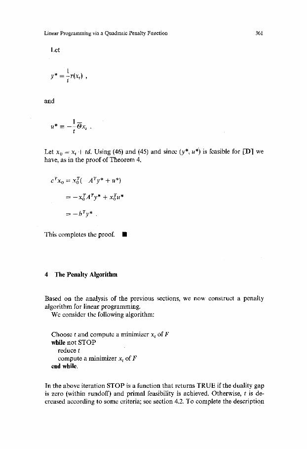
Let

361

y * = ~r(x,) ,

and

1 u , - - - .

t

Let x o = x t + td. Using (46) and (45) and since (y*, u*) is feasible for [D] we have, as in the proof of Theorem 4,

c r x o = x g ( - A r y * + u*)

= - - x T A T y * + x r u *

= - b r y * .

This completes the proof. �9

4 The Penalty Algorithm

Based on the analysis of the previous sections, we now construct a penalty algorithm for linear programming.

We consider the following algorithm:

Choose t and compute a minimizer x t of F while not STOP

reduce t compute a minimizer xt of F

end while.

In the above iteration STOP is a function that returns TRUE if the duality gap is zero (within rundoff) and primal feasibility is achieved. Otherwise, t is de- creased according to some criteria; see section 4.2. To complete the description

362 M. (~. Pinar

we need an algorithm to compute a minimizer of F. Such an algorithm is adapted from the Newton algorithm of [9] for robust linear regression using Huber functions. This algorithm is a standard Newton iteration with a simple line search to solve the nonlinear system of equations F'(x, t) = 0. However, special care must be given to the case where the matrix ATA + -0 is rank- deficient. We give a brief description of the modified Newton algorithm below.

4.1 Computin9 an Unconstrained Minimizer

The algorithm for computing a minimizer xt of F is based on a modified Newton algorithm given in [9]. The idea is to inspect to orthants of ~a" to locate the orthant where the local quadratic Qo contains its own minimizer. This is accom- plished by means of the Newton iteration. At a given iterate, the Newton step is computed using the expansion (12) of F. If a unit step in this direction yields a point in the same orthant, then the global minimizer has been found. I.e., the quadratic representation of F which contains the global minimizer has been located: Otherwise, the algorithm proceeds with a line search.

A search direction h is computed by minimizing the quadratic Q~ where 0 = O(x) and x is the current iterate. More precisely, we consider the equation

Q~h = - Q~(x) (47)

where Q~ and Q~ denote the Hessian and gradient of Qo, respectively. This system is expressed as

(ArA + "O)h = - ( A T A + "O)x + Arb - tc . (48)

For ease of notation let C - ATA + 0 and g - - C x + ATb - tc. Further- more, let ~U(C) denote the null space of C. If C has full rank, then h is the solution to (48). Otherwise, if the system of equations (48) is consistent, a mini- mum norm solution is computed. If the system is inconsistent the projection of g on dV'(C) is computed. These choices are motivated and justified in [9]. The next iterate is found through a line search aiming for a zero of the directional derivative. This procedure is computationally cheap as a result of the piecewise- linear nature of F'. It can be shown using the analysis in [9] that the iteration is finite, i.e., after a finite number of iterations we have x + h ~ C~. Therefore, x + h is a minimizer of F as a result of (11), (12) and the convexity of F. We summarize below the modified Newton algorithm:


repeat

"0 = O(x) if (48) consistent then

find h from (48) if x + h ~ cg~ then

x ~ x + h stop = true

else x ~ x + eh (line search)

endif else

compute h = null space projection of g x ~- x + eh (line search)

endif until stop.

4.2 Reducing t

Let x~ be a minimizer of F(x, t) for some t > 0 and 0 = O(xt). Consider the system

(Ar A + O)d = c . (49)

Let d be a solution to (49). We distinguish between two cases:

Case 1: The duality gap cT(xt + td) + bry * is zero but x t + td is infeasible in [P] , i.e., there existsj such that (xt + td)j < 0. In this case we reduce t as follows. Let q~ --- {"k, k = 1, 2 . . . . . q} be the set of positive kink points where the components o f x t + td change sign, i.e., the set ~t = {0 < a < 113i ~ Jl(xt)i + taidi = O} where J = {i]1 < i _< n ^ dl ~ 0}. I f ~ is non-empty we choose

* = m i n ~k k

and we let

tnext = (1 -- ~*)t ,

and

364

x t , ~ ~ -- x t + c~*td

Otherwise, we let

M. ~;. Pinar

t . ~ t - 0.9t ,

and

x, . . . . =- xt + 0.9td

In both cases, x,.~.~ is used as the starting point of the modified Newton algo- rithrn of section 4.1 with the reduced value of t.

Case 2: The duality gap is not zero. This is an indication that t is not in the interval (0, to]. In this case we reduce t as follows. Let r -= {ak, k = 1, 2 . . . . , q} be the set of positive kink points where the components of x t + td change sign, i.e., the set ~b = {0 < ~ < l l 3 i e J l ( x t ) ~ + te~d i = 0} where J = {ill _< i_< n A d, r 0}. The set r is non-empty as a consequence of Theorem 4. Let at = min~,>o,~,~a / and ~2 = max~,>o,~r and ~* = max{0.1, 0.5(~1 + c~2)}. We u s e

t . ~ , = ( t - ~ * ) t ,

xt . . . . =- xt + ~*td .

For robustness we search only in the interval [OAt, t] so that tnext <_ 0.9t.

5 Finite Convergence

In this section we show that the penalty algorithm of section 4 converges finitely. In the following analysis, an iteration of the algorithm means either a modified Newton iteration or an execution of the t-reduction procedure.

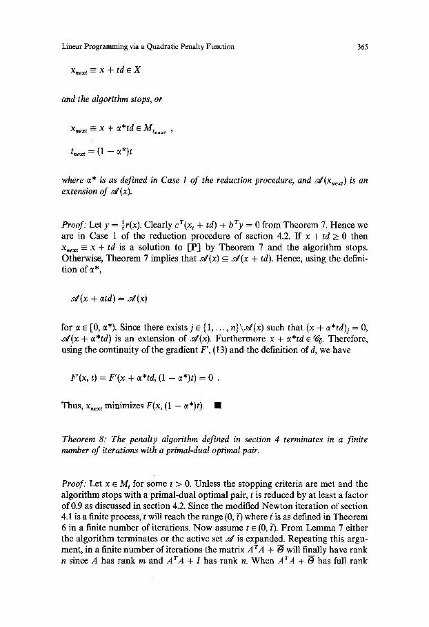
L e m m a 7: A s s u m e t e (0, ?). L e t x ~ Mt wi th 0 = O(x). L e t d solve (49), and x,ex~ be

generated by one iteration o f the penal ty algorithm. Then either


X n e x t ~- X -t- td �9 X

365

and the algorithm stops, or

Xnext = x + e*td �9 Mt.ex t ,

tn~.t = (1 -- a*)t

where ~* is as defined in Case 1 of the reduction procedure, and d(X.ext ) is an extension of x4 (x).

Proof: Let y = ~r(x). Clearly cr(xt + td) + bry = 0 from Theorem 7. Hence we are in Case 1 of the reduction procedure of section 4.2. If x + td > 0 then X,ext- x + td is a solution to [P] by Theorem 7 and the algorithm stops. Otherwise, Theorem 7 implies that ~r c_ d ( x + td). Hence, using the definition of e*,

M(x + etd) = s4(x)

for e e [0, ct*). Since there exists j �9 {1 . . . . . n } \ d ( x ) such that (x + e*td b = O, d ( x + ct*td) is an extension of ~r Furthermore x + e*td e cg~. Therefore, using the continuity of the gradient F', (13) and the definition of d, we have

F'(x, t) = F'(x + e*td, (1 - e*)t) = 0 .

Thus, x,ext minimizes F(x, (1 - e*)t). �9

Theorem 8: The penalty algorithm defined in section 4 terminates in a finite number of iterations with a primal-dual optimal pair.

Proof." Let x ~ Mt for some t > 0. Unless the stopping criteria are met and the algorithm stops with a primal-dual optimal pair, t is reduced by at least a factor of 0.9 as discussed in section 4.2. Since the modified Newton iteration of section 4.1 is a finite process, t will reach the range (0, t--) where ~is as defined in Theorem 6 in a finite number of iterations. Now assume t �9 (0, t-). From Lemma 7 either the algorithm terminates or the active set sr is expanded. Repeating this argument, in a finite number of iterations the matrix ArA + -0 will finally have rank n since A has rank m and ArA + I has rank n. When ArA + -0 has full rank

366 M. ~. Pinar

the solution d to the system (49) is unique, and x,e~t = x + td solves [P] by Theorem 7. �9

6 Numerical Results

In this section we report our numerical experience with a preliminary implementation of the penalty algorithm, which does not exploit sparsity. The implementation was made using the matrix manipulation environment OCTAVE [6] on a SUN 4 Workstation. The purpose of the experiments is to test the viability of the algorithm in solving non-trivial problems. To accomplish this we choose a set of small test problems from the Netlib collection. To get an idea on the relative standing of the penalty algorithm we also compare our results to a linear programming simplex subroutine, E04MBF, from the NAG subroutine library. E04MBF is based on the package LSSOL from Stanford Systems Optimization Library. It is a Fortran 77 package for constrained linear least squares problems, linear programming and convex quadratic programming, [7]. It does not exploit sparsity. Hence, it provides a fair comparison to our numerical results. We perform this comparison only on basis of the number of iterations since (1) we do not yet have an implementation of our algorithm in Fortran 77, and (2) the cost per iteration of the simplex algorithm and the new penalty algorithm are comparable.

Note that the major effort in the Newton algorithm of section 4.1 is spent in solving the systems (48). It is observed that normally only a few entries of the diagonal matrix O change between two consecutive iterations. This implies that the factorization of Ck = A T A --k Ok at iteration k can be obtained by relatively few up- and down-dates of the factorization of Ck_ 1. Using the methods of [13] it can be verified that the computational cost of a typical iteration step is O(n2).

Occasionally, a refactorization may be performed when there is indication of numerical instability or when the estimated computational cost of up- and down-dating the previous factorization outweighs the cost of a refactorization. This is an O(n a) process. Since, a typical iteration of the simplex method involves O(m z) operations, we can conclude that a typical iteration of the penalty method is somewhat more expensive than the simplex method for problems where n > m. In OCTAVE, we have not implemented the up- and down-dating of factorization. This will be done using the ideas of [13] in the future when we have a Fortran 77 implementation of the algorithm.

To initiate the algoritiJm, we choose a starting point x ~ and t o as follows. Let x be a solution to

( A T A q- I ) x = A T b - c .


Then t o is chosen using the following formula:

t o = f l m i n - x i xi #O

where fl ~ (0, 1]. Then, we let x ~ as the solution of

( A r A + I ) x ~ = A r b _ tOc .

Our test problem characteristics are described in Table 1 below (the source for Netlib is [3]). We consider seven problems from the Netlib collection. We also used a test problem from a civil engineering application at the Technical University of Denmark, referred to as plate. All the test problems are put into the form [P] using slack columns.

In Table 2, we show the solution statistics of the penalty method. The columns "iter" and "reduc" refer to the number of iterations and the number of reduc- tions of the parameter t, respectively. The columns t o and t* report the initial and final values of t, respectively. Our stopping criteria are based on the relative duality gap:

Table 1. Characteristics of the test problems

Problem Name Variables Slack Variables Nonzeros in A

afiro

sc50b

sc50a

scl05

adlittle

stocforl

blend

plate

Constraints

27 32

50 48

50 48

105 103

56 97

117 111

74 83

61 73

19

30

30

60

41

54

31

60

83

118

130

280

383

447

491

209

Table 2. Solution statistics of the new penalty algorithm on the test set

Problem Name iter reduc t o t*

afiro

sc50b

sc50a sc105 adlittle

stocforl blend

plate

14

30

31 71

143 62

57

7

1 1 1

11 7

3

2

2.46 x 10 -2

2.45 x 10 ~ 4.47 x 10 -1 2.41 x 10 -3 1.56 x 10 -2

2.40 x 10 -3 2.08 x 10 -2

4.24 x 10 -2

2.46 x 10 -1

2.45 x 10 ~ 4.47 x 10 -1 2.41 x 10 -3 3.88 x 10 -6

8.44 x 10 -4 4.13 x 10 -3

2.05 x 10 -2

368 M.G. Pinar

lcrxl - t b r y ]

1 + Icrx l + Ibry[ '

the values of the components of x, and the smallest component of the residual in the primal constraints:

r = A x - b .

I.e., we stop when the above quantities are less than some tolerances. In all cases reported below, the relative duality gap tolerance is 10 -s, and the feasibility tolerance is 10 -11 In all test cases, the penalty algorithm achieves at least ten correct digits in the optimal objective function value with respect to the known optimal value [3].

We observe that the final value of the penalty parameter varies in the range between 0(10 -6) and O(1). It is also noticed that the half of the problems were solved without the need to reduce t. The problem adlittle required the largest number of t-reduction steps.

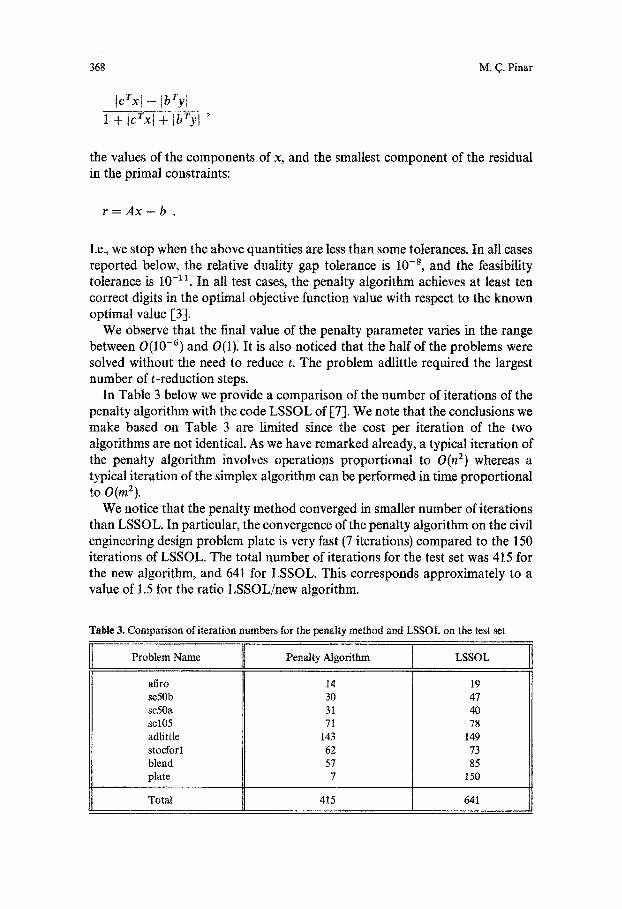
In Table 3 below we provide a comparison of the number of iterations of the penalty algorithm with the code LSSOL of [7]. We note that the conclusions we make based on Table 3 are limited since the cost per iteration of the two algorithms are not identical. As we have remarked already, a typical iteration of the penalty algorithm involves operations proportional to O(n 2) whereas a typical iteration of the simplex algorithm can be performed in time proportional to O(m2).

We notice that the penalty method converged in smaller number of iterations than LSSOL. In particular, the convergence of the penalty algorithm on the civil engineering design problem plate is very fast (7 iterations) compared to the 150 iterations of LSSOL. The total number of iterations for the test set was 415 for the new algorithm, and 641 for LSSOL. This corresponds approximately to a value of 1.5 for the ratio LSSOL/new algorithm.

Table 3. Comparison of iteration numbers for the penalty method and LSSOL on the test set

Problem Name Penalty Algorithm LSSOL

afiro sc50b sc50a scl05 adlittle stocforl blend plate

14 30 31 71

143 62 57 7

19 47 40 78

149 73 85

I50

Total 415 641


7 Conclusions

369

We showed in this paper that the recent ideas from linear 11 estimation [-10] can be successfully used to analyze primal continuous non-interior paths leading to the optimal set of a linear program. Interestingly, these paths yield new characterizations of optimal solutions. We adapted a finite algorithm to perform the unconstrained minimization of F from [-9] where it was developed to solve problems of the form [-SL1]. Using this Newton algorithm we defined a new penalty algorithm for linear programming and proved its finiteness. The computational results indicate that the algorithm is numerically stable and accurate. This suggests that further research is necessary to establish the true potential of the penalty algorithm. Several aspects of the algorithm need further study. Among those, the most important are:

�9 A careful implementation of numerical linear algebra �9 Experimenting with different initialization procedures �9 Experimenting with alternative t-reduction procedures.

Acknowledgements: I would like to thank K. Madsen and H. B. Nielsen for teaching me about their algorithm, and sharing their insights with me. In particular, K. Madsen arranged my two-year visit to the Institute of Mathematical Modelling where this work was done. Special thanks are also due to V. A. Barker for his careful reading of the manuscript.

References

[1] Bartels RH (1980) A penalty linear programming method using reduced-gradient basis- exchange techniques. Linear Algebra Appl 29:17-32

[2] Bertsekas DP (1975) Necessary and sufficient conditions for a penalty method to be exact. Mathematical Programming 9: 87-99

[3] Bixby RE (1990) Implementing the simplex method: Part I: Introduction and Part II: The initial basis. Technical Report TR90-32, Rice University, (also in ORSA J on Computing)

[4] Chebotarev SP (1973) Variation of the penalty coefficient in linear programming problems. Automation and Control 7:102-107

[5] Conn AR (1976) Linear programming via a nondifferentiable penalty function. SIAM J Numer Anal 13:145-154

[6] Eaton JW (1993) OCTAVE: A high-level interactive language for numerical computations. Manuscript University of Texas at Austin

[7] Gill PE, Hammarling S, Murray W, Saunders MA, Wright MH (1986) User's guide for LSSOL (Version 1.0): A fortran package for constrained linear least squares and convex quadratic programming. Report SOL 86-1, Department of Operations Research, Stanford University, Stanford, CA

[8] Huber P (1981) Roubust statistics. John Wiley, New York

370 M. ~. Pinar

I-9] Madsen K, Nielsen HB (1990) Finite algorithms for robust linear regression. BIT 30:682-699 1-10] Madsen K, Nielsen HB, Pinar MC (1993) New characterizations of 11 solutions of overdeter-

mined linear systems. Operations Research Letters 16:159-166 [11] Mangasarian OL (1986) Some applications of penalty functions in mathematical program-

ming. Lecture Notes in Mathematics, No 1190. In: Conti R, De Giorgi E, Giannessi F (eds), Optimization and Related Fields. Springer-Verlag, Berlin 307-329

[12] Murty KG (1976) Linear and combinatorial programming. John Wiley & Sons, New York [13] Nielsen HB (1990) AAFAC: A package of fortran 77 subprograms for solving A r A x = c.

Report NI-90-11. Institute for Numerical Analysis, Technical University of Denmark [14] Pietrzykowski T (1961) Application of the steepest ascent method to linear programming.

PRACE ZAM A 11 [15] Pinar M~ Piecewise-linear pathways to the optimal set in linear programming. Technical

Report, Bilkent University, 1996

Received: February 1995 Revised version received: May 1995

Linear programming via a quadratic penalty...

Documents

Transcript of Linear programming via a quadratic penalty...