LINEAR PROGRAMMING SOLUTION TECHNIQUES: GRAPHICAL AND COMPUTER METHODS.

LINEAR PROGRAMMING LINEAR PROGRAMMING SOLUTION TECHNIQUES: SOLUTION TECHNIQUES:

GRAPHICAL AND COMPUTER GRAPHICAL AND COMPUTER METHODS METHODS

LEARNING OBJECTIVESLEARNING OBJECTIVES

Understand basic assumptions and properties of linear

programming (LP).

Use graphical solution procedures for LP problems with

only two variables to understand how LP problems are

solved.

Understand special situations such as redundancy,

infeasibility, unboundedness, and alternate optimal

solutions in LP problems.

Understand how to set up LP problems on a spreadsheet

and solve them using Excel’s solver.

INTRODUCTIONINTRODUCTION Management decisions in many organizations involve trying

to make most effective use of resources (machinery, labor,

money, time, warehouse space, and raw materials) in order

to:

Produce products - such as computers, automobiles, or

clothing or

Provide services - such as package delivery, health

services, or investment decisions.

To solve problems of resource allocation one may use

mathematical programming.

LINEARLINEAR PROGRAMMING PROGRAMMING

Linear programming (LP) is the most common type of

mathematical programming.

LP seeks to maximize or minimize a linear objective

function subject to a set of linear constraints

LP assumes all relevant input data and parameters are

known with certainty (deterministic models).

Computers play an important role in the solution of LP

problems

Decision variables - mathematical symbols representing levels of activity of a firm.

Objective function - a linear mathematical relationship describing an objective of the firm, in terms of decision variables, that is to be maximized or minimized

Constraints - restrictions placed on the firm by the operating environment stated in linear relationships of the decision variables.

Parameters - numerical coefficients and constants used in the objective function and constraint equations.

LP MODEL COMPONENTS AND LP MODEL COMPONENTS AND FORMULATIONFORMULATION

DDEVELOPMENT OF A LP MODELEVELOPMENT OF A LP MODEL

LP applied extensively to problems areas - medical, transportation, operations, financial, marketing, accounting, human resources, and agriculture.

Development and solution of all LP models can be examined in a four step process:

(1) identification of the problem as solvable by LP

(2) formulation of the mathematical model.

(3) solution.

(4) interpretation.

BASIC STEPS OF DEVELOPING A LP BASIC STEPS OF DEVELOPING A LP MODELMODEL

Formulation– Process of translating problem scenario into simple LP model

framework with a set of mathematical relationships.

Solution – Mathematical relationships resulting from formulation process are

solved to identify optimal solution.

Interpretation and What-if Analysis – Problem solver or analyst works with the manager to

interpret results and implications of problem solution.

investigate changes in input parameters and model variables and impact on problem solution results.

LLINEAR EQUATIONS AND INEAR EQUATIONS AND INEQUALITIESINEQUALITIES

This is a linear equation:

2A + 5B = 10

This equation is not linear:

2A2 + 5B3 + 3AB = 10

LP uses, in many cases, inequalities like:

A + B C or A + B C

BBASIC ASSUMPTIONS OF A LP MODELASIC ASSUMPTIONS OF A LP MODEL

1. Conditions of certainty exist.

2. Proportionality in objective function and constraints (1 unit – 3 hours, 3 units- 9 hours).

3. Additivity (total of all activities equals sum of individual activities).

4. Divisibility assumption that solutions need not necessarily be in whole numbers (integers); ie.decision variables can take on any fractional value.

FORMULATING A LP PROBLEMFORMULATING A LP PROBLEM A common LP application is product mix problem.

– Two or more products are usually produced using

limited resources - such as personnel, machines, raw

materials, and so on.

Profit firm seeks to maximize is based on profit

contribution per unit of each product.

Firm would like to determine -

– How many units of each product it should produce in

order to maximize overall profit given its limited

resources.

MAXIMIZATION MODEL EXAMPLES:MAXIMIZATION MODEL EXAMPLES:

BEAVER CREEK EXAMPLEBEAVER CREEK EXAMPLE FLAIR FURNITURE EXAMPLEFLAIR FURNITURE EXAMPLE GALAXY INDUSTRIES EXAMPLEGALAXY INDUSTRIES EXAMPLE

Resource Requirements

Product Labor

(hr/unit) Clay

(lb/unit) Profit

($/unit)

Bowl 1 4 40

Mug 2 3 50

PPROBLEM DEFINITION:ROBLEM DEFINITION:BEAVER CREEK MAXIMIZATION BEAVER CREEK MAXIMIZATION PROBLEM PROBLEM (1 of (1 of 18)18)

Product mix problem - Beaver Creek Pottery Company

How many bowls and mugs should be produced to maximize profits given labor and materials constraints?

Product resource requirements and unit profit:

PPROBLEM DEFINITION: ROBLEM DEFINITION: BBEAVER EAVER CREEK EXAMPLECREEK EXAMPLE (2 of (2 of 1818))

Resource 40 hrs of labor per dayAvailability: 120 lbs of clay

Decision Variables x1 = number of bowls to produce per day x2 = number of mugs to produce per day

Objective Maximize Z = $40x1 + $50x2

Function: Where Z = profit per day

Resource 1x1 + 2x2 40 hours of laborConstraints: 4x1 + 3x2 120 pounds of clay

Non-Negativity x1 0; x2 0 Constraints:

PPROBROBLLEM DEFINITIONEM DEFINITION::BBEAVER CREEK EXAMPLEEAVER CREEK EXAMPLE (3 of (3 of 1818))

Complete Linear Programming Model:

Maximize Z = $40x1 + $50x2

subject to: 1x1 + 2x2 40

4x1 + 3x2 120

x1, x2 0

A feasible solution does not violate any of the constraints:

Example x1 = 5 bowls

x2 = 10 mugs

Z = $40x1 + $50x2 = $700

Labor constraint check:

1(5) + 2(10) = 25 < 40 hours, within constraint

Clay constraint check:

4(5) + 3(10) = 50 < 120 pounds, within constraint

FEASIBLE SOLUTIONS:FEASIBLE SOLUTIONS:BBEAVER CREEK EXAMPLE (4EAVER CREEK EXAMPLE (4 of of 1818))

An infeasible solution violates at least one of the constraints:

Example x1 = 10 bowls

x2 = 20 mugs

Z = $1400

Labor constraint check:

1(10) + 2(20) = 50 > 40 hours, violates the constraint

IINFEASIBLE SOLUTIONS:NFEASIBLE SOLUTIONS:BBEAVER CREEK EXAMPLEEAVER CREEK EXAMPLE ( (55 of of 1818))

The set of all points that satisfy all the constraints of the model is called

a

FEASIBLE REGIONFEASIBLE REGION

Graphical solution is limited to linear programming models containing only two decision variables (can be used with three variables but only with great difficulty).

Graphical methods provide visualization of how a solution for a linear programming problem is obtained.

GGRAPHICAL SOLUTION OF LRAPHICAL SOLUTION OF LIINEAR NEAR PROGRAMMING MODELSPROGRAMMING MODELS

Primary advantage of two-variable LP models (such as

Beaver Creek problem) is their solution can be graphically

illustrated using two-dimensional graph.

Allows one to provide an intuitive explanation of how

more complex solution procedures work for larger LP

models.

GRAPHICAL REPRESENTATION OF LP GRAPHICAL REPRESENTATION OF LP MODELSMODELS

Coordinates for graphical analysis 10

20

30

40

50

60

10 20 30 40 50 600

GGRAPHRAPHIICAL REPRESENTATION OF CAL REPRESENTATION OF CONSTRAINTS:CONSTRAINTS:COORDINATE ACOORDINATE AXEXESS-B-BEAVER CREEK EAVER CREEK EXAMPLE (6 EXAMPLE (6 oof f 118)8)


subject to: 1x1 + 2x2 40 4x1 + 3x2 120

x1, x2 0

Coordinates for Graphical Analysis

GGRAPHRAPHIICAL REPRESENTATION OF CAL REPRESENTATION OF CONSTRAINTS:CONSTRAINTS:-B-BEAVER CREEK EXAMPLE-LABOR EAVER CREEK EXAMPLE-LABOR CONSTRAINT (CONSTRAINT (77 oof f 118)8)


subject to: 1x1 + 2x2 40 4x1 + 3x2 120

x1, x2 0

Graph of Labor Constraint

GGRAPHRAPHIICAL REPRESENTATION OF CAL REPRESENTATION OF CONSTRAINTS:CONSTRAINTS:-B-BEAVER CREEK EXAMPLE-LABOR EAVER CREEK EXAMPLE-LABOR CONSTRAINT AREA(CONSTRAINT AREA(88 oof f 118)8)


subject to: 1x1 + 2x2 40 4x1 + 3x2 120

x1, x2 0

Labor Constraint Area

GGRAPHRAPHIICAL REPRESENTATION OF CAL REPRESENTATION OF CONSTRAINTS:CONSTRAINTS:BBEAVER CREEK EXAMPLE-CLAY EAVER CREEK EXAMPLE-CLAY CONSTRAINT AREA(9 CONSTRAINT AREA(9 oof f 118)8)


subject to: 1x1 + 2x2 40 4x1 + 3x2 120

x1, x2 0

Clay Constraint Area


subject to: 1x1 + 2x2 40 4x1 + 3x2 120

x1, x2 0

Graph of Both Model Constraints

GGRAPHRAPHIICAL REPRESENTATION OF CAL REPRESENTATION OF CONSTRAINTS:CONSTRAINTS:BBEAVER CREEK EXAMPLE- BOTH EAVER CREEK EXAMPLE- BOTH CONSTRAINTS (CONSTRAINTS (110 0 oof f 118)8)

FFEASIBLE SOLUTION AREA:EASIBLE SOLUTION AREA:BBEAVER CREEK EEAVER CREEK EXXAMPLE AMPLE ((1111 of 1of 188))


subject to: 1x1 + 2x2 40 4x1 + 3x2 120

x1, x2 0

Feasible Solution Area

GGRAPHICAL SOLUTION: RAPHICAL SOLUTION: ISOPROFIT LINE SOLUTION METHODISOPROFIT LINE SOLUTION METHOD

Optimal solution is the point in feasible region that produces highest profit

There are many possible solution points in region.

How do we go about selecting the best one, one yielding

highest profit?

Let objective function (that is, $$40x1 + $50x2) guide one

towards optimal point in feasible region.

Plot line representing objective function on graph as a

straight line.

IISOPROFSOPROFIIT LT LIINE METHOD:NE METHOD:BBEAVER CREEK EXAMPLEEAVER CREEK EXAMPLE ( (112 of 12 of 188))


subject to: 1x1 + 2x2 40 4x1 + 3x2 120

x1, x2 0

Objective Function Line for Z = $800

Set Objective Function = 800

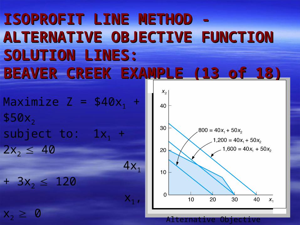
ISOPROFIT LINE METHODISOPROFIT LINE METHOD - - ALTERNATIVE OBJECTIVE FUNCTION ALTERNATIVE OBJECTIVE FUNCTION SOLUTION LSOLUTION LIINES:NES:BEAVER CREEK EXAMPLEBEAVER CREEK EXAMPLE ( (1133 of 1of 188))


subject to: 1x1 + 2x2 40 4x1 + 3x2 120

x1, x2 0

Alternative Objective Function Lines

ISOPROFIT LINEISOPROFIT LINE MEMETTHOD-HOD-OOPTIMAL PTIMAL SOLUTION):SOLUTION):BBEAVER CREEK EXAMPLE EAVER CREEK EXAMPLE ((114 of 14 of 188))


subject to: 1x1 + 2x2 40 4x1 + 3x2 120

x1, x2 0

Identification of the Optimal Solution

ISOPROFIT LINE METHODISOPROFIT LINE METHOD - OPT- OPTIIMAL MAL SOLUTION COORDINATES:SOLUTION COORDINATES:BEBEAAVER CREEK EXAMPLEVER CREEK EXAMPLE (15 (15 of 1of 188))


subject to: 1x1 + 2x2 40 4x1 + 3x2 120

x1, x2 0

Optimal Solution Coordinates

CCORNER POINT PROPERTYORNER POINT PROPERTY

It is a very important property of Linear Programming problems:

This property states optimal solution to LP problem will always occur at a corner point.

GGRAPHICAL SOLUTIRAPHICAL SOLUTIOON N -- CORNER CORNER POPOIINT SOLUTION METHODNT SOLUTION METHOD ::BBEAEAVER CREVER CREEEK EXAMPLEK EXAMPLE(1(166 of 1 of 188))


subject to: 1x1 + 2x2 40 4x1 + 3x2 120

x1, x2 0

Solution at All Corner Points

OOPTPTIIMAL SOLUTION FOR A NEW MAL SOLUTION FOR A NEW OBJECTIVE FUNCTION: OBJECTIVE FUNCTION: BBEAVER CREEK EXAMPLEEAVER CREEK EXAMPLE (1 (177 of 1 of 188))


subject to: 1x1 + 2x2 40 4x1 + 3x2 120

x1, x2 0

Optimal Solution with Z = 70x1 + 20x2

Standard form requires that all constraints be in the form of equations.

A slack variable is added to a constraint to convert it to an equation (=).

A slack variable represents unused resources.

A slack variable contributes nothing to the objective function value.

SLACK VARIABLESSLACK VARIABLES

SSTANDARD FORM OF LTANDARD FORM OF LIINEAR NEAR PROGRPROGRAAMMIMMINNG MODEL:G MODEL:BEAVER CREEK EXAMPLE (18 of 18)BEAVER CREEK EXAMPLE (18 of 18)

Max Z = 40x1 + 50x2 + s1 +s2

subject to:1x1 + 2x2 + s1 = 40 4x1 + 3x2 + s2 = 120 x1, x2, s1, s2 0Where:

x1 = number of bowls x2 = number of mugs s1, s2 are slack variables

Solution Points A, B, and C with Slack

PROBLEM DEFINITION:PROBLEM DEFINITION:FLAIR FURNITURE MAXIMIZATION FLAIR FURNITURE MAXIMIZATION EXAMPLEEXAMPLE (1 of 19) (1 of 19) Company Data and Constraints -

Flair Furniture Company produces tables and chairs.

Each table requires: 4 hours of carpentry and 2 hours of painting.

Each chair requires: 3 hours of carpentry and 1 hour of painting.

Available production capacity: 240 hours of carpentry time and 100 hours of painting time.

Due to existing inventory of chairs, Flair is to make no more than 60 new chairs.

Each table sold results in $7 profit, while each chair produced yields $5 profit.

Flair Furniture’s problem:

Determine the best possible combination of tables and chairs to manufacture in order to attain maximum profit.

DECISION VARIABLES: DECISION VARIABLES: FLAIR FURNITURE EXAMPLEFLAIR FURNITURE EXAMPLE (2 of 19) (2 of 19)

Problem facing Flair is to determine how many chairs

and tables to produce to yield maximum profit?

In Flair Furniture problem, there are two unknown

entities:

T- number of tables to be produced.

C- number of chairs to be produced.

OBJECTIVE FUNCTION:OBJECTIVE FUNCTION:FLAIR FURNITURE EXAMPLE FLAIR FURNITURE EXAMPLE (3 of 19)(3 of 19)

Objective function states the goal of problem.

What major objective is to be solved?

Maximize profit!

An LP model must have a single objective function.

In Flair’s problem, total profit may be expressed as:

Using decision variables T and C -

Maximize $7 T + $5 C

($7 profit per table) x (number of tables produced) + ($5 profit per chair) x (number of chairs produced)

CONSTRAINTS:CONSTRAINTS: FLAIR FURNITURE EXAMPLE FLAIR FURNITURE EXAMPLE (4 of 19)(4 of 19)

Denote conditions that prevent one from selecting any

specific subjective value for decision variables.

In Flair Furniture’s problem, there are three

restrictions on solution.

Restrictions 1 and 2 have to do with available

carpentry and painting times, respectively.

Restriction 3 is concerned with upper limit on the

number of chairs.

CONSTRAINTS:CONSTRAINTS: FLAIR FURNITURE EXAMPLE FLAIR FURNITURE EXAMPLE (5 of 19)(5 of 19)

There are 240 carpentry hours available. 4T + 3C < 240

There are 100 painting hours available. 2T + 1C 100

The marketing specified chairs limit constraint. C 60

The non-negativity constraints. T 0 (number of tables produced is 0) C 0 (number of chairs produced is 0)

BUILDING THE COMPLETE BUILDING THE COMPLETE MATHEMATICAL MODEL:MATHEMATICAL MODEL: FLAIR FURNITURE EXAMPLE (6 oFLAIR FURNITURE EXAMPLE (6 of 19)f 19)

Maximize profit = $7T + $5C (objective function)

Subject to constraints -

4T + 3C 240 (carpentry constraint)

2T + 1C 100 (painting constraint)

C 60 (chairs limit constraint)

T 0 (non-negativity constraint on tables)

C 0 (non-negativity constraint on chairs)

CONVERTING INEQUALITIES INTO CONVERTING INEQUALITIES INTO EQUALITIES BY USING SLACK:EQUALITIES BY USING SLACK:FLAIR FURNITURE EXAMPLE (7 of 19)FLAIR FURNITURE EXAMPLE (7 of 19)

Maximize profit = $7T + $5C + 0s1 + 0s2 + 0s3

Subject to constraints -

4T + 3C + s1 = 240 (carpentry constraint)

2T + 1C + s2 = 100 (painting constraint)

C + s3 = 60 (chairs limit constraint)

T 0 (non-negativity constraint on tables)

C 0 (non-negativity constraint on chairs) s1 s2 s3 0 (non-negativity constraints on slacks)

GRAPHICAL REPRESENTATION OF GRAPHICAL REPRESENTATION OF CONSTRAINTS:CONSTRAINTS:FLAIR FURNITURE EXAMPLE (8 of 19)FLAIR FURNITURE EXAMPLE (8 of 19)

4T + 3C 240

Carpentry time constaint


Carpentry Time ConstraintCarpentry Time Constraint (feasible area)(feasible area)Carpentry time and

the feasible region

Any point below line satisfies constraint.


Painting Time Constraint and the Feasible Area

2T + 1C 100

Any point on line satisfies equation:2T + 1C = 100(30,40) yields 100.

Any point below line satisfies constraint.


Chair Limit Constraint and the Feasible Solution Area

Feasible solution area is constrained by three limiting lines

IISOPROFIT LINE SOLUTION METHOD:SOPROFIT LINE SOLUTION METHOD: FLAIR FURNITURE EXAMPLE (12 of 19) FLAIR FURNITURE EXAMPLE (12 of 19)

Let objective function (that is, $7T + $5C) guide one

towards an optimal point in the feasible region.

Plot line representing objective function on graph.

One does not know what $7T + $5C equals at an optimal

solution.

Without knowing this value, how does one plot

relationship?


Write objective function: $7 T + $5 C = Z

Select any arbitrary value for Z.

For example, one may choose a profit ( Z ) of $210.

Z is written as: $7 T + $5 C = $210.

To plot this profit line:

Set T = 0 and solve objective function for C.

Let T = 0, then $7(0) + $5C = $210, or C = 42.

Set C = 0 and solve objective function for T.

Let C = 0, then $7T + $5(0) = $210, or T = 30.


One can check for higher values of Z to find an optimal solution.

210 is not the highest possible value.


Isoprofit lines ($210, $280, $350) are all parallel.


Optimal Solution:Corner Point 4: T=30 (tables) and C=40 (chairs) with $410 profit


Optimal solution occurs at the maximum point in the feasible region.

It occurs at the intersection of carpentry and painting constraints:

- Carpentry constraint equation: 4T + 3C = 240

- Painting constraint equation : 2T + 1C = 100

If one solves these two equations with two unknowns for T

and C (for Corner Point 4), Optimal Solution is found:

T=30 (tables) and C=40 (chairs) with $410 profit.

CORNER POINT SOLUTION METHOD:CORNER POINT SOLUTION METHOD:FLAIR FURNITURE EXAMPLEFLAIR FURNITURE EXAMPLE (18 of 19) (18 of 19)

From the figure one knows that the feasible region for Flair’s problem has five corner points, namely, 1, 2, 3, 4, and 5, respectively.

To find the point yielding the maximum profit, one finds coordinates of each corner point and computes profit level at each point.

CORNER POINT SOLUTION METHOD:CORNER POINT SOLUTION METHOD:FLAIR FURNITURE EXAMPLEFLAIR FURNITURE EXAMPLE (19 of 19) (19 of 19)

Point 1 (T = 0, C = 0) profit = $7(0) + $5(0) = $0

Point 2 (T = 0, C = 60) profit = $7(0) + $5(60) = $300

Point 3 (T = 15, C = 60) profit = $7(15) + $5(60) = $405

Point 4 (T = 30, C = 40) profit = $7(30) + $5(40) = $410

Point 5 (T = 50, C = 0) profit = $7(50) + $5(0) = $350 .

PROBLEM DEFINITION:PROBLEM DEFINITION:THE GALAXY INDUSTRIES EXAMPLE THE GALAXY INDUSTRIES EXAMPLE (1 of 9)(1 of 9)

Galaxy manufactures two toy models:– Space Ray. – Zapper.

Resources are limited to

– 1200 pounds of special plastic.– 40 hours of production time per week.

Marketing requirement– Total production cannot exceed 800 dozens.

– Number of dozens of Space Rays cannot exceed

number of dozens of Zappers by more than 450.

Technological input– Space Rays requires 2 pounds of plastic and

3 minutes of labor per dozen.– Zappers requires 1 pound of plastic and

4 minutes of labor per dozen.


Current production plan calls for: – Producing as much as possible of the more profitable

product, Space Ray ($8 profit per dozen).– Use resources left over to produce Zappers ($5 profit

per dozen).

The current production plan consists of:

Space Rays = 550 dozens Zapper = 100 dozens Profit = 4900 dollars per week


Management is seeking a production schedule that will increase the company’s

profit.

Decision variables:– X1 = Production level of Space Rays (in dozens per

week).– X2 = Production level of Zappers (in dozens per week).

Objective Function:

- Weekly profit, to be maximized

DECISION VARIABLES:DECISION VARIABLES:GALAXY INDUSTRIES EXAMPLE GALAXY INDUSTRIES EXAMPLE (4 of 9) (4 of 9)

Max. 8X1 + 5X2 (Weekly profit)

subject to

2X1 + 1X2 < = 1200 (Plastic)

3X1 + 4X2 < = 2400 (Production Time)

X1 + X2 < = 800 (Total production)

X1 - X2 < = 450 (Mix)

Xj> = 0, j = 1,2 (Nonnegativity)

BUILDING THE COMPLETE BUILDING THE COMPLETE MATHEMATICAL MODEL: MATHEMATICAL MODEL: GALAXY INDUSTRIES EXAMPLE GALAXY INDUSTRIES EXAMPLE (5 of 9)(5 of 9)

1200

600

The Plastic constraint

Feasible

The plastic constraint: 2X1+X2<=1200

X2

Infeasible

Production Time3X1+4X2<=2400

Total production constraint: X1+X2<=800

600

800

Production mix constraint:X1-X2<=450

• There are three types of feasible pointsInterior points.

Boundary points.

Extreme points.

X1

GRAPHICAL REPRESENTATION OF GRAPHICAL REPRESENTATION OF CONSTRAINTS:CONSTRAINTS:GALAXY INDISTRIES EXAMPLE (6 of 9)GALAXY INDISTRIES EXAMPLE (6 of 9)

SOLVING GRAPHICALLY FOR AN SOLVING GRAPHICALLY FOR AN OPTIMAL SOLUTIONOPTIMAL SOLUTION

Recall the feasib

le Region

600

800

1200

400 600 800

X2

X1

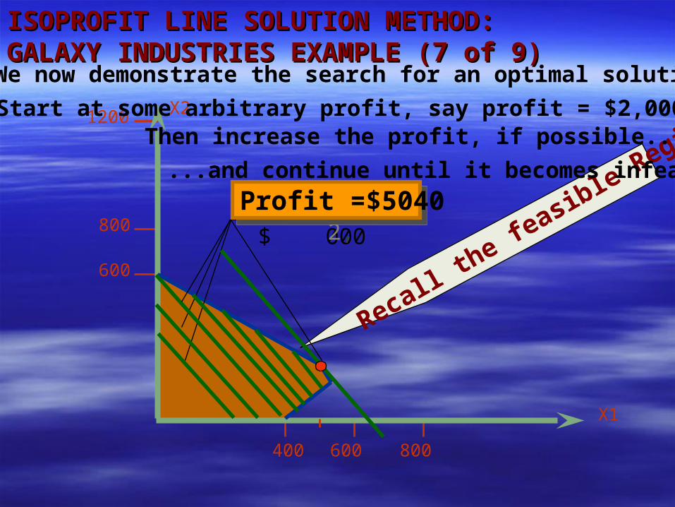
We now demonstrate the search for an optimal solution

Start at some arbitrary profit, say profit = $2,000...

Profit = $ 000

2,

Then increase the profit, if possible...

3,4,

...and continue until it becomes infeasible

Profit =$5040

ISOPROFIT LINE SOLUTION METHOD:ISOPROFIT LINE SOLUTION METHOD:GALAXY INDUSTRIES EXAMPLE (7 of 9)GALAXY INDUSTRIES EXAMPLE (7 of 9)

600

800

1200

400 600 800

X2

X1

Let’s take a closer look at the optimal point

FeasibleregionFeasibleregion

Infeasible

ISOPROFIT LINE SOLUTION METHOD:ISOPROFIT LINE SOLUTION METHOD:GALAXY INDUSTRIES EXAMPLE (8 of 9)GALAXY INDUSTRIES EXAMPLE (8 of 9)

OPTIMAL SOLUTION:OPTIMAL SOLUTION:GALAXY INDUSTRIES EXAMPLE (9 of 9)GALAXY INDUSTRIES EXAMPLE (9 of 9)

Space Rays = 480 dozens Zappers = 240 dozens Profit = $5040

– This solution utilizes all the plastic and all the production

hours.

– Total production is only 720 (not 800).

– Space Rays production exceeds Zapper by only 240

dozens (not 450).

MINIMIZATION MODEL EXAMPLES:MINIMIZATION MODEL EXAMPLES: FERTILIZER MIX PROBLEMFERTILIZER MIX PROBLEM HOLIDAY MEAL CHICKEN RANCH HOLIDAY MEAL CHICKEN RANCH

EXAMPLEEXAMPLE NAVY SEA RATIONS EXAMPLENAVY SEA RATIONS EXAMPLE

A A MINIMIZATION LP PROBLEMMINIMIZATION LP PROBLEM

Many LP problems involve minimizing objective such as cost

instead of maximizing profit function.

Examples:

– Restaurant may wish to develop work schedule to meet staffing

needs while minimizing total number of employees.

– Manufacturer may seek to distribute its products from several

factories to its many regional warehouses in such a way as to

minimize total shipping costs.

– Hospital may want to provide its patients with a daily meal plan

that meets certain nutritional standards while minimizing food

purchase costs.

PPROBLEM ROBLEM DDEFINITION:EFINITION:FERTILIZER MFERTILIZER MIIX EXAMPLE X EXAMPLE (1 of 7)(1 of 7)

Chemical Contribution

Brand Nitrogen (lb/bag)

Phosphate (lb/bag)

Super-gro 2 4

Crop-quick 4 3

Two brands of fertilizer available - Super-Gro, Crop-Quick.

Field requires at least 16 pounds of nitrogen and 24 pounds of phosphate.

Super-Gro costs $6 per bag, Crop-Quick $3 per bag.

Problem: How much of each brand to purchase to minimize total cost of fertilizer given the following data ?

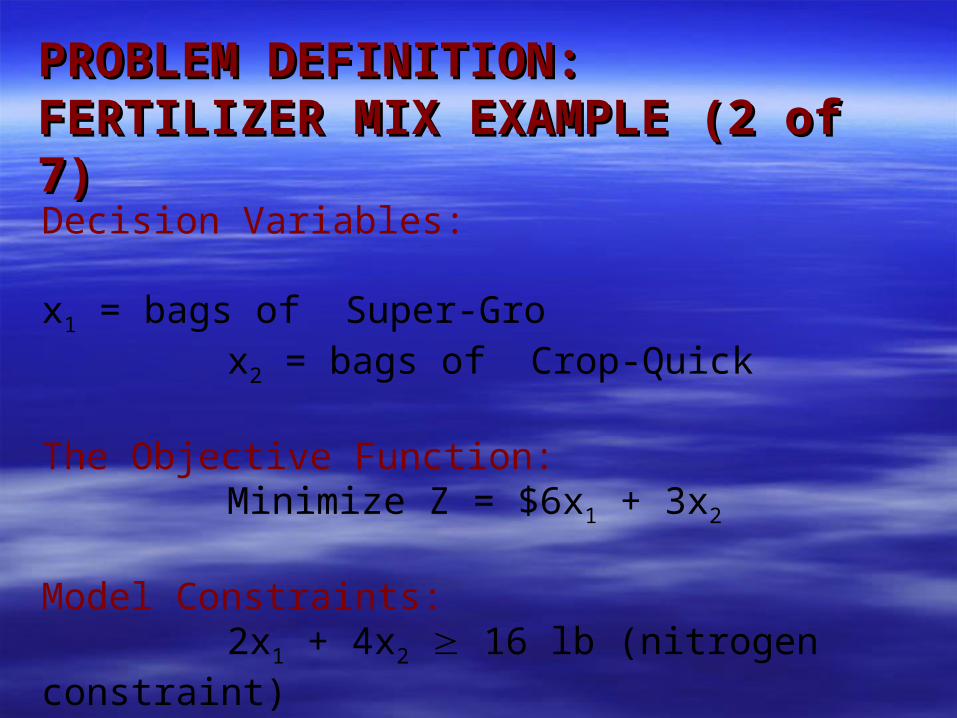
PPROBLEM ROBLEM DDEFINITION:EFINITION:FERTILIZER MFERTILIZER MIIX EXAMPLE X EXAMPLE ((22 of 7) of 7)

Decision Variables: x1 = bags of Super-Gro

x2 = bags of Crop-Quick

The Objective Function:Minimize Z = $6x1 + 3x2

Model Constraints:2x1 + 4x2 16 lb (nitrogen constraint)4x1 + 3x2 24 lb (phosphate constraint)x1, x2 0 (non-negativity constraint)

GRAGRAPPHICAL REPRESENTATION OF HICAL REPRESENTATION OF CONSTRAINTS:CONSTRAINTS:FERTILIZER MIX EXAMPLEFERTILIZER MIX EXAMPLE (3 of 7) (3 of 7)

Minimize Z = $6x1 + $3x2

subject to: 2x1 + 4x2 16 4x2 + 3x2 24

x1, x2 0

Graph of Both Model Constraints

FFEASIBLE SOLUTION AREA:EASIBLE SOLUTION AREA:FERTILIZER FERTILIZER MIMIX EXAMPLEX EXAMPLE (4 of 7) (4 of 7)


subject to: 2x1 + 4x2 16 4x2 + 3x2 24

x1, x2 0

Feasible Solution Area

OOPTIMAL SOLUTION POPTIMAL SOLUTION POIINT:NT:FERTILIZFERTILIZEER MIX EXR MIX EXAAMPLEMPLE (5 of 7) (5 of 7)


subject to: 2x1 + 4x2 16 4x2 + 3x2 24

x1, x2 0

Optimum Solution Point

SSURPLUS VARIURPLUS VARIAABLES:BLES:FFERTILIZER MIX EXAMPLEERTILIZER MIX EXAMPLE (6 of 7) (6 of 7) A surplus variable is subtracted from a constraint to

convert it to an equation (=).

A surplus variable represents an excess above a constraint requirement level.

Surplus variables contribute nothing to the calculated value of the objective function.

Subtracting surplus variables in the farmer problem constraints:

2x1 + 4x2 - s1 = 16 (nitrogen)

4x1 + 3x2 - s2 = 24 (phosphate)

Minimize Z = $6x1 + $3x2 + 0s1 + 0s2

subject to: 2x1 + 4x2 – s1 = 16 4x2 + 3x2 – s2 = 24

x1, x2, s1, s2 0

Graph of Fertilizer Example

GRAPHICAL SOLUTION:GRAPHICAL SOLUTION:FFERTILIZER MIX EXAMPLEERTILIZER MIX EXAMPLE (7 of 7) (7 of 7)

PROBLEM DEFINITION:PROBLEM DEFINITION:HOLIDAY MEAL CHICKEN RANCH HOLIDAY MEAL CHICKEN RANCH (HMCR) EXAMPLE (1 of 10)(HMCR) EXAMPLE (1 of 10)

Buy two brands of feed for good, low-cost diet for chickens. Each feed may contain three nutritional ingredients (protein, vitamin,

and iron). One pound of Brand A contains:

5 units of protein, 4 units of vitamin, and 0.5 units of iron.

One pound of Brand B contains: 10 units of protein, 3 units of vitamin, and 0 units of iron.

PROBLEM DEFINITION:PROBLEM DEFINITION:HMCR EXAMPLE (2 of 10)HMCR EXAMPLE (2 of 10)

Brand A feed costs ranch $0.02 per pound, while Brand B

feed costs $0.03 per pound.

Ranch owner would like lowest-cost diet that meets

minimum monthly intake requirements for each

nutritional ingredient.

PROBLEM DEFINITION:PROBLEM DEFINITION:HMCR EXAMPLE (3 of 10)HMCR EXAMPLE (3 of 10)

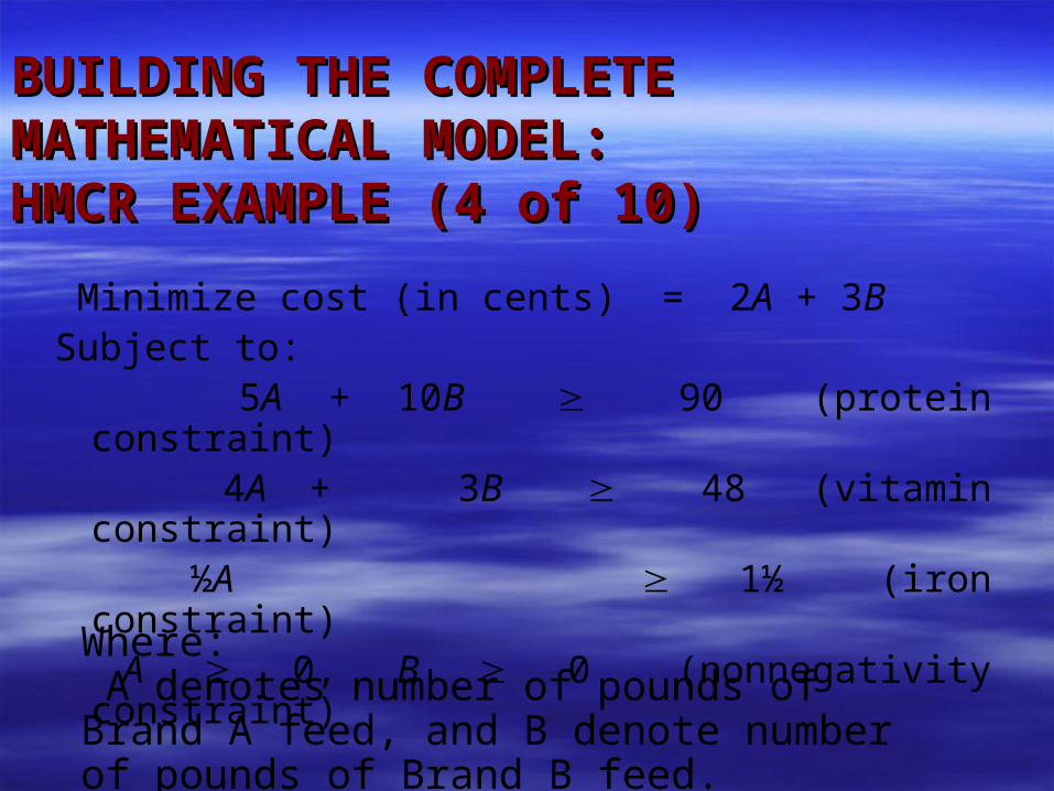
BUILDING THE COMPLETE BUILDING THE COMPLETE MATHEMATICAL MODEL:MATHEMATICAL MODEL:HMCR EXAMPLE (4 of 10)HMCR EXAMPLE (4 of 10)

Minimize cost (in cents) = 2A + 3BSubject to: 5A + 10B 90 (protein constraint) 4A + 3B 48 (vitamin constraint) ½A 1½ (iron constraint) A 0, B 0 (nonnegativity constraint)

Where: A denotes number of pounds of Brand A feed, and B denote number of pounds of Brand B feed.

BUILDING THE STANDARD LP MODEL:BUILDING THE STANDARD LP MODEL:HMCR EXAMPLE (5 of 10)HMCR EXAMPLE (5 of 10)

Minimize cost (in cents)=2A+3B+0s1+0s2+0s3

subject to constraints:

5A + 10B - s1 = 90 (protein constraint)

4A + 3B - s2 = 48 (vitamin constraint)

½A - s3 = 1½ (iron constraint)

A, B, s1,s2 s3 0 (nonnegativity)

GRAPHICAL REPRESENTATION OF GRAPHICAL REPRESENTATION OF CONSTRAINTS:CONSTRAINTS:HMCR EXAMPLE (6 of 10)HMCR EXAMPLE (6 of 10)

Drawing Constraints:

5A + 10B 90

4A + 3B 48

½A 1½

Nonnegativity Constraint A 0, B 0

GRAPHICAL SOLUTION METHOD-ISOCOST GRAPHICAL SOLUTION METHOD-ISOCOST LINE METHOD: HMCR EXAMPLE (7 of 10)LINE METHOD: HMCR EXAMPLE (7 of 10)

One can start by drawing a 54-cent cost line : 2A + 3B. = 54

ISOCOST LINE METHOD:ISOCOST LINE METHOD:HMCR EXAMPLE (8 of 10)HMCR EXAMPLE (8 of 10)

Isocost line is moved parallel to 54-cent solution line toward lower left origin. Last point to touch the isocost line while still in contact with the feasible

region, is corner point 2.

• Solving for corner point 2 with two equations produces values 8.4 for A and 4.8 for B, minimum optimal cost solution is:

2A + 3B = (2)(8.4) + (3)(4.8) = 31.2

IISOCOST LINE METHOD:SOCOST LINE METHOD:HMCR EXAMPLE (9 of 10)HMCR EXAMPLE (9 of 10)

CORNER POINT SOLUTION CORNER POINT SOLUTION METHOD:HMCR EXAMPLE (10 of 10)METHOD:HMCR EXAMPLE (10 of 10) Point 1 - coordinates (A = 3, B = 12)

– cost of 2(3) + 3(12) = 42 cents. Point 2 - coordinates (A = 8.4, b = 4.8)

– cost of 2(8.4) + 3(4.8) = 31.2 cents Point 3 - coordinates (A = 18, B = 0)

– cost of (2)(18) + (3)(0) = 36 cents.

Optimal minimal cost solution:Corner Point 2, cost = 31.2 cents

PROBLEM DEFINITION:PROBLEM DEFINITION:NAVY SEA RATIONS EXAMPLE (1 of 4)NAVY SEA RATIONS EXAMPLE (1 of 4)

• A cost minimization diet problem

– Mix two sea ration products: Texfoods, Calration.

– Minimize the total cost of the mix.

– Meet the minimum requirements of

Vitamin A, Vitamin D, and Iron.

Decision variables:– X1 (X2) -- The number of portions of Texfoods

(Calration) product used in a serving.

The Model:

Minimize 0.60X1 + 0.50X2

Subject to

20X1 + 50X2 ≥ 100 Vitamin A

25X1 + 25X2 ≥ 100 Vitamin D

50X1 + 10X2 ≥ 100 Iron

X1, X2 ≥ 0

COMPLETE MODEL: COMPLETE MODEL: NAVY SEA RATIONS EXAMPLE (2 of 4)NAVY SEA RATIONS EXAMPLE (2 of 4)

GRAPHICAL SOLUTION:GRAPHICAL SOLUTION:NAVY SEA RATIONS EXAMPLE (3 of 4)NAVY SEA RATIONS EXAMPLE (3 of 4)

5

4

2

2 44 5

Feasible Region

Vitamin “D” constraint

Vitamin “A” constraint

The Iron constraint

SUMMARY OF THE OPTIMAL SUMMARY OF THE OPTIMAL SOLUTION: NAVY SEA RATIONS SOLUTION: NAVY SEA RATIONS EXAMPLE (4 of 4)EXAMPLE (4 of 4)

– Texfood product = 1.5 portions – Calration product = 2.5 portions– Cost =$ 2.15 per serving.– The minimum requirement for Vitamin D and iron

are met with no surplus.– The mixture provides 155% of the requirement for

Vitamine A.

SSUMMARY OF THE GRAPHICAL UMMARY OF THE GRAPHICAL SOLUTION METHODS (1 of 3)SOLUTION METHODS (1 of 3)

1. Plot the model constraints accepting them as equalities,

2. Considering the inequalities of the constraints identify the feasible solution region, that is, the area that satisfies all constraints simultaneously.

3. Select one of two following graphical solution techniques and proceed to solve problem.

- Isoprofit or Isocost Method.

- Corner Point Method

SSUMMARY OF THE GRAPHICAL UMMARY OF THE GRAPHICAL SOLUTION METHODSSOLUTION METHODS ( (2 of 32 of 3))

Corner Point Method Determine the coordinates of each of the corner points of

the feasible region by solving simultaneous equations at each point.

Compute the profit or cost at each point by substituting the values of coordinates into the objective function and solving for results.

Identify the optimal solution as a corner point with highest profit (maximization), or lowest cost (minimization).

SSUMMARY OF THE GRAPHICAL UMMARY OF THE GRAPHICAL SOLUTION METHODS (3 of 3SOLUTION METHODS (3 of 3))

Isoprofit or Isocost Method Select an arbitrary value for profit or cost, and plot an

isoprofit / isocost line to reveal its slope. Maintain the same slope and move the line up or down until it

touches the feasible region at one point. While moving the line up or down consider whether the problem is a maximization or a minimization problem

Identify the optimal solution as coordinates of the point that is touched by the highest possible isoprofit line or lowest possible isocost line (by solving the simultaneous equations)

Read optimal coordinates and compute the optimal profit or cost.

SSPECIAL SITUATIONS IN SOLVING LP PECIAL SITUATIONS IN SOLVING LP PROBLEMSPROBLEMS

(IRREGULAR TYPES OF LP PROBLEMS)(IRREGULAR TYPES OF LP PROBLEMS)

For some linear programming models, the general rules do not apply.

Special types of problems include those with:

Redundancy

Infeasible solutions

Unbounded solutions

Multiple optimal solutions

IRREGIRREGUULAR TYPES OF LINEAR LAR TYPES OF LINEAR PROGRAMMING PROBLEMSPROGRAMMING PROBLEMS

Redundancy: A redundant constraint is a constraint that

does not affect the feasible region in any way.

Maximize Profit = 2X + 3Ysubject to:X + Y 202X + Y 30X 25X, Y 0

Infeasibility: A condition that arises when an LP problem has no solution that satisfies all of its constraints.

X + 2Y 6

2X + Y 8

X 7

Unboundedness: Sometimes an LP model will not have a finite solution

Maximize profit

= $3X + $5Y

subject to:

X 5

Y 10

X + 2Y 10

X, Y 0

MULTIPLE OPTIMAL SOLUTIONSMULTIPLE OPTIMAL SOLUTIONS

An LP problem may have more than one optimal

solution.

– Graphically, when the isoprofit (or isocost) line

runs parallel to a constraint in the problem

which lies in the direction in which isoprofit (or

isocost) line is located.

– In other words, when they have the same slope.

EXAMPLE: MULTIPLE OPTIMAL EXAMPLE: MULTIPLE OPTIMAL SOLUTIONSSOLUTIONS

Maximize profit =

$3x + $2y

Subject to:

6X + 4Y 24

X 3

X, Y 0

EXAMPLE: MULTIPLE OPTIMAL EXAMPLE: MULTIPLE OPTIMAL SOLUTIONSSOLUTIONS

At profit level of $12, isoprofit line will rest directly on top of first constraint line.

This means that any point along the line between corner points 1 and 2 provides an optimal X and Y combination.

SSETTING UP AND SOLVING LP ETTING UP AND SOLVING LP PROBLEMS USING EXCEL’S PROBLEMS USING EXCEL’S

SOLVERSOLVER

Using solver to solve Flair Furniture problem:

Recall decision variables T ( Tables ) and

C ( Chairs ) in Flair Furniture problem:

Maximize profit = $7T + $5C

Subject to constraints

4T + 3C 240 (carpentry constraint)

2T + 1C 100 (painting constraint)

C 60 (chairs limit constraint)

T, C 0 (non-negativity)

SSOLVER SPREADSHEET SETUPOLVER SPREADSHEET SETUP

LP EXCEL AND SOLVER PARTSLP EXCEL AND SOLVER PARTS

Changing cells Solver refers to decision variables as changing cells. In Flair Furniture example, there are two decision

variables cells B5 and C5 to represent number of tables to make (T) and number of chairs to make (C), respectively.

LP EXCEL AND SOLVER PARTSLP EXCEL AND SOLVER PARTSChanging Cells In each of excel layouts, for clarity, changing cells

(decision variables) have been shaded yellow.

Changing Cells ( B5 and C5 )

LP EXCEL AND SOLVER PARTSLP EXCEL AND SOLVER PARTSTarget CellObjective function, referred to as target cell by solver,

= SUMPRODUCT(B6:C6,$B$5:$C$5) This is equivalent to =B6*B5+C6*C5

Target Cell


Constraints

Each constraint has three parts -

(1) A left hand side (LHS) part consisting of every term

to the left of the equality or inequality sign.

(2) A right hand side (RHS) part consisting of all terms to

the right of the equality or inequality sign.

(3) An equality or inequality sign.


Constraints

Each constraint has three parts

1. A left hand side (LHS) part.

2. A right hand side (RHS) part.

3. Equality or inequality sign.

1 23

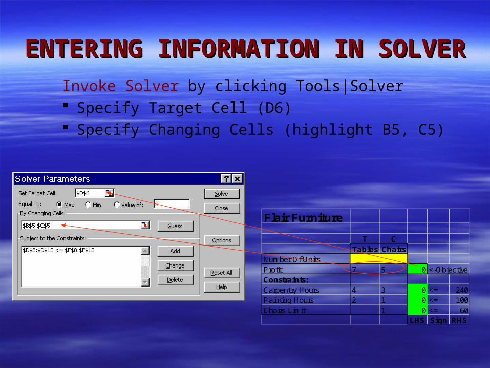
ENTERING INFORMATION IN SOLVERENTERING INFORMATION IN SOLVER

Invoke Solver by clicking Tools|Solver Specify Target Cell (D6) Specify Changing Cells (highlight B5, C5)

Flair Furniture

T CTables Chairs

Number Of UnitsProfit 7 5 0 <-ObjectiveConstraints:Carpentry Hours 4 3 0 <= 240Painting Hours 2 1 0 <= 100Chairs Limit 1 0 <= 60

LHS Sign RHS

CONSTRAINTSCONSTRAINTSSpecifying Constraints

Use "Add" constraints to enter relevant cell references for

LHS and RHS.

Either add constraints one at a time or add blocks of

constraints having same sign (<=, >=, or =) at the same

time.

Since all constraints have same <= sign one chose to

highlight all LHS D8:D10 on left and F8:F10 on right

with <= sign.

CONSTRAINTSCONSTRAINTS Specifying Constraints

SOLVER OPTIONSSOLVER OPTIONS Click on Options

button to get Solver Options window

One must check boxes titled– Assume Linear

Model – Assume Non-

Negative

SOLVING MODELSOLVING MODEL When Solve button is clicked, Solver executes model and results appear as shown.

Solver Results window also indicates the availability of three reports –

- Answer.

- Sensitivity.

- Limits.

SSOLUTIONOLUTIONOptimal solution indicated that one should make 30 Tables

and 40 chairs with an optimal profit of $ 410.

Flair Furniture

T CTables Chairs

Number Of Units 30 40Profit 7 5 410 <-ObjectiveConstraints:Carpentry Hours 4 3 240 <= 240Painting Hours 2 1 100 <= 100Chairs Limit 1 40 <= 60

LHS Sign RHS

PPOSSIBLE MESSAGES IN OSSIBLE MESSAGES IN RESULTS WINDOWRESULTS WINDOW

FFLAIR FURNITURE SOLVER ANSWER LAIR FURNITURE SOLVER ANSWER REPORTREPORT

UUSING SOLVER TO SOLVE SING SOLVER TO SOLVE HOLIDAY MEAL CHICKEN RANCH HOLIDAY MEAL CHICKEN RANCH

PROBLEMPROBLEM

LP formulation for this problem is as follows:

Minimize cost (in cents) = 2A + 3B

subject to constraints

5A + 10B 90 (protein constraint)

4A + 3B 48 (vitamin constraint)

½A 1½ (iron constraint)

A, B 0 (nonnegativity)

HOLIDAY MEAL CHICKEN RANCH HOLIDAY MEAL CHICKEN RANCH PROBLEM SPREADSHEETPROBLEM SPREADSHEET

EEXCEL LAYOUT AND SOLVER XCEL LAYOUT AND SOLVER ENTRIESENTRIES

SSOLVER ANSWER REPORTOLVER ANSWER REPORT

SUMMARYSUMMARY A mathematical modeling technique called linear

programming (LP) is introduced LP models are used to find an optimal solution to

problems that have a series of constraints binding the objective value.

How models with only two decision variables can be solved graphically is shown

To solve LP models with numerous decision variables and constraints, one need a solution procedure such as simplex algorithm.

How LP models can be set up on Excel and solved using Solver is demonstrated

LINEAR PROGRAMMING SOLUTION TECHNIQUES: GRAPHICAL AND COMPUTER METHODS.

Documents

Transcript of LINEAR PROGRAMMING SOLUTION TECHNIQUES: GRAPHICAL AND COMPUTER METHODS.