LINEAR PROGRAMMING FOR THE OPTIMAL CONTROL … · LINEAR PROGRAMMING FOR THE OPTIMAL CONTROL OF A...

LINEAR PROGRAMMING FOR THE OPTIMAL CONTROL OF AONE-DEGREE-OF-FREEDOM OVERHEAD CRANE SYSTEM

Luiz Vasco Puglia, [email protected] Universitário da FEI, Mestrado em Engenharia Mecânica, São Bernardo do Campo, São Paulo, Brazil

Fabrizio Leonardi, [email protected] Universitário da FEI, Mestrado em Engenharia Mecânica, São Bernardo do Campo, São Paulo, Brazil

Marko Ackermann, [email protected] Universitário da FEI, Mestrado em Engenharia Mecânica, São Bernardo do Campo, São Paulo, Brazil

Abstract. This work discusses the use of the Linear Programming as an alternative for solving optimal control problemsof time variant linear dynamic systems described in the discrete time state space where the elements of the control vectorare the design free variables. Since the state vector at any sampling time can be written as a linear combination of controlvector and initial state vector, a standard Linear Programming problem results. The cost function can be adapted tothe particular optimization problem to be solved. One possible goal in optimal control problems is minimizing the sumof the absolute values of the control. Another possibility is to maximize the mean speed to indirectly solve a minimumtime problem. These and other cost functions are easily formulated in the standard Linear Programming framework, i.e.,as a linear combination of the control vector. A cart-pendulum lab system was considered to illustrate this alternativeapproach. The minimum control effort has been addressed explicitly in the cost function and the minimum time problemhas been achieved indirectly by solving a series of minimum-effort problems with decreasing final time until feasibilitycould no longer be achieved. Restrictions of null angle and angular velocity at the extremes were incorporate in thedesign specification as well as other physical constraints. Results obtained illustrate that, in fact, the technique is simple,powerful and conclusive as the numerical solution of Linear Programming problems guarantees convergence to a globaloptimum provided there is a feasible solution.

Keywords: Linear Programming, Optimal Control, Time Control Low, Anti-oscillatory Control.

1. INTRODUCTION

The problem of optimal control of overhead cranes has been receiving attention from the scientific community becauseof undeniable practical relevance. Several approaches Cheng and Chen (1996), Auerning (1987), Cruz et al. (2009), Chenet al. (2007), Nassif et al. (2010), Garrido et al. (2008) and Lee (2005) have been proposed to address the problem ofminimum time and differ, for example, with respect to the model utilized, the constraints imposed and the performanceindex optimized.In load transfer operations by a crane, a major problem is optimizing the movement from origin to destination, satisfyingconstraints related to the equipment such as the kinematics of the movement. The carrier may be considered primarily asa cart-pendulum system, where the length of the pendulum is usually variable, representing the lifting.One difficulty in solving optimal control problems such as the optimal load transfer by a crane, is the necessity of solvinga two-point boundary problem with constraints on the initial and final states. For example, a linear quadratic regulatorgenerates an optimal control law but the final state can not be pre-determined. This limitation is discussed e.g. by Bem-porad et al. (2001) and Blanchini (1994).The objective function can be adapted to the particular optimization problem to be solved. A possible objective in optimalcontrol problems is minimizing the sum of the absolute control value. Another possibility is maximizing the average speedto indirectly solve the minimum time problem. These and other objective functions are easily written in the standard formof a linear programming problem, i.e., as a linear combination of the control vector.This paper discusses the use of Linear Programming as an alternative for solving this type of optimal control problem,assuming that the system dynamics are linear, time variant and expressed in the discrete time domain. In this scenario thediscrete values of the control vector are the free design variables and the state vector at any sampling time may be writtenas a linear combination of the control vector and the initial conditions. This results in the standard structure of a LinearProgramming (LP) problem.A cart-pendulum lab system was considered to illustrate the approach. The movement cycle begins and ends at givenpositions and the load is at rest in both, the beginning and end of cycle. Moreover, in the application considered here, thelifting takes place at the beginning and end of the cycle with the cart stationary, i.e., there is no lift during cart movement.A more efficient strategy is obviously to perform lifting and cart translation simultaneously, but this work intended toshow the potential of the methodology, applying it to a lab-scale system that has no motorized lifting.

ABCM Symposium Series in Mechatronics - Vol. 5 Copyright © 2012 by ABCM

Section II – Control Systems Page 222

2. METHOD

The optimal control problem of a dynamical linear system in the discrete time state space can be written in the formof a standard LP problem.

2.1 Linear Dynamics as LP Constraints

Consider the time-variant dynamic system in discrete time with a constant sampling time T and described in the statespace.

x(k+1) = A(k)x(k) +B(k)u(k) , k = 0, 1, 2... (1)

For any sampling time nT we can write

x(n) =(A(n−1).A(n−2) · · ·A(2).A(1).A(0)

)x(0)+

+(A(n−1).A(n−2) · · ·A(2).A(1)

)B(0)u(0)+

+(A(n−1).A(n−2) · · ·A(2)

)B(1)u(1) + · · ·

· · ·+(A(n−1)

)B(n−2)u(n−2)+

+ B(n−1)u(n−1)

x(n) = Fx(0) +GU

(2)

where

F = A(n)

G =[A(n−1)A(n−2) · · ·A(1)A(0)

].diag

([B(0)B(1) · · ·B(n−2)B(n−1)

])U =

[u(0)u(1) · · ·u(n−2)u(n−1)

]T (3)

where the following definitions apply

A(n) ∆= A(n−1).A(n−2) . . . A(2).A(1).A(0)

A(n−1) ∆= A(n−1).A(n−2) . . . A(2).A(1)

A(n−2) ∆= A(n−1).A(n−2) . . . A(2)

...A(2) ∆

= A(n−1).A(n−2)

A(1) ∆= A(n−1)

A(0) ∆= I

(4)

If the system is time invariant, the formulae above still hold but a standard matrix power must be used instead with thesingle system matrix A, i.e., Aj = A.A . . . A.A.Note that it is possible to represent the dynamic model in the form of constraints in the form of AX = B, which mayinclude the initial conditions x(0) and the final conditions x(n) at the nT instant

GU = x(n) − Fx(0)

AX = B (5)

where

A = GX = UB = x(n) − F x(0)

(6)

Note that the system dynamics was represented by linear constraints on the control vector. For state constraints in theform of inequalities of type x(m) ≥ η, we can write:

x(m) = F1 x(0) +G1 U1

F1 x(0) +G1 U1 ≥ ηG1U1 ≥ η − F1 x(0)

A1X1 ≥ B1

(7)

To completely define the LP problem it remains to define a cost function which is linear on states and control. The choiceof cost function depends on the optimization problem to be solved. For example, one can maximize the average speed orminimize the fuel consumption to travel a given distance.


Section II – Control Systems 23

y

mL g

g

x

f

mT

l

xT

Figure 1. Cart-pendulum scheme.

2.2 Mechanical Model

A scheme of a cart-pendulum system is shown in Fig. 1where mT = is the cart mass, mL = the load mass, xT = the cart position and ϕ = the load angle.The equations of motion describing the dynamics of the cart-pendulum model were derived using the Newton-Euler for-malism as described in Schiehlen (1997) yielding

−xT cos ϕ+ ϕl = −gsenϕ− cϕ

mL, (8)

where g is the gravity acceleration and c a damping constant.In handling anti-oscillatory problems, it is expected that, the maximum oscillation angle be small (< 10◦). This conditionleads to the approximations, senϕ ≈ ϕ and cosϕ ≈ 1. These approximations simplify the equations of motion to

−xT + ϕl = −gϕ− cϕ

mL. (9)

2.3 Optimal Control

The objective function chosen here is the control effort in the form of the sum of the absolute control values |u0| +|u1| + · · · + |un−1|. The LP admits a single objective function but we used an approach to minimize both the controleffort and the time of operation. The minimum time is obtained by solving a series of minimal-effort LP problems withdecreasing final time until contraints can no longer be satisfied. From equation (9) and defining c = c

mLand u = xT as

the control variable, we get

u = lϕ+ cϕ+ gϕ. (10)

In order to impose boundary conditions on the initial and final position and speed of the cart we create two new states x3

and x4 , which describe the position and speed of the cart yielding the following state equations

x1 = ϕ x1 = x2

x2 = ϕ x2 = u−gx1−cx2

lx3 = xT x3 = x4

x4 = xT x4 = u

(11)

With the initial condition x(t0) and final condition x(tf ), the boundary conditions are

x1(t0) = 0 x1(tf ) = 0x2(t0) = 0 x2(tf ) = 0x3(t0) = 0 x3(tf ) = 0.25mx4(t0) = 0 x4(tf ) = 0

(12)

Based on the limitations of the real plant we imposed

x4,max = 2m/sumax = 0.9m/s2

(13)

Rewriting Eq. 11x1

x2

x3

x4

=

0 1 0 0− g

l − cl 0 0

0 0 0 10 0 0 0

x1

x2

x3

x4

+

01l01

u (14)



2.4 Testing Apparatus

In order to validate the numerical results and implement the proposed control law, we used a lab equipment that allowsinverted pendulum or simple pendulum experiments. The schematic diagram of the equipment and its photo is shown inFig. 2.

Plant

Drive

Gain

P3

Feedback P4

x

x

-

+

-

Figure 2. Schematic diagram of the equipment and its photo.

The pendulum consist of a 0.215kg mass connected to the cart by a rod. The mass can be fixed on the rod at differentdistances from the cart. The cart driver has a position control system with a speed compensation. In this loop there is accessto the reference signal and the cart position and speed signals. There is also access to the pendulum angular position signal(not shown in the figure). Since the implementation details of this internal control system are not documented we choseto consider this as part of the cart sub-system and its transfer function was experimentally identified via step excitationand we selected a second order transfer function

P(s) =Knω

2n

s2 + 2ζωns+ ω2n

and found, Kn = 0.025, ωn = 31rd/s, ζ = 0.35. We also determined the gain values for the speed and cart positionsensors, Ktaco = 4V/m/s and Kpot = 40V/m, respectively

3. RESULTS

3.1 Simulation

The state equation was discretized with a sampling time T = 15ms and the optimal control vector, was obtained forN sampling periods.The rod length was set to l = 0.24m and after simple binary search, we found N = 74 as the minimum number ofsampling periods that still leads to a feasible solution. The results are presented in Fig. 3.From the results we concluded that the maximum angle os oscillation was ϕ = 10◦ and therefore the max oscillation

amplitude constraint was satisfied. The minimal response time was t = T (N) = 0.015(74) = 1.11 s.Within the Matlab environment, the SimMechanics, allows studying a nonlinear mechanical system behavior, without thenecessity of obtaining the corresponding differential equations. Figure 4 shows the model used in SimMechanics, as wellas the nonlinear (8) and linear (9) models, all within the Simulink environment. The optimal controle solution u(t) wasused as input to each of these models. The results of the integration of each of these models are presented in Fig. 5 andFig. 6 for the angle and angular velocity, respectively.

3.2 Experimental Results

The optimal control problem was formulated considering the cart acceleration as the manipulated variable. So weneed a way to impose the cart kinematics in the presence of modeling errors and disturbances. This was achieved througha state feedback control system with a feed-forward action for the acceleration as illustrated in the block diagram of Fig.7. Note that, although there is a control loop to assure cart kinematics follows the prescribed trajectories, the optimalcontrol itself is open loop, since there is no feedback for the angle trajectory. From P(s) =

x(s)

V drive(s)and imposing

V drive(t) = 1(Knω2

n)

(2ζωnx(t) + ω2

nx(t) + v(t)), where v(t) is the new manipulated variable, we form a plant model

P(s) as a double integrator, or v(t) = x(t).The control system shown in Fig. 7 has three references that are consistent with each other - position, velocity andacceleration of the cart. The position and velocity are states and, therefore, their references apply to the loop, while thedesired acceleration enters as a feed-forward action through a block that contains the inverse plant model. The gains



-1

0

1

0 0.15 0.3 0.45 0.6 0.75 0.9 1.05-0.2

-0.1

0

0.1

0.20

0.1

0.2

0

0.1

0.2

accela

ration

[m/s

ec ]2

speed

[m/s

ec]

positio

n [m

]angle

[ra

d]

time [sec]

Figure 3. Simulation with 74 sampling periods.

Nonlinearized

Theta_Dot SM

Theta SM

Theta Lin

Theta_Dot Lin

Theta Nonlin

Theta_Dot Nonlin

xT

Trilho

B F

Trigonometric Function1

sin

Trigonometric Function

cos

Sensor Theta _Dot

Sensor Theta

Sensor Carro

Revolute

B FRepeating

Sequence

Product

MachineEnvironment

Env

Linearized

1/Ls

s +K/L.s+g/L2

Joint Actuator

Integrator4

1/s

Integrator3

1/s

Integrator2

1/s

Integrator1

1/s

Integrator

1/s

Ground

Gain4

-1

Gain3

-1

Gain2

g

Gain1

-1/L

Gain

-1

Carro

CS1 CS2

Body

CS2 CS1

Add

Figure 4. Block diagram of the model.

K1 = 30992 and K2 = 1223 are the gains from state feedback and were tuned interactively in order to obtain goodtracking of the reference signals and for disturbances rejection. Because this control loop can not be perfect, the optimalcontrol problem will contain errors because the cart acceleration will never be imposed with a infinite precision. Thecontrol system of Fig. 7, along with the trajectory generation and data aquisition, were implemented in Simulink in realtime through a data acquisition board and Matlab Windows Target. Figs. 8, 9 and 10 show a comparison between thecomputers and measured position, speed and pendulum angle, respectively. Thin lines were used for generated signals



an

gle

[ra

d]

time [sec]

0-0.2

-0.15

-0.1

-0.05

0

0.05

0.1

0.15

0.2

linearizedNonlinearSimMechanics

0,15 0,30 0,45 0,60 0,75 0,90 1,05

Figure 5. Comparison of the pendulum angle among SimMechanics, linear and nonlinear equations.

time [sec]

linearizedNonlinearSimMechanicsa

ngula

rspeed [r

ad/s

]

0,15 0,30 0,45 0,60 0,75 0,90 1,05

-2

-1.5

-1

-0.5

0

0.5

1

Figure 6. Comparison of the angular speed among SimMechanics, linear and nonlinear equations

Ktaco-1

Ktaco Kpot

XX

Kit Bytronics

s + 2 s +zwn wn2 2

Kn wn2

1

s

Kpot-1

1

Kn wn2

K1

K2

wn2

2zwn

V DRIVEV

+ + +

+ ++

-

-

+

+

+

-

-

XrXrXr

s

Figure 7. Cart control system.

and thick lines for the measured signals. Since the experimental apparatus does not have an acceleration sensor for the



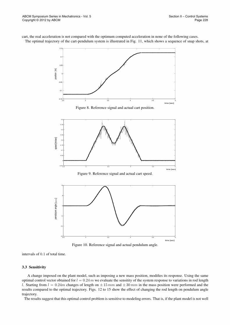
cart, the real acceleration is not compared with the optimum computed acceleration in none of the following cases.The optimal trajectory of the cart-pendulum system is illustrated in Fig. 11, which shows a sequence of snap shots, at

2.5 3 3.5 4 4.5 5-0.15

-0.1

-0.05

0

0.05

0.1

0.15

time [sec]

posi

tion

[m]

Figure 8. Reference signal and actual cart position.

time [sec]

2.5 3 3.5 4 4.5 5-0.05

0

0.05

0.1

0.15

0.2

0.25

0.3

0.35

0.4

spee

d [m

/sec

]

Figure 9. Reference signal and actual cart speed.

time [sec]

2.5 3 3.5 4 4.5 5-15

-10

-5

0

5

10

pend

ulum

ang

le [

]de

gree

s

Figure 10. Reference signal and actual pendulum angle.

intervals of 0.1 of total time.

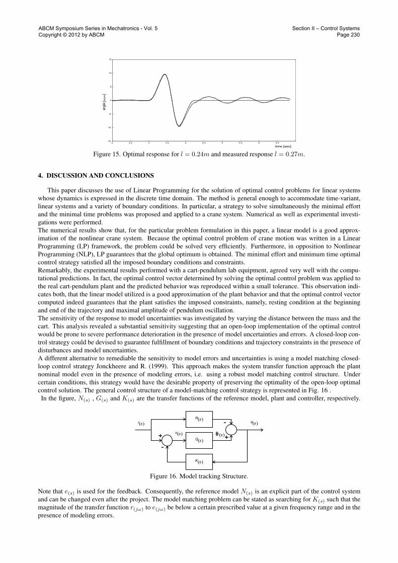
3.3 Sensitivity

A change imposed on the plant model, such as imposing a new mass position, modifies its response. Using the sameoptimal control vector obtained for l = 0.24m we evaluate the sensitity of the system response to variations in rod lengthl. Starting from l = 0.24m changes of length on ± 15mm and ± 30mm in the mass position were performed and theresults compared to the optimal trajectory. Figs. 12 to 15 show the effect of changing the rod length on pendulum angletrajectory.

The results suggest that this optimal control problem is sensitive to modeling errors. That is, if the plant model is not well



start end

Figure 11. The optimal trajectory snap shots for l = 0.24m.

2 2.5 3 3.5 4 4.5 5 5.5 6 6.5 7-15

-10

-5

0

5

10

15

angl

e [

]de

gree

s

time [sec]

Figure 12. Optimal response for l = 0.24m and measured response l = 0.21m.

angl

e [

]de

gree

s

time [sec]

2 2.5 3 3.5 4 4.5 5 5.5 6 6.5 7-15

-10

-5

0

5

10

15


angl

e [

]de

gree

s

time [sec]

2 2.5 3 3.5 4 4.5 5 5.5 6 6.5 7-15

-10

-5

0

5

10

15


known the optimal trajectory will not be assured. This sensitivity is due to the system is running with no feedback on angle.



angl

e [

]de

gree

s

time [sec]

2 2.5 3 3.5 4 4.5 5 5.5 6 6.5-15

-10

-5

0

5

10

15


4. DISCUSSION AND CONCLUSIONS

This paper discusses the use of Linear Programming for the solution of optimal control problems for linear systemswhose dynamics is expressed in the discrete time domain. The method is general enough to accommodate time-variant,linear systems and a variety of boundary conditions. In particular, a strategy to solve simultaneously the minimal effortand the minimal time problems was proposed and applied to a crane system. Numerical as well as experimental investi-gations were performed.The numerical results show that, for the particular problem formulation in this paper, a linear model is a good approx-imation of the nonlinear crane system. Because the optimal control problem of crane motion was written in a LinearProgramming (LP) framework, the problem could be solved very efficiently. Furthermore, in opposition to NonlinearProgramming (NLP), LP guarantees that the global optimum is obtained. The minimal effort and minimum time optimalcontrol strategy satisfied all the imposed boundary conditions and constraints.Remarkably, the experimental results performed with a cart-pendulum lab equipment, agreed very well with the compu-tational predictions. In fact, the optimal control vector determined by solving the optimal control problem was applied tothe real cart-pendulum plant and the predicted behavior was reproduced within a small tolerance. This observation indi-cates both, that the linear model utilized is a good approximation of the plant behavior and that the optimal control vectorcomputed indeed guarantees that the plant satisfies the imposed constraints, namely, resting condition at the beginningand end of the trajectory and maximal amplitude of pendulum oscillation.The sensitivity of the response to model uncertainties was investigated by varying the distance between the mass and thecart. This analysis revealed a substantial sensitivity suggesting that an open-loop implementation of the optimal controlwould be prone to severe performance deterioration in the presence of model uncertainties and errors. A closed-loop con-trol strategy could be devised to guarantee fulfillment of boundary conditions and trajectory constraints in the presence ofdisturbances and model uncertainties.A different alternative to remediable the sensitivity to model errors and uncertainties is using a model matching closed-loop control strategy Jonckheere and R. (1999). This approach makes the system transfer function approach the plantnominal model even in the presence of modeling errors, i.e. using a robust model matching control structure. Undercertain conditions, this strategy would have the desirable property of preserving the optimality of the open-loop optimalcontrol solution. The general control structure of a model-matching control strategy is represented in Fig. 16 .In the figure, N(s) , G(s) and K(s) are the transfer functions of the reference model, plant and controller, respectively.

( )N s

( )G s

( )K s

+

-

+

-

( )sq

( )e s

( )u s

( )r s

Figure 16. Model tracking Structure.

Note that e(s) is used for the feedback. Consequently, the reference model N(s) is an explicit part of the control systemand can be changed even after the project. The model matching problem can be stated as searching for K(s) such that themagnitude of the transfer function r(jω) to e(jω) be below a certain prescribed value at a given frequency range and in thepresence of modeling errors.



5. REFERENCES

Auerning, J.W., 1987. “Time Optimal Control of Overhead Crane with Hoisting of the Load”. International Federa-tion of Automatic Control.

Bemporad, A., Borelli, F. and Morari, M., 2001. “Model Predictive Control Based on Linear Programming”. In Proc.American Contr. Conf.,, pp. 1 – 23.

Blanchini, F., 1994. “Ultimate Boundedness Control for Uncertain Discrete-Time Systems Via Set Setinduced Lya-punov Functions”. IEEE Trans. Automatic Control, Vol. 2, No. 39, pp. 428 – 433.

Chen, S.J., Hein, B. and Wörn, H., 2007. “Swing Attenuation of Suspended Objects Transported by Robot Manipu-lator Using Acceleration Compensation”. International Conference on Intelligent Robots and Systems.

Cheng, C.C. and Chen, Y.C., 1996. “Controller Design for an Overhead Crane With Uncertainty”. Control Eng.Practice.

Cruz, J.J., Leonardi, F. and de Moraes, C.C., 2009. “Controle Anti-Balanço de tempo Minimo usando Programaçãolinear Aplicado a um Descarregador de Navios”. Congresso Brasileiro de Automação - CBA.

Garrido, S., Adberrahim, M., Giménez, A., Diez, R. and Balaguer, C., 2008. “Anti-Swinging Input Shaping Control ofan Automatic Construction Crane”. IEEE Transactions on Automation Science and Engeneering, Vol. 5, No. 3, p.549.

Jonckheere, A.E. and R., Y.G., 1999. “Propulsion Control of Crippled Aircraft by H∞ Model Matching”. IEEETransactions on Control Systems Technology, Vol. 7, No. 2, pp. 142 – 159.

Lee, H.H., 2005. “Motion planning for three-dimensional overhead cranes with high-speed load hoisting”. Interna-tional Journal of Control, Vol. 78, No. 12, pp. 875 – 886.

Nassif, L.C.J., David, D.F.B. and Gomes, A.C.D.N., 2010. “Estratégias de Controle para reduzir Oscilações emCargas Pendulares”. XVIII Congresso Brasileiro de Automática.

Schiehlen, W., 1997. “Multibody System Dynamics: Roots and Perspectives”. Kluwer Academic Publishers.

6. Responsibility notice

The author(s) is (are) the only responsible for the printed material included in this paper



LINEAR PROGRAMMING FOR THE OPTIMAL CONTROL … · LINEAR PROGRAMMING FOR THE OPTIMAL CONTROL OF A...

Documents

Transcript of LINEAR PROGRAMMING FOR THE OPTIMAL CONTROL … · LINEAR PROGRAMMING FOR THE OPTIMAL CONTROL OF A...